


Abstract
Currently, water erosion represents one of the main environmental degradation issues in tropical watersheds. Therefore, the main objective of this research was to determine the spatial distribution of erosion susceptibility by integrating multi-criteria decision-making (MCDM) and Geographic Information Systems (GIS) in the “Las Flores” Watershed, Chiapas, Mexico, which covers an area of 2519 km2. The Analytic Hierarchy Process (AHP) was implemented in combination with twelve spatial variables: watershed curve number (CNW), topographic wetness index (TWI), sediment transport index (STI), slope (SLP), soil type (STF), distance to rivers (DTR), precipitation (PCP), drainage density (DDN), terrain curvature (CUR), land use and vegetation cover (LCI), normalized difference vegetation index (NDVI), and normalized difference water index (NDWI). The model was evaluated using a Receiver Operating Characteristic (ROC) curve based on 135 erosion points identified through multitemporal image analysis. The results reveal that the variables of SLP (19.30%), PCP (16.70%), CNW (11.89%), and LCI (10.04%) had the most influence on the modeling of erosion susceptibility. In this regard, the high and very high susceptibility categories encompass a significant portion of the basin’s territory, representing 29.20% (735.41 km2), mostly concentrated in areas near the watershed, where the highest precipitation occurs, soils with shallower layers, and areas dedicated to pastures and agriculture. The model achieved very good predictive performance, with an area under the ROC curve (AUC) of 0.82. Therefore, the resulting zoning indicates that spatial modeling can reliably represent erosion susceptibility, serving as an essential technical tool for decision-makers to optimize resource distribution and develop intervention plans in high-priority areas.
1. Introduction
Environmental degradation is defined as the deterioration of the environment caused by the depletion of natural resources such as air, water, soil, and vegetation cover, which leads to the destruction of ecosystems and the extinction of wildlife [1]. This process is caused by both natural factors and anthropogenic activities, including climate, climate change, deforestation, desertification, pollution, and population growth [2]. Specifically, within this context, one of the main causes of soil degradation is erosion, which leads to the loss of the topsoil and organic matter, both of which are essential for vegetation growth and development, reducing productivity and necessitating increased use of agricultural inputs [3,4].
Moreover, water erosion is widely recognized as the main factor contributing to soil degradation [5]. Consequently, it is considered a significant threat to the sustainability and productive capacity of agriculture [6]. According to Li et al. 2024 [7], the global mean erosion rate was estimated at 5.78 t ha−1 year−1, with a slight annual increase primarily driven by the expansion of agricultural activities and changes in land use. Additionally, tropical regions exhibit high levels of potential erosion because of high rainfall amounts and intensities recorded in these areas [8].
In this context, Mexico is particularly vulnerable to water erosion due to its rugged terrain and inadequate management of forest, agricultural, and livestock areas, which promotes surface runoff and soil loss. As stated by González et al. [9], 76% of the national territory exhibits some degree of water erosion degradation. In particular, the Grijalva–Usumacinta River Basin (GUB), located in southeastern Mexico and Guatemala, is characterized by extensive natural resources, including water resources, and its high vulnerability to extreme hydrometeorological events [10], with more than 50% of its surface characterized by steep terrain that favors erosion [11]. Furthermore, a significant increase in the frequency of high-intensity rainfall events has been detected, increasing sediment transport from upland areas to lowlands through drainage networks and reservoirs [12].
Las Flores Watershed (LFW) is located in the western region of the GUB, and its runoff contributes significantly to the storage volume of the Nezahualcóyotl (Malpaso) Reservoir, which is used for hydroelectric power generation and flood control. However, the LFW faces serious deforestation problems driven primarily by land use change from forest to agricultural land for the establishment of pastures and crops [13].
Moreover, the basin is exposed to high rates of soil loss, driven by erosion processes, as a consequence of the steep terrain characteristic of mountainous areas in tropical regions [14]. Likewise, the retention of sediments in the Nezahualcóyotl reservoir, due to the impact of upstream erosion in the contributing areas, can significantly alter the fluvial dynamics of the Grijalva River system and thereby affect sediment transport downstream [15]. In the LFW, it is estimated that areas with erosion rates greater than 100 t ha−1 yr−1 constitute 29.14% of its surface, and are mainly found in the upper zones, which emphasizes the need for comprehensive watershed management plans [16].
In response to such challenges, the use of Geographic Information Systems (GIS) has allowed the development of spatial models that facilitate the assessment of susceptibility to different hydrometeorological and environmental hazards [17,18]. For this reason, the use of multiple parameters associated with relief, hydrology, climate, and current vegetation conditions is necessary, as these elements directly influence the analysis processes [19]. In this context, multi-criteria decision-making (MCDM), through robust methodologies such as the Analytic Hierarchy Process (AHP) developed by Saaty (1984) [20], emerges as a viable approach for integrating these multiple parameters. This allows the prioritization of high-risk areas and supports decision-making concerning sustainable natural resource management in watersheds [21], which are considered as the ideal territorial units for designing, establishing, and implementing intervention plans that incorporate conservation practices and runoff control measures [22,23].
The objective of this research was to determine the spatial distribution of erosion susceptibility by integrating Multi-Criteria Decision-Making and Geographic Information Systems in the Las Flores Watershed, Chiapas, Mexico. The results will contribute to a better understanding of the spatial behavior of the factors influencing erosion processes, providing a basis for identifying priority areas and developing intervention plans that incorporate conservation practices aimed at runoff control.
2. Materials and Methods
2.1. Study Area
The Las Flores Watershed (LFW) is located in the western part of the state of Chiapas, Mexico, within Hydrological Region 30 (Grijalva-Usumacinta) from 16°18′02.79″ to 16°47′34.98″ North latitude and 94°10′06.94″ to 93°24′13.90″ West longitude. Its catchment area covers 2519.03 km2, and its main stream is the La Venta River, which is 103.35 km long. The river originates from the confluence of the Zoyatenco and Cintalapa Rivers in the upper part of the mountainous Sierra Madre de Chiapas and extends to its outlet point (16°41′41.70″ N, 93°33′38.29″ W) at the Las Flores Hydrometric Station (LFHS) (Figure 1).
Figure 1.
Location of the Las Flores Watershed (LFW), Chiapas, Mexico.
According to the Köppen climate classification modified by García [24], the predominant climate is warm subhumid (Aw) with summer rains, with an annual precipitation average of 953.94 mm and a mean monthly temperature of 24 °C [25]. Regarding topography, the elevation within the LFW varies from 485 to 1946 m, with a mean altitude of 748.41 m and a mean slope of 10.17%, placing the watershed in a moderately rugged and rolling relief with pronounced local variations that influence surface runoff velocities [26].
2.2. Analytic Hierarchy Process with Geographic Information Systems
The Analytic Hierarchy Process (AHP) is a multi-criteria decision-making (MCDM) technique used to analyze complex problems and is commonly employed, in combination with Geographic Information Systems (GIS), for the spatial modeling of soil erosion risk [27,28], landslides [29,30], floods [31,32] and wildfires [33,34].
Figure 2 presents the workflow for assessing erosion susceptibility in the LFW using the AHP-GIS methodology.
Figure 2.
General AHP-GIS workflow methodology.
The AHP-GIS methodology is primarily based on assigning weights to different parameters derived from geospatial information, which directly influence the analysis process and provide technical support for decision-makers in the integrated management of natural resources [18].
In general, the procedure for determining the weights of each parameter consists of three stages: (1) construction of the pairwise comparison matrix, (2) determination of the relative weights of each criterion, and (3) verification of matrix consistency [20].
The parameters considered are described below: Curve Number (CNW), Topographic Wetness Index (TWI), Sediment Transport Index (STI), Slope (SLP), Soil Type (STF), Distance to Rivers (DTR), Precipitation (PCP), Drainage Density (DDN), Curvature (CUR), Land Use and Vegetation Cover (LCI), Normalized Difference Vegetation Index (NDVI), and Normalized Difference Water Index (NDWI). In addition, Table 1 presents the data type, description, spatial resolution and/or scale, and data source used to generate each parameter.
Table 1.
Geospatial variables used to assess water erosion susceptibility in the Las Flores Watershed.
2.2.1. Pairwise Comparison Matrix
The pairwise comparison matrix (D) was constructed based on the number of parameters influencing erosion processes (n) using Equation 1, considering the specific importance level of one parameter relative to another based on the scale of relative significance developed by Saaty [20], which contains different importance ranges from 1 to 9 according to Table 2.
where i and j = 1, 2, …, n corresponds to the number of the evaluation parameter.
Table 2.
Saaty comparison scale [20].
2.2.2. Determination of the Relative Weights of Each Criterion
Subsequently, the normalized decision matrix (R) was constructed by dividing each element (aij) of matrix D by the sum of its corresponding column (Sj) using Equation (2), aimed at standardizing the scales and ensuring comparability among the different evaluation parameters.
Afterwards, the parameter weight vector (W) is calculated, where each value (wj) corresponds to the average of the normalized elements of each row (rij) of matrix R using Equation (3).
where rij is the element of the normalized matrix for the i-th row and the j-th parameter, and wj corresponds to the relative weight of each parameter influencing the evaluation of erosion processes.
The vector W corresponds to the relative weighting of each criterion within the AHP method and represents the primary input for conducting the multicriteria evaluation.
2.2.3. Verification of Matrix Consistency
Finally, the consistency of matrix D is verified, as it may be influenced by the evaluators’ knowledge, which in some cases can introduce inconsistencies and affect the coherence of the parameters used in the assessment.
Therefore, evaluating its consistency is recommended to ensure the proper application of the relative weights assigned to each parameter. The consistency vector (CV) is obtained from the matrix product of matrix D and the weight vector W, whose elements are divided by the corresponding relative weight (wj) using Equation (4).
where cvi, corresponds to the consistency vector of each parameter.
Subsequently, the maximum eigenvalue (λmax) is determined from the average of the components of the consistency vector CV (Equation (5)). Based on this result, the consistency index (CI) is calculated (Equation (6)), where cvi corresponds to the consistency vector for each parameter.
Lastly, the consistency ratio (CR) is evaluated from the relationship between the consistency index (CI) and the random consistency index (RI), whose values were defined by Saaty [20] as a function of the number of parameters (n) of matrix D (Table 3).
Table 3.
Values of average random consistency index RI.
If the CR value is less than or equal to 0.10, matrix D is considered consistent, and therefore, acceptable; otherwise, the pairwise comparison of matrix D must be performed again until an acceptable CR value is obtained.
2.3. Thematic Layers
In the application of the AHP-GIS methodology, it is essential to consider a range of variables grouped into distinct thematic categories that directly influence sediment transport dynamics [39].
Figure 3 shows the spatial variables used, including hydrological parameters that directly affect the capacity for surface runoff generation, such as the watershed curve number (CNW), sediment transport index (STI), distance to rivers (DTR), and drainage density (DDN); topographic variables that condition flow velocity, acceleration, and direction, such as the topographic wetness index (TWI), slope (SLP), and terrain curvature (CUR); as well as edaphic factors that determine the natural soil resistance (STF) and climatic factors representing the direct erosive force of rainfall (precipitation, PCP). Furthermore, multispectral satellite image indices are incorporated to reflect the surface protection provided by vegetation cover, such as land use and vegetation cover (LCI), normalized difference vegetation index (NDVI), and normalized difference water index (NDWI).
Figure 3.
Thematic layers of the Las Flores Watershed (LFW): (a) watershed curve number (CNW); (b) topographic wetness index (TWI), (c) sediment transport index (STI), (d) slope (SLP); (e) soil type (STF); (f) distance to rivers (DTR); (g) precipitation (PCP); (h) drainage density (DDN); (i) terrain curvature (CUR); (j) land use and vegetation cover (LCI); (k) normalized difference vegetation index (NDVI); (l) normalized difference water index (NDWI).
2.3.1. Watershed Curve Number (CNW)
The CNW represents the capacity of a soil to facilitate water infiltration based on land use and land cover, as well as the energy and surface runoff generation potential according to the hydrological characteristics of the land surface, where higher values indicate a greater runoff potential and, therefore, a higher risk of erosion [40]. According to Hernández-Jiménez [41], the determination of the curve number (CN) is performed in two stages. First, the hydrologic soil group is identified based on the soil unit that describes the STF and its main characteristics. Second, the CN value is assigned according to the land use and hydrological condition. Furthermore, according to the Natural Resources Conservation Service (SCS), runoff potential and infiltration rates are determined based on the hydrologic soil group [42]. The first group (Group A) consists of soils with the lowest runoff potential and the highest infiltration rate and is composed of deep sands and gravels that drain rapidly. The second group (Group B) corresponds to soils with a moderately low runoff potential and moderate infiltration rates, generally consisting of loamy or sandy loam soils. The third group (Group C) contains soils with moderately high runoff potential and slow infiltration rates, often due to restrictive layers or moderately fine textures such as clay loam soils. Finally, the fourth group (Group D) comprises soils with the highest runoff potential and the lowest infiltration rate, encompassing clay soils with high swelling potential, high water tables, or nearly impermeable layers.
In Mexico, INEGI uses the soil classification system of the Food and Agriculture Organization (FAO) World Reference Base for Soil Resources [43] to represent the spatial distribution of soil types [35]. Table A1 in Appendix A presents the classification of hydrologic soil groups in the LFW based on soil unit and texture.
Likewise, CN values were assigned according to Table A2 in Appendix A, based on land use, hydrological condition, and soil group in the LFW, using INEGI’s spatial land use distribution map [36] (Figure 3a).
2.3.2. Topographic Wetness Index (TWI)
The TWI permits the identification of areas with greater water retention in the terrain, conditions that favor a reduction in the cohesion of the soil surface layer [21]. Likewise, high TWI values indicate a greater propensity for moisture accumulation and water saturation, which directly translates into an increased risk of erosion and landslides [28]. The TWI was determined from the spatial distribution of elevation in the LFW [26] using Equation (8) [44], with the WhiteboxTools plugin from the software QGIS (Figure 3b).
where α is the specific drainage area per unit contour width (m2 m−1) and β is the slope of the terrain (radians).
2.3.3. Sediment Transport Index (STI)
The STI represents the spatial distribution of the potential for particle detachment, movement, and redistribution by surface runoff across the terrain [45]. A high value shows conditions under which the force of water can erode and transport large volumes of sediment, accelerating the formation of rills, landslides, and surface degradation [28]. This variable is important for understanding the magnitude and extension of the erosion process in different areas. The STI was calculated from the spatial distribution of elevation [26] using Equation (9) [46], with QGIS software (3.40.14-Bratislava) with the WhiteboxTools plugin (Whitebox Workflows for QGIS, Version 2.1.3) (Figure 3c).
where α is the specific drainage area per unit contour width and β is the slope of the terrain (radians). 22.13 and 0.0896 values correspond to the standard length and slope factors of the unit plot in the Universal Soil Loss Equation (USLE).
2.3.4. Slope Gradient (SLP)
The SLP is one of the factors with the greatest influence on erosion, as areas with higher values increase surface runoff velocity, consequently reducing infiltration capacity and favoring soil particle detachment [45]. The importance of this variable lies in its ability to determine areas at higher risk of erosion processes, allowing the identification of areas where the implementation of conservation measures is appropriate [21]. Slope (SLP) was calculated as a percentage from the spatial distribution of elevation in the LFW [26] using the raster analysis tools in ArcMap software (10.8) (Figure 3d).
2.3.5. Soil Type (STF)
The STF defines susceptibility to erosion processes, as its characteristics control the amount of water that infiltrates into the system and directly influence percolation and permeability, thereby promoting moisture conservation in the watershed [47]. This variable was obtained from the spatial distribution of soil types provided by INEGI [35] (Figure 3e).
2.3.6. Distance to Rivers (DTR)
DTR allows the identification of areas where the action of surface runoff compromises terrain stability, as areas near stream margins are exposed to various erosive mechanisms, such as sediment detachment by currents and lateral erosion along slopes [48]. This variable was calculated using the Euclidean Distance tool in ArcMap, applied to the entire LFW catchment area and using its drainage network as the reference [37], thereby generating a continuous proximity layer representing the linear distance to stream channels (Figure 3f).
2.3.7. Precipitation (PCP)
PCP is considered one of the main agents of water erosion and sediment transport, as the magnitude of soil loss is directly proportional to the kinetic energy and intensity of rainfall [49]. For its integration into the analysis, the spatial distribution of precipitation across the INEGI climatic units was used [25] (Figure 3g).
2.3.8. Drainage Density (DDN)
The DDN is an important indicator of the hydrological potential of a watershed, as it permits the characterization of aspects such as erosion, permeability, slope, and vegetation cover [50]. According to Ahmed et al. [51], high DDN values are associated with a greater capacity for sediment transport by surface runoff and, as a result, an increased risk of erosion. This variable was calculated using the Line Density tool in ArcGIS v10.8 and the drainage network provided by INEGI [37] (Figure 3h).
2.3.9. Terrain Curvature (CUR)
The CUR represents the shape of the land surface based on the second derivative of elevation, and is classified as convex, concave, or flat [52]. This relief characteristic influences soil formation processes and surface water movement, as areas with concave curvature tend to converge and concentrate runoff, promoting moisture accumulation and particle detachment; in contrast, convex areas disperse the flow [53]. In addition, profile curvature has been shown to be a significant variable for predicting gully erosion [54]. This variable was calculated from the spatial distribution of elevation in the LFW [26] using the raster analysis tools in ArcMap software (Figure 3i).
2.3.10. Land Use and Vegetation Cover (LCI)
The LCI represents the land activity category occurring in a given area, such as agriculture, human settlements, forests, tropical forests, or grasslands. Agricultural activities can increase soil erosion susceptibility when vegetation cover is insufficient to protect the soil surface, leaving soil particles more exposed to detachment and transport by runoff [55]. For this variable, the spatial land cover distribution map from INEGI [36] was used (Figure 3j).
2.3.11. Normalized Difference Vegetation Index (NDVI)
The NDVI represents the current state of vegetation in a given area using multispectral satellite imagery bands [56]. According to Bagwan et al. [57], this index is an crucial parameter for evaluating erosion susceptibility, as vegetation cover density is considered the most important factor influencing surface runoff in a watershed [58].
This index ranges from −1 to 1, where higher values correspond to healthy and dense vegetation, whereas lower or negative values are associated with bare soil, water, or stressed vegetation [28]. For its calculation, a total of 172 Sentinel-2 satellite images were processed via a script in the Google Earth Engine platform for the 2021–2025 period at a spatial resolution of 10 m [38].
A cloud cover threshold of less than 10% was applied to exclude high-cloud scenes. NDVI was calculated for each image using Equation (10), and the pixel-wise median of the resulting time series was taken as the final layer (Figure 3k).
where ρNIR and ρRED are the surface reflectance values of the near-infrared and red bands, respectively.
2.3.12. Normalized Difference Water Index (NDWI)
The NDWI, as proposed by McFeeters [59], is based on the contrast between green and near-infrared reflectance and highlights surface water content. Higher values are associated with water bodies, saturated surfaces, and sparse or stressed vegetation, whereas lower values correspond to dense, healthy vegetation.
In this study, high NDWI values were interpreted as greater surface moisture and reduced vegetation protection, which may increase soil susceptibility to water erosion, especially under intense precipitation conditions. Hence, this variable is relevant for identifying areas where water saturation promotes erosion and for planning management actions to minimize these risks.
For its calculation, the same Sentinel-2 surface reflectance image collection described in Section 2.3.11 (172 images, 2021–2025, 10 m, cloud cover < 10%) was used [38]. NDWI was calculated for each image using Equation (11), and the median of the resulting time series was taken as the final layer (Figure 3l).
where ρGREEN and ρNIR are the surface reflectance values of the green and near-infrared bands, respectively.
2.4. Generation and Evaluation of the Erosion Susceptibility Map
Erosion-susceptible areas are generally classified into five priority levels: very high, high, moderate, low, and very low [21,60]. Therefore, in this study, each thematic layer was reclassified on a numerical scale from 1 to 5, where lower values represent lower susceptibility and higher values indicate higher susceptibility to erosion processes. Subsequently, based on these reclassifications, the weights obtained through the AHP method were applied to each parameter to generate the final erosion susceptibility map displaying the above-mentioned categories.
Afterward, the final map was evaluated using the Receiver Operating Characteristic (ROC) curve, a widely used technique for assessing model performance [61]. The ROC curve is a plot in which the true positive rate (TPR) values, displayed on the y-axis, are plotted against the false positive rate (FPR) values, displayed on the x-axis [62].
The ROC analysis requires a binary reference; therefore, the high and very high susceptibility classes were defined as presence, since these are the categories for which intervention is prioritized [21] and which spatially coincide with the areas of highest erosion rates previously reported for the LFW [16]. The moderate class was grouped with the lower classes because it represents a transitional condition that requires land-use management rather than immediate intervention; this grouping does not imply that erosion is absent in these areas.
Based on the geometry of the ROC curve, the Area Under the Curve (AUC) is calculated, with its value representing the accuracy of the model relative to the reference data. This enables models to be classified as excellent (AUC = 0.9–1.0), very good (AUC = 0.8–0.9), good (AUC = 0.7–0.8), bad (AUC = 0.6–0.7), or unsuccessful (AUC = 0.5–0.6) [63]. That is, values close to 1 indicate high reliability, whereas values below 0.5 indicate that the model lacks predictive capacity for the phenomenon under analysis [64,65].
For this purpose, erosion areas were identified based on the location of 135 points obtained through a multitemporal analysis of high-resolution imagery in Google Earth and confirmed via field surveys across the LFW. This approach enabled the detection of erosion processes such as gullies, landslides, sediment deposits, and changes in vegetation cover, thereby providing an accurate validation.
3. Results and Discussion
3.1. Weighting of Erosion Factors Using AHP
The construction of the pairwise comparison matrix and the assignment of criteria weights were conducted through a collaborative expert judgment process involving the co-authors and specialized researchers from Instituto Nacional de Investigaciones Forestales, Agrícolas y Pecuarias, Universidad Autónoma Chapingo, and Colegio de Postgraduados (COLPOS). The panel comprised experts with over 15 years of professional experience and research specialization in environmental economics, hydrological modeling, watershed management, soil and water conservation, and geographic information systems (GIS). The level of importance for each parameter in the erosion risk model was determined through the AHP using pairwise comparisons [20]. Table 4 presents the comparison matrix among the variables: CNW, TWI, STI, SLP, STF, DTR, PCP, DDN, CUR, LCI, NDVI, and NDWI. Likewise, to verify the reliability of the results, the consistency of the pairwise comparison matrix was evaluated. The maximum eigenvalue (λmax) was 13.26 for twelve parameters, resulting in a consistency index (CI) of 0.11. Using the random consistency index (RI) of 1.48 (Table 3), the consistency ratio (CR) was 0.08. Since the CR is below the 0.10 threshold proposed by Saaty [20], the pairwise comparison matrix is considered acceptably consistent.
Table 4.
Pairwise comparison matrix of the parameters used in the LFW erosion model.
The CR value is comparable to those reported in other erosion susceptibility studies based on AHP-GIS, supporting the methodological rigor of the expert judgment applied in the pairwise comparison matrix for the LFW. Chwikhi et al. [66], in the arid region of Gabes (Tunisia), obtained a CR value of 0.059 when evaluating ten geoenvironmental criteria, whereas Mushtaq et al. [67], in the central Kashmir (Northwestern Himalayas), reported a CR = 0.07 for eleven conditioning factors. These studies, conducted under different geographic, climatic, and topographic conditions, ranging from arid areas to tropical mountain watersheds, confirm that the AHP method can provide robust and reproducible weights for modeling erosion susceptibility, regardless of the application context.
Figure 4 shows that SLP is the most relevant criterion, with an importance of 19.30%, followed by PCP at 16.70%, CNW at 11.89%, LCI at 10.04%, DDN at 8.98%, STF at 7.63%, CUR at 6.76%, STI at 5.90%, TWI at 4.63%, NDVI at 3.34%, NDWI at 3.33%, and finally DTR at 1.50%. These results are consistent with those reported by Fallah et al. [68], who indicate that topography is the determining factor in defining areas with greater vulnerability to erosion processes. This is corroborated by grouping the topographic parameters (TWI, STI, SLP, and CUR), which together account for 36.60% of the total weighting.
Figure 4.
Weights of the criteria used in the LFW erosion model.
Specifically, the individual weight of slope in the LFW is consistent with values reported in AHP-GIS studies conducted across distinct geographical and climatic contexts: Dutta et al. [69] identified slope as the factor with the highest relative weight (26.4%) when evaluating eleven geoenvironmental criteria in the Sali River basin, India, followed by soil texture (19.2%) and precipitation (13.5%); Kucuker and Cedano [70] similarly reported slope as the dominant criterion (21%) in the Oltu forestry unit, Turkey, followed by rock type (19%) and land cover (17%); whereas Olii et al. [71], using a grid-based analysis approach in the Bone basin, Indonesia, again obtained slope as the most influential factor (20.2%), followed by the sediment transport index (19.0%) and flow length to the nearest channel (12.6%). The recurrence of this pattern, regardless of the number or type of additional criteria considered, reinforces the finding that slope frequently emerges as a dominant factor across diverse contexts, given its direct control over surface runoff velocity and soil infiltration capacity.
In comparison, parameters related to vegetation cover, CNW, LCI, NDVI, and NDWI, collectively constitute 28.59% of the importance in the model. Within this group, CNW and LCI are intrinsically related and combined represent 21.92% of the total weighting, highlighting their fundamental role in surface runoff generation, consistent with the findings reported by Sanchez et al. [28], who identified the curve number as one of the most influential parameters for determining erosion zones using AHP-GIS.
Likewise, although precipitation (PCP) is considered by Mihi et al. [72] as the primary factor, in this study it ranks second in importance, underlining its important weight. In comparison, parameters related to the drainage network (DDN and DTR) comprise 10.48% of the total weighting, consistent with the results reported by França et al. [21], who reported a similar order of importance for the drainage network. Finally, STF, representing 7.63%, plays a fundamental role by governing infiltration capacity and the intrinsic resistance of soil particles to water detachment and transport, key factors determining the hydrological response of the watershed [66].
Finally, Equation (12) integrates the erosion risk index (ER) for the LFW through the spatial integration of the analyzed parameters, weighted according to their level of importance derived from the AHP.
3.2. Reclassification and Spatial Analysis of Erosion Parameters
The range and surface area corresponding to each category (very low, low, moderate, high, and very high) of the thematic layers are presented in Table 5. For integration into the multi-criteria evaluation model, each conditioning factor was standardized and spatially reclassified. With the exception of the categorical LCI and STF layers, which were reclassified based on their inherent soil erosion susceptibility and cover vulnerability levels, continuous parameters were grouped into five standardized classes using the natural breaks (Jenks) method, thereby accurately reflecting the spatial heterogeneity and surface distribution of the watershed [57]. For the spectral and topographic indices (TWI, STI, NDVI, and NDWI), the class breaks were derived from the statistical distribution of the pixel values of each layer, which minimizes the variance within classes and maximizes the differences between them; the resulting classes were then ranked from 1 to 5 according to the expected relationship between the index value and erosion susceptibility.
Table 5.
Range and area of each class of the parameters used in the erosion model.
The CNW is predominantly concentrated within the moderate class, which accounts for 55.56% of the watershed, followed by the low class at 27.15% and the high class at 10.72%, while the very low and very high classes represent 4.28% and 2.29%, respectively. This spatial distribution reflects the land cover composition of the LFW: forests and woodlands (48.07%; 1210.79 km2) exhibit good or fair hydrologic conditions due to their dense vegetation cover, whereas grasslands, the predominant land use and cover (40.45%; 1018.99 km2), were classified under fair hydrologic conditions because they are primarily located in areas with moderate slopes. These conditions explain the predominance of CNW values within the moderate range. For its part, the TWI is dominated by the very high and high classes, encompassing 41.26% and 38.77% of the watershed, respectively, whereas the moderate, low, and very low categories account for 11.88%, 6.02%, and 2.06% respectively. Conversely, the STI is dominated by the very low (55.47%) and low (30.78%) classes, followed by the moderate class at 12.03%, the high class at 1.57%, and the very high class at 0.14%. Regarding SLP, the very low class predominates with 47.35% of the area, followed by the low class with 27.65%, while the moderate, high, and very high classes account for 16.08%, 7.67%, and 1.24%, respectively. With respect to STF, the very high class covers 49.35% of the area, followed by the high class at 22.40% and the moderate class at 20.57%, whereas the low and very low classes represent 7.46% and 0.22%, respectively.
For distance to rivers DTR, the very high class accounts for 36.12% of the area, followed by the high class with 30.60%, the moderate class with 19.95%, the low class with 10.40%, and the very low class with 2.93%. Precipitation (PCP) exhibits a relatively balanced distribution between the very low (28.21%) and low (28.09%) classes, while the moderate class encompasses 24.97% of the area, followed by the high class at 17.00% and the very high class at 1.74%. Drainage density (DDN) is concentrated primarily in the moderate class (35.83%), followed by the low class (28.64%), whereas the high, very low, and very high classes account for 19.57%, 10.25%, and 5.71%, respectively. For terrain curvature (CUR), the moderate class predominates with 39.88% of the area, followed by the low class with 30.68% and the high class with 19.41%, while the very low and very high classes represent 8.36% and 1.66%, respectively.
Finally, land use and vegetation cover (LCI) is predominantly distributed within the high class, which accounts for 40.45% of the area, followed by the low class at 27.56% and the very low class at 22.65%, whereas the moderate and very high classes represent 7.25% and 2.09%, respectively. The normalized difference vegetation index (NDVI) exhibits a relatively homogeneous distribution across the high (25.32%), moderate (23.34%), and low (19.83%) classes, while the very high and very low classes cover 16.81% and 14.70% of the area, respectively. Finally, the normalized difference water index (NDWI) is predominantly represented by the moderate class at 32.96%, followed by the low at 25.36% and high at 24.68% classes, whereas the very low and very high classes account for 13.90% and 3.10%, respectively.
The spatial distribution of the analyzed parameters indicates that erosion susceptibility is governed by the interaction among topographic conditions, land use, soil type, and factors associated with the drainage network [57]. In particular, areas classified within the very high and high categories for the topographic wetness index (TWI), distance to the drainage network (DTR), and STF suggest substantial concentration of surface runoff and limited water retention and infiltration capacity, particularly in sectors located near stream channels [73]. Moreover, this condition is further increased by the presence of areas with sparse vegetation cover, including grasslands, bare soil, and urban areas, represented by the high and very high classes of LCI and NDVI, which together account for 42.54% and 42.13% of the LFW area, respectively. In the case of NDVI, the high and very high classes correspond to low index values associated with lower vegetation density or vigor. According to Rodríguez-Rastrero et al. [74], these variables are closely interrelated and can be used to assess soil degradation, highlighting how the lack of vegetation cover accelerates soil degradation and water erosion processes, mainly in agricultural areas.
The results indicate that erosion susceptibility is not determined by a single factor but rather by the spatial interaction of topographic, edaphic, hydrological, and land cover conditions. Although low and very low slopes predominate, along with low STI values and reduced precipitation levels, the presence of highly vulnerable soils, areas with sparse vegetation cover, sectors located near the drainage network, and zones with greater potential moisture accumulation may promote runoff concentration and soil loss. Therefore, areas with the highest susceptibility do not necessarily coincide exclusively with zones characterized by steeper slopes or higher precipitation, but rather with areas where multiple conditioning factors overlap, highlighting the multicausal nature of the erosion process in the LFW.
Reclassification using the Jenks natural breaks method enabled the identification of distinct spatial patterns among susceptibility classes; however, these results represent a relative estimate that depends on the quality of the input data and the weighting criteria applied in the AHP. Consequently, it is essential to compare the resulting map with empirical evidence to confirm its actual predictive capacity, as described in the statistical evaluation presented below.
3.3. Erosion Susceptibility Map
The final erosion risk (ER) map, derived from the multicriteria integration using AHP-GIS based on the factors influencing the erosion process in the LFW, illustrates the spatial distribution and potential intensity of soil degradation processes (Figure 5).
Figure 5.
Spatial distribution of soil erosion susceptibility across the LFW and location of the 135 erosion points used for validation.
On the other hand, the spatial distribution of the erosion risk categories indicates marked heterogeneity across the LFW and is distributed as follows. First, the very low class covers an area of 323.02 km2, representing 12.82% of the watershed, while second, the low class encompasses 686.44 km2, equivalent to 27.25% of the total area; both classes occur predominantly in the lower part of the watershed. Third, the moderate category represents the largest spatial extent, covering 774.16 km2, or 30.73% of the study area, and is broadly distributed throughout the territory. Fourth, the high class extends over 534.15 km2, accounting for 21.20% of the watershed, and is located primarily in the middle section. Finally, the very high class covers 201.26 km2, representing the remaining 8.00% of the total area, and occurs mainly in the headwaters of the watershed.
Overall, the moderate, low, and very low susceptibility classes dominate most of the watershed territory, collectively accounting for more than 70.80% of the total area. Nevertheless, the high and very high susceptibility categories together encompass a substantial portion of the watershed, representing 29.20% of the total area, and are located primarily in areas characterized by steeper slopes, lower vegetation-cover density, as well as grasslands and agricultural areas, that is, zones with greater vulnerability to erosion. This pattern is consistent with findings reported in various watershed studies, in which alterations to natural vegetation cover increase soil loss rates and promote sediment generation and transport toward the main stream channels [28,47,75]. Therefore, the results obtained through the integration of AHP and GIS constitute a valuable decision-support tool, enabling the prioritization of intervention areas and the implementation of soil conservation practices and runoff-control structures in the LFW. This spatial distribution agrees with previous estimates of current erosion in the LFW, where the highest erosion rates (>100 t ha−1 yr−1) were also concentrated in the upper zones and covered 29.14% of the surface area [16]. However, this similarity in extent (close to the 29.20% of high and very high susceptibility obtained in this study) should be interpreted with caution, since the previous study quantified soil loss rates, whereas the present model expresses relative susceptibility to erosion.
For the local-scale analysis, the spatial information was grouped into eight 45° sectors centered on the cardinal and intercardinal directions: north (N), northeast (NE), east (E), southeast (SE), south (S), southwest (SW), west (W) and northwest (NW), drawn from the watershed centroid. At the local scale, the high and very high susceptibility areas are concentrated in the western (W) and southwestern (SW) sectors of the watershed. Together, these sectors contain 121.92 km2 of the very high class (60.58% of the class; 4.84% of the watershed) and 244.90 km2 of the high class (45.85% of the class; 9.72% of the watershed). They include the highest terrain of the watershed, with mean elevations of 848.73 m (W) and 842.76 m (SW), maximum elevations of 1946 and 1603 m, mean slopes of 19.09 and 21.35%, and the highest mean annual precipitation (1090.79 and 1040.34 mm), respectively. Grasslands (PAST) are the largest land-cover class in these sectors (251.09 km2; 31.35%), and rainfed (AGRL) and irrigated agriculture (IRRA) add 85.51 km2 (10.67%). Shallow soils, such as Leptosols (LP) and Regosols (RG), are widespread, particularly in the western sector. The combination of higher elevation, greater rainfall, shallow soils with low water-retention capacity, and areas of pasture and agriculture limits infiltration and favors runoff concentration and sediment delivery to the main channel. In contrast, the very low and low susceptibility classes form a compact block in the northeastern (NE) and eastern (E) sectors, around the middle and lower reaches of the main channel up to the outlet. These sectors hold 164.51 km2 of the very low class (50.93% of the class; 6.53% of the watershed) and 276.64 km2 of the low class (40.30% of the class; 10.98% of the watershed). They are characterized by lower elevations (mean 639.79 m in NE and 708.51 m in E), mean slopes of 16.14 and 18.59%, and lower mean annual precipitation (840.47 and 895.22 mm), respectively. Forests cover 52.47% of these sectors (410.38 km2), mainly tropical dry forest (FRSD; 171.97 km2) and mixed forest (MIXF; 118.82 km2), while grasslands (PAST) occupy 40.65%. The lower relief and rainfall, together with the extensive forest cover, explain the lower susceptibility even in the proximity of the main channel.
These local patterns indicate that the areas of highest susceptibility are the result of multiple factors rather than any single one [57,76]. Although the western and southwestern sectors combine the highest elevations and precipitation, mean slope alone barely differentiates them from the northeastern and eastern sectors. The highest susceptibility is observed where several conditioning factors overlap: higher precipitation, shallow soils, and areas of pasture and agriculture. Accordingly, intervention should prioritize the western and southwestern sectors in the headwaters (conservation practices on slopes and runoff-control structures) and the southern and southeastern sectors in the middle section (riparian reforestation, conservation practices in productive areas, and silvopastoral systems in grassland) [77,78]. Therefore, prioritizing the sectors where several conditioning factors converge, rather than relying on slope or precipitation alone, allows conservation efforts to be directed to the areas with the greatest erosion susceptibility [79].
3.4. Validation of the Erosion Susceptibility Model
The performance of the erosion susceptibility model was evaluated using Receiver Operating Characteristic (ROC) curve analysis and calculation of the Area Under the Curve (AUC). For this validation process, the very low, low, and moderate susceptibility classes were grouped as the absence of severe erosion, whereas the high and very high categories were classified as the presence of erosion. A total of 135 erosion points were used as input data representing positive observations.
In similar AHP-GIS validations, mapped events tend to concentrate in the highest susceptibility classes [60]. However, because erosion points may also occur in the moderate susceptibility class, the distribution of the 135 points across susceptibility classes is presented in Table 6. The high and very high susceptibility classes accounted for 104 points (77.04%) across 29.20% of the area, whereas the moderate susceptibility class contained 18 points (13.33%) across 30.73% of the area, with a frequency ratio of 0.43, below unity. This indicates that, although erosional processes may occur in the moderate susceptibility class, their incidence is lower than expected given the extent of this class, supporting its classification below the prioritization threshold.
Table 6.
Distribution of the 135 erosion points across the erosion susceptibility classes and frequency ratio (FR) in the LFW.
The validation is shown in Figure 6, where the Receiver Operating Characteristic (ROC) curve yields an Area Under the Curve (AUC) value of 0.82.
Figure 6.
Area under the curve (AUC) for the validation of the LFW erosion model.
Consequently, based on the evaluation criteria proposed by Domazetović et al. [63], this score denotes very good predictive performance, reflecting a robust capacity to spatially discriminate between stable terrains and zones exhibiting high vulnerability to land degradation. This result confirms that the weights assigned to the topographic, land-use, climatic, drainage-network, and edaphic parameters accurately reflect the spatial dynamics of water-driven erosion, thus demonstrating the methodological validity of the erosion risk map generated for the LFW.
This result is consistent with the values reported in similar studies that have integrated AHP and GIS to assess water erosion susceptibility in watersheds with mountainous topography. Kucuker and Cedano Giraldo [70] obtained an AUC of 0.81 when evaluating seven erosion factors in the Oltu forest management unit, Turkey, whereas Dutta et al. [69] reported a value of 0.84 after integrating eleven geoenvironmental criteria in the Sali River basin, India. In contrast, Olii et al. [71] obtained an AUC of 0.75 in the Bone watershed, Indonesia. The AUC value obtained for the LFW falls within this range, confirming the robustness of the AHP-GIS approach for spatially representing water erosion processes, even when the number and type of criteria vary among studies [21,57,67]. Nevertheless, although the model shows very good spatial agreement, the establishment of field monitoring areas is recommended to continuously validate soil loss rates and refine the susceptibility ranges in the upper part of the LFW [80].
3.5. Analysis and Interpretation of Erosion-Susceptible Areas
Subsequently, based on the results and according to França et al. [21], the five priority levels should be addressed to reduce erosion susceptibility, considering the following categories:
- Very low: It corresponds to stable areas that are highly resistant to environmental stress and highly resilient. Therefore, the recommendations for these areas focus solely on the proper use of land according to its intended human use, the conservation of remaining vegetation in jungle and forest areas, and finally, the protection of zones with a high capacity for rapid recovery.
- Low: It shows a slight susceptibility to environmental stress while maintaining stable and resilient conditions. Therefore, the recommended actions include the use of land compatible with the productive capacity of the terrain, the application of conventional recovery techniques under proper management, and likewise, the conservation of the vegetation cover of jungles and forests.
- Moderate: They are areas characterized by a moderate level of risk to susceptibility to erosion processes, and correspond to transition zones between stable and unstable conditions. Therefore, these areas require strict land use management, prioritizing the adoption of silvopastoral systems, given that grasslands occupy an extensive area for cattle ranching in the basin and the implementation of conservation practices in agricultural areas that allow for proper soil management.
- High: These areas are highly susceptible to erosion processes and are characterized by marked instability due to their location within the basin, with low or slight resilience. Consequently, they require the implementation of comprehensive watershed management intervention plans that include actions aimed at environmental restoration, the establishment and maintenance of reforestation areas, and the implementation of runoff control practices in channels.
- Very High: It corresponds to areas that are extremely susceptible and fragile, with low or no resilience. Therefore, immediate attention is required through actions that promote the conservation of natural vegetation, the implementation of conservation practices in areas with steep slopes, the protection of areas with steep slopes, and likewise, the implementation of runoff control practices in channels.
Finally, the spatial results obtained through this modeling and validation process not only allow for the identification of the current degree of susceptibility to erosion processes but also provide a fundamental technical basis for developing comprehensive watershed management intervention plans. These results can guide the efficient allocation of resources, the prioritization of critical areas for restoration, and decision-making in land-use and environmental planning [23,71,81,82].
The use of thematic layers generated from GIS and remote sensing contributed to this research study in three distinct ways. First, multiyear composites of Sentinel-2 imagery at a 10-m spatial resolution for the period from 2021 to 2025, processed using the Google Earth Engine platform [38], provided the NDVI and NDWI layers [59,74]. These indices characterize vegetation vigor and moisture conditions and together account for 6.67% of the total weighting. Unlike the static 2018 land-cover map, these indices reflect the recent and dynamic conditions of the Earth’s surface [39]. Second, land use and vegetation cover information derived from INEGI’s artificial intelligence-based remote sensing classification [36] supports the LCI and CNW layers. Together with NDVI and NDWI, vegetation-related variables account for 28.59% of the weights in the AHP model [57,69,70]. Third, multitemporal analysis of high-resolution imagery enabled the construction of the inventory of 135 erosion points used for validation by identifying gullies, landslides, sediment deposits, and substantial changes in vegetation cover across an extensive, rugged area where field access is limited [63,73]. These findings confirm that integrating satellite imagery with high spatial and temporal resolution improves erosion susceptibility modeling in complex watersheds [55,66,83].
Several limitations should also be considered when interpreting the results. The thematic layers were obtained from different sources with varying spatial resolutions and acquisition dates, and the topographic parameters derived from the digital elevation model depend on its resolution [84]. Although the consistency ratio was acceptable (CR = 0.08), indicating internal consistency in the pairwise comparison matrix, the weights obtained through AHP depend on the research team’s expert judgment, in accordance with Saaty’s methodology [20]. This subjectivity in weight assignment is a recognized limitation of the method [85], and its effects are commonly assessed through sensitivity analysis, which was not performed in this study. In addition, some input variables derived from the same source exhibit a degree of redundancy: the digital elevation model (TWI, STI, SLP, CUR, DDN, and DTR), whose derived parameters are interrelated [84]. In the same way, CNW and LCI are also related. This redundancy could lead to the overrepresentation of certain processes in the final risk index. Similarly, the map represents relative susceptibility to erosion processes. Finally, validation was based on 135 erosion-presence points, without an independent dataset, which may overestimate model performance. The validation may also be subject to bias toward areas that are more visible in the imagery [86].
Future research should include sensitivity analyses of the AHP weights [75] and comparisons with the USLE model [65,72]. The use of unmanned aerial vehicles (UAVs) is also recommended to identify erosion-affected areas at finer spatial resolutions [87]. Furthermore, monitoring sites should be established along stream channels and in plots located in the watershed headwaters to evaluate different rainfall events and quantify the effects of conservation practices implemented in stream channels and agricultural plots [88,89,90].
4. Conclusions
The integration of multicriteria decision-making and variables derived from Geographic Information Systems (GIS) enabled the spatial characterization of erosion susceptibility in the Las Flores Watershed, with a very good level of predictive performance, as supported by an AUC value of 0.82 from the ROC curve. The analysis showed that slope (19.30%), precipitation (16.70%), watershed curve number (11.89%), and land use and vegetation cover (10.04%) were the criteria with the greatest influence on the final susceptibility, together accounting for 57.93% of the total weighting. By thematic group, topographic variables represented 36.60% of the weighting and vegetation-related variables 28.59%, whereas distance to rivers (1.50%), the normalized difference vegetation index (3.34%), and the normalized difference water index (3.33%) had the lowest influence.
The results indicate that the high and very high susceptibility categories together account for a significant portion of the watershed, representing 29.20% of the total area, equivalent to 735.41 km2. These areas are concentrated mainly in the western and southwestern headwaters, where higher precipitation, shallow soils, and grassland and agricultural land overlap. Therefore, the implementation of soil conservation practices and runoff-control structures is recommended in these areas, along with the adoption of silvopastoral systems and conservation tillage, given the importance of livestock production and agriculture in the study area.
Finally, the erosion modeling results provide a useful tool for decision-makers in developing watershed intervention plans, optimizing the allocation of financial resources to areas with the highest susceptibility and supporting actions focused on environmental restoration.
Author Contributions
Conceptualization, G.C.-G., M.S.-G. and B.E.S.-M.; methodology, G.C.-G., M.S.-G., B.E.S.-M. and J.U.A.-R.; software, G.C.-G. and B.E.S.-M.; validation, G.C.-G. and M.S.-G.; formal analysis, G.C.-G., M.S.-G., B.E.S.-M. and J.U.A.-R.; investigation, G.C.-G., M.S.-G., B.E.S.-M. and J.U.A.-R.; writing—original draft preparation, G.C.-G., M.S.-G., B.E.S.-M., J.U.A.-R., M.M.N.-F. and A.S.C.-R.; writing—review and editing, G.C.-G., M.S.-G., B.E.S.-M., J.U.A.-R., M.M.N.-F. and A.S.C.-R.; project administration, G.C.-G.; funding acquisition, G.C.-G., B.E.S.-M. and A.S.C.-R. All authors have read and agreed to the published version of the manuscript.
Funding
This research received financial support from The Nature Conservancy (TNC-Mexico) under the research project “Strengthening the Territorial Innovation Network (RITER) in sustainable agriculture and livestock, in the Frailesca region and other regions of Chiapas,” and the institutional INIFAP project number 1315536710, from which this study was derived.
Data Availability Statement
The original contributions presented in this study are included in the article. Further inquiries can be directed to the corresponding author.
Acknowledgments
The authors express their gratitude to The Nature Conservancy (TNC-Mexico) for the funding provided for the conduct of this research. They also acknowledge the technical support of Sergio Antonio Gil Herrera, Carlos Felipe Sánchez Astudillo, Alexis Hernández Toledo, and Ángel Ruiz Ocaña, who organized and conducted field surveys at various stages of the project to identify on-site the areas affected by erosion processes in the Las Flores River watershed. Lastly, authors acknowledge that ChatGPT (GPT-5.6 Moon) was used to assist with the English translation of this manuscript. The authors reviewed and revised the output and take full responsibility for the final content of the manuscript.
Conflicts of Interest
The authors declare no conflicts of interest.
Appendix A. Determination of the Curve Number (CNW)
Table A1.
Determination of USDA hydrologic soil groups for soil units in the LFW.
Table A2.
Determination of CNW for the land-use classes present in the LFW.
References
- Pérez-Vega, A.; Regil-García, H.H.; Mas, J.F. Degradación Ambiental Por Procesos de Cambios de Uso y Cubierta Del Suelo Desde Una Perspectiva Espacial En El Estado de Guanajuato, México. Investig. Geogr. 2020, 103. [Google Scholar] [CrossRef] [Scilit]
- Singh, V.P.; Yadav, S.; Yadav, K.K.; Yadava, R.N. An Overview on Environmental Degradation and Mitigation. In Environmental Degradation: Challenges and Strategies for Mitigation; Springer: Cham, Switzerland, 2022; pp. 3–15. [Google Scholar] [CrossRef] [Scilit]
- Phuong, T.T.; Shrestha, R.P.; Chuong, H.V. Simulation of Soil Erosion Risk in the Upstream Area of Bo River Watershed. In Redefining Diversity and Dynamics of Natural Resources Management in Asia: Natural Resource Dynamics and Social Ecological Systems in Central Vietnam: Development, Resource Changes and Conservation Issues; Elsevier: Amsterdam, The Netherlands, 2017; Volume 3, pp. 87–99. [Google Scholar] [CrossRef] [Scilit]
- Gomiero, T. Soil Degradation, Land Scarcity and Food Security: Reviewing a Complex Challenge. Sustainability 2016, 8, 281. [Google Scholar] [CrossRef] [Scilit]
- Borrelli, P.; Robinson, D.A.; Panagos, P.; Lugato, E.; Yang, J.E.; Alewell, C.; Wuepper, D.; Montanarella, L.; Ballabio, C. Land Use and Climate Change Impacts on Global Soil Erosion by Water (2015–2070). Proc. Natl. Acad. Sci. USA 2020, 117, 21994–22001. [Google Scholar] [CrossRef] [Scilit] [PubMed]
- Mullan, D. Soil Erosion under the Impacts of Future Climate Change: Assessing the Statistical Significance of Future Changes and the Potential on-Site and off-Site Problems. Catena 2013, 109, 234–246. [Google Scholar] [CrossRef] [Scilit]
- Li, J.; Xiong, M.; Sun, R.; Chen, L. Temporal Variability of Global Potential Water Erosion Based on an Improved USLE Model. Int. Soil Water Conserv. Res. 2024, 12, 1–12. [Google Scholar] [CrossRef] [Scilit]
- Guerra, C.A.; Rosa, I.M.D.; Valentini, E.; Wolf, F.; Filipponi, F.; Karger, D.N.; Nguyen Xuan, A.; Mathieu, J.; Lavelle, P.; Eisenhauer, N. Global Vulnerability of Soil Ecosystems to Erosion. Landsc. Ecol. 2020, 35, 823–842. [Google Scholar] [CrossRef] [Scilit] [PubMed]
- González, M.A.B.; Pellat, F.P.; Gaistardo, C.O.C.; Espinoza, J.A.A.; Benítez, V.M.R.; Cabrera, J.C.d.l.C. Mapa de Erosión de Los Suelos de México y Posibles Implicaciones En El Almacenamiento de Carbono Orgánico Del Suelo. Rev. Terra Latinoam. 2016, 34, 271–288. [Google Scholar]
- Velázquez-Sánchez, P.; Medrano-Pérez, O.R.; Alcudia-Aguilar, A. Caracterización Geomorfométrica de La Cuenca Grijalva-Usumacinta En El Sureste de México: Una Clasificación Automatizada Del Relieve. UVserva 2024, 17, 94–120. [Google Scholar] [CrossRef] [Scilit]
- Sánchez-Hernández, R.; Mendoza-Palacios, J.d.D.; De la Cruz Reyes, J.C.; Mendoza Martínez, J.E.; Ramos-Reyes, R. Mapa de Erosión Potencial En La Cuenca Hidrológica Grijalva-Usumacinta México Mediante El Uso de SIG. Univ. Cienc. 2013, 29, 153–161. [Google Scholar] [CrossRef]
- Muñoz-Salinas, E.; Castillo, M. Streamflow and Sediment Load Assessment from 1950 to 2006 in the Usumacinta and Grijalva Rivers (Southern Mexico) and the Influence of ENSO. Catena 2015, 127, 270–278. [Google Scholar] [CrossRef] [Scilit]
- Ramírez-Mejía, D.; Cuevas, G.; Meli, P.; Mendoza, E. Land Use and Cover Change Scenarios in the Mesoamerican Biological Corridor-Chiapas, México. Bot. Sci. 2017, 95, 221–234. [Google Scholar] [CrossRef] [Scilit]
- Markose, V.J.; Jayappa, K.S. Soil Loss Estimation and Prioritization of Sub-Watersheds of Kali River Basin, Karnataka, India, Using RUSLE and GIS. Environ. Monit. Assess. 2016, 188, 1–16. [Google Scholar] [CrossRef] [Scilit] [PubMed]
- Mendoza, A.; Berezowsky, M.; Caballero, C.; Arganis-Juárez, M. Alteration of the Flow Distribution at a River Bifurcation Caused by a System of Upstream Dams: Case of the Grijalva River Basin, Mexico. Earth Surf. Process. Landf. 2022, 47, 509–521. [Google Scholar] [CrossRef] [Scilit]
- Colín-García, G.; López-Pérez, A.; Santiago-Mejía, B.E.; Cruz-Ramírez, A.S.; Sánchez-Galindo, M.; Salinas-Cruz, E. Watershed Prioritization Using Morphometric Parameters and Multicriteria Analysis in the Las Flores, Chiapas, Mexico. Sustainability 2026, 18, 1754. [Google Scholar] [CrossRef] [Scilit]
- Makkulawu, A.R.; Soemarno; Santoso, I.; Mustaniroh, S.A. Exploring the Potential and Benefits of AHP and GIS Integration for Informed Decision-Making: A Literature Review. Ing. Syst. d’Inform. 2023, 28, 1701–1708. [Google Scholar] [CrossRef] [Scilit]
- Chandio, I.A.; Matori, A.N.B.; WanYusof, K.B.; Talpur, M.A.H.; Balogun, A.L.; Lawal, D.U. GIS-Based Analytic Hierarchy Process as a Multicriteria Decision Analysis Instrument: A Review. Arab. J. Geosci. 2013, 6, 3059–3066. [Google Scholar] [CrossRef] [Scilit]
- Jaiswal, R.K.; Thomas, T.; Galkate, R.V.; Ghosh, N.C.; Singh, S. Watershed Prioritization Using Saaty’s AHP Based Decision Support for Soil Conservation Measures. Water Resour. Manag. 2014, 28, 475–494. [Google Scholar] [CrossRef] [Scilit]
- Saaty, T.L. The Analytic Hierarchy Process: Decision Making in Complex Environments. In Quantitative Assessment in Arms Control; Springer: New York, NY, USA, 1984; pp. 285–308. [Google Scholar] [CrossRef] [Scilit]
- França, L.C.d.J.; Lopes, L.F.; de Morais, M.S.; Lisboa, G.d.S.; da Rocha, S.J.S.S.; de Morais Junior, V.T.M.; Santana, R.C.; Mucida, D.P. Environmental Fragility Zoning Using GIS and AHP Modeling: Perspectives for the Conservation of Natural Ecosystems in Brazil. Conservation 2022, 2, 349–366. [Google Scholar] [CrossRef] [Scilit]
- Wang, G.; Mang, S.; Cai, H.; Liu, S.; Zhang, Z.; Wang, L.; Innes, J.L. Integrated Watershed Management: Evolution, Development and Emerging Trends. J. For. Res. 2016, 27, 967–994. [Google Scholar] [CrossRef] [Scilit]
- Zerga, B. Integrated Watershed Management: A Review. Discov. Sustain. 2025, 6, 657. [Google Scholar] [CrossRef] [Scilit]
- García, E. Modificaciones al Sistema de Clasificación Climática de Koppen: Para Adaptarlo a Las Condiciones de La República Mexicana; Quinta; Instituto de Geografía-UNAM: Mexico City, Mexico, 2004. [Google Scholar]
- INEGI. Climas 1902–2011. Available online: https://www.inegi.org.mx/app/biblioteca/ficha.html?upc=889463769361 (accessed on 9 October 2024).
- INEGI. Continuo de Elevaciones Mexicano 4.0. Available online: https://www.inegi.org.mx/app/biblioteca/ficha.html?upc=794551151600 (accessed on 14 January 2026).
- Rahman, M.R.; Shi, Z.H.; Chongfa, C. Soil Erosion Hazard Evaluation—An Integrated Use of Remote Sensing, GIS and Statistical Approaches with Biophysical Parameters towards Management Strategies. Ecol. Modell. 2009, 220, 1724–1734. [Google Scholar] [CrossRef] [Scilit]
- Sanchez, E.F.; Alvarez, C.I. Prioritization of Hydrological Restoration Areas Using AHP and GIS in Dulcepamba River Basin in Bolivar–Ecuador. Hydrology 2024, 11, 81. [Google Scholar] [CrossRef] [Scilit]
- Rahim, I.; Ali, S.M.; Aslam, M. GIS Based Landslide Susceptibility Mapping with Application of Analytical Hierarchy Process in District Ghizer, Gilgit Baltistan Pakistan. J. Geosci. Environ. Prot. 2018, 06, 34–49. [Google Scholar] [CrossRef]
- Das, S.; Sarkar, S.; Kanungo, D.P. GIS-Based Landslide Susceptibility Zonation Mapping Using the Analytic Hierarchy Process (AHP) Method in Parts of Kalimpong Region of Darjeeling Himalaya. Environ. Monit. Assess. 2022, 194, 234, Correction in Environ. Monit. Assess. 2022, 194, 681. [Google Scholar] [CrossRef] [Scilit] [PubMed]
- Dash, P.; Sar, J. Identification and Validation of Potential Flood Hazard Area Using GIS-Based Multi-Criteria Analysis and Satellite Data-Derived Water Index. J. Flood Risk Manag. 2020, 13, e12620. [Google Scholar] [CrossRef] [Scilit]
- Burayu, D.G.; Karuppannan, S.; Shuniye, G. Identifying Flood Vulnerable and Risk Areas Using the Integration of Analytical Hierarchy Process (AHP), GIS, and Remote Sensing: A Case Study of Southern Oromia Region. Urban Clim. 2023, 51, 101640. [Google Scholar] [CrossRef] [Scilit]
- Vergara, A.J.; Valqui-Reina, V.S.; Cieza-Tarrillo, D.; Munoz-Astecker, L.D.; Ocaña, C.L.; Cubas, J.; Auquiñivin-Silva, E.A. Integration of the AHP Method and GIS Techniques for Mapping Areas Susceptible to Forest Fires in the Southern Amazon Region (Peru). Int. J. Des. Nat. Ecodyn. 2024, 19, 769–778. [Google Scholar] [CrossRef] [Scilit]
- Lamat, R.; Kumar, M.; Kundu, A.; Lal, D. Forest Fire Risk Mapping Using Analytical Hierarchy Process (AHP) and Earth Observation Datasets: A Case Study in the Mountainous Terrain of Northeast India. SN Appl. Sci. 2021, 3, 425. [Google Scholar] [CrossRef] [Scilit]
- INEGI. Conjunto Nacional de Información Edafológica. Escala 1:250 000 Serie II. Available online: https://www.inegi.org.mx/app/biblioteca/ficha.html?upc=794551118313 (accessed on 31 January 2025).
- INEGI. Producto Experimental de Uso Del Suelo y Vegetación Obtenido Con Inteligencia Artificial, Año Base 2018; Instituto Nacional de Estadística y Geografía (INEGI): Aguascalientes, Mexico, 2021; Available online: https://www.inegi.org.mx/programas/usyvia/ (accessed on 5 March 2026).
- INEGI. Red Hidrográfica Edición 2.0. Cuenca R. Grijalva–Tuxtla Gutiérrez. Región H. Grijalva—Usumacinta. Available online: https://www.inegi.org.mx/app/biblioteca/ficha.html?upc=702825006943 (accessed on 28 February 2025).
- Gorelick, N.; Hancher, M.; Dixon, M.; Ilyushchenko, S.; Thau, D.; Moore, R. Google Earth Engine: Planetary-Scale Geospatial Analysis for Everyone. Remote Sens. Environ. 2017, 202, 18–27. [Google Scholar] [CrossRef] [Scilit]
- Senanayake, S.; Pradhan, B.; Huete, A.; Brennan, J. A Review on Assessing and Mapping Soil Erosion Hazard Using Geo-Informatics Technology for Farming System Management. Remote Sens. 2020, 12, 4063. [Google Scholar] [CrossRef] [Scilit]
- Cronshey, R. Urban Hydrology for Small Watersheds; US Department of Agriculture, Soil Conservation Service, Engineering Division: Washington, DC, USA, 1986.
- Hernández Jiménez, F. Obtención Del Número de Curva (NC) Para La República Mexicana Mediante El Uso de Sistemas de Información Geográfica, Aplicando La Metodología Del TR-55. Bachelor’s Thesis, National Autonomous University of Mexico (UNAM), Mexico City, Mexico, 2014. [Google Scholar]
- NRCS (Natural Resources Conservation Service). NRCS National Engineering Handbook. Part 630: Hydrology; NRCS, Ed.; USDA: Washington, DC, USA, 2017.
- FAO. World Reference Base for Soil Resources 2014. International Soil Classification System for Naming Soils and Creating Legends for Soil Maps; World Soil Resources Reports; Food and Agriculture Organization of the United Nations: Rome, Italy, 2015. [Google Scholar]
- Beven, K.J.; Kirkby, M.J. A Physically Based, Variable Contributing Area Model of Basin Hydrology. Hydrol. Sci. Bull. 1979, 24, 43–69. [Google Scholar] [CrossRef] [Scilit]
- Ahmad, I.; Dar, M.A.; Teka, A.H.; Gebre, T.; Gadissa, E.; Tolosa, A.T. Application of Hydrological Indices for Erosion Hazard Mapping Using Spatial Analyst Tool. Environ. Monit. Assess. 2019, 191, 482. [Google Scholar] [CrossRef] [Scilit] [PubMed]
- Moore, I.D.; Grayson, R.B.; Ladson, A.R. Digital Terrain Modelling: A Review of Hydrological, Geomorphological, and Biological Applications. Hydrol. Process. 1991, 5, 3–30. [Google Scholar] [CrossRef] [Scilit]
- Sinshaw, B.G.; Belete, A.M.; Tefera, A.K.; Dessie, A.B.; Bizuneh, B.B.; Alem, H.T.; Atanaw, S.B.; Eshete, D.G.; Wubetu, T.G.; Atinkut, H.B.; et al. Prioritization of Potential Soil Erosion Susceptibility Region Using Fuzzy Logic and Analytical Hierarchy Process, Upper Blue Nile Basin, Ethiopia. Water-Energy Nexus 2021, 4, 10–24. [Google Scholar] [CrossRef] [Scilit]
- Berhanu, B.; Melesse, A.M.; Seleshi, Y. GIS-Based Hydrological Zones and Soil Geo-Database of Ethiopia. Catena 2013, 104, 21–31. [Google Scholar] [CrossRef] [Scilit]
- Yu, B. Erosion and Precipitation. In Managing Soils and Terrestrial Systems; CRC Press: Boca Raton, FL, USA, 2020; pp. 125–130. [Google Scholar] [CrossRef] [Scilit]
- Aparicio-Mijares, F.J. Fundamentos de Hidrología de Superficie; Limusa, Ed.; Limusa: Mexico City, Mexico, 2010; ISBN 9789701504048. [Google Scholar]
- Ahmed, R.; Sajjad, H.; Husain, I. Morphometric Parameters-Based Prioritization of Sub-Watersheds Using Fuzzy Analytical Hierarchy Process: A Case Study of Lower Barpani Watershed, India. Nat. Resour. Res. 2017, 27, 67–75. [Google Scholar] [CrossRef] [Scilit]
- Galin, E.; Guérin, E.; Peytavie, A.; Cordonnier, G.; Cani, M.P.; Benes, B.; Gain, J. A Review of Digital Terrain Modeling. Comput. Graph. Forum 2019, 38, 553–577. [Google Scholar] [CrossRef] [Scilit]
- Lombardo, L.; Mai, P.M. Presenting Logistic Regression-Based Landslide Susceptibility Results. Eng. Geol. 2018, 244, 14–24. [Google Scholar] [CrossRef] [Scilit]
- Halefom, A.; Teshome, A.; Sisay, E.; Shewayirga, B.; Dananto, M. Mapping Soil Erosion Potential Zones with a Geo-Spatial Application of Multi-Criteria Evaluation Technique Model in Highlands of Ethiopia. Int. J. Sustain. Agric. Manag. Inform. 2018, 4, 186–204. [Google Scholar] [CrossRef] [Scilit]
- Peng, Z.; Ahmad, I.; Dar, M.A.; Belete, M.; Abebe, M.K.; Fentaw, G.; Sisay, M.; Taye, Z.M.; Amakelew, S.; Zewdu, G.S. Spatially Adaptive Modeling of Soil Erosion Susceptibility Using Geographically Weighted Regression Integrated with Remote Sensing and GIS Techniques. Sci. Rep. 2025, 15, 42894. [Google Scholar] [CrossRef] [Scilit] [PubMed]
- Kriegler, F.J.; Malila, W.A.; Nalepka, R.F.; Richardson, W. Preprocessing Transformations and Their Effects on Multispectral Recognition. In Proceedings of the Sixth International Symposium on Remote Sensing of Environment, Ann Arbor, MI, USA, 13–16 October 1969; p. 97. [Google Scholar]
- Bagwan, W.A.; Gavali, R.S. Application of Analytic Hierarchy Process for the Assessment of Soil Erosion Risk in the Urmodi River Watershed of Maharashtra State, India. Results Eng. 2025, 26, 104606. [Google Scholar] [CrossRef] [Scilit]
- Koralay, N.; Kara, Ö. Assessment of Flood Risk in Söğütlü Stream Watershed of Trabzon Province in Turkey Using Geographic Information Systems and Analytic Hierarchy Process Approach. Nat. Hazards 2024, 120, 9977–10000. [Google Scholar] [CrossRef] [Scilit]
- McFeeters, S.K. The Use of the Normalized Difference Water Index (NDWI) in the Delineation of Open Water Features. Int. J. Remote Sens. 1996, 17, 1425–1432. [Google Scholar] [CrossRef] [Scilit]
- El Jazouli, A.; Barakat, A.; Khellouk, R. GIS-Multicriteria Evaluation Using AHP for Landslide Susceptibility Mapping in Oum Er Rbia High Basin (Morocco). Geoenviron. Disasters 2019, 6, 3. [Google Scholar] [CrossRef] [Scilit]
- Swets, J.A. Measuring the Accuracy of Diagnostic Systems. Science 1988, 240, 1285–1293. [Google Scholar] [CrossRef] [Scilit] [PubMed]
- Brown, C.D.; Davis, H.T. Receiver Operating Characteristics Curves and Related Decision Measures: A Tutorial. Chemom. Intell. Lab. Syst. 2006, 80, 24–38. [Google Scholar] [CrossRef] [Scilit]
- Domazetović, F.; Šiljeg, A.; Lončar, N.; Marić, I. Development of Automated Multicriteria GIS Analysis of Gully Erosion Susceptibility. Appl. Geogr. 2019, 112, 102083. [Google Scholar] [CrossRef] [Scilit]
- Rivera, C.A.; Valqui-Reina, S.V.; García-Naranjo, L.F.; Ocaña-Zúñiga, C.L.; Auquiñivin-Silva, E.A.; Chapa-Gonza, S.R.; Cieza-Tarrillo, D.; Vergara, C.G.; Vergara, A.J. Geospatial Landslide Risk Mapping Using AHP and GIS: A Case Study of the Utcubamba River Basin, Peru. Appl. Sci. 2025, 15, 9423. [Google Scholar] [CrossRef] [Scilit]
- Pradhan, A.M.S.; Kim, Y.T. Evaluation of a Combined Spatial Multi-Criteria Evaluation Model and Deterministic Model for Landslide Susceptibility Mapping. Catena 2016, 140, 125–139. [Google Scholar] [CrossRef] [Scilit]
- Chwikhi, W.; Abdelkrim, B.; Atoui, M.; Bouajila, A.; Antunes, I.M.H.R.; Dhaouadi, L.; Mahmoudi, S. Integrated AHP-GIS Modeling for Soil Erosion Risk Assessment in Arid Regions: A Case Study of Gabès, Tunisia. Earth Syst. Environ. 2026, 10, 2097–2115. [Google Scholar] [CrossRef] [Scilit]
- Mushtaq, F.; Farooq, M.; Tirkey, A.S.; Sheikh, B.A. Analytic Hierarchy Process (AHP) Based Soil Erosion Susceptibility Mapping in Northwestern Himalayas: A Case Study of Central Kashmir Province. Conservation 2023, 3, 32–52. [Google Scholar] [CrossRef] [Scilit]
- Fallah, M.; Kavian, A.; Omidvar, E. Watershed Prioritization in Order to Implement Soil and Water Conservation Practices. Environ. Earth Sci. 2016, 75, 1–17. [Google Scholar] [CrossRef] [Scilit]
- Dutta, A.; Ray, R.; Banerjee, M. Multi-Criteria-Based Decision Making Approach for Soil Erosion Susceptibility Modelling of Sali River Basin, Bankura, India. Environ. Dev. Sustain. 2025, 27, 20263–20288. [Google Scholar] [CrossRef] [Scilit]
- Kucuker, D.M.; Cedano Giraldo, D. Assessment of Soil Erosion Risk Using an Integrated Approach of GIS and Analytic Hierarchy Process (AHP) in Erzurum, Turkiye. Ecol. Inform. 2022, 71, 101788. [Google Scholar] [CrossRef] [Scilit]
- Olii, M.R.; Olii, A.; Pakaya, R.; Olii, M.Y.U.P. GIS-Based Analytic Hierarchy Process (AHP) for Soil Erosion-Prone Areas Mapping in the Bone Watershed, Gorontalo, Indonesia. Environ. Earth Sci. 2023, 82, 225. [Google Scholar] [CrossRef] [Scilit]
- Mihi, A.; Benarfa, N.; Arar, A. Assessing and Mapping Water Erosion-Prone Areas in Northeastern Algeria Using Analytic Hierarchy Process, USLE/RUSLE Equation, GIS, and Remote Sensing. Appl. Geomat. 2020, 12, 179–191. [Google Scholar] [CrossRef] [Scilit]
- Arabameri, A.; Pradhan, B.; Rezaei, K.; Conoscenti, C. Gully Erosion Susceptibility Mapping Using GIS-Based Multi-Criteria Decision Analysis Techniques. Catena 2019, 180, 282–297. [Google Scholar] [CrossRef] [Scilit]
- Rodríguez-Rastrero, M.; Cicuéndez, V.; Recuero, L.; Litago, J.; Palacios-Orueta, A. NDVI from Sentinel-2 Images: A Soil Erosion Indicator in Mediterranean Rainfed Croplands. Plant Soil 2025, 524, 395–419. [Google Scholar] [CrossRef] [Scilit]
- Rahmati, O.; Haghizadeh, A.; Stefanidis, S. Assessing the Accuracy of GIS-Based Analytical Hierarchy Process for Watershed Prioritization; Gorganrood River Basin, Iran. Water Resour. Manag. 2015, 30, 1131–1150. [Google Scholar] [CrossRef] [Scilit]
- Mnasri, H.; Nunes, A.; Sahnoun, H.; Abdelkarim, B.; Mahmoudi, S. Assessment of Soil Erosion in Southern Tunisia Using AHP-GIS Modeling. Euro-Mediterr. J. Environ. Integr. 2023, 9, 223–234. [Google Scholar] [CrossRef] [Scilit]
- Ziadi, K.; Barakat, A.; El Aloui, A.; Ouayah, M.; Namous, M. Prioritization of the Tassaoute Watershed (Morocco) for Soil Erosion Using Analytical Hierarchy Process (AHP) and Geospatial Techniques. Geosyst. Geoenviron. 2025, 4, 100389. [Google Scholar] [CrossRef] [Scilit]
- Fatile, S.; Moka, E.; Aluko, O.E.; Nkwunonwo, U.; Olatoyinbo, S.F.; Chiemelu, N.E.; Dakung, P.D.; Ocholi, M.F. GIS-Based Multi-Criteria Modelling of Soil Erosion Susceptibility Using AHP in Ikere-Ekiti, Southwestern Nigeria. Am. J. Geospat. Technol. 2026, 5, 40–50. [Google Scholar] [CrossRef] [Scilit]
- Fadl, M.E.; Zekari, M.; Labad, R.; Faqeih, K.Y.; Abou El-Fadl, D.M.; Zahra, W.R.; Mansour, M.M.A.; Rebouh, N.Y.; Kucher, D.E.; Poddubsky, A.; et al. Integrating RUSLE, AHP, GIS, and Cloud-Based Geospatial Analysis for Soil Erosion Assessment under Mediterranean Conditions. Sci. Rep. 2025, 15, 38494. [Google Scholar] [CrossRef] [Scilit] [PubMed]
- Djoukbala, O.; Djerbouai, S.; Alqadhi, S.; Hasbaia, M.; Benselama, O.; Abdo, H.G.; Mallick, J. A Geospatial Approach-Based Assessment of Soil Erosion Impacts on the Dams Silting in the Semi-Arid Region. Geomat. Nat. Hazards Risk 2024, 15, 2375543. [Google Scholar] [CrossRef] [Scilit]
- Chowdary, V.M.; Chakraborthy, D.; Jeyaram, A.; Murthy, Y.V.N.K.; Sharma, J.R.; Dadhwal, V.K. Multi-Criteria Decision Making Approach for Watershed Prioritization Using Analytic Hierarchy Process Technique and GIS. Water Resour. Manag. 2013, 27, 3555–3571. [Google Scholar] [CrossRef] [Scilit]
- Chen, S.; Liu, W.; Bai, Y.; Luo, X.; Li, H.; Zha, X. Evaluation of Watershed Soil Erosion Hazard Using Combination Weight and GIS: A Case Study from Eroded Soil in Southern China. Nat. Hazards 2021, 109, 1603–1628. [Google Scholar] [CrossRef] [Scilit]
- Durlević, U.; Srejić, T.; Manojlović, S.; Milošević, M.V.; Batoćanin, N.; Dobrić, M.; Svetozarević, J.; Ilić, V. GIS-Based Soil Erosion Susceptibility Mapping in Serbia Using a Modernized Erosion Intensity Coefficient (Z) with Satellite Remote Sensing: A National-Scale Prediction. Earth 2026, 7, 103. [Google Scholar] [CrossRef] [Scilit]
- Saleem, N.; Enamul Huq, M.; Twumasi, N.Y.D.; Javed, A.; Sajjad, A. Parameters Derived from and/or Used with Digital Elevation Models (DEMs) for Landslide Susceptibility Mapping and Landslide Risk Assessment: A Review. ISPRS Int. J. Geo-Inf. 2019, 8, 545. [Google Scholar] [CrossRef] [Scilit]
- Kumar, S.; Choudhary, M.K.; Thomas, T. Integrated Analytical Hierarchy Process and Neural Network Approaches for Assessment of Soil Erosion Risk in Manjira River Sub-Basin, India. Sci. Rep. 2026, 16, 4651. [Google Scholar] [CrossRef] [Scilit] [PubMed]
- Zhu, A.X.; Miao, Y.; Yang, L.; Bai, S.; Liu, J.; Hong, H. Comparison of the Presence-Only Method and Presence-Absence Method in Landslide Susceptibility Mapping. Catena 2018, 171, 222–233. [Google Scholar] [CrossRef] [Scilit]
- Torra, O.; Hürlimann, M.; Puig-Polo, C.; Buill, F.; Le Bouteiller, C.; Ariagno, C.; Latron, J. Multi-Temporal UAV Surveys and Modelling of Soil Erosion in the Ca l’Isard Catchment, NE Spain. Eur. J. Soil Sci. 2026, 77, e70412. [Google Scholar] [CrossRef] [Scilit]
- Rivera-Ruiz, P.; Fernández-Reynoso, D.S.; Rubíños-Panta, J.E.; Mendoza-Pérez, C.; Prado-Hernández, J.V.; Khalil-Gardezi, A. Análisis Del Proceso Hidrológico de Microcuencas Forestales Pareadas y Evaluación Del Efecto Del Establecimiento de Presas En Cauces y Cárcavas. Rev. Terra Latinoam. 2026, 44, e2277. [Google Scholar] [CrossRef] [Scilit]
- Morales, J.A.R.; Calderón, R.d.J.B.; de León, F.R.R.; Morales, P.M.; de la Torre, D.d.J.P.; Reyes, J.R.; Hernández, M.G. Cárcavas y Su Control En Un Paisaje Agropecuario de La Sierra Madre de Chiapas. Rev. Chapingo Ser. Agric. Trop. 2024, 4, 1–21. [Google Scholar] [CrossRef] [Scilit]
- Muchane, M.N.; Sileshi, G.W.; Gripenberg, S.; Jonsson, M.; Pumariño, L.; Barrios, E. Agroforestry Boosts Soil Health in the Humid and Sub-Humid Tropics: A Meta-Analysis. Agric. Ecosyst. Environ. 2020, 295, 106899. [Google Scholar] [CrossRef] [Scilit]
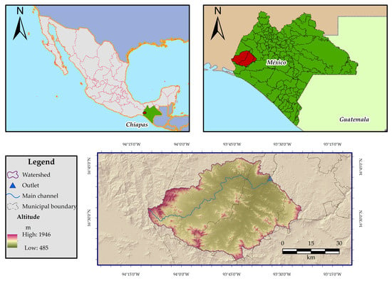
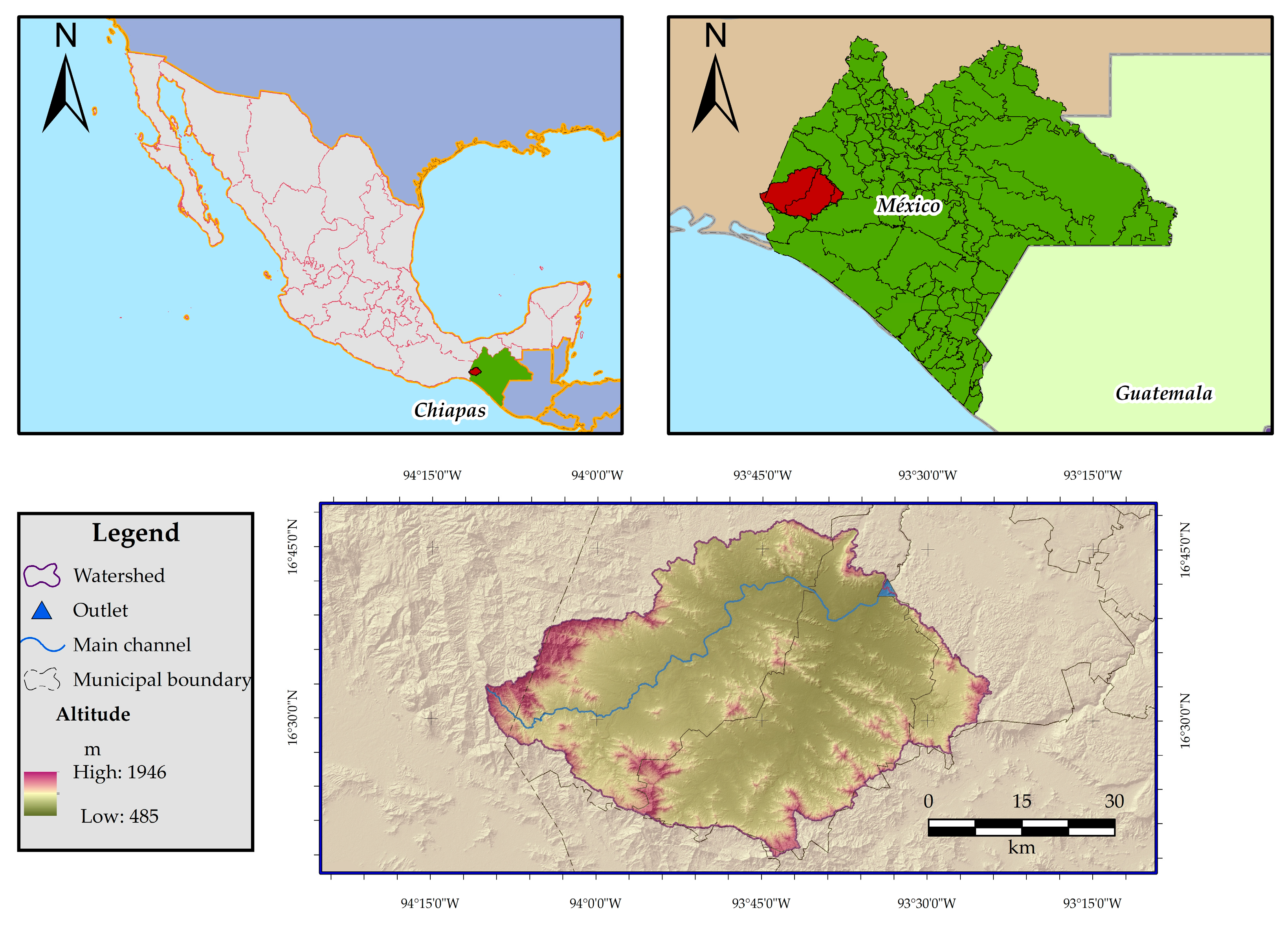
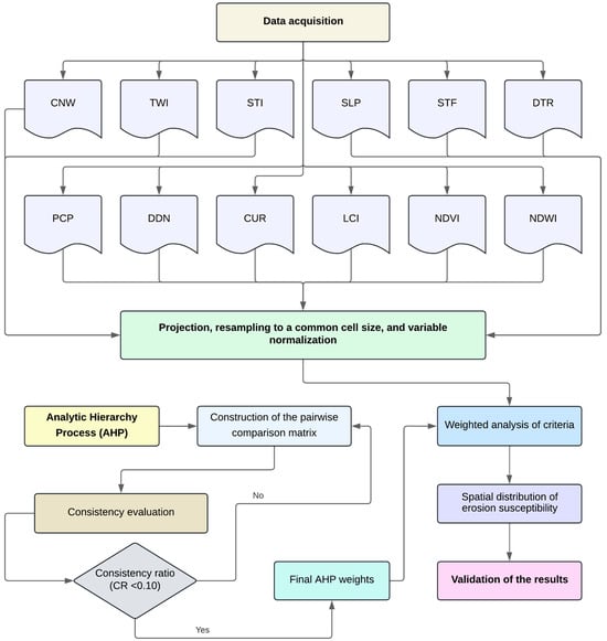
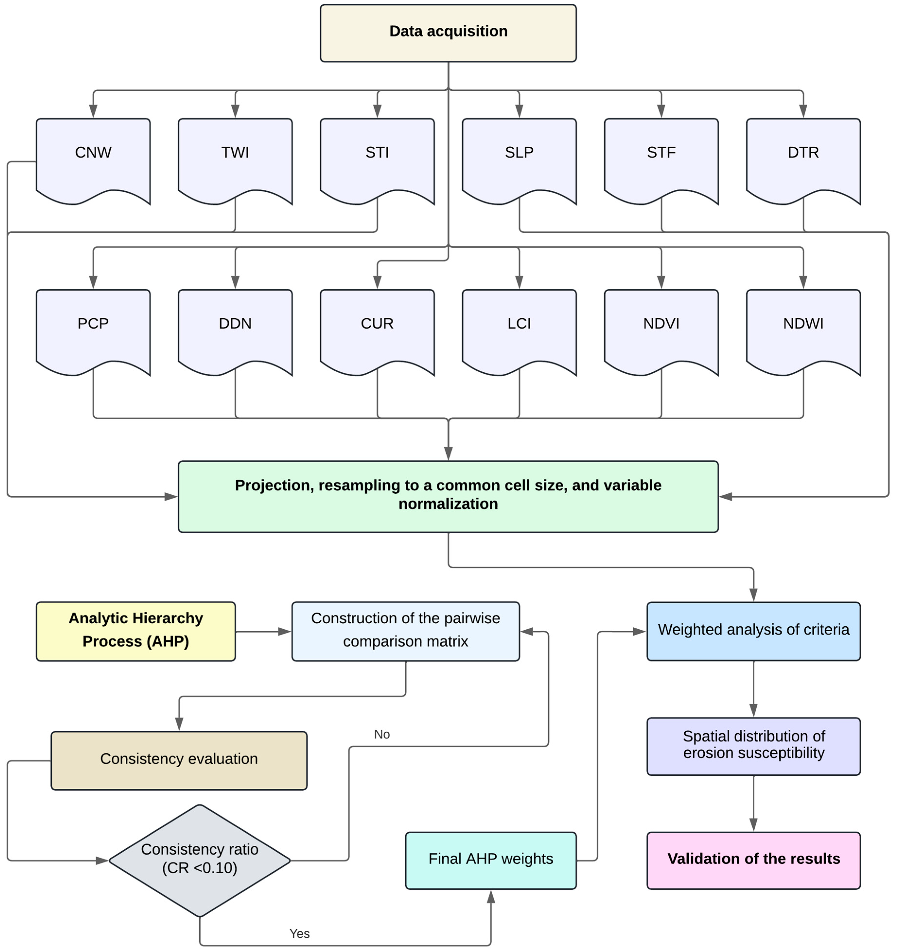
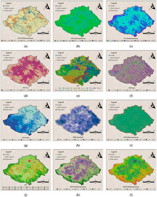
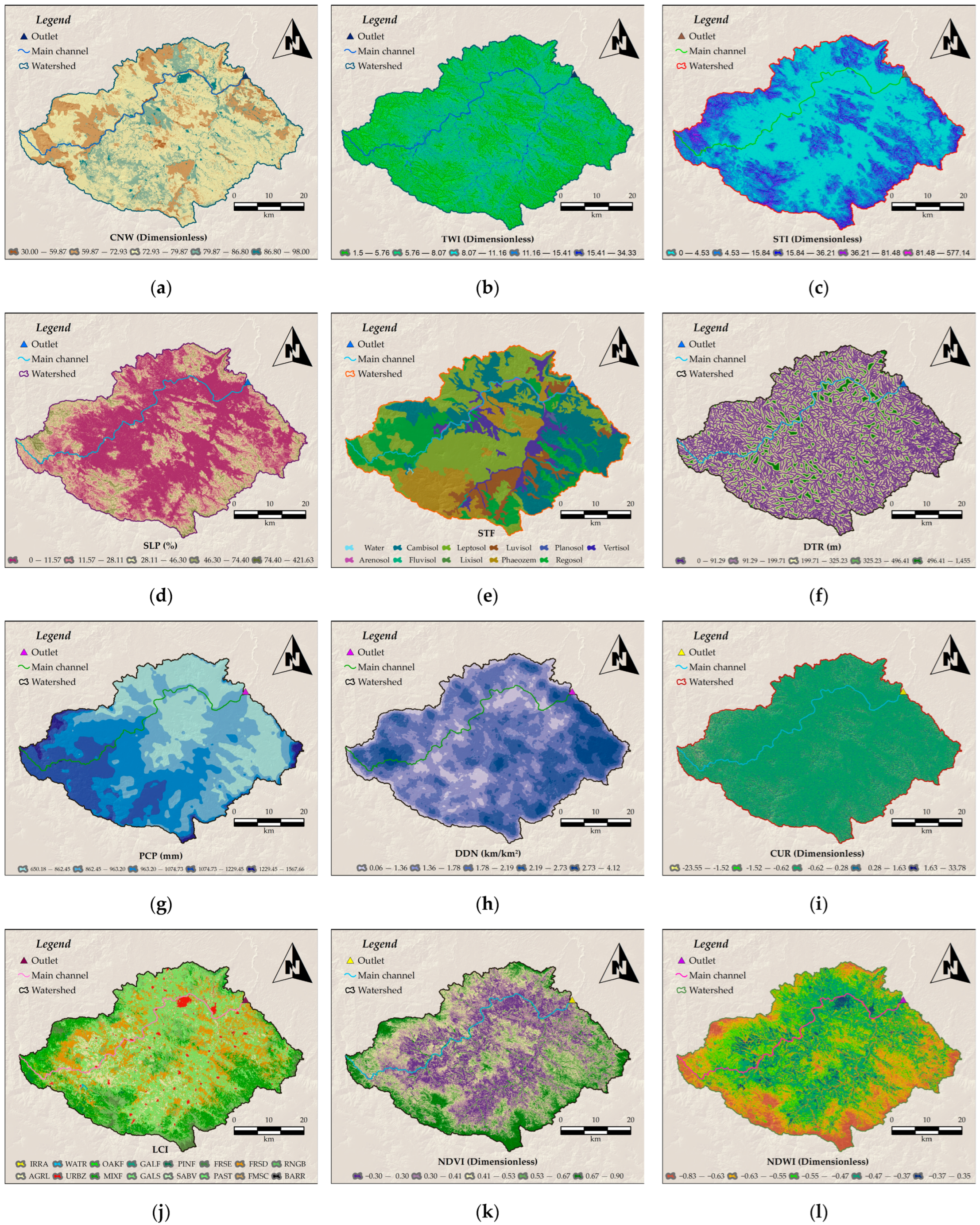
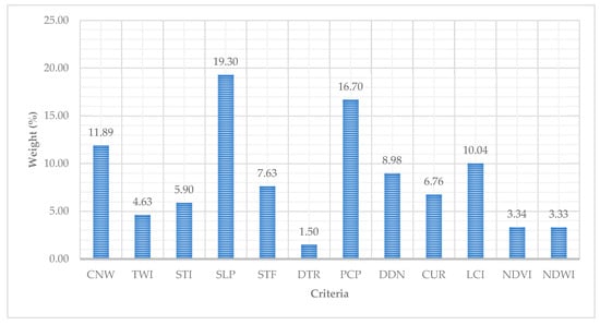
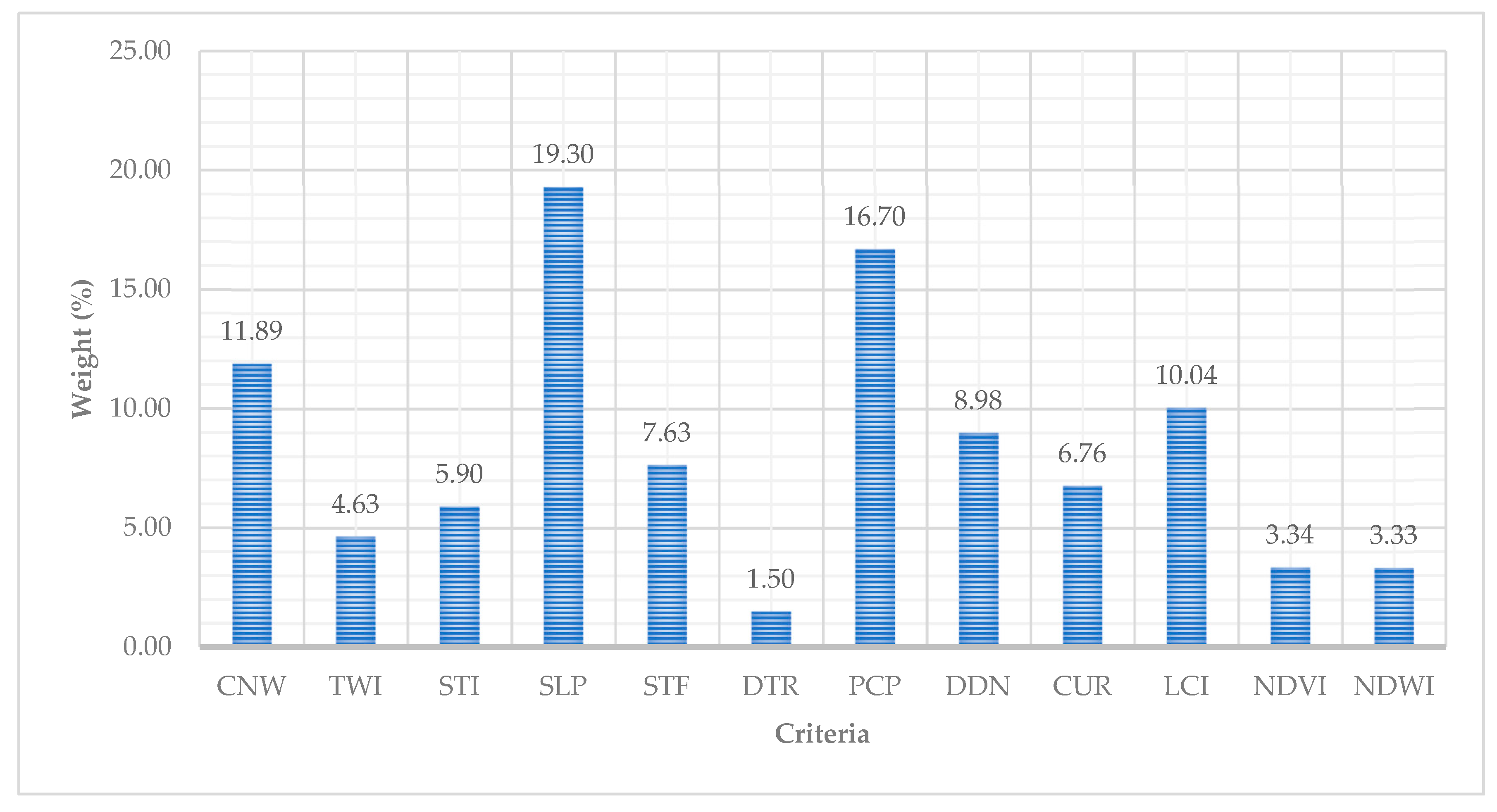
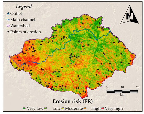
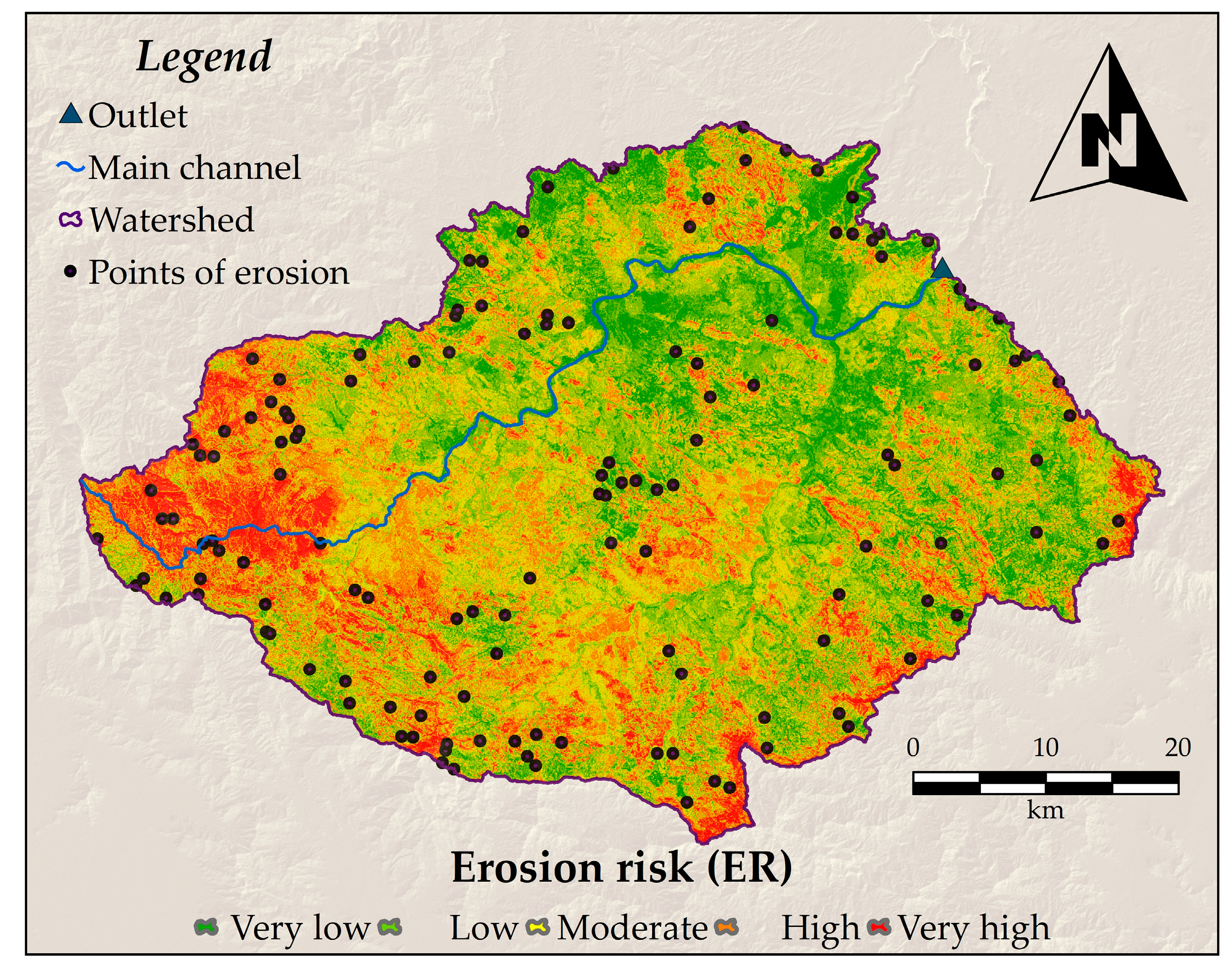
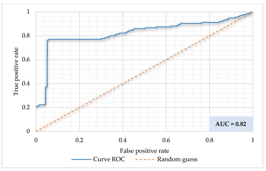
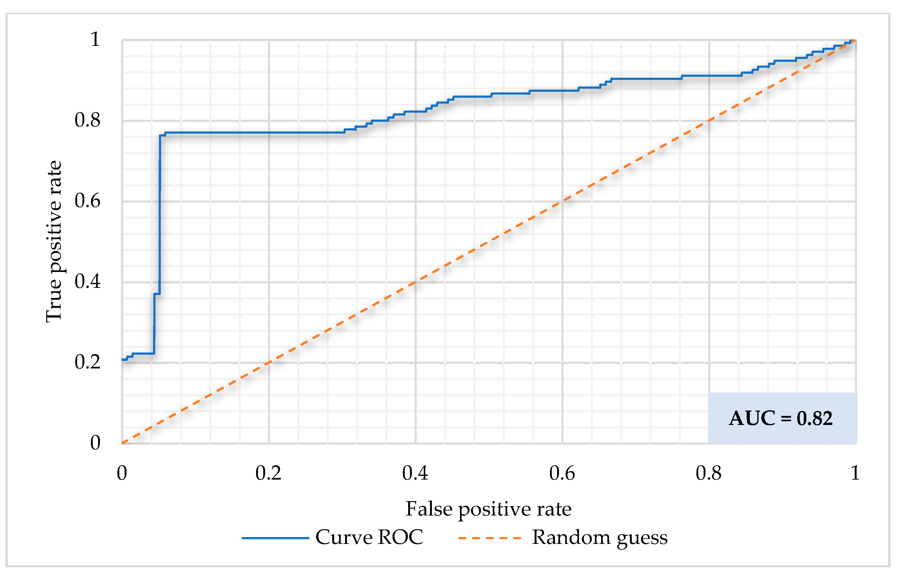

Disclaimer/Publisher’s Note: The statements, opinions and data contained in all publications are solely those of the individual author(s) and contributor(s) and not of MDPI and/or the editor(s). MDPI and/or the editor(s) disclaim responsibility for any injury to people or property resulting from any ideas, methods, instructions or products referred to in the content. |
© 2026 by the authors. Licensee MDPI, Basel, Switzerland. This article is an open access article distributed under the terms and conditions of the Creative Commons Attribution (CC BY) license.