


Abstract
Traditional hazard assessment often relies on simple spatial overlays of static susceptibility and dynamic rainfall thresholds, ignoring the spatial heterogeneity of geological responses to rainfall. To address this limitation, this study proposes a meteorological hazard assessment and dynamic early warning framework for Nujiang Prefecture, Yunnan Province, driven by heuristic spatial heterogeneity weighting. Specifically, this study introduces an S-T-C (Susceptibility–Rainfall trigger index–Causal-heuristic modulation factor) coupling framework that employs Causal Forest Double Machine Learning (CF-DML) to approximate conditional rainfall–geohazard associations and integrates them with static susceptibility and dynamic rainfall threshold modeling for warning zoning. The framework combines an antecedent effective rainfall threshold model (Antecedent Effective Rainfall Intensity–Duration–Daily Rainfall, EI-D-R) with an AutoGluon-based susceptibility model (AUC = 0.9178), and uses CF-DML as a flexible non-linear estimator to approximate conditional responses modulated by environmental factors. This heuristic adjustment is then incorporated into the S-T-C coupling framework. A retrospective case application shows that at the same observed Probability of Detection (POD = 76.5%), the S-T-C framework produces a more spatially selective warning footprint compared to traditional S-T product coupling, with very low-hazard zones expanding from 32.67% to 70.64% (a relative increase of 116.19%). Rather than claiming validated causal identification, this work illustrates that using CF-DML as an association-based, heuristic spatial-heterogeneity weighting approach can provide a more spatially explicit and retrospectively evaluated basis for geohazard assessment and regional risk management, subject to the data and modeling limitations discussed.
1. Introduction
With the rapid advancement of global urbanization and industrialization, the accumulation of greenhouse gases has caused global warming, which has led to frequent extreme meteorological disasters [1]. As reported by the United Nations International Strategy for Disaster Reduction, about 70% of geohazards in the world are directly induced by heavy rainfall. Such geohazards affect a wide range of areas and have great destructive power. They not only take more than 4000 lives every year, but also cause huge economic losses of up to billions of dollars [2]. Notable examples include extreme rainfall-induced mass disaster incidents, such as the 2024 Eryuan event in Yunnan, China, the 2022 Mianyang event in Sichuan, China, the 2021 extreme rainstorm and flood event in Western Europe, and the 2018 Western Japan event. All of these episodes caused heavy human casualties and property destruction, emphasizing the susceptibility of modern infrastructure under combined extreme weather scenarios [3,4,5,6].
To reduce the catastrophic impact of these mass incidents, the development of high-precision early warning systems has become a top priority. At present, the existing research framework mainly develops along two distinct methodological trajectories. The first paradigm focuses on the use of empirical-statistical formulas to predict the time dimension of geohazard occurrence. The most representative ones are the rainfall intensity–duration (I-D) and cumulative rainfall–duration (E-D) threshold curves, which aim to determine the key meteorological lower limit that triggers slope instability by fitting historical geohazard event catalogs [7,8]. For example, Reference [9] constructed an I-D rainfall threshold model based on the historical geohazard situation in the study area, and systematically assessed the risk situation in the northern mountainous area of Quzhou City; Reference [10] introduced the cumulative rainfall E to construct the EID three-dimensional threshold model, which improved the accuracy and refinement of geohazard early warning. At the same time, the spatial dimension of geohazard prediction is highly dependent on advanced machine learning architectures to accurately refine the spatial pattern of geohazard susceptibility. For example, Reference [11] constructed a support vector machine (SVM) model based on fuzzy clustering, which improved the accuracy of landslide susceptibility zoning in Anze County from 0.785 to 0.957. Reference [12] constructed a Stacking ensemble learning model integrated with frequency ratio feature optimization, which achieved the highest predictive accuracy (AUC = 0.8967) for collapse susceptibility assessment in the Henan section of the right bank of the Yellow River under data-scarce conditions. In addition, GIS and remote-sensing approaches provide important methodological support for spatial susceptibility mapping. Reference [13] used 3S technology (GIS, GPS and RS) and 11 factors to assess debris-flow susceptibility in Changping District, Beijing; SVM outperformed the other three models with an AUC of 0.889, indicating strong adaptability to small-sample data. This provides useful methodological context for GIS/RS-based multi-source spatial analysis in geohazard susceptibility mapping.
However, although the above two paradigms have achieved fruitful results in their respective dimensions, there are still obvious limitations in the practice of collaborative disaster prevention and mitigation. On the one hand, the traditional empirical-statistical rainfall threshold is mostly based on the lumped fitting of wide-area meteorological station data, ignoring the spatial heterogeneity of topography, physical and mechanical parameters of rock and soil, and initial soil moisture content, which can easily lead to warning errors in large-scale early warning [14,15,16]. On the other hand, geohazard susceptibility zoning based on machine learning mostly belongs to spatial static assessment, and relies heavily on historical geohazard event data [2,17,18]; it is difficult to reflect the occurrence law of various geohazards under real-time conditions.
Based on the above background, this study chooses Nujiang Prefecture of Yunnan Province as the research area, and proposes a meteorological hazard assessment and dynamic early warning framework driven by heuristic spatial heterogeneity weighting. It should be noted that the present study inherits, at the methodological framework level, the “susceptibility–rainfall threshold dynamic coupling” paradigm established in Reference [19], which employs the AutoGluon automated machine learning framework to construct a susceptibility evaluation model and combines it with a three-dimensional empirical rainfall threshold model (EI-D-R) to characterize rainfall-triggering conditions. Reference [19] achieved the spatial coupling of these two components through a confusion matrix and hierarchical multiplication method, providing a systematic technical pathway for spatiotemporal early warning of regional geohazards. Building upon this foundation, the present study introduces the Causal Forest Double Machine Learning (CF-DML) framework to estimate the spatially heterogeneous moderating intensity of environmental factors on rainfall–geohazard associations. This framework, based on Robinson’s partially linear architecture, achieves orthogonal inference through a two-stage residualization procedure. It non-parametrically captures the modulation of the rainfall–geohazard association by the geological environment context and transforms the resulting Conditional Average Modulation Effect (CAMoE), treated here as an association-based modulation estimand rather than a validated causal parameter, into a heuristic modulation factor, thereby constructing an S-T-C (Susceptibility–Rainfall trigger index–Causal-heuristic modulation factor) spatial coupling model. Here, “causal-heuristic” is retained only as the algorithm-inspired name of the coupling framework. It denotes heuristic weighting based on conditional associations and does not imply formal causal identification. In contrast to the static multiplicative coupling, the S-T-C model realizes a shift from “uniform threshold coupling” to “environment-condition-dependent dynamic coupling” through the introduction of a data-driven spatially varying weighting mechanism. Furthermore, although Reference [20] established a meteorological geohazard early warning model based on AutoGluon in the Yunnan region, its core methodological contribution focuses on sample optimization strategies and machine learning model accuracy improvement, without involving the introduction of an association-based modulation or spatial-heterogeneity weighting framework. The key innovation of this study, therefore, lies in embedding association-based estimation into the susceptibility–rainfall coupling framework, enabling the early warning model to explicitly characterize the nonlinear modulation of geological environments on rainfall-induced geohazard sensitivity, thereby achieving incremental improvements in both the refinement of early warning zonation and physical interpretability. The outputs of this hazard-based framework will provide scientific support for the improvement of local geohazard prevention and control systems, and play an important role in improving emergency response capacity, reducing geohazard economic losses, and ensuring regional economic and social sustainable development.
In this study, the term “risk early warning” is used in accordance with the operational convention of the Chinese geohazard management authorities [21]. Methodologically, however, our work focuses on hazard assessment, and all mathematical formulations use “hazard index” or “warning level” rather than “risk” in the strict academic sense.
2. Study Area and Dataset
2.1. Study Area
The study area (Figure 1) is situated in the northwestern part of Yunnan Province (98°09′–99°39′ E, 25°33′–28°23′ N), encompassing Gongshan County, Fugong County, Lushui City, and Lanping County. The topography of this region forms part of the longitudinal valley system of the Hengduan Mountains. The northern sector is characterized by higher elevations, while the southern sector exhibits lower elevations. Elevations range from 693 m to 5050 m, generating a pronounced topographic relief. This area features a typical alpine canyon landscape with a well-developed drainage network, through which the Dulong River, the Nujiang River, and the Lancang River flow in parallel. Due to the intense neotectonic movement, the broken rock mass, and the strong river incision and gravity erosion, the terrain slope in the area is mostly within 10–50°. The alpine gorge terrain and dense drainage network in the study area contribute to a fragile geological environment, which is associated with high geohazard susceptibility and hazard levels.
Figure 1.
Geographical location of the study area.
To accurately quantify the impact of complex geological background on geohazard evolution in the region and construct an efficient dynamic early warning model, it is urgent to systematically characterize the geohazard-formative environment and trigger factors in the region. Therefore, this paper comprehensively integrates the multivariate spatial geographic data and long-term meteorological observation data of the region, extracts the static susceptibility factors covering multiple dimensions such as topography, stratigraphic lithology, meteorology and hydrology, and couples them with dynamic rainfall triggering factors, laying a data foundation for subsequent hazard early warning and model training.
2.2. Data Sources and Preprocessing
In this study, three types of data were collected and used:
- Complete compilation of regional geohazards and rainfall-induced geohazards;
- Environmental factor dataset for regional geohazard susceptibility assessment;
- Daily process rainfall station data used to determine the rainfall threshold.
The details are presented in Table 1. The geohazard dataset in this study comprises three distinct rainfall-induced geohazard types: landslides, rockfalls/collapses, and debris flows. These three types are merged into a single category for model construction, and no weight coefficients are assigned to individual geohazard types. To justify this aggregation, a type-specific sensitivity analysis is conducted and presented in Section 4.6.
Table 1.
Source of factor data.
All spatial data were preprocessed and resampled to a uniform 200 m grid resolution using ArcGIS Pro 3.0 under the China Geodetic Coordinate System 2000 (CGCS2000). Continuous environmental variables (e.g., elevation, slope) were resampled using bilinear interpolation to preserve the smooth spatial gradients of these surface-like attributes. Categorical variables (e.g., lithology, land use) were resampled using the nearest-neighbor resampling strategy to preserve the integrity of discrete class units without introducing artificial intermediate values. For the dynamic rainfall inputs, forecast daily rainfall was provided by the Yunnan Provincial Meteorological Bureau as an operational gridded product at 1 km resolution. This product is generated by integrating multi-source observations (surface stations, radar, and satellite) with numerical weather prediction and nowcasting systems. At present, 1 km is the most reliable operational resolution available for the study area. Observed rainfall from 3375 meteorological stations (Figure 2) was interpolated using ordinary kriging to the same 1 km grid as the forecast rainfall, because the effective rainfall calculation combines antecedent observed rainfall and current-day forecast rainfall in the same grid cell. The 1 km rainfall grids were then resampled to the 200 m analysis grid only for spatial alignment with static environmental covariates; this resampling does not generate finer meteorological information. Kriging validation statistics are reported in Section 4.3. Missing values in environmental covariates were handled using nearest-neighbor interpolation. Regarding rainfall records, periods with missing data were excluded from the analysis, and the estimation relied solely on the available recorded rainfall data.
Figure 2.
The distribution of rainfall stations.
3. Methodology
This section mainly describes the methodological workflow of this study, and the details are shown in Figure 3. To clarify the terminology used throughout this study, the proposed heuristic (hereafter interpreted as heuristic, association-based) coupling framework is abbreviated as the S-T-C model (Susceptibility–Rainfall trigger index–Causal-heuristic modulation factor), while the traditional benchmark method is denoted as the S-T model (Susceptibility–Rainfall trigger index product coupling).
Figure 3.
Methodological workflow of this study.
3.1. Susceptibility Modeling Based on AutoGluon and Ensemble Learning
In geohazard meteorological early warning systems, the refined evaluation of geohazard susceptibility is the cornerstone and spatial precondition for constructing a spatiotemporal dynamic early warning model. This study adopts AutoGluon [22,23], an advanced automated machine learning (AutoML) framework, as the primary methodology for susceptibility modeling. This framework largely reduces the heavy reliance of traditional machine learning on manual hyperparameter tuning. Specifically, AutoGluon integrates seven distinct algorithm families tailored for tabular spatial data: Gradient-Boosted Decision Trees (CatBoost, LightGBM, XGBoost), Tree-based Ensembles (ExtraTrees, RandomForest), and Deep Neural Networks (NeuralNetTorch, NeuralNetFastAI). Through advanced strategies such as multi-layer stacking (Figure 4), it systematically trains multiple heterogeneous base models and automatically synthesizes a weighted ensemble predictor. Consequently, this architecture can improve the precision and robustness of susceptibility prediction in the present data setting.
Figure 4.
AutoGluon multilayer stack integration diagram.
To objectively evaluate the performance and applicability of AutoGluon in geohazard susceptibility modeling, this study introduces three widely used traditional ensemble learning strategies—Bagging, Boosting and Voting [24,25,26]—as comparison baselines. The Bagging strategy constructs multiple independent base learners by bootstrap self-sampling the original training set, and finally the prediction is aggregated by averaging. The Boosting strategy adopts a sequential training mechanism. Each iteration adjusts the sample weight according to the fitting residuals of the previous round, so that the subsequent learners gradually focus on the samples that are difficult to predict correctly. The final model is expressed as a weighted combination of base learners, which can reduce the prediction bias. The Voting strategy directly trains multiple heterogeneous base models in parallel, and fuses the probabilities of various categories through soft voting, so as to take into account the biases of different algorithms toward the data space and improve the overall robustness. In this study, the Bagging strategy uses decision tree (DT) as the base learner, the Boosting strategy uses gradient boosting decision tree (GBDT) as the base learner, and the Voting strategy uses logistic regression (LR), Extreme Gradient Boosting (XGB), GBDT, and random forest (RF) as the base learners [27,28]. The above four integrated models are trained and optimized using the same feature set, which together constitute comparison baselines for evaluating the effectiveness of AutoGluon.
where represents the geohazard susceptibility index of the evaluation unit calculated using the three ensemble strategies; x denotes the multi-dimensional feature vector composed of hazard-inducing environmental factors; N, S and M correspond to the total number of independent base learners constructed in parallel, the maximum number of iterations in sequential training, and the total number of heterogeneous base models participating in joint decision-making for the three strategies, respectively; denote the outputs of the base learners under each respective strategy; and are the corresponding ensemble weight coefficients.
3.2. Critical Rainfall Threshold Model
To characterize the non-linear response of geohazard occurrence to precipitation, statistical methods were applied to establish empirical critical rainfall thresholds. In view of the current research trend of incorporating antecedent effective rainfall into threshold modeling [29,30], this paper proposes and adopts a multi-factor coupling threshold model, referred to as the EI-D-R model (Antecedent Effective Rainfall Intensity–Duration–Daily Rainfall), which integrates antecedent effective rainfall intensity (EI, mm/d), rainfall duration (D, d), and forecast daily rainfall (R, mm) to support geohazard prevention and early warning.
Antecedent effective rainfall is calculated based on the observed historical rainfall (R1 to Rn) and forecasted daily rainfall (R0) using a decay coefficient. In this study, the decay coefficient αd is taken as 0.8 [20]. This value was not independently calibrated or optimized in the present study, and a systematic sensitivity analysis of αd was not performed; the resulting thresholds should therefore be regarded as conditional on this choice. The widely used method is the power-law approach proposed by Crozier [31] in 1986, and the calculation formula is as follows:
where ER represents antecedent effective rainfall (mm), EI represents antecedent effective rainfall intensity, R0 denotes the forecast daily rainfall on the current day, which is not decayed, Rn denotes the observed daily precipitation n days prior to the event, D denotes the rainfall duration, is the decay coefficient, and n specifies the antecedent duration, which is set to 15 days in this study. Although the term “antecedent” is retained for consistency with previous studies, ER in this study includes both the current-day forecast rainfall R0 and the antecedent observed rainfall R1–R15. Both observed and forecast rainfall are matched on the same 1 km grid before combination.
In this study, we define a rainfall event as a continuous precipitation period corresponding to geohazard induction. This is an operational rainfall-event definition. The onset of such an event is defined as daily precipitation exceeding 5 mm, and it is deemed to have concluded when daily precipitation falls below 5 mm for two consecutive days [20]. Alternative event definitions and threshold values were not tested; the event identification and subsequent threshold results are therefore conditional on this operational definition. Multiple geohazards triggered by the same precipitation process at the same location are consolidated and recorded as a single event. The detailed calculation methodology is illustrated in Figure 5.
Figure 5.
Rainfall duration diagram.
Utilizing historical precipitation records, an empirical and retrospective EI-D-R rainfall threshold model for the study area was derived by integrating three key parameters (EI, D, R). According to the empirical relative-frequency distribution characteristics of the curve, parameter combinations for each relative-frequency grade were extracted at 0.1 intervals, and a nonlinear regression model was subsequently fitted using a modified Sigmoid function. These grades are empirical relative-frequency grades, not calibrated occurrence probabilities. This procedure yielded a three-dimensional continuous empirical threshold surface incorporating EI, D, and R. Based on the rainfall data for each grid unit, the rainfall trigger index T was then computed using the following fitting formula:
where T is the rainfall trigger index (a relative measure of meteorological driving force derived from the EI-D-R model, rather than a strict occurrence probability), D is the rainfall duration, R is the forecast daily rainfall, EI is the antecedent effective rainfall intensity of the previous period, a0 is the intercept, and a1 to a6 are the regression coefficients of the equation.
3.3. Meteorological Hazard Assessment for Spatiotemporal Early Warning Modeling
In this section, two coupling strategies—the traditional product coupling (S-T) and the proposed heuristic dynamic hazard coupling (S-T-C)—are introduced and compared retrospectively.
3.3.1. Hierarchical Multiplicative Coupling (S-T)
In the comparative study of meteorological hazard early warning assessment, the traditional product coupling method is used as the benchmark. Under a unified spatial reference framework, this method applies map algebra to multiply the static susceptibility index (S) grid by pixel with the dynamic rainfall trigger index (T) grid, so as to construct the dynamic hazard index (P) grid.
where S is the susceptibility index, which characterizes the spatial difference in static geological conditions; T is the rainfall trigger index on a specific date; P is the hazard index under the traditional product coupling method. S and T are divided into five levels, and the corresponding level intervals are multiplied to divide the study area into five types of very low to very high warning areas. The threshold division is shown in Table 2.
Table 2.
Multiplication geohazard warning zoning classification.
3.3.2. Causal-Heuristic Dynamic Hazard Coupling (S-T-C)
This study proposes a hybrid dynamic hazard assessment method that integrates geohazard susceptibility with rainfall trigger index. Specifically, Double Machine Learning (DML) was adopted to estimate the association-based Conditional Average Modulation Effect (CAMoE) of geo-environmental variables on rainfall–geohazard associations. This effect, denoted as , represents the change in the conditional expectation of hazard occurrence associated with a one-unit shift in the rainfall trigger index, holding the static geological background constant for each grid cell. This is a conditional association estimand, not a validated causal effect. It is subsequently embedded into a multiplicative hazard-coupling framework to capture the spatially heterogeneous modulating strength of environmental background on the rainfall-hazard association. is an association-based estimand that serves as a data-driven weighting function, not a validated causal parameter, and thus refers to it as a “causal-heuristic modulation factor” only in the heuristic, association-based sense throughout the text. The overall data-driven workflow of the proposed CF-DML dynamic hazard assessment framework is schematically illustrated in Figure 6.
Figure 6.
Overall data-driven workflow of CF-DML framework. Note: The term “causal-heuristic” refers to the heuristic coupling strategy used in the framework and does not imply formal causal identification.
Prior to modeling, environmental covariates are preprocessed for feature construction: two categorical covariates (land use and lithology) are one-hot encoded, with one reference category dropped for each to avoid the dummy-variable trap. The continuous variables are discretized via equal-interval binning, while the remaining covariates are treated as continuous variables and standardized using z-score transformation, without discretization or one-hot encoding. The final constructed feature matrix X contains a total of 18 covariates. The static geohazard susceptibility component is generated by a pre-trained AutoGluon automated machine learning framework, which leverages multi-layer stacking and multi-model ensemble strategies to output spatial hazard probabilities.
To quantify the association between the rainfall trigger index and hazard occurrence, a Causal Forest Double Machine Learning (CF-DML) framework is used [32,33]. Based on Robinson’s partially linear architecture [34], this framework performs orthogonalized estimation via a two-stage residualization technique. The baseline mathematical formulation is defined as:
where Y is the outcome variable indicating geohazard occurrence, T is the treatment variable indicating rainfall-induced geohazard occurrence, represents the CAMoE, g(X) and are the non-parametric conditional expectation functions of the confounding factors, and and denote the idiosyncratic error terms.
To handle nonlinear confounding within the discretized feature space, XGBoost regressors [35] with a squared error loss function are utilized. The algorithm’s built-in regularization and sparsity-aware structure not only navigate high-dimensional sparse matrices but also provide the residualization required for orthogonalized estimation. Moreover, its tree-based nature provides a coherent methodological bridge to the subsequent causal-forest-based estimation of CAMoE. A two-stage cross-fitting strategy is employed to strip away structural confounding from environmental factors, yielding the orthogonal residuals of the outcome and the treatment , thereby mitigating regularization bias. In the second stage, the causal forest performs honest splitting by maximizing the spatial heterogeneity of the orthogonal residual scores to resolve highly heterogeneous effects at individual spatial units without parametric assumptions. At a target pixel x, the non-parametric estimation of CAMoE is formulated as:
where represents the non-parametric sample estimator of the underlying target parameter evaluated at pixel location x, and are the outcome and treatment orthogonal residuals for the i-th sample, respectively, and N is the total sample size. The term denotes the local similarity weights adaptively computed by the causal forest based on environmental feature proximity, quantifying the weighted contribution of neighboring observations to the target evaluation unit x. This mechanism provides a non-parametric mapping from the global Average Modulation Effect (AMoE) to pixel-scale spatially heterogeneous effects (CAMoE).
To synthesize susceptibility, rainfall trigger index, and heuristic modulation factor into a unified hazard index—which is further classified into five warning levels using the natural breakpoint method—we adopt the following heuristic coupling framework:
where P(x) denotes the coupled dynamic geohazard warning index at spatial location x, S(x) represents the susceptibility probability estimated by AutoGluon, T(x) denotes the dynamic rainfall trigger index, is the logistic function, is a scaling factor governing the sensitivity of the adjustment to the CAMoE estimate , and ∈ [0, 1] is the modulation parameter that determines the maximum deviation of the rainfall exponent from unity.
The rationale for this formulation is as follows. The baseline product S(x)T(x) already embeds the geological environment’s influence through S(x), which encapsulates the long-term spatial controls on hazard occurrence. The CF-DML-derived τ(x) represents the estimated additional, environment-dependent modulation of the rainfall–geohazard association beyond what is already represented by S(x). Since 0 < T(x) < 1 and q(x) > 0, the exponent q(x) = 1 + α[1 − 2σ(kτ(x))] directly determines, by its relative position to 1, the direction of adjustment applied to the rainfall contribution. Here α is constrained to 0 < α < 1, so that q(x) > 0 and the coupling remains bounded. Specifically, when τ(x) > 0, we have σ(kτ) > 0.5, so q(x) < 1; because the base T(x) lies between 0 and 1, it follows that T(x)q(x) > T(x), resulting in a heuristic amplification of the rainfall component. Conversely, when τ(x) < 0, we have σ(kτ) < 0.5, so q(x) > 1, which yields T(x)q(x) < T(x), thus producing an attenuation of the rainfall contribution. Therefore, this transformation maps positive and negative CAMoE values into upward and downward adjustments of the rainfall contribution, respectively, serving as a bounded weighting mechanism rather than a re-modulation of the geological information already embedded in S(x). This sign-based interpretation is qualitative and is not intended to imply that Equations (14) and (15) are derived from the DML structural equations. It should be emphasized that this weighting rule provides only a heuristic adjustment in terms of relative intensity and does not yield a calibrated hazard probability or a deterministic hazard estimate. The factor α controls the maximum intensity of this adjustment, with α = 0 degenerating to the conventional multiplicative model S(x)T(x). We emphasize that this coupling equation is heuristic—it is designed as a practical weighting scheme to refine warning boundaries rather than a probabilistically derived hazard model. It is not derived from the DML structural equations, nor does it claim to produce a calibrated conditional hazard probability.
The parameters k and α were set as reference values and examined in a sensitivity analysis, with detailed procedures and results presented in Section 4.6.
3.4. Model Accuracy Metrics
The prediction results of each model were evaluated using the ROC curve and confusion matrix. The Receiver Operating Characteristic (ROC) curve is recognized as a standard method for assessing the overall performance of machine learning models [36]. A curve that bends more closely toward the upper-left corner indicates stronger predictive performance. The area under the ROC curve, defined as the AUC, quantifies the classifier’s discriminative ability, with higher AUC values reflecting superior classification performance.
In addition to the ROC curve, balanced accuracy, precision, recall, and F1 score were adopted as supplementary metrics to facilitate a comprehensive model evaluation. The calculation formulas for the above relevant indicators are presented as follows:
where Balanced-Accuracy refers to the average classification accuracy across all sample categories, Precision quantifies the proportion of correctly predicted positive samples among all positive predictions, Recall measures the fraction of actual positive samples that are correctly identified, and the F1 Score represents the harmonic mean of these two metrics. These metrics should be read together with the spatial block cross-validation design and the associated limitations.
3.5. Model Interpretability Based on the SHAP Framework
To strike a balance between local attribution accuracy and global explanatory consistency, the SHAP (SHapley Additive exPlanations) framework is introduced, which applies the Shapley value from cooperative game theory to quantify the contribution of individual features to the model output [19,37]. In machine learning applications, each input feature contributes to the model prediction. The SHAP value quantifies the average marginal contribution of a given feature across all possible feature subsets.
In practice, this methodology decomposes the predicted value of an individual sample and maps it onto respective feature dimensions. By computing these feature-specific SHAP values, the driving effect of each variable on the final prognostic output can be mathematically isolated, thereby facilitating a rigorous quantitative attribution analysis. The SHAP value of feature i is expressed as:
where F constitutes the entire feature space; S represents a feature subset cleared of feature i; denotes the expected prediction yielded by subset S; and operates as a scaling factor designed to neutralize the mathematical bias induced by varying subset dimensions.
4. Results
4.1. Correlation Analysis
Correlation analysis was used to reduce potential multicollinearity among environmental factors (Figure 7). It can be seen that the elevation is highly correlated with the road density, and the slope is strongly correlated with the relief amplitude. The correlation coefficient between the two is more than 0.5. Therefore, road density and relief amplitude were excluded as a modeling choice to reduce collinearity, and nine factors including elevation, normalized difference vegetation index (NDVI), drainage density, plan curvature, slope, aspect, land use, lithology and distance to fault are selected for susceptibility evaluation (Figure 8), in which lithology is classified into five engineering rock groups based on mechanical strength: I (Hard Massive Rock Group), II (Hard Stratified Rock Group), III (Moderately Hard Stratified Rock Group), IV (Soft Stratified Rock Group), and V (Unconsolidated Deposit Group). A sensitivity analysis in which road density and relief were re-included was not performed; therefore, the selected factor set is not claimed to be unique or optimal. The susceptibility results and subsequent warning zonation should be interpreted as conditional on this selected covariate set.
Figure 7.
Correlation coefficient between environmental factors.
Figure 8.
Environmental factors: (a) elevation (m); (b) NDVI; (c) aspect (°); (d) slope (°); (e) drainage density (km/km²); (f) plan curvature; (g) land use; (h) distance to fault (m); (i) lithology.
4.2. Hyperparameter Optimization
To benchmark AutoGluon against conventional ensemble learning, we selected three representative paradigms—voting, bagging, and boosting—for comparison. All models were developed and evaluated under an identical spatial leave-one-group-out cross-validation (LOGO-CV) procedure. The study area was divided into five spatial groups; in each iteration, one spatial group was held out as the test set and the remaining four groups were used for training. This constitutes a five-fold spatial group cross-validation. This design reduces the spatial dependence between training and test observations and provides a more spatially conservative evaluation than random or stratified partitioning.
For the traditional strategies, base-learner hyperparameters were systematically optimized via Bayesian optimization. In contrast, AutoGluon was configured with the best_quality preset, while all other hyperparameters remained at their defaults. Under this configuration, AutoGluon automated both hyperparameter tuning and model architecture selection using a multi-layer stacking scheme with leave-one-group-out cross-validation bagging to curb overfitting.
For the first-stage residualization within the CF-DML framework, XGBoost regressors were employed as base estimators and systematically tuned using Bayesian optimization to construct the outcome nuisance model and the treatment nuisance model. CF-DML is used here as an association-based modulation estimator rather than a validated causal identification procedure. In the second stage, the CF-DML estimator was initialized using the optimal Model_Y and Model_T as base learners. To handle the continuous rainfall trigger index, discrete_treatment was set to False. The causal forest architecture was configured with 200 trees (n_estimators = 200) and a maximum tree depth of 5 (max_depth = 5), with standard automated covariance inference enabled (inference = ’auto’), while all other hyperparameters remained at their defaults.
The hyperparameter search intervals and calibrated optimal parameters for all the base models and the CF-DML nuisance models are summarized in Table 3.
Table 3.
Hyperparameter search ranges and optimal values of baseline models.
4.3. Rainfall Threshold Modeling and Analysis
Based on the ArcGIS Pro platform, the spatial discretization of the study area is divided into 200 m grid units to form a unified spatial analysis base map. On this basis, the rainfall trigger factors were introduced and extracted pixel by pixel, including rainfall duration D, forecast daily rainfall R and antecedent effective rainfall intensity EI. These variables were derived from historical rainfall records associated with recorded geohazards through spatial interpolation, and were assigned to each grid unit by spatial interpolation to ensure the spatial consistency of the samples and the effectiveness of statistical analysis. To evaluate the kriging interpolation performance, validation statistics were computed for four representative rainfall events (Table 4). The mean error (ME) ranged from−0.0231 to 0.0039 mm, the root mean square error (RMSE) from 0.8632 to 9.9482 mm, the root mean square standardized error (RMSSE) from 0.8795 to 0.9182, and the coefficient of determination (R2) from 0.2740 to 0.7268. The 90% and 95% interval coverage rates were 92.17–96.47% and 95.18–97.48%, respectively, slightly above nominal levels. These statistics indicate limited systematic bias and uncertainty estimates close to nominal levels for these events. However, R2 varied considerably across events and was low for some events, and the coverage rates were slightly above nominal levels; therefore, the interpolation uncertainty should not be regarded as uniformly low. As described in Section 2.2, the 1 km rainfall grid is the operational resolution at which observed and forecast rainfall are matched. Resampling to the 200 m analysis grid does not generate finer meteorological information, and the 200 m rainfall input should be interpreted as a regional rainfall background rather than a locally precise value. A sensitivity analysis across rainfall resolutions was not feasible because only the 1 km operational forecast product was available. The subsequent threshold results are therefore conditional on this operational 1 km resolution.
Table 4.
Kriging validation statistics for representative rainfall events.
Using a multiple regression modeling method, a three-dimensional rainfall threshold model with EI, D and R as explanatory variables was finally constructed. The fitting equation is as follows:
Model fitting performance and predictive accuracy were evaluated using the coefficient of determination (R2), mean squared error (MSE), and mean absolute error (MAE). The fitting surface and accuracy metrics are presented in Figure 9 and Figure 10, respectively. The results indicate an R2 value of 0.9848, implying that D, R, and EI collectively account for 98.48% of the variance in T, indicating high explanatory capacity for the training dataset. The low error metrics (MSE = 0.0013, MAE = 0.0275) indicate only minor deviations between predicted probabilities and observed values, which suggests a good overall model fit.
Figure 9.
Three-dimensional dynamic rainfall threshold surface.
Figure 10.
Rainfall threshold model fitting effect diagram: (a) comparison plot of actual and predicted cumulative probabilities; (b) residual plot of the predictive model.
4.4. Evaluation of Four Susceptibility Models
In this study, a 500 m random sampling strategy outside the buffer zone was used to construct a positive and negative sample data set. The grid unit of historical geohazards is used as a positive sample, and an equal or specified number of non-geohazard grids are randomly selected in the area outside the 500 m buffer zone around the geohazard point as a negative sample for the susceptibility evaluation model. To ensure a fair and robust comparison across different algorithms, all models were developed and evaluated under the same spatial leave-one-group-out cross-validation (LOGO-CV) procedure. The study area was divided into five spatial groups; in each iteration, one spatial group was held out as the test set, and the remaining four groups were used for training. The prediction performance of multiple models was compared by experiments, including the optimal model obtained by automatic training and screening using the AutoGluon automatic machine learning framework—which internally generated 218 distinct model instances across two stacking layers (L2 and L3) with an average training time of 1545.15 s per fold—and three ensemble models based on Voting, Bagging and Boosting.
The evaluation metrics of the four models are summarized in Figure 11 and Table 5. All metrics were computed from the pooled out-of-fold predictions. AutoGluon achieved the highest AUC (0.9178), AP (0.9051), balanced accuracy (0.8600), recall (0.8864) and F1 score (0.8585). Its precision (0.8378) was slightly lower than that of Bagging (0.8420) and Voting (0.8440). Within this validation design, all models achieved an AUC of at least 0.9000 and an F1 score of at least 0.8400, indicating relatively high category discrimination ability for the present sample. The results of susceptibility mapping were divided into five grades according to the natural breakpoint method, as shown in Figure 12. In summary, AutoGluon showed a relatively better overall performance than the other three traditional ensemble models under the default configuration for this dataset, while all models exhibited comparable discriminative ability within the present evaluation setting. These results suggest that the automated ensemble method can provide a useful basis for susceptibility mapping under the present data and modelling constraints, but they do not validate its general spatial predictive performance. Furthermore, the five-grade susceptibility zonation provides a spatially explicit representation of susceptibility that can support subsequent hazard assessment, subject to the spatial validation design and the limitations discussed in this study.
Figure 11.
Model evaluation curve: (a) ROC curve; (b) PR curve.
Table 5.
Comparison of model accuracy evaluation indexes.
Figure 12.
Susceptibility zoning mapping.
4.5. Evaluation of Double Machine Learning Models
The sample set in this study was constructed using positive and negative cases of geohazards in a 1:1 ratio. The positive cases were directly taken from the 204 historical rainfall-induced geohazard events and their corresponding dates recorded in the study area, and the negative cases were generated according to the following rules: Taking each positive case date as a reference, a low rainfall date with daily rainfall less than 5 mm and cumulative rainfall less than 20 mm in the preceding 15 days was screened in the time window of 7 days before and after it, and a date satisfying the above conditions was randomly matched for each positive case, and an equal number of random spatial points were generated within the boundary of the study area. Subsequently, individual points with daily rainfall less than 1 mm and antecedent effective rainfall (ER) exceeding the 95% quantile of positive ER, or rainfall duration of 1 day and abnormally high ER, were excluded to improve the typicality of negative cases. These negative cases are synthetic pseudo-absence controls rather than verified non-event observations; they therefore cannot be used to estimate operational false-alarm rate, specificity, precision, or related early warning metrics. In this study, the CF-DML framework was used to estimate conditional, association-based modulation of rainfall-related factors on geohazard occurrence under the case–control sampling design, and the model performance was evaluated in terms of numerical consistency, spatial heterogeneity, and sensitivity to model specification.
Figure 13 shows the spatial distribution and frequency statistics of CAMoE in the study area. The spatial AMoE (0.1843), defined as the regional mean of grid-scale CAMoE estimates, represents the estimated average change in the conditional expectation of geohazard occurrence associated with a unit increase in the rainfall trigger index while holding the geological background constant in the model; it is an association-based modulation estimand, not a validated causal effect or a calibrated probability change. Lying near the center of the CAMoE distribution, this value represents the overall average marginal effect of rainfall on geohazard occurrence at the regional scale. To assess model-based uncertainty in grid-scale estimates, we derived 95% confidence intervals (CIs) for each pixel using the CF-DML inference framework. The average pixel-level CI across the entire study area is [0.0194, 0.3493], with a mean interval width of 0.3299. The lower bound of this average CI is well above zero, indicating a significantly positive overall marginal effect of rainfall at the regional scale. Furthermore, 63.75% of all pixels exhibit CIs that do not cross zero, indicating that the vast majority of the region shows a statistically discernible rainfall-modulation effect. This high proportion of significant estimates, together with the consistently positive average CI, suggests a predominantly positive conditional association in the fitted model on geohazard susceptibility across most of the study area, while the remaining pixels display relatively smaller effect magnitudes that are statistically indistinguishable from zero but remain within the expected range of spatial variability. In contrast, the training set AMoE (0.3451) was substantially higher and lies in the upper quantile of the CAMoE distribution. This discrepancy arises from the 1:1 case–control sampling design, which over-represents units with high baseline geological susceptibility. Such high-susceptibility units exhibit a much stronger marginal response to rainfall than the regional average, indicating pronounced spatial heterogeneity in the estimated modulation patterns.
Figure 13.
Distribution of CAMoE in the study area. (a) spatial distribution; (b) frequency distribution and statistical summary.
In addition, under a series of robustness tests (Figure 14), such as placebo replacement test (p < 0.001), multi-threshold binarization (25th, 50th, 75th quantiles), replacement of random forest as the nuisance model and quantile transformation, the sign of the estimated association remains consistent and is statistically distinguishable from zero under the present inferential setting. The above test results indicate that the direction of the estimated rainfall association was consistent across the tested specifications.
Figure 14.
Results of the robustness test: (a) placebo test histogram; (b) robustness checks for the average modulation effect (AMoE) under different model specifications.
4.6. Sensitivity Analysis
Prior to evaluating the stability of the S-T-C framework, the reasonableness of aggregating three geohazard types—landslides, rockfalls/collapses, and debris flows—was examined through a type-specific sensitivity analysis. Each type was combined with the same set of negative samples and modeled independently using the same Boosting algorithm as the main model. The prediction performance and permutation-based feature importance were compared across the three types. The results (Figure 15) show that the three types achieved comparable performance (AUC = 0.914, 0.964, and 0.924 for collapses, debris flows, and landslides, respectively), and their feature importance rankings were moderately to strongly correlated (Spearman ρ = 0.650–0.817), with elevation consistently identified as the largest SHAP attribution in the fitted model. These findings suggest, under the present type-specific comparison, that the three geohazard types share a broadly comparable set of controlling factors and can be treated as a combined category for regional-scale susceptibility modeling.
Figure 15.
Performance and feature importance comparison among the three geohazard types.
Having examined the reasonableness of the type aggregation, we then assessed the sensitivity of the proposed S-T-C dynamic warning coupling framework. A sensitivity analysis was conducted on the exponent modulation parameter α and the Sigmoid scaling factor k. In this evaluation, was systematically varied across the interval [0.1, 1.0] around its reference value of 0.5, while k was scanned across [0.1, 2.0] around its reference value of 1.0. The area fractions of the five classes (Very Low, Low, Medium, High, and Very High) were tracked as response metrics to evaluate the sensitivity of spatial warning partitioning to parameter perturbations.
As shown in Figure 16, the spatial distribution of geohazard zoning levels remains relatively stable across the tested parameter ranges. As increases from 0.1 to 1.0, the area proportions for all five zoning level categories remain nearly constant, with the Very Low level consistently accounting for the vast majority of the study area (~71.5–70.0%), followed by Low (~15.0%), Medium (~7.5%), High (~5.0%), and Very High (~2.5%). Similarly, modifying the Sigmoid scaling factor k across [0.1, 2.0] yields nearly flat response profiles across all warning classes. The aggregated proportion of high-hazard regions (High and Very High categories) remains stable at around 7.5%, indicating that, within the tested ranges, the Sigmoid transformation bounds the modulation factor without producing unbounded or erratic changes in the rainfall exponent.
Figure 16.
Sensitivity analysis of susceptibility area fractions under varying S-T-C coupling parameters: (a) response to exponent modulation parameter ; (b) response to Sigmoid scaling factor k. Dashed vertical lines indicate the selected baseline default values ( = 0.5 and k = 1.0).
Overall, these sensitivity profiles indicate that the S-T-C multiplicative coupling structure is relatively insensitive to α and k within the tested parameter ranges under the explored conditions. These values are retained as default/reference settings for consistency with the original framework specification and to avoid introducing additional tuning in the absence of an independent predictive calibration criterion. Independent calibration and validation against observed geohazard records or other predictive performance metrics remain necessary before any optimality claim can be made. Accordingly, α = 0.5 and k = 1.0 are used as baseline reference values in this study, while their predictive optimality remains to be tested in future work.
4.7. Meteorological Hazard Assessment and Early Warning Mapping
To illustrate the performance differences between the two coupling strategies in practical early warning scenarios, this study selected a typical rainfall-induced geohazard event that occurred on 25 May 2020 (Table 6) as a retrospective illustration. This exercise is a retrospective case application, not independent validation of predictive performance, because the same 204-event dataset was used across sequential stages of the analysis and the 2020 events were not excluded from model development. The variables R, D, and EI were extracted for all grid cells within the study area on this date. These parameters were then integrated into the empirical EI-D-R continuous probability rainfall threshold model to calculate the rainfall trigger index (T). Meteorological hazard early warning zonation maps were subsequently generated by combining the spatial susceptibility results using two distinct methods: traditional product coupling (S-T) and heuristic dynamic hazard coupling (S-T-C). The distribution of grid cells across different warning zones was then quantified.
Table 6.
Detailed information on rainfall-induced geohazards.
Figure 17 illustrates the spatial distribution of the rainfall-trigger index and the associated warning zones, while Table 7 summarizes the corresponding statistics by using zonal statistics. Spatial comparison of the results presented in Figure 17 indicates that both coupling methods yield broadly similar macro-scale warning patterns. For the 17 recorded events on 25 May 2020, both methods identified 13 events under the stated warning criterion (Probability of Detection, POD = 76.5%). This POD is calculated only from the 17 recorded events in this retrospective case; it is not an independent validation metric and does not represent operational detection performance. At this same observed POD, the S-T-C method produced a more spatially selective warning footprint than the S-T method in this case. Notably, under an identical detection capability—achieving a POD of 76.5% for the 17 recorded events—a marked divergence emerges in the spatial extent of warning zones. Statistical analysis reveals that while maintaining this equal event detection, the proposed S-T-C method changes the hazard areal proportions compared to the conventional S-T approach. Compared to the conventional S-T approach, the S-T-C method notably expands the very low-hazard area from 32.67% to 70.64%, representing a substantial increase of 37.97 percentage points (a relative expansion of 116.19%). Correspondingly, the areal proportions of the low, medium, high, and very high-hazard zones are reduced to 14.60%, 7.39%, 4.77%, and 2.64%, respectively. With both methods identifying 13 of the 17 recorded events, the S-T-C method compresses the high and very high-hazard warning footprint to a combined area of 7.41%. These findings indicate that, in this retrospective case, the S-T-C coupling strategy produces a more spatially selective high-hazard warning footprint than the traditional S-T model at the same observed POD, without changing the number of detected recorded events. Ultimately, achieving the same number of detected recorded events with a smaller high-hazard footprint provides a potentially useful, retrospectively evaluated basis for regional geohazard prevention, risk mitigation, and resource optimization, subject to the data and modelling limitations discussed in this study.
Figure 17.
Meteorological hazard assessment and early warning zoning ((Left): S-T; (Middle): S-T-C; (Right): Distribution of rainfall trigger index on the day).
Table 7.
Warning zoning statistics for geohazards on 25 May 2020.
4.8. Interpretability Analysis
To evaluate the relative contributions of nine environmental factors to the spatial susceptibility of geohazards and to quantitatively analyze their association-based moderating patterns on rainfall-induced geohazard responses, this study employed the SHAP method following the construction of the susceptibility and rainfall threshold models. By comparing the global SHAP importance of the susceptibility model with the feature attribution values of the CAMoE, the statistical correlations and feature contributions in the fitted model were evaluated for the environmental factors, respectively.
The global SHAP importance statistics (Figure 18) indicate that elevation is the primary factor affecting the spatial distribution of susceptibility (importance value: 0.275), followed by distance to faults (0.046), drainage density (0.041), and slope (0.038). Combined with the results from the SHAP beeswarm plot (Figure 19), the SHAP values for samples with low elevation and short distances to faults are predominantly distributed in the positive range, indicating that lower relative elevation and closer proximity to faults are positively correlated with geohazard susceptibility. The SHAP dependence plots of the core factors (Figure 20) demonstrate nonlinear and threshold relationships between variable feature values and partial effects. Specifically, the SHAP value for elevation (<2500 m) is positive; it subsequently drops below zero and stabilizes as the value increases. For the distance to faults, the magnitude of its negative impact significantly increases once the distance exceeds 2500 m. Drainage density is generally positively correlated with SHAP values, and this effect levels off when the density exceeds 250 km/km2. Conversely, the partial effect of slope exhibits a monotonically decreasing trend. Additionally, the color distribution of the scatter points in the dependence plots indicates the nonlinear interactions among multiple variables.
Figure 18.
Importance of environmental factor characteristics.
Figure 19.
SHAP diagram of susceptibility model.
Figure 20.
SHAP dependence plots for the top four dominant factors: (a) elevation (m); (b) distance to fault (m); (c) drainage density (km/km2); (d) slope (°).
To quantify how static environmental factors are associated with the spatial heterogeneity of CAMoE, a surrogate model (XGBoost) was trained on the estimated association-based modulation effects (CAMoE) and subsequently interpreted using shap.TreeExplainer (Figure 21). The relative contribution of each factor was evaluated via mean absolute SHAP values.
Figure 21.
Feature importance of background factors based on SHAP contribution to CAMoE (Top 10).
The results show that slope (0.0774) and distance to faults (0.0591) are the primary predictors of estimated CAMoE in the surrogate model, indicating that the terrain relief and geological fault structures are strongly associated with spatial variation in the estimated rainfall–geohazard association. Furthermore, lithology (Class III, 0.0409), drainage density (0.0294), elevation (0.0271), NDVI (0.0170), aspect (0.0154), and plan curvature (0.0104) exhibit corresponding association-based moderation effects on CAMoE heterogeneity. The contribution values of grassland (0.0068) and other land use types, as well as the remaining lithological categories, are all less than 0.01, indicating a marginal relative contribution to CAMoE variability within the surrogate framework. In conclusion, the results indicate that the association-based rainfall modulation effect, as estimated within the CF-DML framework, varies across space and is nonlinearly conditioned by site-specific environmental factors. Coupling SHAP attribution with the CF-DML model provides a quantitative basis for retrospectively interpreting hazard associations and refining warning zonation, rather than for validating operational early warning performance.
5. Discussions
5.1. Dataset
The dataset used in this study comprises three components: (1) a complete historical geohazard catalog of 2076 recorded events; (2) a separate dataset of 204 rainfall-induced geohazard events, compiled based on clear rainfall-triggering evidence and used specifically for rainfall threshold modeling and association analysis; this dataset was used across sequential stages of the analysis and does not constitute an independent validation dataset. Accordingly, the 25 May 2020 exercise is described as a retrospective case application rather than independent validation; and (3) environmental covariates derived from multiple sources with varying spatial resolutions—for example, elevation (12.5 m) and rainfall (1 km)—were all resampled to a common 200 m analysis grid.
However, resampling 1 km rainfall to a 200 m grid does not generate finer meteorological information. The effective resolution of the dynamic rainfall component remains 1 km, which is the operational resolution of the rainfall product provided by the Yunnan Provincial Meteorological Bureau; the observed rainfall is interpolated to this same 1 km grid to match the operational forecast rainfall product. Consequently, the “fine-scale” warning capability of our model applies only to the static variables resolved at 200 m, whereas the dynamic rainfall triggering factor operates at a coarser 1-km scale. This is a common and necessary trade-off in regional early warning systems. Temporal inconsistencies also exist: the NDVI layer was acquired in April 2024, and the land use layer in 2020, neither of which is time-matched to earlier hazard events in the catalog. Although the study area exhibits relatively stable vegetation and land use, this temporal mismatch is treated as a limitation, and the covariates are used as static proxies rather than time-matched event-specific conditions; no independent temporal validation of this assumption was performed. Furthermore, reliance on recorded hazard points may introduce ascertainment bias, because events in remote or unmonitored areas may be underreported. In addition, the negative samples used in model development are pseudo-absence samples rather than verified non-event observations; therefore, false-alarm rate, specificity, precision, and related operational warning metrics cannot be estimated from this dataset.
5.2. Susceptibility Evaluation Model
To benchmark the performance of the automated framework, we compared ensemble learning models for hazard susceptibility assessment under the same spatial leave-one-group-out cross-validation (LOGO-CV) design. The results indicate that all models performed well, with only minor differences in their overall performance. Specifically, AutoGluon, with its default parameter settings, showed a slight advantage over conventional ensemble models optimized via Bayesian hyperparameter tuning. From an algorithmic perspective, traditional ensemble models rely on flattened optimization spaces for expert parameter tuning. In contrast, AutoGluon employs multi-layer stacking and dynamic ensemble selection mechanisms to adaptively identify non-linear complementarities between base learners and intelligently allocate weights. This architecture can approximate non-linear associations between environmental factors and hazard occurrence; however, the observed performance differences remained marginal in the present dataset and validation design. These results are therefore interpreted as relative, retrospective performance comparisons, not as evidence of strong spatial generalizability or operational superiority.
To address the black-box limitations of AutoGluon’s complex architecture, we incorporated model interpretability analysis to understand its decision-making process. This approach quantified the contribution weights of various environmental factors and revealed the nonlinear response patterns between these driving factors within the fitted model and described the estimated nonlinear association patterns between these factors and hazard susceptibility. These attributions are model-dependent and should not be interpreted as causal mechanisms or independent validation. By extending the analysis from model-based statistical discrimination to geological and geomechanical plausibility interpretation, this study relates data-driven outputs to geological and geomechanical understanding, providing a basis for consistency assessment rather than mutual validation or causal validation.
5.3. Rainfall Threshold Model
This study constructs a multi-factor coupling rainfall threshold model, the EI-D-R model, which integrates antecedent effective rainfall intensity (EI), rainfall duration (D), and forecast daily rainfall (R) to identify rainfall-induced geohazard occurrence. The rainfall threshold model is trained using 204 historical hazard-inducing rainfall data, achieving a coefficient of determination R2 of 0.9848, which indicates a good fit to the sample data. This value indicates a close fit to the training data, but it is not an independent or temporally held-out validation result. In application, the rainfall trigger index generated by the model functions as a meteorologically driven dynamic variable. Integration with real-time rainfall monitoring networks enables grid-based dynamic calculations, which can provide a spatially distributed rainfall index at the analysis grid scale. This does not, however, overcome the underlying 1 km effective resolution of the rainfall input or the scale mismatch between the 1 km rainfall data and the 200 m analysis grid. The threshold model was not independently validated using temporally held-out events or independent external data. Sensitivity analyses for the rainfall-event definition, the decay coefficient αd, and the retention of road density and relief were not performed. A sensitivity analysis across rainfall resolutions was not feasible because the operational forecast rainfall product is only available at 1 km, and observed rainfall must be interpolated to this same 1 km grid for the effective rainfall calculation. The threshold results should therefore be interpreted as conditional on these modelling choices and on the operational 1 km rainfall resolution.
However, given that the model is closely fitted to the known historical samples of the specific study area, and that approximately 56% of the rainfall-induced geohazard events are concentrated in May 2020—reflecting a single, exceptionally intense rainfall period—and that the same 204-event dataset was used across sequential stages of the analysis without strict out-of-sample event separation, the model’s performance may not generalize well to events with different intensity–duration–frequency characteristics. This limitation also means that the 25 May 2020 exercise is a retrospective case application rather than independent validation. Future efforts should introduce independent external validation sets and temporally held-out event data to evaluate the model’s applicability under extreme weather conditions, thereby better characterizing its performance and limitations in operational early warning, rather than assuming robustness.
5.4. Meteorological Hazard Assessment of Early Warning
Accurately capturing the dynamic interactions between meteorological triggers and geological environments remains a primary bottleneck in meteorological hazard assessment for early warning. This study introduces a heuristic hazard coupling framework, comparing a heuristic dynamic hazard coupling method (S-T-C) with the traditional susceptibility–rainfall trigger index product coupling (S-T). The results suggest that the proposed heuristic coupling model can yield a more spatially selective warning footprint at the same observed POD in the retrospective case examined here. This does not establish improved operational early warning accuracy or reduced false alarms, because reliable non-event observations were unavailable and the 2020 case was not independent validation. The results imply that reconstructing hazard-coupling relationships from a modulation perspective may help refine warning zonation, but this remains a hypothesis conditional on the present data and modelling choices. However, several methodological limitations must be acknowledged:
- Causal identification assumptions. The CAMoE estimand is association-based rather than a validated causal parameter. Conditional exchangeability, positivity/overlap, and consistency are difficult to satisfy in this context, as unobserved factors (e.g., subsurface drainage, seasonal vegetation dynamics) may confound the rainfall–geohazard relationship. Similarly, the Positivity/Overlap assumption—requiring that all units have a non-zero probability of receiving any treatment level—is questionable given that the treatment variable (rainfall trigger index) is not randomized across space. Spatial spillover effects may also violate consistency, where rainfall at one location influences hazard occurrence at neighboring locations. Because these assumptions are not satisfied, the estimated effects are not interpreted causally; they are treated as conditional associations under the specified model.
- Heuristic coupling formulation. The coupling parameters (k and α) are set as reference values rather than empirically optimal values. Sensitivity analysis over a reasonable range shows that hazard zonation areas remain relatively stable, indicating limited sensitivity—but also limited discriminative power and no independent predictive calibration. Future work should derive or calibrate these parameters using independent predictive criteria or physical principles, and should test sensitivity to the rainfall-event definition, the decay coefficient αd, the 200 m analysis grid, the 1 km rainfall input, and the retention of road density and relief.
- Validation limitations. The model was retrospectively illustrated using only the 25 May 2020 event, with POD and miss-event rate as descriptive case metrics. This exercise is not independent validation, because the same 204-event dataset was used across sequential stages and the 2020 events were not excluded from model development. This approach was necessitated by the difficulty of obtaining non-hazard events, since the event triggered widespread hazards and incomplete reporting makes it challenging to identify grid cells that experienced similar rainfall but did not result in geohazards. In addition, the spatial cross-validation used in this study (LOGO-CV) reduces but does not eliminate spatial dependence between training and test observations, and residual spatial autocorrelation and scale mismatch may remain. Future work should incorporate multiple independent rainfall events, including non-hazard high-rainfall days, and adopt a more comprehensive suite of performance metrics—such as false-alarm rate (FAR), critical success index (CSI), F1 score, and Brier score—to more rigorously assess the framework’s operational utility across different warning thresholds and event types.
- Dataset overlap and potential data leakage. The 204 historical disaster events used to train the CF-DML framework were identical to those employed in fitting the preceding empirical rainfall threshold (EI-D-R) model. Relying on the same event dataset across sequential modeling stages risks introducing in-sample optimization bias and data leakage, which may yield overly optimistic association-based modulation performance. Future work should enforce strict out-of-sample event splitting or utilize independent event subsets across distinct modeling stages to guarantee cross-validation rigor.
- Negative sample selection. The 1:1 case–control structure, where negative samples are defined by low rainfall conditions, creates a structural dependency between treatment and outcome, mechanically inflating estimated effects. These negative samples are synthetic pseudo-absence controls rather than verified non-event observations; therefore, false-alarm rate, specificity, precision, and related operational metrics cannot be estimated from this design. A case-crossover design or stratified case–control design with explicit sampling weights should be adopted to provide stronger association-based inference in the future.
- Additional unperformed robustness analyses. Independent or temporally held-out validation of the EI-D-R rainfall model was not performed. A sensitivity analysis across rainfall resolutions was not feasible because only the 1 km operational forecast product was available, and observed rainfall must be interpolated to this same 1 km grid for the effective rainfall calculation. A feature-selection sensitivity analysis that re-included road density and relief was also not performed. These analyses are therefore presented as limitations rather than as robustness results, and the corresponding conclusions should be interpreted as conditional on the modelling choices described in this study.
Taken together, these limitations mean that several conclusions remain conditional on specific modelling choices. The EI-D-R threshold results are conditional on the rainfall-event definition, the decay coefficient αd, the 1 km rainfall input, and the 200 m analysis grid. The susceptibility results and the S-T-C warning zonation are conditional on the selected covariate set. The S-T-C coupling results are conditional on the reference values of k and α, which were not optimized against an independent predictive criterion. Finally, because reliable non-event observations were unavailable, false-alarm rate, specificity, precision, and related operational metrics could not be estimated. These conclusions should therefore be interpreted as retrospective, association-based, and conditional on the modelling choices described in this study.
In summary, the combination of heuristic coupling, reliance on untestable assumptions, and limited validation constrains the strength of the interpretive claims that can be drawn from the estimated modulation effects. While the CAMoE is estimated using the CF-DML approach, the overall framework remains primarily association-based and retrospective in nature, and the estimated associations should be interpreted as conditional associations under the specified model assumptions. The 25 May 2020 exercise is a retrospective case application, not independent validation of predictive performance. Claims of reduced false alarms or over-prediction are not supported and are not made. Future research should address these issues through more rigorous validation, spatially and temporally explicit validation designs, sensitivity analyses, and incorporation of additional hydrological variables to strengthen the empirical basis of the coupling mechanism.
5.5. Uncertainty Propagation and Operational Implications
In this study, the potential operational application of the proposed framework requires understanding how uncertainties from individual modeling components propagate to the final warning categories. Each component—the susceptibility model, the rainfall threshold model, the CAMoE estimation, and the coupling parameters—carries its own uncertainty. These uncertainties interact nonlinearly within the multiplicative coupling framework. To fully grasp the operational implications, it is necessary to examine the specific sources of uncertainty within each component and trace their propagation to the final hazard output.
The susceptibility model is developed using AutoGluon, an automated machine learning (AutoML) framework that performs model selection, hyperparameter tuning, and ensemble construction in an automated manner. The resulting point estimates are subject to variance stemming from the internal model search space, hyperparameter optimization, and training-data resampling. This automated ensemble approach, while generally improving predictive performance within the present validation design, introduces additional epistemic uncertainty as the final model configuration is determined algorithmically rather than through explicit expert judgment. In addition, the LOGO-CV design reduces but does not eliminate spatial dependence between training and test observations; residual spatial autocorrelation and the difference between the 1 km operational rainfall resolution and the 200 m analysis grid may further affect the reliability of the susceptibility and warning outputs. This difference reflects the operational matching resolution between observed and forecast rainfall rather than an arbitrary modelling choice, and it should be taken into account when interpreting the warning outputs. The rainfall threshold model, characterized by an in-sample R2 of 0.9848, provides no explicit quantification of predictive uncertainty, especially under extreme rainfall events. The CAMoE estimation, derived from a CF-DML approach, is subject to assumptions required for causal interpretation that are not satisfied in this context, as well as potential sampling bias arising from the case–control design; the CAMoE is therefore treated as an association-based modulation estimand rather than a validated causal parameter. Its uncertainty is not directly quantified in the current deterministic framework. The coupling parameters (k and α) are set as reference values rather than empirically optimal values, adding a further source of epistemic uncertainty.
Furthermore, the two-stage procedure used to interpret the CAMoE carries a notable limitation. The CAMoE estimates obtained in the first stage are themselves uncertain—they are subject to finite-sample variance, potential violations of causal assumptions, and model misspecification. By using these noisy estimates as the training target for the proxy model, the second stage may inadvertently absorb and even amplify the estimation errors from the first stage. Consequently, the SHAP values derived from the proxy model should be interpreted as exploratory indicators of which static features are likely associated with higher or lower association-based modulation effects, rather than as precise modulation attributions. To mitigate the risk of over-interpretation, we restrict our analysis to the qualitative ranking of feature importance and refrain from drawing strong associations based on the magnitude of individual SHAP values.
These uncertainties propagate nonlinearly through the coupling formula. Discretizing the continuous hazard index into five warning categories introduces additional instability for pixels near category boundaries. This instability has potential operational consequences. Consequently, a deterministic five-level warning map conveys no information about the reliability of each warning assignment. An uncertainty map, by contrast, could in principle simultaneously communicate the predicted warning level and its associated confidence, which could help decision-makers to prioritize resources based on both hazard severity and warning reliability. However, such an uncertainty map was not generated in this study, and because reliable non-event observations were unavailable, false-alarm rate, specificity, precision, and related operational metrics could not be estimated. The practical value of a warning system depends not only on model-based discrimination but also on the reliability of each warning assignment, which remains to be quantified in future work.
In summary, the reliability of each warning assignment is a critical determinant of the framework’s practical value. To address this, future work should adopt a probabilistic framework that propagates uncertainty through Bayesian inference, Monte Carlo simulation, or ensemble methods, presenting the output as an uncertainty map. This approach represents a useful improvement over deterministic warning systems and aligns with the broader trend toward probabilistic hazard assessment, but it should be developed and evaluated with spatially and temporally explicit validation designs, including independent non-event observations.
5.6. Generalizability and Operational Deployment
The framework is tailored to Nujiang Prefecture, but its components differ in transferability. The EI-D-R threshold parameters, AutoGluon susceptibility weights, association-based CAMoE modulation factor, and coupling parameters (k,α) are study-area-specific, fitted to the region’s extreme relief, tectonic setting, and rainfall patterns. They are not claimed to be empirically optimal or transferable without recalibration. The five-level warning thresholds are likewise regionally derived and were not independently validated in other regions. By contrast, the overall methodological framework—AutoGluon susceptibility modeling, EI-D-R threshold estimation, CF-DML-based association modulation estimation, and the S-T-C coupling structure—is conceptually transferable and can be adapted to new regions through systematic retraining and recalibration. However, such transferability is a conceptual expectation rather than an empirically demonstrated property, because spatial leave-one-group-out cross-validation (LOGO-CV) reduces but does not eliminate spatial dependence, the dynamic rainfall input is limited to the operational 1 km product, which is currently the most reliable resolution available, and no independent external validation was performed. The results should not be interpreted as evidence of strong spatial generalizability.
Operational deployment requires addressing several practical aspects. The dynamic rainfall trigger index should be updated every 24 h, while susceptibility requires only periodic refresh. The CF-DML factors should be re-estimated annually as the hazard catalog expands. Lead time is governed by rainfall forecast horizons, typically 24–72 h, though reliability declines beyond 48 h. Computational costs are moderate: training is an offline procedure, and inference over approximately 330,000 grid cells requires almost 30 min on a standard desktop, assuming pre-computed susceptibility and modulation layers. Warning thresholds involve a trade-off between sensitivity and specificity and should be reviewed periodically with emergency managers, incorporating a five-level zoning map (or uncertainty map) for tiered response decisions.
6. Conclusions
This study focuses on the core scientific issue of meteorological hazard assessment and risk early warning by establishing a complete analytical framework from spatial susceptibility assessment to spatiotemporal dynamic coupling. We systematically compared spatially cross-validated, retrospective performance of the automated machine learning framework AutoGluon against three classical ensemble strategies (Bagging, Boosting, Voting) under the same spatial leave-one-group-out cross-validation (LOGO-CV) design. We further evaluated their warning zonation performance in a retrospective case application when combined with two dynamic coupling mechanisms: traditional product coupling (S-T) and heuristic coupling (S-T-C). Based on comprehensive experimental results and LOGO-CV, the main conclusions are drawn as follows:
- (1)
- In spatial susceptibility evaluation, AutoGluon showed a relative performance advantage within the present LOGO-CV design. By employing an innovative multi-layer stacking technique, AutoGluon effectively integrates decision boundaries from homogeneous and heterogeneous base models, achieving an AUC of 0.9178 under LOGO-CV, which is slightly higher than that of three traditional ensemble models with manual tuning (AUC: Voting = 0.9155, Bagging = 0.9128, Boosting = 0.9091). In addition, AutoGluon provides end-to-end feature processing and automated modeling, reducing reliance on expert tuning.
- (2)
- The EI-D-R rainfall threshold model, integrating antecedent effective rainfall intensity (EI), rainfall duration (D), and forecast daily rainfall (R0), provides an empirical, retrospective quantitative framework for characterizing rainfall conditions associated with recorded rainfall-induced geohazards. The model achieved an in-sample R2 of 0.9848, indicating a good overall model fit.
- (3)
- The CF-DML model estimated association-based modulation of rainfall on geohazard occurrence. The regional AMoE was 0.1843, close to the center of the CAMoE distribution, representing the estimated average conditional association in the present sample under the fitted model, not a validated causal effect. The average pixel-level 95% confidence interval was [0.0194, 0.3493], with its lower bound clearly above zero, and 63.75% of pixels exhibited confidence intervals that did not cross zero. This indicates that rainfall exerts a statistically discernible and predominantly enhancing influence on geohazard susceptibility across most of the study area, while the remaining pixels show weaker effects that cannot be statistically distinguished from zero but fall within the expected spatial variability. In contrast, the training-set AMoE (0.3451) was substantially higher and lay in the upper quantile of the CAMoE distribution. This discrepancy arises from the 1:1 case–control sampling design, which over-represents high geological susceptibility units that respond much more strongly to rainfall than the regional average. The marked discrepancy between the regional AMoE and the training-set AMoE therefore confirms that the triggering effect of rainfall is strongly modulated by the geological environment background rather than being spatially uniform. The comparison of dynamic spatiotemporal coupling mechanisms shows that the S-T-C heuristic coupling model produces a more spatially selective warning footprint than the conventional S-T product coupling at the same observed POD in the retrospective 25 May 2020 case. At an identical probability of detection (POD) of 76.5%, the S-T-C method increases the area proportion of the very low hazard area from 32.67% to 70.64% (a relative expansion of 116.19%), while concurrently reducing the proportion of low, medium, high and very high hazard areas. In contrast, the conventional S-T product coupling model produced a larger warning area under the same observed POD in this retrospective case. However, because reliable non-event observations were unavailable, false-alarm rate, specificity, precision, and related operational metrics could not be estimated. Therefore, this result should not be interpreted as evidence of reduced false alarms or reduced over-prediction; it indicates a more spatially selective high-hazard warning footprint at the same observed POD.
- (4)
- SHAP analysis of the susceptibility model identifies elevation (0.275) as the dominant factor, followed by distance to faults (0.046), drainage density (0.041), and slope (0.038), with nonlinear and threshold relationships described for each. For the association-based moderation analysis, slope (0.0774) and distance to faults (0.0591) emerge as the primary factors associated with the estimated rainfall-induced geohazard responses. This divergence—elevation is dominant for spatial susceptibility, while slope and fault distance are dominant for rainfall response sensitivity—indicates that statistical attribution and association-based moderation describe different aspects of the hazard system; it does not establish causal mechanisms. This framework thus provides a model-based, retrospective basis for understanding why similar rainfall conditions produce different hazard outcomes across geological settings.
These results offer a mechanistic basis for improving meteorological hazard assessment and risk early warning mapping and for supporting decision-making in geohazard prevention and mitigation.
Author Contributions
Z.Y.: methodology, formal analysis, visualization, writing—original draft. C.Z.: resources, data curation. C.H.: validation. H.M.: conceptualization, supervision, writing—review and editing. All authors have read and agreed to the published version of the manuscript.
Funding
This research was funded by the Yunnan Provincial Key Research and Development Program Project (202603AG380001).
Data Availability Statement
Due to the confidentiality of the project data, the datasets generated and analyzed during the current study are not publicly available. These data are subject to third-party restrictions and are part of ongoing cooperative research agreements. They may be available from the corresponding author upon reasonable request, subject to the approval of the relevant project authorities.
Acknowledgments
During the preparation of this manuscript/study, the author used Gemini 3.6 Flash (Google, Mountain View, CA, USA) and DeepSeek-V3 (DeepSeek, Hangzhou, China) for the purposes of language polishing and proofreading only; all scientific content, data, and conclusions are generated and verified by the authors. The authors have reviewed and edited the output and take full responsibility for the content of this publication.
Conflicts of Interest
The authors declare no conflicts of interest.
Abbreviations
The following abbreviations are used in this manuscript:
| CF-DML | Causal Forest Double Machine Learning |
| EI | Antecedent Effective Rainfall Intensity |
| D | Rainfall Duration |
| R | Daily Rainfall |
| ER | Antecedent Effective Rainfall |
| CAMoE | Conditional Average Modulation Effect |
| AMoE | Average Modulation Effect |
| GIS | Geographic Information System |
| GPS | Global Positioning System |
| RS | Remote Sensing |
| LOGO-CV | Leave-One-Group-Out Cross-Validation |
| POD | Probability Of Detection |
| ROC | Receiver Operating Characteristic |
| AP | Average Precision |
| S-T-C | Susceptibility–Rainfall trigger index–Causal-heuristic modulation factor |
| S-T | Susceptibility–Rainfall trigger index |
References
- Jiang, H. Research on Rainstorm Disaster Warning Service of Shizuishan Meteorological Bureau in Ningxia Based on Smart Meteorology. Master’s Thesis, Lanzhou University, Lanzhou, China, 2020. [Google Scholar]
- Liu, S.; Xing, G.; Wang, T.; Zhang, S.; Xin, P.; Zhang, Y.; Wang, Y. Study on meteorological risk early warning for landslides based on analysis of extreme rainfall-induced clustering landslide events: A case of Bailong River Basin in China. Nat. Hazards 2026, 122, 122. [Google Scholar] [CrossRef] [Scilit]
- Tang, P.; Zhu, C.B.; Jiang, Y.B.; Zhou, C.Q.; Li, X.M.; Zhang, L.Z.; Xiao, H.Z.; Zhang, W.Y. Monitoring and Early Warning of Debris Flows in Eryuan County, Western Yunnan: A Case Study of the Catastrophic Flash Flood and Debris Flow in the Tiejia River on September 13. Carsologica Sin. 2024, 43, 1398–1407. [Google Scholar]
- Wang, X.K. Research Framework and Anticipated Outcomes of Flash Flood Disasters due to the Combined Effects of Extreme Rainfall and Intense Human Activities. Adv. Eng. Sci. 2024, 56, 1–9. [Google Scholar]
- Tradowsky, J.S.; Philip, S.Y.; Kreienkamp, F.; Kew, S.F.; Lorenz, P.; Arrighi, J.; Bettmann, T.; Caluwaerts, S.; Chan, S.C.; De Cruz, L.; et al. Attribution of the heavy rainfall events leading to severe flooding in Western Europe during July 2021. Clim. Change 2023, 176, 90. [Google Scholar] [CrossRef] [Scilit]
- Lin, S.; Zhang, N.; Xu, Y.; Hino, T. Lesson Learned from Catastrophic Floods in Western Japan in 2018: Sustainable Perspective Analysis. Water 2020, 12, 2489. [Google Scholar] [CrossRef] [Scilit]
- Caine, N. The Rainfall Intensity: Duration Control of Shallow Landslides and Debris Flows. Geogr. Ann. Ser. A Phys. Geogr. 1980, 62, 23–27. [Google Scholar] [CrossRef] [Scilit]
- Guzzetti, F.; Peruccacci, S.; Rossi, M.; Stark, C.P. Rainfall thresholds for the initiation of landslides in central and southern Europe. Meteorol. Atmos. Phys. 2007, 98, 239–267. [Google Scholar] [CrossRef] [Scilit]
- Zhang, Z.; Zhang, C.; Shi, D.; Zhou, Y. Research on Rainfall Thresholds in Northern Mountainous Areas of Quzhou City Based on I-D Curve Model. Eng. Technol. Res. 2025, 10, 5–7. [Google Scholar]
- Li, J.X. Analysis of Rainfall Thresholds for Geologic Hazards in Mei-zhou City Based on E-I-D Model. S. China J. Seismol. 2025, 45, 99–108. [Google Scholar]
- Cai, X.W. Collapse susceptibility mapping based on fuzzy clustering SVM: Take Anze County as an example. Geomat. Technol. Equip. 2022, 24, 36–42. [Google Scholar]
- Wang, H.; Yang, J.; Zhao, M.X.; Zhang, J.W.; Zhang, S.M.; Xu, Z.J. Assessment of Collapse Susceptibility Using Machine Learning: A Case Study of the Henan Section on the Right Bank of the Yellow River. J. N. China Univ. Water Resour. Electr. Power (Nat. Sci. Ed.) 2026, 1–11. Available online: https://link.cnki.net/urlid/41.1432.TV.20260513.1345.002 (accessed on 31 July 2026).
- Gu, F.; Chen, J.; Sun, X.; Li, Y.; Zhang, Y.; Wang, Q. Comparison of Machine Learning and Traditional Statistical Methods in Debris Flow Susceptibility Assessment: A Case Study of Changping District, Beijing. Water 2023, 15, 705. [Google Scholar] [CrossRef] [Scilit]
- Li, L.L.; Bai, L.Y.; Shi, N.; Zhang, X.F. Study on rainfall-induced landslide susceptibility based on spatial heterogeneity: A case study of the China-Myanmar natural gas pipeline in the Guizhou section. J. Nat. Disasters 2025, 34, 62–73. [Google Scholar]
- Peng, B.; Wu, X. Optimizing rainfall-triggered landslide thresholds for daily landslide hazard warning in the Three Gorges Reservoir area. Nat. Hazards Earth Syst. Sci. 2024, 24, 3991–4013. [Google Scholar] [CrossRef] [Scilit]
- Zhang, S.L.; Guo, X.J.; Li, Y. Uncertainty and Optimization of Statistical Model for Rainfall-Triggered Debris Flow Forecast. J. Mt. Sci. 2025, 43, 438–452. [Google Scholar]
- Woodard, J.B.; Mirus, B.B.; Crawford, M.M.; Or, D.; Leshchinsky, B.A.; Allstadt, K.E.; Wood, N.J. Mapping Landslide Susceptibility over Large Regions with Limited Data. J. Geophys. Res. Earth Surf. 2023, 128, e2022JF006810. [Google Scholar] [CrossRef] [Scilit]
- Mirus, B.B.; Jones, E.S.; Baum, R.L.; Godt, J.W.; Slaughter, S.; Crawford, M.M.; Lancaster, J.; Stanley, T.; Kirschbaum, D.B.; Burns, W.J.; et al. Landslides across the USA: Occurrence, susceptibility, and data limitations. Landslides 2020, 17, 2271–2285. [Google Scholar] [CrossRef] [Scilit]
- Shang, Y.Y. Meteorological Risk Early Warning Modeling for Geological Hazards Based on AutoGluon Automated Machine Learning: A Case Study of Zhaotong City, Yunnan Province. Master’s Thesis, China University of Geosciences, Wuhan, China, 2025. [Google Scholar]
- Ge, H. Spatiotemporal Early Warning of Regional Geohazard Risk Based on the Dynamic Coupling of Susceptibility and Rainfall Thresholds: A Case Study of Nujiang Prefecture, Yunnan Province. Master’s Thesis, China University of Geosciences, Wuhan, China, 2025. [Google Scholar]
- DZ/T 0449-2023; Specification of Geological Hazard Risk Early Warning Based on Meteorological Factors. Geological Publishing House: Beijing, China, 2023; pp. 1–24.
- Liu, K.; Jiang, H. Flood Susceptibility Analysis Based on AutoML and Explainable Artificial Intelligence: A Case Study of Fuzhou City. J. Catastrophol. 2026, 41, 134–142. [Google Scholar]
- Erickson, N.; Mueller, J.; Shirkov, A.; Zhang, H.; Larroy, P.; Li, M.; Smola, A. Autogluon-tabular: Robust and accurate automl for structured data. arXiv 2020, arXiv:2003.06505. [Google Scholar]
- Wan, Q.J.; Zheng, H.C.; Wang, H.L.; Wu, B.; Shi, Z.M.; Li, Y.W. Classification Assessment of Debris Flow Susceptibility in Bailong River Basin Based on PU-Bagging Negative Sampling. Earth Sci. 2025, 50, 4044–4058. [Google Scholar]
- Wang, Z.; Zhang, J. Boosting-based C5.0 Decision Tree Algorithm for Imbalanced Data Classification Problem. Henan Sci. 2023, 41, 7–12. [Google Scholar]
- Huang, F.X.; Han, W.H. Classification Algorithm of IMA-BP for Unbalanced Data Based on Voting Mechanism. Sci. Technol. Eng. 2023, 23, 11698–11705. [Google Scholar]
- Li, Y.; Song, Y.X. Research on the susceptibility evaluation of geological disasters in Guangdong Yangchun City based on the GBDT model. Miner. Explor. 2023, 14, 2434–2446. [Google Scholar]
- An, Y.P.; Wang, X.; Zhang, R.; Liu, X.R.; Zhang, G.X.; Tang, J.K.; Zhou, Z.Q. Geological hazard susceptibility assessment in Lingtai County-based on multiple machine learning models. J. Lanzhou Univ. Nat. Sci. 2025, 61, 84–90. [Google Scholar]
- Yang, Z.P.; Gao, Y.H.; He, K.J.; Lu, B.Q.; Yang, F.X. Risk Prediction of Karst Collapse Based on Susceptibility and Rainfall Threshold. Chin. J. Undergr. Space Eng. 2025, 21, 672–683. [Google Scholar]
- Liu, J. Study on Early Warning of Rainfall-Induced Geological Hazards in Zhen’an County. Master’s Thesis, Chang’an University, Xi’an, China, 2023. [Google Scholar]
- Crozier, M.J. Landslides: Causes, Consequences & Environment; Croom Helm: London, UK, 1986; p. 252. [Google Scholar]
- Chernozhukov, V.; Chetverikov, D.; Demirer, M.; Duflo, E.; Hansen, C.; Newey, W.; Robins, J. Double/debiased machine learning for treatment and structural parameters. Econom. J. 2018, 21, C1–C68. [Google Scholar] [CrossRef] [Scilit]
- Athey, S.; Wager, S. Estimating Treatment Effects with Causal Forests: An Application. Obs. Stud. 2019, 5, 37–51. [Google Scholar] [CrossRef] [Scilit]
- Robinson, P.M. Root-N-consistent semiparametric regression. Econometrica 1988, 56, 931–954. [Google Scholar] [CrossRef] [Scilit]
- Yao, T.; Sun, D.; Zhang, F.; Wang, Y.; Zhou, Z. Landslide Susceptibility in Southern Hilly Area Based on XGBoost Model: Taking Yuanling County and Xingguo County as Examples. J. Subtrop. Resour. Environ. 2026, 3, 174–186. [Google Scholar]
- Fawcett, T. An introduction to ROC analysis. Pattern Recogn. Lett. 2006, 27, 861–874. [Google Scholar] [CrossRef] [Scilit]
- Lundberg, S.M.; Lee, S. A unified approach to interpreting model predictions. arXiv 2017, arXiv:1705.07874. [Google Scholar]
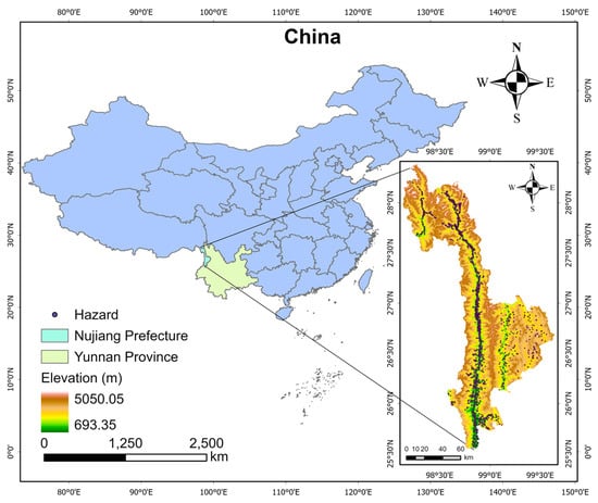
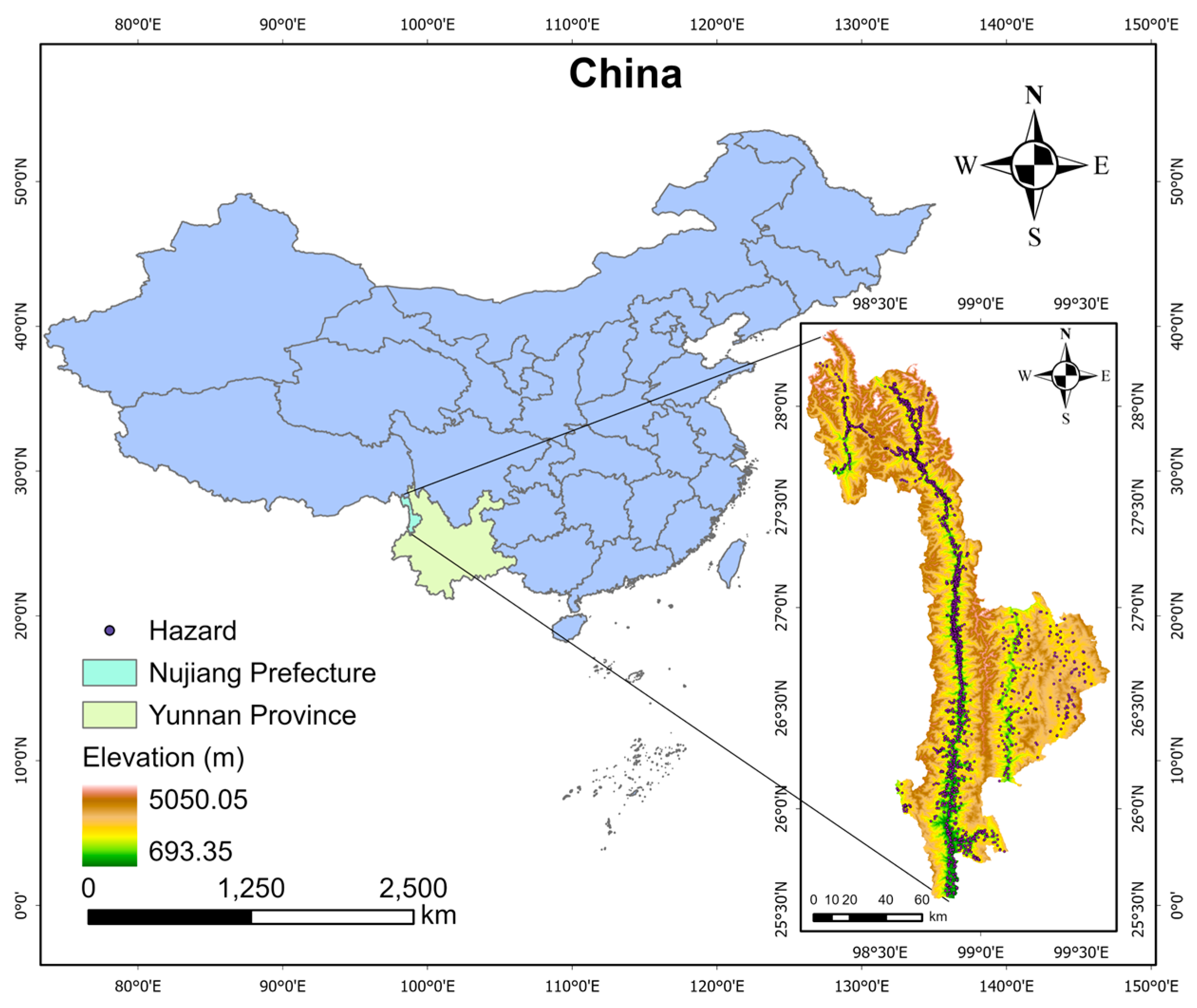
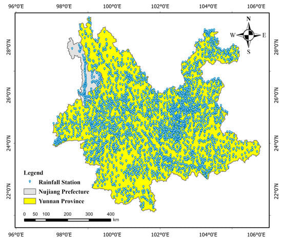
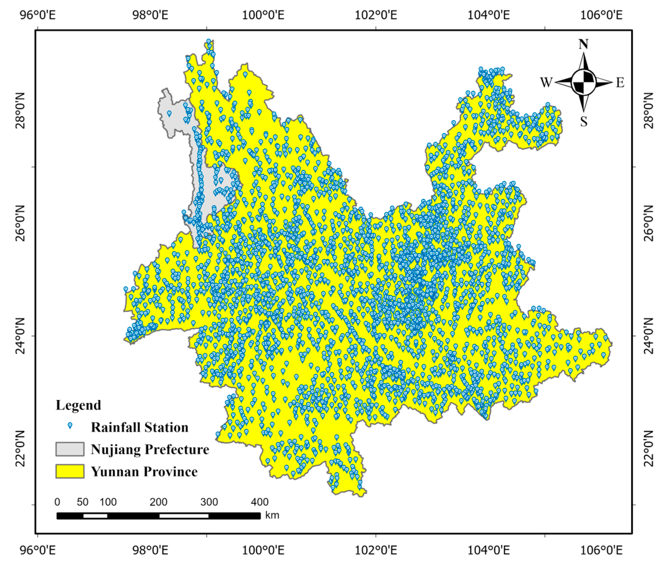
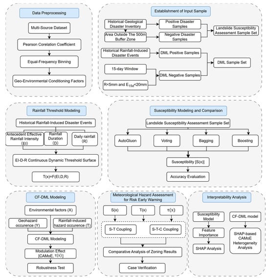
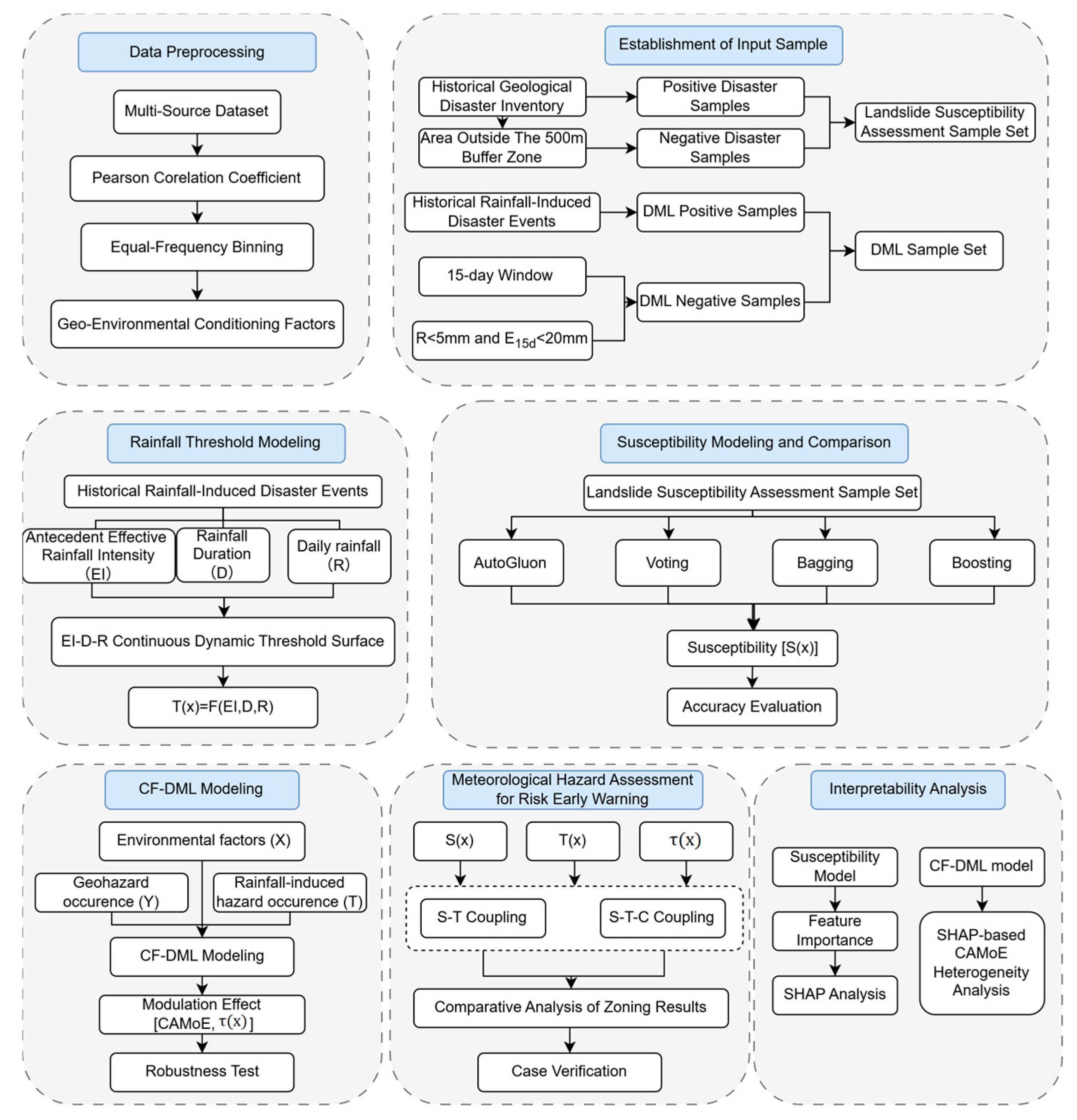
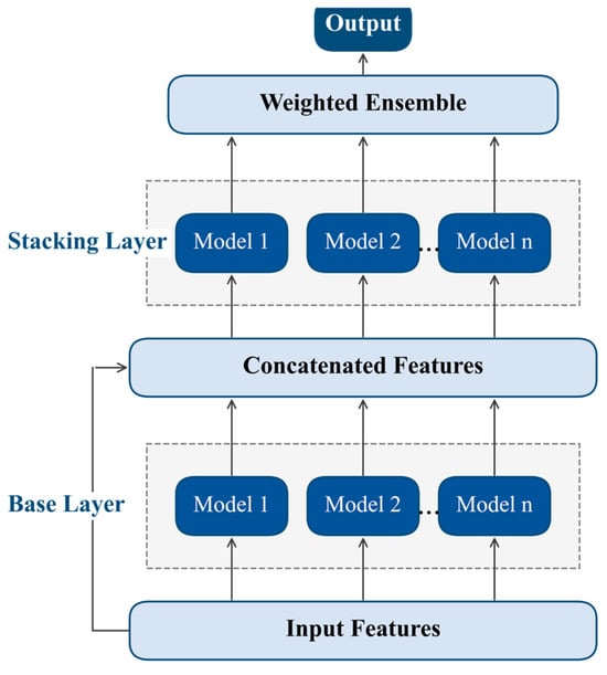
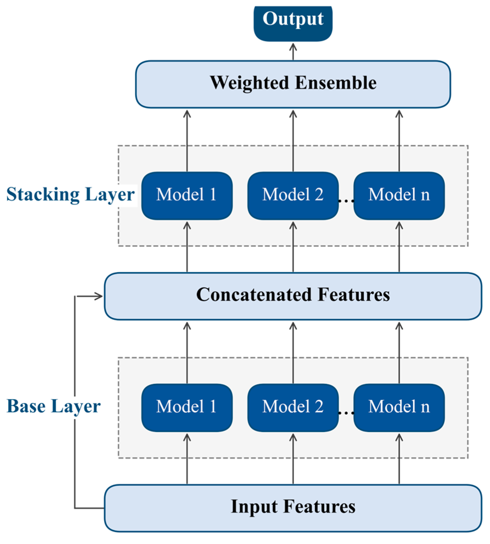
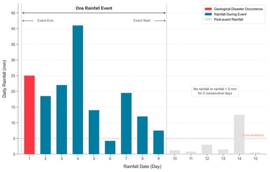
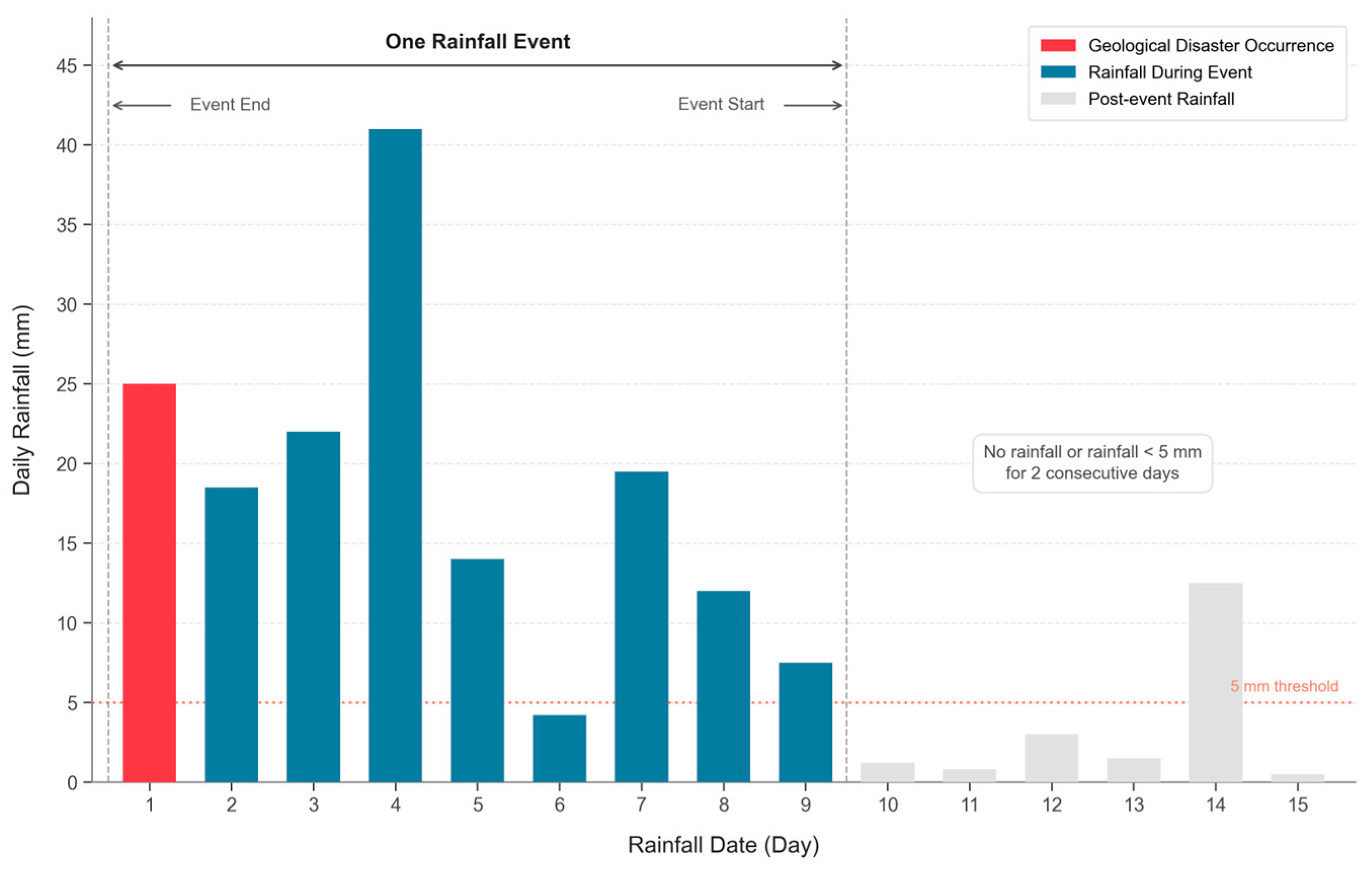
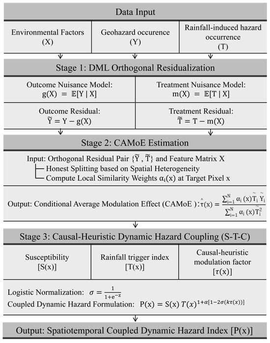
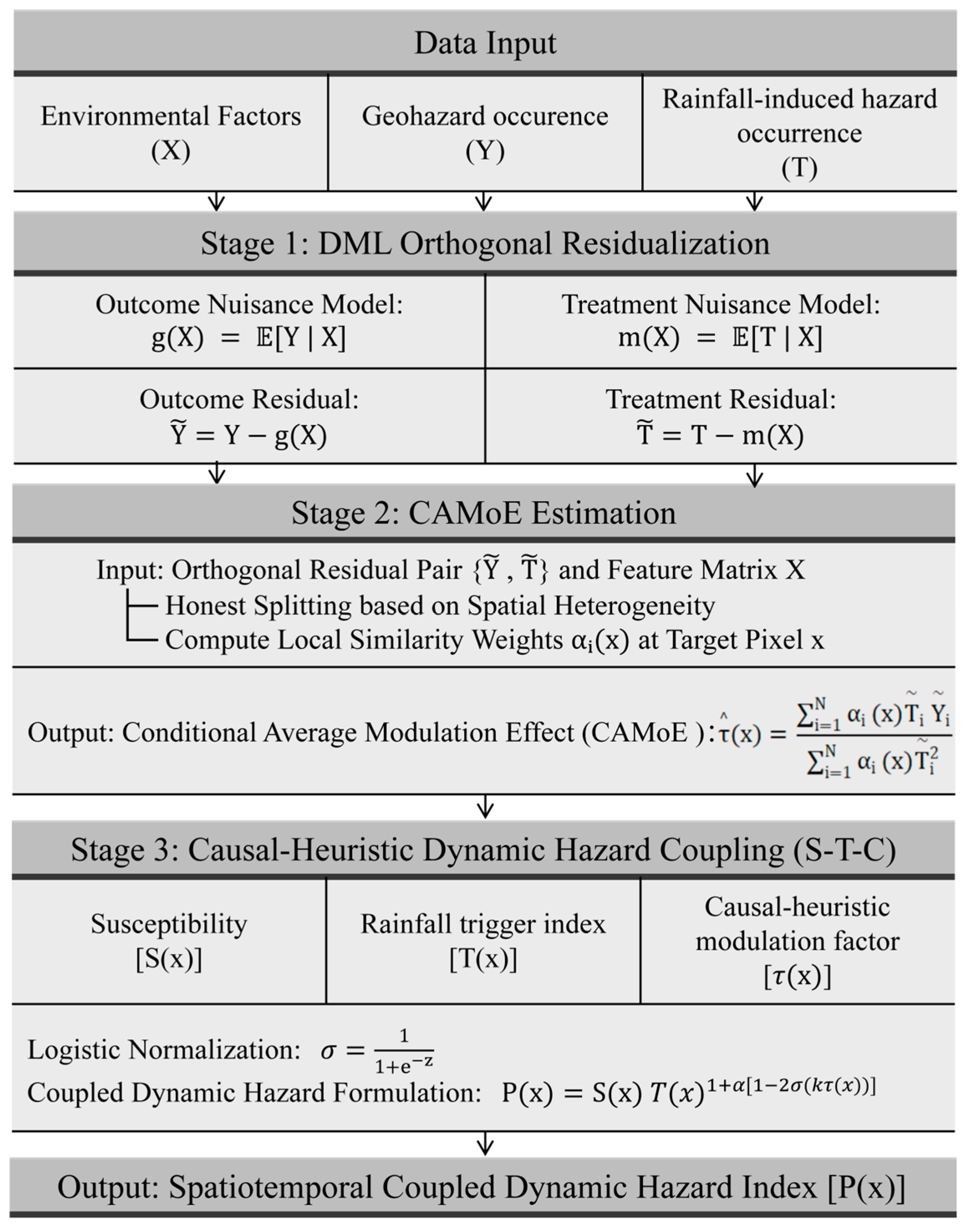
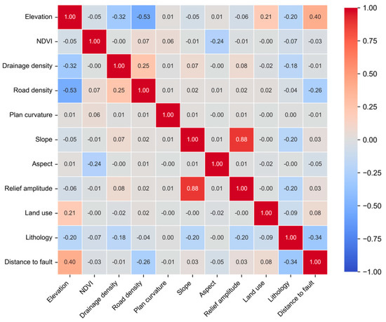
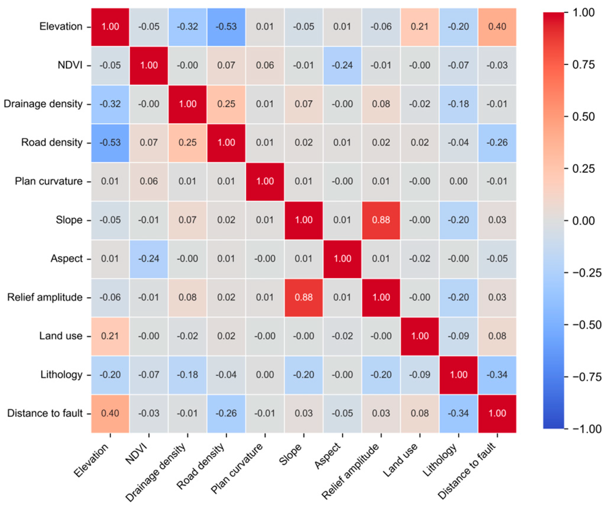
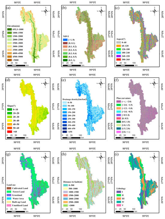
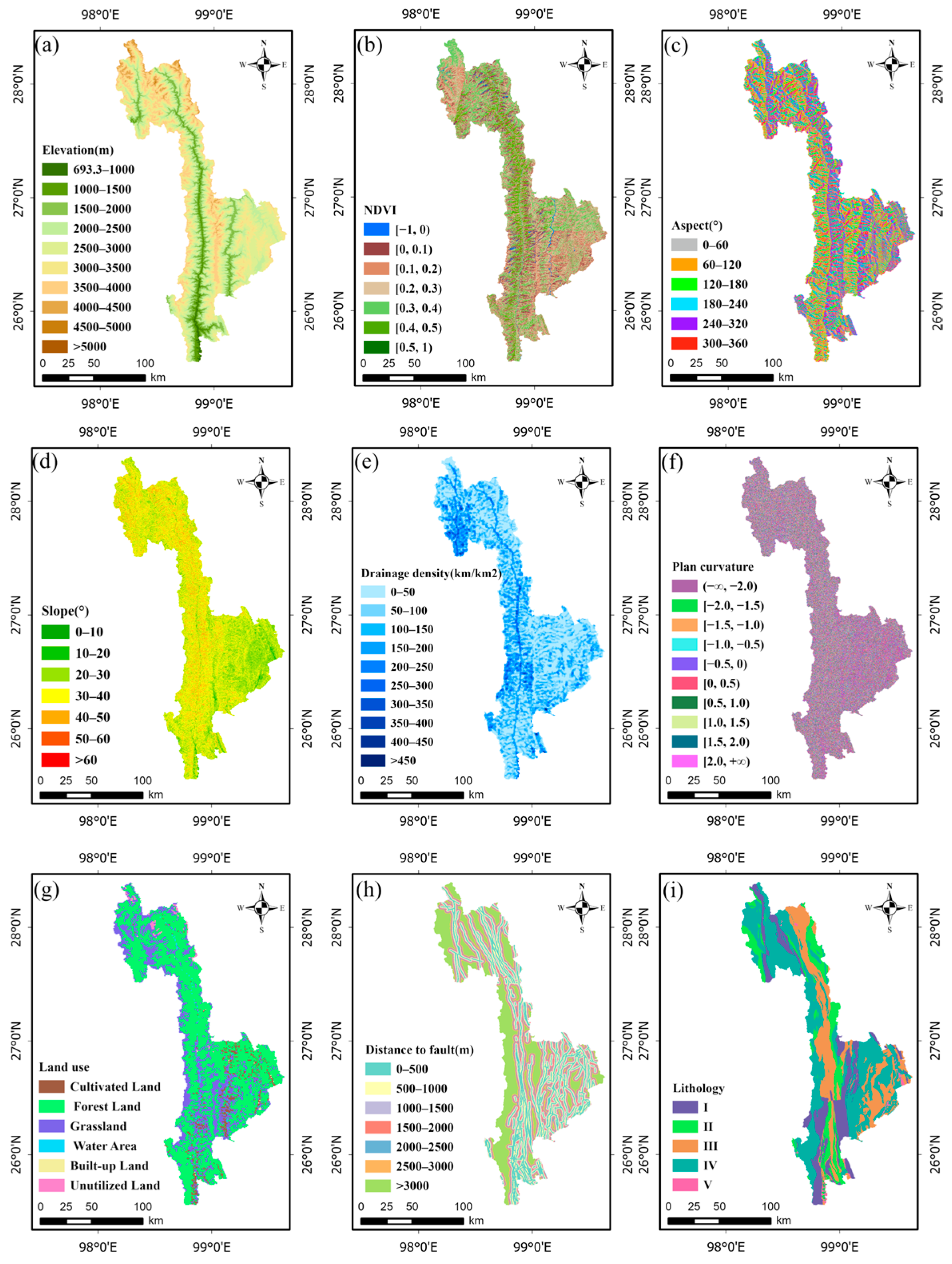
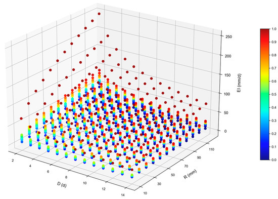
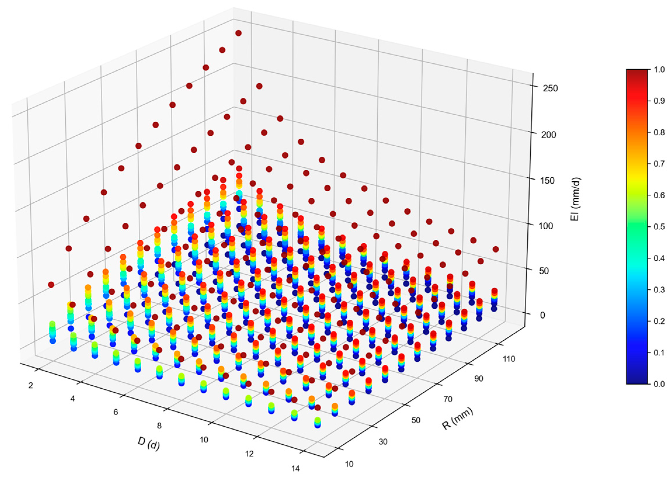
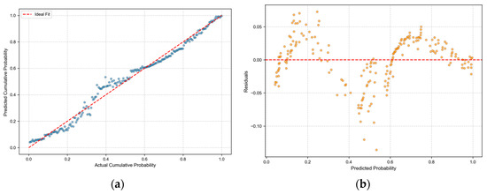
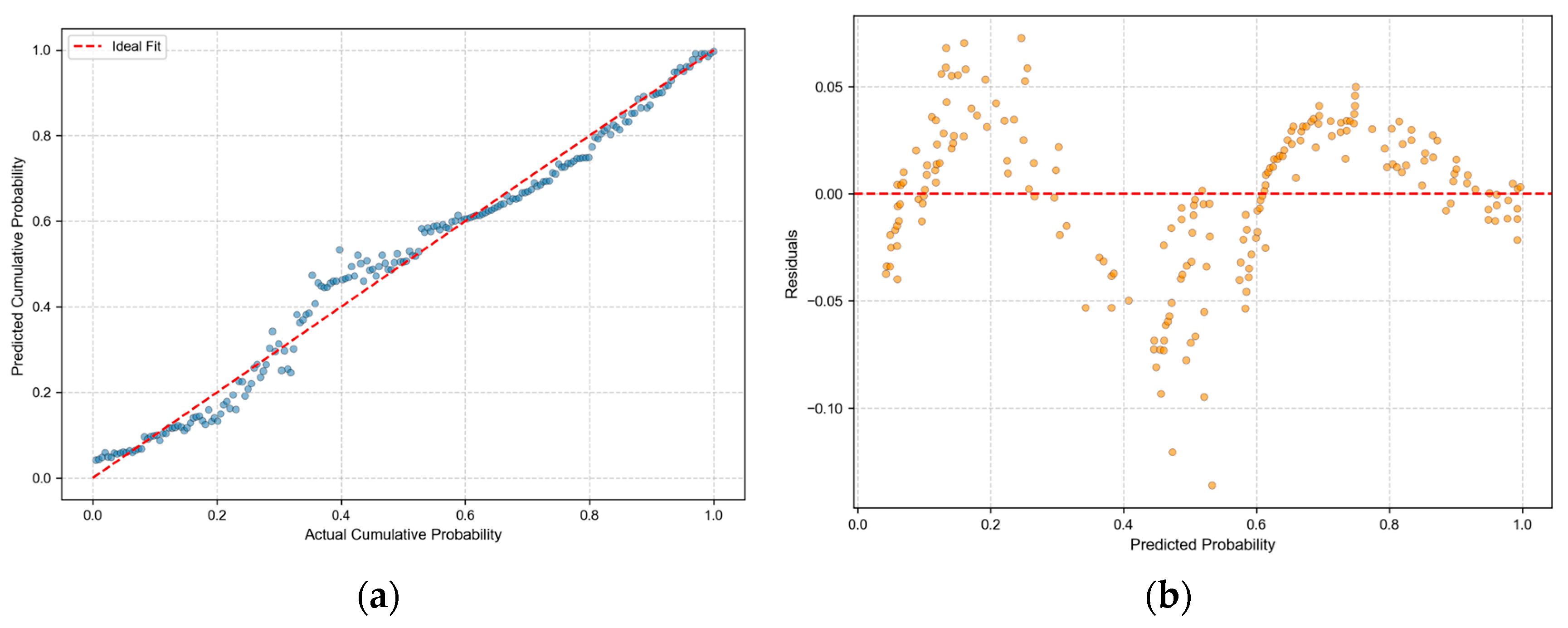
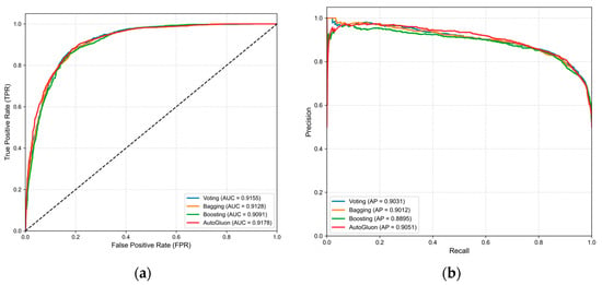
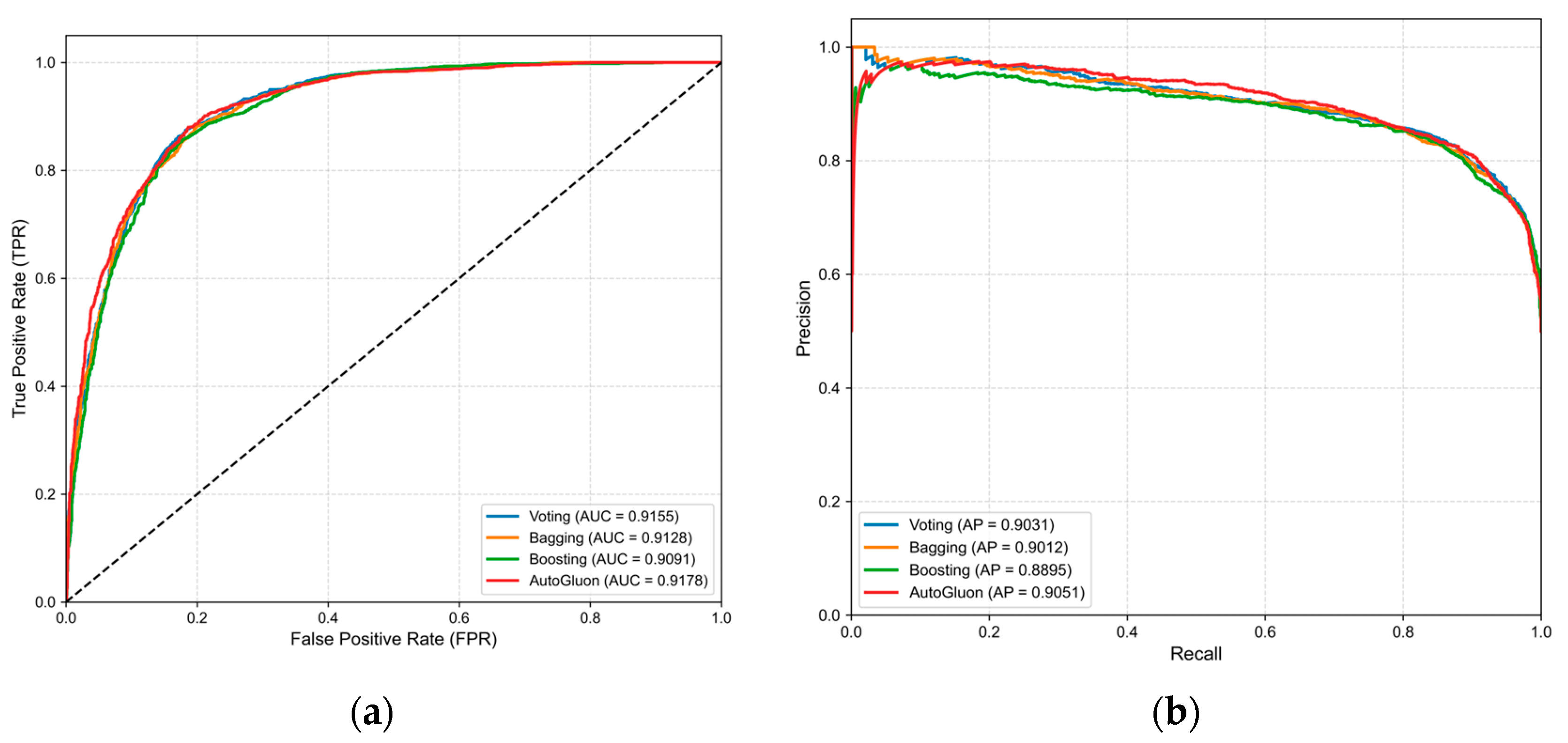
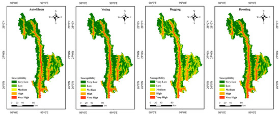
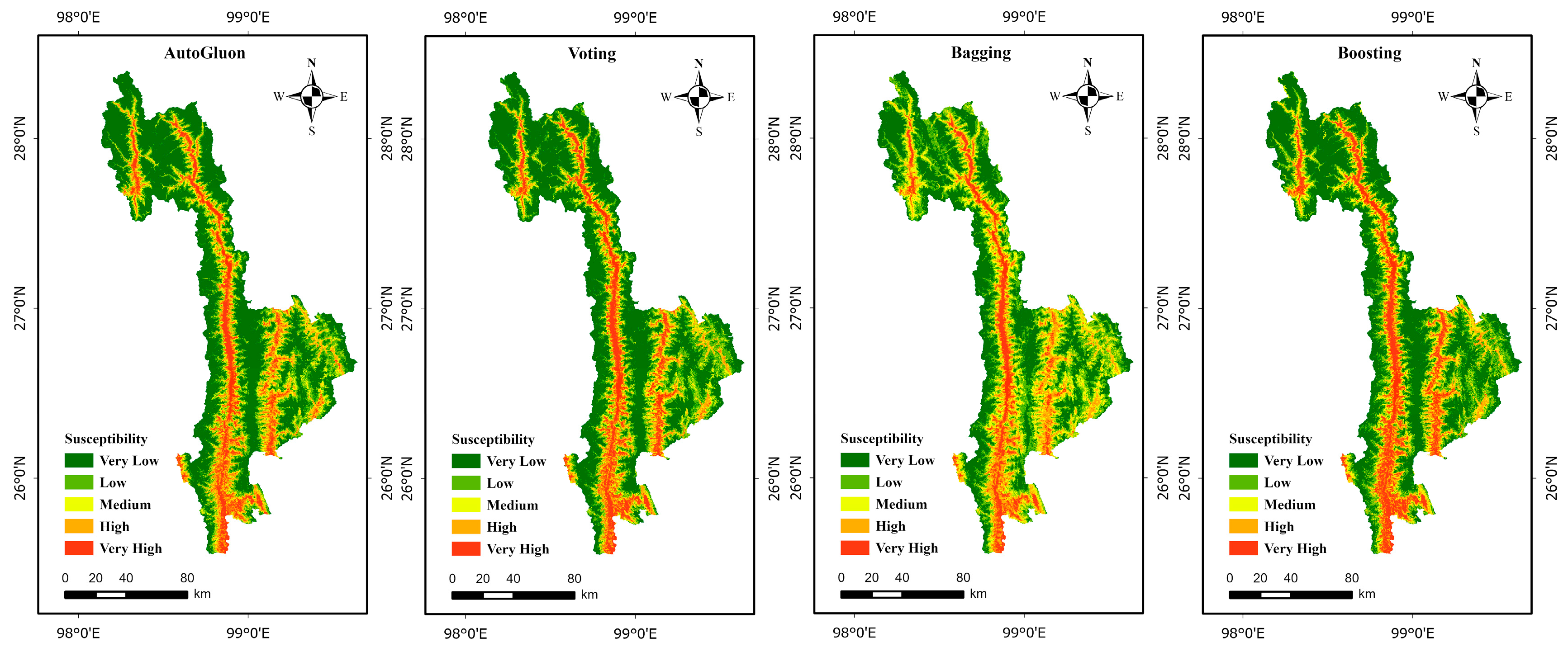
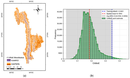
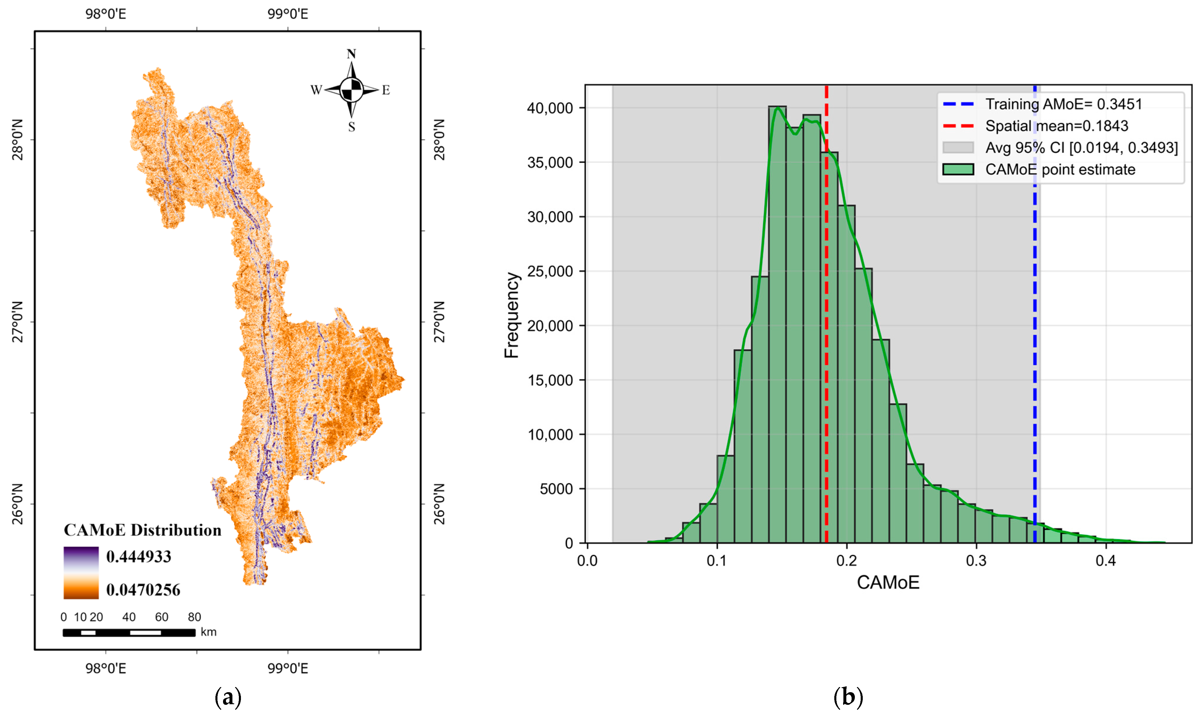
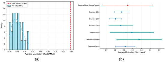
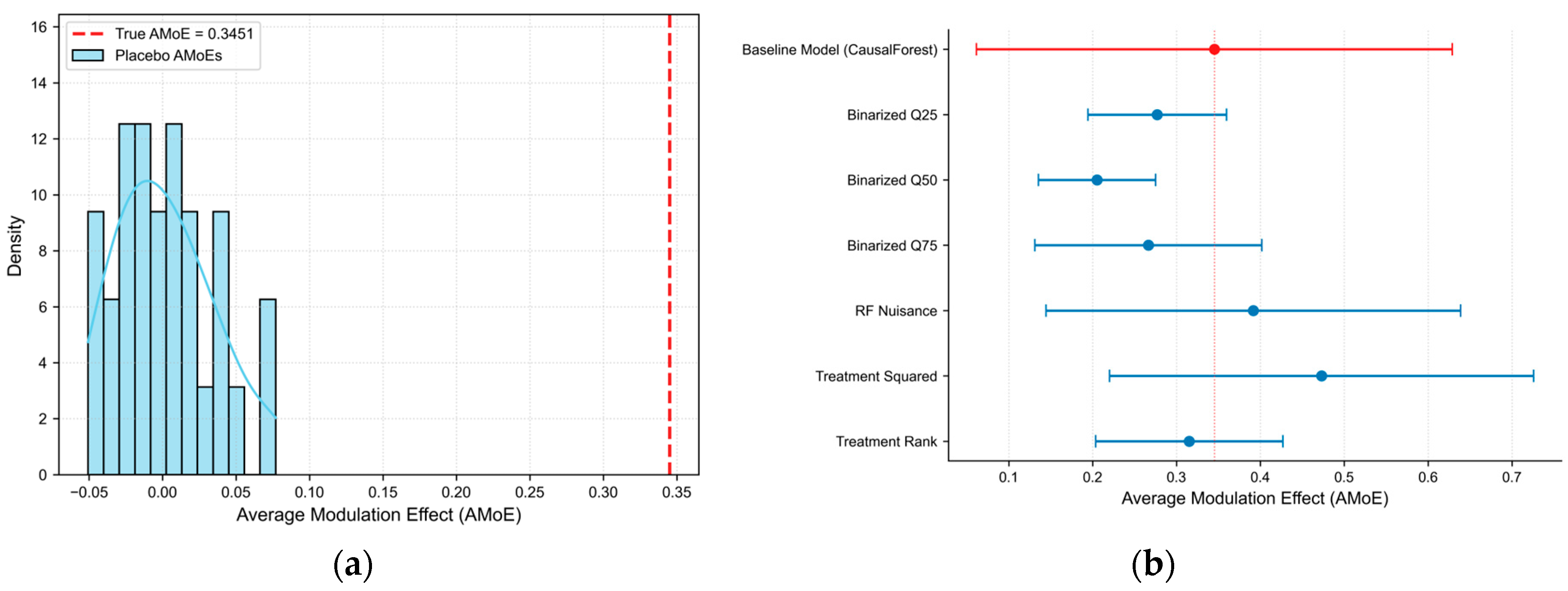
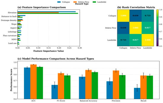
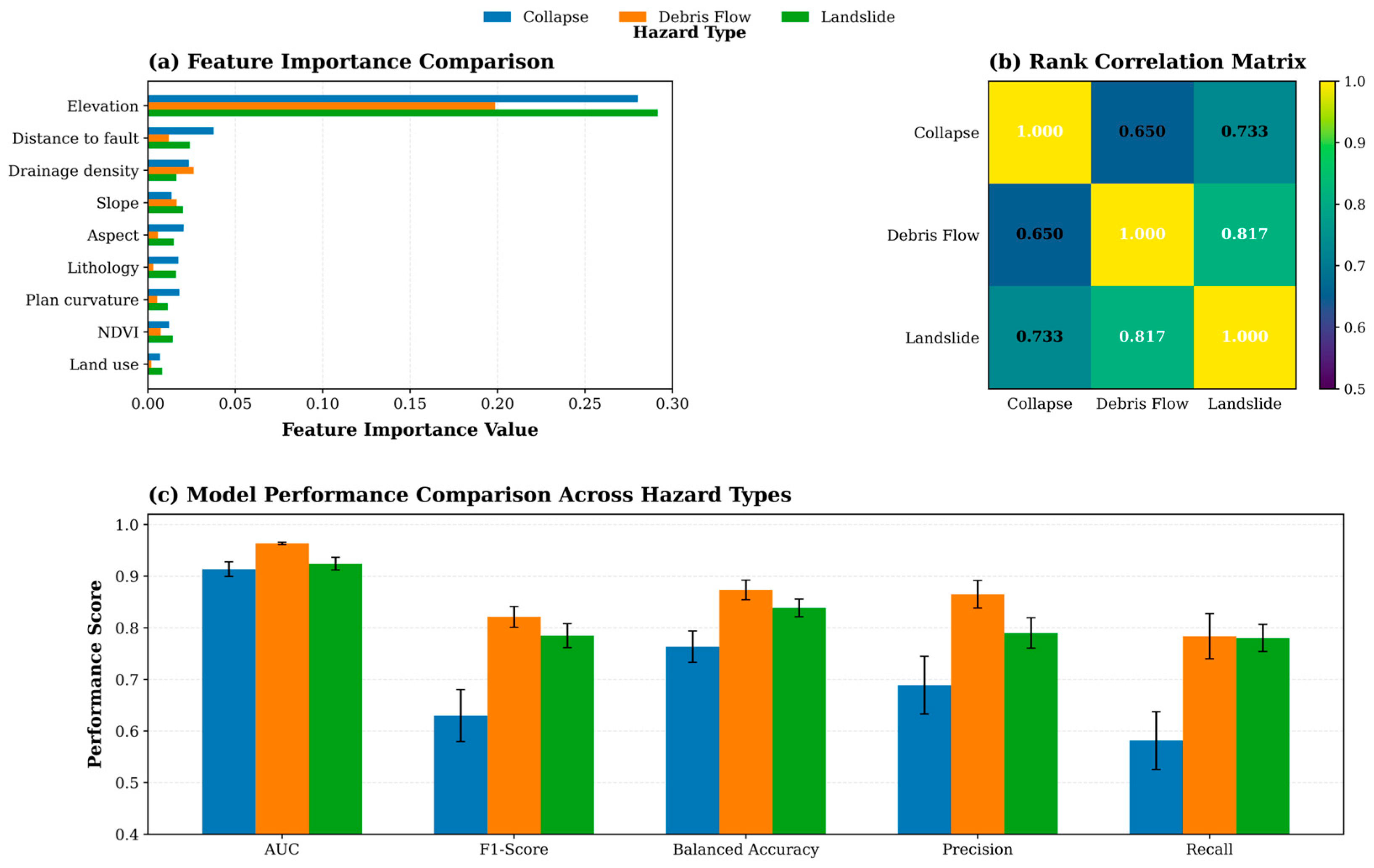
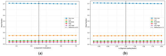
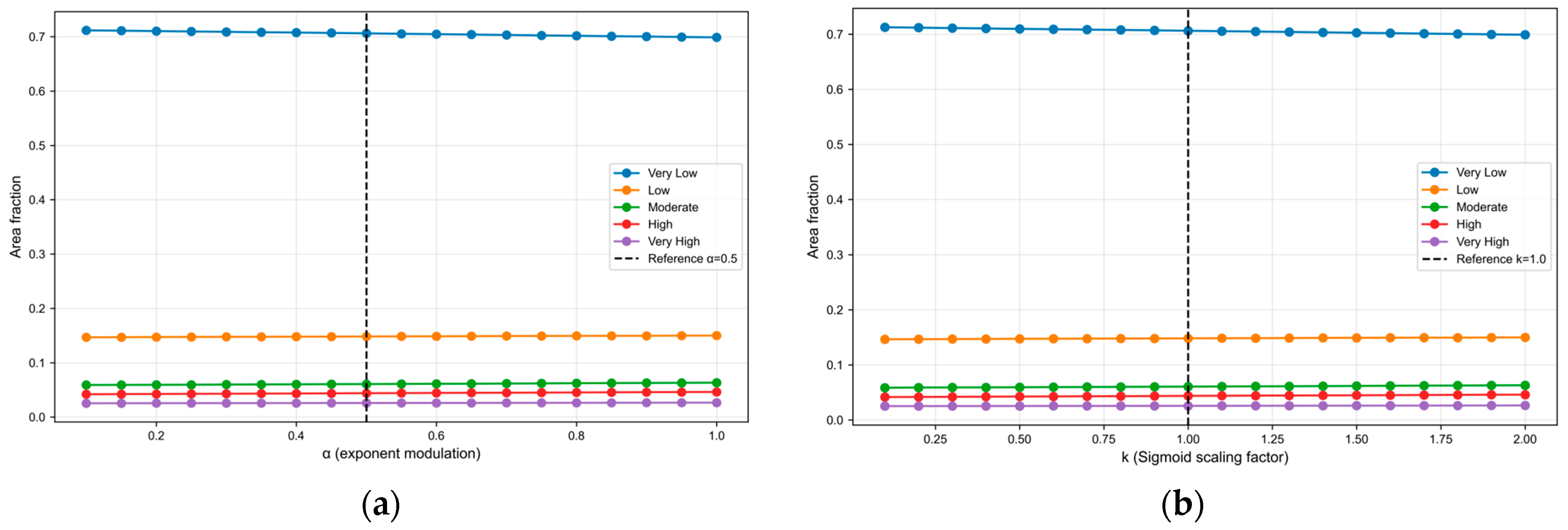
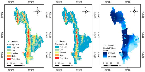
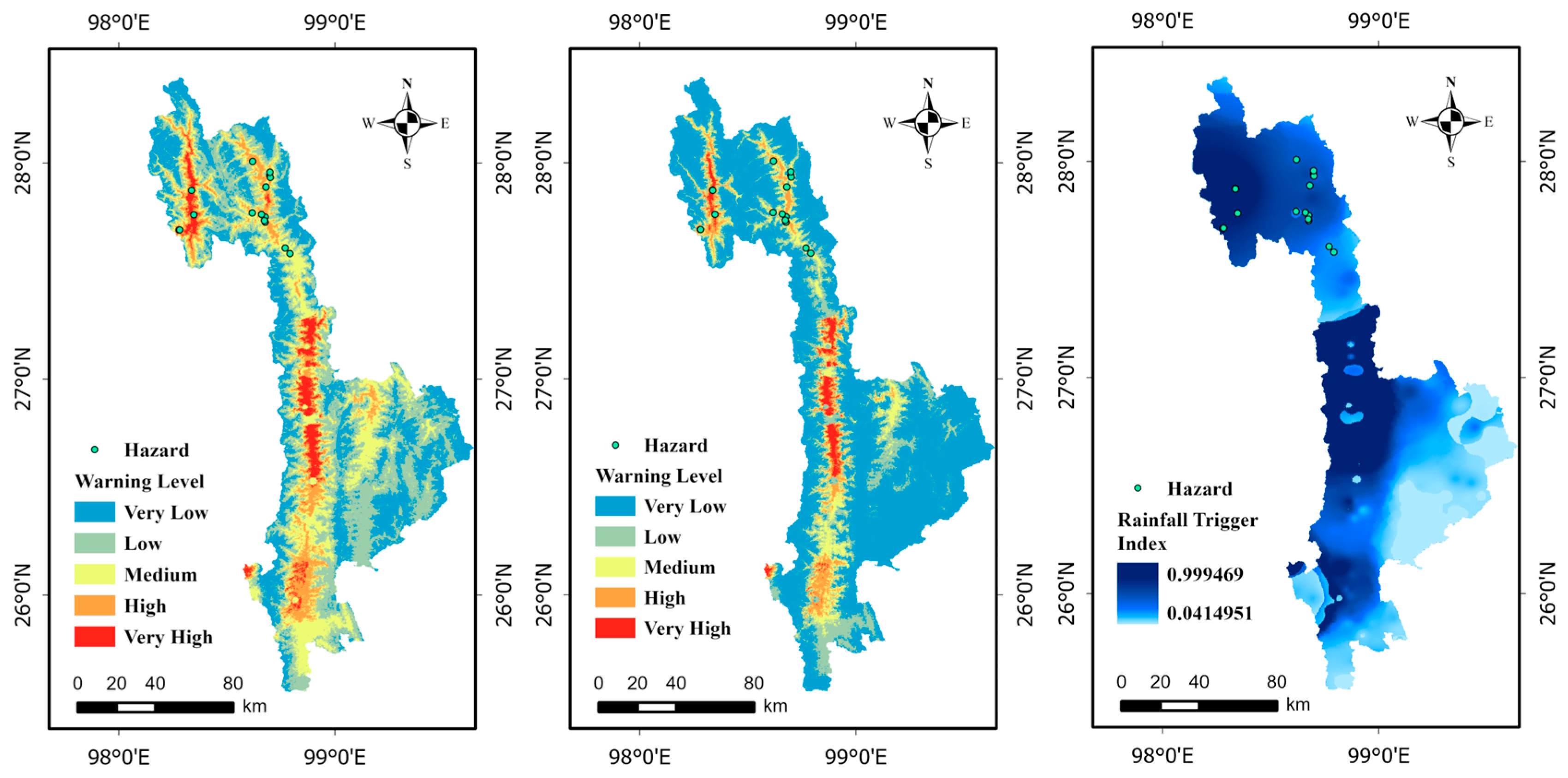
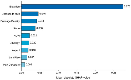
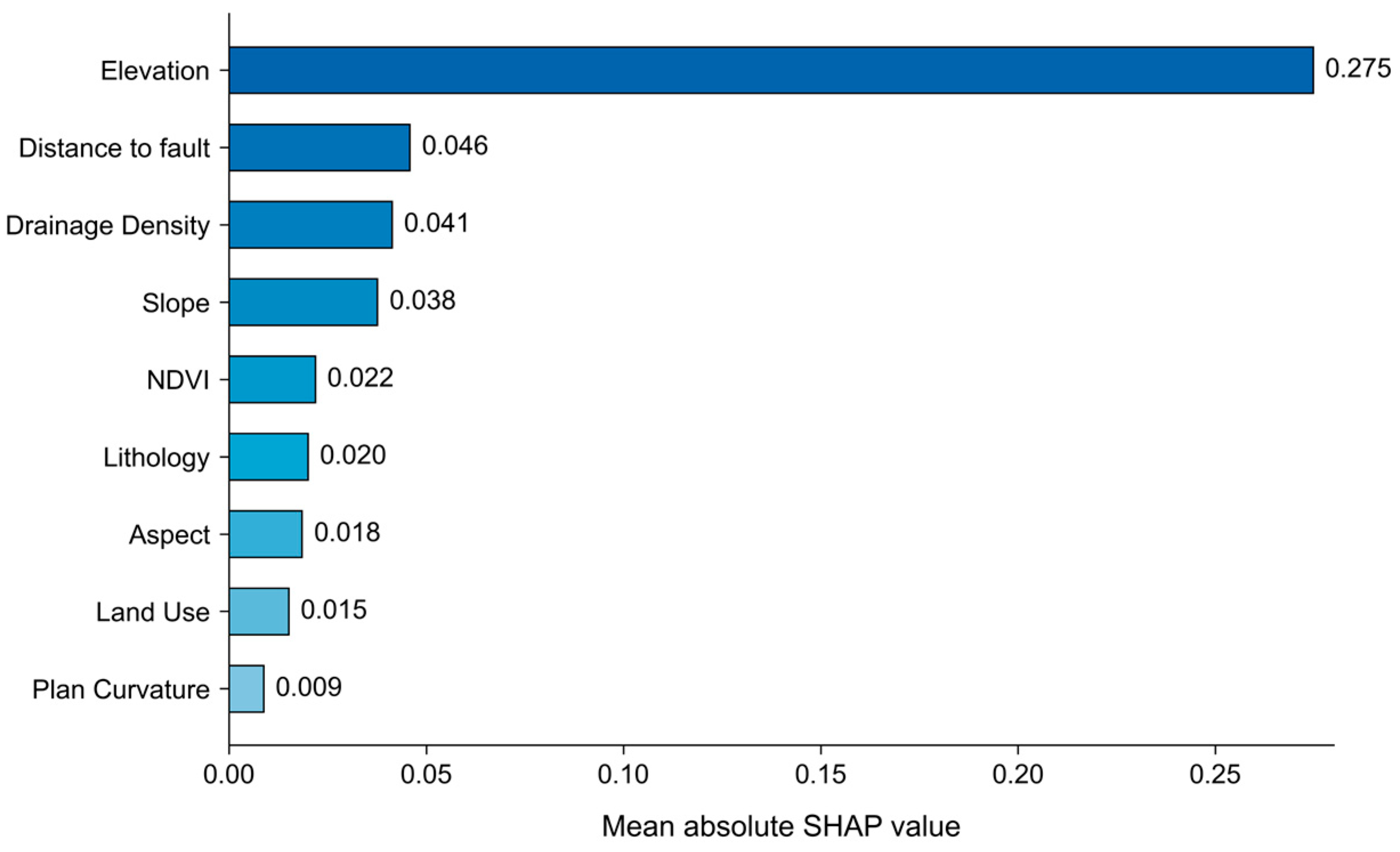
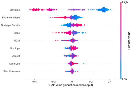
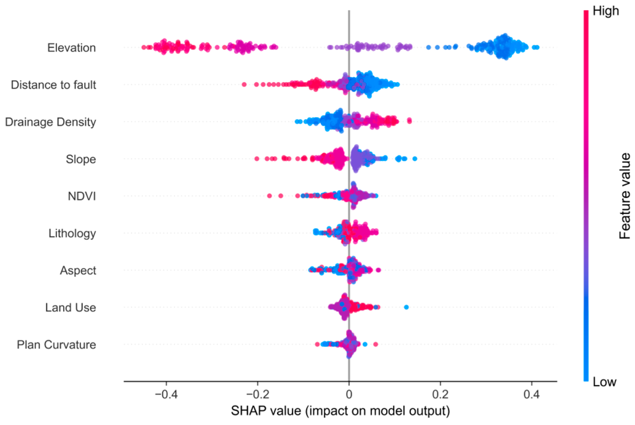
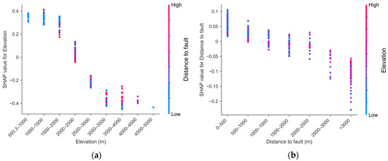
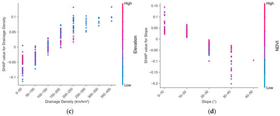
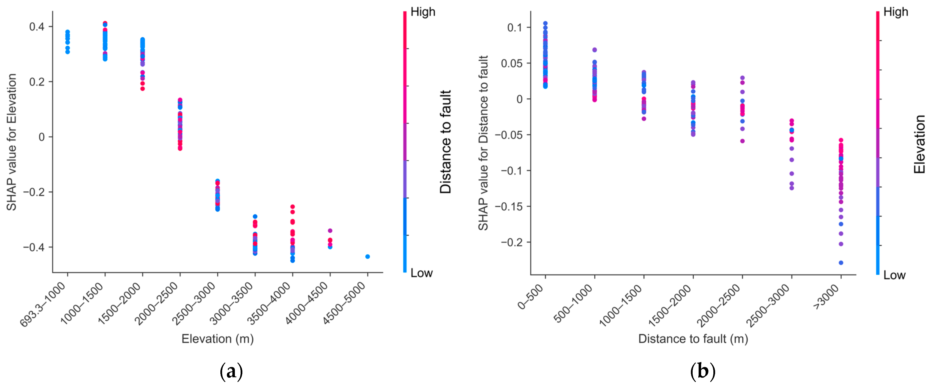
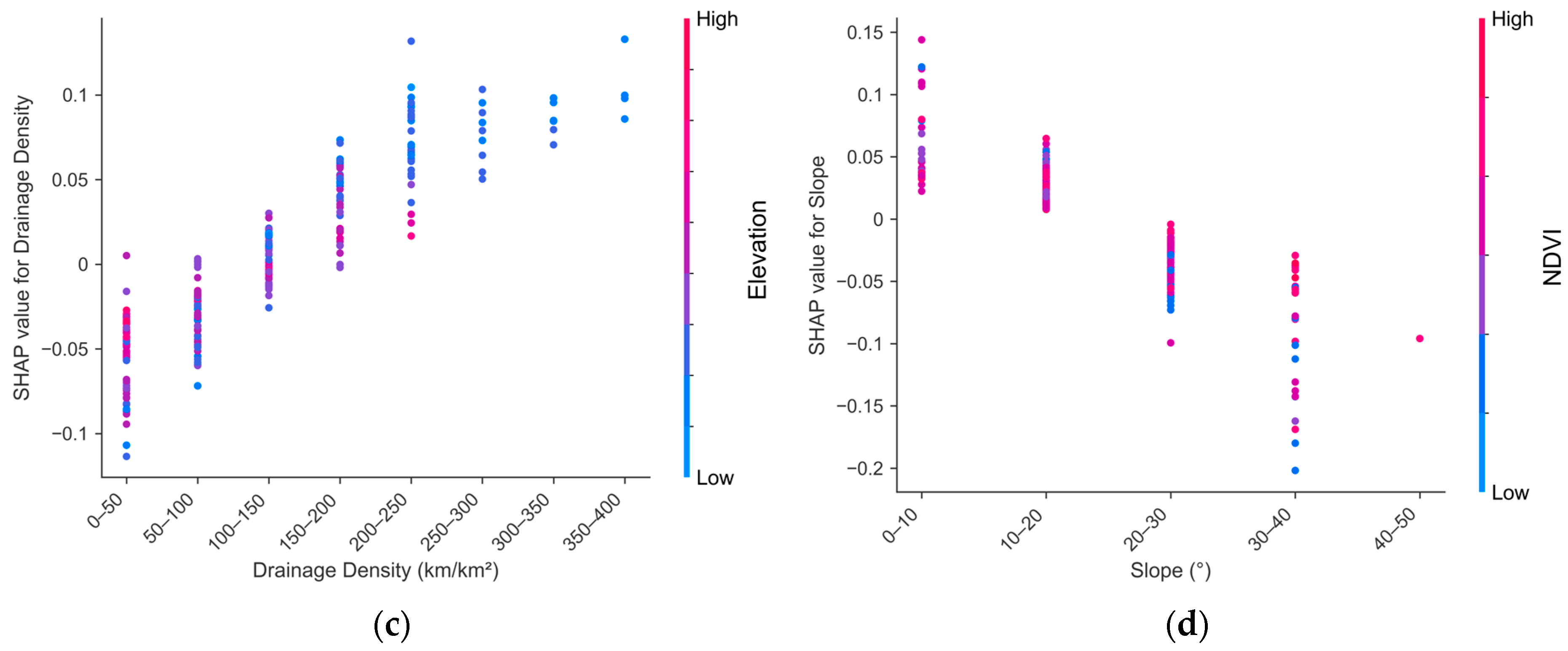
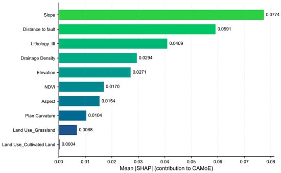
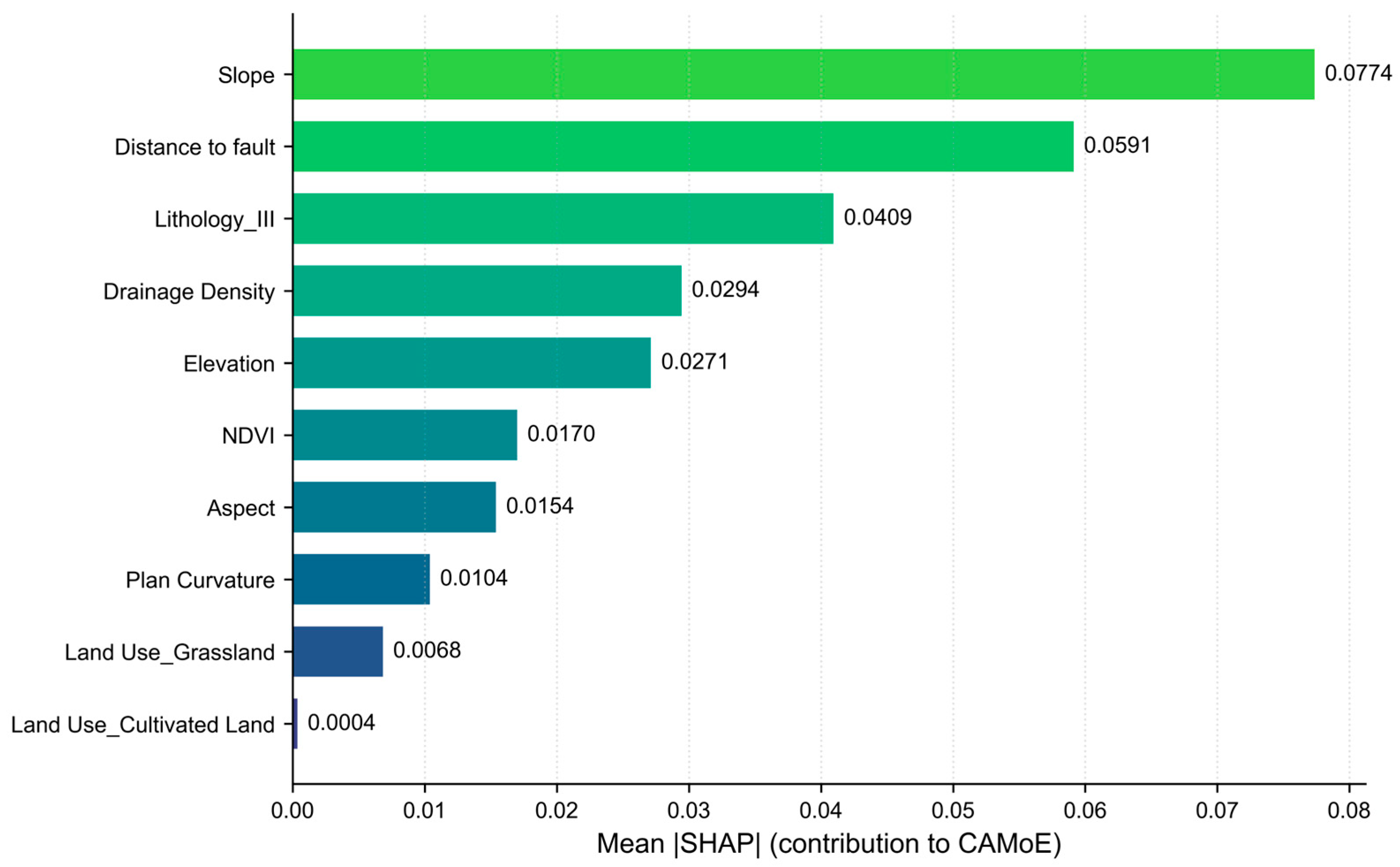

Disclaimer/Publisher’s Note: The statements, opinions and data contained in all publications are solely those of the individual author(s) and contributor(s) and not of MDPI and/or the editor(s). MDPI and/or the editor(s) disclaim responsibility for any injury to people or property resulting from any ideas, methods, instructions or products referred to in the content. |
© 2026 by the authors. Licensee MDPI, Basel, Switzerland. This article is an open access article distributed under the terms and conditions of the Creative Commons Attribution (CC BY) license.