Spatial Leakage in Classifying NASA FIRMS Thermal Anomalies as Wildfire Incidents: A Leakage-Controlled Evaluation of Radiometric, Temporal, and Spatiotemporal Features

Abstract

NASA’s Fire Information for Resource Management System (FIRMS) provides near-real-time thermal anomaly detections from VIIRS, but not all detections correspond to wildfire incidents: industrial heat, agricultural burning, and sensor artifacts produce false alarms that contribute to alert fatigue for emergency-management analysts. We study whether contextual machine learning (ML) features improve wildfire-incident classification from FIRMS detections, and—more importantly—whether reported gains survive leakage-controlled evaluation. We construct a labeled dataset by matching 521,395 VIIRS SNPP detections across CONUS in 2024 to 3766 NIFC 2024 wildfire perimeters, yielding 131,771 (25.3%) wildfire-matched and 389,624 candidate non-wildfire detections spanning 1067 distinct wildfire incidents. We benchmark five operational baselines and six classifiers under four validation regimes (random, event-aware, 5° spatial-block, and temporal holdout) with and without raw geographic coordinates. A naive random split inflates LightGBM to F1 = 0.985, but a leakage-controlled event-aware split reduces it to F1 = 0.767, and a spatial-block holdout to F1 = 0.627. Feature attribution shows geographic coordinates account for 88.9% of model gain—the summed share of LightGBM’s total split-gain attributed to the three coordinate features within the full-feature model; removing coordinates improves spatial-block generalization from F1 = 0.627 to 0.818, demonstrating that raw coordinates drive memorization of where 2024 fires occurred rather than transferable discrimination. We further show that spatiotemporal clustering must be causal: a model using full-partition clustering appears strong (F1 = 0.908) but leaks future detections, whereas a properly causal trailing-window version ties plain LightGBM in-distribution (F1 = 0.762). Combining causal clustering with no raw coordinates is the most robust configuration under spatial transfer (spatial-block F1 = 0.868 vs. 0.627 for the coordinate model). Bootstrap 95% confidence intervals show these gaps far exceed statistical uncertainty, and sensitivity analyses show the conclusions are robust to the spatial-block size and to the clustering-window choice. Under natural class prevalence (14%), precision falls to 0.69, and results are sensitive to the labeling buffer. All ML models nonetheless far exceed FIRMS high-confidence thresholding (F1 = 0.128). We argue that spatial leakage—not raw accuracy—is the central methodological issue for FIRMS wildfire-incident classification, and recommend coordinate-free, causal spatiotemporal-clustering features evaluated under spatial holdout. The system is intended as an analyst-prioritization decision-support layer, not autonomous incident confirmation.

1. Introduction

Wildfires are among the most destructive and rapidly evolving natural hazards, causing loss of life, community destruction, and continental-scale air-quality degradation [1,2]. NASA’s FIRMS delivers active fire detections from MODIS and VIIRS instruments within approximately three hours of satellite overpass [3,4], making it a critical data source for emergency-management platforms worldwide.

However, FIRMS detects thermal anomalies—not confirmed wildfire incidents. Known non-wildfire sources include industrial heat (power plants, refineries), agricultural burning [5], gas flares [6], volcanic activity, and sensor artifacts. These false positives contribute to alert fatigue and the “cry-wolf” effect, in which repeated false alarms erode responder trust and degrade decision-making [7]. Conversely, dismissing uncertain detections risks missing genuine wildfires—particularly small or early-stage fires—with asymmetric consequences: a missed wildfire can grow rapidly, while a false alarm costs only analyst time.

Existing FIRMS products provide confidence classifications from radiometric context alone, without integrating temporal or geospatial information. A natural hypothesis is that contextual ML can improve discrimination. Prior internal drafts of this work reported F1 above 0.98 for tree-based models—a result that, on inspection, is an artifact of spatial and event leakage under random train/test splitting. This paper therefore asks two questions: (i) Can contextual ML features improve wildfire-incident classification from FIRMS thermal anomalies over operational baselines? (ii) Do those gains survive leakage-controlled validation, or are they driven by memorization of known fire locations?

We state the feature scope explicitly at the outset to avoid confusion: the experiments reported in this paper use only VIIRS radiometric attributes, derived temporal features, geographic coordinates, and causal spatiotemporal-density features. Weather, land-cover, and terrain variables are not included in any reported experiment; they are part of the intended multi-source design and are discussed only as future work (Section 5.10 and Section 5.11; Appendix A).

Contributions

• We formulate FIRMS wildfire-incident classification as a supervised ML task distinct from pixel-level thermal anomaly detection, and build an event-linked labeled dataset (521,395 detections, 1067 incidents).
• We show that naive random splitting overstates F1 by roughly 0.22 absolute (0.985 vs. 0.767) due to spatial/event leakage, and quantify this across four validation regimes, with bootstrap confidence intervals quantifying the statistical uncertainty of all headline comparisons.
• We perform a geographic feature-sensitivity analysis showing that raw geographic coordinates account for 88.9% of gain (the summed split-gain share of the three coordinate features; the calculation is defined in Section 4.8) yet harm spatial-block generalization, the hallmark of memorization; a block-size sensitivity analysis (2.5°, 5°, 10°) shows this conclusion is not an artifact of the block size.
• We show that spatiotemporal clustering must be causal (trailing-window): full-partition clustering leaks future detections, and only the causal, coordinate-free variant is the most robust under spatial transfer, a result that is insensitive to halving or doubling the 6 h/24 h clustering windows.
• We report calibration, natural-prevalence performance, error modes, and qualitative failures relevant to emergency-management deployment.

2. Related Work

2.1. Satellite Active Fire Detection and False Positives

The MODIS Collection 6 active fire product uses contextual brightness temperature thresholding at 1 km resolution [3,8]; VIIRS provides 375 m resolution via the I-band algorithm [4]. Both instruments prioritize sensitivity over specificity, yielding commission error rates of 10–30% [3]. Elvidge et al. [6] documented gas-flare false positives, Artés et al. [9] cataloged non-wildfire active fire detections globally, and McCarty et al. [5] characterized agricultural burning that is thermally similar to wildfire. These studies motivate treating “is this detection a wildfire incident?” as a classification problem layered on top of detection.

2.2. Wildfire Event Extraction and ML

Andela et al. [10] extract individual fire events from active fire time series, providing an event abstraction that we mirror with NIFC incident grouping. Jain et al. [11] survey ML in wildfire science. Grinsztajn et al. [12] show tree-based methods outperform deep learning on heterogeneous tabular data; Random Forest [13], XGBoost [14], and LightGBM [15] are standard for tabular remote-sensing classification. ML studies of wildfire occurrence and susceptibility frequently report very high discrimination (ROC-AUC above 0.9) under random cross-validation, e.g., Tonini et al. [16] for susceptibility mapping in Liguria; Section 5 discusses how such figures relate to the leakage-controlled estimates reported here.

2.3. Spatial Leakage and Spatial Cross-Validation

A growing literature warns that random cross-validation is over-optimistic for spatially autocorrelated data, because nearby train/test samples are not independent [17,18]. Meyer et al. [19] show specifically that including spatial coordinates (or strongly location-correlated predictors) inflates apparent accuracy while degrading transfer to new regions, and recommend spatial variable selection and spatial-block validation. Kattenborn et al. [20] demonstrate the same inflation for deep models when training and validation samples are spatially autocorrelated. Our findings are a direct instance of this phenomenon in the FIRMS wildfire-classification setting, and we adopt event-aware and spatial-block holdouts as the appropriate evaluation protocol.

3. Materials and Methods

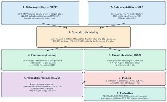
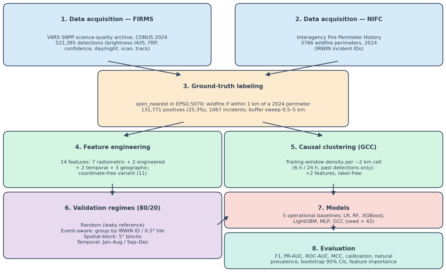
Figure 1 summarizes the end-to-end methodology: data acquisition from FIRMS and NIFC, ground-truth labeling, feature engineering (including the causal-clustering variant), the four validation regimes, model training, and evaluation. The following subsections describe each stage.

Figure 1. Overview of the study workflow: data acquisition (FIRMS VIIRS SNPP detections and NIFC wildfire perimeters), ground-truth labeling with a 1 km buffer, feature engineering (14 features; 11-feature coordinate-free variant; +2 causal-clustering features for the GCC), four validation regimes, model training, and evaluation.

3.1. Data Sources

Table 1 summarizes the data sources used. We emphasize at the outset that the empirical evaluation in this paper uses only VIIRS radiometric attributes, derived temporal features, and geographic coordinates: weather, land-cover, and terrain layers are part of the intended multi-source design but are not integrated in this dataset release, and we deliberately avoid claiming results we did not measure (Section 5.10; Appendix A).

Table 1. Data sources used in this evaluation. Additional layers (weather, land cover, terrain, infrastructure) are part of the planned multi-source design but are not used here; they are listed separately in Appendix A to avoid any implication that they contribute to the reported results.

Source	Variables	Res.	Period	Records
FIRMS VIIRS SNPP	Brightness (I4/I5), FRP, confidence, day/night, scan/track	375 m	2024	521,395
NIFC Perimeters	Fire perimeters, IRWIN ID, dates, acres, type	Polygon	2020–2024	18,484

3.1.1. FIRMS VIIRS Detections

We obtain VIIRS SNPP science-quality archive data from NASA FIRMS for CONUS for calendar year 2024 via the FIRMS Area API: 521,395 detections. Each detection includes latitude, longitude, brightness temperature (Bands I4/I5), fire radiative power (FRP, MW), confidence class (low/nominal/high), day/night flag, scan angle, track, satellite, instrument, and acquisition datetime.

3.1.2. Wildfire Ground Truth

We obtain wildfire perimeters from the NIFC Interagency Fire Perimeter History service: 18,484 perimeters for 2020–2024 covering 34.9 million acres. Each record includes incident name, IRWIN ID, current-perimeter date, GIS acres, fire-type category, and agency. We filter to records categorized as wildfire (final or daily fire perimeter) for 2024, yielding 3766 wildfire perimeters. IRWIN ID provides the incident grouping used for event-aware splitting.

3.2. Labeling Methodology

3.2.1. Task and Positive Labels

Given a FIRMS detection, we classify it as wildfire incident ($y=1$) or non-wildfire thermal anomaly ($y=0$). A detection is labeled $y=1$ if it falls within a spatial buffer $d_s=1000$ m of a 2024 wildfire perimeter (computed with sjoin_nearest in EPSG:5070 projected coordinates). When a detection matches multiple perimeters, the nearest is used, and its IRWIN ID is recorded as the detection’s incident group. This yields 131,771 positives (25.3%) across 1067 distinct incidents.

Choice of the 1 km Buffer

The 1 km buffer is derived from the positional error budget of the detection-to-perimeter match, not tuned for classifier performance. VIIRS I-band pixels are 375 m at nadir but grow to roughly 750 m across-scan toward the swath edge [4], and the reported coordinates are pixel centers, so the true hot spot can lie several hundred meters from the reported point. NIFC perimeters add their own digitization and temporal-lag error, since a mapped perimeter may trail the actual fire edge by hours. A 1 km tolerance therefore covers approximately two pixel widths of combined positional uncertainty while remaining small relative to the typical separation between distinct incidents. Because this parameter directly shapes the generated ground truth, we treat it as a first-class source of uncertainty rather than a fixed constant: Section 4.11 reports a full sensitivity sweep over $\{0.5,1,2,5\}$ km and all headline metrics should be interpreted jointly with that sweep. Notably, the coordinate-free clustering model is far more stable across buffers than the coordinate model, so the paper’s methodological conclusions do not hinge on the specific buffer value.

3.2.2. Candidate Negatives and Their Composition

A detection unmatched at $d_s$ is treated as a candidate negative (389,624; 74.7%). We use “candidate” because unmatched detections may include unreported small fires. Because the difficulty of the task depends on what the negatives are, Table 2 reports their composition by source. Notably, only 40.3% are spatially isolated (>50 km from any 2024 wildfire); the remaining 59.7% lie within 50 km of a wildfire or recur persistently, making them non-trivial negatives.

Table 2. Candidate-negative composition ($N=\mathrm{389,624}$). Categories are mutually exclusive in the order listed.

Source	Count	%
Persistent hot source (>30 d span, <100 m cell)	91,046	23.4
Spatially isolated (>50 km from any 2024 wildfire)	157,064	40.3
Other unmatched (<50 km, non-persistent)	141,514	36.3
Total candidate negatives	389,624	100.0

3.2.3. Class Balance and Sampling

The raw labeled stream is imbalanced (25.3% positive). For model comparison we balance-sample up to 40,000 detections per class within each split’s groups (the training balanced set is 80,000 detections), so that F1 and the confusion matrix are not dominated by prevalence. We additionally report a natural-prevalence evaluation (Section 4.10) on all detections in the held-out event groups (98,071 detections, 14.0% positive), because precision and analyst workload are prevalence-dependent.

3.3. Feature Engineering

We construct a 14-dimensional feature vector from four groups available locally (Table 3). A coordinate-free variant drops the three geographic features (11 features).

Table 3. Feature groups used in this evaluation (14 features). The GCC variant appends two causal trailing-window cluster features.

Group	Features
Satellite (7)	bright_ti4, bright_ti5, FRP, confidence, day/night, scan, track
Engineered (2)	$\Delta T=T_{I4}-T_{I5}$, $log(1+\mathrm{FRP})$
Temporal (2)	month, hour
Geographic (3)	latitude, longitude, $\left|\mathrm{latitude}\right|$
Cluster (GCC, +2)	dens_6h, dens_24h (causal trailing-window density)

3.3.1. Causal Spatiotemporal Clustering

The GCC variant appends two causal density features: the count of detections in the same ∼2 km cell within the trailing 6 h and 24 h, computed over the time-ordered stream using only detections at or before each detection’s acquisition time (Section 3.4). The intuition is that genuine wildfires generate temporally persistent, spatially dense detection clusters, whereas isolated industrial or agricultural sources do not; density is therefore a candidate generalizable discriminator that does not encode absolute location.

3.3.2. Choice of the 6 h and 24 h Windows

The window lengths are anchored to the VIIRS SNPP overpass cadence rather than tuned. SNPP images CONUS approximately twice per day (ascending ∼13:30 and descending ∼01:30 local overpasses, with additional adjacent-swath repeats at high scan angles) [4]. The 6 h window therefore captures persistence within the most recent overpass epoch, while the 24 h window spans one full diurnal cycle containing both a day and a night overpass. To verify that this choice is not load-bearing, Section 4.4 reports a sensitivity analysis that halves (3 h/12 h) and doubles (12 h/48 h) both windows; coordinate-free GCC performance changes by at most 0.008 F1 under either the event-aware or the spatial-block regime.

3.3.3. Note on Weather/Land-Cover Features

The custom fire-weather proxy and land-cover flags described in earlier drafts require ERA5/Open-Meteo and NLCD joins that are not present in this dataset release. We therefore do not report weather, land-cover, or terrain ablations, and we do not claim their effect (Section 5.10). The paper’s title and claims reflect only the radiometric, temporal, and spatiotemporal features actually evaluated.

3.4. Validation Regimes

To separate genuine signal from leakage we evaluate four splitting regimes, each at 80/20:

• Random (stratified): i.i.d. split, stratified by label. This is the (leaky) protocol used in prior drafts.
• Event-aware: GroupShuffleSplit where positives are grouped by NIFC IRWIN incident ID and candidate negatives by 0.5° spatial tile, so no incident or local negative cluster appears in both train and test. This is our primary protocol.
• Spatial-block (5°): Groups are 5° geographic blocks, holding out whole regions to test transfer to unseen geography.
• Temporal: Train on January–August, test on September–December.

Choice of the 5° Block Size

The 5° blocks (∼440–550 km at CONUS latitudes; 65 populated blocks) are chosen so that a held-out block exceeds the spatial extent of any single fire complex and of the strong short-range spatial autocorrelation in fire occurrence, forcing genuine extrapolation to unseen regions rather than interpolation between neighboring cells [18]. To demonstrate that the paper’s central conclusion does not depend on this choice, Section 4.3 repeats the spatial-block experiment with 2.5° (218 blocks) and 10° (20 blocks) and across five random block-to-fold assignments. The smaller 2.5° blocks partially reintroduce spatial leakage (held-out blocks share borders with training blocks), and the larger 10° blocks leave too few groups for stable estimates; 5° balances these failure modes, and at every size the coordinate-free model is at least as accurate on average and markedly more stable than the coordinate model.

For each regime we train with the full 14 features (with lat/lon) and the 11-feature coordinate-free variant (no lat/lon). Causal clustering: The GCC cluster features are the number of detections in the same ∼2 km cell within the trailing 6 h and 24 h, computed over the year-ordered stream so that each detection sees only detections at or before its own acquisition time—never future detections. This avoids the leakage of partition-wide DBSCAN (which can count detections from the entire test period) and matches operational monitoring, where only past overpasses are available. Cluster features use no labels. Preprocessing (scaling for LR/MLP) is fitted on training data only. Model hyperparameters are fixed a priori (seed = 42); we report performance across the full probability-threshold range rather than tuning a single operating point on a separate validation fold.

3.5. Statistical Uncertainty

To support comparisons among models with similar performance, we quantify statistical uncertainty with the nonparametric bootstrap: the held-out test set is resampled with replacement 1000 times, all metrics are recomputed on each resample, and we report percentile 95% confidence intervals (CIs). Because all models are evaluated on the same test detections, model differences are assessed with a paired bootstrap: the F1 difference between two models is recomputed on shared resample indices, yielding a CI for the difference and a two-sided p-value (the fraction of resamples on which the sign of the difference reverses). This respects the strong correlation between models evaluated on identical data and is more powerful than comparing marginal CIs.

3.6. Baselines and Classifiers

Baselines: (1) FIRMS confidence “high”→wildfire; (2) FIRMS confidence ≥ nominal (a more permissive variant); (3) FRP > 10 MW; (4) brightness > 320 K; (5) a confidence-and-FRP rule. Classifiers: Logistic Regression (L2, balanced), Random Forest (300 trees, depth 20), XGBoost (300 trees, depth 8, scale_pos_weight), LightGBM (300 trees, depth 8, num_leaves 31, is_unbalance), MLP ([256,128,64], ReLU, early stopping), and the Geospatial Cluster-augmented Classifier (GCC): LightGBM augmented with the two causal trailing-window cluster features. Throughout the paper, “coordinate-free” denotes a model trained without the three geographic features (latitude, longitude, |latitude|), “event-aware” denotes the incident-grouped split, and “spatial-block” denotes the geographic-block holdout; we use these terms consistently in all tables. We use scikit-learn 1.7.1, XGBoost 3.3.0, and LightGBM 4.6.0.

4. Results

4.1. Model Comparison (Event-Aware)

Table 4 reports the held-out, event-aware test set (balanced; 27,444 detections). The tree models and Logistic Regression cluster tightly around F1 = 0.76–0.78 (Random Forest highest at $0.777$); MLP trails. Paired bootstrap tests (Section 3.5) show that the small gaps among the top models are statistically resolvable at this test size but practically minor: Random Forest exceeds LightGBM by $\Delta$F1 = 0.011 (95% CI $[0.007,0.014]$, $p<0.001$) and XGBoost by $0.020$ $[0.016,0.024]$, and LightGBM exceeds the GCC by $0.005$ $[0.001,0.008]$ ($p=0.008$). All of these differences are an order of magnitude smaller than the protocol-induced gaps studied below (e.g., $0.22$ between random and event-aware splits), so we describe the top models as practically comparable while reporting the exact intervals. Crucially, with causal trailing-window clustering (Section 3.4) the cluster-augmented GCC reaches only F1 = 0.762, essentially tied with plain LightGBM ($0.767$)—the large GCC advantage seen with non-causal, full-partition clustering in earlier drafts was itself a leakage artifact (it counted detections from the entire test period, including the future). All ML models far exceed the FIRMS high-confidence baseline (F1 = 0.128, recall = 0.071). The most permissive baseline (FIRMS ≥ nominal) attains F1 = 0.643 only by flagging nearly everything (recall $0.929$, precision $0.492\approx$ chance), confirming that simple radiometric rules cannot jointly achieve precision and recall. The value of clustering emerges only under spatial transfer (Section 4.2).

Table 4. Classification performance on the held-out event-aware test set (balanced, $N=\mathrm{27,444}$). Best ML F1 in bold. Square brackets give bootstrap 95% CIs for F1 (1000 resamples); differences among the top tree models are statistically resolvable but practically minor (see text). AUC/Brier undefined for hard-threshold baselines. GCC uses causal trailing-window clustering (Section 3.4).

Model	Prec	Rec	F1	F1 95% CI	PR-AUC	ROC-AUC	MCC
Baselines
FIRMS confidence (high)	0.622	0.071	0.128	[0.120, 0.135]	—	—	0.060
FIRMS confidence (≥nominal)	0.492	0.929	0.643	[0.637, 0.649]	—	—	−0.066
FRP threshold (>10 MW)	0.636	0.320	0.426	[0.417, 0.434]	—	—	0.158
Brightness (>320 K)	0.508	0.625	0.561	[0.554, 0.568]	—	—	0.021
Confidence + FRP rule	0.570	0.446	0.501	[0.493, 0.508]	—	—	0.112
ML Classifiers
Logistic Regression	0.811	0.723	0.765	[0.759, 0.770]	0.757	0.822	0.558
Random Forest	0.927	0.670	0.777	[0.772, 0.783]	0.909	0.913	0.642
XGBoost	0.940	0.635	0.758	[0.751, 0.764]	0.910	0.909	0.628
LightGBM	0.935	0.650	0.767	[0.761, 0.773]	0.917	0.923	0.635
MLP	0.912	0.621	0.739	[0.732, 0.745]	0.884	0.884	0.592
GCC (causal clustering)	0.921	0.650	0.762	[0.756, 0.769]	0.924	0.927	0.622

4.2. Spatial Generalization and Geographic Feature Sensitivity

This is the central result. Table 5 reports LightGBM under all four regimes, with and without raw coordinates.

Table 5. Geographic feature sensitivity across validation regimes (LightGBM, balanced test; $N_{\mathrm{test}}$: random 16,000, event-aware 27,444, spatial-block 28,434, temporal 80,000). The naive random split is dramatically optimistic; coordinates help in-distribution but hurt spatial transfer.

Validation Regime	Features	Prec	Rec	F1	PR-AUC
Random (stratified)	with lat/lon	0.988	0.983	0.985	0.998
	coordinate-free	0.855	0.935	0.893	0.936
Event-aware (primary)	with lat/lon	0.935	0.650	0.767	0.917
	coordinate-free	0.815	0.692	0.748	0.818
Spatial-block (5°)	with lat/lon	0.878	0.488	0.627	0.833
	coordinate-free	0.847	0.791	0.818	0.889
Temporal (train January–August)	with lat/lon	0.891	0.821	0.855	0.950
	coordinate-free	0.716	0.918	0.805	0.783

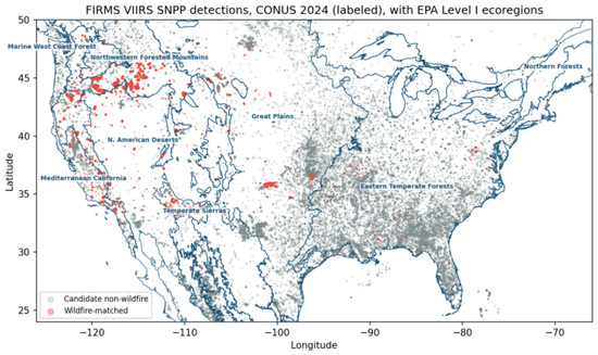
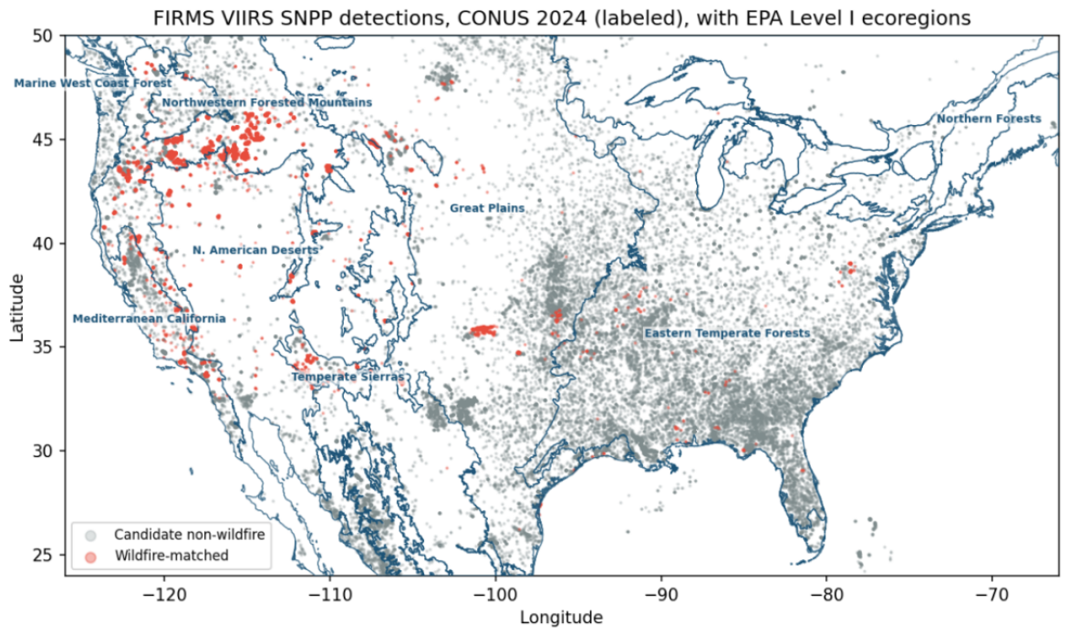
Three findings stand out. First, the random split (F1 = 0.985) overstates event-aware performance (F1 = 0.767) by 0.218 absolute: detections from the same incident leak across folds. Second, under the spatial-block holdout—transfer to entirely unseen regions—adding raw coordinates reduces F1 from $0.818$ to $0.627$. A feature that helps in-distribution but hurts out-of-region is the textbook signature of memorization [19]. Third, the coordinate-free model is far more stable across regimes (F1 $0.75$–$0.89$) than the coordinate model (F1 $0.63$–$0.99$). Figure 2 shows why: wildfire-matched detections concentrate in the West while candidate negatives blanket the agricultural East, so longitude alone is highly predictive within 2024 CONUS but does not encode wildfire physics. The overlaid EPA Level I ecoregion boundaries in Figure 2 make the mechanism concrete: wildfire-matched detections concentrate in the Northwestern Forested Mountains, Mediterranean California, and the North American Deserts, whereas the candidate negatives blanket the Great Plains and the Eastern Temperate Forests, where agricultural burning and industrial heat sources dominate the detection stream.

Figure 2. Labeled FIRMS VIIRS SNPP detections, CONUS 2024, with EPA Level I ecoregion boundaries (dark blue) overlaid; plotted sample $N=\mathrm{60,000}$ of 521,395 detections. Wildfire-matched (red) concentrate in the western U.S.; candidate non-wildfire (gray) dominate the agricultural East. This spatial structure makes raw longitude highly predictive in-sample but non-transferable.

To test whether the recommendation—coordinate-free, spatiotemporal-clustering features—actually generalizes, Table 6 extends the comparison to the GCC (causal trailing-window clustering, Section 3.4), with and without raw coordinates. The coordinate-free GCC is the most robust model under spatial transfer: it attains spatial-block F1 = 0.868, versus $0.818$ for coordinate-free LightGBM and only $0.627$ for the coordinate-using LightGBM. Adding causal clustering to the coordinate-free model improves spatial-block F1 from $0.818$ to $0.868$ and event-aware F1 from $0.748$ to $0.772$; both improvements exceed the bootstrap uncertainty (non-overlapping 95% CIs in Table 6). By contrast, clustering on top of raw coordinates yields little incremental robustness, because the coordinates already dominate (Section 4.8). This directly supports our deployment recommendation: drop raw coordinates, keep causal spatiotemporal density, and validate under spatial holdout.

Table 6. F1 by model and validation regime (balanced test; $N_{\mathrm{test}}$: event-aware 27,444, spatial-block 28,434, temporal 80,000); square brackets give bootstrap 95% CIs (1000 resamples), PR-AUC in parentheses. The best F1 in each validation regime (column) is shown in bold. Coordinate-free GCC generalizes best to unseen regions (spatial-block).

Model	Event-Aware	Spatial-Block	Temporal
LightGBM, with lat/lon	0.767 [0.761, 0.773] (0.92)	0.627 [0.619, 0.634] (0.83)	0.855 [0.852, 0.857] (0.95)
LightGBM, coordinate-free	0.748 [0.742, 0.755] (0.82)	0.818 [0.813, 0.823] (0.89)	0.805 [0.802, 0.807] (0.78)
GCC, with lat/lon	0.762 [0.756, 0.769] (0.92)	0.805 [0.800, 0.810] (0.93)	0.876 [0.873, 0.878] (0.95)
GCC, coordinate-free	0.772 [0.766, 0.777] (0.84)	0.868 [0.864, 0.873] (0.93)	0.829 [0.826, 0.832] (0.84)

4.3. Spatial-Block-Size Sensitivity

Because the spatial-block conclusion could in principle depend on the 5° block size, Table 7 repeats the spatial-block experiment with 2.5° and 10° blocks. For each size we report the primary split (seed 42, with bootstrap CIs) and the mean ± standard deviation of F1 across five random block-to-fold assignments, because with few groups the specific held-out regions matter.

Table 7. Spatial-block-size sensitivity (LightGBM, balanced test). “Primary split” is the seed-42 assignment used elsewhere in the paper, with bootstrap 95% CIs; “5 splits” reports mean ± SD of F1 over five random block-to-fold assignments. $N_{\mathrm{test}}$ (primary split): 35,884 (2.5°), 28,434 (5°), 24,672 (10°).

Block Size	Blocks	Features	F1, Primary Split	F1, 5 Splits	Worst Split
2.5°	218	with lat/lon	0.926 [0.923, 0.929]	0.73 ± 0.14	0.531
		coordinate-free	0.852 [0.848, 0.856]	0.81 ± 0.04	0.758
5°	65	with lat/lon	0.627 [0.619, 0.634]	0.81 ± 0.10	0.627
		coordinate-free	0.818 [0.813, 0.823]	0.85 ± 0.05	0.772
10°	20	with lat/lon	0.874 [0.870, 0.879]	0.38 ± 0.39	0.004
		coordinate-free	0.873 [0.869, 0.877]	0.56 ± 0.29	0.091

Three patterns emerge. First, at every block size the coordinate-free model achieves a higher mean F1 across splits and a substantially lower variance than the coordinate model (e.g., at 5°: $0.85\pm 0.05$ vs. $0.81\pm 0.10$; at 2.5°: $0.81\pm 0.04$ vs. $0.73\pm 0.14$). Second, small blocks partially reintroduce spatial leakage: at 2.5° many held-out blocks border training blocks, so the coordinate model can again exploit location (its primary-split F1 rises to $0.926$), which is precisely why coarse blocks are required for honest spatial evaluation [18]. Third, at 10° only 20 populated blocks remain and both models become unstable across assignments (worst-case F1 of $0.004$ with coordinates vs. $0.091$ coordinate-free when nearly the entire western fire region is held out)—a regime in which no location-agnostic feature set can compensate for the near-total absence of western fires in training. The 5° choice balances these two failure modes, and the paper’s qualitative conclusion—raw coordinates do not help, and typically hurt, spatial transfer—holds at every block size.

4.4. Clustering-Window Sensitivity

Table 8 varies the trailing-window lengths of the causal density features for the coordinate-free GCC, halving (3 h/12 h) and doubling (12 h/48 h) the default 6 h/24 h pair. F1 changes by at most $0.008$ under the event-aware regime and $0.006$ under the spatial-block regime, in most cases within the bootstrap CIs. The overpass-cadence-anchored default is therefore a reasonable, non-fragile choice, and the clustering signal reflects genuine multi-overpass persistence rather than a tuned window.

Table 8. Clustering-window sensitivity for the coordinate-free GCC (balanced test; $N_{\mathrm{test}}$: event-aware 27,444, spatial-block 28,434). Cells show F1 with bootstrap 95% CIs and PR-AUC in parentheses.

Trailing Windows	Event-Aware	Spatial-Block
3 h/12 h	0.764 [0.758, 0.770] (0.83)	0.867 [0.863, 0.871] (0.92)
6 h/24 h (default)	0.772 [0.766, 0.777] (0.84)	0.868 [0.864, 0.873] (0.93)
12 h/48 h	0.770 [0.764, 0.776] (0.84)	0.873 [0.869, 0.877] (0.93)

4.5. Confusion Matrix and Operating Point

Table 9 gives the LightGBM (full-feature) confusion matrix on the balanced event-aware test at $p\ge 0.5$. The realistic operating point is high precision (0.935) with moderate recall (0.650)—very different from the near-perfect random-split numbers.

Table 9. Confusion matrix: LightGBM (full features), event-aware test, $p\ge 0.5$ (balanced, 13,722 per class; $N=\mathrm{27,444}$).

	Predicted Non-Wildfire	Predicted Wildfire
True Non-Wildfire	13,107	615
True Wildfire	4807	8915

4.6. Threshold Analysis

Table 10 reports cumulative thresholds ($p\ge \tau$): each row is a single decision threshold with its precision, recall, FPR, and alert count. Table 11 then reports mutually exclusive tiers, clarifying the earlier ambiguity: the bottom tier’s 35.0% is the share of all true wildfires that fall into the low-priority bucket (missed-positive share), not a recall.

Table 10. Cumulative threshold analysis (LightGBM, event-aware test, $N=\mathrm{27,444}$). Each row applies a single threshold $p\ge \tau$.

$\mathit{\tau }$	Alerts	TP	FP	Prec	Rec	FPR
0.90	6957	6652	305	0.956	0.485	0.022
0.80	7892	7502	390	0.951	0.547	0.028
0.70	8481	8018	463	0.945	0.584	0.034
0.50	9530	8915	615	0.935	0.650	0.045
0.40	9995	9286	709	0.929	0.677	0.052

Table 11. Mutually exclusive priority tiers (LightGBM, event-aware test, $N=\mathrm{27,444}$). “% of all WF” is the share of all true wildfires captured by the tier; “% of all non-WF” the share of all negatives.

Tier	Det.	True WF	Prec	% of All WF	% of All Non-WF
High ($p\ge 0.80$)	7892	7502	0.951	54.7	2.8
Review ($0.5–0.8$)	1638	1413	0.863	10.3	1.6
Low ($p<0.50$)	17,914	4807	0.268	35.0	95.5

4.7. Ablation Study

Table 12 gives incremental feature-group contribution (LightGBM, event-aware). Satellite radiometric features alone reach only F1 = 0.644; temporal features (month/hour) add the largest credible gain (to $0.748$); adding raw coordinates lifts F1 only marginally ($0.767$) while inflating PR-AUC ($0.818\to 0.917$)—consistent with coordinates sharpening in-distribution ranking without improving transferable decisions (cf. Table 5).

Table 12. Incremental ablation (LightGBM, event-aware test, $N=\mathrm{27,444}$).

Features (Cumulative)	Prec	Rec	F1	PR-AUC
Satellite radiometric	0.676	0.615	0.644	0.712
+Engineered ($\Delta T$, logFRP)	0.674	0.614	0.643	0.713
+Temporal (month, hour)	0.815	0.692	0.748	0.818
+Geographic (lat, lon)	0.935	0.650	0.767	0.917

4.8. Feature Importance

Figure 3 and Table 13 show LightGBM importance.

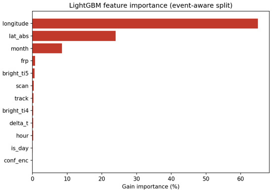
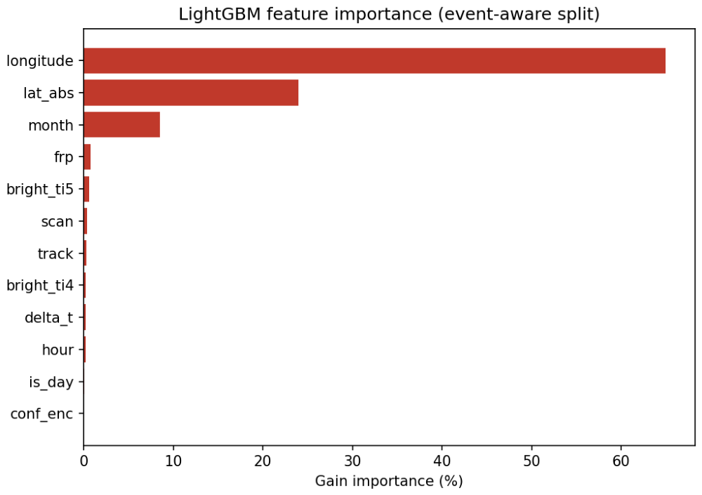
Figure 3. LightGBM gain importance (event-aware split; test $N=\mathrm{27,444}$). Geographic and temporal features dominate; radiometric features contribute little.

Table 13. Top features (LightGBM, event-aware; permutation importance computed on the test set, $N=\mathrm{27,444}$). Gain % is each feature’s share of the model’s total split-gain, normalized to sum to 100% over all 14 features (remaining low-gain features are omitted from the table). Group totals, obtained by summing member-feature shares: geographic 88.9% (longitude 65.0 + |latitude| 23.9 + latitude 0.0), temporal 8.7%, satellite 2.2%, engineered 0.2%.

Feature	Gain %	Permutation $\mathbf{\Delta }$F1
longitude	65.0	0.324
|latitude|	23.9	0.220
month	8.5	0.147
FRP	0.7	0.016
bright_ti5	0.6	0.010
scan	0.4	−0.001
bright_ti4	0.2	0.003

Calculation of the Gain Shares

Because the statement “geographic coordinates account for 88.9% of model gain” is used repeatedly in this paper, we state its calculation explicitly. Gain here is LightGBM’s native split-gain importance: for each feature j, the fitted event-aware full-feature model reports $G_j$, the total reduction in the training objective (binary log-loss) summed over every tree split that uses feature j. We normalize by the total over all $d=14$ features, so feature j’s gain share is $100\times G_j/{\sum }_{k=1}^d{G}_k$; the “Gain %” column of Table 13 therefore sums to 100% across all features. A group share is the sum of its member features’ shares. The geographic group comprises three features, and its 88.9% total is their sum: longitude (65.0%) +|latitude| (23.9%) + raw latitude (0.0%; the fitted model never splits on raw latitude because |latitude| subsumes it). Two clarifications follow from this definition. First, the 88.9% is a relative attribution within a single trained model—the share of that model’s total loss reduction assigned to coordinate splits—not a performance improvement measured against a coordinate-free reference model. Second, the complementary “improvement over a baseline” view is provided by the incremental ablation of Table 12, where adding the geographic group to the radiometric+engineered+temporal model changes F1 from 0.748 to 0.767 and PR-AUC from 0.818 to 0.917, and by the with/without-coordinate comparison of Table 5. The two views are consistent: coordinates absorb most of the model’s internal structure (gain share) while adding modest in-distribution benefit and harming spatial transfer.

Geography dominates: longitude (65.0% gain), |latitude| (23.9%), and month (8.5%) together account for 97.4% of gain; the entire satellite group contributes only 2.2%. Permutation importance (F1 drop) confirms the ordering. This quantifies the leakage mechanism: the model primarily learns where 2024 fires were. Section 5 discusses why the radiometric group contributes so little in this task.

4.9. Calibration

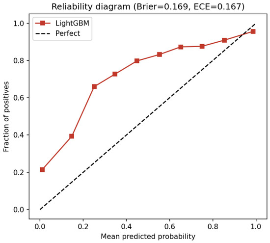
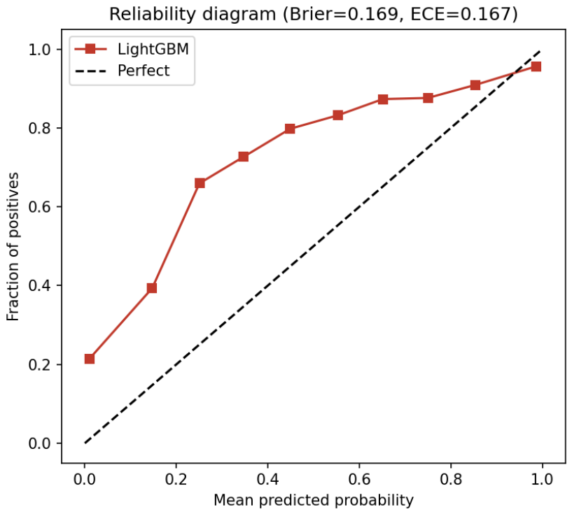
On the event-aware test, the gradient-boosted models are poorly calibrated under the implied spatial distribution shift: LightGBM has Brier = 0.169 and expected calibration error (ECE) = 0.167 (Figure 4); causal GCC is essentially identical (Brier = 0.169). Probabilities from these models should therefore not be read as analyst-facing confidences without post hoc recalibration [21].

Figure 4. Reliability diagram (LightGBM, event-aware test, $N=\mathrm{27,444}$). Deviation from the diagonal reflects miscalibration under spatial distribution shift.

4.10. Natural-Prevalence Evaluation

Evaluated on all held-out event-group detections (98,071; 14.0% positive), LightGBM precision falls from 0.935 (balanced) to 0.692, with recall 0.650, F1 0.670, and PR-AUC 0.691. Because most operational FIRMS detections are non-wildfire, real-world alert precision and analyst workload are markedly worse than balanced-set metrics suggest; this gap must be stated for any deployment claim.

Why 14.0% and Not 25.3%?

The global positive rate is 25.3%, but the held-out test groups are 14.0% positive (training groups are 27.9%). This is expected variance of event-aware grouping: positives are concentrated in 1067 incidents, and whole incidents are assigned to a fold, so the test prevalence depends on which incidents land in test. Here the 217 held-out incidents are smaller on average (63.2 detections each) than training incidents (138.9 each), while candidate negatives—grouped across many 0.5° tiles—distribute more evenly. Fewer positive detections per held-out incident therefore lowers test prevalence below the global rate. We report metrics on the actual held-out groups rather than assuming the global prevalence.

4.11. Label-Buffer Sensitivity

Positives are defined by a 1 km buffer, yet the top false positives (discussed in Section 4.13) sit 6–10 km from a perimeter and are plausibly fire-related—i.e., buffer-induced label noise. Table 14 varies the buffer over $\{500\mathrm{m},1,2,5\}$ km (event-aware split). Results are highly buffer-sensitive: a tight 500 m buffer collapses LightGBM-full F1 to 0.598 (many near-perimeter positives mislabeled), whereas the coordinate-free GCC is far more stable (0.845), and a 2 km buffer is the most favorable for both. The positive count grows only modestly (130.5 k→146.4 k), so the 6–10 km false positives remain candidate negatives even at 5 km—confirming residual label noise that no single buffer removes. This buffer dependence is a genuine source of uncertainty in all reported metrics, which is why we anchor the 1 km choice to the positional error budget of the match (Section 3.2.1) rather than to classifier performance, and why we report this sweep alongside all headline results.

Table 14. Label-buffer sensitivity (event-aware split; balanced test at each buffer, $N\approx \mathrm{27,000}$–$\mathrm{29,000}$); cells show F1 (PR-AUC). LightGBM uses full features; GCC is coordinate-free. Positives and prevalence shift modestly; metrics shift substantially.

Buffer	Positives	Prevalence	LightGBM (Full)	GCC (Coordinate-Free)
500 m	130,501	25.0%	0.598 (0.91)	0.845 (0.90)
1 km	131,771	25.3%	0.767 (0.92)	0.772 (0.84)
2 km	134,411	25.8%	0.850 (0.96)	0.871 (0.90)
5 km	146,414	28.1%	0.812 (0.86)	0.776 (0.82)

4.12. Error Analysis

Table 15 reports error rates by confidence class and day/night (land-cover-stratified error analysis is deferred pending NLCD integration; Section 5.10). False-negative rate is far higher in daytime (0.457 vs. 0.258 at night) and at low confidence (0.556), reflecting both faint daytime signals and the model’s geographic prior.

Table 15. Error rates (LightGBM, event-aware test, $p\ge 0.5$; total $N=\mathrm{27,444}$; per-category N in the last column).

Category	FP Rate	FN Rate	N
Conf: Low	0.046	0.556	1540
Conf: Nominal	0.044	0.343	24,334
Conf: High	0.056	0.236	1570
Day	0.032	0.457	13,717
Night	0.059	0.258	13,727

4.13. Qualitative Failures

Table 16 illustrates the geographic bias concretely. The top false positives are clustered detections in the northern Mountain West only 6–10 km from a wildfire perimeter (likely fire-related but just outside the 1 km buffer—i.e., label noise), which the model confidently calls wildfire ($p=1.0$). The false negatives are genuine eastern U.S. wildfires (0–1 km from a perimeter) that the model assigns $p=0.0$, because it learned that wildfires are a western phenomenon. This is exactly the failure mode that spatial-block validation exposes.

Table 16. Representative errors (LightGBM, event-aware test; $N=6$ examples, the three highest-confidence false positives and three lowest-probability false negatives). Coordinates rounded to 0.1°. “Dist” is distance to nearest 2024 wildfire perimeter.

Type	Region	Lat, Lon	Date	FRP	Conf	D/N	p	Dist (km)
FP	N. Mountain West	44.4, −113.9	2 October 2024	2.4	nominal	night	1.00	10.2
FP	N. Mountain West	44.3, −113.9	30 September 2024	1.9	nominal	night	1.00	6.6
FP	N. Mountain West	44.4, −113.9	29 September 2024	2.1	nominal	night	1.00	9.2
FN	N. Eastern U.S.	40.8, −75.6	2 November 2024	6.2	nominal	day	0.00	0.0
FN	S. Eastern U.S.	30.7, −82.1	3 February 2024	8.1	nominal	day	0.00	1.0
FN	S. Eastern U.S.	35.8, −82.1	6 December 2024	1.5	nominal	night	0.00	0.0

4.14. ROC and PR Curves

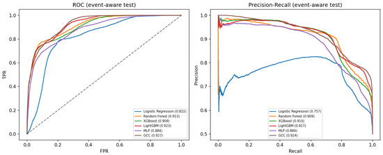
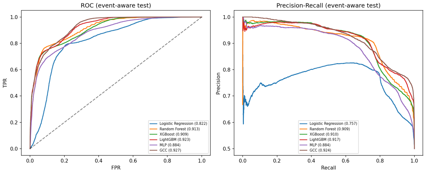
Figure 5 shows ROC and PR curves on the event-aware test; the gradient-boosted models lead narrowly and all ML models separate clearly from chance, but the gap from the random-split regime is substantial.

Figure 5. ROC (left) and precision–recall (right) curves on the event-aware test set ($N=\mathrm{27,444}$). The gradient-boosted models (LightGBM, causal GCC) attain the highest AUCs, closely followed by Random Forest.

5. Discussion

5.1. Does ML Improve over Baselines?

Yes, substantially, but the margin depends entirely on the evaluation protocol. Under the primary event-aware split, tree models reach F1 $\approx 0.76$–$0.78$ versus the best discriminative baseline (FRP threshold, F1 = 0.426) and FIRMS high-confidence thresholding (F1 = 0.128, recall = 0.071). FIRMS high confidence is highly specific (0.957) but misses 93% of wildfire-matched detections; the ≥nominal variant recovers recall only by sacrificing precision to chance. Contextual ML clearly helps—but the headline F1 = 0.985 reported under random splitting is not a valid estimate of operational performance.

5.2. Which Features Matter, and Why Is That a Problem?

Raw geographic coordinates account for 88.9% of LightGBM gain (the summed split-gain share of the three coordinate features within the full-feature model, as defined in Section 4.8), with temporal features second (8.7%) and radiometric features negligible (2.2%). Coordinates improve in-distribution ranking (PR-AUC $0.818\to 0.917$) but degrade transfer to unseen regions (spatial-block F1 $0.818\to 0.627$). We do not claim that geographic information is meaningless. Latitude and longitude partly proxy stable, fire-relevant environmental gradients—climate, fuel type and continuity, and human ignition patterns—so some of the coordinate signal is genuine. The problem is representational: a tree model given raw coordinates encodes those gradients as a lookup table of where 2024 fires occurred, which is exactly the component that fails to transfer (Table 7). Under the current single-year experimental setting we cannot fully separate “legitimate but location-correlated environment” from “pure memorization”; what we can show is that whatever the mixture, raw coordinates harm out-of-region performance while coordinate-free variants do not. The constructive resolution is to replace raw coordinates with the transferable covariates they proxy—weather, fuels, terrain, and land cover—which is the top priority of our future work (Section 5.11).

5.3. Why Do Radiometric Features Contribute So Little?

The near-zero contribution of the radiometric group (2.2% of gain) deserves explanation, since it may seem counterintuitive for a thermal-detection problem. First, every candidate in our dataset has already passed the VIIRS active fire detection test, which is itself a contextual radiometric algorithm [4]: conditioning on detection truncates precisely the radiometric variation that separates fire from non-fire background, leaving a selection-biased remnant with limited incremental information. Second, the radiometric distributions of wildfire and non-wildfire detections overlap heavily: a smoldering wildfire edge pixel and an agricultural burn can both present 1–5 MW FRP at similar brightness temperatures [5], and gas flares are engineered to burn persistently at wildfire-like intensities [6]. What distinguishes a wildfire incident is therefore less the instantaneous radiometry of a single pixel than its context—temporal persistence, spatial density and growth—which is exactly why the causal-clustering features and the month/hour features carry most of the transferable signal.

5.4. Is Clustering the Answer? Only if It Is Causal

Spatiotemporal clustering is a physically motivated, location-agnostic signal, but its benefit is easy to overstate. With non-causal full-partition clustering, GCC appeared to reach F1 = 0.908; this counts detections from the entire test period (including the future) and is a second leakage path. With causal trailing-window density, GCC ties plain LightGBM in-distribution (F1 = 0.762 vs. 0.767). The genuine, defensible benefit appears only under spatial transfer and only without raw coordinates: causal-clustering, coordinate-free GCC attains spatial-block F1 = 0.868, the best of any configuration (Table 6), versus $0.627$ for the coordinate model. This benefit is insensitive to the window choice (Table 8). This is the configuration we recommend.

5.5. Where Does the Model Fail?

Failures are geographically and diurnally structured (Table 15 and Table 16). False negatives concentrate in the eastern U.S. and in daytime/low-confidence detections; false positives concentrate near—but just outside—western perimeters, partly reflecting 1 km label-buffer noise. Both patterns follow from the geographic prior quantified above and are invisible under random validation.

5.6. Comparison with Previously Reported Accuracies

Wildfire ML studies frequently report ROC-AUC above 0.9 or accuracy above 95% under random cross-validation—for example, susceptibility mapping with Random Forest [16], and many of the classification results surveyed by Jain et al. [11]. Our results suggest such figures should be interpreted in light of the validation protocol: our own random split produced F1 = 0.985, which fell to $0.767$ under event-aware and $0.627$ under spatial-block evaluation. This is consistent with the systematic inflation documented for spatially autocorrelated data by Ploton et al. [17] and Kattenborn et al. [20], and with the coordinate-memorization mechanism of Meyer et al. [19]. We emphasize that this does not invalidate prior studies whose goal is within-region interpolation, where random or proximity-based validation can be appropriate for the intended use [18]. But for operational FIRMS triage—where a deployed model must handle regions and seasons underrepresented in training—leakage-controlled spatial and event-aware holdouts are the appropriate yardstick, and we encourage authors of high-accuracy wildfire classifiers to report at least one spatial-holdout figure alongside random-CV results.

5.7. Operational Tradeoffs

For emergency management the precision–recall tradeoff is asymmetric: missed wildfires are costlier than false alarms, yet false alarms drive cry-wolf fatigue [7]. The tier analysis (Table 11) supports a triage workflow—a high-confidence tier capturing 54.7% of wildfires at 0.951 precision, a small human-review tier, and a low-priority tier—but the natural-prevalence result (precision 0.692 at 14% prevalence; Section 4.10) shows real alert volumes and precision are worse than balanced metrics imply.

5.8. Operational Integration

Concretely, we envision the model as a ranking layer inside an emergency-management common operating picture (e.g., the platforms used by state and federal fire-duty officers), not as an autonomous alerting system. Incoming FIRMS detections would be scored within minutes of each overpass using only past data (the causal design guarantees this is feasible in production), then deduplicated to incident-level items via the same ∼2 km trailing-window clusters used as features. The three tiers of Table 11 map onto analyst workflow as follows: high-tier clusters ($p\ge 0.8$) are placed at the top of the analyst review queue with map context (nearby known incidents, recent detection history, land ownership); review-tier clusters are batched for periodic sweeps; and low-tier detections are logged and searchable but not surfaced. At natural prevalence, roughly 13% of the incoming stream exceeds $p\ge 0.5$ (about 190 of the ∼1400 average daily CONUS detections in 2024), of which about 69% are wildfire-matched—a volume compatible with human review once detections are collapsed to clusters. Two safeguards are mandatory given our findings: probabilities must be recalibrated (e.g., isotonic regression on a held-out event-aware fold) before being displayed as confidences, because the raw outputs are miscalibrated (ECE = 0.167), and the deployed feature set must be the coordinate-free causal-clustering variant validated under spatial holdout, since the coordinate model’s failure mode—systematically dismissing fires in historically low-fire regions—is operationally unacceptable. Analyst dispositions (confirm/dismiss) should be logged to support periodic retraining and the human-in-the-loop evaluation planned in Section 5.11.

5.9. Decision Support, Not Automation

This system should serve as a prioritization layer. Human analysts must retain authority over incident classification, model outputs must include calibrated probabilities and explanatory context, and—given the demonstrated leakage—deployment must use coordinate-free, spatiotemporal features validated under spatial holdout.

5.10. Limitations

• Feature scope: This evaluation uses only VIIRS radiometric, temporal, and geographic features. Weather, land-cover, and terrain layers are not integrated; we make no claim about their effect, and the title reflects only the features measured. In particular, wildfire occurrence and spread are driven by environmental variables absent here—elevation, slope, aspect, wind, fuel moisture, and vegetation continuity—so our conclusions characterize what is achievable from the FIRMS detection stream alone, not general wildfire classification with full environmental drivers. The relative ordering of feature families could change once such covariates are added, although the methodological finding (leakage-controlled validation is required) is independent of the feature set.
• Spatial leakage: Raw coordinates inflate in-distribution metrics; we report coordinate-free and spatial-block results as the honest performance estimates and recommend them for deployment.
• Label uncertainty: A 1 km spatial buffer (no full discovery/containment window, as NIFC records expose only current-perimeter dates) introduces both false positives just outside perimeters and candidate-negative noise from unreported fires.
• Class balance: Comparison metrics use balanced sampling; the natural-prevalence evaluation (14% positive) is the more realistic operating estimate.
• Scope: CONUS 2024, VIIRS SNPP only. Results may not generalize across years, sensors (MODIS), or regions. The single-year design has specific consequences. First, the 2024 fire geography is one draw from an interannually variable distribution: fire seasons differ in timing, regional emphasis, and severity, so a coordinate-using model trained on 2024 would degrade in a year whose fires concentrate elsewhere—the cross-year analog of the spatial-block failure we measured within 2024. Second, our temporal holdout (train January–August, test September–December) spans only within-year seasonal shift, which is milder than between-year climate shift; multi-year training with leave-one-year-out validation (e.g., train 2020–2023, test 2024) is the natural extension and is enabled by the NIFC 2020–2024 archive we already hold. Third, we expect the qualitative conclusions to persist under multi-year data, because their mechanism—spatial autocorrelation of fire occurrence and the resulting memorization incentive—operates across years as well as within them; multi-year training should, if anything, further penalize raw coordinates (fire locations vary between years while physics does not) and favor persistence-based features. This expectation is, however, a hypothesis to be tested, not a demonstrated result.
• Land-cover error analysis: Deferred pending NLCD integration.
• No analyst validation/no autonomous use: The model has not been tested in a live workflow and is not validated for public alerts or autonomous decisions.

5.11. Future Work

The clearest path forward is to replace the memorization-prone geographic coordinates with the transferable environmental covariates they proxy, and to broaden the validation scope:

• Weather integration. Join ERA5/HRRR reanalysis at detection time and location to derive fire-weather covariates (temperature, relative humidity, wind speed, precipitation deficit, and composite indices such as hot–dry–windy). These are location-agnostic and physically causal, and should recover much of the legitimate signal currently entangled with raw coordinates.
• Vegetation and land cover. Integrate NLCD land-cover class and LANDFIRE fuel models to distinguish agricultural, urban-industrial, and wildland contexts directly—replacing the model’s current implicit “east = agriculture” longitude heuristic with an explicit, transferable covariate—and to enable the deferred land-cover-stratified error analysis.
• Topography. Add elevation, slope, and aspect from SRTM; slope-driven spread and terrain-constrained ignition patterns are established wildfire drivers whose absence limits the present feature space.
• Multi-year and multi-sensor evaluation. Extend to 2020–2024 with leave-one-year-out validation to test cross-year transfer under differing climate conditions and fire distributions, and add VIIRS NOAA-20/21 and MODIS streams to test cross-sensor robustness.
• Multi-class labeling. Move beyond binary labels to wildfire/prescribed burn/agricultural/industrial/other, using additional registries (e.g., prescribed-burn permits), which would sharpen both training signal and analyst-facing explanations.
• Human-in-the-loop evaluation and calibration. Deploy the recommended coordinate-free causal-clustering configuration in a shadow-mode analyst workflow (Section 5), recalibrate probabilities on event-aware folds, and measure analyst workload, override rates, and time-to-confirmation against the current FIRMS confidence baseline.

6. Conclusions

We presented a leakage-controlled empirical evaluation of contextual features for classifying FIRMS VIIRS SNPP thermal anomalies as wildfire incidents in CONUS 2024, using 521,395 detections matched to 3766 NIFC wildfire perimeters across 1067 incidents. Our central finding is methodological: a naive random split reports F1 = 0.985, but event-aware splitting reduces this to $0.767$ and a 5° spatial-block holdout to $0.627$, and feature attribution shows geographic coordinates (88.9% of gain, i.e., the coordinate features’ summed share of the model’s total split-gain; Section 4.8) memorize where 2024 fires occurred—removing them improves cross-region F1 from $0.627$ to $0.818$. We further show that spatiotemporal clustering must be causal: full-partition clustering inflates GCC to F1 = 0.908 by leaking future detections, whereas a causal trailing-window version ties plain LightGBM in-distribution ($0.762$). The most robust configuration under spatial transfer is causal clustering without raw coordinates (spatial-block F1 = 0.868). Bootstrap confidence intervals confirm that these protocol- and feature-induced gaps far exceed statistical uncertainty, and sensitivity analyses show they are robust to the spatial-block size (2.5°–10°) and to the clustering-window lengths. Under natural prevalence, precision drops to 0.69, and results vary with the labeling buffer. We conclude that contextual ML genuinely improves over FIRMS radiometric baselines, but that spatial leakage—not raw accuracy—is the key obstacle to credible, generalizable wildfire-incident classification. These conclusions apply to the radiometric, temporal, and spatiotemporal feature space evaluated here; integrating weather, vegetation, topographic, and land-cover variables, extending to multi-year and multi-sensor data, adding multi-class labels, and conducting human-in-the-loop analyst evaluation are detailed as future work in Section 5.11.

References

- Bowman, D.M.; Balch, J.K.; Artaxo, P.; Bond, W.J.; Carlson, J.M.; Cochrane, M.A.; D’Antonio, C.M.; DeFries, R.S.; Doyle, J.C.; Harrison, S.P.; et al. Fire in the Earth system. Science 2009, 324, 481–484. [Google Scholar] [CrossRef] [Scilit] [PubMed]
- Jolly, W.M.; Cochrane, M.A.; Freeborn, P.H.; Holden, Z.A.; Brown, T.J.; Williamson, G.J.; Bowman, D.M.J.S. Climate-induced variations in global wildfire danger. Nat. Commun. 2015, 6, 7537. [Google Scholar] [CrossRef] [Scilit] [PubMed]
- Giglio, L.; Schroeder, W.; Justice, C.O. The collection 6 MODIS active fire detection algorithm. Remote Sens. Environ. 2016, 178, 31–41. [Google Scholar] [CrossRef] [Scilit] [PubMed]
- Schroeder, W.; Oliva, P.; Giglio, L.; Csiszar, I.A. The new VIIRS 375m active fire detection data product: Algorithm description and initial assessment. Remote Sens. Environ. 2014, 143, 85–96. [Google Scholar] [CrossRef] [Scilit]
- McCarty, J.L.; Justice, C.O.; Korontzi, S. Agricultural burning in the southeastern United States detected by MODIS. Remote Sens. Environ. 2007, 108, 151–162. [Google Scholar] [CrossRef] [Scilit]
- Elvidge, C.D.; Zhizhin, M.; Baugh, K.; Hsu, F.-C.; Ghosh, T. Methods for global survey of natural gas flaring from visible infrared imaging radiometer suite data. Energies 2016, 9, 14. [Google Scholar]
- LeClerc, J.; Joslyn, S. The cry wolf effect and weather-related decision making. Risk Anal. 2015, 35, 385–395. [Google Scholar] [CrossRef] [Scilit] [PubMed]
- Giglio, L.; Descloitres, J.; Justice, C.O.; Kaufman, Y.J. An enhanced contextual fire detection algorithm for MODIS. Remote Sens. Environ. 2003, 87, 273–282. [Google Scholar] [CrossRef] [Scilit]
- Artés, T.; Oom, D.; de Rigo, D.; Durrant, T.H.; Maianti, P.; Libertà, G.; San-Miguel-Ayanz, J. A global wildfire dataset for the analysis of fire regimes and fire behaviour. Sci. Data 2019, 6, 296. [Google Scholar] [CrossRef] [Scilit] [PubMed]
- Andela, N.; Morton, D.C.; Giglio, L.; Paugam, R.; Chen, Y.; Hantson, S.; van der Werf, G.R.; Randerson, J.T. The Global Fire Atlas of individual fire size, duration, speed and direction. Earth Syst. Sci. Data 2019, 11, 529–552. [Google Scholar] [CrossRef] [Scilit]
- Jain, P.; Coogan, S.C.P.; Subramanian, S.G.; Crowley, M.; Taylor, S.W.; Flannigan, M.D. A review of machine learning applications in wildfire science and management. Environ. Rev. 2020, 28, 478–505. [Google Scholar] [CrossRef] [Scilit]
- Grinsztajn, L.; Oyallon, E.; Varoquaux, G. Why do tree-based models still outperform deep learning on tabular data? In Proceedings of the Advances in Neural Information Processing Systems (NeurIPS) Datasets and Benchmarks Track, New Orleans, LA, USA, 28 November–9 December 2022. [Google Scholar]
- Breiman, L. Random forests. Mach. Learn. 2001, 45, 5–32. [Google Scholar] [CrossRef] [Scilit]
- Chen, T.; Guestrin, C. XGBoost: A scalable tree boosting system. In Proceedings of the 22nd ACM SIGKDD International Conference on Knowledge Discovery and Data Mining, San Francisco, CA, USA, 13–17 August 2016; pp. 785–794. [Google Scholar]
- Ke, G.; Meng, Q.; Finley, T.; Wang, T.; Chen, W.; Ma, W.; Ye, Q.; Liu, T. LightGBM: A highly efficient gradient boosting decision tree. In Proceedings of the Advances in Neural Information Processing Systems (NeurIPS), Long Beach, CA, USA, 4–9 December 2017; pp. 3146–3154. [Google Scholar]
- Tonini, M.; D’Andrea, M.; Biondi, G.; Degli Esposti, S.; Trucchia, A.; Fiorucci, P. A machine learning-based approach for wildfire susceptibility mapping. The case study of the Liguria region in Italy. Geosciences 2020, 10, 105. [Google Scholar] [CrossRef] [Scilit]
- Ploton, P.; Mortier, F.; Réjou-Méchain, M.; Barbier, N.; Picard, N.; Rossi, V.; Dormann, C.; Cornu, G.; Viennois, G.; Bayol, N.; et al. Spatial validation reveals poor predictive performance of large-scale ecological mapping models. Nat. Commun. 2020, 11, 4540. [Google Scholar] [CrossRef] [Scilit] [PubMed]
- Roberts, D.R.; Bahn, V.; Ciuti, S.; Boyce, M.S.; Elith, J.; Guillera-Arroita, G.; Hauenstein, S.; Lahoz-Monfort, J.J.; Schröder, B.; Thuiller, W.; et al. Cross-validation strategies for data with temporal, spatial, hierarchical, or phylogenetic structure. Ecography 2017, 40, 913–929. [Google Scholar] [CrossRef] [Scilit]
- Meyer, H.; Reudenbach, C.; Wöllauer, S.; Nauss, T. Importance of spatial predictor variable selection in machine learning applications. Ecol. Model. 2019, 411, 108815. [Google Scholar] [CrossRef] [Scilit]
- Kattenborn, T.; Schiefer, F.; Frey, J.; Feilhauer, H.; Mahecha, M.D.; Dormann, C.F. Spatially autocorrelated training and validation samples inflate performance assessment of convolutional neural networks. ISPRS Open J. Photogramm. Remote Sens. 2022, 5, 100018. [Google Scholar] [CrossRef] [Scilit]
- Niculescu-Mizil, A.; Caruana, R. Predicting good probabilities with supervised learning. In Proceedings of the 22nd International Conference on Machine Learning (ICML), Bonn, Germany, 7–11 August 2005; pp. 625–632. [Google Scholar]
Disclaimer/Publisher’s Note: The statements, opinions and data contained in all publications are solely those of the individual author(s) and contributor(s) and not of MDPI and/or the editor(s). MDPI and/or the editor(s) disclaim responsibility for any injury to people or property resulting from any ideas, methods, instructions or products referred to in the content. |
© 2026 by the authors. Licensee MDPI, Basel, Switzerland. This article is an open access article distributed under the terms and conditions of the Creative Commons Attribution (CC BY) license.