Using the Response Surface Method for the Optimization of Gas-Phase Hydrogenation of Carbon Dioxide on Nickel-Based Catalysts—A Large Laboratory-Scale Process

Abstract

In this study, the response surface method (RSM) was used to determine the best reaction conditions for the gas-phase hydrogenation of carbon dioxide on a commercial nickel-based catalyst. The RSM was applied in our previous study to find the optimal conditions for the same process carried out in laboratory-scale tubular reactors. The main benefits observed were fast detection of optimal conditions and the high precision of the optimum detected (which was experimentally confirmed). These advantages were due to the small number of experiments conducted and the simplicity of the models employed; only linear and quadratic models were developed. The successful result encouraged us to carry out experiments in a larger-scale reactor—an intermediate between a laboratory plant and a pilot plant. This approach helped us to fix some problems resulting from the larger scale of the process conducted. Despite the difficulties described in the main part of this article, we can recommend using the RSM as a tool for supporting experimentation and substantially speeding up the analysis of results and their introduction into practice. At the process scale considered, maximum carbon dioxide conversion was obtained at a temperature of 354 °C and a ratio of molar fluxes of H₂ to CO₂ equal to 3.9. It should be emphasized that this result was confirmed experimentally.

1. Introduction

The processes in which hydrogen takes part are playing an increasingly larger role in energy transformation. To achieve the expected outcomes with respect to stopping environmental pollution and climate change, an experiment on a larger scale is necessary. In research and development (R&D) investigations, it is assumed that experiments will be conducted beyond the laboratory scale to reach higher Technology Readiness Levels (TRLs). The larger scale of experiments entails greater costs of investigations to reduce the number of experiments. Our previous study [1] showed that applying the response surface methodology (RSM) to the gas-phase hydrogenation of carbon dioxide can help determine the optimal conditions of the process carried out. The successful result achieved encouraged us to carry out experiments in a larger-scale reactor.

Increasing process scale is a very important issue from a technological point of view. Processes realized at the laboratory scale exhibit different behaviors relative to the same processes realized at larger scales. The gas-phase hydrogenation of carbon dioxide on a nickel catalyst can be included in this category. At larger scales, the hydrodynamics of the flux of a reaction mixture more significantly influence the process, which can result in a change in the optimal conditions of the process in question. To confirm this hypothesis, we carried out the investigations presented in the main part of this article.

We will now briefly recapitulate information on the process considered and the RSM method. There is no uniform RSM approach. The RSM is a multistep procedure that explores relationships between independent variables (factors that can be controlled) and one or more dependent variables. Few initial steps are taken to help locate the rough region where the extreme value of the dependent variable lies, and the last one precisely localizes it. The objective to be established using RSM is defined by the researcher, so statistical and mathematical techniques should be selected depending on the problem to be solved. If the assumed objective was not achieved, the procedure should be repeated. This can be stated in other words. Starting from some experimental results, a simple, empirical-type mathematical model is developed. This model designates conditions for a new experiment, and then the next model is developed, and so on. Experiments and analyses are repeated sequentially to develop an appropriate model that is precise enough to realize the intentions of the researcher. It must be underlined that first- or second-order polynomials are most often used for model building (for empirical models). The structure of an empirical model does not require knowledge of the theoretical background of the process (in this case, the hydrogenation mechanism, kinetic equation, mass or heat transfer resistances, and so on). The influence of such factors is taken into account ‘as is’ from experiments. Because RSM does not require the determination of a kinetic equation or mass and heat transfer coefficients, it seems to be an ideal tool for the rapid optimization of complex heterogeneous processes. The RSM theory and applied methods have not changed relative to our previous study [1]. We used the Box and Wilson method [2] since it was developed to optimize processes in the chemical industry. We also used the RSM approach presented in the work of D. C. Montgomery and R. H. Myers [2,3]. This approach is broadly used for chemical and nonchemical processes, as discussed in detail in [1].

The gas-phase hydrogenation of carbon dioxide is a very promising process; however, in the literature, the results mainly concern the fundamentals of the process. Despite its favorable thermodynamics, the Sabatier reaction has to overcome large kinetic barriers to proceed. Additionally, ‘green’ hydrogen is more expensive than traditionally produced hydrogen. This results in poor microeconomic indicators that presently limit the application of the process in real life. However, these facts have also provoked numerous research institutions to conduct studies on this process. Review articles [4,5,6,7,8,9,10,11] present the fundamentals of conducting the process. Additional information on the mechanisms of CO₂ hydrogenation was presented by Jalama [12]. He critically reviewed the numerous mechanisms of CO₂ hydrogenation proposed in the literature over Ni and other metals and discussed the effect of catalyst properties and operating conditions on reaction kinetics. In his review, published kinetic models for CO₂ and research data on methanation are collected. His work confirms that there is no agreement among scientists on mechanisms and kinetics. A thermodynamic analysis of methane synthesis via the hydrogenation of carbon dioxide was performed. Ioelovich, in his work [13], claims that although the standard Gibbs potential of this reaction, known as the Sabatier reaction, is negative, methane synthesis under standard conditions does not occur due to kinetic limitations. To overcome these kinetic limitations, a significant increase in temperature and pressure is necessary, along with a catalyst additive, and under real conditions, the Sabatier reaction strongly transitions into the synthesis of methane, which can also be seen in [1].

The general reaction equation is as follows:

$$\mathrm{C}{\mathrm{O}}_2+4{\mathrm{H}}_2\rightleftarrows \mathrm{C}{\mathrm{H}}_4+2{\mathrm{H}}_2\mathrm{O}\hspace{1em}\hspace{1em}∆{\mathrm{H}}_{298\mathrm{K}}=-165\mathrm{k}\mathrm{J}·{\mathrm{m}\mathrm{o}\mathrm{l}}^{-1},$$

(1)

One of the products is methane, a gas that is widely applicable in chemical syntheses or even as an energy source.

An experiment is part and parcel of progress in science and engineering. It is especially important in technical applications, where it is often an indispensable tool for confirming or rejecting a new or innovative technical solution. However, a successful result obtained at the laboratory scale does not guarantee success at a larger scale. Unfortunately, the scaling up of tasks is seldom researched in universities; the universities are not properly equipped, and such experiments are simply too expensive. However, our previous application of the RSM helped us determine the reaction conditions in a fairly simple way by combining modeling and experimental results. In the present work, we will try to verify the previously revealed advantages of the RSM in a larger-scale reactor, an intermediate between a laboratory plant and a pilot plant. This is the main objective of this work.

2. Experimental Section

2.1. Setup

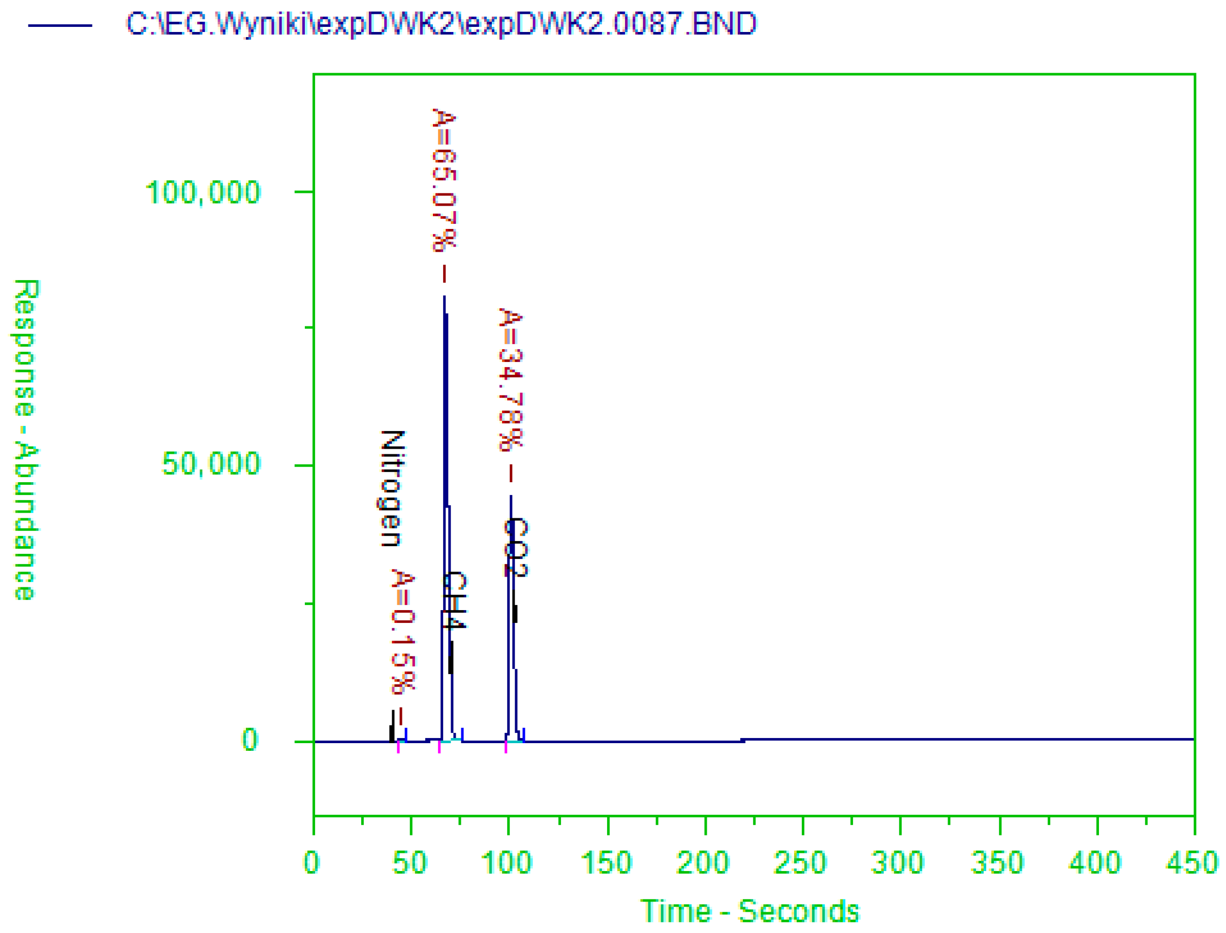
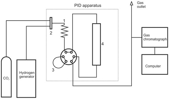
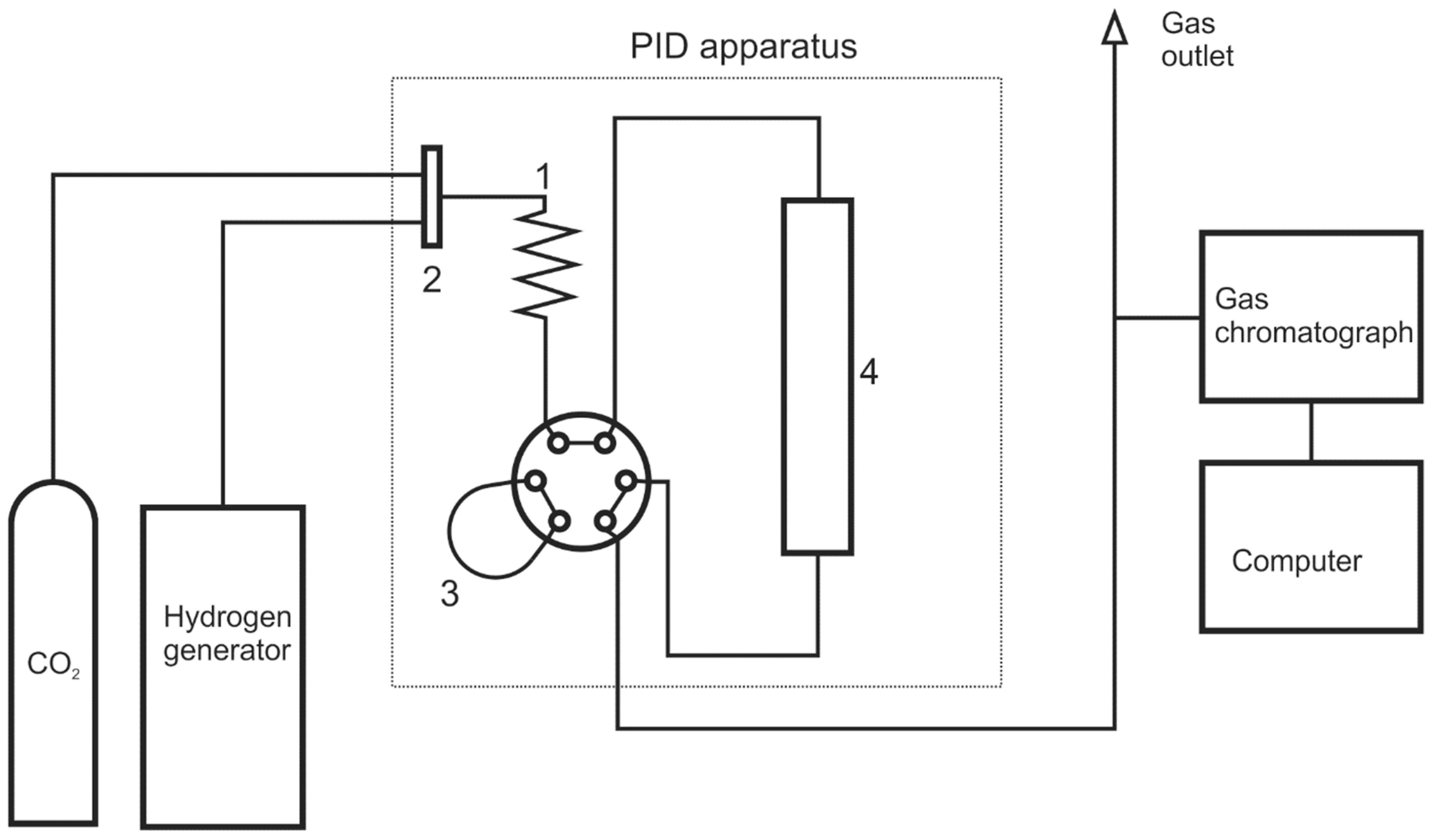
The same measurement system and procedures as described in detail in [1] were used. The system contains a Microactivity-Efficient Unit (manufacturer: Process Integral Development Eng&tech, Madrid, Spain) and a CALIDUS™ 101 Gas Chromatograph (manufacturer: Falcon Analytical, Lewisburg, WV, USA) equipped with a column with a length of 2.1 m, a gel diameter of 530 μm, and a thickness of 740 μm; a TCD detector; a hydrogen generator; and a CO₂ source. A scheme of the measurement system is presented in Figure 1. The only difference between this undertaking and the last one is that we used a tubular reactor with an inner diameter of 21 mm. The catalyst bed included 2.34 g of nickel catalyst (pellet diameter, 4–5 mm; nickel amount, <20%; manufacturer, INS, Puławy, Poland). The catalyst layer in the investigations presented in [1] included 0.6 g of nickel catalyst. The procedure for activating catalyst pellets recommended by the catalyst’s manufacturer was applied (details are given in [1]). The outlet gas stream was analyzed using gas chromatography when a steady state was achieved. Exemplary chromatogram, Figure A1, exported by the GC unit are included in Appendix A.

Figure 1. Scheme of the measurement system (1—pre-heater, 2—mass flow controllers, 3—bypass loop, and 4—tubular reactor).

2.2. RSM Procedure and General Conditions of the Experiments

As in our previous work, we determined the optimal reaction conditions in the following way: We searched for the highest level of CO₂ conversion possible under low-temperature and low-hydrogen/carbon dioxide molar flux ratio conditions. We examined an area of an excess of carbon dioxide (with respect to its stoichiometric value) at a low temperature (mild conditions). Here, we used the RSM and the central composite design method (CCD), as in our previous work. We used independent variables ‘x’ (reaction temperature, ‘x₁’, and hydrogen-to-carbon dioxide flux ratio at the reactor input, ‘x₂’) and the response of the system ‘y’ (carbon dioxide conversion, ‘y’). The x₁-value was measured directly, while the x₂-value was calculated as a proportion of the reactant fluxes, and the y-value was calculated using Equation (2).

$$\mathrm{y}=\left(1-{\displaystyle \frac{{\mathrm{S}}_{\mathrm{C}{\mathrm{O}}_2}}{{\mathrm{S}}_{\mathrm{C}{\mathrm{O}}_2}+{\mathrm{S}}_{\mathrm{C}{\mathrm{H}}_4}}}\right)·100\% ,$$

(2)

where ${\mathrm{S}}_{\mathrm{C}{\mathrm{O}}_2}$ is the peak area for carbon dioxide, and ${\mathrm{S}}_{\mathrm{C}{\mathrm{H}}_4}$ is the peak area for methane.

Note: Formula (2) is acceptable since the by-products were not observed; the chromatogram included confirmed that there were no by-products or intermediates in the post-reaction mixture.

Taking into account the technical data for the equipment presented, the experimental setup achieves precise and accurate measurements of up to 1 degree with respect to x₁ and up to 0.1 with respect to x₂. These physical limitations must be taken into account in the next steps. All results obtained ‘mathematically’ are rounded to the accuracy mentioned.

The amount of catalyst mentioned in Section 2.1 led to the same total flow rate and gas hourly space velocity (GHSV) (a parameter calculated as the volumetric flow rate divided by the volume of the catalyst bed) as given in [1]. The total flow rate of the reactants at the reactor inlet was constant and equal to 1 × 10⁻⁶ [m³ s⁻¹] (60.0 mL/min) at STP (STP = standard temperature and pressure, 273.15 [K] and 100,000 [Pa]). The flux consisted of hydrogen and carbon dioxide fluxes that were mixed. The GHSV value was equal to 2058 [h⁻¹]. These conditions are common for all experiments.

3. Results and Discussion

3.1. Level 1

According to the procedure presented in [2,3], the region where the highest degree of carbon dioxide conversion can appear was roughly determined using a first-order model. In the first step, the set of initial ranges of variables x₁ (temperature) and x₂ (hydrogen-to-carbon dioxide flux ratio at the reactor input) must be set. We employed the same independent variables as used previously [see Ref. [1], Table 1]. Carbon dioxide conversion was determined experimentally. The data and results pertaining to the experiment are presented in Table 1. For the central point (the coded variables are equal to 0), the experiment was repeated five times to increase the probability of obtaining statistically valuable results; however, in Table 1, only a mean value of y for x₁ = 240 °C and x₂ = 4.0 is presented.

Table 1. Input variables and responses obtained for Level 1. Data for the first-order model.

Run No.	Variable x1 Temperature [°C], Physical and Coded Value (in Brackets)	Variable x2 H2/CO2 Ratio [−] Physical and Coded Value (in Brackets)	Variable y CO2 Conversion [%]
1-1	230 (−1)	3.50 (−1)	18.63
1-2	230 (−1)	4.50 (+1)	23.15
1-3	240 (0)	4.00 (0)	28.44
1-4	250 (+1)	3.50 (−1)	33.17
1-5	250 (+1)	4.50 (+1)	41.38

Table 1 also presents coded values of the variables. They were introduced in the RSM to omit issues resulting from the various values and dimensions of all the variables in order to standardize the procedure. Note that for any independent variable, the coded values equal to −1, 0, and +1 correspond to the minimal, intermediate, and maximal physical values of the variables, respectively.

Based on the results presented in Table 1, the linear dependence between the response and the coded input variables was determined:

$$\mathrm{y}=9.405{\mathrm{x}}_1+1.136{\mathrm{x}}_2+32.951 ,$$

(3)

Model (3) helped us determine the proper values of variables for the next experiments. The formula that is valid for the coded variables was taken from [2]:

$$∆{\mathrm{x}}_1={\displaystyle \frac{9.405}{1.136/∆{\mathrm{x}}_2}},$$

(4)

where $∆{\mathrm{x}}_1,∆{\mathrm{x}}_2$ are steps for the coded values of the independent variables; the coefficients are a direct result of (3).

According to Equation (4), assuming Δx₂ = 0.2—which corresponds to the highest precision of the experimental system with respect to x₂—Δx₁ = 1.66. The corresponding real values of the independent variables are 0.1 and 17, respectively.

The conditions for the next experiments result from the linear model developed and the Δx₁ and Δx₂ accepted. Starting from x₁ = 240 °C and x₂ = 4.0 (that is, from a central point), we successively increased the values of x₁ and decreased those of x₂ via the accepted steps. We repeated the experiments until an incontrovertible change in the response trend was observed, from rising trend to falling. Table 2 presents the values of the independent variables and the responses obtained.

Table 2. Level 1—series of steps with additional measures.

Run No	Temperature [°C]	H2/CO2 Ratio [−]	CO2 Conversion [%]
2-1	240	4.00	30.94
2-2	257	3.90	41.57
2-3	274	3.80	48.63
2-4	291	3.70	52.01
2-5	308	3.60	52.62
2-6	325	3.50	52.33
2-7	342	3.40	51
2-8	359	3.30	49.26
2-9	376	3.20	47.22

The next step was to determine the approximate location of the optimal reaction conditions.

The conversion observed for points 2-4 to 2-6 is almost the same, but starting from point 2-7, it clearly decreases. On the basis of this observation, we set x₁ = 342 °C and x₂ = 3.4 as the central point for the next level of investigations.

3.2. Level 2

Determination of the precise location of the maximal conversion point requires the development of a higher-order model. We used, according to the recommendations presented in [2,3], a second-order model. Construction of the second-order model was based on the experimental determination of carbon dioxide conversion for the points located according to the accepted method.

The results are presented in Table 3. As before, the experiment was repeated five times for the central point, but in Table 3, only the mean value of y is presented.

Table 3. Input variables and responses obtained for Level 2. Data for the second-order model.

Run No.	Variable x1 Temperature [°C], Physical and Coded Value (in Brackets)	Variable x2 H2/CO2 Ratio [−] Physical and Coded Value (in Brackets)	Variable y CO2 Conversion [%]
3-1	325 (−1)	3.30 (−1)	58.20
3-2	325 (−1)	3.50 (+1)	61.53
3-3	359 (+1)	3.30 (−1)	59.01
3-4	359 (+1)	3.50 (+1)	62.87
3-5	342 (0)	3.40 (0)	60.88
3-6	342 (0)	3.54 (+1.4142)	63.27
3-7	342 (0)	3.26 (−1.4142)	58.39
3-8	366 (+1.4142)	3.40 (0)	60.85
3-9	318 (−1.4142)	3.40 (0)	59.81

The second-order models developed are as follows:

$$\begin{array}{c}\hfill \mathrm{y}=0.4526{\mathrm{x}}_1+1.760{\mathrm{x}}_2-0.1325{\mathrm{x}}_1{\mathrm{x}}_2-0.3219{\mathrm{x}}_1^2-0.0719{\mathrm{x}}_2^2+60.890,\\ \hfill \text{(for coded variables)}\end{array}$$

(5)

$$\begin{array}{c}\hfill \mathrm{y}=0.5234{\mathrm{x}}_1+39.833{\mathrm{x}}_2+0.07794{\mathrm{x}}_1{\mathrm{x}}_2-{0.001114\mathrm{x}}_1^2-7.1875{\mathrm{x}}_2^2-130.8351,\\ \hfill \text{(for real variables)}\end{array}$$

(6)

The statistical significance and goodness of Model (5) (and simultaneously Model (6)) were confirmed. The sum of squared errors (SS) is equal to 27.344, and the R-square is equal to 0.995; however, the model includes coefficients that are statistically insignificant. Table 4 presents statistical indicators for the coefficients of Model (5). The coefficients of the product of the variables x₁x₂ and x₂-square are statistically insignificant (p-value > 0.05).

Table 4. Statistical indicators for Model (5).

	Coefficients	Standard Error	p-Value	LCL 95%	UCL 95%
Intercept	60.890	0.0791	0	60.691	61.078
x1	0.4526	0.0559	0.0002	0.315	0.589
x2	1.760	0.0559	0	1.624	1.898
x1x2	−0.1325	0.0791	0.15	−0.061	0.326
x12	−0.3219	0.0625	0.002	−0.475	−0.168
x22	−0.0719	0.0625	0.29	−0.225	0.0812

The presence of statistically insignificant parameters can influence the precision of model estimation and should be analyzed. We decided to remove the corresponding terms from Model (5). This method is consistent with the general principle of preferring a simpler model (Ockham’s razor) and the values of the upper and lower confidence levels presented in Table 4. For the simplified model, we determined appropriate coefficients, and the following models were obtained.

$$\begin{array}{c}\mathrm{y}=0.4526{\mathrm{x}}_1+1.76{1\mathrm{x}}_2-0.308{\mathrm{x}}_1^2+60.827,\\ \hfill \text{(for coded variables)}\end{array}$$

(7)

$$\begin{array}{c}\mathrm{y}=0.7544{\mathrm{x}}_1+17.614{\mathrm{x}}_2-0.001062{\mathrm{x}}_1^2-132.6172,\\ \hfill \text{(for real variables)}\end{array}$$

(8)

The statistical significance and goodness of Model (7) (and simultaneously Model (8)) were confirmed. SS = 27.344, and the R-square is equal to 0.991; however, this model does not include coefficients that are statistically insignificant. This is confirmed by the statistical indicators presented in Table 5. Note that for Models (5) and (7), the SS-values are the same, but the R-square is slightly higher for Model (5).

Table 5. Statistical indicators for Model (7).

	Coefficients	Standard Error	p-Value	LCL 95%	UCL 95%
Intercept	60.827	0.0689	0	60.668	60.986
x1	0.45260034	0.0629	0	0.307	0.597
x2	1.76142889	0.0629	0	1.616	1.906
x12	−0.3075061	0.0689	0.002	−0.466	−0.148

Let us compare the physical results estimated by the models. We will consider temperatures ranging from 257 °C to 427 °C and a concentration ratio ranging between 2.9 and 3.9; the bounds result from the simple rule recommended in [2], that is, x_ic ± 5Δx_i, where x_ic denotes values of both variables at the central point. For a continuous function in a closed, bounded region, absolute extrema exist and can be easily determined using any spreadsheet-type program.

The optimal values were calculated as follows:

For Model (6),

$${\mathrm{x}}_1=371;\hspace{1em}{\mathrm{x}}_2=3.9;\hspace{1em}\mathrm{y}=68.8$$

and for Model (8),

$${\mathrm{x}}_1=354;\hspace{1em}{\mathrm{x}}_2=3.9;\hspace{1em}\mathrm{y}=69.8$$

The model predictions for carbon dioxide conversion do not significantly vary from one model to another; however, the conversion is obtained for substantially different temperatures. Model (8) estimates a temperature of up to 17 degrees lower than that for Model (6).

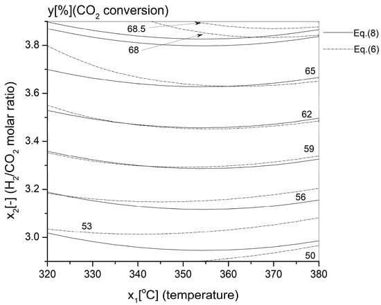
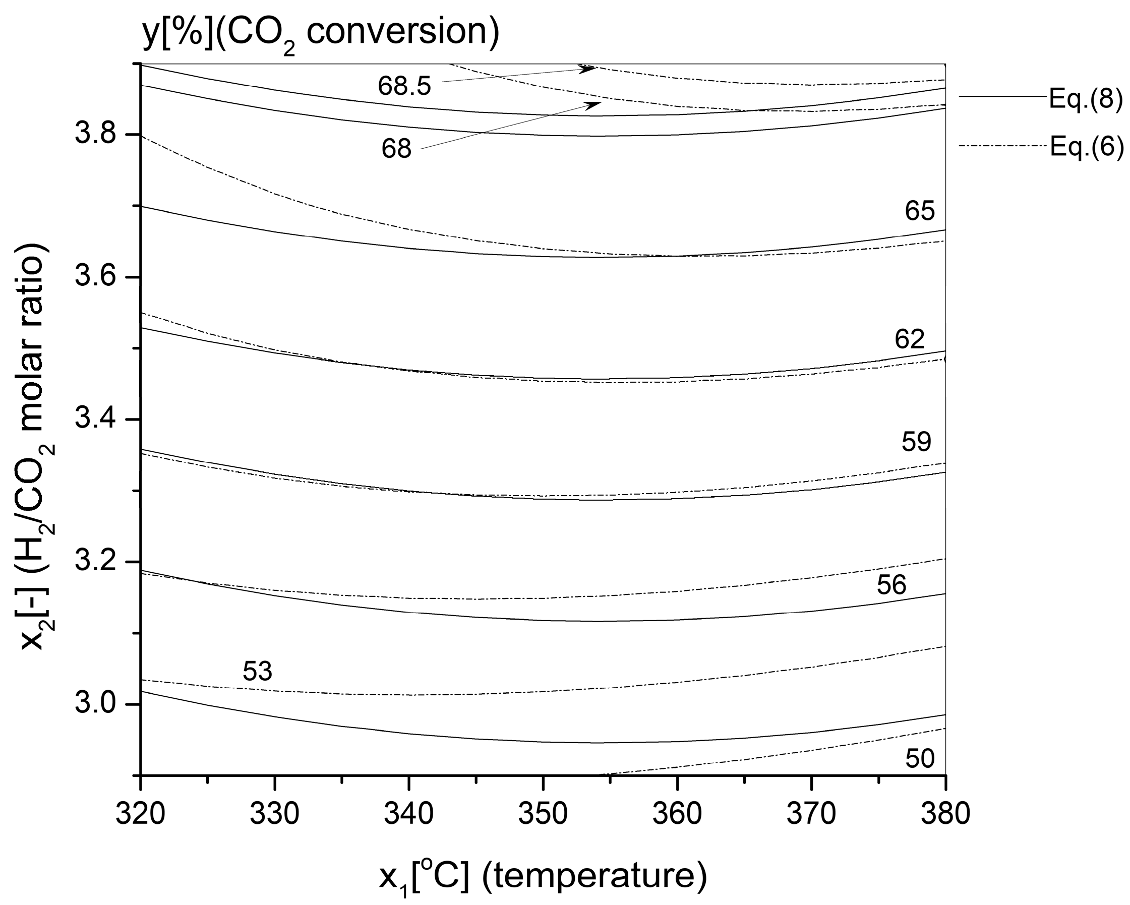
This discrepancy was experimentally verified. The conversion of carbon dioxide conversion at x₁ = 354 °C and x₂ = 3.9 is equal to 70.0%, which means that the result predicted by Model (8) is practically error-free. In contrast to this result, Model (6) does not anticipate as high of a conversion at a temperature of 354 °C. The result of this experiment confirms the result of the simulation, and so the model can be used to determine operating condition in the real process. Let us look closely at this issue. Figure 2 presents a contour plot of the response surface for both models.

Figure 2. Contour plot for the second-order models.

In general, the contours show that the models’ predictions for the same concentration ratio are similar, but there appears to be a clear temperature offset, so the determination of the better model plays the primary role. The rating must be based on experimental results, not on statistical indicators. Table 6 presents the results.

Table 6. Additional experimental verification of the accuracy of the models.

x1 [°C]	x2 [-]	yeq(6) [%]	yeq(8) [%]	yexp [%]
290	3.2	53.6	53.0	52.4
332	2.9	50.3	51.6	52.4
360	2.8	46.9	50.3	49.2
372	2.7	42.7	48.1	47.2

The experiments carried out show Model (8) has a clear advantage. The difference between the experiment and the prediction is always smaller. As a consequence, Model (8) is superior, and the presence of statistically insignificant coefficients in Model (6) worsens the precision of the predictions and can even produce large errors, such as a shift in optimal temperature for Model (6).

4. Conclusions

The goal of this work was realized with a successful result. Similarly to investigations with a laboratory-scale reactor [1], the choice of a statistical method that supports the experiments was prudent. The RSM and CCD reduced the number of experiments required to determine the optimal operating conditions. Furthermore, the RSM involves simple mathematical models of the empirical type. However, here, finding the optimal conditions was not as simple as presented in [1]. The larger scale of the process caused some trouble. The first model developed included coefficients that were statistically insignificant; for this reason, another model was developed, and additional experiments were necessary to compare goodness of the models. The investigations carried out show, without a doubt, that Model (8) is more precise than Model (6). Next, inside the investigated region, neither model has a maximum, and optimal conditions were found to be an extreme value of the function that describes the considered process. The experiments confirm the results calculated using Model (8). Despite the difficulties presented, the RSM can be recommended as a tool that supports experimentation and substantially speeds up analysis and the introduction of results into practice.

References

- Szukiewicz, M.K.; Patulska, N.; Chmiel-Szukiewicz, E. A Fast and Efficient Response Surface Approach for the Optimization of the Gas-Phase Hydrogenation of Carbon Dioxide on Nickel-Based Catalysts. Reactions 2025, 6, 16. [Google Scholar] [CrossRef] [Scilit]
- Montgomery, D.C. Design and Analysis of Experiments, 9th ed.; Wiley: Hoboken, NJ, USA, 2017. [Google Scholar]
- Myers, R.H.; Montgomery, D.C.; Anderson-Cook, C.M. Response Surface Methodology: Process and Product Optimization Using Designed Experiments, 4th ed.; Wiley: Hoboken, NJ, USA, 2016. [Google Scholar]
- Ridzuan, N.D.M.; Shaharun, M.S.; Anawar, M.A.; Ud-Din, I. Ni-Based Catalyst for Carbon Dioxide Methanation: A Review on Performance and Progress. Catalysts 2022, 12, 469. [Google Scholar] [CrossRef] [Scilit]
- Stangeland, K.; Kalai, D.; Li, H.; Yu, Z. CO2 Methanation: The effect of catalysts and reaction conditions. Energy Procedia 2017, 105, 2022–2027. [Google Scholar] [CrossRef] [Scilit]
- Aziz, M.A.A.; Jalil, A.A.; Triwahyono, S.; Ahmad, A. CO2 methanation over heterogeneous catalysts: Recent progress and future prospects. Green Chem. 2015, 17, 2647–2663. [Google Scholar] [CrossRef] [Scilit]
- Gao, J.; Liu, Q.; Gu, F.; Liu, B.; Zhong, Z.; Su, F. Recent advances in methanation catalysts for the production of synthetic natural gas. RSC Adv. 2015, 5, 22759–22776. [Google Scholar] [CrossRef] [Scilit]
- Li, Y.; Chan, S.H.; Sun, Q. Heterogeneous catalytic conversion of CO2: A comprehensive theoretical review. Nanoscale 2015, 7, 8663–8683. [Google Scholar] [CrossRef] [Scilit] [PubMed]
- Gao, J.; Wang, Y.; Ping, Y.; Hu, D.; Xu, G.; Gu, F.; Su, F. A thermodynamic analysis of methanation reactions of carbon oxides for the production of synthetic natural gas. RSC Adv. 2012, 2, 2358–2368. [Google Scholar] [CrossRef] [Scilit]
- Hayes, R.E.; Thomas, W.J.; Hayes, K.E. A study of the nickel-catalyzed methanation reaction. J. Catal. 1985, 92, 312–326. [Google Scholar] [CrossRef] [Scilit]
- Chiang, J.H.; Hopper, J.R. Kinetics of the hydrogenation of carbon dioxide over supported nickel. Ind. Eng. Chem. Prod. Res. Dev. 1983, 22, 225–228. [Google Scholar] [CrossRef] [Scilit]
- Jalama, K. Carbon dioxide hydrogenation over nickel-, ruthenium-, and copper-based catalysts: Review of kinetics and mechanism. Catal. Rev. 2017, 59, 95–164. [Google Scholar] [CrossRef] [Scilit]
- Ioelovich, M. Thermodynamic analysis of methane synthesis by hydrogenation of carbon dioxide. World J. Adv. Res. Rev. 2024, 24, 927–931. [Google Scholar] [CrossRef] [Scilit]
Disclaimer/Publisher’s Note: The statements, opinions and data contained in all publications are solely those of the individual author(s) and contributor(s) and not of MDPI and/or the editor(s). MDPI and/or the editor(s) disclaim responsibility for any injury to people or property resulting from any ideas, methods, instructions or products referred to in the content. |
© 2026 by the authors. Licensee MDPI, Basel, Switzerland. This article is an open access article distributed under the terms and conditions of the Creative Commons Attribution (CC BY) license.