


Abstract
Accurate estimation of winter wheat canopy nitrogen concentration (CNC) supports crop diagnosis and precision nitrogen management, yet the relative value and redundancy of multispectral, structural, and chlorophyll-related variables remain unclear in small dat asets. Using 155 multi-temporal observations retained from the 2016–2017 and 2017–2018 growing seasons, seven prespecified feature combinations were evaluated with four traditional regression models under five-fold repeated season-stratified cross-validation. A stricter season-balanced, unit-level grouped five-fold cross-validation was added to prevent observations from the same field from occurring in both training and test partitions. Two fully connected neural networks were additionally assessed for the selected compact module. Spectral-only combinations yielded negative mean R2 values, whereas LAI, vegetation cover, and chlorophyll content achieved a mean R2 of 0.684. Combining these variables with four raw multispectral bands produced M5, which achieved mean RMSE, R2, and RPD values of 0.328, 0.782, and 2.147, respectively, with 36.4% fewer variables than the full module. RF provided the best numerical performance under repeated sample-level cross-validation (R2 = 0.796 ± 0.007), whereas M5 retained R2 values of 0.736–0.778 under unit-grouped validation, with SVR performing best in that stricter setting. Parameter-removal analysis showed the largest incremental contribution for vegetation cover and limited additional value from LAI. Bidirectional cross-season validation remained direction- and model-dependent. Overall, controlled low-redundancy feature fusion was more beneficial than increased model complexity, while field-level and cross-season tests indicated that the strong within-dataset results should not be interpreted as broad generalization capability.
1. Introduction
Nitrogen is a key nutrient affecting winter wheat growth, yield formation, grain quality, and fertilizer-use efficiency. Accurate estimation of winter wheat nitrogen status is therefore useful for precision fertilization and field diagnosis [1,2,3,4]. Conventional laboratory analysis is accurate but time-consuming, costly, and spatially discontinuous, which limits rapid field-scale assessment [1,4]. Unmanned aerial vehicle (UAV) multispectral remote sensing provides high spatial resolution, flexible acquisition windows, and repeatable observation, and has been widely used for crop growth monitoring and nitrogen diagnosis [5,6,7]. Red, red-edge, and near-infrared bands, together with vegetation indices such as the normalized difference vegetation index (NDVI), normalized difference red-edge index (NDRE), modified chlorophyll absorption ratio index (MCARI), and red-edge chlorophyll index (CIre), are commonly used to retrieve chlorophyll- and nitrogen-related crop traits [8,9,10]. Nevertheless, spectral signals represent the combined effects of pigments, canopy structure, soil background, illumination, viewing geometry, and crop development stage rather than nitrogen concentration alone. Consequently, similar CNC values can be associated with different canopy structures, and similar spectral responses can arise from different combinations of nitrogen status, chlorophyll absorption, leaf overlap, and canopy coverage.
The prediction target used in this study should be distinguished from other commonly reported crop nitrogen indicators. In the public dataset, N_concentration_wheat denotes the mass-based nitrogen concentration of above-ground wheat material, expressed as a percentage of dry weight; it is referred to here as canopy nitrogen concentration (CNC). Unlike nitrogen uptake or canopy nitrogen content per unit ground area, CNC is not multiplied by biomass, and it also differs from the nitrogen nutrition index (NNI), which expresses actual nitrogen status relative to a critical nitrogen-dilution reference [2,3,4,11,12,13]. Thus, the CNC values reported in this study should not be interpreted as nitrogen uptake or NNI. Unlike previous studies that primarily aimed to maximize prediction accuracy through heterogeneous multisource feature fusion or model optimization, the present study focuses on isolating the incremental contribution and redundancy of predefined feature groups under identical validation and modeling conditions.
Canopy structural and chlorophyll-related parameters can provide complementary information. Leaf area index (LAI) and fraction of vegetation cover (fCover) characterize canopy size and coverage, whereas chlorophyll content (CC) reflects leaf chlorophyll status [14,15,16]. Recent wheat nitrogen studies have combined UAV spectral information with structural, textural, meteorological, management, RGB, or thermal variables and machine-learning models [17,18,19,20]. For example, Jiang et al. [17] integrated multispectral, agrometeorological, and management information for NNI estimation across multiple field experiments, while Zhang et al. [18,19] investigated higher-dimensional spectral–texture or multisensor feature sets and transfer strategies across contrasting management, location, cultivar, and growth-stage conditions. These studies demonstrate the value of multisource fusion, but differences in prediction target, feature space, growth-stage coverage, and validation design make direct performance comparison difficult.
Moreover, many previous studies optimize heterogeneous feature sets and algorithms simultaneously, so the independent and incremental value of individual information groups remains difficult to separate. This issue is especially important for small datasets, where additional predictors and model complexity can increase redundancy and selection uncertainty. Traditional linear, kernel-based, and tree-ensemble models may remain competitive under low-dimensional small-sample conditions, whereas neural-network complexity should be tested rather than assumed to improve prediction. A controlled comparison using identical data partitions and prespecified model settings is therefore useful for distinguishing gains attributable to input information from those attributable to algorithm choice.
Accordingly, this study used the public in situ and UAV winter wheat dataset [21,22] as a controlled small-sample benchmark. Specifically, we (1) compared seven prespecified combinations of raw multispectral bands, vegetation indices, LAI, fCover, and CC under identical data partitions and fixed traditional-model settings; (2) quantified redundancy and incremental information using correlation analysis, VIFs, paired repetition-level comparisons, and parameter-removal experiments; (3) compared traditional regressors with shallow and deeper fully connected neural networks under the same repeated cross-validation framework, while treating the neural networks only as model-complexity comparators; and (4) evaluated robustness using both unit-level grouped cross-validation and exploratory bidirectional cross-season transfer without overstating generalizability.
The contribution is therefore a controlled multisource feature-modeling benchmark for small-sample CNC estimation rather than a new sensor, neural-network architecture, or complete end-to-end UAV nitrogen-management system. Because LAI, fCover, and CC were measured by the dataset providers rather than retrieved from UAV imagery, the results should be interpreted as an evaluation of information contribution and robustness under the available multisource dataset.
2. Materials and Methods
2.1. Public Dataset and Study Area
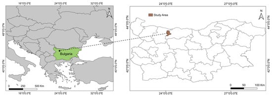
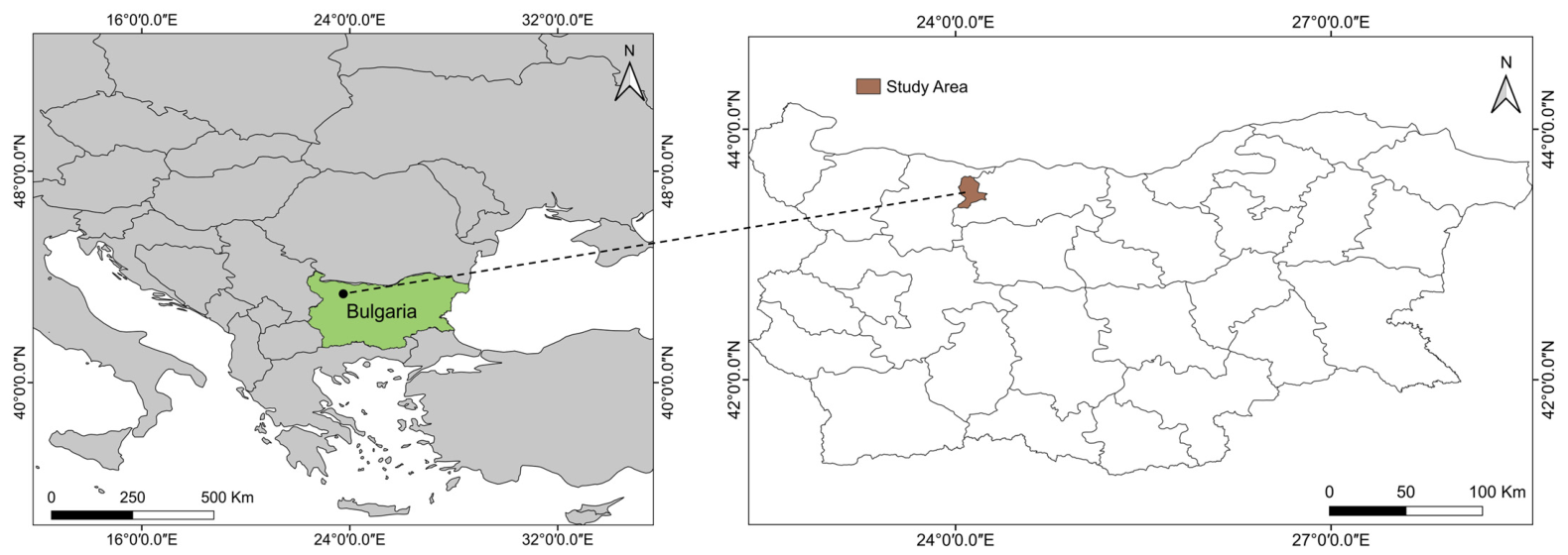
This study used the publicly released dataset entitled “In-situ and UAV dataset with crop and soil parameters obtained from winter wheat fields”. The dataset is available from Zenodo (DOI: 10.5281/zenodo.17475742) and is described by Dimitrov et al. [21,22]. The dataset was produced under the European Space Agency-funded TS2AgroBg project. As shown in Figure 1, the observation area was located in the Zlatia agricultural test site near Knezha on the Danube Plain in northern Bulgaria. The archive covers the 2016–2017 and 2017–2018 agricultural seasons and contains ESU-scale biophysical and biochemical measurements, field spectral data, phenology and soil data, crop-management records, unit and ESU shapefiles, meteorological data, and campaign-specific four-band UAV mosaics [21,22].
Figure 1.
Location of the study area in northern Bulgaria.
No new field sampling was conducted. The original design followed a hierarchical unit–ESU–ESSU framework. A unit represents one commercial agricultural field, an elementary sampling unit (ESU) is a 20 m × 20 m plot, and three elementary sub-sampling units (ESSUs) were used for repeated measurements within each ESU; the released tabular values are averaged at the ESU scale [22]. Six units were sampled in each agricultural season, and ESU locations were generally revisited across campaigns within the same season. The dataset uses Unit_ID values such as S16-17_U1 and ESU_ID values such as apr2017_1_2, where the latter encodes campaign month/year, unit number, and ESU number. This hierarchy was retained explicitly in the revised validation design.
2.2. Data Screening and Definition of the Target Variable
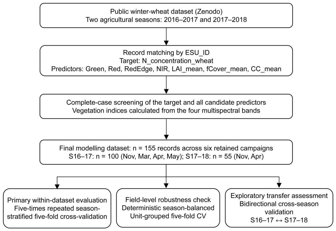
N_concentration_wheat was used as the prediction target [21,22]. According to the dataset documentation, this variable is the nitrogen concentration of above-ground wheat organs expressed as a percentage of dry weight; it is referred to here as CNC. The modeling table was constructed at the ESU-record level using ESU_ID as the temporal–spatial key. The required measured variables were N_concentration_wheat, LAI_mean, fCover_mean, and CC_mean, and the four spectral predictors were Green, Red, RedEdge, and NIR values corresponding to the Sequoia UAV bands. The public archive components relevant to this construction include ESU_Biophysical_and_biochemical_crop_data.txt, Shapefile_ESUs.zip, Shapefile_Units.zip, and the campaign-specific UAV mosaic archives [21,22]. Records were retained only when the target and all 11 candidate predictors required for the full M7 feature set were available; no filtering was performed on the basis of CNC magnitude or model performance. Complete-case matching yielded 155 records from six retained campaigns: 100 records from the 2016–2017 season and 55 from the 2017–2018 season (Table 1). The same ESU could appear in more than one campaign as a distinct temporal record.
Table 1.
Composition of the 155 retained multi-temporal observations after complete-case matching.
2.3. Feature Construction
The UAV mosaics were acquired by the dataset providers using an eBee Ag fixed-wing platform (EagleNXT, Wichita, KS, USA; formerly senseFly, Cheseaux-Lausanne, Switzerland) equipped with a Sequoia multispectral camera (Parrot Drones SAS, Paris, France) [21,22]. The sensor records green (550 nm), red (660 nm), red-edge (735 nm), and near-infrared (790 nm) bands; the nominal bandwidth is 40 nm except for the 10 nm red-edge band. UAV mosaics were generated for each retained campaign. The November 2016 campaign used a flight height of approximately 106 m with 75% forward and side overlap, producing approximately 10 cm ground resolution; subsequent campaigns used approximately 265 m with 80% overlap and approximately 25 cm ground resolution [22]. Flights were conducted between 10:00 and 14:00 local time. Ground control points measured with a Leica GS08+ GNSS receiver (Leica Geosystems AG, Heerbrugg, Switzerland) were used to refine georeferencing, and Pix4Dmapper (Pix4D S.A., Prilly, Switzerland; version not reported in the source documentation) was used by the dataset providers for irradiance-based radiometric processing, orthorectification, and mosaicking. Radiometric processing converted image values to surface reflectance using irradiance measurements from the Sequoia sunshine sensor [22]. The present modeling analysis used the aligned ESU-level four-band values and did not reprocess the original UAV mosaics.
Four vegetation indices were calculated from the released band reflectance values: normalized difference vegetation index (NDVI), normalized difference red-edge index (NDRE), modified chlorophyll absorption ratio index (MCARI), and red-edge chlorophyll index (CIre) [8,9,10]. LAI_mean, fCover_mean, and CC_mean were selected as the biophysical and chlorophyll-related variables and are hereafter denoted LAI, fCover, and CC. LAI and fCover were measured by the dataset providers with an AccuPAR LP-80 ceptometer (METER Group, Inc., Pullman, WA, USA; formerly Decagon Devices, Inc., Pullman, WA, USA), while CC was measured with a CCM-300 chlorophyll content meter (Opti-Sciences, Inc., Hudson, NH, USA) [22]. The released values were averaged at the ESU scale. LAI, fCover, and CC were not estimated from the UAV imagery in this study. Therefore, the analysis should be interpreted as a controlled evaluation of multispectral and measured biophysical feature combinations. The results describe the information contribution of the evaluated variables and do not constitute a complete image-to-CNC operational workflow.
2.4. Feature-Combination Design
Seven prespecified feature combinations were constructed as controlled contrasts (Table 2). M1 and M2 independently represented the two basic forms of spectral information, namely the four original multispectral bands and four derived vegetation indices, respectively. M3 combined these two spectral representations to examine whether the derived indices provided complementary information beyond the original bands. M4 consisted only of LAI, fCover, and CC and was used as a biophysical/chlorophyll-related reference combination without spectral predictors. M5 and M6 were then constructed by adding either the four raw bands or the four vegetation indices to M4. Because both combinations contained seven variables and shared the same three measured biophysical/chlorophyll-related predictors, their comparison provided a controlled assessment of whether raw spectral measurements or derived indices contributed more useful incremental information.
Table 2.
Composition of the seven prespecified feature combinations and their corresponding controlled comparisons.
M7 included all 11 candidate variables and represented the complete feature set. Comparison of M5 with M7 was particularly important for evaluating whether adding vegetation indices to an already fused raw-band and biophysical feature set improved prediction sufficiently to justify the additional dimensionality and redundancy. All seven combinations were defined before model evaluation and were assessed using identical data partitions and model settings so that differences in predictive performance could be attributed primarily to feature composition rather than to changes in the modeling protocol.
2.5. Regression Models
Partial least squares regression (PLSR), support vector regression (SVR), random forest (RF), and extreme gradient boosting (XGBoost) were used as representative linear latent-variable, kernel-based, bagging-ensemble, and boosting-ensemble regressors [23,24,25,26]. To examine whether increasing neural-network complexity was beneficial under the present small-sample and low-dimensional conditions, a shallow multilayer perceptron (MLP) and a deeper fully connected neural network (FCNN) were evaluated under M5. The neural networks were included as comparison models rather than proposed architectures. All hyperparameters were specified a priori from the preliminary experimental design and commonly used settings; no grid, random, or Bayesian search was performed. This choice was deliberate: using fixed settings gave every feature combination the same modeling budget, reduced additional selection on a small dataset, and kept the main comparison focused on input information rather than model-specific optimization. Consequently, the reported values represent performance under prespecified configurations rather than the theoretical optimum of each algorithm. SiLU activation [27], dropout regularization [28], the Adam optimizer [29], and mean squared error (MSE) loss were used for the neural networks. MLP used fully connected layers of 7-16-32-16-1 with dropout of 0.20, whereas the FCNN used 7-32-32-16-8-1 with dropout of 0.25. For both networks, batch size was 16, learning rate was 1 × 10⁻⁴, L2 weight decay was 1 × 10⁻⁴, maximum training length was 1000 epochs, and early-stopping patience was 100 epochs based on validation RMSE. Network initialization and data-loader shuffling were controlled by deterministic fold-specific random seeds. The traditional-model and neural-network settings are summarized in Table 3.
Table 3.
Prespecified hyperparameter settings for the six regression models used in the comparative evaluation.
2.6. Repeated Cross-Validation and Model Evaluation
Five-bin stratification based on CNC values was removed from the final analysis. Instead, the primary evaluation used five repetitions of five-fold cross-validation stratified only by growing-season membership. This strategy preserved the proportional representation of the 100 S16–17 and 55 S17–18 records across folds while avoiding additional response-value-based constraints on fold construction. The same outer folds were used for every feature combination and model. For each outer split, one fold was kept untouched for testing, and the other four folds were used for model training. Standardization was fitted only on the outer training data. For MLP and FCNN, 20% of the outer training data were internally reserved for epoch selection. Training used MSE loss, and early stopping was triggered when validation RMSE failed to improve for 100 consecutive epochs. The selected epoch number was then used to retrain the network from scratch on the complete outer training fold before evaluation on the untouched outer test fold. No additional hyperparameter optimization or test-set feedback was used.
Model performance was evaluated using root mean square error (RMSE), coefficient of determination (R2), and ratio of performance to deviation (RPD) [30]. RMSE quantifies prediction error, R2 describes explained variation, and RPD is the ratio of the standard deviation of observed test values to RMSE. Lower RMSE and higher R2 and RPD indicate better performance. The metrics were calculated using Equations (5)–(7).
where n is the number of validation samples, yi is the measured CNC value of the i-th sample, is the corresponding predicted value, is the mean of the measured CNC values, and SD is the standard deviation of the measured CNC values in the validation set. Prediction bias was additionally reported in the model-comparison table to describe systematic over- or under-prediction.
For each repetition, the five outer-fold predictions were pooled to generate a complete out-of-fold prediction vector. Metrics were calculated from each pooled vector and are reported as mean ± standard deviation across the five repetitions; these repetition-level metrics are the primary performance estimates for the repeated-CV analysis. Feature-combination contrasts were assessed using paired repetition-level differences and bootstrap 95% confidence intervals. Because only five repetitions were available, the paired uncertainty analyses were treated as supportive rather than definitive and were not used to claim statistical equivalence or universal superiority.
2.7. Season-Balanced, Unit-Level Grouped Cross-Validation
To evaluate the possibility that observations from the same field could inflate sample-level cross-validation performance, an additional unit-level grouped five-fold cross-validation was performed. Unit_ID was defined according to the dataset convention as the combination of agricultural season and unit number (e.g., S16-17_U4), yielding 12 season-specific field groups. All temporal records and ESUs belonging to a unit were assigned together to either training or testing, so no unit was shared between the two partitions in any fold. Because only six units were available per season, a single deterministic season-balanced partition was predefined rather than repeatedly resampling a small number of groups. Within each season, whole units were ordered by sample count and assigned to folds to balance sample numbers while ensuring that every test fold contained observations from both seasons. No CNC-based stratification was applied in the unit-level grouped analysis; neither CNC values nor CNC quantile bins were used for fold construction. Instead, fold assignment prioritized complete unit separation and approximate season balance. The resulting five test folds contained 29–34 records and two or four complete units, with zero train–test unit overlap. The same grouped folds were used for M1–M7 with PLSR, SVR, RF, and XGBoost. MLP and FCNN were not repeated in this robustness analysis because they were auxiliary complexity comparators evaluated only under M5, whereas the grouped analysis was designed to reproduce the complete M1–M7 feature-combination experiment under a stricter field-independent partition. Primary grouped-CV metrics were calculated from the pooled out-of-fold predictions across all five folds; fold-level metrics were used only as descriptive diagnostics. The same predefined unit-level fold assignment was used for all feature combinations and models in this robustness analysis.
2.8. Redundancy, Parameter-Contribution, and Cross-Season Validation
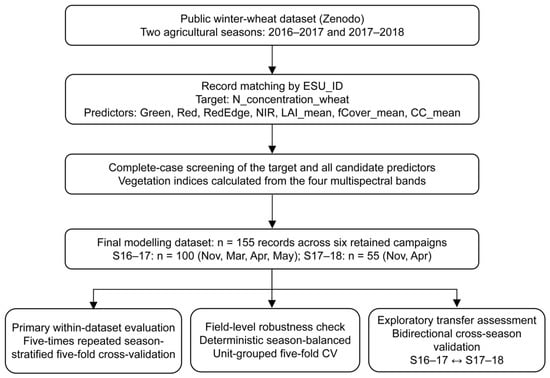
To characterize predictor redundancy, Pearson correlation coefficients were first used to describe bivariate relationships, and variance inflation factors (VIFs) were calculated for predictors in the compact M5 and full M7 combinations. For each predictor, VIF was computed as VIF = 1/(1 − R2), where R2 is the coefficient of determination obtained by regressing that predictor on all remaining predictors within the same feature combination. VIFs were calculated using the pooled 155-record dataset and were treated as descriptive diagnostics of linear redundancy. After the seven prespecified modules had been evaluated, parameter-contribution experiments removed LAI, fCover, or CC one at a time and compared the resulting performance with M1 and M4. These removal tests were post hoc and were interpreted as diagnostics of incremental contribution rather than as measures of intrinsic feature importance. To characterize between-season differences relevant to model transfer, CNC distributions in S16–17 and S17–18 were summarized separately and compared using Welch’s t-test and the two-sample Kolmogorov–Smirnov (KS) test. Season-specific Pearson correlations between CNC and the seven M5 variables were also calculated. Exploratory bidirectional cross-season validation trained models on all 100 S16–17 observations and evaluated them on the 55 S17–18 observations, and vice versa. M4, M5, and M7 were evaluated with the four traditional models using the same fixed parameter settings, with scaling and model fitting performed using the training season only. Because the two seasons differed in training size, retained campaign composition, fields, target distribution, and some feature–target relationships, these tests were intended to characterize transfer sensitivity rather than isolate a pure year effect or claim independent external validation. The overall data-construction and validation workflow is summarized in Figure 2.
Figure 2.
Construction of the 155-record modeling dataset and the three complementary validation strategies used in this study. Arrows indicate the sequence of data processing and the branching into the three validation strategies.
3. Results
3.1. Correlation, Multicollinearity, and Feature-Combination Results
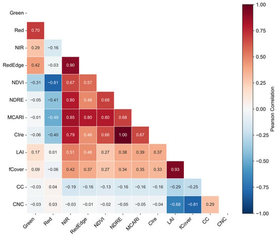
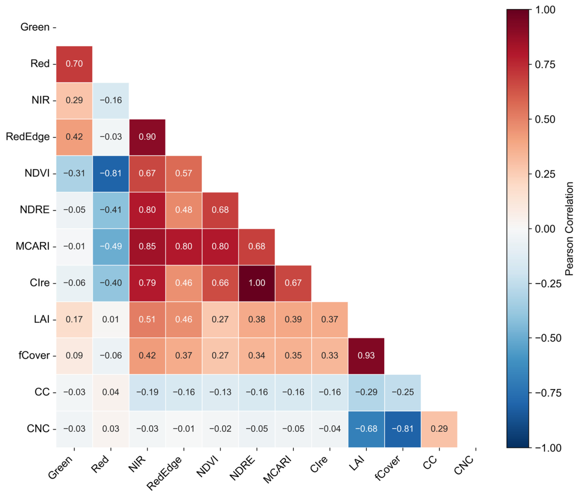
The correlation matrix is shown in Figure 3. CNC was weakly correlated with the four raw bands and four vegetation indices (|r| ≤ 0.05), but showed stronger relationships with LAI (r = −0.68), fCover (r = −0.81), and CC (r = 0.29). LAI and fCover were highly correlated with each other (r = 0.93), indicating that their information was not independent. To further quantify the predictor redundancy suggested by the correlation matrix, VIFs were examined for the compact M5 and full M7 combinations. In M5, VIF values ranged from 1.10 for CC to 8.93 for LAI, while fCover also showed a relatively high VIF of 7.79, consistent with the strong correlation between LAI and fCover. In contrast, M7 showed severe multicollinearity, with VIF values exceeding 200 for Red, RedEdge, NIR, NDVI, NDRE, and CIre; the maximum VIF was 513.07 for RedEdge. These results indicate that adding vegetation indices to the original bands substantially increased predictor redundancy.
Figure 3.
Pearson correlation matrix among the candidate input variables and canopy nitrogen concentration (CNC).
The model-specific repeated-CV R2 results for the seven prespecified feature combinations are summarized in Table 4 as mean ± SD across five repetitions. The three spectral-only combinations M1–M3 produced negative mean R2 values for all four traditional models, indicating that spectral variables alone did not provide stable CNC predictions in this dataset. M4, which contained only LAI, fCover, and CC, achieved mean R2 values of 0.676–0.692. Adding the four raw bands to form M5 increased mean R2 to 0.769–0.796 across the four models. M6 was less accurate than M5, while M7 yielded mean R2 values of 0.759–0.797. Paired repetition-level comparisons supported the incremental value of raw bands: the bootstrap 95% confidence intervals for the M4-to-M5 RMSE change excluded zero for all four traditional models. By contrast, adding the four vegetation indices to M5 did not produce a consistent repeated-CV benefit. For M7 relative to M5, the mean paired ΔRMSE values (M7 − M5) were 0.0073 (95% CI: 0.0050–0.0113) for PLSR, 0.0004 (−0.0037–0.0044) for SVR, −0.0011 (−0.0025–0.0009) for RF, and 0.0023 (−0.0018–0.0064) for XGBoost. Thus, PLSR showed a deterioration, whereas the differences for SVR, RF, and XGBoost were small and their confidence intervals included zero. M5 was therefore treated as the preferred compact combination under the present pooled protocol, rather than as a universally optimal feature set: it used seven variables instead of eleven, reduced dimensionality by 36.4%, avoided the extreme band-index multicollinearity of M7, and achieved comparable or better mean performance.
Table 4.
Five-fold repeated season-stratified cross-validation R2 for the seven feature combinations. Values are mean ± SD across five repetitions.
3.2. Unit-Level Grouped Cross-Validation
The stricter unit-level grouped evaluation preserved the main feature-combination pattern (Table 5). Spectral-only M1–M3 remained unstable, with pooled R2 values near or below zero. M4 yielded R2 = 0.616–0.677, whereas M5 retained R2 = 0.736–0.778 across the four traditional models. Relative to the primary repeated sample-level evaluation, the M5 R2 change was −0.017 for PLSR, −0.002 for SVR, −0.060 for RF, and −0.045 for XGBoost. Thus, the linear/kernel models were comparatively stable, while the tree ensembles showed a larger reduction after field-level separation. M5 also remained competitive with M7: M5 was higher for PLSR and SVR, whereas M7 exceeded M5 by only 0.007 for RF and 0.002 for XGBoost. The grouped analysis therefore supports M5 as a parsimonious configuration under a field-independent partition, while also showing that the model ranking was not invariant: SVR, rather than RF, achieved the highest grouped-CV R2 (0.778).
Table 5.
Season-balanced, unit-level grouped five-fold cross-validation for M1–M7. Each model cell reports pooled out-of-fold RMSE/R2 across all five grouped folds.
3.3. Model Comparison and Parameter Contribution Under M5
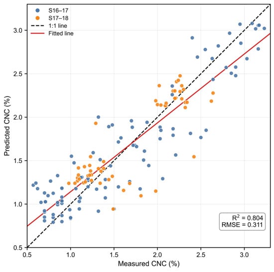
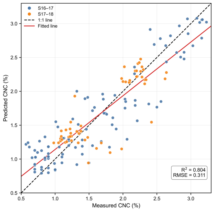
Table 6 compares the six models under M5 using the primary repeated-CV protocol. RF achieved the lowest numerical RMSE (0.318 ± 0.006) and the highest R2 (0.796 ± 0.007) and RPD (2.215 ± 0.040), followed by XGBoost, SVR, and PLSR. MLP and FCNN achieved lower accuracy than all four traditional models. The decline from MLP to the deeper FCNN indicates that increasing network depth did not provide an advantage for the present dataset of 155 low-dimensional tabular records. This comparison is intentionally limited to prespecified settings and should not be interpreted as proof that RF is universally superior. Indeed, the added unit-grouped analysis changed the numerical ranking under M5, with SVR giving the highest field-grouped R2. Together, the two validation schemes indicate that model ranking is sensitive to partition structure. Figure 4 visualizes the sample-level mean out-of-fold predictions of the M5-RF model. After averaging each sample’s out-of-fold prediction across the five repetitions, the resulting vector yielded R2 = 0.804 and RMSE = 0.311 (n = 155). These values are not the primary performance estimate and should not be compared directly with a single repetition. Table 6 reports metrics calculated separately for each complete repetition and then summarized as mean ± SD.
Table 6.
Repeated season-stratified cross-validation performance of the six regression models under M5. Values are mean ± SD across five repetitions; these are the primary repeated-CV performance estimates.
Figure 4.
Measured versus predicted canopy nitrogen concentration (CNC) for the RF model under M5. Each point represents the mean out-of-fold prediction for an individual sample across five repeated cross-validations. This sample-averaged visualization is descriptive; the primary performance estimates are the repetition-level mean ± SD values in Table 6.
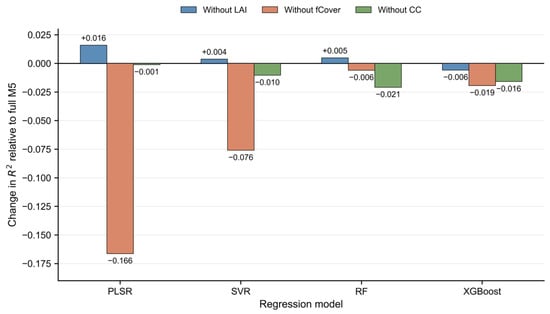
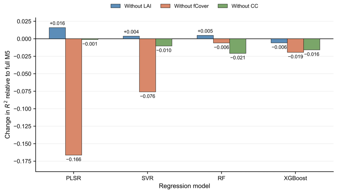
The parameter-removal results are summarized in Table 7 and Figure 5. Averaged across the four traditional models, removing fCover reduced mean R2 from 0.782 to 0.716, the largest performance loss among the three one-variable removal tests. The effect was model-dependent: the R2 reduction was greatest for PLSR (ΔR2 = −0.166) and SVR (ΔR2 = −0.076), but small for RF (ΔR2 = −0.006). Removing CC produced smaller negative changes (ΔR2 = −0.001 to −0.021). Removing LAI slightly improved R2 for PLSR, SVR, and RF (+0.016, +0.004, and +0.005), whereas XGBoost decreased slightly (−0.006). This pattern is consistent with the strong LAI–fCover correlation and indicates limited incremental information from LAI once fCover and the spectral bands are present; it does not imply that LAI is intrinsically unimportant. Because the removal analysis was conducted after the seven prespecified modules had been evaluated, it is interpreted only as a post hoc simplification diagnostic.
Table 7.
Model-specific repeated-CV R2 under full M5 and after removing LAI, fCover, or CC. Values are means across five repetitions.
Figure 5.
Changes in mean R2 relative to the full M5 feature combination after removing LAI, fCover, or CC for each traditional regression model. Positive values indicate improved performance, whereas negative values indicate performance loss.
3.4. Exploratory Cross-Season Validation
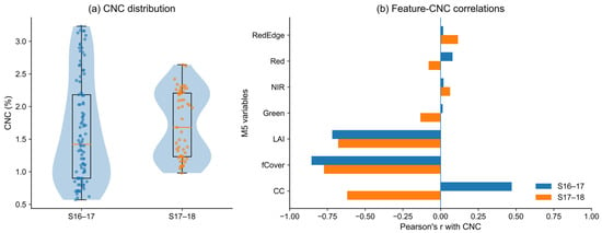
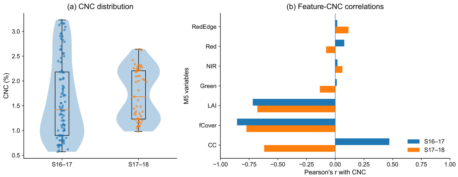
To characterize between-season differences relevant to model transfer, Table 8 and Figure 6 summarize CNC distributions and season-specific feature–CNC relationships. Mean CNC was 1.620% in S16–17 and 1.725% in S17–18. Welch’s t-test showed no significant difference between the two means (t = −1.004, p = 0.317; Table 8). However, S16–17 covered a substantially broader CNC range (0.570–3.230%) than S17–18 (0.980–2.640%), and the two-sample KS test confirmed a difference in the overall distributions (D = 0.312, p = 0.001). Figure 6b shows that the CNC relationships with LAI (r = −0.72 and −0.68 for S16–17 and S17–18) and fCover (r = −0.86 and −0.77) were relatively stable in direction, whereas the CC–CNC association changed from positive in S16–17 (r = 0.47) to negative in S17–18 (r = −0.62). These contrasts should be interpreted as season-specific descriptive differences because the retained campaign composition also differed between the two seasons.
Table 8.
Descriptive statistics and between-season comparison of canopy nitrogen concentration (CNC) in the 2016–2017 and 2017–2018 growing-season subsets.
Figure 6.
Between-season differences in CNC distribution and feature–CNC relationships. (a) CNC distributions in the 2016–2017 (S16–17) and 2017–2018 (S17–18) subsets; violin shapes show distribution density, internal boxplots indicate the median and interquartile range, and points represent individual records. (b) Season-specific Pearson correlations between CNC and the seven variables included in M5. Statistical comparisons of the CNC distributions are reported in Table 8.
Against this background, the exploratory cross-season validation results were strongly dependent on transfer direction, feature combination, and algorithm (Table 9). When models were trained on S16–17 and tested on S17–18, the best result was obtained by M7-PLSR (RMSE = 0.276; R2 = 0.700), whereas M5 achieved R2 values of 0.433 with PLSR and 0.513 with SVR. In the reverse direction, M5-PLSR obtained the best result (RMSE = 0.489; R2 = 0.618), while M7-PLSR achieved R2 = 0.551. Several RF and XGBoost transfers had low or negative R2 values. The directional asymmetry cannot be attributed to a single cause: the training sizes differed (100 versus 55 records), S16–17 contained four retained campaigns whereas S17–18 contained two, the target distributions and some feature–target relationships differed, and the season-specific units were not identical fields. These results show that strong within-dataset performance did not translate into uniformly robust cross-season transfer.
Table 9.
Exploratory bidirectional cross-season validation performance for M4, M5, and M7. Each model cell reports RMSE/R2; models were trained on one complete growing-season subset and evaluated on the other.
4. Discussion
4.1. Information Contributions of Spectral and Biophysical Variables
The spectral-only combinations performed poorly even though the study included red-edge and near-infrared information that is commonly associated with crop chlorophyll and nitrogen status. Across the retained multi-temporal campaigns, canopy reflectance was influenced simultaneously by pigment absorption, canopy cover, leaf overlap, soil background, illumination, geometry, and crop development stage. Weak direct spectral–CNC relationships therefore do not imply that the sensor bands contain no useful information; rather, their information was insufficient when used without structural and chlorophyll-related context. M4 confirmed that LAI, fCover, and CC contained substantial CNC-related information, and adding raw bands produced a further improvement. The removal tests showed the largest incremental performance contribution for fCover among the three measured variables. This is agronomically plausible because canopy expansion and biomass accumulation are linked to nitrogen dilution [11,12,13,14,15,16], but the interpretation remains indirect: above-ground biomass was not included as a predictor and no dilution curve was fitted. Moreover, because the pooled dataset spans several campaigns, part of the fCover contribution may reflect canopy-development and phenological differences among observation periods.
Direct comparison with recent studies requires caution because dataset composition, prediction targets, growth-stage coverage, predictor spaces, and validation strategies differ. Jiang et al. [17] used seven field experiments conducted over five years with different cultivars and nitrogen treatments to estimate NNI at the jointing and booting stages. Their RF model integrating UAV multispectral, agrometeorological, and field-management information achieved R2 values of 0.82–0.87, and the direct and indirect NNI diagnosis strategies were further evaluated across three study farms. Zhang et al. [18] estimated plant nitrogen content (PNC) using an eight-year long-term field experiment, with UAV and ground observations covering the returning-green, jointing, and grain-filling stages. By fusing UAV spectral and texture features, their best XGBoost model achieved R2 = 0.99; they also evaluated bidirectional model transfer between Farmers’ Practice and Ecological Intensification management systems, with transfer R2 values up to 0.98. Zhang et al. [19] used multi-location and multi-cultivar data across four growth stages to estimate NNI from UAV multispectral, RGB, and thermal information. Their dataset was further divided into six subsets according to location and cultivar to evaluate model transferability, and the best multisensor GPR model achieved R2 = 0.89 and RPD = 2.52. These studies therefore differ substantially from the present 155-record, two-season CNC dataset in prediction target, data scale, growth-stage coverage, predictor space, and validation design. Accordingly, their reported performance values should not be interpreted as directly comparable solely on the basis of R2. The present study instead emphasizes controlled information attribution and robustness under repeated, unit-grouped, and cross-season validation rather than maximizing an across-study R2 value.
4.2. Selecting a Compact Feature Combination
The comparison between M5 and M7 provides the main low-redundancy result. M7 added four vegetation indices but did not improve mean repeated-CV performance and created severe linear multicollinearity because the indices are deterministic transformations of the original bands. M5 retained similar predictive accuracy with 36.4% fewer variables and much lower VIFs. Importantly, high VIF does not imply that predictive information is necessarily lost, especially for tree-based models; it indicates linear redundancy and instability in attributing independent effects. This distinction is consistent with the results: under unit-grouped CV, RF and XGBoost performed almost identically with M5 and M7, whereas PLSR and SVR favored M5. Thus, the finding should not be generalized to vegetation indices as a class. It indicates only that NDVI, NDRE, MCARI, and CIre did not provide stable incremental value after the same raw bands and three measured biophysical variables were already present under this dataset, sensor, campaign composition, and modeling protocol. The post hoc LAI-removal result should be interpreted similarly. Because LAI and fCover were strongly correlated (r = 0.93), removing LAI slightly improved three models and slightly reduced one, indicating redundancy rather than evidence that LAI is agronomically unimportant. M5 was retained as the prespecified compact module; a six-variable variant should be tested only on independent data.
4.3. Model Complexity Under Small-Sample Conditions
RF provided the best numerical performance under the repeated sample-level protocol, whereas SVR performed best under the stricter unit-grouped protocol. This change in ranking reinforces the need to describe model superiority as conditional on validation design. MLP and FCNN did not outperform the traditional regressors under the repeated protocol. The input contained only seven tabular variables, and each outer training fold contained approximately 124 records before the internal neural-network validation split. The neural networks were trained with deterministic fold-specific initializations, MSE loss, and early stopping, and their reported variability reflects the five repeated outer partitions rather than a separate random-initialization benchmark. Under these conditions, additional network depth was not supported by the available data. The neural-network comparison is therefore best interpreted as a practical test of whether added model complexity helps in this small, low-dimensional setting, not as evidence against deep learning for UAV remote sensing. Deep models may be advantageous for image patches, dense spectra, multitemporal sequences, or substantially larger training sets [31,32,33,34,35].
4.4. Cross-Season Validation and Practical Interpretation
The exploratory bidirectional cross-season validation (Table 9) showed strong dependence on transfer direction. M7-PLSR performed best for S16–17 to S17–18, whereas M5-PLSR performed best in the reverse direction; several RF and XGBoost combinations showed low or negative transfer R2 despite strong repeated-CV performance. These results indicate that rankings from pooled within-dataset validation were not fully preserved across growing seasons. The descriptive summaries in Table 8 and Figure 6 provide context but do not identify a single causal mechanism. The S16–17 subset covered a broader CNC range, CC–CNC correlations changed in magnitude and sign, training sizes were unequal (100 versus 55), and the retained campaign composition differed substantially: S16–17 included November, March, April, and May records, whereas S17–18 included November and April. Consequently, the transfer contrast combines seasonal, phenological/campaign, field, and sample-size differences. It should therefore be interpreted as a stress test of cross-season transportability rather than as a controlled estimate of an isolated year effect.
The practical interpretation must also account for the data source. LAI, fCover, and CC were measured by the original dataset providers rather than retrieved from UAV imagery in the present study. M5 is therefore a compact multisource tabular configuration, not a directly deployable image-to-CNC pipeline. A future operational workflow would require UAV- or sensor-based retrieval of LAI, fCover, and CC, followed by CNC estimation using the fused predictors. Errors in those intermediate retrievals would propagate into the CNC model as covariate uncertainty; the present removal analysis suggests that fCover retrieval accuracy may be particularly important because its omission produced the largest average performance loss. Future studies should therefore quantify error propagation using independently validated retrieval models or error-in-variables/Monte Carlo perturbation analyses before operational use. Independent multi-site and multi-season evaluation is also required before claiming broad applicability [36,37,38,39,40,41].
4.5. Limitations and Future Work
Several limitations remain. First, the analysis used 155 multi-temporal records from one geographic area, two agricultural seasons, six retained campaigns, and 12 season-specific units. The added unit-grouped validation removes direct field overlap between training and test folds, but it is still an internal robustness analysis and does not replace independent cross-site validation. Second, the two season subsets were unbalanced in both sample size and campaign composition, so the bidirectional cross-season test cannot isolate a pure interannual effect. Third, all model settings and feature modules were prespecified, and no automated hyperparameter search was performed. This improves comparability across modules but may not represent the maximum achievable performance of each algorithm. Because M5 was identified by comparing prespecified modules on the same dataset, it should be regarded as the preferred compact configuration under the present protocol rather than an independently confirmed optimum; nested or external validation would be appropriate if future work performs adaptive feature or hyperparameter selection. Fourth, LAI, fCover, and CC were measured variables rather than UAV-derived predictions, so retrieval uncertainty was not propagated through the current workflow. Fifth, the analysis was limited to the available ESU-level variables and did not evaluate alternative canopy masks, texture features, additional environmental covariates, or phenology-aware models. Future work should address these limitations using larger multi-site, multi-season datasets and fully image-derived predictor pipelines.
5. Conclusions
This study systematically evaluated seven combinations of four UAV multispectral bands, four derived vegetation indices, and measured LAI, fCover, and CC for winter wheat CNC estimation using 155 multi-temporal records from two agricultural seasons. Spectral-only combinations were insufficient, whereas the measured biophysical/chlorophyll variables contained substantial predictive information. Adding the four raw bands to LAI, fCover, and CC produced M5, which achieved mean RMSE, R2, and RPD values of 0.328, 0.782, and 2.147 across four traditional models under repeated season-stratified cross-validation while using 36.4% fewer variables than M7. Adding the four vegetation indices did not provide a stable incremental benefit under this dataset and protocol.
M5 remained competitive under the stricter unit-level grouped validation, with R2 = 0.736–0.778 across the four traditional models; SVR was best in this field-grouped setting, whereas RF was best under repeated sample-level cross-validation. The change in model ranking and the direction-dependent cross-season results show that within-dataset performance should not be generalized beyond the evaluated site, sensor, campaign composition, and validation design. Parameter-removal analysis indicated the largest incremental contribution from fCover and limited additional information from LAI under the observed LAI–fCover collinearity. Overall, the principal contribution is a controlled evaluation of feature information, redundancy, and validation sensitivity in a small multisource dataset. Independent multi-site and multi-season validation, together with UAV-based retrieval and uncertainty propagation for LAI, fCover, and CC, is required before the framework can be considered operational.
Supplementary Materials
The following supporting information can be downloaded at: https://www.mdpi.com/article/10.3390/agriengineering8090392/s1, Supplementary Data S1: Processed modeling dataset containing the 155 retained multi-temporal observations used in this study.
Author Contributions
Conceptualization, Y.D. and Z.M.; methodology, J.T., J.Z., Y.D. and Z.M.; software, J.T., J.Z. and Z.M.; validation, J.T., J.Z. and Z.M.; formal analysis, J.T., J.Z. and Z.M.; data curation, Z.M.; writing—original draft preparation, Z.M.; writing—review and editing, J.T., J.Z., Y.D. and Z.M.; visualization, J.T., J.Z. and Z.M.; supervision, Y.D.; project administration, Y.D.; funding acquisition, Y.D. All authors have read and agreed to the published version of the manuscript.
Funding
This research study was funded by the Guangxi Key Research and Development Program (GuikeAB24010338 and GuikeAB25069340), the National Natural Science Foundation of China (32360374), and the Innovation Project of Guangxi Graduate Education (YCSW2026782).
Institutional Review Board Statement
Not applicable.
Informed Consent Statement
Not applicable.
Data Availability Statement
The original dataset used in this study is publicly available from Zenodo at DOI: 10.5281/zenodo.17475742. The processed modeling dataset containing the 155 observations used for model development and evaluation is provided as Supplementary Data S1.
Acknowledgments
During the preparation of this manuscript, the authors used ChatGPT (GPT-5.6 Sol, OpenAI) to improve the English language phrasing and readability. The authors reviewed and edited the output and take full responsibility for the content of this publication.
Conflicts of Interest
The authors declare no conflicts of interest.
Abbreviations
The following abbreviations are used in this manuscript:
| UAV | Unmanned aerial vehicle |
| CNC | Canopy nitrogen concentration |
| LAI | Leaf area index |
| fCover | Fraction of vegetation cover |
| CC | Chlorophyll content |
| NDVI | Normalized difference vegetation index |
| NDRE | Normalized difference red-edge index |
| PLSR | Partial least squares regression |
| SVR | Support vector regression |
| RF | Random forest |
| XGBoost | Extreme gradient boosting |
References
- Chlingaryan, A.; Sukkarieh, S.; Whelan, B. Machine learning approaches for crop yield prediction and nitrogen status estimation in precision agriculture: A review. Comput. Electron. Agric. 2018, 151, 61–69. [Google Scholar] [CrossRef] [Scilit]
- Lu, N.; Wang, W.; Zhang, Q.; Li, D.; Yao, X.; Tian, Y.; Zhu, Y.; Cao, W.; Baret, F.; Liu, S.; et al. Estimation of nitrogen nutrition status in winter wheat from unmanned aerial vehicle based multi-angular multispectral imagery. Front. Plant Sci. 2019, 10, 1601. [Google Scholar] [CrossRef] [Scilit] [PubMed]
- Chen, X.; Li, F.; Shi, B.; Chang, Q. Estimation of winter wheat plant nitrogen concentration from UAV hyperspectral remote sensing combined with machine learning methods. Remote Sens. 2023, 15, 2831. [Google Scholar] [CrossRef] [Scilit]
- Jiang, J.; Wu, Y.; Liu, Q.; Liu, Y.; Cao, Q.; Tian, Y.; Zhu, Y.; Cao, W.; Liu, X. Developing an efficiency and energy-saving nitrogen management strategy for winter wheat based on the UAV multispectral imagery and machine learning algorithm. Precis. Agric. 2023, 24, 2019–2043. [Google Scholar] [CrossRef] [Scilit]
- Weiss, M.; Jacob, F.; Duveiller, G. Remote sensing for agricultural applications: A meta-review. Remote Sens. Environ. 2020, 236, 111402. [Google Scholar] [CrossRef] [Scilit]
- Maes, W.H.; Steppe, K. Perspectives for remote sensing with unmanned aerial vehicles in precision agriculture. Trends Plant Sci. 2019, 24, 152–164. [Google Scholar] [CrossRef] [Scilit] [PubMed]
- Tsouros, D.C.; Bibi, S.; Sarigiannidis, P.G. A review on UAV-based applications for precision agriculture. Information 2019, 10, 349. [Google Scholar] [CrossRef] [Scilit]
- Xue, J.; Su, B. Significant remote sensing vegetation indices: A review of developments and applications. J. Sens. 2017, 2017, 1353691. [Google Scholar] [CrossRef] [Scilit]
- Tayade, R.; Yoon, J.; Lay, L.; Khan, A.L.; Yoon, Y.; Kim, Y. Utilization of spectral indices for high-throughput phenotyping. Plants 2022, 11, 1712. [Google Scholar] [CrossRef] [Scilit] [PubMed]
- Clevers, J.G.P.W.; Gitelson, A.A. Remote estimation of crop and grass chlorophyll and nitrogen content using red-edge bands on Sentinel-2 and −3. Int. J. Appl. Earth Obs. Geoinf. 2013, 23, 344–351. [Google Scholar] [CrossRef] [Scilit]
- Yue, S.; Meng, Q.; Zhao, R.; Li, F.; Chen, X.; Zhang, F.; Cui, Z. Critical nitrogen dilution curve for optimizing nitrogen management of winter wheat production in the North China Plain. Agron. J. 2012, 104, 523–529. [Google Scholar] [CrossRef] [Scilit]
- Zhao, Y.; Chen, P.; Li, Z.; Casa, R.; Feng, H.; Yang, G.; Yang, W.; Wang, J.; Xu, X. A modified critical nitrogen dilution curve for winter wheat to diagnose nitrogen status under different nitrogen and irrigation rates. Front. Plant Sci. 2020, 11, 549636. [Google Scholar] [CrossRef] [Scilit] [PubMed]
- Ciampitti, I.; Van Versendaal, E.; Rybecky, J.F.; Lacasa, J.; Fernandez, J.; Makowski, D.; Lemaire, G. A global dataset to parametrize critical nitrogen dilution curves for major crop species. Sci. Data 2022, 9, 277. [Google Scholar] [CrossRef] [Scilit] [PubMed]
- Kamenova, I.; Dimitrov, P. Evaluation of Sentinel-2 vegetation indices for prediction of LAI, fAPAR and fCover of winter wheat in Bulgaria. Eur. J. Remote Sens. 2021, 54, 89–108. [Google Scholar] [CrossRef] [Scilit]
- Delloye, C.; Weiss, M.; Defourny, P. Retrieval of the canopy chlorophyll content from Sentinel-2 spectral bands to estimate nitrogen uptake in intensive winter wheat cropping systems. Remote Sens. Environ. 2018, 216, 245–261. [Google Scholar] [CrossRef] [Scilit]
- Miao, H.; Zhang, R.; Song, Z.; Chang, Q. Estimating winter wheat canopy chlorophyll content through the integration of unmanned aerial vehicle spectral and textural insights. Remote Sens. 2025, 17, 406. [Google Scholar] [CrossRef] [Scilit]
- Jiang, J.; Atkinson, P.M.; Zhang, J.; Lu, R.; Zhou, Y.; Cao, Q.; Tian, Y.; Zhu, Y.; Cao, W.; Liu, X. Combining fixed-wing UAV multispectral imagery and machine learning to diagnose winter wheat nitrogen status at the farm scale. Eur. J. Agron. 2022, 138, 126537. [Google Scholar] [CrossRef] [Scilit]
- Zhang, J.; Cheng, G.; Huang, S.; Yang, J.; Yang, Y.; Xing, S.; Wang, J.; Yang, H.; Nie, H.; Yang, W.; et al. Winter wheat nitrogen content prediction and transferability of models based on UAV image features. Agriculture 2025, 15, 1373. [Google Scholar] [CrossRef] [Scilit]
- Zhang, S.; Duan, J.; Qi, X.; Gao, Y.; He, L.; Liu, L.; Guo, T.; Feng, W. Combining spectrum, thermal, and texture features using machine learning algorithms for wheat nitrogen nutrient index estimation and model transferability analysis. Comput. Electron. Agric. 2024, 222, 109022. [Google Scholar] [CrossRef] [Scilit]
- Li, D.; Yang, S.; Du, Z.; Xu, X.; Zhang, P.; Yu, K.; Zhang, J.; Shu, M. Application of unmanned aerial vehicle optical remote sensing in crop nitrogen diagnosis: A systematic literature review. Comput. Electron. Agric. 2024, 227, 109565. [Google Scholar] [CrossRef] [Scilit]
- Dimitrov, P.; Roumenina, E.; Jelev, G.; Filchev, L.; Gikov, A.; Kamenova, I.; Ilieva, I.; Ganeva, D.; Kercheva, M.; Banov, M.; et al. In-situ and UAV dataset with crop and soil parameters obtained from winter wheat fields (Version 1.0.0). Zenodo 2025. [Google Scholar] [CrossRef]
- Dimitrov, P.; Roumenina, E.; Jelev, G.; Filchev, L.; Gikov, A.; Kamenova, I.; Ilieva, I.; Ganeva, D.; Kercheva, M.; Banov, M.; et al. In situ crop and soil data and UAV imagery from winter wheat fields in a Bulgarian site. Data 2026, 11, 35. [Google Scholar] [CrossRef] [Scilit]
- Mehmood, T.; Liland, K.H.; Snipen, L.; Sæbø, S. A review of variable selection methods in partial least squares regression. Chemom. Intell. Lab. Syst. 2012, 118, 62–69. [Google Scholar] [CrossRef] [Scilit]
- Awad, M.; Khanna, R. Support vector regression. In Efficient Learning Machines; Apress: Berkeley, CA, USA, 2015; pp. 67–80. [Google Scholar]
- Biau, G.; Scornet, E. A random forest guided tour. TEST 2016, 25, 197–227. [Google Scholar] [CrossRef] [Scilit]
- Chen, T.; Guestrin, C. XGBoost: A scalable tree boosting system. In Proceedings of the 22nd ACM SIGKDD International Conference on Knowledge Discovery and Data Mining, San Francisco, CA, USA, 13–17 August 2016; ACM: San Francisco, CA, USA, 2016; pp. 785–794. [Google Scholar]
- Elfwing, S.; Uchibe, E.; Doya, K. Sigmoid-weighted linear units for neural network function approximation in reinforcement learning. Neural Netw. 2018, 107, 3–11. [Google Scholar] [CrossRef] [Scilit] [PubMed]
- Srivastava, N.; Hinton, G.; Krizhevsky, A.; Sutskever, I.; Salakhutdinov, R. Dropout: A simple way to prevent neural networks from overfitting. J. Mach. Learn. Res. 2014, 15, 1929–1958. [Google Scholar]
- Kingma, D.P.; Ba, J. Adam: A method for stochastic optimization. In Proceedings of the 3rd International Conference on Learning Representations, San Diego, CA, USA, 7–9 May 2015. [Google Scholar]
- Williams, P. The RPD statistic: A tutorial note. NIR News 2014, 25, 22–26. [Google Scholar] [CrossRef] [Scilit]
- Zhang, L.; Wang, A.; Zhang, H.; Zhu, Q.; Zhang, H.; Sun, W.; Niu, Y. Estimating leaf chlorophyll content of winter wheat from UAV multispectral images using machine learning algorithms under different species, growth stages, and nitrogen stress conditions. Agriculture 2024, 14, 1064. [Google Scholar] [CrossRef] [Scilit]
- Zu, J.; Yang, H.; Wang, J.; Cai, W.; Yang, Y. Inversion of winter wheat leaf area index from UAV multispectral images: Classical vs. deep learning approaches. Front. Plant Sci. 2024, 15, 1367828. [Google Scholar] [CrossRef] [Scilit] [PubMed]
- Wang, J.; Wang, W.; Liu, S.; Hui, X.; Zhang, H.; Yan, H.; Maes, W.H. UAV-based multiple sensors for enhanced data fusion and nitrogen monitoring in winter wheat across growth seasons. Remote Sens. 2025, 17, 498. [Google Scholar] [CrossRef] [Scilit]
- Shu, M.; Wang, Z.; Guo, W.; Qiao, H.; Fu, Y.; Guo, Y.; Wang, L.; Ma, Y.; Gu, X. Effects of variety and growth stage on UAV multispectral estimation of plant nitrogen content of winter wheat. Agriculture 2024, 14, 1775. [Google Scholar] [CrossRef] [Scilit]
- Li, J.; Sheng, Y.; Wang, W.; Liu, J.; Li, X. Estimating wheat chlorophyll content using a multi-source deep feature neural network. Agriculture 2025, 15, 1624. [Google Scholar] [CrossRef] [Scilit]
- Liu, J.; Wang, W.; Li, J.; Mustafa, G.; Su, X.; Nian, Y.; Ma, Q.; Zhen, F.; Wang, W.; Li, X. UAV remote sensing technology for wheat growth monitoring in precision agriculture: Comparison of data quality and growth parameter inversion. Agronomy 2025, 15, 159. [Google Scholar] [CrossRef] [Scilit]
- Zhang, D.; Qi, H.; Guo, X.; Sun, H.; Min, J.; Li, S.; Hou, L.; Lv, L. Integration of UAV multispectral remote sensing and random forest for full-growth stage monitoring of wheat dynamics. Agriculture 2025, 15, 353. [Google Scholar] [CrossRef] [Scilit]
- Zhang, C.; Lu, X.; Zhang, H.; Cui, H.; Ma, H.; Ji, J.; Ding, T. Multispectral UAV imaging and machine learning for estimating wheat nitrogen nutrition index. Front. Plant Sci. 2025, 16, 1709459. [Google Scholar] [CrossRef] [Scilit] [PubMed]
- Tanaka, T.S.T.; Gislum, R. Prediction of winter wheat nitrogen status using UAV imagery, weather data, and machine learning. Eur. J. Agron. 2025, 164, 127534. [Google Scholar] [CrossRef] [Scilit]
- Chen, X.; Li, F.; Chang, Q.; Miao, Y.; Yu, K. Improving winter wheat plant nitrogen concentration prediction by combining proximal hyperspectral sensing and weather information with machine learning. Comput. Electron. Agric. 2025, 232, 110072. [Google Scholar] [CrossRef] [Scilit]
- Yu, X.; Qian, L.; Chen, K.; Ye, S.; Yin, Q.; Shao, L.; Ran, D.; Wang, W.; Zhang, B.; Hu, X. Estimating winter wheat leaf water content by combining UAV spectral and texture features with stacking ensemble learning. Agronomy 2025, 15, 2610. [Google Scholar] [CrossRef] [Scilit]

Disclaimer/Publisher’s Note: The statements, opinions and data contained in all publications are solely those of the individual author(s) and contributor(s) and not of MDPI and/or the editor(s). MDPI and/or the editor(s) disclaim responsibility for any injury to people or property resulting from any ideas, methods, instructions or products referred to in the content. |
© 2026 by the authors. Licensee MDPI, Basel, Switzerland. This article is an open access article distributed under the terms and conditions of the Creative Commons Attribution (CC BY) license.