


Abstract
Efficient deep learning systems are increasingly essential for automated quality inspection in the agri-food industry. This work systematically investigates the impact of optimized data-loading and augmentation pipelines on both training efficiency and predictive performance of convolutional neural networks for fruit defect classification. Benchmark experiments compare CPU-based preprocessing, multithreaded tf.data pipelines, GPU-accelerated workflows, and NVIDIA DALI, showing up to a 16× reduction in training time together with significantly improved GPU utilization. Building on these findings, the optimized pipeline is deployed on a large-scale industrial dataset comprising more than 3 million tangerine image patches. Carefully designed augmentation strategies—including geometric transformations and color perturbations—are introduced to enhance data diversity while preserving the intrinsic visual characteristics of the product. The substantial reduction in training time enables a more efficient exploration of candidate architectures through a tailored Neural Architecture Search (NAS) framework designed for resource-constrained industrial settings. The proposed framework explores internal CNN hyperparameters while preserving architectural depth to satisfy real-time inference constraints. To reduce the computational cost of NAS, a Random Forest–based performance predictor is trained on early-epoch indicators such as the F1-score and used to rapidly screen candidate models. A genetic algorithm is then employed to efficiently explore the search space and identify high-performing configurations. Experimental results demonstrate that the proposed end-to-end workflow significantly accelerates the model development cycle while maintaining or modestly improving classification accuracy. While the reductions in training time are substantial, the predictive-performance improvements observed through NAS are comparatively modest and should be interpreted primarily as evidence that the proposed framework can identify competitive configurations under industrial deployment constraints. The resulting framework provides a practical and scalable workflow for developing and deploying automated visual inspection systems in industrial agri-food production lines.
Keywords:
neural architecture search; performance prediction models; NVIDIA DALI; efficient training MSC:
68T07; 68U10
1. Introduction
Recent advances in computing technology, together with the growing availability of large-scale datasets, have enabled the widespread adoption of deep learning techniques across both research and industrial sectors. In the agri-food industry, these methods have shown remarkable potential for automating visual quality inspection tasks. However, deep neural networks are inherently prone to overfitting, particularly in applications where data variability is limited or costly to acquire. Data augmentation is therefore commonly employed to enhance generalization by artificially increasing dataset diversity through controlled geometric and photometric transformations.
In this study, we address a critical yet often overlooked issue in deep learning pipelines for automated fruit defect detection: the computational bottlenecks introduced by data loading and augmentation procedures. During the training of convolutional neural networks for fruit quality assessment, we observed significant GPU underutilization caused by inefficient preprocessing workflows. To overcome this limitation, we conduct a systematic evaluation of different data pipeline strategies, assessing not only their effect on predictive performance but also their impact on computational efficiency and hardware utilization.
Leveraging the substantial reduction in training time achieved through GPU-accelerated pipelines, particularly via the NVIDIA DALI framework, we subsequently focus on improving model design through a tailored Neural Architecture Search (NAS) approach. Unlike conventional NAS methods that primarily explore structural variations, our framework also incorporates optimizer-related hyperparameters and dropout rates within the search space. The inclusion of these training-dynamics parameters, which is rarely addressed in the literature (see [1,2]), constitutes a further element of innovation.
While data-pipeline optimization and Neural Architecture Search have been extensively investigated as separate research topics, their interaction has received considerably less attention in industrial agri-food applications. In this work, we investigate how training-time reductions obtained through optimized data-loading and augmentation pipelines can be leveraged to enable a more effective exploration of model configurations under practical industrial constraints. This integrated perspective represents the main distinguishing aspect of the proposed framework.
The main contributions of this work can be summarized as follows:
- A systematic evaluation of data-loading and augmentation pipelines for fruit defect classification, jointly analyzing predictive performance and computational efficiency in an industrial context.
- The identification and mitigation of GPU under-utilization bottlenecks through GPU-accelerated preprocessing strategies, significantly reducing training time while maintaining or improving classification accuracy.
- The development of a tailored Neural Architecture Search framework for resource-constrained industrial environments, extending the search space to include optimizer hyperparameters and dropout rates, an aspect rarely considered in existing literature.
- The integration of pipeline optimization and NAS into a unified workflow, demonstrating how training-time reductions can facilitate automated model optimization while preserving deployment feasibility in real-world agri-food production lines.
2. Background
Deep learning models are typically trained using specialized hardware such as Graphics Processing Units (GPUs), which are designed to efficiently handle large-scale parallel computations, while GPUs significantly accelerate the forward and backward passes of neural networks, training data are not natively available in GPU memory. Instead, they must be transferred from storage devices and processed before being fed into the model. This sequence of operations introduces a non-negligible computational overhead that can strongly influence the overall training efficiency.
To manage this process, modern deep learning systems rely on a data pipeline, i.e., a structured sequence of operations that governs how data are loaded, transformed, and delivered to the GPU. In practical industrial applications, the data pipeline is responsible for handling the entire life cycle of the dataset: from raw acquisition and storage, through preprocessing and formatting, to mini-batch generation and on-the-fly augmentation during training. Typical steps in a deep learning data pipeline include data loading, decoding, preprocessing, train–validation splitting, and augmentation. Once processed, the data are transferred to the GPU for model training.
A standard training iteration of a deep neural network can be summarized as follows [3]:
- 1.
- A mini-batch of data items is fetched from storage.
- 2.
- The data items are decoded and preprocessed. This may include normalization and, optionally, data augmentation operations to improve generalization.
- 3.
- The mini-batch is transferred to the GPU and processed by the model to obtain predictions (forward pass).
- 4.
- A loss function measures the discrepancy between predictions and ground truth (backward pass).
- 5.
- Model parameters are updated using the computed gradients.
Ideally, the majority of the training time should be spent in Steps 3–5, thereby fully exploiting GPU computational capabilities. However, if Steps 1–2 are slower than GPU computation, the accelerator remains idle. This phenomenon is commonly referred to as a data stall. When the bottleneck occurs during data fetching (Step 1), the training process is said to be I/O bound, leading to a fetch stall. The fetch rate strongly depends on the storage medium (e.g., HDD vs. SSD), with SSDs generally offering significantly higher throughput. Conversely, when preprocessing and augmentation (Step 2) become the bottleneck, the training becomes CPU bound, resulting in a prep stall. The preprocessing rate depends on CPU performance, decoding complexity, augmentation transformations, and the degree of parallelization.
Figure 1 illustrates a generic deep learning data pipeline. If we denote by F the fetch rate, by P the preprocessing rate, and by G the GPU processing rate, data stalls arise whenever
meaning that the GPU processes mini-batches faster than they can be fetched and prepared. In industrial fruit inspection workflows, extensive on-the-fly data augmentation can significantly reduce the preprocessing rate P, making prep stalls the dominant bottleneck. This observation motivates the pipeline optimization strategies investigated in this work. In such cases, GPU utilization decreases, leading to inefficient hardware usage and increased training time.
Figure 1.
Typical data pipeline. Our work focuses on alleviating prep stalls by migrating augmentation tasks to the GPU.
The motivation for this study originates from a concrete industrial challenge encountered by many agri-food industries during the development of deep learning models for fruit defect detection. To enhance generalization and robustness, extensive on-the-fly data augmentation was introduced during training. Although beneficial from a predictive standpoint, these operations significantly reduced GPU utilization and dramatically slowed down training. Internal analysis revealed that the main cause of underutilization was the execution of CPU-based augmentation steps within the data pipeline. The following sections describe the workflow adopted to mitigate GPU underutilization, reduce training time, and improve the overall efficiency of the industrial training process. Therefore in real-world agri-food production lines, inference latency is strictly constrained by the high throughput of mechanical sorting systems, which process several fruits per second.
2.1. Performance and Evaluation Metrics
Assessing whether a modified architecture improves over a baseline model requires the selection of appropriate evaluation metrics. In our case study, the considered architecture operates primarily as a convolutional neural network classifier, but can also be adapted to segmentation settings. Therefore, we examined metrics commonly used for both classification and image segmentation tasks.
For classification problems, standard metrics include accuracy, precision, recall, and F1-score. In segmentation tasks, frequently adopted measures include pixel accuracy and Intersection over Union (IoU) [4]. After discussion with the industrial stakeholders, the F1-score was selected as the primary performance indicator, both for classification and segmentation (with appropriate adaptations at the pixel level). This choice ensures consistency with previous internal evaluations and aligns with the company’s operational objectives, where balancing false positives and false negatives is critical.
To retain full flexibility in post hoc analysis, confusion matrices were recorded at each epoch, allowing for a robust evaluation even in the presence of class imbalance, typical of industrial defect detection datasets. This strategy allows the derivation of all major performance metrics and facilitates a comprehensive assessment of model behavior throughout training. For these reasons, the F1-score is also adopted as the primary performance indicator within the NAS framework described in Section 4.5.
2.2. Neural Architecture Search
NAS refers to the automated process of designing neural network architectures, reducing the need for manual trial-and-error engineering [5]. Formally, NAS can be viewed as an optimization problem over a predefined search space of architectures, where the objective function measures predictive performance under computational constraints.
This constrained formulation differs from many NAS studies that primarily seek maximum predictive performance, as practical deployment requirements impose strict limits on model size, latency, and hardware compatibility.
In this work, NAS is employed not to radically alter network depth or topology—since real-time industrial requirements impose strict latency constraints—but rather to optimize internal architectural components and training hyperparameters. The search space includes convolutional filter dimensions, number of channels, dropout rates, and optimizer-related hyperparameters. The inclusion of dropout and optimizer parameters extends beyond traditional architecture-only NAS formulations and represents a distinctive aspect of our approach.
Given the industrial setting, where training time is a critical resource, we adopt an efficiency-oriented NAS strategy. Candidate architectures are evaluated using early-epoch performance indicators, and predictive models are employed to estimate final performance without requiring full training runs. This approach enables rapid exploration of the search space while maintaining practical feasibility.
By integrating optimized data pipelines with an efficiency-aware NAS framework, the proposed methodology addresses both computational bottlenecks and model optimization under industrial constraints. The resulting workflow enables faster experimentation cycles while preserving compatibility with real-world deployment requirements.
3. Related Works
3.1. Data Movement and Pipeline Efficiency
Efficient data movement is a fundamental component of deep learning systems and plays a decisive role in determining overall training performance. In typical GPU-based workflows, data are stored on secondary storage (e.g., HDD or SSD), transferred to system memory (RAM), and subsequently copied to GPU memory for computation. Each of these stages introduces latency and may reduce accelerator utilization. In addition, model parameters must also reside in GPU memory during training, which becomes particularly challenging for large-scale architectures and high-resolution inputs that may approach or exceed device memory limits.
Several works have addressed memory-related bottlenecks. In [6], the NVIDIA CUDA Unified Memory (UM) mechanism is exploited to allow large models to operate beyond strict GPU memory constraints by automatically migrating memory pages between host and device. However, on-demand migration introduces additional overhead. To mitigate this issue, the authors in [7] propose prefetching strategies that proactively transfer memory segments before they are required, thereby reducing runtime stalls.
The initial transfer from storage to RAM can also represent a critical bottleneck, especially in data-intensive applications. In [8], disk reading efficiency is improved through heterogeneous memory systems and asynchronous I/O operations. Similarly, the paper [9] proposes a novel dataset storage format designed to optimize both reading speed and preprocessing efficiency. Since preprocessing and data augmentation often involve computationally demanding operations, overlapping disk I/O with preprocessing through pipelined execution has been shown to yield significant speedups [10].
Beyond single-node optimizations, distributed solutions have been explored. In [11], preprocessing tasks are offloaded to multiple CPUs within a distributed architecture to alleviate centralized bottlenecks. Other approaches attempt to bypass CPU limitations altogether by accelerating preprocessing directly on the GPU. For example, ref. [3] introduces a profiling framework to identify pipeline bottlenecks and selectively offload preprocessing tasks to GPU resources.
The aforementioned works consider the data loading; in our scenario, it is also important to consider the data augmentation stage in the entire pipeline since this step can introduce memory copies, possibly increasing the training time. For this reason, we conducted an analysis considering a pipeline with data loading and data augmentation steps before the inference phase. This aspect makes it difficult to compare our pipeline with other methods in the literature, since they differ significantly in their flow. Moreover, the previous works do not share the source code, or it is limited to a specific version of CUDA, making it difficult to replicate and deploy.
A widely adopted solution in this context is the NVIDIA DALI library, which enables GPU-accelerated data loading and augmentation. The performance gains achievable with DALI are analyzed in [12], highlighting substantial improvements in GPU utilization and reductions in preprocessing overhead.
In contrast to prior works, which typically focus on a single optimization strategy or evaluate pipeline components in isolation, our study provides a systematic comparison of multiple data-loading and augmentation configurations within a unified experimental framework. Moreover, we explicitly investigate how training-time reductions obtained through pipeline optimization can support subsequent Neural Architecture Search procedures in an industrial setting.
In particular, our study provides a systematic comparison of multiple pipeline configurations within the TensorFlow framework [13], including prefetching, multithreading, and GPU-based preprocessing, alongside NVIDIA DALI. This unified evaluation allows us to quantify the trade-offs between computational efficiency and predictive performance in an industrial fruit inspection setting.
Importantly, while pipeline optimization improves hardware utilization and reduces training time, it does not directly address the architectural design of the neural model. Once computational bottlenecks are mitigated, model selection and hyperparameter configuration become the next critical factors influencing both accuracy and deployment feasibility. This motivates the exploration of Neural Architecture Search techniques, discussed in the following subsection. Accurate and efficient fruit inspection systems are a key component of modern precision agriculture, where early detection of defects directly impacts product quality, reduces waste, and improves the efficiency of post-harvest processing. Reducing training time not only accelerates the development cycle but also aligns with the growing need for energy-efficient AI solutions in the context of sustainable agriculture.
To the best of our knowledge, the interaction between pipeline optimization and subsequent architecture exploration has received limited attention in industrial agri-food applications. The works discussed above primarily evaluate pipeline efficiency as an isolated objective. In contrast, in this work we investigate pipeline optimization as an enabling factor for large-scale model exploration. Reducing training time directly increases the number of candidate configurations that can be evaluated within a fixed computational budget, making Neural Architecture Search more practical in industrial environments.
3.2. Neural Architecture Search
NAS aims to automate the design of neural network architectures, reducing reliance on manual experimentation and expert-driven tuning [5]. Formally, NAS can be framed as an optimization problem over a search space of candidate architectures, with the objective of identifying
where denotes a performance measure (e.g., validation accuracy or F1-score) subject to computational constraints.
Early NAS approaches relied on reinforcement learning or evolutionary algorithms to explore architectural configurations. Although effective, these strategies often require extensive computational resources due to the need to fully train numerous candidate models. Such requirements may be impractical in industrial environments where hardware availability and training time are limited.
To address these limitations, recent research has introduced predictor-based or surrogate-assisted NAS methods grounded in standard machine learning methodologies. In this paradigm, a regression model (e.g., Random Forest, gradient boosting, or neural predictor) is trained to approximate the mapping between architectural configurations and their expected performance. Instead of fully training every candidate architecture, only partial training information—such as early-epoch metrics—or structural descriptors are used to predict final performance. This reduces the computational burden while preserving effective search guidance.
Heuristic optimization strategies, such as evolutionary algorithms or genetic search, can then exploit these surrogate predictions to efficiently navigate the search space. Compared to reinforcement learning–based NAS, this hybrid approach offers improved scalability and resource efficiency, making it particularly suitable for industrial scenarios.
Moreover, recent extensions of NAS broaden the search space beyond structural parameters to include training-related hyperparameters such as learning rates, regularization coefficients, and dropout probabilities. This joint optimization of architecture and training dynamics provides a more holistic framework aligned with real-world deployment requirements. Our framework follows this latter perspective by extending the search space beyond purely architectural parameters and by explicitly considering deployment-oriented constraints imposed by the industrial application.
Overall, the literature indicates that optimizing data pipelines and optimizing model architectures are complementary challenges. Efficient data handling ensures full hardware utilization, while NAS enables systematic exploration of high-performing and resource-aware models. The integration of these two perspectives forms the foundation of the methodology proposed in this work. Unlike previous studies that address pipeline optimization and NAS independently, we investigate their combined effect within a single industrial workflow, assessing both computational efficiency and predictive performance.
4. Methods
In this paper, we address the challenge of efficient data augmentation and hyperparameters optimization for industrial datasets, specifically focusing on the analysis of fruit images. In the first part, we analyze the specifics of data augmentation and how a GPU-based computation can drastically improve our pipeline. In the second part, we focus on deploying a Neural Architecture Search algorithm, aiming to explore the space of possible configuration considering either architecture hyperparameters from the model and training parameters (like batch size or kind of optimizer).
Our main objective is to improve an artificial vision pipeline developed by our industrial partner, Bioretics s.r.l. (Cesena, Italy), more than 10 years ago. The main challenge our partner was facing was the slowness of the data loading and data augmentation steps. They also wanted to ensure that the baseline architecture used and the training loop choices were optimal for the tasks under consideration. As the models produced by this pipeline are actually used in real-time applications, to cause as little disruption as possible, we were constrained on keeping the model architecture as similar to the baseline one as possible. On these assumptions, we faced various challenges, in particular the absence of an annotated test set and the need to not change the number of layers or excessively exceed the original number of parameters. The industrial details are explained in more detail in the Experiment Section 5.
4.1. Model Architecture
The proposed methods aim to optimize the training loop and architectural pattern for a compact fully Convolutional Neural Network (fCNN) used for classification and segmentation tasks. In our experiments, we focused on a 6-layer fCNN developed by our industrial partner Bioretics, that takes as input RGB patches and emits a logits tensor of shape . While these types of networks may have a lower performance ceiling in terms of peak accuracy, they remain essential in resource-constrained environments where processing speed and low latency are the primary requirements. The full training pipeline is represented in Figure 2, while the layer structure can be found in Table 1.
Figure 2.
Training flow: during training, a batch of patches is augmented by the NVIDIA DALI pipeline and then fed to a CNN, which produces a logits vector, which is used to evaluate loss and backpropagate gradients.
Table 1.
Baseline network architecture. k is evaluated as in Equation (1).
Our specific architecture preserves the spatial dimensions in the output tensor to support segmentation tasks; however, the methodology presented in this work remains compatible with any fCNN classification network. These segmentation capabilities are exclusively leveraged during the NAS experiments to ensure consistency with the existing industrial setup.
The architecture leverages MaxPool layers and specific kernel sizes to reduce spatial dimensions, while employing ReLU as the primary activation function (with several alternatives evaluated during the NAS experiments) and dropout for regularization. The baseline training configuration utilizes SGD as the optimizer and Cross-Entropy as the loss function.
Although modifying the network depth was initially considered as a possible research direction, it was excluded from the search space because the industrial deployment environment requires compatibility with an already validated production-ready architecture. Consequently, the number of layers was treated as a fixed design constraint throughout this study.
4.2. Training Dataset
For our study, we consider training datasets composed of image patches, i.e., small square regions extracted from larger images, each associated with an integer label representing the class of the central pixel. The dataset is partitioned into three subsets: training, validation, and test sets. This organization is standard in image classification and dense prediction tasks, and is commonly adopted in widely used benchmarks such as [14]. We adopt this structure to ensure compatibility with the neural architecture described in the previous section, as well as to meet the practical constraints imposed by our industrial partner. Moreover, many publicly available datasets follow a similar format, making them directly applicable within our experimental framework and facilitating reproducibility and comparison. Examples of patches with the corresponding labels are shown Figure 3. All classes from the CIFAR10 dataset are represented, while only some representative ones are extracted from the copyright-free fruits dataset (https://github.com/luischuquim/Healthy-Defective-Fruits (accessed on 1 March 2026)) used in [15].
Figure 3.
Example representations of patches. In the first row, patches from CIFAR10 are shown with corresponding labels. In the second row, selected patches representing defect on fruits were extracted from mango images from [15].
4.3. Optimization and Metrics
The baseline architecture is trained using the classical forward–backward loop. At each epoch, the model is presented with a sequence of mini-batches of patches of size () and corresponding labels (), encoded in one-hot format. The task is formulated as a patch-based classification with pixel-level supervision, where each patch is associated with the class label of its central pixel.
The model outputs a logits tensor of size (), reflecting the use of a fully convolutional architecture. These logits are passed to the CrossEntropy loss during training, or to SoftMax and ArgMax layers during validation.
The training process relies on Stochastic Gradient Descent (SGD) as the primary optimizer, while Adam is additionally considered during the NAS search.
During training, we monitor the loss computed at each batch and the average accuracy over each epoch. However, a common issue with industrial datasets is the non-uniform distribution of labels. In the tangerines dataset, for instance, the ratio between healthy tissue and defect pixels is highly imbalanced (exceeding 10:1). This requires the adoption of strategies to balance the distribution of extracted patches without significantly altering the underlying data distribution that the model is expected to learn. Although this issue is partially addressed by the patch extraction algorithm, it also highlights a limitation in the choice of evaluation metrics. Indeed, accuracy and loss provide global measures, where minor improvements in the majority class can outweigh significant improvements in defect detection.
To gain a more detailed understanding of the model’s behavior, we consider additional evaluation metrics: recall, precision, Intersection over Union (IoU), and F1-score. These metrics are derived from the confusion matrix, which provides a comprehensive summary of classification performance. In particular, IoU and F1-score can be expressed as functions of Recall and Precision.
These metrics are computed per class, offering a more fine-grained view of the model’s performance. Averaging IoU or F1-scores across classes provides an alternative to accuracy that is more sensitive to performance variations in underrepresented classes.
An additional advantage of IoU and F1-score—especially IoU—is their geometric interpretability, which is particularly meaningful in segmentation settings. This property is also beneficial when evaluating models on the test dataset in our NAS experiments (see Section 5.4).
Within the NAS framework, a performance metric is required to guide the selection of candidate architectures. This metric plays a crucial role in distinguishing better configurations from worse ones and determining which models are retained in subsequent evolutionary steps. As discussed above, accuracy is not well suited for our application, where defect detection is the primary objective. In contrast, IoU and F1-score provide a more informative signal for exploring the class distribution and guiding the search process.
4.4. Data Augmentation
Initially, we assessed the predictive performance of the model without employing any data augmentation techniques. Our focus was on understanding the model’s capabilities in its raw form, without the introduction of augmented data. Despite the application of early stopping with a patience value of 20 on the validation set, as highlighted in Table 2, it is noteworthy that the training accuracy still surpasses the validation accuracy. This discrepancy signals a potential case of overfitting. In response to this observation, a strategic decision was made to employ data augmentation as a regularization technique during the training process. The goal ws to mitigate overfitting and enhance the model’s adaptability to new and diverse examples, acknowledging the persistent challenge of achieving a balance between training and validation accuracies.
Table 2.
Training without data-augmentation.
The data augmentation phase in this context is essential because this regularization technique is extremely helpful to artificially increase the size of the dataset and to extract more information from the original dataset through the creation of slightly different data samples that can help improve the generalization and robustness of the model. The choice of augmentation operations and parameter ranges must preserve the intrinsic semantics of the data distribution. The transformations and their parameters were appropriately chosen by the industrial partner to faithfully reproduce the distribution of data. Random transformations performed in this phase are as follows:
- Rotation in a range of [0, 360] degrees;
- Horizontal and vertical flipping;
- Scaling of the image;
- Shear;
- PCA color-shift;
- HSV perturbation;
- Contrast perturbation.
Since the fruit in this case has a spherical shape, it is appropriate to think that transformations such as horizontal flipping, vertical flipping, and rotation in a range of [0, 360] degrees are plausible transformations because they are not going to alter the intrinsic meaning of the image.
Likewise, geometric transformations such as shear and scaling use an appropriate range of parameters that yield transformed images faithful to the nature of the data. Color perturbation on an image is performed in the HSV color space and PCA color shift, and contrast manipulation is also carried out. What was said above also applies here: if, for example, we use a range of parameters that are too extreme for the perturbation in hue, we will obtain images of pink oranges, which obviously do not represent the true distribution of the data.
Five launches of the program were made, and on average, the model starts to overfit on epoch 128.
4.5. Neural Architecture Search
The reduction in training time achieved through the optimization of data loading and data augmentation steps enables the adoption of AutoML techniques to systematically explore variations in both the baseline model configuration and the training process. In practical terms, the reduction in training time directly increases the number of candidate configurations that can be evaluated within a fixed computational budget, thereby making NAS more attractive for industrial applications. We achieved this reduction in training time by exploiting GPU-accelerated data processing through NVIDIA DALI (https://developer.nvidia.com/dali (accessed on 1 March 2026)). Inspired by the work in [1], we also investigate whether variations in batch size and the choice of optimizer can have a significant impact on performance in our specific case study. NAS is an automated methodology that explores the space of possible neural network configurations to identify architectures that achieve strong performance for a given task. By treating layers, operations, and hyperparameters as elements of a structured search space, NAS replaces manual trial-and-error with a systematic exploration guided by a performance metric. One of its key advantages is the ability to discover non-intuitive solutions that can outperform handcrafted designs, while reducing the engineering effort required from domain experts. However, NAS can be computationally demanding, particularly when candidate models must be trained to convergence. Moreover, loosely constrained search spaces may lead to architectures that are excessively large or incompatible with deployment constraints, such as hardware limitations or latency requirements. For these reasons, in this work, we focus on a constrained NAS setting, where the backbone CNN architecture is kept fixed, and the search is limited to hyperparameter optimization. In particular, we explore variations in learning rate schedules, dropout rates, optimizer choices, and batch sizes. This approach allows us to improve both performance and training efficiency while preserving the robustness and deployability of the baseline model. To further reduce computational costs, we adopt a performance prediction strategy that avoids fully training each candidate configuration encountered during the search. Instead, each model is trained for a limited number of epochs, after which its partial performance is used to estimate its final performance at convergence. This approach enables the construction of a lightweight prediction model that takes as input a configuration from the search space together with performance metrics observed in the early training stages, and outputs an estimate of the final performance. In this way, computationally expensive evaluations can be replaced by faster approximations, significantly accelerating the search process. The method proposed is therefore divided into three distinct phases, where the configuration dataset is created, the performance predictor is trained, and finally the search space is explored.
4.5.1. Search Space Definition
In our framework, a configuration is defined as a specific set of hyperparameter values. The selection of these parameters is established prior to dataset construction and remains fixed throughout the entire experimental campaign. Common choices in NAS approaches for fCNNs are the settings of the convolution layers (architectural hyperparameters) like number of output features, kernel size, kind of activation layers, MaxPool size, etc. We also consider trainable parameters not directly related to the architecture like the dropout values (regularization hyperparameters) or from the training loop like the batch size or the kind and settings of the optimizer (optimization hyperparameters). It is crucial to note that specific architectural configurations can significantly impact the spatial dimensions of the output. In this study, we maintained fixed MaxPool parameters to ensure that spatial dimensionality reduction remained consistent across the entire search space, facilitating a direct comparison between candidate models. For each parameter, a limited set of admissible values is chosen (for example, the set for batch size). We usually select three to four values for each hyperparameter as it ensures sufficient variability, without drastically increasing the search space total size and thus the computational resources required to explore it. For categorical parameters, like activations or optimizer kind, we select a list of state-of-the-art reasonable alternatives. For numerical parameters, each set of values includes the baseline configuration and an additional higher and lower value. Parameters like feature number are scaled by a factor of two, while kernel size is incremented or decremented by two, as is common when manually fine-tuning a model architecture.
The granularity of the discrete values assigned to each hyperparameter significantly dictates the dimensionality of the search space and the resulting computational overhead. Consequently, a careful assessment at this stage is mandatory to achieve an optimal trade-off between architectural exploration and available resource constraints.
4.5.2. Performance Predictor
Exploring the search space for a NAS method is a time consuming and resource intensive task. Training each configuration until numerical convergence (although the use of early stopping) require hours (2 to 3 in our setup) and we need to explore a significant amount before we can deduce significant conclusions. To reduce the impact of training times, a common approach in the literature is the introduction of a performance predictor. Instead of training each configuration until convergence, we limit our training to the first epochs and deploy a machine learning regressor which, given the configuration parameters and these metrics, give us an estimate of the final performance at convergence. Various approaches exist for this task (see [16] for an extensive comparison of different models). Drawing inspiration from the work of [1], we implemented an offline method based on classical machine learning algorithms, such as Random Forest and Support Vector Machines. Random Forest was selected because of its robustness on tabular data, limited tuning requirements, and low training cost compared to more complex surrogate models. The use of a performance predictor requires a configuration dataset to fit. Generating this dataset of configurations requires selecting a representative subset (typically a few hundred) and training each model until numerical convergence is achieved. The configuration parameters are then recorded alongside the performance score for the first training epochs and at numerical convergence. To maintain computational efficiency and reduce overall training time, performance metrics were recorded from a single training run. While it is standard practice to average scores across multiple runs to ensure statistical stability [17,18,19], the scale of our search space necessitated this streamlined approach. The dataset must be representative of the search space, with sufficient samples to represent the intrinsic distribution. Nonetheless, this phase is the more resource intensive, so we try to keep the dataset small and leverage the performance predictor in the next step.
4.5.3. Hyperparameter Optimization
Exploring the search space to identify optimal configurations can be achieved through various methodologies (see [5]). These methods typically operate by iteratively sampling the search space, evaluating the performance of candidate configurations, and updating the search strategy accordingly. The objective is to balance exploration and exploitation to efficiently converge toward a global optimum while avoiding local minima.
Inspired by fundamental research in Neural Architecture Search [5] and the work of [1], we focused on a variant of the classical Genetic Algorithm (GA). Genetic algorithms were preferred because they naturally handle mixed discrete search spaces containing both categorical and numerical hyperparameters. This method requires the definition of an initial population of configurations, a selection mechanism to determine which individuals pass their “genetic” information to the next generation, a crossover operator to combine traits, and a mutation algorithm to maintain genetic diversity.
To facilitate genomic exploration, each configuration is encoded as a tuple of integers. In this representation, each value corresponds to the index of a specific hyperparameter in its predefined range, enabling efficient generation and manipulation of the individuals.
The initial population is derived from the configuration dataset described in Section 4.5.2. Each configuration is converted into the tuple format and associated with its predicted performance at numerical convergence, acting as the fitness score.
During each iteration (hereafter referred to as a “generation”), a subset of the population is isolated via a selection algorithm to ensure that the highest-performing members transfer their traits to the offspring. Common strategies include selecting the top-performing half of the population or conducting tournament selections among members.
New individuals are then generated from the selected population using a crossover algorithm. A typical approach involves randomly pairing two parents and creating an offspring by combining segments of their respective genomes.
Finally, low-probability random mutations are applied to maintain population diversity. This process involves selecting specific members and stochastically altering one or more of their genes.
Once the new generation is produced, the performance of each unseen member is estimated by executing the initial training epochs and applying the performance predictor. The comprehensive procedure is detailed in Algorithm 1.
| Algorithm 1 Genetic Algorithm |
|
5. Numerical Experiments
The experiments are organized into two phases. In the first phase, we optimize the data augmentation pipeline by leveraging NVIDIA DALI. In the second phase, we develop a NAS strategy based on a genetic algorithm to explore improved configurations of both architectural and training hyperparameters.
These two phases are closely related: the optimization of the data loading and augmentation pipeline significantly reduces training time, which in turn makes the NAS process more computationally efficient and scalable. This synergy allows us to explore a larger portion of the search space within practical computational constraints.
5.1. Industrial Training Dataset
For the training loop, we used datasets provided by our industrial partner Bioretics s.r.l. Each dataset contains fruit images of a selected kind and is typically used to train or improve the particular setup of one of its clients. The availability of annotated datasets is essential for developing data-driven inspection systems, enabling automated quality assessment in post-harvest processing pipelines. For the purpose of training, the dataset is composed of patches extracted from fruit photos, each one labeled with an integer class representing healthy tissues, structural elements, or defects (see Table 3 for a reference list). This kind of dataset is usually saved in LMDB or TFRecord format. The exact number of samples and classes differs from one dataset to another; for reference, the tangerines dataset, used for the NAS experiments in Section 5.4, has 13 possible labels (plus the background class) and contains samples for training and for validation.
Table 3.
The classes used in the tangerines dataset. The background class (255) is excluded as it is not used for training or metric calculation.
These samples are extracted from high resolution photos of fruit (a couple of hundred) taken on different production machines while the fruit passes over a conveyor belt. Each photograph has a resolution of approximately pixels (different machines can use different capture hardware with different resolutions) and represents a composition of 10 sequential shots of the same fruit from different angles (see Figure 4 as a reference). For instance, the tangerines dataset, which we have available either as patches or as photos, contains a total of 316 photographs.
Figure 4.
An example composition of a multi-shot (10) photo of a fruit. Shot were extracted from mango images available from the dataset in [15].
For each photograph, a corresponding metadata file in V7’s Darwin JSON (https://docs.v7labs.com/reference/darwin-json (accessed on 1 March 2026)) format is made available, containing annotations and various tags, including the train/validation subdivision tag. Annotations are exposed as polygons describing the contour of an area in the image; each polygon is associated with a label and is manually selected by human domain experts. As the polygon format is not suitable for our experiments, we convert them into index maps. This is done by associating with each pixel of the photo the maximum index among all the polygons that contain that pixel (a greater index means greater priority). The background class (255) is only used on pixels without any annotations.
Note that not all datasets are completely annotated. In most cases, only the “most difficult” parts to recognize (defects or healthy tissue) were labeled, leaving several areas untouched. The choice of which parts to annotate and which not was completely arbitrary from the domain experts. The tangerine dataset used in the NAS experiment was one of the few datasets completely annotated by Bioretics.
Each dataset was provided, subdivided into training and validation sets, but lacked a dedicated test split. In the original industrial environment, the testing phase is performed manually by domain experts who review the output within specific software tools. Consequently, while, for some datasets, test images were available, they remained unannotated. Since these images lack ground-truth labels, it was not possible to perform an automated quantitative evaluation or collect standard performance metrics on this specific subset. For the tangerine dataset, in particular, neither an annotated nor an unannotated test set was available. Furthermore, the implementation of the full manual evaluation pipeline remains out of scope for this study.
5.2. Baseline Model Architecture
The baseline architecture is an fCNN that can be used for either classification or segmentation tasks. Thanks to the lack of fully-connected layers and the use of a calculated kernel size for its central layer, the network acts as a patch classifier during training and as a segmentation model when applied to full-size fruit images. This architecture was developed by our industrial partner Bioretics s.r.l. several years ago, based on state-of-the-art models of that period, and it is currently deployed on multiple production machines for fruit defect detection. The complete layout is available in Table 1.
The architecture contains 1,255,821 trainable parameters, allowing it to be implemented on hardware with limited resources while meeting the real-time processing demands of the industrial environment. Because this model is actively used in production lines, we aim to minimize changes to the pipeline and the number of hyperparameters, enabling a direct deployment without degrading performance. To enhance the model’s robustness and prevent overfitting, dropout is incorporated as a regularization technique during the training process.
To allow the network to exhibit segmentation capabilities, the kernel size of the central convolution (the fourth one, indicated as “resize” in Table 1) is calculated such that when a patch is fed to the model, the corresponding output can be used as a vector of label distribution. Specifically, we expect that when a patch of shape enters the network, a float tensor is returned, where C is the number of classes for this specific dataset. This vector can then be reduced to a C-size array with a reshape or in an integer class index with the argmax function.
Equation (1) shows the exact calculation for the central kernel size k, where P denotes the spatial size of the input patch (fixed to 64 in our experiments), while , , and denote the kernel sizes associated with the corresponding layers in the architecture (indicated as “inner” layers in Table 1). These parameters determine the progressive spatial reduction across the network and are therefore used to compute the size of the central convolutional kernel.
For the training loop, a stochastic gradient descent optimizer is used with cross entropy as the loss function. Our partner’s approach was to train the network for a fixed number of epochs (500); for the NAS experiment, we added an EarlyStopping procedure with a patience of 30 to reduce the number of trained epochs. Dropout layers are used as regularization method between the last three layers with a baseline value of .
5.3. Data Augmentation Optimization
In agricultural inspection systems, efficient data handling is crucial due to the continuous acquisition of high-resolution images from production lines. Implementing data augmentation pipelines (see Section 4.4) for DL tasks can be challenging due to the large volumes of data that must be ingested and transformed, the need to overlap communication and computation, and the requirement to shuffle and batch data. In addition, in order to achieve optimal performance and prevent input pipeline stalls, the data preprocessing should utilize parallelism and prefetching techniques to overlap preprocessing with model training computations.
We optimized the latency time of the data augmentation and of the whole training phase using different implementations. In the next paragraphs, those implementations are detailed.
In a preliminary experiment running the baseline implementation described in Section 4.4, we found that the main bottleneck is the data loading and preprocessing (including data augmentation). This aspect is particularly critical in agricultural applications, where high-throughput sorting systems continuously acquire large volumes of images that must be processed in real time. In Figure 5, the time needed by each phase versus the batch size is reported. The input preparation is always the main component. For this reason, we choose to optimize this phase to reduce the process time.
Figure 5.
Phase time distribution of training time versus batch size.
5.3.1. Parallel Map on CPU
This is the most naive implementation to exploit parallelism. The map function of TensorFlow has an argument to split the data augmentation functions of each image into a different thread. This functionality exploits the multi-core of the CPU to reduce the process time.
5.3.2. Parallel Map and Prefetching
This implementation uses the same parallelism as Parallel map on CPU. Moreover, this implementation aims to reduce the process time by overlapping the training on the GPU and the data augmentation on the CPU. In the previous implementation, the CPU performs the data augmentation, and then the data is passed to the GPU for training; during the training, the CPU is idle. In this implementation, when the GPU performs the training, the CPU prepares the data for the next batch.
5.3.3. Data Augmentation on GPU
Many of the image transformations involved in the data augmentation stage consist of independent operations performed on each pixel of the image, and this kind of workload is suitable for parallelization using a GPU architecture. By offloading these operations to the GPU, we can take advantage of the GPU’s SIMD-like architecture to process multiple pixels simultaneously, significantly accelerating the data augmentation process. In this implementation, we implemented the data augmentation functions as a part of the model that runs on the GPU using the tf.data of TensorFlow [20]. In this manner, all the operations will be performed on the GPU, reducing the total latency since the data augmentation function can exploit the pixel-wise parallelism on the GPU.
5.3.4. Data Augmentation on GPU and Prefetching
Similar to our earlier approach, this implementation leverages the GPU for data augmentation. However, unlike the previous workflow where the CPU remained idle during GPU tasks, we now overlap these operations by utilizing the CPU to fetch and decode images from disk simultaneously. This ensures that as soon as the GPU completes a task, the data for the next iteration is already prepared, effectively eliminating I/O wait times.
5.3.5. Data Augmentation with NVIDIA DALI
NVIDIA DALI is a library created by NVIDIA to accelerate data loading and data processing in DL applications. DALI aims to accelerate data loading and preprocessing by utilizing the parallel computing capabilities of NVIDIA GPUs. DALI uses memory mapping (mmap) to load the file directly into memory. This technique allows the file to be accessed as if it were part of the application’s memory space, facilitating efficient data retrieval. When mmap is used, the content of the file is not initially loaded into memory, but rather the memory contains references (addresses) to the file. Therefore, when attempting to read the data initially (given that it is not present in memory), a page fault occurs. This allows the interleaving of load and process at fine granularity, boosting the process performance.
Reducing process time is very important in NAS. The NAS pipeline requires the training of different neural networks; each training requires a huge amount of time. So, reducing the training time using the proposed implementation will drastically reduce the duration of the entire NAS process.
5.4. Neural Architecture Search
After reducing the main bottlenecks for the baseline training loop, we shift focus over hyperparameters optimization. We choose to use an AutoML approach and in particular a NAS implementation using Random Forest as the performance predictor and Genetic Algorithm as the search strategy. Our objective is to find a new configuration (consisting architectural, training, and regularization hyperparameters) that when trained over the same data as the baseline architecture performs better over some specific performance metric. In this context, automated optimization techniques such as NAS are particularly valuable, as they enable the adaptation of models to different datasets and operating conditions without extensive manual tuning.
5.4.1. Training Dataset
NAS methods require a test dataset over which the performance metric is evaluated. As already stated, we lack a test subdivision in the provided datasets. By agreement with Bioretics s.r.l., we subdivide the validation dataset into two parts, one to use for validation and one for testing. The splitting was made over the validation subset in the photograph variant of tangerines dataset to distribute evenly the defect classes between the two new sets. This choice was done to avoid contamination between the two datasets.
We acknowledge that this approach may introduce statistical bias over the newly created datasets. As we subdivide at the photo level, no data leakage or circularity is expected as each photo represents a different physical fruit making them effectively independent of each other. To preserve the inner data distribution, we make sure to subdivide the photos in such a way to have a balanced presence of each available class on either set. As the new datasets will probably have a reduced statistical significance with respect of the original, we resort to carrying out a visual control with Bioretics domain experts to ensure that the models found by our method have equivalent or superior segmentation capabilities.
An automatic procedure was developed to test various combinations until a good candidate was found. As there were not sufficient candidates to represent all classes in either set, we allow for some under-represented classes to be available only in one of them. The dataset completely lacks some classes in either the train or the validation set before subdivision. As indicated in Table 4, class 8 is not represented in the train dataset while classes 6 and 10 were missing only in the original validation set. Class 12 was available only in a single photo and we choose to make it part of the final dataset for validation.
Table 4.
Available and not available classes in dataset subdivisions.
During training of the model, the test dataset is used as a set of photographs so patches are not extracted.
The new subdivision requires us to regenerate the patches for the training and validation steps. Patches are extracted using a sliding-window approach: a window moves across each image row-wise and column-wise. At each location, we inspect the class of the central pixel in the index mask. If the central pixel belongs to the background class (255), the window is discarded, otherwise the patch is kept with a probability that compensates for class imbalance. The down-sampling factors ( for normal tissue, for defects) were chosen to be consistent with the industrial partner pipeline and serve to mitigate the great imbalance between normal and defective tissue observed in the raw data. Each retained patch is saved together with the label of its central pixel.
5.4.2. Hyperparameters and Search Space
The main rationale for our choices of parameters was described in Section 4.5.1. The complete final list is available in Table 5.
Table 5.
The hyperparameter values employed to define the configurations within the NAS search space. Types are divided into architectural (A), regularization (R) and optimizer (O).
During definition of the search space, we subdivide hyperparameters into three groups: architectural, optimization, and regularization. The architectural hyperparameters are hyperparameters chosen from the layers constituting the neural network structure. For each convolutional layer group, we usually select the number of output filters, the kind of activation, and the kernel size. The regularization hyperparameters are limited in our setup to the dropout layers in the fourth and fifth layers. The last layer does not contribute to the list. Lastly, for the optimization parameters, we consider batch size, the kind of optimizer (Adam, SGD, SGD+Momentum), learning rate, weight decay, and the option of using a plateau scheduler for the learning rate.
As the baseline architecture is actively used in a resource-constrained industrial environment, we have an additional constraint in terms of memory and time usage in inference. To ensure that the discovered configurations are compatible with the real-world environment, we force the total final number of parameters of the corresponding model not to exceed the of the baseline one. We also choose to avoid hyperparameters like MaxPool as increasing or decreasing that value can alter how the spatial dimensions are resized during the forward steps.
5.4.3. Manual Configuration Search
Before training the performance predictor and NAS, we try to search neighboring configuration of the baseline configuration. For each hyperparameter in Table 5, we change the baseline configuration by selecting one of the other possible values for it, leaving the rest as they are. Only exception is for the activations layers; in this case, we decide to modify all layers at the same time with the selected value. In total, we defined a set of 29 configurations, for each of these, the corresponding model is constructed and trained. The model is trained until numerical convergence is reached for the EarlyStopping mechanism with a patience of 30 or when reaching 500 epochs. For each epoch, the model is also evaluated over the validation set (patches) and test set (photos). Alongside the configuration, the values of the average performance metric over training and validation for the first 20 epochs and at numerical convergence is saved. No random seed is set during this phase.
As during this preliminary steps, we were not sure of which performance metric to use, so the confusion matrix is saved instead. This allows us to easily derive the values for recall, precision, F1-score, IoU, or accuracy later. Note that, for training and validation, the confusion matrix is evaluated over the mini-batch ground truth versus the model output. For the test set, instead, the model is used in segmentation mode, outputting for each photograph an index mask. The output (after some border extension and an upscale of factor 4 to compensate for the two MaxPool layers) is then confronted with the ground truth for the calculation of the confusion matrix. The confusion matrix is calculated pixel-wise, skipping the ones with background class (255) in the ground truth.
In the next phases, for the performance metric, we chose to use F1-score as it was already used by our industrial partner during previous experimentation and this allows us a better understanding of the results. Intersection over Union was also considered. As the F1-score is evaluated per-class and NAS require a single value metric, an averaged version is required. In the next sections, we will use the “Averaged F1 Score” [21], which is computed by taking the arithmetic mean of the multiclass F1-Score.
A second group of 100 configuration is then randomly generated. For each parameter of each configuration, a selection is done by sampling with an uniform distribution over the list of possible values.
The combination of the manual configuration and the random ones forms the training dataset for the performance predictor and the first generation for NAS. It is obvious that this is the most expensive part of the procedure in terms of time and resources required, as the 129 configuration explored requires a full training, each of which can take several hours. Nevertheless, this part is also easy to parallelize as each configuration can be trained independently from the others. We leverage this fact by training over two different hardware setups (see Section 5.5).
5.4.4. Training of the Performance Predictor
For the performance predictor, we choose to use a Random Forest (RF) model using the implementation available from Python library scikit-learn (ref. [22]). As already stated, we train this model over the combined dataset of manual and random configurations. The input for the RF is the combined vector of the configuration (in the index-based format) and the performance values for the first 20 epochs over training and validation. The model is trained using the library optuna [23] over 100 trials using cross validation to find the best candidate.
5.4.5. NAS Configuration
For the NAS algorithm, we choose to use the composed dataset of 129 fully trained configurations as the initial population. During this phase, we use as fitness the performance metric estimated by the performance predictor over the configuration values and the F1-scores from the first epochs of training. The fitness represent an approximation of the F1-score of the model over the validation set at numerical convergence. During the application of NAS, we keep a population size of 100 members.
For the selection algorithm, we choose to use a Tournament approach. This works by randomly selecting k challengers from the previous population. From all the challengers, we try to select a candidate by starting from the one with higher fitness to the lower ones, for each one we select it with a fixed probability or we pass to the next. This routine is repeated for each available slot in the new population (100). Our specific implementation uses a and a selection rate of (the challenger with greater fitness always win).
For the crossover algorithm, we choose a Uniform Crossover. Crossover is needed to mixup the genes between the selected members from the previous population in order to generate new individuals. In our implementation, after a shuffle, from each couple of selected individuals (the parents), the Crossover algorithm generate two new ones by randomly swapping position in the parents’ genome. With a fixed probability (in our implementation ), the two new codes are chosen to be added to the new population, otherwise, the parents will be added instead.
When a full population of 100 members is selected and passed over Crossover, a Mutation step randomly alters genes from randomly selected members. For each member of the new population, for each position in the genetic codes (the hyperparameters list) with a small probability ( in our case), we swap the actual value with one randomly chosen from the available ones (without excluding the actual one).
After generating the new population, the generation counter is increased by one and the fitness for all newly discovered configuration is calculated. For each of them, the training loop is executed for the first 20 epochs, configuration and performance metrics are saved and the fitness value is evaluated with the performance predictor.
To avoid, or at least reduce, researching configurations incompatible with the industrial environment, we decided to add a limit on the number of parameters in the corresponding model. To implement this constraint, before training and evaluating fitness for a specific configuration, if the number of parameters in the corresponding model exceed a threshold, the fitness is directly set as zero. We choose as a threshold 1,506,985 parameters (obtained as the baseline of 1,255,821 plus 20%). This approach does not substitute a more detailed study on latencies (see Section 6.7), but ensures that unfeasible configurations with high parameter count and computational footprint are skipped during NAS.
The main loop for the Genetic Algorithm will continue until reaching the 100th generation, the number of newly created (and trained) configurations overcome 300 unique individuals or there were no improvements in the last 10 generations. During the loop, the best configuration overall is keep saved and confronted with the actual ones as the randomness of the selection and crossover processes could potentially remove from the genetic pool some exceptional individual. Each configuration generated is saved with the associated performance in a CSV table. The history of populations selected by the algorithm is also preserved to explore the evolution later, a summary can be found in Figure 6.
Figure 6.
Evolution of fitness values (predicted performance metric) across generations during the NAS procedure.
Finally, the five models with highest predicted performance metric are trained until numerical convergence to check the stability and correctness of the results. The complete comparison of the best models with the baseline is given in Section 6 inside Table 6 and Table 7.
Table 6.
Comparison of metrics across baseline, best manual/random, and best NAS configurations.
Table 7.
Best configuration found during our experiments, alongside the baseline configuration, the best ones from the fully trained dataset (manually chosen and randomly generated) and the top 3 from NAS are presented.
5.5. Experimental Setup
Unless otherwise explicitly stated, all the experiments were carried out on a machine with an Intel i7-12700K (20 core), an NVIDIA GeForce RTX 3060 Ti, and 32 GiB DDR5 RAM (3200 MT/s).
6. Results
The results reported in the following sections should be interpreted along two separate dimensions: (i) the reduction in training time and improvement in hardware utilization achieved through pipeline optimization, and (ii) the predictive-performance changes obtained through NAS-based configuration search. While the performance improvements introduced by NAS are moderate in the current experimental setting, the acceleration provided by the DALI-based data pipeline enables a significantly faster exploration of candidate architectures, making Neural Architecture Search computationally feasible under realistic industrial time and resource constraints.
6.1. Data Augmentation Results
We evaluated our data augmentation implementations to quantify their impact on reducing training time. This aspect is particularly relevant in NAS scenarios, where multiple architectures must be trained repeatedly.
All proposed implementations were compared against a baseline configuration in which no optimization techniques were applied. It is worth noting that, for this evaluation, the choice of dataset is not critical, as both inference and training time are primarily determined by the model architecture and implementation rather than the specific data. For consistency and reproducibility, we conducted our experiments using the same dataset used for the NAS experiments.
We measured training time for five epochs and GPU utilization. Additionally, we report training loss, validation loss, and test accuracy to demonstrate that the proposed optimizations do not compromise training effectiveness.
Experiments were conducted on the hardware described in Section 5.5. The results are presented in Table 8.
Table 8.
Comparison of different pipelines.
As shown in the results, implementations that do not exploit the GPU for data augmentation exhibit low GPU utilization. In contrast, leveraging the GPU for data augmentation significantly reduces training time, from 587 s to 52 s.
Importantly, across all implementations, training loss, validation loss, and test accuracy remain largely unchanged, indicating that the different approaches do not compromise the validity of the training process.
Furthermore, implementations that exploit CPU parallelism also achieve substantial reductions in training time, decreasing it to 447 s.
In summary, the proposed implementations preserve training effectiveness while reducing training time by up to 12×, thereby enabling more extensive exploration of neural network architectures in NAS scenarios.
6.2. Preliminary Analysis of Manually Trained Configurations
During the construction of the configuration dataset for the training of the performance predictors, we were already able to identify some configurations that perform better than the baseline one (with a performance metric of ). The visual comparison made with the domain experts do not show any particular improvements. Hyperparameters and final metrics are available, respectively, in Table 6 and Table 7.
6.3. Performance Predictor
Before applying the performance predictor on the NAS algorithm, we need to ensure the reliability of Random Forest as an estimator. We evaluate the Coefficient of Determination , the Mean Squared Error (MSE), and the Root Mean Squared Error (RMSE) using cross validation. A subdivision in 10 splits of the dataset is carried out and the mean and standard deviation are evaluated between splits. This calculation is done four times, the results are shown in Table 9. The Random Forest consistently reaches an R2 metric value above 80%.
Table 9.
Quantitative analysis of Random Forest regression accuracy metrics using Cross Validation.
As an alternative performance predictor, an SVR model is evaluated. After optimization using the optuna library, the model is tested via Cross Validation, similarly to Random Forest. In Table 10, we report the results from Cross Validation. R2 values for SVR are consistently worse than those for Random Forest.
Table 10.
Quantitative analysis of SVR regression accuracy metrics using Cross Validation.
6.4. Comparison of the Best Configurations Found
The NAS experiment reached a conclusion after less than 20 generations; a single configuration was able to dominate the entire population, as the mutation rate was not able to compensate, so no progress was made and the procedure automatically exits. The population evolution is represented in Figure 6, showing the average fitness value (the predicted performance metric) and the range of values for each generation.
After the end of the NAS exploration, the five best configurations found by the procedure are extracted and completely trained (although only the best three are showed in the tables, indicated as (B1), (B2) and (B3)). Each configuration is trained until 500 epochs are reached. We make sure to record the epoch in which the early stopping (with patience 30) should have stopped and the epoch in which the best F1-score is recorded for the validation dataset. Metrics for the best overall in 500 epochs can be found in Table 11. A broader comparison, including fitness values and the best configurations for the initial manual investigation and for the random generated ones, is available in Table 6, while details on the single configuration parameters are available in Table 7.
Table 11.
Comparison of F1-scores for baseline and top three NAS configurations when trained for 500 epochs.
The configurations found by the NAS procedure during our single run exhibit fitness values (estimated by the performance predictor) consistently lower than baseline. After the complete training (with early stopping), the corresponding metrics better align with values from the baseline and the initial configuration dataset, even slighly exceeding the baseline values by a 1–2% in case of (B1) and (B2). A possible explanation for this behavior is a reduced expressiveness of the performance predictor (due to the lack of high score samples in the training data). We see this kind of skewed distribution when testing SVR as an alternative to Random Forest. The values for R2 and MSE in Section 6.3, seems to disprove this argument. To allow for a visual inspection by Bioretics domain experts (see Section 6.6, we train baseline, (B1), (B2), and (B3) for 500 epochs. After full training, configurations (B1) and (B2) achieve slightly higher validation and test F1-scores than the baseline. However, the observed improvements remain relatively small (approximately 1–2 percentage points) and should be interpreted as incremental gains rather than substantial performance advances. The main practical value of the proposed framework lies in enabling the efficient exploration of candidate configurations within industrial resource constraints.
6.5. Repeated Trials for Best NAS Configurations and Baseline
For the NAS experiment, we only executed a single exploration run. It is common practice in NAS setups to executes multiple training runs when constructing the configuration dataset. The decision not to do that was taken to optimise the computational resources we have available, but does not guarantee the robustness over multiple runs. No random seed was fixed during previous experiments.
To check the statistical stability of the results, we setup an additional training session, where the baseline configuration and the best three configurations from NAS are trained multiple times (3) with a different fixed random seed for each run. Each configuration is trained until numerical convergence (using EarlyStopping with patience 30). The results are shown in Table 12 by reporting, for each training phase, the mean F1-score and the corresponding standard deviation calculated over the multiple runs.
Table 12.
F1-scores over multiple runs (3) for baseline and top three configurations from NAS.
Overall, the repeated training runs confirm that the NAS-generated configurations consistently achieve validation scores comparable to or higher than the baseline model. Although the absolute improvements are moderate, the results indicate that the proposed search strategy is capable of identifying configurations that preserve deployment constraints while improving predictive performance.
6.6. Visual Analysis of the Results
The F1-score metric values calculated in segmentation mode over the full photos in the test set show an almost linear relation with the performance metric (evaluated over the validation patch dataset) as can be seen in Table 6. To ensure that the quantitative results obtained were useful in the industrial environment, we decided to visually confront the segmentation maps with the aid of the domain experts from Bioretics s.r.l. In Figure 7, a comparison is done between the ground truth segmentation mask and those obtained from the baseline model and the three best NAS configurations.
Figure 7.
Visual comparison of segmentation results: On the top row, the original image, the ground truth segmentation, and the baseline model output. On the bottom row, the three best NAS-optimized configurations. Each class corresponsd to a different palette color. An opacity factor of is applied between background image and segmentation mask.
6.7. Inference Measurement on an Industrial Embedded Board
Since the models discovered via NAS are intended for industrial deployment—where inference must occur under strict time constraints on low-power hardware—we evaluated them under these exact conditions. Specifically, we deployed the models on an NVIDIA Jetson Orin NX embedded board and measured their throughput in frames per second (FPS) and the memory footprint. We deployed the models using TensorRT (https://developer.nvidia.com/tensorrt (accessed on 1 March 2026)) to achieve better performance. The inference was performed using a batch size of 1. We benchmarked the original baseline model against the top three models identified by the NAS. The results are presented in Table 13.
Table 13.
FPS achieved by models on embedded board and memory footprint.
As shown in the results, all models achieve exceptionally high FPS, demonstrating their suitability for real-world industrial applications. The original baseline model exhibits the lowest throughput, while the “nas3” model achieves the highest. This variance indicates that the architectural differences introduced by NAS directly impact inference time. This behavior is likely due to the optimization strategies employed by NVIDIA TensorRT, where variations in layer structures and weights can lead to different acceleration profiles. This aspect is also reflected in the memory footprint, in which it is evident that optimizations reduce the model size. Ultimately, because the throughput remains remarkably high across the board, users can prioritize accuracy over inference speed when selecting a model.
7. Conclusions
In this work, we addressed the problem of improving industrial fruit inspection systems by focusing on both the efficiency of the training pipeline and the optimization of model configurations. Starting from a production-ready baseline architecture, we proposed a two-stage approach aimed at reducing training time and improving model performance without compromising deployability in resource-constrained environments.
First, we analyzed and optimized the data loading and augmentation pipeline. Our experiments show that this stage represents the main bottleneck in the training process. By progressively introducing parallelism, GPU-based augmentation, and prefetching techniques, and ultimately adopting NVIDIA DALI, we achieved a significant speedup in training time (up to ), while preserving the predictive performance of the model. The results demonstrate that careful optimization of the input pipeline can substantially increase GPU utilization and eliminate data stalls, leading to speed-ups of over one order of magnitude.
Building on this improvement, we introduced a Neural Architecture Search framework tailored to industrial constraints. Rather than exploring arbitrary architectures, we focused on a constrained search space that preserves the structure of the baseline model while optimizing architectural, training, and regularization hyperparameters. To make the search computationally feasible, we integrated a performance predictor based on a Random Forest model, which estimates the final performance of candidate configurations from early training epochs. This approach allows us to significantly reduce the number of fully trained models required during the search. Although the performance gains obtained through NAS are more moderate than the training-time reductions achieved through pipeline optimization, the search procedure was nevertheless able to identify configurations that achieve predictive performance comparable to, and in some cases, slightly higher than, the baseline while preserving industrial deployment constraints. These two outcomes address different objectives: pipeline optimization improves computational efficiency and development speed, whereas NAS aims to identify competitive model configurations within the available computational budget.
The experimental results highlight that the combination of pipeline optimization and guided NAS enables the discovery of improved configurations within a practical computational budget. In particular, the use of a performance predictor proves effective in accelerating the search process, while the imposed constraints ensure compatibility with real-world deployment requirements.
Nevertheless, several limitations remain. First, the absence of an independent fully annotated test dataset limits the assessment of model generalization and requires the use of a photograph-level validation/test subdivision derived from the available data. Second, the dataset exhibits a substantial class imbalance, a common characteristic of industrial defect-detection applications, which may affect both model training and performance evaluation despite the balancing strategies adopted during patch extraction. Third, direct quantitative comparisons with external methods remain difficult because of differences in data formats, annotation protocols, preprocessing pipelines, deployment constraints, and the lack of publicly available industrial datasets comparable to the one used in this study. Finally, the performance predictor introduces an approximation error that may affect the ranking of candidate configurations, and the search space, although constrained, still depends on manual design choices that may influence the final outcome.
Overall, the proposed framework contributes to the development of scalable and efficient vision systems for agricultural quality inspection, supporting the adoption of data-driven approaches in modern food processing pipelines.
The main contribution of this work is not the introduction of a new pipeline optimization technique or a new NAS algorithm, but the demonstration that these two components can be effectively combined within a unified industrial workflow, where training-time reductions directly enable more extensive model exploration under practical deployment constraints.
Future work will focus on extending the framework to more diverse datasets and improving the reliability of the performance predictor, for example, by incorporating more advanced surrogate models or uncertainty estimation techniques. Additionally, further investigation into hybrid strategies that combine domain knowledge with automated search could lead to more efficient and robust optimization procedures in industrial settings.
Future work will also investigate deployment-aware NAS formulations that explicitly incorporate latency, memory footprint, and computational cost within the search objective.
Author Contributions
Conceptualization, G.F. and F.M.; methodology, E.G. and P.O.; software, E.G. and P.O.; validation, E.G. and P.O.; formal analysis, G.F.; investigation, E.G.; resources, G.F., M.N. and M.R.; data curation, M.N. and M.R.; writing—original draft preparation, E.G. and P.O.; writing—review and editing, G.F. and F.M.; visualization, E.G.; supervision, G.F. and F.M.; project administration, G.F.; funding acquisition, G.F. All authors have read and agreed to the published version of the manuscript.
Funding
This research received no external funding.
Institutional Review Board Statement
Not applicable.
Informed Consent Statement
Not applicable.
Data Availability Statement
The datasets generated and/or analyzed during the current study are not publicly available due to confidentiality agreements (NDAs) with the industrial partner, which restrict their distribution.
Acknowledgments
This work was supported by “Gruppo Nazionale per il Calcolo Scientifico (GNCS-INdAM)” (Progetti 2025). The publication was created with the co-financing of the European Union-FSE-REACT-EU, PON Research and Innovation 2014-2020 DM1062/2021 and PNRR MUR Project PE0000013 “Future Artificial Intelligence Research (hereafter FAIR)”, funded by the European Union—NextGenerationEU, CUP J13D24000090004. The authors would like to gratefully acknowledge Ser.mac s.r.l., Cesena, Italy, for kindly providing the images used in this study.
Conflicts of Interest
Authors Elia Giacobazzi, Pietro Orlandi, Giorgia Franchini, and Filippo Muzzini declare that they have no conflicts of interest and no connection with Bioretics s.r.l. Authors Mattia Neri and Matteo Roffilli provided the original network and images used in this study and reviewed the final version of the manuscript. They were not actively involved in the research activities, data analysis, interpretation of results, or manuscript preparation. Their contribution was limited to providing the original materials and reviewing the final manuscript.
References
- Franchini, G.; Ruggiero, V.; Porta, F.; Zanni, L. Neural architecture search via standard machine learning methodologies. Math. Eng. 2023, 5, 1–21. [Google Scholar]
- Franchini, G. GreenNAS: A Green Approach to the Hyperparameters Tuning in Deep Learning. Mathematics 2024, 12, 850. [Google Scholar] [CrossRef] [Scilit]
- Mohan, J.; Phanishayee, A.; Raniwala, A.; Chidambaram, V. Analyzing and mitigating data stalls in DNN training. Proc. VLDB Endow. 2021, 14, 771–784. [Google Scholar] [CrossRef] [Scilit]
- Minaee, S.; Boykov, Y.; Porikli, F.; Plaza, A.; Kehtarnavaz, N.; Terzopoulos, D. Image Segmentation Using Deep Learning: A Survey. IEEE Trans. Pattern Anal. Mach. Intell. 2022, 44, 3523–3542. [Google Scholar] [CrossRef] [Scilit] [PubMed]
- Elsken, T.; Metzen, J.H.; Hutter, F. Neural Architecture Search: A Survey. J. Mach. Learn. Res. 2019, 20, 1–21. [Google Scholar]
- Choi, H.; Lee, J. Efficient use of GPU memory for large-scale deep learning model training. Appl. Sci. 2021, 11, 10377. [Google Scholar] [CrossRef] [Scilit]
- Jung, J.; Kim, J.; Lee, J. DeepUM: Tensor Migration and Prefetching in Unified Memory. In Proceedings of the 28th ACM International Conference on Architectural Support for Programming Languages and Operating Systems; Association for Computing Machinery: New York, NY, USA, 2023; Volume 2, pp. 207–221. [Google Scholar]
- Jiang, W.; Liu, P.; Jin, H.; Peng, J. An Efficient Data Prefetch Strategy for Deep Learning Based on Non-volatile Memory. In Proceedings of the Green, Pervasive, and Cloud Computing: 15th International Conference, GPC 2020 Proceedings 15, Xi’an, China, 13–15 November 2020; Springer: Berlin/Heidelberg, Germany, 2020; pp. 101–114. [Google Scholar]
- Leclerc, G.; Ilyas, A.; Engstrom, L.; Park, S.M.; Salman, H.; Mądry, A. FFCV: Accelerating training by removing data bottlenecks. In Proceedings of the IEEE/CVF Conference on Computer Vision and Pattern Recognition, Vancouver, BC, Canada, 17–24 June 2023; pp. 12011–12020. [Google Scholar]
- Chien, S.W.; Markidis, S.; Sishtla, C.P.; Santos, L.; Herman, P.; Narasimhamurthy, S.; Laure, E. Characterizing deep-learning I/O workloads in TensorFlow. In Proceedings of the 2018 IEEE/ACM 3rd International Workshop on Parallel Data Storage & Data Intensive Scalable Computing Systems (PDSW-DISCS); IEEE: Piscataway, NJ, USA, 2018; pp. 54–63. [Google Scholar]
- Um, T.; Oh, B.; Seo, B.; Kweun, M.; Kim, G.; Lee, W.Y. Fastflow: Accelerating deep learning model training with smart offloading of input data pipeline. Proc. VLDB Endow. 2023, 16, 1086–1099. [Google Scholar] [CrossRef] [Scilit]
- Zolnouri, M.; Li, X.; Nia, V.P. Importance of data loading pipeline in training deep neural networks. arXiv 2020, arXiv:2005.02130. [Google Scholar]
- Abadi, M.; Agarwal, A.; Barham, P.; Brevdo, E.; Chen, Z.; Citro, C.; Corrado, G.S.; Davis, A.; Dean, J.; Devin, M.; et al. Tensorflow: Large-scale machine learning on heterogeneous distributed systems. arXiv 2016, arXiv:1603.04467. [Google Scholar]
- Lin, T.Y.; Maire, M.; Belongie, S.; Hays, J.; Perona, P.; Ramanan, D.; Dollár, P.; Zitnick, C.L. Microsoft COCO: Common Objects in Context. In Proceedings of the European Conference on Computer Vision (ECCV), Zurich, Switzerland, 6–12 September 2014. [Google Scholar]
- Pacheco, R.; González, P.; Chuquimarca, L.; Vintimilla, B.; Velastin, S. Fruit Defect Detection Using CNN Models with Real and Virtual Data. In Proceedings of the 18th International Joint Conference on Computer Vision, Imaging and Computer Graphics Theory and Applications—Volume 4: VISAPP, (VISIGRAPP 2023), Lisbon, Portugal, 19–21 February 2023; pp. 272–279. [Google Scholar]
- White, C.; Zela, A.; Ru, B.; Liu, Y.; Hutter, F. How Powerful are Performance Predictors in Neural Architecture Search? arXiv 2021, arXiv:2104.01177. [Google Scholar] [CrossRef] [Scilit]
- Domhan, T.; Springenberg, J.T.; Hutter, F. Speeding up Automatic Hyperparameter Optimization of Deep Neural Networks by Extrapolation of Learning Curves. In Proceedings of the IJCAI, Buenos Aires, Argentina, 25–31 July 2015. [Google Scholar]
- Baker, B.; Gupta, O.; Naik, N.; Raskar, R. Accelerating Neural Architecture Search using Performance Prediction. In Proceedings of the ICLR Workshop, Toulon, France, 24–26 April 2017. [Google Scholar]
- Klein, A.; Falkner, S.; Bartels, S.; Hennig, P.; Hutter, F. Learning Curve Prediction with Bayesian Neural Networks. In Proceedings of the ICLR, Toulon, France, 24–26 April 2017. [Google Scholar]
- Murray, D.G.; Simsa, J.; Klimovic, A.; Indyk, I. tf.data: A Machine Learning Data Processing Framework. arXiv 2021, arXiv:2101.12127. [Google Scholar] [CrossRef] [Scilit]
- Opitz, J.; Burst, S. Macro F1 and Macro F1. arXiv 2019, arXiv:1911.03347. [Google Scholar]
- Pedregosa, F.; Varoquaux, G.; Gramfort, A.; Michel, V.; Thirion, B.; Grisel, O.; Blondel, M.; Prettenhofer, P.; Weiss, R.; Dubourg, V.; et al. Scikit-learn: Machine Learning in Python. J. Mach. Learn. Res. 2011, 12, 2825–2830. [Google Scholar]
- Akiba, T.; Sano, S.; Yanase, T.; Ohta, T.; Koyama, M. Optuna: A Next-generation Hyperparameter Optimization Framework. arXiv 2019, arXiv:1907.10902. [Google Scholar] [CrossRef] [Scilit]
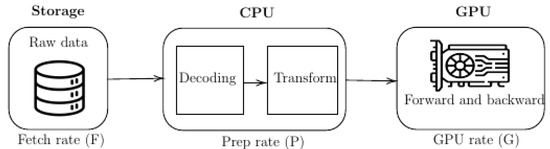
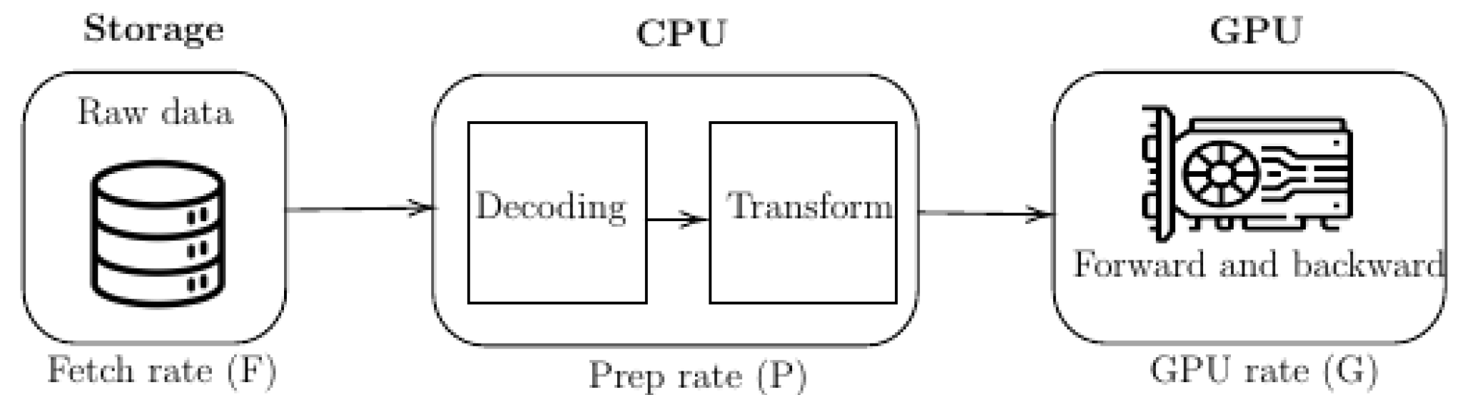
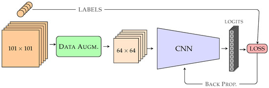
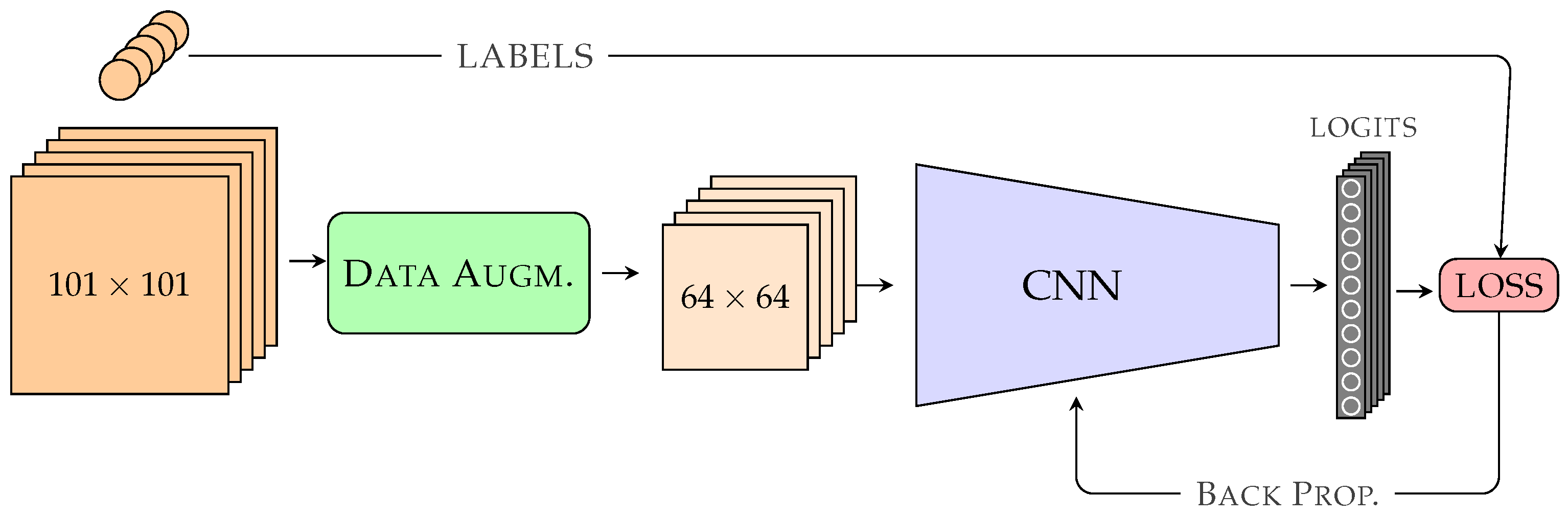
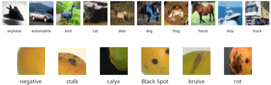
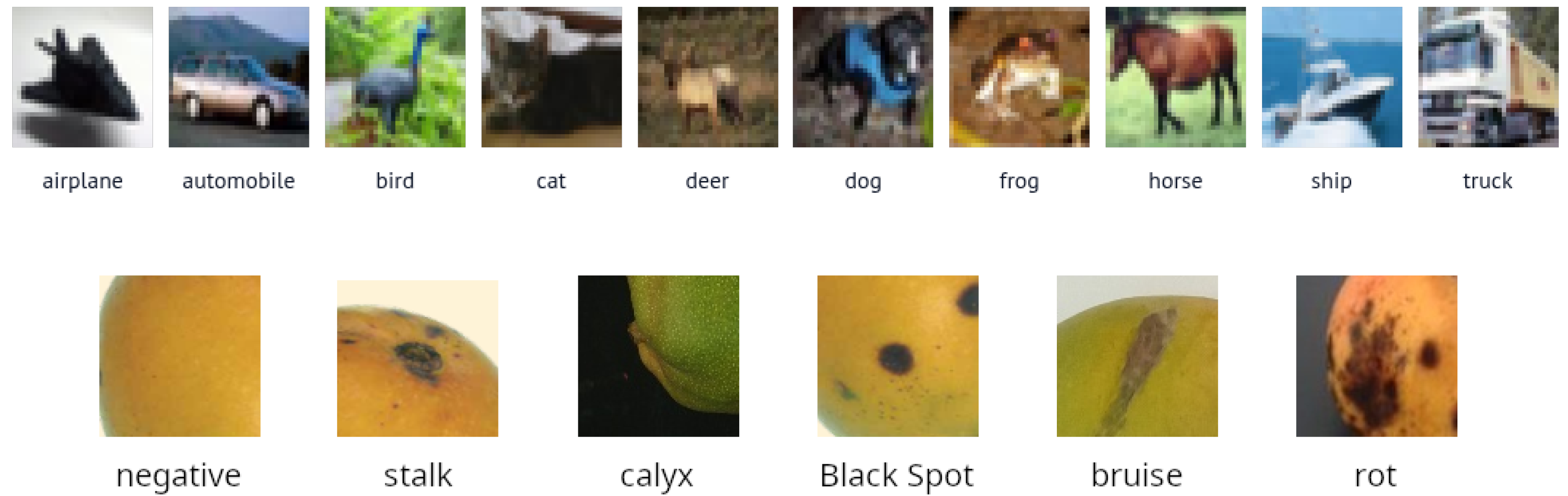
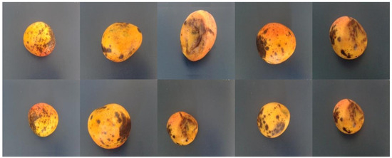
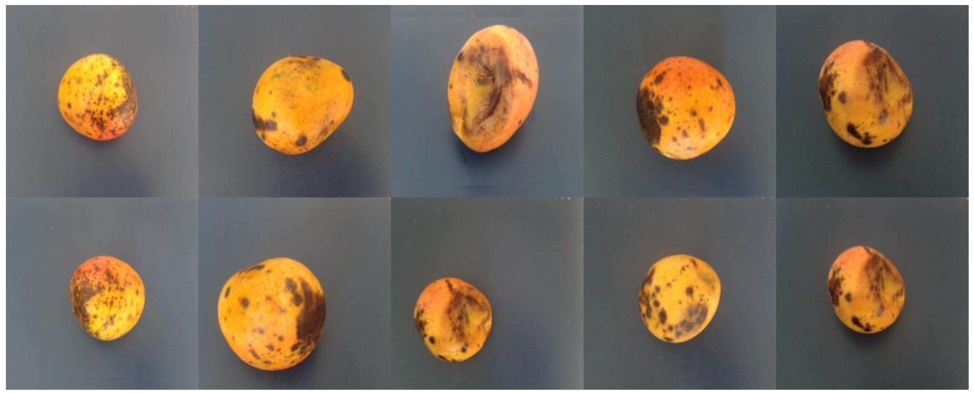
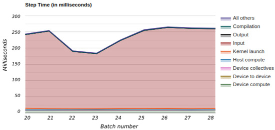
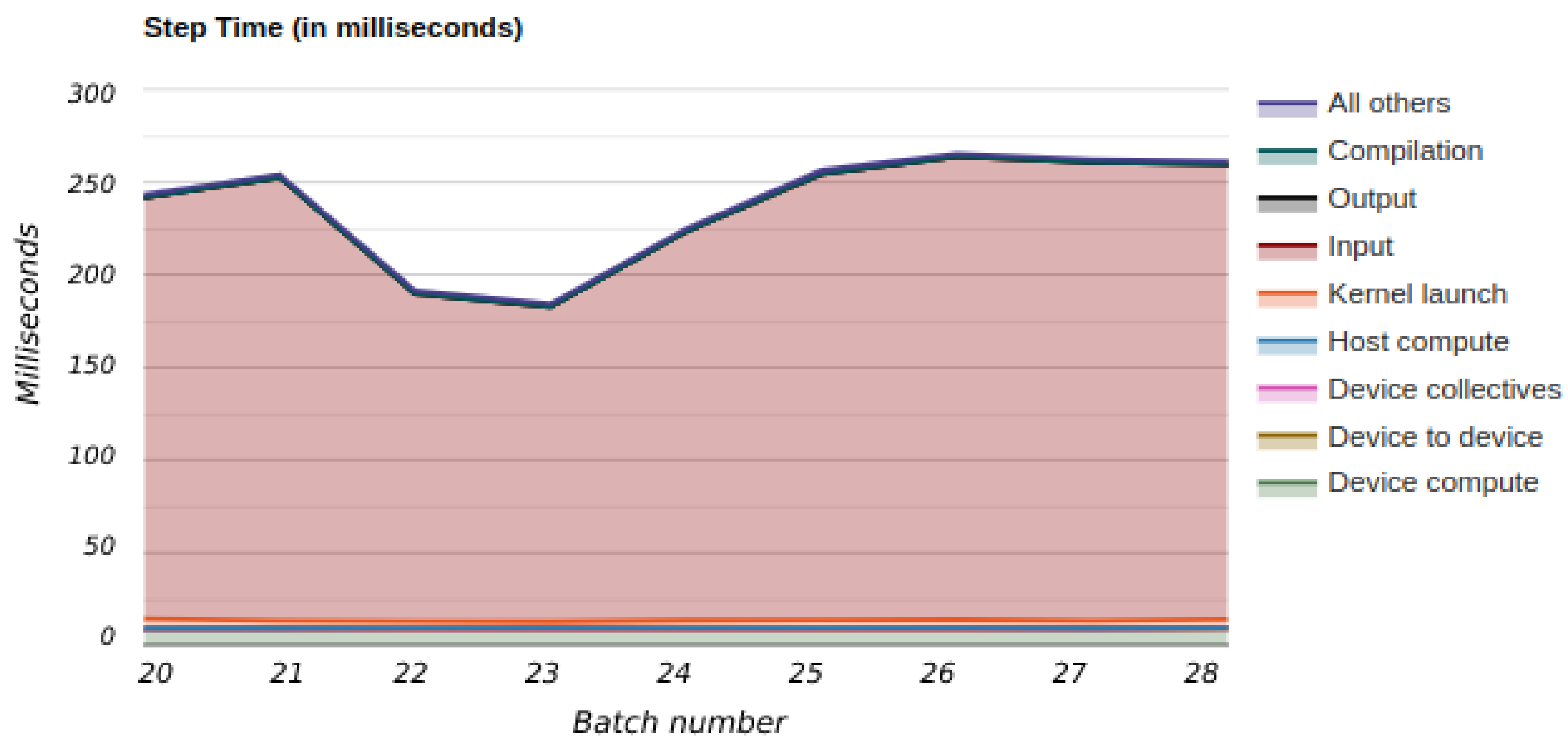
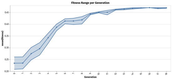
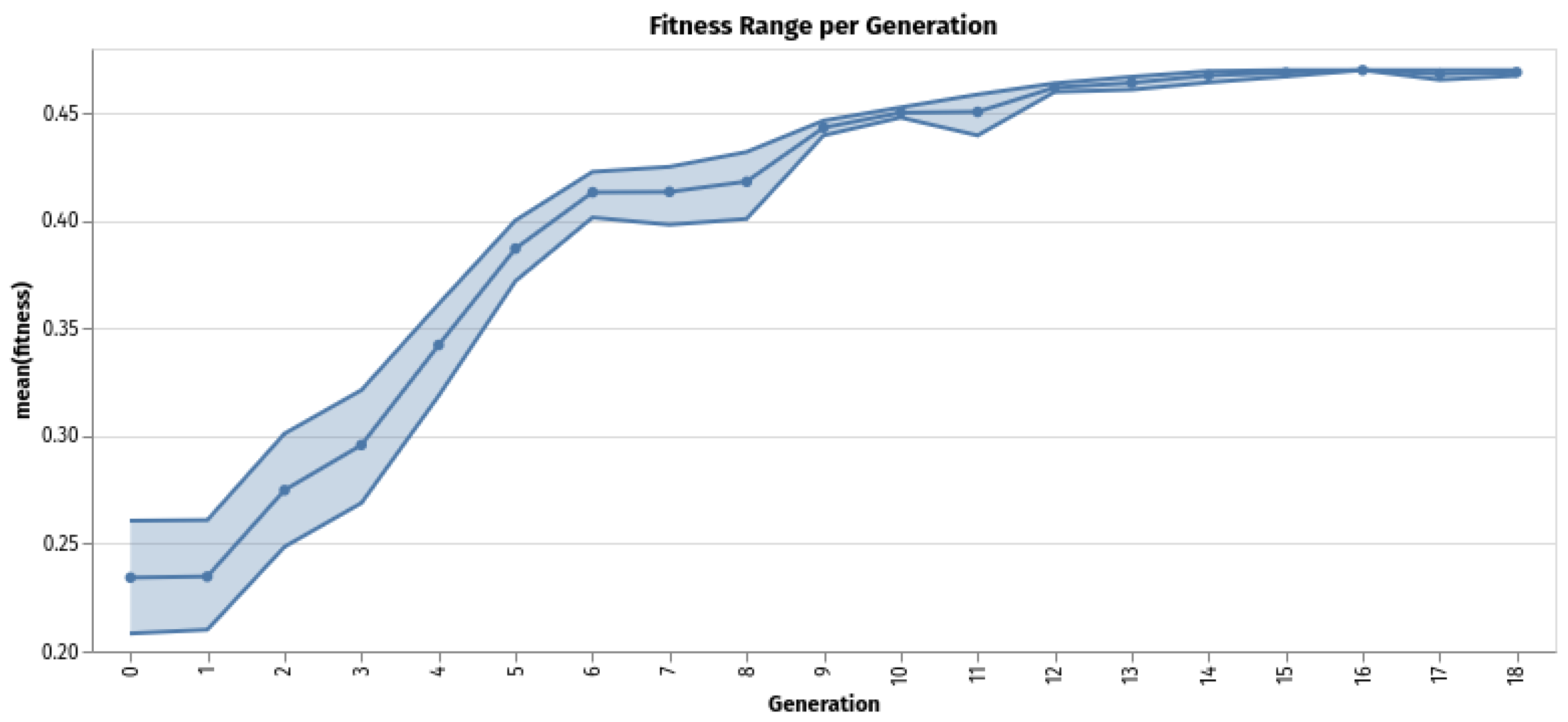
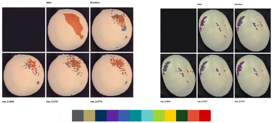
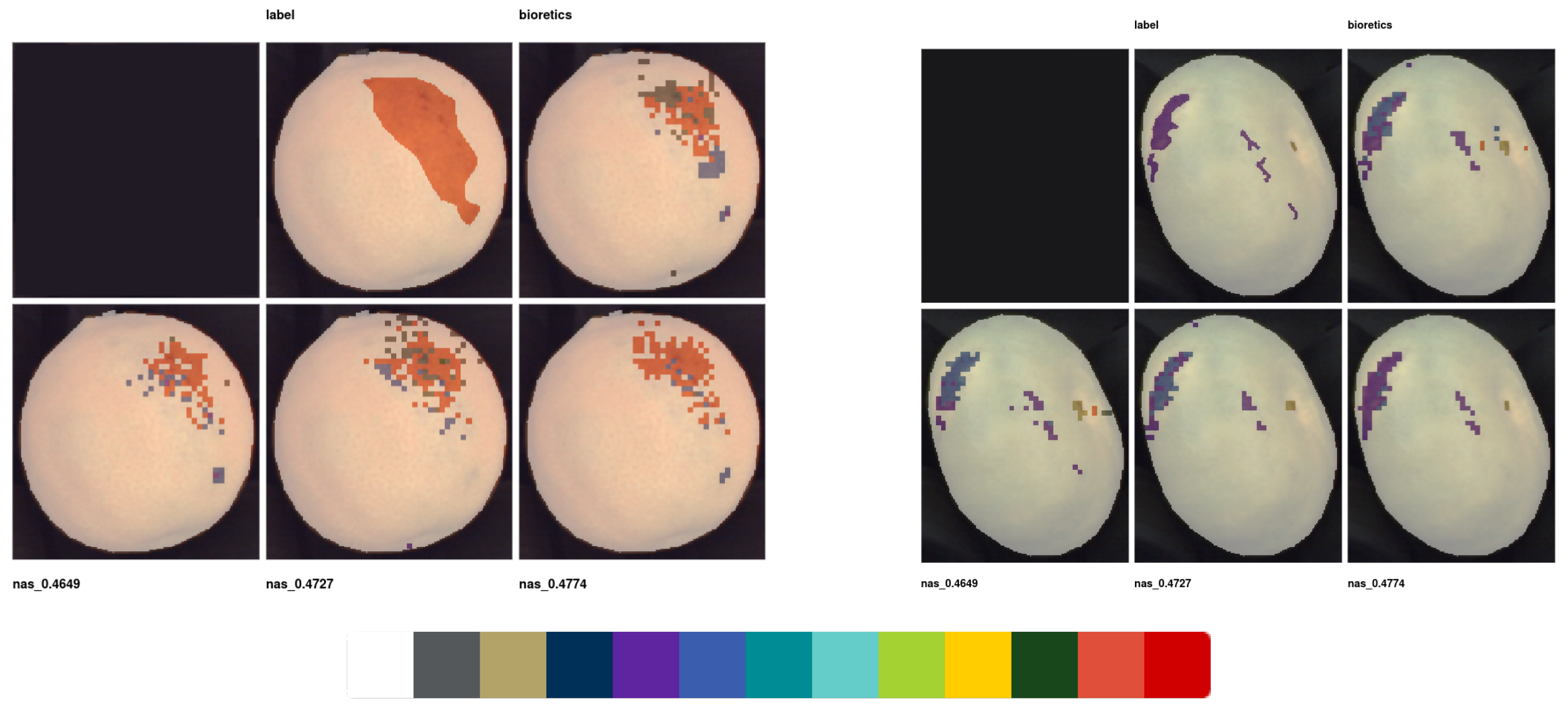

Disclaimer/Publisher’s Note: The statements, opinions and data contained in all publications are solely those of the individual author(s) and contributor(s) and not of MDPI and/or the editor(s). MDPI and/or the editor(s) disclaim responsibility for any injury to people or property resulting from any ideas, methods, instructions or products referred to in the content. |
© 2026 by the authors. Licensee MDPI, Basel, Switzerland. This article is an open access article distributed under the terms and conditions of the Creative Commons Attribution (CC BY) license.