Semantic Segmentation of Coffee Crops with PlanetScope Images: A Comparative Analysis of Spectral Band Combinations for U-Net Architecture

Abstract

Coffee is among the primary agricultural commodities in international trade; however, mapping coffee crops in mountainous regions faces limitations due to high spectral variability and complex canopy structures. This study hypothesized that optimized spectral band combinations focused on the visible spectrum may outperform configurations including near-infrared (NIR) for coffee crop segmentation. This work aimed to evaluate how different spectral band combinations affect the performance of the U-Net for segmenting coffee crops in mountainous regions. Seven PlanetScope images (4 m resolution) from Matas de Minas, Brazil, covering different phenological stages in 2023–2024, were divided into 316 training patches and 25 test patches of 256 × 256 pixels and used to train U-Net models across five spectral band combinations: (B, G, R), (B, G, NIR), (B, R, NIR), (G, R, NIR), and (B, G, R, NIR). The visible spectrum combination (B, G, R) demonstrated superior performance with an overall Accuracy of 0.8669 and, for the Coffee Crops class, an F1-score of 0.8682 and an IoU of 0.7671, outperforming all NIR-inclusive configurations. Visible bands’ sensitivity to pigmentation variations proved more effective in heterogeneous environments, while NIR increased spectral confusion near native vegetation and crop edges. The model overestimated cultivated area by 18.3% due to mixed pixels from 4 m resolution and mountainous terrain. These findings confirm that visible-spectrum bands offer a cost-effective alternative for coffee segmentation, though higher spatial resolution is needed for improved boundary delineation.

1. Introduction

Coffee is one of the most popular and daily consumed beverages worldwide, and constitutes one of the main agricultural commodities in international trade [1]. Coffee production supports approximately 25 million families, most of whom are small-scale producers who rely on coffee as their primary source of income [2]. Furthermore, coffee plays a fundamental economic role in several nations, being cultivated in approximately 80 countries located in tropical regions [3].

Given its socioeconomic relevance, estimating the area under coffee cultivation is essential for monitoring and planning at regional and national scales. This data helps in understanding production dynamics and monitoring the expansion of cultivated areas. It aids production chain planning and land use monitoring actions [4]. Estimation of cultivated areas is crucial for forecasting production and supporting public policies to stabilize the domestic market [5,6]. For government agencies, this information is strategic for monitoring and mitigating risks. It supports protective measures for coffee cultivation and national trade, especially during disasters or market fluctuations [7].

Traditionally, mapping of areas cultivated with coffee has been performed through visual interpretation of remote sensing images, with support from Geographic Information System (GIS) tools. With the advancement of remote sensing, images from different data sources have been employed. These include optical multispectral sensors, synthetic aperture radar (SAR) sensors, and unmanned aerial vehicle (UAV) platforms equipped with multispectral cameras [6,8,9]. From these images, the most common methods for automatic image classification are the maximum likelihood classifier [10,11], machine learning algorithms [12,13], and texture analysis-based methods such as gray-level co-occurrence matrix (GLCM) [14,15]. Deep learning-based methods are also used [16,17]. Although they yield consistent results in specific contexts, these methods face limitations in large-area mapping. This is primarily due to the high spectral and structural variability of coffee crops, as well as the difficulty in accurately representing their semantic complexity.

The determination of area cultivated with coffee becomes even more complex due to variations in size, shape, and spectral characteristics of coffee plantations, which make distinguishing them from other land-cover classes difficult. This problem is even more complex when mapping involves mountainous regions due to greater diversity of ground cover, small and fragmented cultivation areas, presence of native vegetation, and neighboring crops with spectral responses similar to coffee in addition to topographic influence that modifies target reflectance and amplifies confusion between classes [18,19]. This complexity leads traditional segmentation algorithms, such as those based on thresholding, edges, regions, and graphs, to present limited performance [20]. In addition to having a high computational cost, these methods cannot always strike a balance between efficiency and precision, proving inadequate for dealing with the visual specificity of coffee plantations.

In this context, deep learning techniques have emerged as an efficient alternative for the automatic identification of agricultural areas [14,21,22,23,24]. Among the most promising approaches for this application, semantic segmentation stands out, which involves classifying each pixel of an image by assigning it a specific class, while considering the spatial context and relationships between neighboring pixels, thereby allowing for the precise identification of different land cover classes. Recent studies have shown that, in data with high spatial resolution and low spectral quality, deep neural networks can capture complex high-level semantic features [25,26,27,28,29]. This succeeds in overcoming recurring limitations in land cover classification, particularly those involving visually similar elements with distinct spectral signatures or distinct elements with similar signatures [21]. Thus, deep neural networks extract more discriminative information, significantly improving the accuracy of identifying specific crops, such as coffee.

Among the deep neural network architectures applied to semantic segmentation in remote sensing, U-Net has stood out due to its encoder–decoder architecture combined with skip connections, which preserve spatial information from different levels of abstraction and allow the extraction of low and high-level features [30]. These characteristics facilitate the identification of complex patterns in agricultural areas comprising irregular parcels with high spectral heterogeneity. In mapping crop areas, U-Net has demonstrated its potential to capture both canopy structures and spatial distribution patterns, which are essential aspects for crop delineation [31,32].

In addition to the ability of deep neural networks to extract complex semantic and spatial features, adequate selection of input bands is essential for land cover segmentation performance [33]. Each type of cover exhibits its own reflectance behavior across the electromagnetic spectrum, enabling differentiation through specific band combinations [34,35,36]. In this context, PlanetScope satellite images, which have spatial resolution between 3 and 4.1 m, depending on altitude, possess four spectral bands—blue, green, red, and near-infrared—which provide data capable of representing the spectral variability of vegetation and different types of land cover [37]. Although many deep learning models are originally designed to process three spectral channels, it is possible to adapt them to receive a larger number of bands, making the selection and combination of these bands determining factors for segmentation performance.

Despite these advances, a research gap remains. The systematic evaluation of how specific spectral band combinations affect deep learning performance for coffee crop seg-mentation in mountainous regions with high spectral heterogeneity has not been adequately addressed. Most studies use all available bands. They do not investigate whether band selection could optimize segmentation outcomes for perennial crops with complex canopy structures.

The central hypothesis of this work is that, for a perennial crop with a complex canopy structure such as coffee, not all bands contribute equally to the segmentation task. An optimized combination of bands, possibly focused on the visible spectrum, may outperform configurations that include near-infrared. Given this scenario, this work aimed to evaluate how different spectral band combinations affect the performance of the U-Net for coffee crop segmentation in mountainous regions.

The main contributions of this study are:

(i) A systematic comparison of five spectral band combinations for U-Net-based coffee crop segmentation, demonstrating that visible spectrum bands (B, G, R) outperform all configurations including NIR in mountainous regions;

(ii) A quantitative spectral separability analysis using Jeffries-Matusita distance that provides a physical and mechanistic interpretation of band performance differences;

(iii) Practical evidence that cost-effective visible-spectrum sensors are sufficient for accurate coffee mapping, reducing dependency on multispectral instruments.

2. Materials and Methods

2.1. Study Area and Images Used

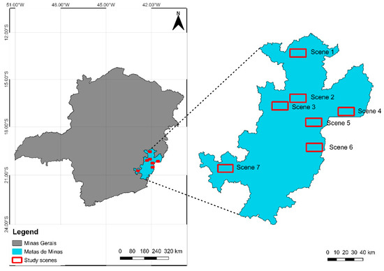
The study was conducted in the region known as Matas de Minas, Minas Gerais, Brazil, as indicated in Figure 1. This region received the Geographical Indication concession of the “Indication of Origin” type, in 2020. Geographical Indication is a registration granted in Brazil by the National Institute of Industrial Property (INPI), which officially recognizes the reputation or quality of a product or service linked to its geographical origin. It can be classified as either an Indication of Origin or a Denomination of Origin [38]. This region spans an area of 17,633.18 km², comprising 64 municipalities, and is characterized by mountainous and highly undulating terrain. Much of the territory has altitudes ranging between 400 and 1000 m; however, there are locations that exceed 2000 m [38].

Figure 1. Location of the study area. The region in blue corresponds to Matas de Minas, while the areas in red highlight the seven selected scenes (Scenes 1 to 7).

PlanetScope remote sensing images (produced by Planet Labs Inc., San Francisco, CA, USA) were obtained through the Planet Explorer version 2.3.3 plugin, available in QGIS software, version 3.22.1 [39]. Areas of interest were delineated using a reference vector layer, and corresponding images were then downloaded directly into QGIS. Seven scenes were selected, each represented by a single image. Thus, seven images were used in the analysis. Each scene is a distinct geographical location, ensuring spatial diversity in the training data. Selecting one image per scene prevents temporal autocorrelation and maximizes spatial coverage. Using several temporally correlated images from the same location can inflate model performance estimates due to spatial autocorrelation between training and test samples [40,41,42]. Preliminary experiments confirmed that including multiple images from the same scene did not improve test performance, since these images provided redundant rather than new discriminative information. Thus, selecting a single image per scene ensured independent observations across locations while capturing phenological variability of coffee crops throughout the production cycle.

Images were acquired in different months of 2023 and 2024, specifically in December, February, April, June, July, August, and October. This approach covers different phenological stages of the crop, reflecting variations in physiological conditions and plants reflectance throughout the production cycle. Images have a pixel size of 4 m and are composed of four spectral bands: blue (455–515 nm), green (500–590 nm), red (590–670 nm), and near-infrared (780–860 nm) [37]. All images were acquired as Surface Reflectance products, which are atmospherically corrected by Planet Labs prior to distribution, ensuring radiometric consistency across multi-temporal acquisitions. Figure 1 illustrates the spatial distribution of these scenes.

2.2. Model Development

For model construction, scenes used for training and testing were randomly selected to ensure impartiality in data selection and avoid spatial bias. As a result, scenes 1, 2, 4, 5, 6, and 7 were assigned to the training process, while scene 3 was reserved for testing the final model after training. By reserving a complete, spatially independent scene for testing, the study provides a realistic estimate of the model’s generalization, ensuring independence between the training and test data. The adopted workflow comprised the following steps: (i) labeling images from all scenes, (ii) data preprocessing, including mask generation, patch partitioning, and normalization, and (iii) training the U-Net architecture with different combinations of the four spectral bands. Model implementation was performed in Python language (version 3.13), employing TensorFlow and Keras libraries for building and training the deep learning architecture, Rasterio and GeoPandas for processing geospatial data, NumPy for matrix operations, and Scikit-learn for calculating evaluation metrics.

2.2.1. Labeling

Labeling consisted of creating vector polygons that encompass each class. Two classes were defined: Coffee Crops, corresponding to areas cultivated with coffee, and Background, encompassing all other surfaces without visual characteristics compatible with the class of interest. Labeling was performed using visual interpretation from images of the seven selected scenes (1–7).

The labeling process was conducted in QGIS software, version 3.22.1 [39], using shapefile format, with the WGS 84 coordinate system, the same adopted in the images. The steps comprised: (i) loading PlanetScope images in QGIS; (ii) creating a polygon-type vector layer for the Coffee Crops class; (iii) visual identification of the Coffee Crops class through interpretation of visual characteristics in images; (iv) manual delimitation of class contours through polygon digitization, using vector drawing tools available in the software; and (v) review and adjustment of created polygons to ensure consistency and accuracy of annotations.

2.2.2. Data Preprocessing

Vector polygons from the labeling stage were used to create binary masks for the defined classes: Coffee Crops (class 1) and Background (class 0). This process converted the polygons into matrices for compatibility with neural network input. It also ensured spatial alignment between the multispectral TIFF images and their masks.

After generating the binary masks, multispectral images and these masks were loaded and organized into batches to optimize memory usage. Subsequently, five spectral band combinations were evaluated as model input: four three-band combinations (B, G, R), (B, G, NIR), (B, R, NIR), (G, R, NIR), and one four-band combination (B, G, R, NIR). The acronyms B, G, R, and NIR refer to blue, green, red, and near-infrared spectral bands.

Images and masks were partitioned into 256 × 256 pixel patches with a stride of 256 pixels. These are small sub-images extracted from the main image without overlap. Preliminary tests considered using overlapping patches, but this did not improve validation performance and increased training time. Therefore, the method without overlap was chosen to optimize computational efficiency.

During partitioning, only patches with at least one pixel of the Coffee Crops class were kept. Patches composed exclusively of the Background class were discarded. This decision avoids generating samples only of the Background class, which do not contribute to model learning. It also helps prevent excessive data imbalance and improves the network’s ability to learn relevant patterns for detecting Coffee Crops. Including all pure background patches would result in a highly unbalanced dataset, potentially biasing the model towards the majority class and reducing its ability to detect the class of interest, Coffee Crops.

This partitioning produced 316 patches of 256 × 256 pixels for the training set and 25 patches for the test set. Next, pixel values were normalized to the [0, 1] interval by dividing each pixel by the global maximum reflectance value for its spectral band, calculated from the entire dataset. To ensure radiometric consistency, this global maximum-based normalization provided a uniform value scale for all neural network input samples. Table 1 summarizes the dataset composition for the training and test sets. Finally, a data generator provided patches in batches during training and testing. This optimized memory use and guaranteed a continuous sample flow throughout modeling.

Table 1. Summary of dataset composition for training and test sets.

Set	Scenes	Patches	Coffee Crops Pixels	Background Pixels	Total Pixels
Training	1,2,4,5,6,7	316	4,580,165	16,129,211	20,709,376
Test	3	25	447,296	1,191,104	1,638,400
Total	1–7	341	5,027,461	17,320,315	22,347,776

Although the test set comprises a single scene, it contains 1,638,400 classified pixels, providing a relatively large sample for evaluating pixel-level performance in semantic segmentation. Furthermore, using a complete, spatially independent scene preserves landscape heterogeneity and prevents data breach between the training and test sets.

2.2.3. Modeling

In this study, the U-Net semantic segmentation network [30] was used to build the coffee crop identification model. U-Net was selected for this comparative study due to its proven effectiveness in agricultural remote sensing applications, its encoder–decoder architecture with skip connections that preserve spatial information crucial for boundary delineation, and its ability to achieve good performance with relatively small training datasets [30]. The focus of this work is on evaluating spectral band combinations rather than architectural innovations, making the U-Net an appropriate baseline architecture. For each tested spectral band combination, a model was trained from scratch for 50 epochs, a value determined by preliminary experiments that showed convergence before this epoch with the Adam optimizer and the binary cross-entropy loss function. The batch size was set to 8 for memory optimization, and no data augmentation techniques were applied.

Model training was performed using CPU resources available on the Federal University of Viçosa (UFV) cluster. The cluster’s head node has an Intel Xeon Gold 6212U processor with 24 cores and 48 threads, operating at 2.40 GHz. It also includes 512 GB of DDR4 RAM at 3200 MT/s. This environment coordinated computational tasks and provided resources for data processing and model execution.

During training, Keras callbacks were implemented for process control and optimization. ModelCheckpoint automatically saved the model at each epoch if performance improved, based on the Loss. ReduceLROnPlateau reduced the learning rate by 0.1 if the Loss stagnated for five epochs. The initial learning rate was 1 × 10⁻⁴, and the minimum was 1 × 10⁻¹⁰. The best model for each band combination was saved and used for evaluation on the test set. Although the training set had only 316 patches, the effective sample size is about 20.7 million classified pixels (Table 1). These callbacks serve as implicit regularization, helping reduce the risk of overfitting.

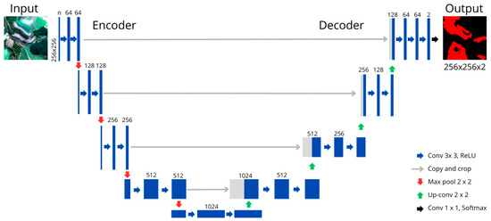
The U-Net architecture used here followed the original structure [30]. It had an encoder path and a decoder path. The encoder extracted features with four blocks, each containing two convolution layers followed by max pooling. The decoder recovered image resolution using upsampling and two convolution layers. Skip connections linked the encoder and decoder blocks to preserve spatial information throughout the network.

The U-Net implemented here was adjusted to receive 256 × 256 pixel patches with 3 or 4 spectral bands. The output was set for two classes: Coffee Crops and Background. This adaptation maintained the network’s suitability for the task, preserving the U-Net’s structural organization, depth, and information flow.

Figure 2 presents the adapted U-Net architecture used in this work, based on the version proposed by [43]. The structure consisted of an encoder path and a decoder path, interconnected by skip connections that preserved spatial information. The input consisted of 256 × 256 pixel patches, with “n = 3 or 4” spectral bands. The output was a binary segmentation mask, where the Coffee Crops and Background classes are represented in red and black, respectively, in Figure 2.

Figure 2. U-Net architecture adapted for coffee crop segmentation from PlanetScope sensor multispectral images. In the segmentation output, red represents Coffee Crops areas and black represents Background.

2.2.4. Evaluation Metrics

Model evaluation was conducted from analysis of results obtained by the U-Net architecture on the test set, considering different spectral band combinations: (B, G, R), (B, G, NIR), (B, R, NIR), (G, R, NIR), and (B, G, R, NIR). To quantify segmentation performance, the following metrics were used: Accuracy, which represents the total proportion of correctly classified pixels in relation to total evaluated pixels; F1-score, which provides a balanced measure that combines Precision and Recall, reflecting the relationship between false positives and false negatives; and Intersection over Union (IoU). Accuracy was used as a general measure of model performance. F1-score was chosen for being a harmonic mean between Precision and Recall, offering robust evaluation even in scenarios with class imbalance. Finally, Intersection over Union (IoU), a standard metric in semantic segmentation tasks, was employed to evaluate the spatial overlap between the prediction and ground truth masks, more rigorously penalizing contour and localization errors. The calculation form for Accuracy, F1-score, Precision, Recall, and IoU are presented in Equations (1)–(5).

$$\mathrm{A}\mathrm{c}\mathrm{c}\mathrm{u}\mathrm{r}\mathrm{a}\mathrm{c}\mathrm{y}={\displaystyle \frac{\mathrm{T}\mathrm{P}+\mathrm{T}\mathrm{N}}{\mathrm{T}\mathrm{P}+\mathrm{T}\mathrm{N}+\mathrm{F}\mathrm{P}+\mathrm{F}\mathrm{N}}}$$

(1)

$$\mathrm{F}1-\mathrm{s}\mathrm{c}\mathrm{o}\mathrm{r}\mathrm{e}=2\times {\displaystyle \frac{\mathrm{P}\mathrm{r}\mathrm{e}\mathrm{c}\mathrm{i}\mathrm{s}\mathrm{i}\mathrm{o}\mathrm{n}\times \mathrm{R}\mathrm{e}\mathrm{c}\mathrm{a}\mathrm{l}\mathrm{l}}{\mathrm{P}\mathrm{r}\mathrm{e}\mathrm{c}\mathrm{i}\mathrm{s}\mathrm{i}\mathrm{o}\mathrm{n}+\mathrm{R}\mathrm{e}\mathrm{c}\mathrm{a}\mathrm{l}\mathrm{l}}}$$

(2)

$$\mathrm{P}\mathrm{r}\mathrm{e}\mathrm{c}\mathrm{i}\mathrm{s}\mathrm{i}\mathrm{o}\mathrm{n}={\displaystyle \frac{\mathrm{T}\mathrm{P}}{\mathrm{T}\mathrm{P}+\mathrm{F}\mathrm{P}}}$$

(3)

$$\mathrm{R}\mathrm{e}\mathrm{c}\mathrm{a}\mathrm{l}\mathrm{l}={\displaystyle \frac{\mathrm{T}\mathrm{P}}{\mathrm{T}\mathrm{P}+\mathrm{F}\mathrm{N}}}$$

(4)

$$\mathrm{I}\mathrm{o}\mathrm{U}={\displaystyle \frac{\mathrm{T}\mathrm{P}}{\mathrm{T}\mathrm{P}+\mathrm{F}\mathrm{P}+\mathrm{F}\mathrm{N}}}$$

(5)

where TP (True Positive) represents the number of pixels correctly classified as belonging to the positive class; TN (True Negative), pixels correctly classified as not belonging to the positive class; FP (False Positive), pixels incorrectly classified as belonging to the positive class; and FN (False Negative), pixels incorrectly classified as not belonging to the positive class.

Additionally, confusion matrices were generated for each spectral band combination, allowing for the evaluation of the distribution of model hits and misses between the Coffee Crops and Background classes. This analysis complemented quantitative metrics by evidencing incorrect classification patterns, such as overestimation of coffee areas or confusion with other land covers, in addition to allowing comparative visualization of the performance obtained in each evaluated spectral combination. With this set of procedures, a methodological basis was established for analyzing the results, allowing for a detailed understanding of the impact of spectral band selection on U-Net performance in coffee crop segmentation.

2.2.5. Spectral Separability Analysis

Beyond evaluating model performance, a spectral separability analysis quantified how well each PlanetScope band distinguishes Coffee Crops from Background at the pixel level. This independent assessment of spectral band contributions complements U-Net segmentation metrics.

Spectral statistics, such as mean and standard deviation, were calculated for Coffee Crops and Background across all four bands. First, to ensure a consistent analysis pipeline, pixel values were extracted from 316 training and 25 test patches, totaling 22,347,776 classified pixels. Next, all values were normalized to [0, 1] using the same global maximum-based approach from preprocessing (Section 2.2.2), thereby aligning the separability metrics with model inputs. Finally, for each band, the Jeffries–Matusita (JM) distance was calculated as a measure of class separability, as described by [43], following Equation (6):

$${\mathrm{J}\mathrm{M}}_{\mathrm{i}\mathrm{j}}=2\left(1-{\mathrm{e}}^{-\mathrm{B}}\right)$$

(6)

where B is the Bhattacharyya distance, defined as:

$$\mathrm{B}={\displaystyle \frac{1}{8}}{\left({\mathrm{m}}_{\mathrm{i}}-{\mathrm{m}}_{\mathrm{j}}\right)}^{\mathrm{t}}{\left\{{\displaystyle \frac{{\mathsf{\Sigma }}_{\mathrm{i}}+{\mathsf{\Sigma }}_{\mathrm{j}}}{2}}\right\}}^{-1}\left({\mathrm{m}}_{\mathrm{i}}-{\mathrm{m}}_{\mathrm{j}}\right)+{\displaystyle \frac{1}{2}}\mathrm{l}\mathrm{n}\left\{{\displaystyle \frac{\left|\frac{{\mathsf{\Sigma }}_{\mathrm{i}}+{\mathsf{\Sigma }}_{\mathrm{j}}}{2}\right|}{\left({\left|{\mathsf{\Sigma }}_{\mathrm{i}}\right|}^{\frac{1}{2}}{\left|{\mathsf{\Sigma }}_{\mathrm{j}}\right|}^{\frac{1}{2}}\right)}}\right\}$$

(7)

In Equation (7), m_i and m_j represent the mean spectral values for the Coffee Crops and Background classes, respectively, while Σ_i and Σ_j denote their corresponding covariance matrices and the superscript t indicates the transpose operation.

3. Results

3.1. Developed Model

We evaluated U-Net performance on the test set for five spectral band combinations. Table 2 shows the global evaluation metrics (Accuracy, Precision, Recall, F1-score, and IoU) used to compare the tested combinations.

Table 2. General U-Net performance metrics considering both classes of the test set, for different evaluated spectral band combinations.

Band Combination	Accuracy	Precision	Recall	F1-Score	IoU
(B, G, R)	0.8669	0.8670	0.8669	0.8668	0.7650
(B, G, NIR)	0.8039	0.8084	0.8039	0.8032	0.6714
(B, R, NIR)	0.8376	0.8377	0.8376	0.8375	0.7205
(G, R, NIR)	0.8309	0.8310	0.8309	0.8309	0.7108
(B, G, R, NIR)	0.8494	0.8495	0.8494	0.8493	0.7381

Bold numbers indicate that the spectral band combination has the best overall performance.

Results demonstrate that band combinations (B, G, R) and (B, G, R, NIR) presented superior performance, with the highest values in all evaluated metrics. The (B, G, R) combination stood out as the best overall configuration, with an accuracy of 0.8669 and IoU of 0.7650, followed by the combination (B, G, R, NIR), which obtained an accuracy of 0.8494 and IoU of 0.7381. In contrast, combination (B, G, NIR) presented the lowest performance among all evaluated configurations, with an accuracy of 0.8039 and an IoU of 0.6714.

For a more detailed comparison of performance in the Coffee Crops class segmentation, Table 3 presents the specific metrics for this class by spectral band combination. The results reaffirm the superiority of (B, G, R), which outperformed all others with a Recall of 0.8769, Precision of 0.8596, F1-score of 0.8682, and IoU of 0.7671. The (B, G, R, NIR) combination followed closely, with Precision (0.8572) and F1-score (0.8477) nearly matching the highest values. In contrast, (B, R, NIR), (G, R, NIR), and (B, G, NIR) performed worse, especially the last two, which had the lowest F1-score and IoU values.

Table 3. U-Net performance metrics specifically for the Coffee Crops class, obtained from the test set, in different spectral band combinations.

Band Combination	Recall	Precision	F1-Score	IoU
(B, G, R)	0.8769	0.8596	0.8682	0.7671
(B, G, NIR)	0.8637	0.7715	0.8150	0.6878
(B, R, NIR)	0.8475	0.8310	0.8392	0.7229
(G, R, NIR)	0.8239	0.8357	0.8297	0.7090
(B, G, R, NIR)	0.8384	0.8572	0.8477	0.7356

Bold values indicate, in each column, the spectral band combination that obtained the best performance for the Coffee Crops class in the respective metric.

It is worth noting that incorporating the NIR band into the complete set (B, G, R) did not result in improvements. On the contrary, a slight performance decline was observed for the Coffee Crops class in all evaluated metrics, with reductions in Recall from 0.8769 to 0.8384, Precision from 0.8596 to 0.8572, F1-score from 0.8682 to 0.8477, and IoU from 0.7671 to 0.7356. These results suggest that, for the data used, the NIR band did not contribute to the spectral differentiation of coffee crops.

3.2. Spectral Separability Results

To provide independent quantitative support for the model performance results, spectral separability between Coffee Crops and Background classes was evaluated using Jeffries-Matusita (JM) distance. In the visible spectrum, Coffee Crops exhibited consistently lower mean reflectance compared to Background (Blue: 0.034 against 0.040; Green: 0.065 against 0.074; Red: 0.044 against 0.055), while in NIR, Coffee Crops showed higher mean values (0.365 against 0.319), consistent with a healthy vegetation response. Both classes exhibited substantial NIR variability, with standard deviation (SD) values of 0.0825 and 0.0831 for Coffee Crops and Background, respectively, indicating high within-class heterogeneity.

Despite NIR showing the largest absolute difference between class means (Δ = |μ_Coffee − μ_Background| = 0.046), it had the lowest JM distance (0.274) due to high within-class variance, leading to substantial distribution overlap. Conversely, the individual Blue, Green, and Red bands achieved JM distances of 0.444, 0.422, and 0.391, respectively, representing values 43% to 62% higher than NIR. This indicates that visible bands provide superior pixel-level discrimination of coffee crops from the background in this study area.

Table 4 presents the separability metrics for the evaluated band combinations. The minimum JM distance within each combination identifies the least discriminative component, thereby constraining the overall spectral discrimination capacity. (B, G, R) presented a minimum JM of 0.391 (limited by the Red band), while all NIR-inclusive combinations presented a minimum JM of 0.274 (limited by the NIR band). This 43% difference in minimum separability indicates that NIR acts as a limiting factor for spectral discrimination when included in band combinations.

Table 4. Spectral separability metrics for evaluated band combinations based on Jeffries-Matusita (JM) distance.

Band Combination	Mean JM	Min JM	Max JM	Limiting Band
(B, G, R)	0.419	0.391	0.444	Red
(B, G, NIR)	0.380	0.274	0.444	NIR
(B, R, NIR)	0.370	0.274	0.444	NIR
(G, R, NIR)	0.362	0.274	0.422	NIR
(B, G, R, NIR)	0.383	0.274	0.444	NIR

Min JM represents the weakest discriminative band within each combination. Higher JM values indicate better separability.

3.3. Analysis of Prediction Patterns Between Classes

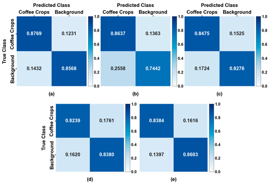
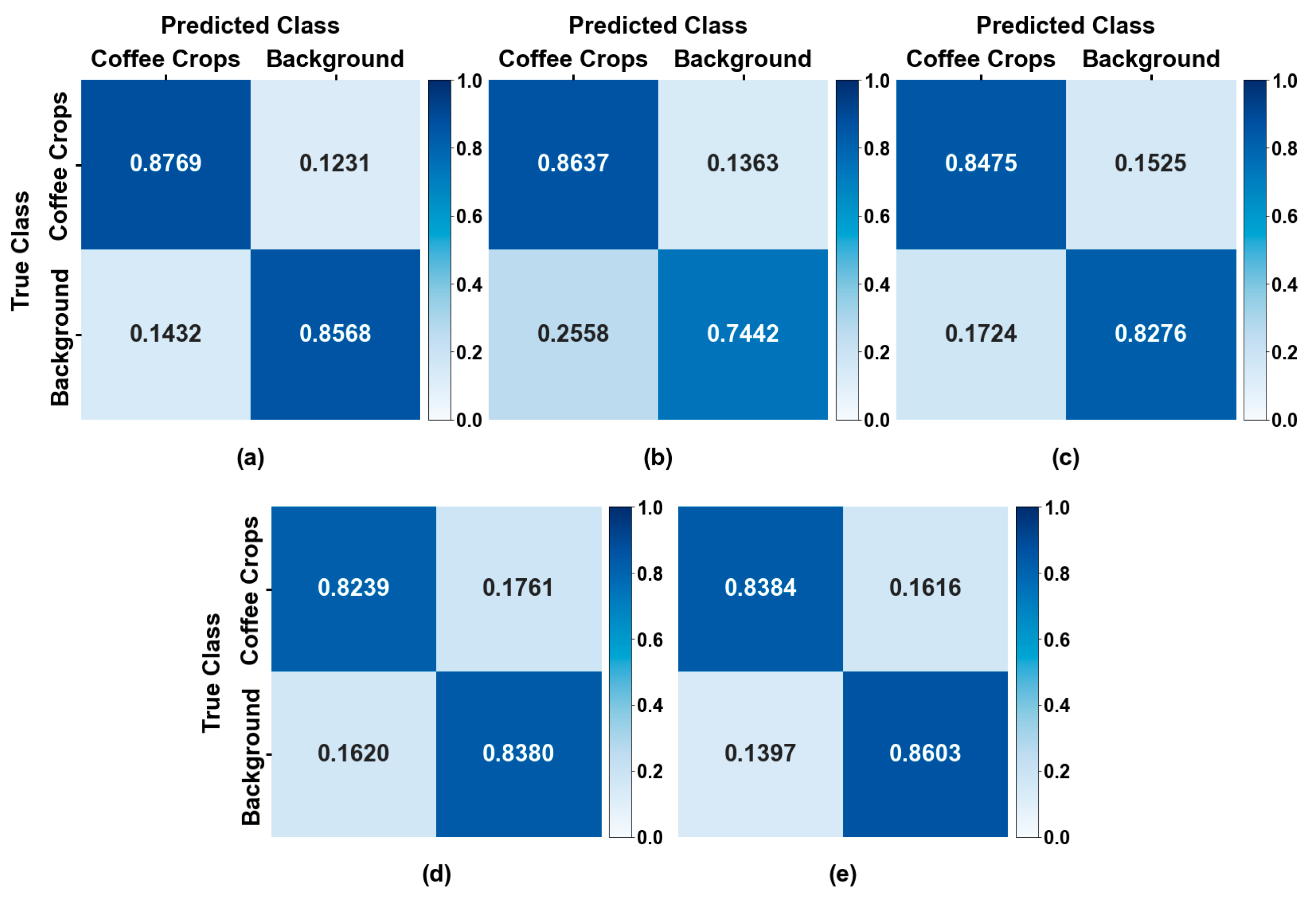
To better understand model performance in binary segmentation between Coffee Crops and Background classes, confusion matrices were generated for each spectral band combination. This analysis enabled the identification of the proportion of correctly classified pixels, as well as the most frequent errors between the two categories, contributing to a more precise diagnosis of the limitations of each spectral configuration. Confusion matrices, constructed from the test set, are presented in Figure 3.

Figure 3. Confusion matrices generated for each spectral band combination used as input in the U-Net architecture, evaluated on the test set: (a) combination (B, G, R); (b) combination (B, G, NIR); (c) combination (B, R, NIR); (d) combination (G, R, NIR); (e) combination (B, G, R, NIR).

Among all combinations evaluated, (B, G, R) demonstrated the best balance in predicting accuracy between classes: the hit rate for Coffee Crops was 0.8769 and for Background 0.8568, with confusion rates of 0.1231 and 0.1432, respectively. By comparison, when R was replaced by NIR in the (B, G, NIR) combination, the hit rate for Background dropped to 0.7442 and the confusion rate increased to 0.2558, illustrating a reduction in the model’s ability to distinguish non-coffee areas. This clarifies the direct impact of swapping bands in the combinations.

The (B, R, NIR) and (G, R, NIR) combinations performed at an intermediate level, with similar hit rates for both classes: 0.8475 and 0.8239 for Coffee Crops, and 0.8276 and 0.8380 for Background, respectively. Finally, the four-band combination (B, G, R, NIR) achieved a Coffee Crops hit rate of 0.8384 and a Background hit rate of 0.8603, with confusion rates of 0.1616 and 0.1397. This confirms that adding the NIR band to the configuration (B, G, R) did not provide performance gains in segmentation between classes.

3.4. Comparative Analysis of Segmentation Masks

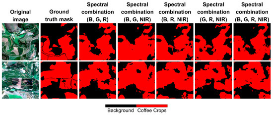
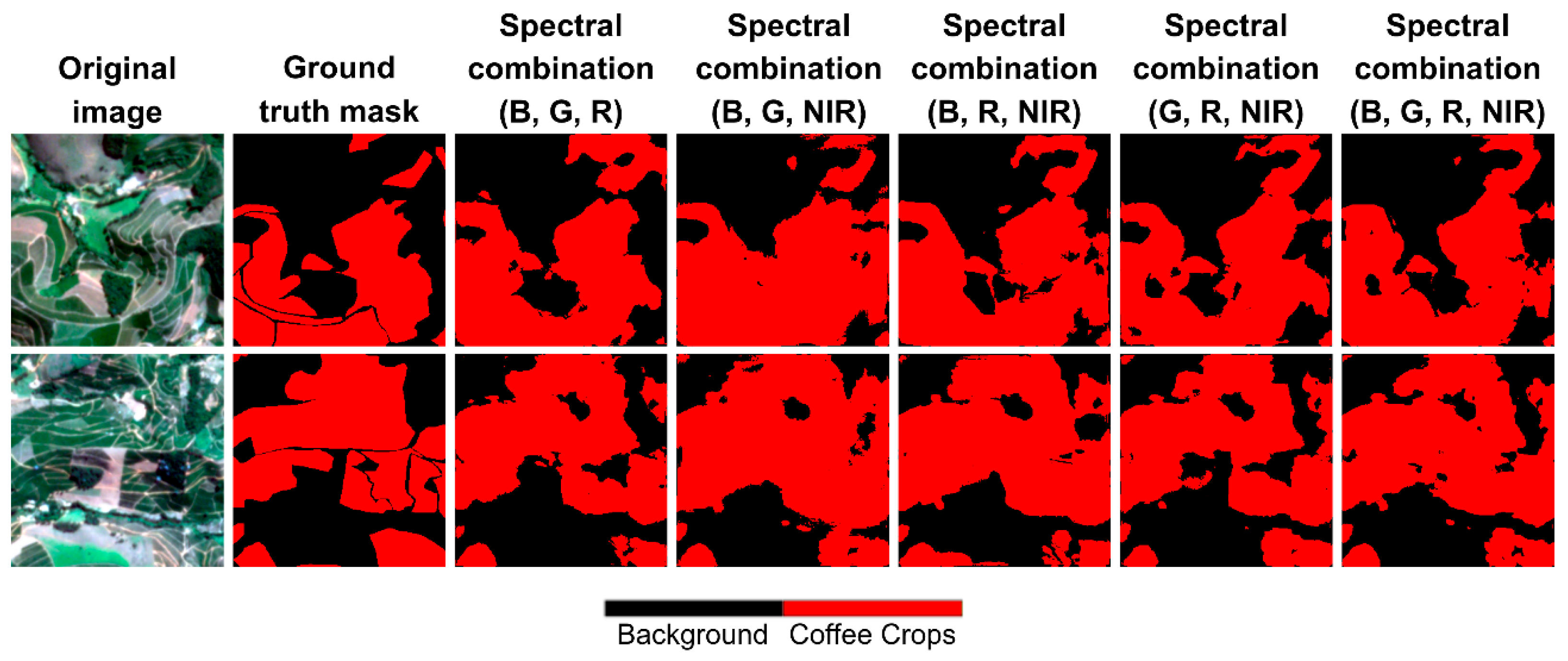
Finally, in addition to quantitative evaluation, a qualitative analysis of segmentation masks produced by the U-Net architecture was performed. Figure 4 presents, for the same patch from the test area, the original image, ground truth mask, and predicted masks for each of the five spectral combinations: (B, G, R), (B, G, NIR), (B, R, NIR), (G, R, NIR), and (B, G, R, NIR). This approach enables a comparative visual evaluation of models on the test set, allowing for verification of the quality of coffee crop segmentation.

Figure 4. Test set image segmentation results using spectral combinations (B, G, R), (B, G, NIR), (B, R, NIR), (G, R, NIR), and (B, G, R, NIR), based on U-Net architecture. Colors indicate classes: Coffee Crops (red), and Background (black).

It is observed that the five band combinations used as input to the U-Net network were not equally effective in identifying the study classes. The (B, G, R) combination generated predictions closer to ground truth, with better definition of coffee area boundaries and less error presence. The (B, G, R, NIR) combination, despite incorporating additional near-infrared information, did not demonstrate visual gains compared to the (B, G, R) combination.

Overall, the visual results support the quantitative analyses, showing that the full visible spectrum composition (B, G, R) is essential for precise coffee crop segmentation when compared to other band combinations. Replacing any visible spectrum band with NIR reduces the model’s ability to distinguish classes, and adding NIR to (B, G, R) does not improve the delineation of coffee areas. These results indicate that characteristic spectral contrast in the visible domain plays a central role in distinguishing between the analyzed classes.

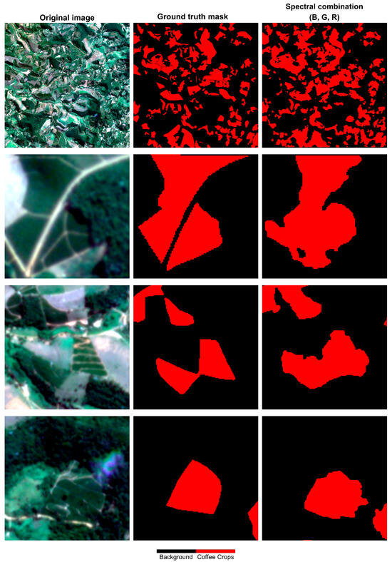
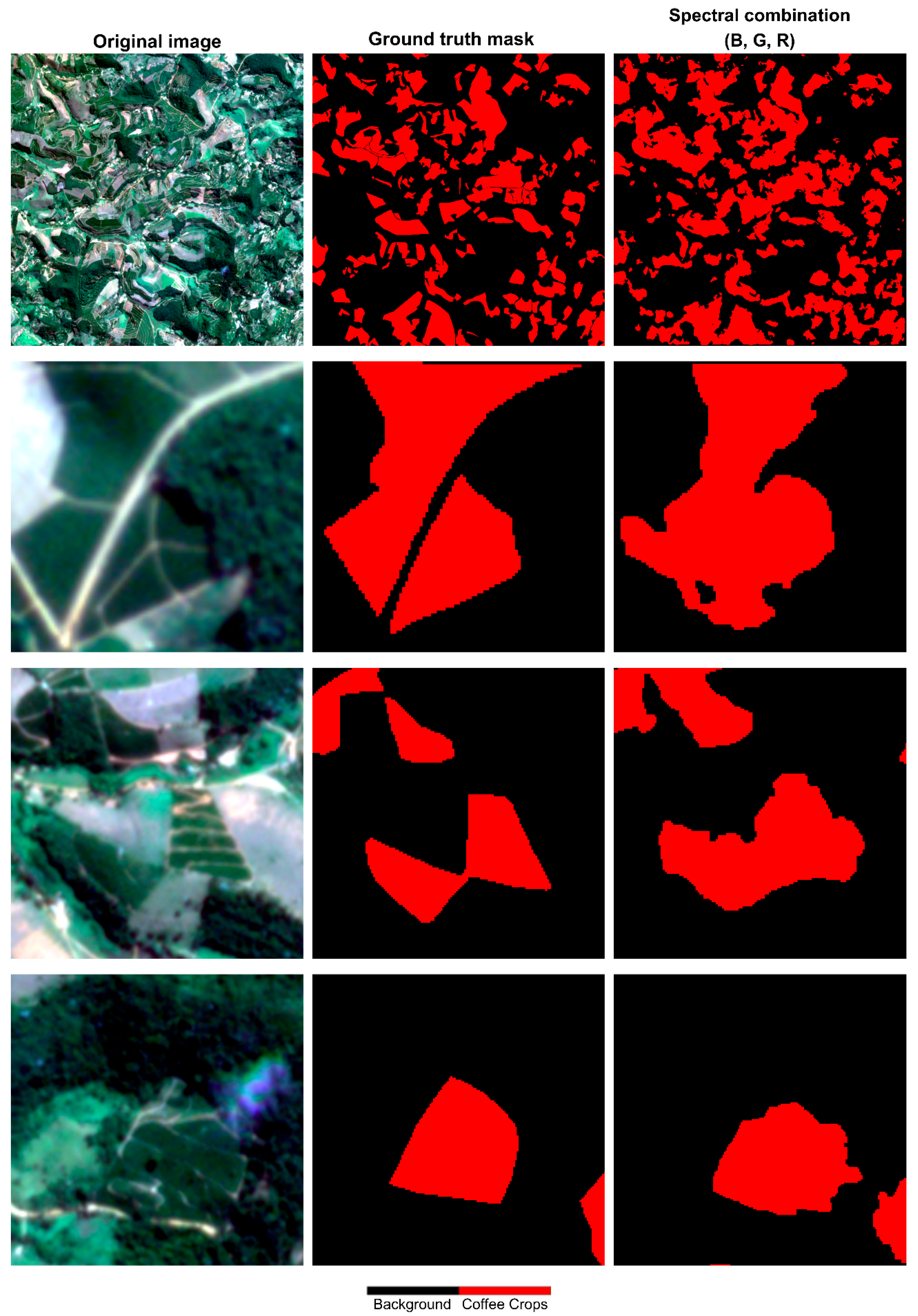
In addition to analyzing quantitative and qualitative results, the total predicted area for the Coffee Crops class in the test scene was evaluated. The actual area manually labeled for the Coffee Crops class in the test scene was 1002.123 hectares. The areas predicted by the U-Net model for each combination were: 1185.614 hectares for (B, G, R), 1224.710 hectares for (B, G, R, NIR), 1251.150 hectares for (G, R, NIR), 1301.850 hectares for (B, R, NIR), and 1525.110 hectares for (B, G, NIR). These results show that the (B, G, R) combination produced the smallest overestimation, approximately 183.491 hectares (18.3%), while the remaining combinations yielded progressively larger overestimations. This overestimation pattern across all combinations demonstrates the model’s difficulty in defining precise plot boundaries, reflecting the occurrence of False Positives (FP). To better understand this behavior in spatial terms, Figure 5 presents the full prediction for scene 3, comprising the original image, ground truth mask, and enlargements of selected Coffee Crops plots and prediction obtained using the combination (B, G, R).

Figure 5. The first row shows the complete PlanetScope (B, G, R) image, the corresponding ground truth mask, and the predicted segmentation. The lower rows present zoom-in views of selected coffee plantation plots. Colors indicate Coffee Crops (red) and Background (black) classes.

4. Discussion

4.1. Superior Performance of Visible Bands in Coffee Segmentation

Results obtained in this study demonstrate that the visible spectrum band combination (B, G, R) was the most efficient for coffee crop segmentation, presenting the highest Accuracy and IoU values among evaluated configurations (Table 2 and Table 3). Although NIR is traditionally associated with vegetation discrimination [35], its inclusion in evaluated combinations did not result in performance improvement, suggesting that, in this context, visible spectral information was more relevant for differentiating coffee crops from their surroundings. This finding reinforces the need to analyze band choice contextually, considering both the crop’s spectral response and the environmental and topographic conditions of the study area.

The spectral separability analysis provides quantitative evidence supporting these findings. Absolute Jeffries-Matusita (JM) distances, which measure the statistical distance between two classes, were modest (0.27 to 0.44 on a 0 to 2 scale). This modesty reflects how difficult it is to distinguish coffee from vegetated backgrounds in mountainous landscapes. However, visible spectral bands (Blue, Green, and Red) showed a strong relative advantage over the Near-Infrared (NIR) band: Blue, Green, and Red achieved 43% to 62% higher separability than NIR. This result may seem paradoxical. While NIR exhibited the largest mean difference between classes (Δ = 0.046), it had the lowest separability (JM = 0.274). This is due to high spectral variance (standard deviation, SD) within both classes. In Matas de Minas, coffee plantations coexist with native Atlantic Forest vegetation. Both exhibit strong NIR responses due to healthy leaf cellular structure. The resulting spectral overlap (SD ≈ 0.08 in NIR for both classes) confounds pixel-level discrimination, despite differences in mean values.

This behavior can be attributed to the spectral and plant-architecture characteristics of the coffee crop, which include dense crowns, pronounced internal shading, and an irregular canopy shape. Additionally, the large number of cultivated varieties and diverse plant stands contribute to increased spectral heterogeneity within coffee plantations. Such characteristics reduce the typical high reflectance response in NIR, frequently observed in annual and homogeneous crops. In contrast, color and brightness variations in leaves, mainly in red and green bands, more clearly express differences in vegetative vigor, phenological stage, and foliar density among plots [34]. Thus, the greater sensitivity of the visible spectrum to pigmentation variations becomes fundamental for distinguishing coffee areas in complex, heterogeneous environments, such as Matas de Minas. Furthermore, visible bands capture differences in canopy pigmentation, internal shadowing, and foliar density with lower within-class variance, resulting in better spectral discrimination despite smaller absolute differences between class means.

From a methodological perspective, adding extra bands may have caused spectral redundancy and increased the dimensionality of the feature space, which tends to increase noise and reduce the network’s generalization capacity. This phenomenon was also reported by [33], who highlight that optimal band selection depends directly on the type of cover analyzed and geographical context, and that indiscriminate addition of bands can harm learning in deep learning-based models. In the case of the U-Net architecture, whose convolutional structure is designed to explore spatial and semantic patterns, the information contained in the visible spectrum proved sufficient to capture relevant contrasts between crops and other covers. Moreover, NIR introduced more spectral confusion, especially in areas with native vegetation and crop edges. The separability analysis quantitatively confirms this observation: the minimum JM within a band combination determines its weakest discriminative component (Table 4). (B, G, R) maintained a minimum JM of 0.391, while all NIR-inclusive combinations dropped to a minimum JM of 0.274, representing a reduction solely due to NIR inclusion. This weak link effect explains why adding NIR to (B, G, R) led to a performance decline across all metrics (Table 3), with IoU decreasing from 0.7671 to 0.7356. The modest absolute JM values do not contradict the model’s performance (F1-score of 0.87, IoU of 0.77), as the U-Net leverages spatial context and multi-scale features beyond pixel-level spectral differences.

From a practical standpoint, these results indicate that sensors with visible spectrum can be adequate for mapping coffee crops. This is especially true in mountainous and heterogeneous regions, where the use of multispectral sensors implies higher costs and greater operational complexity. The good performance of visible spectrum bands highlights the viability of lower-cost images without significant loss of accuracy. This represents a substantial advancement for precision agriculture and the remote monitoring of permanent crops. Additionally, reducing investment in data acquisition expands the potential use of deep neural networks in diverse operational and regional contexts.

Therefore, the results reinforce that the efficiency of coffee crop segmentation is related to the spectral composition of the input images. The visible spectrum proved to be the most informative for discriminating coffee areas, balancing spectral contrast and geometric consistency. The incorporation of additional bands, such as NIR, did not yield significant gains and, in some cases, compromised the spatial and semantic precision of segmentations. These findings confirm the importance of spectral band selection, considering both the physical properties of the canopy and the specific characteristics of the deep learning models used in digital agriculture.

Compared with the state of the art in satellite-based coffee mapping, the results of this study are consistent with performance levels reported in the literature, despite methodological differences. Parreiras et al. [24] achieved high detection accuracy using dense Landsat Sentinel-2 time series and machine learning, but their approach depends on extensive multitemporal data, auxiliary variables, and pixel-based classification, and was validated in a single, relatively homogeneous municipality. Kebede et al. [23] reported 89.9% overall accuracy using a two-step pixel and sub-pixel framework; however, the initial stage showed low accuracy for coffee cropland (PA = 59.4%) and relied on multiple auxiliary datasets, limiting operational replicability. Maskell et al. [14] obtained 89% binary accuracy by fusing Sentinel-1 and Sentinel-2 data, at the cost of increased data requirements and methodological complexity. In contrast, the present study demonstrates that comparable segmentation performance can be achieved with a single high-resolution optical sensor and a standard U-Net architecture, and that visible bands alone are sufficient for coffee segmentation in mountainous and heterogeneous environments.

4.2. Impact of Resolution and Discrepancy Between F1-Score and IoU

The discrepancy observed between F1-score and IoU values in this study reflects conceptual aspects of evaluation metrics and inherent limitations of the spatial resolution of images used. For the Coffee Crops class, the model with combination (B, G, R) achieved an F1-score of 0.8682, but a considerably lower IoU of 0.7671. This difference is expected, since the F1-score, being a harmonic mean between Precision and Recall, is more tolerant to variations in edges and small contour deviations. IoU, on the other hand, more severely penalizes spatial discrepancies, since it incorporates in the denominator the sum of False Positives (FP) and False Negatives (FN). Thus, models that correctly capture the general location of crops may still exhibit a reduced IoU if segmented boundaries do not perfectly coincide with actual limits, a behavior already described in agricultural segmentation studies using Deep Learning [21,29].

This difficulty in defining plot boundaries is quantified by evaluating the total predicted area for the Coffee Crops class using a combination of (B, G, R), which overestimates the cultivated area by approximately 183.491 hectares, representing 18.3% more than the actual cultivated coffee area.

The observed overestimation is not merely a random error but indicates a systematic positive bias driven by the interaction between the sensor’s spatial resolution and the U-Net’s inductive bias. Quantitatively, this is evidenced in Table 3, where Recall (0.8769) exceeds Precision (0.8596) for the (B, G, R) configuration. This indicates that the model favors inclusion over exclusion at decision boundaries, generating more False Positives than False Negatives and thus producing a predicted mask spatially larger than the ground truth. Methodologically, the U-Net architecture, which relies on convolutional filters to aggregate spatial and spectral context, tends to propagate the strong spectral signal of the coffee canopy into transition pixels that contain a mixture of crop and background. Consequently, the model effectively dilates crop boundaries by classifying the mixed transition belt as the positive class, leading to cumulative area overestimation.

This boundary effect is well documented in the literature. Several studies have highlighted that mixed pixels are among the factors that most negatively affect efficiency in land use and land cover classifications, especially in tropical mountainous areas, where topographic effects accentuate spectral variability [18,44]. Although the 4 m spatial resolution of PlanetScope reduces this problem compared to medium-resolution sensors such as Landsat, it remains insufficient to eliminate spectral confusion at plot edges in fragmented landscapes such as Matas de Minas. Consequently, the results indicate that a high F1-score reflects the model’s ability to detect the class, while a lower IoU evidences limitations in precise boundary definition, which are directly associated with the mixed-pixel mechanism described above.

4.3. Limitations and Future Work

The results of this study are consistent and well-supported for the Matas de Minas region, characterized by mountainous terrain, Arabica coffee cultivation, and coexistence with native Atlantic Forest vegetation. Because the spectral relationship between coffee and its surrounding land covers may vary across regions with different topography, coffee species, or vegetation, validating the proposed approach in other producing areas is a natural extension of this research.

The evaluation strategy adopted a single spatially independent scene as the test set, ensuring strict spatial separation between training and test data and preventing inflated performance estimates due to spatial autocorrelation. To strengthen these conclusions, future studies could use a leave-one-scene-out cross-validation strategy to expand assessment of band-combination performance across diverse landscapes. Data augmentation techniques were not applied to isolate the effect of spectral band combinations without confounding variables. Including augmentation strategies in future work could improve model performance and test if the observed band ranking remains stable with expanded training.

Future work should focus on three main directions: expanding the dataset by adding more scenes and annotations for the coffee crop (including different phenological stages and acquisition conditions), evaluating the proposed approach in coffee-producing regions with varying environmental and management conditions, and adopting advanced validation strategies. This includes multi-scene cross-validation, data augmentation, and the exploration of alternative spectral or explainability analyses, all to robustly test the applicability and generalizability of the findings.

5. Conclusions

This study evaluated the impact of different PlanetScope sensor spectral band combinations on the performance of the U-Net architecture applied to the semantic segmentation of coffee crops in Matas de Minas. Results confirmed the hypothesis that, in perennial crops with complex canopies, such as coffee, visible spectrum bands (B, G, R) are more effective for segmenting cultivated areas than combinations that include near-infrared (NIR) bands. This finding was independently supported by the Jeffries-Matusita separability analysis, which demonstrated that visible bands achieved 43% to 62% higher spectral discrimination than NIR, whose high within-class variance reduced its capacity to distinguish coffee from surrounding vegetation. Although the visible combination presented the best performance, the model demonstrated limitations in delimiting coffee cultivated area boundaries. This challenge was amplified by the occurrence of mixed pixels associated with image spatial resolution and study region characteristics, characterized by mountainous relief and fragmented agricultural cover, resulting in an overestimation of the cultivated area. These findings reinforce the importance of contextualized approaches in selecting input bands for deep learning models, but also expose the need for data that allows better spatial delimitation. As future perspectives, it is recommended to validate the method in other producing regions under different topographic and spectral conditions. Additionally, investigating the integration of optical and radar data, as well as the use of images with higher spatial resolution, aims to improve plot delimitation and increase model generalization.

References

- Spence, C.; Carvalho, F.M. The Coffee Drinking Experience: Product Extrinsic (Atmospheric) Influences on Taste and Choice. Food Qual. Prefer. 2020, 80, 103802. [Google Scholar] [CrossRef] [Scilit]
- FAO. Global Coffee Market and Recent Price Developments; FAO: Rome, Italy, 2025. [Google Scholar]
- DaMatta, F.M.; Rahn, E.; Läderach, P.; Ghini, R.; Ramalho, J.C. Why Could the Coffee Crop Endure Climate Change and Global Warming to a Greater Extent than Previously Estimated? Clim. Change 2019, 152, 167–178. [Google Scholar] [CrossRef] [Scilit]
- ICO. Coffee Development Report; ICO: London, UK, 2023. [Google Scholar]
- Bolaños, J.; Corrales, J.C.; Campo, L.V. Feasibility of Early Yield Prediction per Coffee Tree Based on Multispectral Aerial Imagery: Case of Arabica Coffee Crops in Cauca-Colombia. Remote Sens. 2023, 15, 282. [Google Scholar] [CrossRef] [Scilit]
- Jabed, M.A.; Azmi Murad, M.A. Crop Yield Prediction in Agriculture: A Comprehensive Review of Machine Learning and Deep Learning Approaches, with Insights for Future Research and Sustainability. Heliyon 2024, 10, e40836. [Google Scholar] [CrossRef] [Scilit]
- Kouadio, L.; Byrareddy, V.M.; Sawadogo, A.; Newlands, N.K. Probabilistic Yield Forecasting of Robusta Coffee at the Farm Scale Using Agroclimatic and Remote Sensing Derived Indices. Agric. For. Meteorol. 2021, 306, 108449. [Google Scholar] [CrossRef] [Scilit]
- Hunt, D.A.; Tabor, K.; Hewson, J.H.; Wood, M.A.; Reymondin, L.; Koenig, K.; Schmitt-Harsh, M.; Follett, F. Review of Remote Sensing Methods to Map Coffee Production Systems. Remote Sens. 2020, 12, 2041. [Google Scholar] [CrossRef] [Scilit]
- Nogueira Martins, R.; de Assis de Carvalho Pinto, F.; Marçal de Queiroz, D.; Sárvio Magalhães Valente, D.; Tadeu Fim Rosas, J.; Fagundes Portes, M.; Sânzio Aguiar Cerqueira, E. Digital Mapping of Coffee Ripeness Using UAV-Based Multispectral Imagery. Comput. Electron. Agric. 2023, 204, 107499. [Google Scholar] [CrossRef] [Scilit]
- Martínez-Verduzco, G.C.; Galeana-Pizaña, J.M.; Cruz-Bello, G.M. Coupling Community Mapping and Supervised Classification to Discriminate Shade Coffee from Natural Vegetation. Appl. Geogr. 2012, 34, 1–9. [Google Scholar] [CrossRef] [Scilit]
- Moreira, M.A.; Barros, M.A.; Rudorff, B.F.T. Geotechnologies in Coffee Crop Mapping at Municipality Scale. Soc. Nat. 2008, 20, 101–110. [Google Scholar] [CrossRef] [Scilit]
- Bourgoin, C.; Oszwald, J.; Bourgoin, J.; Gond, V.; Blanc, L.; Dessard, H.; Van Phan, T.; Sist, P.; Läderach, P.; Reymondin, L. Assessing the Ecological Vulnerability of Forest Landscape to Agricultural Frontier Expansion in the Central Highlands of Vietnam. Int. J. Appl. Earth Obs. Geoinf. 2020, 84, 101958. [Google Scholar] [CrossRef] [Scilit]
- Pereira, F.V.; Orlando, V.S.W.; Martins, G.D.; Vieira, B.S.; Nascimento, E.S.; Marra, A.B.; de Lourdes Bueno Trindade Galo, M. Estimating Coffee Crop Parameters through Multispectral Imaging and Machine Learning Algorithms. ISPRS Ann. Photogramm. Remote Sens. Spat. Inf. Sci. 2024, X-3–2024, 317–323. [Google Scholar] [CrossRef] [Scilit]
- Maskell, G.; Chemura, A.; Nguyen, H.; Gornott, C.; Mondal, P. Integration of Sentinel Optical and Radar Data for Mapping Smallholder Coffee Production Systems in Vietnam. Remote Sens. Environ. 2021, 266, 112709. [Google Scholar] [CrossRef] [Scilit]
- Oviedo, A.D.; Pencue-Fierro, E.L.; Muñoz, J.F.; Solano-Correa, Y.T. Coffee Trees Segmentation in UAV-Acquired Images Using Deep Learning. In Proceedings of the 2024 18th National Meeting on Optics and the 9th Andean and Caribbean Conference on Optics and Its Applications, ENO-CANCOA 2024—Conference Proceedings, Cartagena, Colombia, 12–14 June 2024. [Google Scholar] [CrossRef] [Scilit]
- Arriola-Valverde, S.; Rimolo-Donadio, R.; Villagra-Mendoza, K.; Chacón-Rodriguez, A.; García-Ramirez, R.; Somarriba-Chavez, E. A Comparative Study of Deep Learning Frameworks Applied to Coffee Plant Detection from Close-Range UAS-RGB Imagery in Costa Rica. Remote Sens. 2024, 16, 4617. [Google Scholar] [CrossRef] [Scilit]
- Le, Q.T.; Dang, K.B.; Giang, T.L.; Tong, T.H.A.; Nguyen, V.G.; Nguyen, T.D.L.; Yasir, M. Deep Learning Model Development for Detecting Coffee Tree Changes Based on Sentinel-2 Imagery in Vietnam. IEEE Access 2022, 10, 109097–109107. [Google Scholar] [CrossRef] [Scilit]
- de Carvalho Alves, M.; Sanches, L.; Silva de Menezes, F.; Trindade, L.R.S.L.C. Multisensor Analysis for Environmental Targets Identification in the Region of Funil Dam, State of Minas Gerais, Brazil. Appl. Geomat. 2023, 15, 807–827. [Google Scholar] [CrossRef] [Scilit]
- Schmitt-Harsh, M. Landscape Change in Guatemala: Driving Forces of Forest and Coffee Agroforest Expansion and Contraction from 1990 to 2010. Appl. Geogr. 2013, 40, 40–50. [Google Scholar] [CrossRef] [Scilit]
- Wang, H.; Hu, C.; Zhang, R.; Qian, W. SegForest: A Segmentation Model for Remote Sensing Images. Forests 2023, 14, 1509. [Google Scholar] [CrossRef] [Scilit]
- Chang, Z.; Li, H.; Chen, D.; Liu, Y.; Zou, C.; Chen, J.; Han, W.; Liu, S.; Zhang, N. Crop Type Identification Using High-Resolution Remote Sensing Images Based on an Improved DeepLabV3+ Network. Remote Sens. 2023, 15, 5088. [Google Scholar] [CrossRef] [Scilit]
- Zangana, H.M.; Li, S.; Wani, S. Diffusion Models for Agricultural Imaging: A Systematic Review of Methods, Applications and Future Prospects. Impact Agric. 2025, 1, 1–11. [Google Scholar] [CrossRef] [Scilit]
- Kebede, G.; Mudereri, B.T.; Mutanga, O.; Landmann, T.; Odindi, J.; Motisi, N.; Pinard, F.; Tonnang, H.E.Z.; Abdel-Rahman, E.M. Mapping Robusta Coffee (Coffea canephora) Cropping Systems in Uganda: A Two-Step Pixel and Sub-Pixel Based Approach with Sentinel-2 Data. PLoS ONE 2026, 21, e0338803. [Google Scholar] [CrossRef] [Scilit]
- Parreiras, T.C.; Santos, C.d.O.; Bolfe, É.L.; Sano, E.E.; Leandro, V.B.S.; Bayma, G.; da Silva, L.A.P.; Furuya, D.E.G.; Romani, L.A.S.; Morton, D. Dense Time Series of Harmonized Landsat Sentinel-2 and Ensemble Machine Learning to Map Coffee Production Stages. Remote Sens. 2025, 17, 3168. [Google Scholar] [CrossRef] [Scilit]
- Ayhan, B.; Kwan, C.; Budavari, B.; Kwan, L.; Lu, Y.; Perez, D.; Li, J.; Skarlatos, D.; Vlachos, M. Vegetation Detection Using Deep Learning and Conventional Methods. Remote Sens. 2020, 12, 2502. [Google Scholar] [CrossRef] [Scilit]
- Gonthina, N.; Narasimha Prasad, L.V. An Enhanced Convolutional Neural Network Architecture for Semantic Segmentation in High-Resolution Remote Sensing Images. Discov. Comput. 2025, 28, 91. [Google Scholar] [CrossRef] [Scilit]
- Luo, Z.; Pan, J.; Hu, Y.; Deng, L.; Li, Y.; Qi, C.; Wang, X. RS-Dseg: Semantic Segmentation of High-Resolution Remote Sensing Images Based on a Diffusion Model Component with Unsupervised Pretraining. Sci. Rep. 2024, 14, 18609. [Google Scholar] [CrossRef] [Scilit]
- Song, W.; He, H.; Dai, J.; Jia, G. Spatially Adaptive Interaction Network for Semantic Segmentation of High-Resolution Remote Sensing Images. Sci. Rep. 2025, 15, 15337. [Google Scholar] [CrossRef] [Scilit] [PubMed]
- Zhang, X.; Han, L.; Han, L.; Zhu, L. How Well Do Deep Learning-Based Methods for Land Cover Classification and Object Detection Perform on High Resolution Remote Sensing Imagery? Remote Sens. 2020, 12, 417. [Google Scholar] [CrossRef] [Scilit]
- Ronneberger, O.; Fischer, P.; Brox, T. U-Net: Convolutional Networks for Biomedical Image Segmentation. In Medical Image Computing and Computer-Assisted Intervention—MICCAI 2015; Lecture Notes in Computer Science; Springer: Berlin/Heidelberg, Germany, 2015; Volume 9351, pp. 234–241. [Google Scholar] [CrossRef] [Scilit]
- Altan, O.; Huang, M.; Xiao, C.; Chen, N.; Li, R.; Dimitrovski, I.; Spasev, V.; Loshkovska, S.; Kitanovski, I. U-Net Ensemble for Enhanced Semantic Segmentation in Remote Sensing Imagery. Remote Sens. 2024, 16, 2077. [Google Scholar] [CrossRef] [Scilit]
- Ji, Z.; Xu, J.; Yan, L.; Ma, J.; Chen, B.; Zhang, Y.; Zhang, L.; Wang, P. Satellite Remote Sensing Images of Crown Segmentation and Forest Inventory Based on BlendMask. Forests 2024, 15, 1320. [Google Scholar] [CrossRef] [Scilit]
- Bhuiyan, M.A.E.; Witharana, C.; Liljedahl, A.K.; Jones, B.M.; Daanen, R.; Epstein, H.E.; Kent, K.; Griffin, C.G.; Agnew, A. Understanding the Effects of Optimal Combination of Spectral Bands on Deep Learning Model Predictions: A Case Study Based on Permafrost Tundra Landform Mapping Using High Resolution Multispectral Satellite Imagery. J. Imaging 2020, 6, 97. [Google Scholar] [CrossRef] [Scilit]
- Ding, B.; Tian, J.; Wang, Y.; Zeng, T. Land Cover Extraction in the Typical Black Soil Region of Northeast China Using High-Resolution Remote Sensing Imagery. Land 2023, 12, 1566. [Google Scholar] [CrossRef] [Scilit]
- Hatfield, J.L.; Prueger, J.H.; Sauer, T.J.; Dold, C.; O’brien, P.; Wacha, K. Applications of Vegetative Indices from Remote Sensing to Agriculture: Past and Future. Inventions 2019, 4, 71. [Google Scholar] [CrossRef] [Scilit]
- Jia, P.; Chen, C.; Zhang, D.; Sang, Y.; Zhang, L. Semantic Segmentation of Deep Learning Remote Sensing Images Based on Band Combination Principle: Application in Urban Planning and Land Use. Comput. Commun. 2024, 217, 97–106. [Google Scholar] [CrossRef] [Scilit]
- Roy, D.P.; Huang, H.; Houborg, R.; Martins, V.S. A Global Analysis of the Temporal Availability of PlanetScope High Spatial Resolution Multi-Spectral Imagery. Remote Sens. Environ. 2021, 264, 112586. [Google Scholar] [CrossRef] [Scilit]
- INPI. Ficha Técnica de Registro de Indicação Geográfica; Instituto Nacional da Propriedade Industrial: Rio de Janeiro, Brazil, 2020. [Google Scholar]
- QGIS Development Team. QGIS Geographic Information System; QGIS Development Team: Zürich, Switzerland, 2021. [Google Scholar]
- Karasiak, N.; Dejoux, J.F.; Monteil, C.; Sheeren, D. Spatial Dependence between Training and Test Sets: Another Pitfall of Classification Accuracy Assessment in Remote Sensing. Mach. Learn. 2021, 111, 2715–2740. [Google Scholar] [CrossRef] [Scilit]
- Griffith, D.A.; Chun, Y. Spatial Autocorrelation and Uncertainty Associated with Remotely-Sensed Data. Remote Sens. 2016, 8, 535. [Google Scholar] [CrossRef] [Scilit]
- Kattenborn, T.; Schiefer, F.; Frey, J.; Feilhauer, H.; Mahecha, M.D.; Dormann, C.F. Spatially Autocorrelated Training and Validation Samples Inflate Performance Assessment of Convolutional Neural Networks. ISPRS Open J. Photogramm. Remote Sens. 2022, 5, 100018. [Google Scholar] [CrossRef] [Scilit]
- Richards, J.; Jia, X. Remote Sensing Digital Image Analysis: An Introduction; Springer: Berlin/Heidelberg, Germany, 2006. [Google Scholar]
- Tong, X.Y.; Xia, G.S.; Zhu, X.X. Enabling Country-Scale Land Cover Mapping with Meter-Resolution Satellite Imagery. ISPRS J. Photogramm. Remote Sens. 2023, 196, 178–196. [Google Scholar] [CrossRef] [Scilit]
Disclaimer/Publisher’s Note: The statements, opinions and data contained in all publications are solely those of the individual author(s) and contributor(s) and not of MDPI and/or the editor(s). MDPI and/or the editor(s) disclaim responsibility for any injury to people or property resulting from any ideas, methods, instructions or products referred to in the content. |
© 2026 by the authors. Licensee MDPI, Basel, Switzerland. This article is an open access article distributed under the terms and conditions of the Creative Commons Attribution (CC BY) license.