


Abstract
Path planning for rice-seedling-throwing machines (RSTMs) remains a challenging task in karst areas, where paddy fields are typically small, fragmented, and bounded by irregular, tortuous boundaries. This study integrates an adaptive model of headland turning costs with an improved pelican optimization algorithm (IPOA). Using the minimum turning radius and field boundaries, a turning cost function covering X- and U-type turns is established, with a dimensionless composite performance index defined as a weighted sum of operation time and fuel consumption. Two strategies are added: a Lévy flight disturbance to escape local optima and strengthen global exploration, and a nonlinear convergence factor that replaces the linear decay and supports early global exploration and later fine local exploitation. The model is coupled with the optimizer to convert boundary constraints into feasible turns and embed turning costs into row sequencing. Across ten fields and 30 independent runs, the improved POA, termed IPOA, attains the lowest mean path length, operation time, fuel consumption, and composite index C, reducing the composite index C by 4.46%, 2.44%, 1.72%, and 1.48% on average relative to the genetic algorithm (GA), ant colony optimization (ACO), particle swarm optimization (PSO), and POA. The lower mean values and the statistical evidence are kept distinct: Wilcoxon and Friedman tests confirm that the overall ranking advantage is statistically significant, offering a transferable route to energy-efficient precision agriculture in karst areas.
1. Introduction
Guangxi has a complex terrain, and more than 59% of its land is covered by karst [1]. These extensive karst landforms aggravate the spatial heterogeneity and ecological vulnerability of cultivated land [2]. Under the combined influence of natural conditions and human activities, farmland in this region is highly fragmented into small, scattered, and irregularly shaped patches [3]. Fragmentation is particularly severe in the karst areas of Guangxi, where redundant field ridges waste 5–10% of the cultivated land and large-scale mechanization remains difficult [4]. The terrain also undulates strongly and slopes change abruptly, increasing the difficulty and safety risk of machinery operations [5]. Relying on driver experience or fixed operation modes therefore leads to repeated coverage, missed areas, and elevated risk on steep slopes, reducing efficiency and output quality while increasing fuel consumption and machine wear. Optimizing operation paths for this terrain is therefore essential for overcoming a bottleneck in local agricultural mechanization and for supporting food security.
Autonomous navigation and path planning for agricultural machinery have advanced rapidly, covering sensor integration, core algorithms, and motion control. Hossain et al. [6] assessed the integration of GPS, machine learning, and sensors for automatic navigation and identified technical and infrastructural barriers. Wu [7] reviewed autonomous field navigation and concluded that unstructured farmland, variable terrain, and the need for robust adaptive control remain the main bottlenecks, calling for terrain-aware planning that accommodates irregular boundaries and elevation changes. Zhang et al. [8] reviewed path-tracking models and noted that non-flat terrain, wheel slip, and dynamic disturbances still limit tracking accuracy. At the planning level, Xu et al. [9] used UAV imagery to locate fruit trees and planting rows and planned paths for ground vehicles and UAVs, while Han et al. [10] developed a field path planner with an X-type turning mode for polygonal paddy fields and validated it on an autonomous tractor. These studies nonetheless assume largely regular boundaries and flat terrain, and their methods do not transfer directly to the fragmented, highly irregular farmland of the karst areas of Guangxi.
To address these limitations, several studies have extended planning to hilly and irregular fields. Jiang and Yang [11] formulated three-dimensional coverage planning with a movement-energy cost for robots on non-flat ground. Li et al. [12] combined oblique photography with global three-dimensional planning and validated it in a hilly tea garden. Yang [13] planned paths for a seeding robot on small irregular terraces, using Bézier fitting to smooth the boundary-wrapping path. Ni et al. [14] proposed a hybrid coverage planner based on an improved Reeds–Shepp curve to reduce the space required by conventional U-turns at non-perpendicular boundaries, thereby narrowing the reserved headland and shortening the non-working path. Kuang et al. [15] cast coverage planning as a traveling salesman problem and solved it with Monte Carlo reinforcement learning in a multi-objective framework (CPP-DIP). These studies, however, concentrate on geometric path generation and local turn adjustment; the global order of row traversal is still set by fixed rules or simplified assumptions and does not capture the trade-off between operation time and fuel consumption.
Because global traversal-order optimization is a combinatorial problem, recent work has increasingly applied metaheuristics. The genetic algorithm (GA) remains a standard choice but requires many iterations to produce feasible solutions and is computationally inefficient [16]. Particle swarm optimization (PSO) searches effectively yet converges slowly and is prone to local optima [17]. Ant colony optimization (ACO) offers path diversity and global search but suffers from weak initial guidance, slow convergence, and redundant inflection points [18]. The whale optimization algorithm (WOA) converges quickly and accurately but loses population diversity [19], whereas the Harris hawks optimization (HHO) improves path accuracy and convergence through circle-map initialization yet remains sensitive to initialization [20]. Liu et al. [21] applied an enhanced gray wolf optimizer (GWO) to UAV trajectory planning in hilly terrain and confirmed its adaptability.
These studies confirm the potential of metaheuristics but also expose their shared weaknesses—slow convergence, limited population diversity, and entrapment in local optima—which are amplified in the highly constrained, nonlinear planning space of karst farmland. A suitable algorithm should therefore combine a simple structure, strong global search, and straightforward multi-strategy improvement. The pelican optimization algorithm (POA), proposed by Trojovský and Dehghani [22], meets the first two requirements: it mimics pelican hunting through distinct exploration and exploitation stages. Its standard form, however, converges slowly in later iterations and can stagnate at local optima. Recent variants have introduced three-dimensional spiral flight, Lévy flight, and chaotic mapping and have been validated on benchmark and UAV-planning tasks [23,24,25,26], but these improvements target general optimization problems rather than the combined time–fuel penalty caused by frequent, non-standard turns in karst farmland. Designing a planner that adapts its traversal strategy to boundary constraints while maintaining efficient search therefore remains an open problem.
Existing work has advanced coverage-path generation, turning-cost modeling, and metaheuristic optimization, and this study builds on two established elements: geometric turning models and POA variants with Lévy flight and nonlinear convergence. Three differences remain. First, most turning models [11,12,13,14,15] rely on fixed rules or local geometric adjustment and optimize path length or operation time under relatively regular boundaries, whereas the present model selects X- or U-type turns from the inter-row spacing, embeds the minimum turning radius R and the local boundary inclination θ1, and quantifies both operation time and fuel consumption on irregular boundaries. Second, existing POA variants [23,24,25,26] apply Lévy flight, chaotic mapping, or spiral search mainly to benchmark functions and UAV planning, without coupling the operators to agricultural turning constraints; here the turning-cost model serves directly as the fitness function, so the optimizer searches the row traversal sequence under the composite index C. Third, earlier studies treat turning-path generation and global row sequencing separately, whereas this work couples them by converting boundary constraints into feasible turns and embedding turning penalties in the sequence search. The novelty therefore lies not in the individual operators but in this problem-specific coupling for RSTMs in fragmented karst paddy fields.
The main contributions are as follows. (1) A boundary-adaptive coverage-planning framework for irregular karst paddy fields, integrating headland turning-cost quantification with traversal-sequence optimization and providing a dedicated solution for rice-seedling-throwing operations on small, fragmented plots. (2) A headland turning-cost model. Two kinematically defined turning patterns are selected by a row-spacing feasibility threshold, with local boundary angles embedded in the path geometry. A unified metric combining dimensionless operation time and simulated fuel consumption yields a reliable single-turn cost for irregular field configurations. (3) Composite-index-driven sequence optimization. The IPOA with Lévy-flight perturbation and a nonlinear convergence factor is coupled with ROV decoding, which converts continuous search vectors into feasible row permutations to minimize the composite index C globally. The remainder of this paper is organized as follows: Section 2 develops the turning patterns and the IPOA, Section 3 presents the case study, and Section 4 concludes the paper.
2. Method Proposal
2.1. X- and U-Type Turning Patterns in Irregularly Shaped Fields
The ultimate goal of path planning is to determine the optimal traversal order of a set of operation rows such that the composite index C incurred by the agricultural machinery in completing all seeding operations is minimized. The dominant component of this cost comprises the time cost and fuel consumption arising from the turning maneuvers performed when the machine transfers between successive operation rows. Accordingly, constructing a mathematical model that can accurately characterize the costs of different turning maneuvers is a prerequisite for the subsequent path optimization. First, the basic operating parameters of the machine are presented; then, the path length, time, and fuel consumption of two typical turning modes are derived; and finally, a unified composite index C evaluation model is established on this basis [27].
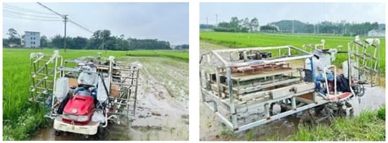
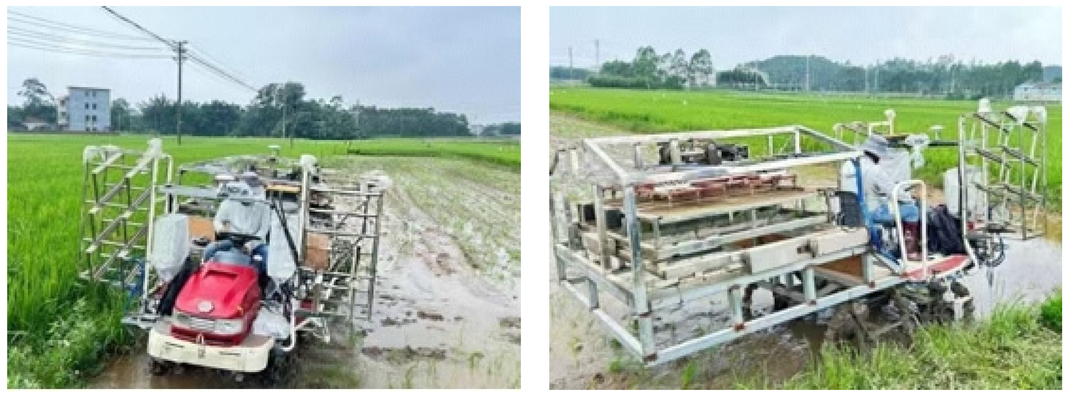
In this study, RSTMs manufactured by a company in Guangxi and shown in Figure 1 are used as the research object. The overall width of the machine is 1.9 m, and the single working width of the matched seedling-throwing mechanism is equal to this; accordingly, the width of each operation row is set to 2 m. The designed minimum turning radius of the machine is 3.1 m. Because the actual travel path of the machine is represented in this study by the trajectory of its geometric center, when the machine turns at its minimum turning radius, the turning radius of this center trajectory is given by the following:
Figure 1.
Self-developed RSTM prototype.
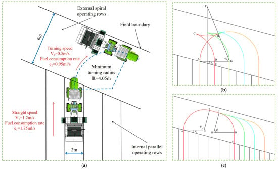
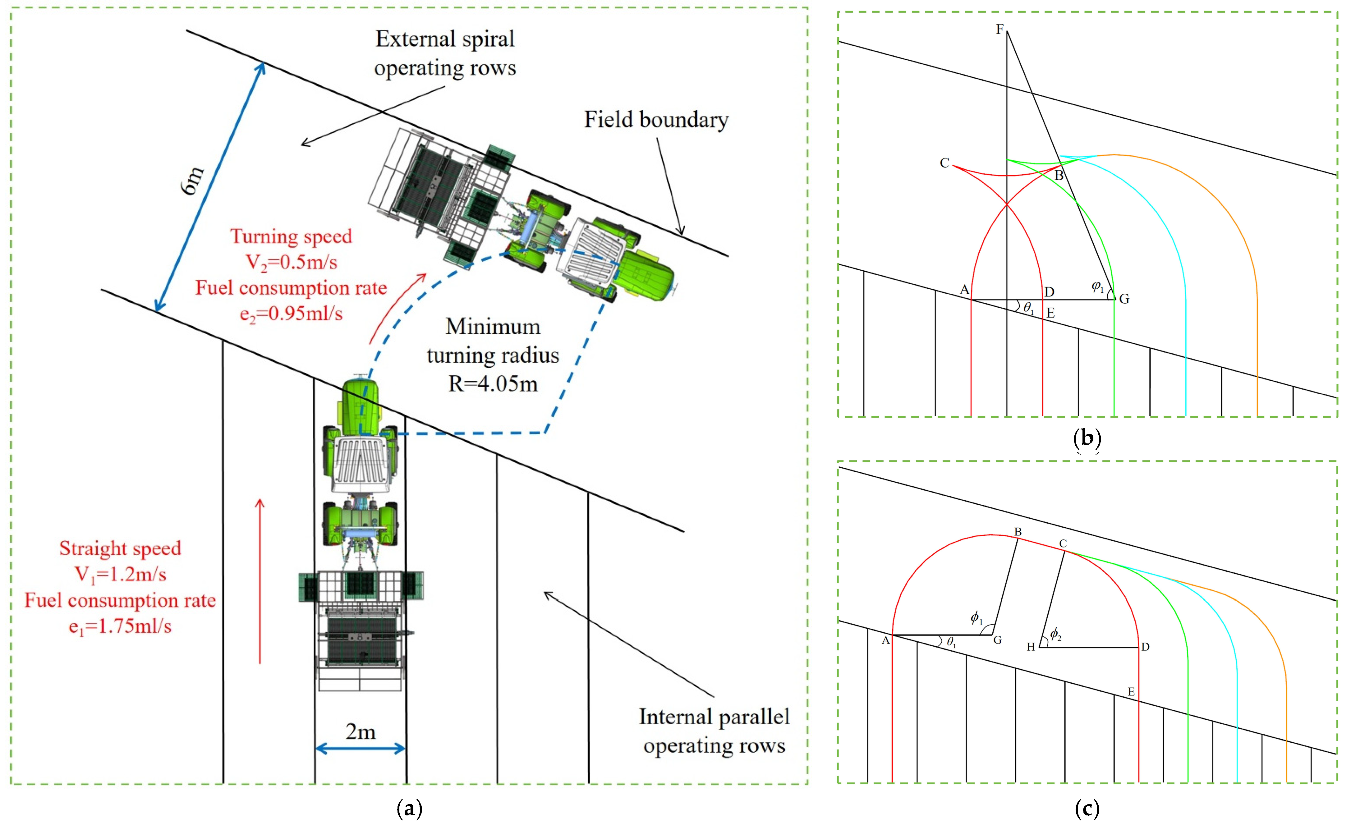
This value is denoted as R and serves as the basic parameter for the subsequent geometric derivation of the turning paths. During normal seeding operations, the machine travels at a constant speed of V1 = 1.2 m/s to ensure seeding quality and efficiency, with a corresponding fuel consumption rate of e1 = 1.75 ml/s. When the machine performs a turning maneuver at the minimum turning radius, its travel speed is reduced to V2 = 0.5 m/s to ensure operational safety and trajectory accuracy, and the corresponding fuel consumption rate is e2 = 0.95 ml/s. These speed and fuel consumption parameters will be used directly when calculating the time and fuel consumption of the subsequent turning maneuvers; a schematic of the turning maneuver, together with the relevant parameters, is shown in Figure 2a. Both the two travel speeds and the two fuel-consumption rates were taken from the manufacturer technical data for the tractor used in our tests; they are manufacturer-specified values, used as constant model inputs rather than quantities measured in this study.
Figure 2.
Route diagrams of the two turning models. The black solid lines denote the boundaries of the field and operation rows; the red, green, cyan, orange, and yellow arcs represent the successive turning paths. (a) Operation scenario and motion parameters of the RSTMs. (b) Route of the X-type turning maneuver. θ1 is the angle between the field boundary and the normal direction of the operation rows. φ1 is the central angle of arcs AB and CD in the X-type turn, which is also equal to the corresponding heading change; (c) Route of the U-type turning maneuver. ϕ1 and ϕ2 are the central angles of arcs AB and CD, respectively, with ϕ1 + ϕ2 = π.
Once the operation area has been divided and the numbering order of the operation rows determined, the decision rule governing the turning maneuver that is performed when the machine transfers between different rows must be defined. Let the number of the current operation row be i, let that of the target operation row be j, and define the number of row intervals between the two rows as follows:
For example, when the machine transfers from row 3 to row 6, n = 3. Based on the minimum turning radius of the machine and the width of the operation rows, this study includes two turning modes, termed the X-type turn and the U-type turn, and uses the number of row intervals, n, as the basis for mode selection.
The U-type turn requires a transverse buffer space of approximately 2R. When the number of row intervals (n) is small, the available transverse space is insufficient to complete a U-type turn, and the X-type turn—which includes a reversing section—is therefore required. Conversely, when n is sufficiently large, the buffer space is adequate, and the U-type turn—which requires no reversing and operates more smoothly—is adopted. When n ≤ 4, the transfer space between adjacent or nearby rows is limited, and the X-type turn is adopted; when n > 4, the row spacing is larger and sufficient buffer space is available for the turning maneuver, so the U-type turn is adopted [28].
Furthermore, because the field boundaries in the karst region of Guangxi often follow irregular trends, the direction of the operation rows is not necessarily perpendicular to the field boundary. A boundary-adaptive adjustment parameter must therefore be introduced into the geometric modeling of the turning paths. This parameter is the angle θ1 between the field boundary direction and the direction perpendicular to the operation rows; it directly affects the calculated lengths of the steering arc segments and the straight connecting segments in the subsequent derivation, thereby enabling the model to accommodate field boundaries with different degrees of inclination. θ1 is a local quantity rather than a single scalar value for the entire field: for each turn, the coordinates of the two endpoints of the corresponding boundary segment are first obtained, the direction angle of that segment is calculated using the atan2 function, and θ1 is then obtained by subtracting the direction perpendicular to the operation rows, i.e., the operation-row direction rotated by 90°, and retaining the acute value. θ1 therefore lies in the interval [0°, 90°). Since only cos θ1 appears in the denominators of the straight-segment lengths, cos θ1 > 0 for every admissible value and all segment lengths in Equations (1)–(6) remain non-negative; the model is applied for θ1 ≤ 45°, and boundary segments with a steeper inclination are handled in the preprocessing step of Section 3.1.2 by reselecting the reference edge of the field. The side towards which the boundary is inclined does not alter the length expressions: a boundary inclined towards the opposite side gives the same θ1 and only reverses the order in which points A–E are traversed, so that the same equations apply to both cases. The θ1 of the same field therefore varies from one section to another, and the arc and straight lengths in the model are adjusted segment by segment accordingly.
In the X-type turn, the paths cross one another during the turning maneuver; this design accommodates the constraint imposed by the minimum turning radius and is applicable when the number of row intervals is small. The corresponding turning route is shown in Figure 2b. In the cost model, the direction changes in this maneuver are represented by the two steering arcs with their respective turning angles, while any reversing motion is represented as a low-speed segment evaluated with the turning speed and its corresponding fuel rate; no separate reversing penalty is introduced.
Taking the red path in Figure 2b as an example, the machine departs from point A at the edge of operation row 1 and travels toward the target row at the minimum turning radius, reaching point B after turning through an angle φ1; it then reverses to point C, with a turning angle φ2 on this segment; from point C it continues turning toward operation row 2 until it reaches point D, again with a turning angle φ1. Because the field boundary is not perfectly perpendicular to the operation rows, an additional straight segment must be travelled to reach point E at the edge of operation row 2, thereby completing one X-type turn. Figure 2b shows the case in which the boundary is inclined towards one side; when it is inclined towards the opposite side, θ1 takes the same value and the route is traversed in the reverse order, from point E through points D, C and B to point A.
In Figure 2b, points G and F are the centers of arcs AB and BC, respectively. The geometric relationships show that points B, F, and G are collinear, that the direction of line BC is perpendicular to the direction of the operation rows, and that point F lies on the perpendicular bisector of AD. Further derivation gives the following:
Accordingly, the total path length of one X-type turn can be expressed as follows:
Combining the travel speed corresponding to each segment, the time required to complete one X-type turn can be expressed as follows:
Substituting the fuel consumption rate corresponding to each segment, the fuel consumption of one X-type turn can be expressed as follows:
The U-type turn is applicable when the number of row intervals is large. In this mode, a relatively long straight segment lies in the middle of the turning path, giving the overall trajectory a U shape. The corresponding route is shown in Figure 2c.
Taking the red path in Figure 2c as an example, the machine departs from point A at the edge of operation row 1 and turns at the minimum turning radius toward the target row until it reaches point B. The turning angle of this segment is φ1, at which point the travel direction of the machine is aligned with the field boundary direction. It then travels straight in a direction parallel to the field boundary to point C, after which it turns again at the minimum turning radius to point D, with a turning angle of φ2 = π − φ1. Finally, it moves straight forward to point E at the edge of operation row 6, completing the entire turning maneuver. As with the X-type turn, Figure 2c shows the case in which the boundary is inclined towards one side; when it is inclined towards the opposite side, θ1 takes the same value and the route is traversed in the reverse order.
In Figure 2c, points G and H are the centers of arcs AB and CD, respectively. The geometric relationships give the following:
Accordingly, the total path length of one U-type turn can be expressed as follows:
Combining the travel speed corresponding to each segment, the time required to complete one U-type turn can be expressed as follows:
Substituting the fuel consumption rate corresponding to each segment, the fuel consumption of one U-type turn can be expressed as follows:
2.2. Dimensionless Composite Performance Index
In the mechanized seeding of rice, operation time and fuel consumption are the two core elements determining operational performance. To evaluate a turning maneuver on a common basis, this study constructs a dimensionless composite performance index by a weighted sum of the two [29]. Because the quantities have different dimensions, they are first expressed as pure numbers using their unit scales, T′ = T/(1 s) and E′ = E/(1 mL). These scales are unit conversions, not normalization constants: because T and E are measured in seconds and millilitres, each scale contributes a factor of unity, and its only function is to make the two terms dimensionally addable. All relative valuation is therefore carried by the coefficients a and b in Equation (7), which are proportional to shadow prices for operation time (per second) and fuel consumption (per millilitre); only their ratio affects the numerical value of C, because C = aT′ + bE′ = b[(a/b) T′ + E′] with b > 0, and the convention a+b = 1 fixes only the reporting scale. Fixed unit scales were preferred to data-dependent normalization, which would make the effective weights depend on the candidate set and would render C incomparable between fields of different size. C is thus a dimensionless composite performance index for ranking candidate row sequences under a fixed machine–field configuration; it carries no currency unit and is not a monetary cost, and its absolute values are not comparable across machines, fields or fuel prices without recalibration.
The yield and quality of rice are highly sensitive to the sowing date [30]. During the critical sowing window, each day of delay reduces the rice yield by 27 kg per hectare [31]. After investigation, it is found that with government subsidies, the procurement price received by farmers in Guangxi ranges from CNY 2.91 to CNY 3.26 per kilogram. At a price of CNY 3 per kilogram, a one-day delay in sowing therefore corresponds to a loss of CNY 81 per hectare. Based on current diesel prices and studies of the sowing efficiency of agricultural machinery in Guangxi, the corresponding fuel saving is approximately CNY 45 per hectare per day. Therefore, after comprehensively balancing operational efficiency and fuel economy, the coefficients are set as a = 0.65 and b = 0.35 by normalizing CNY 81 and CNY 45 ha−1 d−1; a/b = 1.86 is an exchange rate, not a pair of percentage shares.
Based on the time cost and fuel consumption expressions for the X- and U-type turns derived above, the composite index of a single X-type turn is defined as follows:
where and . The composite index of a single U-type turn is as follows:
If m1 X-type turns and m2 U-type turns are performed during the entire operation in a test field, the total composite index of all turning maneuvers in that field is as follows:
The proposed composite performance index provides a well-defined fitness function for the subsequent optimization of the traversal order of the operation rows using the IPOA. In the path planning, the algorithm aims to minimize the composite performance index C and searches for the optimal access order of the operation rows, thereby improving the overall field performance of the agricultural machinery in the karst region of Guangxi.
In each turning arc, the angular contribution satisfies , so the arc term is a constant (equal to πR) independent of the local inclination. Consequently, the operation time, fuel consumption, and path length are all essentially proportional to the same quantity, namely the total straight-travel length, and minimizing the composite index is therefore nearly equivalent to minimizing the path length, largely irrespective of the chosen weights. The two weighting coefficients should thus be understood as a transparent way of reporting the two performance dimensions rather than as a mechanism that produces strongly distinct time–fuel trade-offs. Extending the model with turn-dependent speeds or non-constant fuel-consumption rates, which would break this proportionality, is left to future work. Consistent with this proportionality, the Pearson correlation between operation time and fuel consumption over the 30 independent runs is high: r = 0.98 on average (within-field), with an across-field value of 0.89. A weight-sensitivity analysis confirms this robustness: keeping the solutions fixed, we recomputed the composite index C over the full grid a in [0.50, 0.90] (with b = 1 − a) and re-ranked the five algorithms. The IPOA remains ranked first at every weight and the overall ranking is stable, indicating that the conclusion does not depend on the particular choice of weights.
2.3. The Basic Structure of the POA
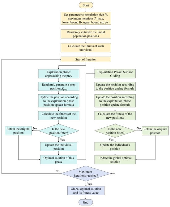
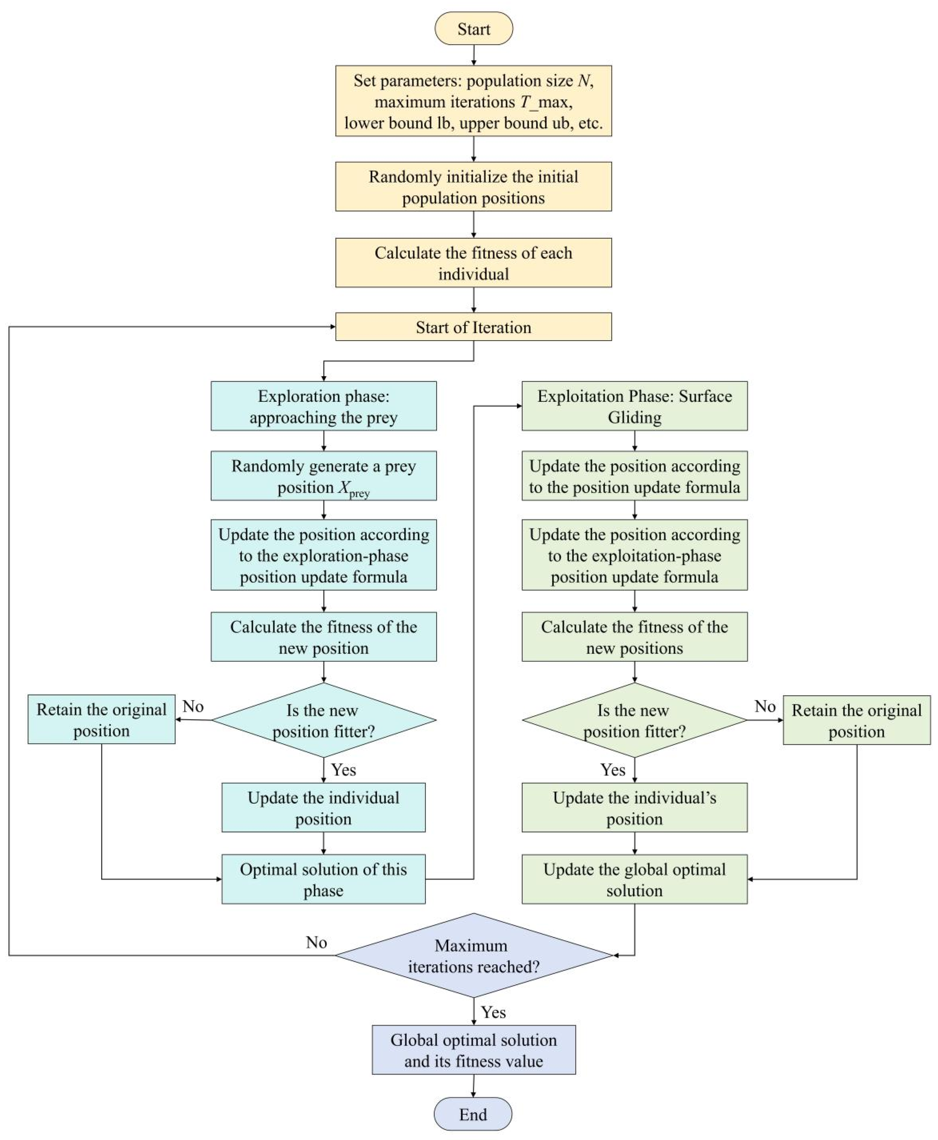
The POA is a nature-inspired swarm intelligence optimization algorithm that emulates the strategic hunting behavior of pelicans on the water surface. The algorithm searches the solution space efficiently by simulating the complete hunting process of pelicans, from spotting prey at a high altitude to precisely capturing it near the water surface. As shown in Figure 3, the algorithm consists of three stages: population initialization, global exploration, and local exploitation.
Figure 3.
Flowchart of the POA.
The first stage of the algorithm is population initialization. Let the dimension of the optimization problem be m, and let the population consist of N individuals. The position of the i-th individual (i.e., a candidate solution) can be expressed as follows:
Within the search space, the initial positions of the population are generated by uniform random sampling:
where lbj and ubj denote the lower and upper bounds of the j-th variable, respectively, and rand is a random number that is uniformly distributed over the interval [0, 1].
Once the population has been initialized, the algorithm enters the global exploration stage, which simulates pelicans spotting prey from the air and flying toward the prey area. In the algorithm, the position of the best individual in the current population is taken as the prey position. Each individual then updates its position according to the result of the fitness comparison with the prey:
In Equation (12), denotes the position of the i-th individual on the j-th dimension after the first-stage update; pj denotes the component of the prey position, Xprey, in the j-th dimension; F(·) denotes the fitness function; and I is a random integer that takes a value of either 1 or 2. When I = 2, the search step size is effectively enlarged, thereby strengthening the exploration ability of the algorithm. The updated position is retained according to the greedy criterion:
The final stage is local exploitation, which simulates pelicans using their wings to carry out fine predation on the water surface. In this stage, a small-range, high-precision search is conducted in the vicinity of each individual’s current position so that the population gradually approaches the optimal solution. The formula for an individual position update is as follows:
In Equation (14), denotes the position that is updated in the second stage; R denotes the local search radius constant, which is usually set to 0.2; t and Tmax denote the current and maximum iteration number, respectively; denotes a linearly decreasing time-decay factor that makes the search range contract gradually; and (2 ⋅ rand − 1) generates a random direction within the range [−1, 1]. After the update, the greedy selection mechanism is also used to retain the better position:
Through the alternating iteration of the exploration and exploitation stages described above, the standard POA gradually guides the population to converge toward the optimal solution. However, when applied to the high-dimensional, strongly nonlinear problem of path planning in karst areas, its linearly decreasing attenuation factor and fixed search strategy tend to produce an imbalance between convergence speed and solution accuracy. To address these issues, this study develops the IPOA by introducing two improvement mechanisms, namely, Lévy flight disturbance and a nonlinear convergence factor, which enhance the algorithm in terms of the diversity of search strategies and the adaptability of the convergence process, respectively [32].
2.4. A Multi-Strategy Improved POA
2.4.1. The Proposed Nonlinear Convergence Factor
In the local exploitation stage, the standard POA adopts a linearly decreasing convergence factor, which leads to a rigid convergence pattern, an imbalance between exploration and exploitation, and a lack of adaptive adjustment. On cultivated land in the karst areas of Guangxi, where fields are fragmented and field boundaries are highly irregular, the topology of the solution space is complex, and the shortcomings described above are further amplified. To overcome them, this study introduces an exponential nonlinear convergence factor to replace the original linear attenuation factor. Its mathematical expression is as follows:
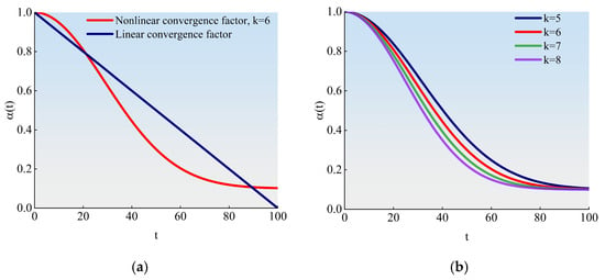
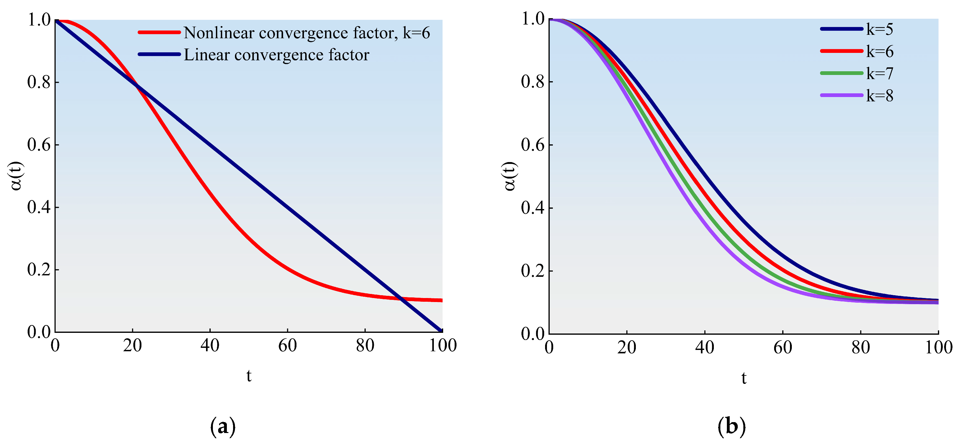
In Equation (16), t denotes the current iteration number; Tmax denotes the maximum iteration number; αmax denotes the initial convergence factor, set to 1.0 here; αmin denotes the final convergence factor, set to 0.1 here; and k denotes the attenuation intensity coefficient, which is chosen in the range [5, 8] and increased appropriately as the complexity of the field boundary shape increases. The exponential decay mechanism enables the convergence factor to decrease more rapidly during the early iterations (approximately the first 20), which quickly reduces the search step to locate high-quality solution regions, and then to decay more gradually in the middle and later stages, retaining an adequate step size for fine local convergence, making it better suited to the fragmented fields and irregular boundaries that are characteristic of the karst areas of Guangxi. After the nonlinear convergence factor is introduced, Equation (14) is modified as follows:
To balance the convergence speed of the algorithm against the quality of the final solution, the maximum number of iterations is set to 100. Figure 4a compares the attenuation curves of the standard linear convergence factor and the improved exponential nonlinear convergence factor (with the attenuation intensity coefficient k = 6) over the same number of iterations [33]. As can be seen from the figure, the nonlinear convergence factor decreases more rapidly during the early iterations (approximately the first 20), which helps the algorithm quickly locate the region of high-quality solutions; thereafter, the attenuation becomes more gradual, retaining a sufficiently large step size for fine local searching in the middle and late stages and thereby maintaining adequate diversity while the population approaches the optimal solution. Figure 4b presents the convergence curves for different values of k, demonstrating the regulatory effect of the attenuation intensity coefficient on the convergence pattern and providing a basis for flexibly setting the parameter according to the complexity of individual fields.
Figure 4.
Convergence curves of the nonlinear convergence factor. (a) The attenuation curves of the standard linear convergence factor and the nonlinear convergence factor (k = 6) at the same number of iterations. (b) Convergence curves of different k values.
2.4.2. Incorporating Lévy Flight Disturbance into POA
Lévy flight is a long-step random walk strategy that follows a Lévy distribution. Its step sizes take small values with high probability to support fine local searching while occasionally taking large values with low probability to produce substantial jumps, thereby establishing an effective balance between local exploitation and global exploration. Owing to this alternation between long and short steps, Lévy flight effectively prevents the algorithm from being trapped in local optima. In practice, the Mantegna algorithm is commonly used to approximate Lévy step sizes:
Here, β denotes a distribution parameter, usually set to 1.5, that controls the intensity of jumps; and are two independent random variables following normal distributions; and σv = 1; σu is calculated by the following formula:
where denotes the Gamma function.
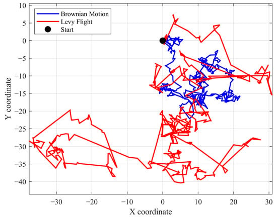
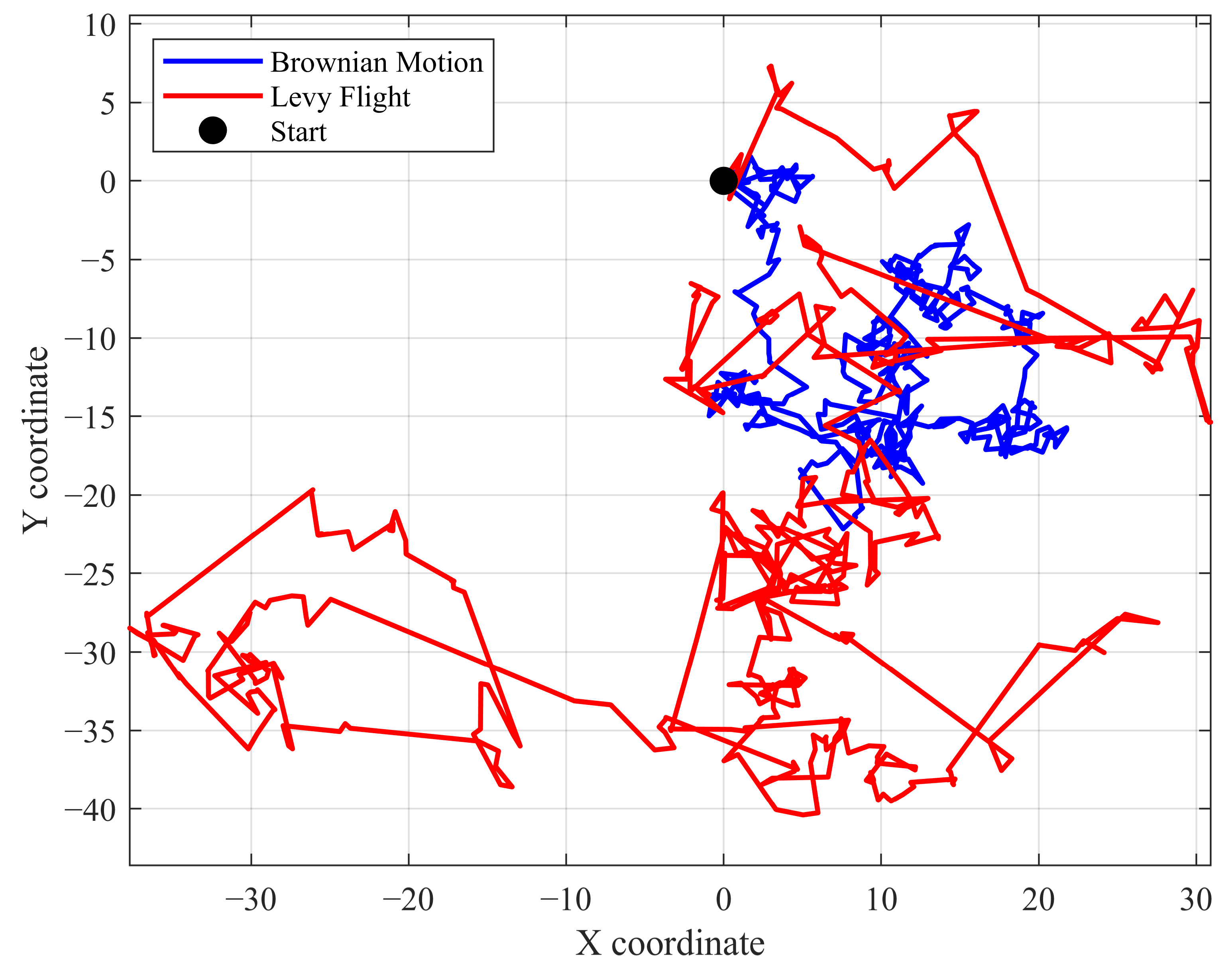
To provide an intuitive comparison between Lévy flight and conventional random search strategies [34], Figure 5 presents the trajectories of Lévy flight and standard Brownian motion over the same number of iterations (500). As can be seen from the figure, long-step jumps occur frequently in the Lévy flight trajectory, giving it a much wider exploration range than Brownian motion, which always moves in uniform steps. This characteristic endows Lévy flight with a stronger global search capability [35].
Figure 5.
Trajectory comparison between Lévy flight and Brownian motion.
Based on these characteristics, this study introduces the Lévy perturbation mechanism into both the global exploration and local exploitation stages of the standard POA. Specifically, in the global exploration stage, after the individual positions have been updated, Lévy jump perturbation is applied to selected individuals; while the population as a whole continues to converge toward the optimal region, these individuals retain a probability of moving far away from the current aggregation area to conduct large-scale searches, thereby broadening the scope of global exploration. In the local exploitation stage, a small Lévy perturbation is applied to the current optimal solution to promote fine searching in its neighborhood and increase the probability of finding a better solution. By adaptively adjusting the perturbation step size, this mechanism optimizes the dynamic balance between coverage of the entire space and exploitation of local regions.
2.4.3. The Design of the Improved Strategies
The two improvement strategies described above enhance the performance of the standard POA in different ways. The Lévy flight disturbance acts primarily at the search strategy level: it increases population diversity through a random walk that alternates between long and short steps and helps the algorithm escape from local optima, and its influence extends throughout the entire iteration process. The nonlinear convergence factor acts primarily at the level of convergence process control: it regulates the rhythm of exploration and exploitation through exponential decay, ensuring that the algorithm maintains extensive exploration in the early iterations and concentrates on fine exploitation in the later stage.
The two mechanisms work in a coordinated manner: the Lévy flight disturbance provides sufficient population diversity to ensure that the nonlinear convergence factor can function during global search, while the nonlinear convergence factor, through a reasonable decay rhythm, allows the high-quality solutions generated by the Lévy flight disturbance to be fully exploited. Together, the two improvement mechanisms enhance the adaptability and robustness of the algorithm when handling practical constraints such as fragmented cultivated land and complex boundaries in the karst areas of Guangxi. The pseudo-code of the IPOA is shown at here (Algorithm 1):
| Algorithm 1. Improved Pelican Optimization Algorithm (IPOA) | |
| Require: population size N, max iterations Tmax, dimension D, unit coding interval [0,1], fitness f, Levy exponent β = 1.5, Levy probability plevy = 0.5 (global exploration); 0.2((local exploitation), Levy coefficients αL = 2.0, βlevy = 1.5, nonlinear factors αmax = 1.0, αmin = 0.1, k ∈ [5,8], local radius R = 0.2. Ensure: optimal solution xbest and its fitness. | |
| 1: | // Initialization (before the generational loop; not counted in the 10,000-FE budget) |
| 2: | xi = rand(D) ∈ [0,1]D, i = 1,…,N |
| 3: | evaluate fi = f (xi); identify prey xprey (best solution) |
| 4: | FE←0 generational evaluation counter |
| 5: | while FE<10,000 do |
| 6: | Global exploration phase N objective calls |
| 7: | for i =1 N do |
| 8: | I = rand i ([1,2]) |
| 9: | if f (xprey) < fi then |
| 10: | xnew = xi + rand•(xprey – I•xi) |
| 11: | else |
| 12: | xnew = xi + rand•(xi – I•xprey) |
| 13: | end if |
| 14: | if rand < plevy then |
| 15: | xnew← xnew +αL·L(β) position-only; no extra f-call |
| 16: | end if |
| 17: | clip xnew to [0, 1]; evaluate fnew = f (xnew); FE←FE+1 |
| 18: | if fnew<fi then xi = xnew, fi = fnew |
| 19: | end if |
| 20: | end for |
| 21: | update xprey from current population |
| 22: | Local exploration phase N objective calls |
| 23: | compute |
| 24: | for i =1 N do |
| 25: | xnew=xi+ R · α(t) · (2rand-1) · xi |
| 26: | clip to [0,1] and evaluate fnew = f (xnew); FE←FE+1 |
| 27: | update xi if improved |
| 28: | end for |
| 29: | xprey ← clip[0,1] (xprey +βlevy · Lbest(β)) position-only; evaluated in the next regular phase, no extra f-call |
| 30: | end while |
| 31: | return xprey, f (xprey) |
Regarding the representation of solutions, because the traversal order of the operation rows constitutes a discrete permutation problem, whereas IPOA updates positions in a continuous space, a sorting-based mapping is required to decode continuous vectors into discrete permutations. In this study, the ranked-order value (ROV) rule is adopted: the components of each individual position vector are sorted in ascending order of their numerical values, and the rank assigned to each component determines the corresponding order in which the operation rows are visited. For example, the ROV rule maps a position vector to a non-repeating permutation of the integers from 1 to d. After the algorithm completes its position update in the continuous space, this mapping is decoded into a feasible operation row sequence for fitness evaluation.
In terms of constraint handling, the permutation constraint is inherently satisfied through the ROV mapping, which yields non-repeating permutations of the integers from 1 to d. Consequently, each operation row is visited exactly once, with neither repeated visits nor omissions. The turning-envelope constraint is satisfied by the 6.0 m contraction width of the external spiral operating area: because this width exceeds the outermost trajectory radius corresponding to the minimum turning radius, all turns are completed without violating the minimum turning radius constraint. The boundary constraint is enforced by restricting each component to its search interval during position updates, with any component that crosses a boundary being truncated at the boundary value. On this basis, the feasibility of every candidate solution is verified from three aspects: coverage rate, compliance with the minimum turning radius, and boundary crossing. All planned paths are thereby confirmed to be feasible. For concave boundary sections, the swept envelope of the machine, rather than only its centerline, is checked against the field polygon: the outermost swept trajectory is tested for intersection with every boundary segment, and a candidate is rejected if any part of the envelope crosses the boundary or enters a concave indentation, so a feasible centerline alone is not accepted.
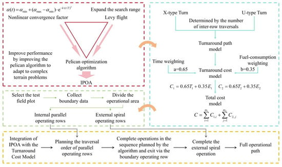
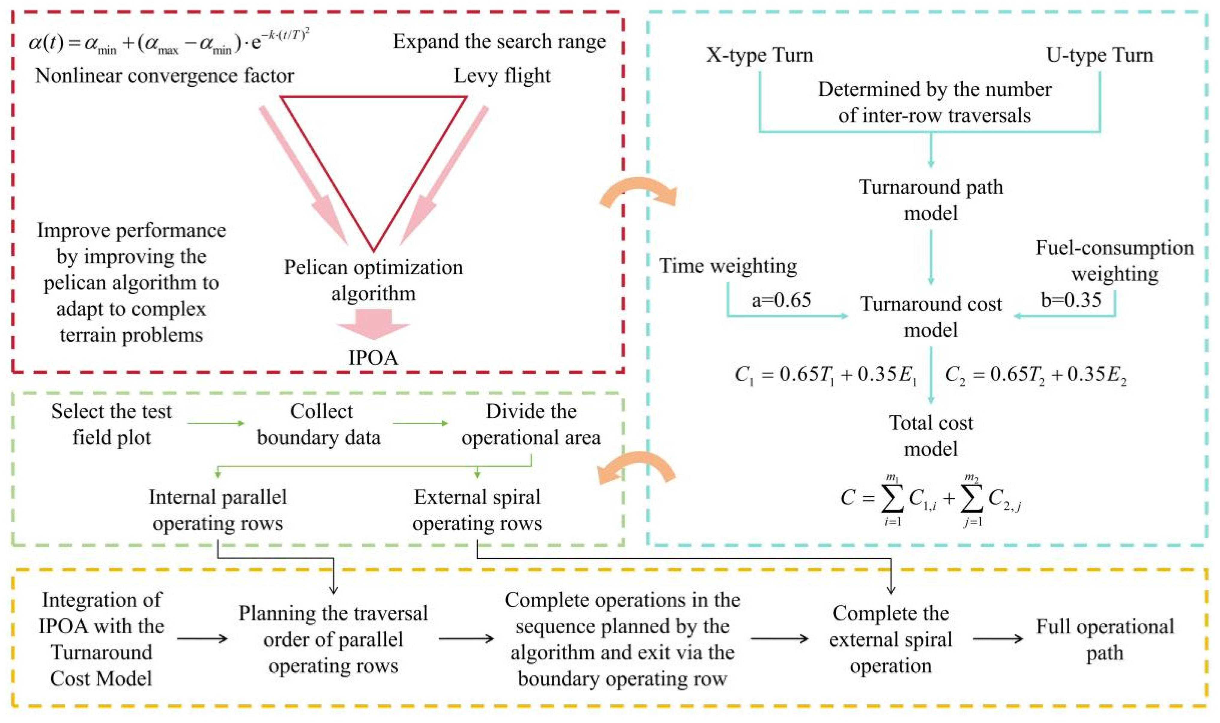
The IPOA is then combined with the adaptive turning model, and the total turning cost incurred in completing an operation is taken as the fitness function to globally optimize the traversal order of the internal parallel operating rows. The overall technical flowchart of the proposed method is presented in Figure 6.
Figure 6.
Overall technical flowchart. The red dashed box summarizes the improved IPOA, the blue dashed box the turning-cost model, the green dashed box the field-data processing, and the yellow dashed box the integration and output; the arrows indicate the workflow direction.
3. Case Analysis
3.1. Data Acquisition and Simulation Experiments
3.1.1. Field Boundary Data Acquisition
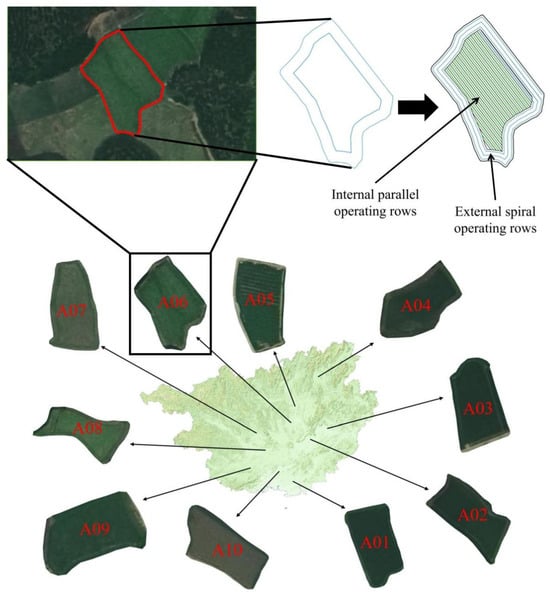
To verify the effectiveness of the turning cost model and the IPOA developed in this study and to conduct the simulation experiments, ten paddy fields exhibiting the typical characteristics of karst cultivated land in Guangxi were selected as test objects, and the ArcGIS Pro 2024 (Esri, Redlands, CA, USA) platform was used for the digital acquisition of their boundaries [36]. The distribution of the fields and the subsequent data processing workflow are shown in Figure 7.
Figure 7.
Acquisition and preprocessing of field boundary data. A01–A10 denote the ten test fields; the red outline denotes the digitized field boundary, the blue outlines the extracted vector polygon, and the green lines the divided operation rows.
First, the closed boundary of each field was manually identified and outlined from high-resolution remote sensing images to obtain vector polygon data. The perimeter, P, and area, A, of each field were then extracted using the measurement tools in ArcGIS. To further quantify the complexity of the field boundaries, the area–perimeter ratio (APR) was introduced as an evaluation metric, defined as follows:
This ratio reflects the compactness of the field shape. Under the same area, fields with more tortuous boundaries and more irregular shapes have larger perimeters and consequently smaller APR values. In other words, a smaller APR indicates a more complex field boundary and higher spatial heterogeneity, whereas a larger APR indicates a shape that is closer to a regular form. The relevant geometric parameters of the ten test fields are listed in Table 1.
Table 1.
Geometric information of the test fields.
As shown in Table 1, the areas of the ten test fields range from 1825.49 to 2976.52 m2, their perimeters from 186.23 to 241.62 m, and their APR values from 8.32 to 13.02. The fields include a variety of boundary forms, from relatively regular to highly irregular, and can therefore adequately represent the geometric diversity of cultivated land in the karst areas of Guangxi.
3.1.2. Working Area Division
Once the field boundary has been obtained, it must be converted into a sequence of operating rows that can be processed by the algorithm. To reduce the spatial constraints on the turning maneuvers of the agricultural machinery and improve the uniformity and completeness of sowing coverage, each field was divided into two functional areas: the internal parallel operating area and the external spiral operating area [37].
The internal parallel operating area is the principal area in which the agricultural machinery performs seeding and consists of a set of equally spaced parallel operating rows. The external spiral operating area is the annular zone between the parallel operating area and field boundary; its main function is to provide the buffer space required for turning maneuvers after the machine completes a single row in the parallel operating area. The boundary between the two areas was determined by a boundary contraction operation: the original field boundary was contracted inward equidistantly by a certain width, and the enclosed region after contraction formed the internal parallel operating area, whereas the annular zone between the original and contracted boundaries formed the external spiral operating area. The width of this zone must satisfy the minimum space required for the machine to complete a turning maneuver in one pass. Given that the minimum turning radius of the machine is 3.1 m and the overall machine width is 1.9 m, the radius of the outermost trajectory during turning is 3.1 + 1.9 = 5.0 m. Therefore, to ensure smooth turning maneuvers, the external spiral operating area was set to contain the width of three operating rows, giving a total contraction width of 6.0 m, which fully covers the outermost trajectory radius required for turning.
The division of operating rows within the parallel operating area follows the principles outlined below. First, to minimize the total number of operating rows and reduce the frequency of turning maneuvers, the longest side of the field was selected as the reference edge, and the operating rows were oriented parallel to this edge. Second, starting from the side on which the reference edge lies, operating rows were divided inward at an equal spacing of 2.0 m and numbered sequentially. This number sequence constitutes the basic element to be optimized by the subsequent path planning algorithm, as the optimal traversal order output by the algorithm is a permutation of these numbers. Because the actual seeding width of the machine is 1.9 m, whereas the center-to-center row spacing is set to 2.0 m, each working pass leaves an unsown strip of about 0.1 m. This spacing is deliberately adopted to provide sufficient clearance for the machine to travel between passes, so the unsown strip is limited to 0.1 m per pass and the resulting coverage rate is approximately 95% (1.9 m/2.0 m), which remains above 90%. The 2.0 m spacing is therefore retained for the geometric layout and the turning-cost calculation.
The external spiral operating area is not an object of algorithmic optimization but rather a spatial guarantee for the turning maneuvers of the machine. After the machine completes the last operating row in the parallel operating area, it transfers to the nearby external spiral operating area and completes the sowing of the remaining area along a spiral path. The path of this section is generated according to a fixed spiral rule and is not part of the traversal order optimization.
3.1.3. Simulation Experiments
After the acquisition of field boundary data and division of the working area were completed, simulation experiments were conducted on the MATLAB R2024b (MathWorks, Natick, MA, USA) platform. The composite index C was used as the core evaluation metric, while the operation path length S, operation time T, and fuel consumption E were used as auxiliary indices, enabling the planning performance of each algorithm to be comprehensively evaluated from multiple perspectives.
For each test field, the boundary vector data were first imported, and the working area division described in Section 3.1.2 was performed to generate the number sequence of the internal parallel operating rows. The turning cost model was then embedded in the IPOA to optimize the access order of the operating rows, with the objective of minimizing the composite index C; after this, the optimal traversal order and its corresponding cost indices were output. The IPOA was subsequently replaced by the standard POA, as well as the GA, ACO, and PSO, which were used to plan paths for the same batch of test fields under identical conditions, providing a comparison with the IPOA results. The comparison was organized into two levels. The first level compared the IPOA with the classical POA to verify the effectiveness of the two improvement strategies introduced in this study, namely, Lévy flight disturbance and the nonlinear convergence factor. The second level compared the IPOA with the GA, ACO, and PSO—three algorithms that are commonly used in path planning—to comprehensively evaluate the performance advantages of the IPOA relative to mainstream algorithms.
Because intelligent optimization algorithms are stochastic, the result of a single run may be subject to statistical fluctuation. To eliminate the influence of accidental factors on the conclusions, each algorithm was run independently 30 times on the same field, with different random seeds and the same population size of N = 50 being used in every run. To ensure a fair comparison, all algorithms were evaluated under a unified budget of function evaluations (FEs). Because each generation of the POA and IPOA comprises two search stages, it consumes 2N evaluations per generation, whereas the GA, ACO, and PSO consume N evaluations per generation. The termination condition for every algorithm was that the cumulative number of generational FEs reached the prescribed budget, which was set to 10,000 in this experiment; this budget counts only objective calls made inside the iterative loop, while the N evaluations used to initialize the population are performed before the loop and are not counted. The Lévy perturbations modify candidate positions only and trigger no additional objective calls, so each IPOA/POA generation still contributes exactly 2N evaluations. The mean, standard deviation, best, and worst values of each metric were recorded over the 30 runs. Pairwise comparisons were conducted using the Wilcoxon rank-sum test at a significance level of α = 0.05, and the Friedman test together with the Nemenyi post hoc test was used to compare multiple algorithms. The experiments are analyzed systematically, focusing on five aspects: path length, operation time, fuel consumption, composite index C, and convergence performance. The principal parameter settings of IPOA are consolidated in Table 2; the same settings were used for every field and every independent run.
Table 2.
The principal parameter settings of IPOA.
3.2. Effectiveness Verification of the Improvement Strategies
After the simulations, the mean and standard deviation of each metric over the 30 runs of the IPOA and POA were calculated and are presented in Table 3. As shown in the table, the mean values of S, T, E, and C obtained by the IPOA are lower than those obtained by the POA on all ten test fields, which verifies the effectiveness of the improvement strategies proposed in this study. Here S, T, E, and C are reported for the complete field operation of each traversal sequence, i.e., the parallel working passes inside the field together with the headland turns that connect them, rather than for the turning maneuvers alone. The straight working-pass length is fixed by the field geometry, while the turning contribution is the component that varies with the traversal sequence.
Table 3.
Comparison of the mean and standard deviation results of IPOA and POA.
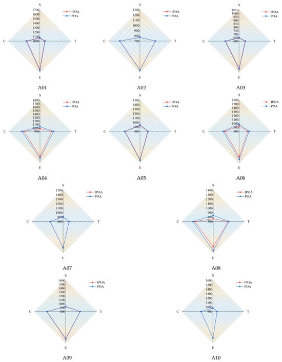
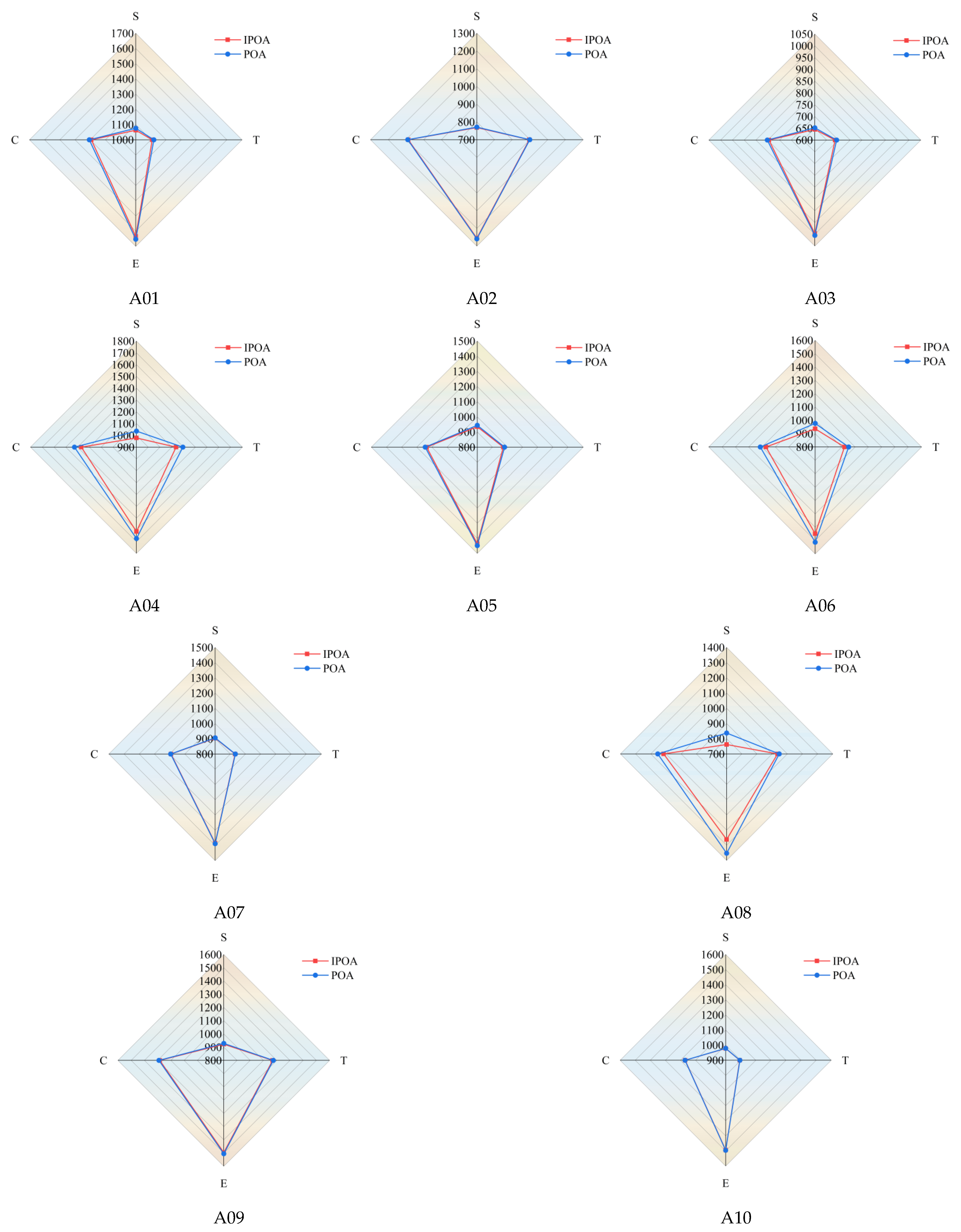
Figure 8 presents the comprehensive performance of the two algorithms across the different metrics in the form of radar charts. For a given field, the area that is enclosed by the polygon connecting the metrics provides an overall measure of the algorithm’s optimization performance. As shown in the figure, the IPOA encloses a smaller radar area on all ten test fields, indicating that its average performance is consistently superior. The difference between the two algorithms is most pronounced on field A04, where the mean path length decreases from 1035.98 m for the POA to 978.07 m for the IPOA, a reduction of 5.59%; the operation time, fuel consumption, and composite index C are reduced by 4.43%, 3.55%, and 4.07%, respectively. The metrics for the remaining fields also improve to varying degrees. These results demonstrate that the Lévy flight disturbance and nonlinear convergence factor introduced in this study effectively enhance both the global exploration capability and the local exploitation accuracy of the algorithm, thereby yielding better path planning schemes.
Figure 8.
Comparison of the mean results of IPOA and POA. Each subfigure corresponds to one test field (A01–A10); the red curve with square markers represents the IPOA, the blue curve with circular markers represents the POA, and the four axes denote path length (S), operation time (T), fuel consumption (E), and composite index (C).
A further comparison of the reductions across fields reveals that the magnitude of improvement does not exhibit a significant monotonic relationship with the APR, which reflects shape compactness. The Spearman correlation coefficient between the APR and the composite index C reduction across the ten fields is only −0.03, indicating that the APR alone cannot predict the magnitude of the algorithm’s improvement. Indeed, the three fields with the largest composite index C reductions are A04, A06, and A08, where costs are reduced by 4.07%, 3.51%, and 3.34% and whose APR values are 10.97, 11.96, and 8.32, respectively; these values are not concentrated in the lowest APR range. This indicates that the room for improvement in path planning depends not only on the compactness of the field shape but also on the number of rows and their geometric distribution, as well as on the switching between X- and U-type turns that is induced by local concave and convex boundary features. From the perspective of the algorithmic mechanism, because the POA employs a single search method and its exploration directions are limited, it is prone to premature convergence on fields containing numerous local optima. In contrast, the IPOA enhances its ability to escape local optima through the long-range jumps provided by Lévy flight, and its improvement is more evident on fields where the POA is prone to stagnation, demonstrating stronger adaptability and robustness.
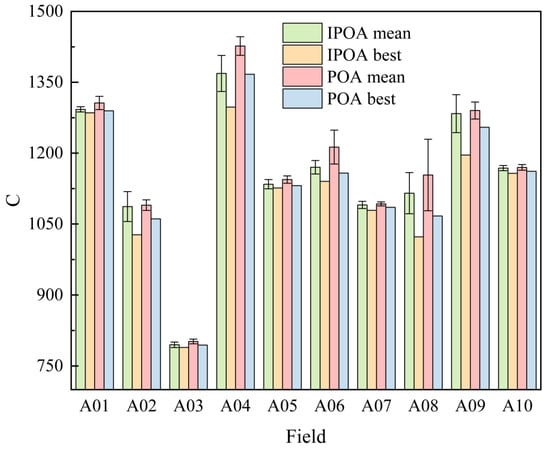
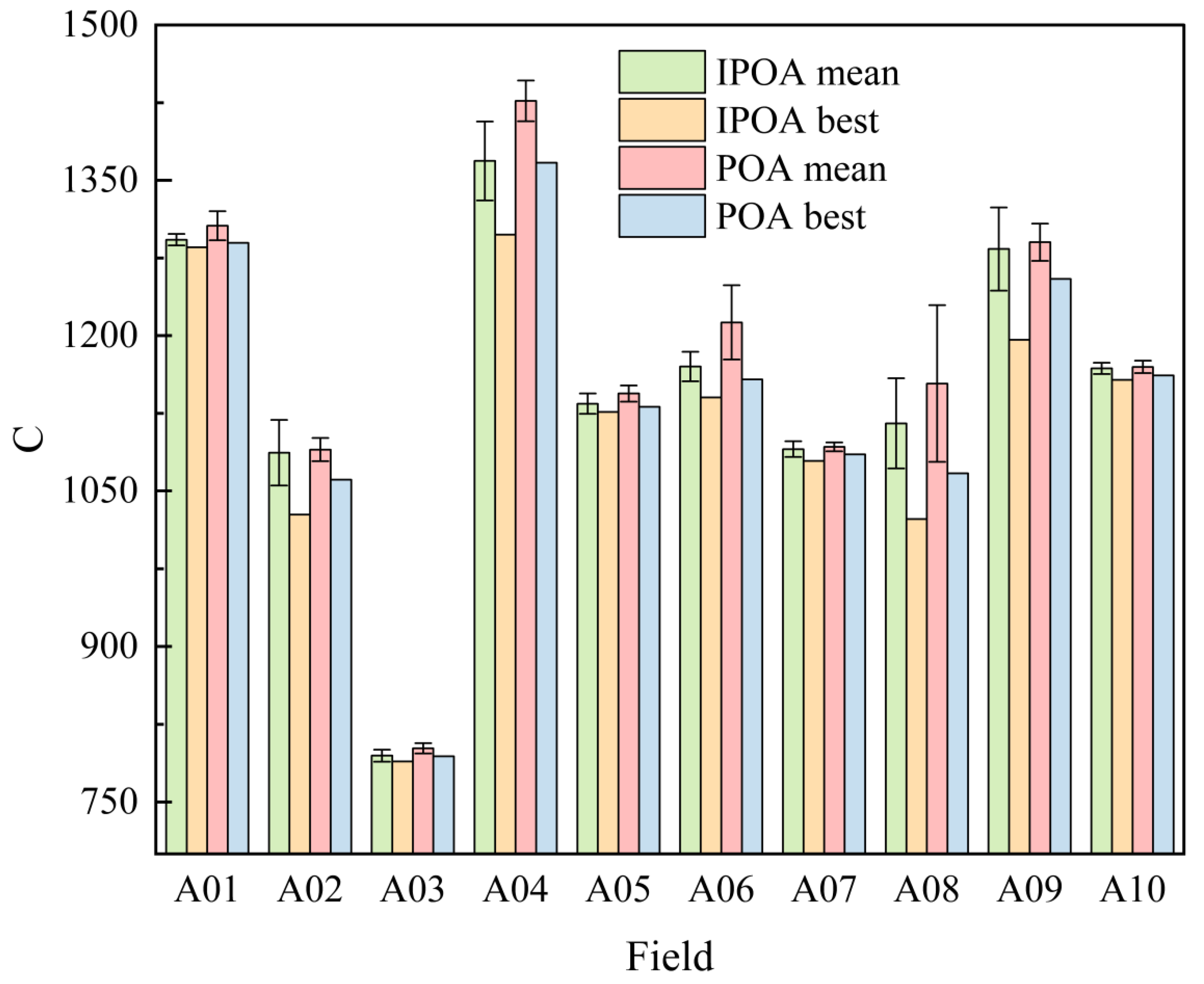
Figure 9 compares the mean and best values of the composite index C obtained by the IPOA and POA on the ten fields; this is presented using a grouped histogram, in which the error bars attached to the mean columns represent the standard deviation. As shown in the figure, both the mean and best values of the IPOA are lower than the corresponding values of the POA on every field, further confirming the advantage of the improvement strategies in terms of solution quality. More importantly, the relationship between the mean and best values differs markedly between the two algorithms. On most fields, the best value column of the IPOA is close to the height of its mean column, indicating that it can stably converge to a near-optimal level across the 30 runs and that the results exhibit good repeatability. The gap between the best and mean values of the POA is larger, particularly for fields such as A06 and A08, which shows that although the POA can occasionally find a better solution, most of its runs deviate from that best value and that its stability is insufficient. In line with this, the error bars of the IPOA are shorter on fields such as A06 and A08, where the POA fluctuates substantially. Even though the error bars of the IPOA are larger than those of the POA on a few fields, the IPOA remains superior owing to its smaller mean value and better best value. These results show that the IPOA not only achieves a lower composite index C but also delivers better consistency and reliability over multiple independent runs, which is of practical importance for agricultural machinery operations that depend on stable planning results.
Figure 9.
Comparison of optimal and mean values of C between IPOA and POA.
3.3. Comparative Evaluation of Different Algorithms
To further evaluate the comprehensive performance of the IPOA, the results of 30 runs of the GA, ACO, and PSO were also compiled, and the mean and standard deviation of each metric are presented in Table 4. As shown in the table, the mean composite index C of the IPOA is the lowest on all ten test fields, giving it a clear advantage over the other algorithms.
Table 4.
Comparison of the mean and standard deviation results of IPOA and other algorithms.
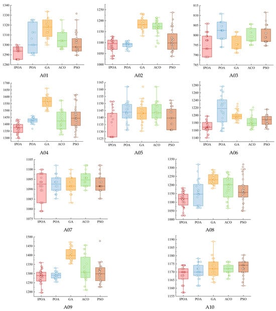
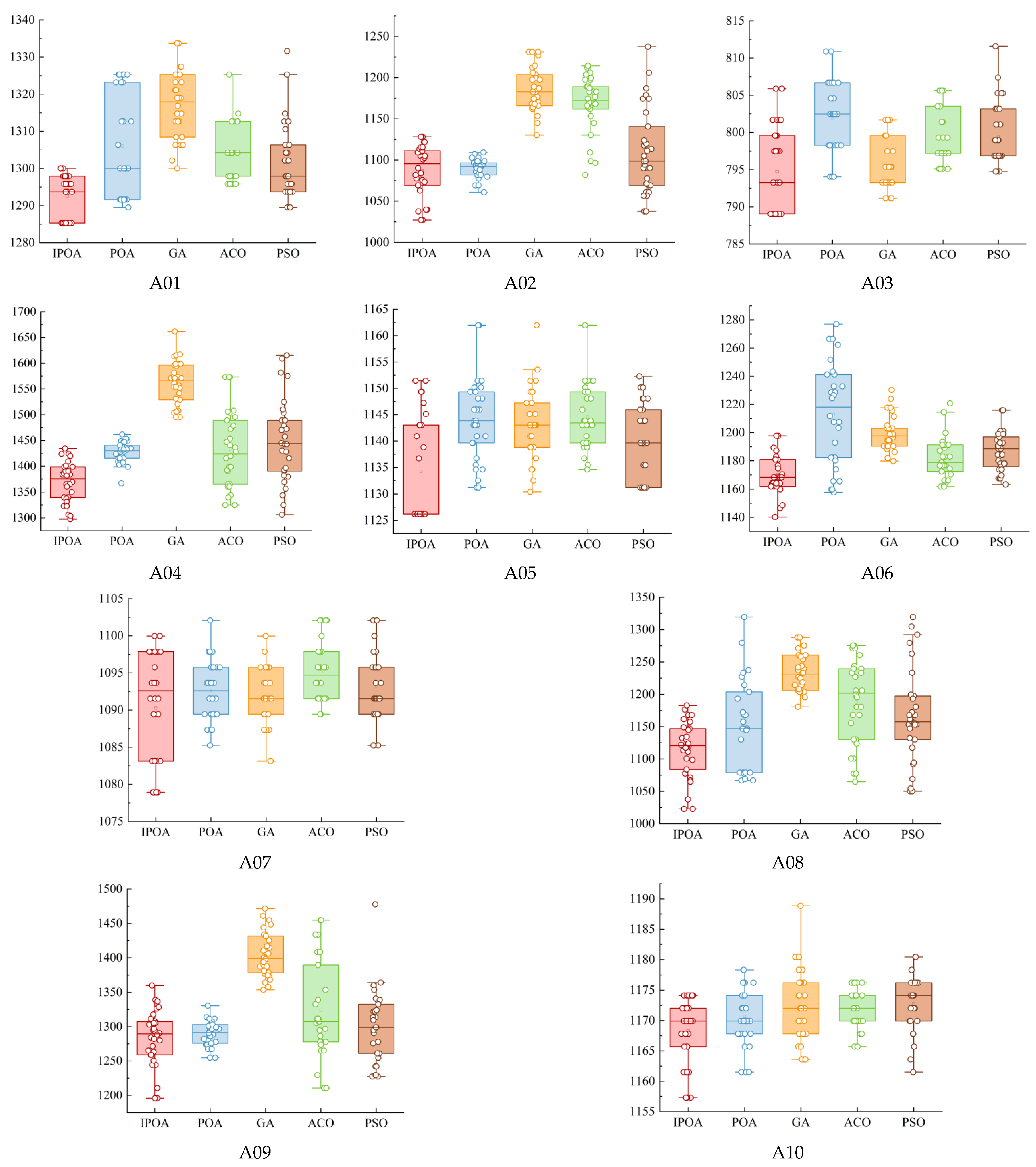
Figure 10 presents the distribution of the composite index C obtained by the five algorithms over 30 runs based on the ten fields in the form of box plots, in which the position of each box reflects the median and quartile levels and the individual points represent the scatter points and outliers. As shown in the figure, the box of the IPOA is located at the lowest position on most fields and is relatively compact, indicating a lower median and a more concentrated distribution. The boxes of the GA and PSO are generally positioned higher, and several fields exhibit more outliers and a wider dispersion. To quantify the performance gap, the mean difference in composite index C between each algorithm and the IPOA was further calculated. The IPOA achieves the largest mean reduction relative to the GA, with an average reduction of approximately 4.46% across the ten fields, followed by the ACO at approximately 2.44%; the corresponding mean reductions relative to the PSO and POA are approximately 1.72% and 1.48%, respectively. For specific fields, the composite index C of the IPOA on field A09 is 3.03%, 8.58%, and 1.31% lower than that of the ACO, GA, and PSO, respectively, whereas the corresponding reductions on field A05 are 0.90%, 0.73%, and 0.43%. The magnitude of improvement differs considerably across fields. Consistent with the findings above, this difference is governed mainly by the degree of premature convergence of each algorithm under the specific field geometry. Because its linear progressive search is inefficient under complex constraints, the GA exhibits the largest gap from the IPOA. Although the ACO is close to the IPOA on some fields, the gap widens on A02 and A08, and its stability is insufficient. The PSO is prone to premature stagnation and shows large overall fluctuations. The comparison further confirms that the IPOA possesses superior and more stable optimization capability in comparison with multiple algorithms.
Figure 10.
Boxplot of the planning results of each algorithm. Each subfigure corresponds to one test field (A01–A10); the five boxplots show the distribution of the composite index C over 30 independent runs for the IPOA (red), POA (blue), GA (orange), ACO (green), and PSO (brown), with the box indicating the interquartile range, the horizontal line the median, and the dots the individual runs and outliers.
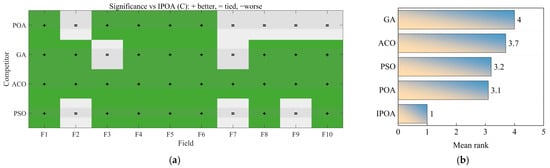
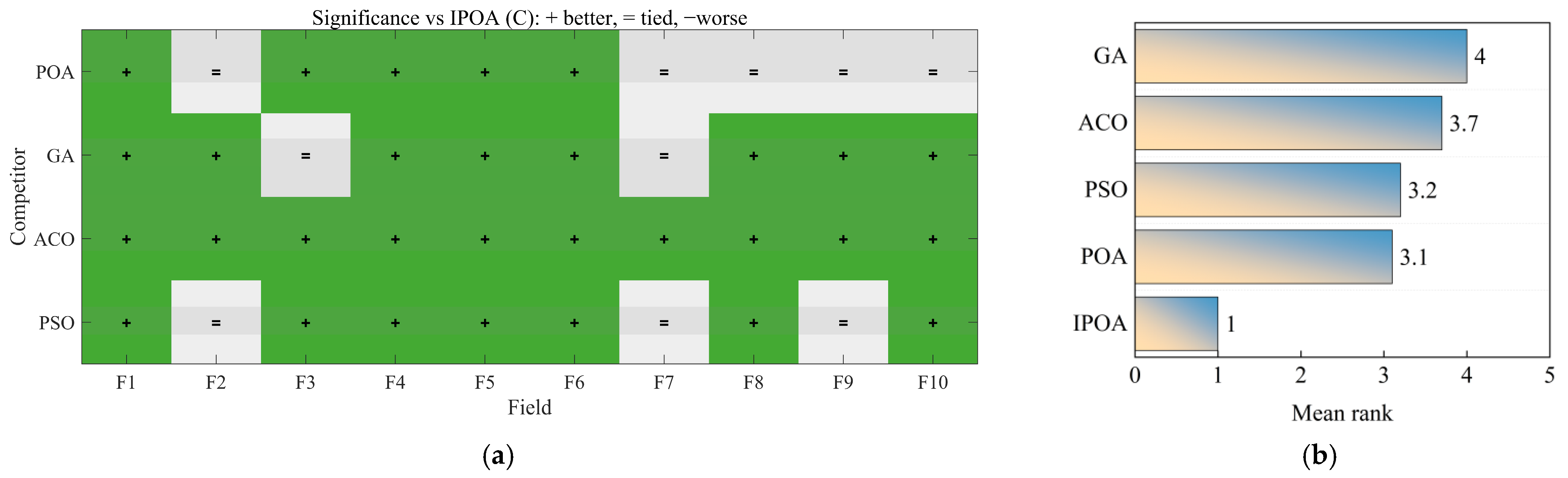
Statistical tests were conducted on the planning results of the five algorithms across the ten fields at a significance level of α = 0.05. The Wilcoxon rank-sum test was used to compare the IPOA with each of the other four algorithms. The results are shown in the heat map in Figure 11a, where a green ‘+’ indicates that the IPOA is significantly better than the corresponding algorithm and a gray ‘=‘ indicates that the difference is not significant. Judging from the number of fields on which the differences are significant, the IPOA is significantly superior to the ACO on all ten fields, as well as to the GA, PSO, and POA on most fields, and there is no case in which the IPOA is significantly worse. Furthermore, the Friedman test was used to compare the algorithms as a whole, and a critical difference in CD = 1.93 was obtained through the Nemenyi post hoc test. The mean ranks of each algorithm are shown in Figure 11b. The IPOA has the lowest mean rank, followed by the POA, PSO, ACO, and GA. The differences in mean rank between the IPOA and the POA, PSO, ACO, and GA are 2.1, 2.2, 2.7, and 3.0, respectively, all of which exceed the CD and are therefore significant. The rank differences among the four comparison algorithms are all smaller than the CD and hence not significant. This demonstrates that the overall performance of the IPOA is significantly better than that of the other algorithms, whereas the comparison algorithms cannot be significantly distinguished from one another.
Figure 11.
(a) IPOA’s winning and losing heat maps compared with other algorithms for each field. (b) Friedman average rank of each algorithm.
For full traceability, the Friedman test treats the ten fields as ten blocks (N = 10) and the five algorithms as the treatments. Within each block, the five algorithms are ranked on the composite index over the 30 independent runs, and the algorithm ranks are then averaged across the ten blocks to give the mean ranks in Figure 11b (IPOA 1.0, POA 3.1, PSO 3.2, ACO 3.7, GA 4.0). The Friedman statistic is χ2 = 22.160 with p = 0.0001862. The Nemenyi critical difference is computed from CD = q0.05 · sqrt(k(k + 1)/(6N)) with k = 5 algorithms, N = 10 blocks and the tabulated critical value q0.05 = 2.728, giving CD = 1.93; two algorithms differ significantly only when their mean-rank difference exceeds this value. The Nemenyi procedure already accounts for the family-wise multiple-comparison adjustment, whereas the pairwise Wilcoxon tests in Figure 11a are reported as unadjusted field-level comparisons at α = 0.05 and are interpreted together with the corrected omnibus ranking rather than as independent confirmations.
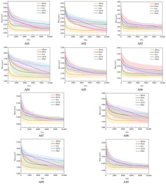
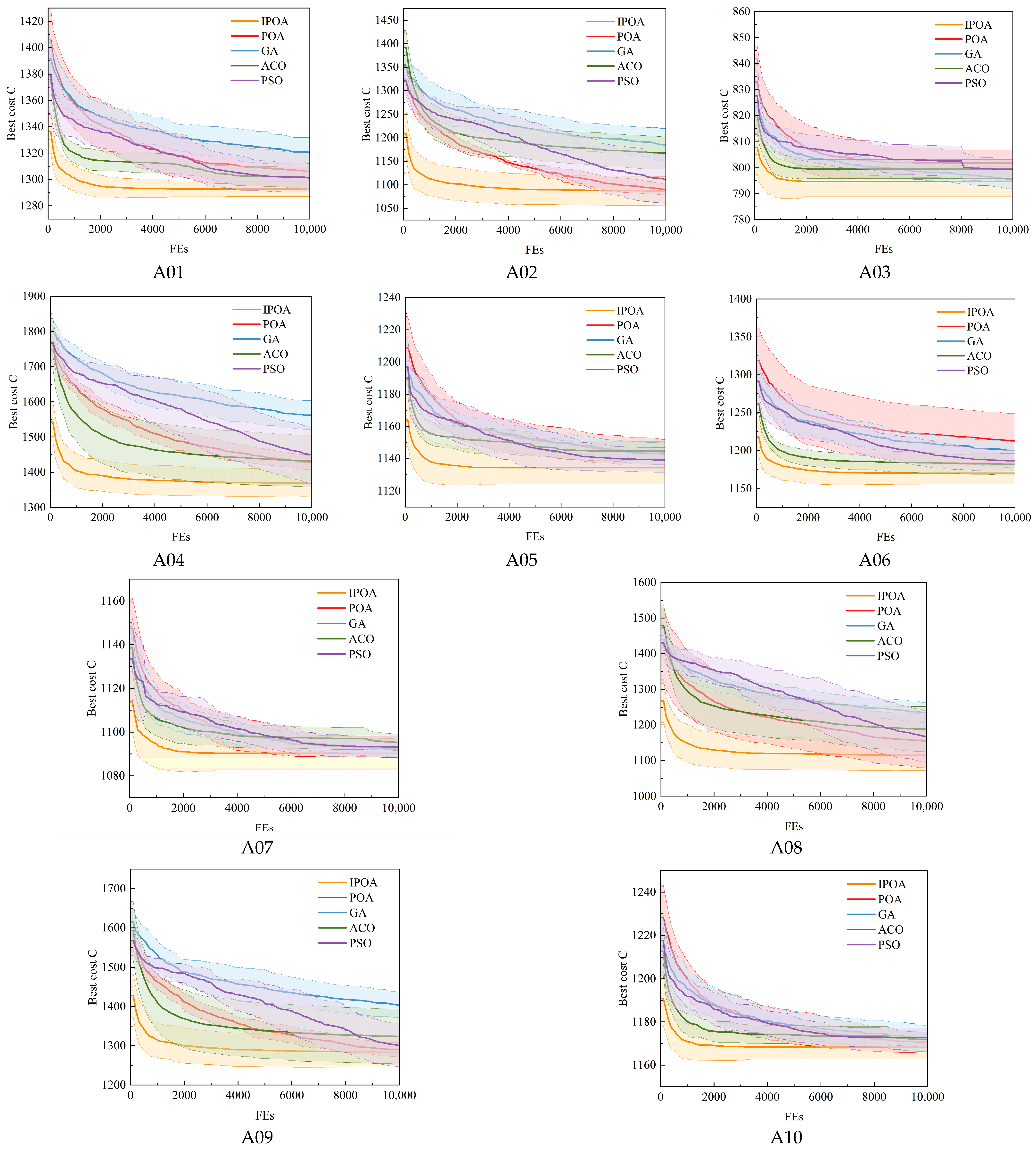
The iteration curves of each algorithm on each test field are shown in Figure 12, with the horizontal axis representing the cumulative number of function evaluations (FEs). In terms of convergence speed, the IPOA clearly outperforms the GA and PSO. On many fields with complex boundaries, the curves of the GA and PSO continue to decline throughout the FE budget, and on some fields, no obvious plateau appears before the FEs are exhausted, indicating that they have not yet converged to a stable optimal solution. Should additional evaluations be allowed, further improvement might still be possible, which reflects their low optimization efficiency and high consumption of computational resources. Although the final composite index C of the POA is close to that of the IPOA on many fields, its convergence is slower: on most fields, it requires more FEs to approach the final solution and therefore incurs a higher computational cost than the IPOA. The convergence performance of the ACO is insufficiently stable and exhibits a clear polarization. On fields such as A03 and A05, the ACO reaches a plateau after only a small number of FEs, and this premature convergence indicates that it has become trapped in local optima, resulting in a final composite index C that is much higher than that of the IPOA. On fields such as A02 and A07, however, the ACO converges too slowly and is still declining after more than half of the FEs have been consumed, which shows that its search direction lacks effectiveness in the complex constraint space and that it cannot locate the high-quality solution region rapidly during the early exploration stage.
Figure 12.
The iterative process curve of each algorithm. Each subfigure corresponds to one test field (A01–A10); the five curves show the convergence of the best composite index C with cumulative FEs for the IPOA (orange), POA (red), GA (blue), ACO (green), and PSO (purple), and the shaded bands indicate the standard deviation over 30 independent runs.
In terms of convergence accuracy, the IPOA attains the lowest composite index C on every field, and its curve shows a smooth convergence pattern characterized by a rapid initial decrease followed by gradual stabilization. When few FEs have been consumed, it declines rapidly and approaches the optimal solution region quickly. In the middle and later stages, the decline becomes more gradual while still retaining a certain capacity for improvement, and the curve enters a stable plateau after the cumulative FEs reach approximately one-third of the budget. This convergence characteristic stems from the introduction of the nonlinear convergence factor, which maintains a large search step during the early stage to explore the solution space thoroughly and then shrinks the search range to support fine local exploitation in the later stage, with a smooth and natural transition between the two. In contrast, although the PSO can continue to improve, its rate of decline remains low throughout the process and it is not fully converged on some fields when the FEs are exhausted, indicating low efficiency. The ACO either stagnates prematurely or lacks momentum in the later stage and provides no effective regulation of the search process; although the final accuracy of the GA is acceptable, its early convergence is too slow to establish a sound foundation for subsequent optimization.
Overall, although the final composite index C of the ACO is close to that of the IPOA on some fields, its convergence is clearly slower and more FEs and computational time are required to achieve comparable solution quality. In practical applications, this implies longer planning time and greater occupation of computational resources, and its comprehensive efficiency is therefore lower than that of the IPOA. The composite index C and convergence speed of the GA are both unsatisfactory, and its linear progressive search mechanism is inefficient in handling the highly nonlinear constraints of karst cultivated land. The performance stability of the PSO is the weakest, with substantial fluctuations across fields, making it difficult to use as a reliable tool for agricultural machinery path planning in karst areas. In contrast, the IPOA achieves a favorable balance among the three indicators of solution accuracy, convergence speed, and stability and exhibits the best or second best comprehensive performance in every comparison.
In summary, the IPOA outperforms the POA, GA, ACO, and PSO on the four core metrics of path length, operation time, fuel consumption, and composite index C, and the Wilcoxon and Nemenyi tests confirm that its overall performance in mean solution quality is significantly superior. This gain in the mean should be distinguished from a reduction in variability: the standard deviation of the IPOA is in fact larger than that of the POA on fields A02, A04, and A09, although it is smaller on the remaining fields, so improved repeatability is not uniform across fields. The IPOA has a moderate convergence speed and consistently returns high-quality, lower-cost planning schemes under a unified computational budget, making it more suitable for the engineering practice of agricultural machinery operation path planning in the karst areas of Guangxi. It should be noted that all the results described above are estimates from model simulations, that no significant monotonic relationship exists between the magnitude of improvement and the APR of a field, and that the practical engineering performance still requires further verification.
4. Conclusions
This study addresses three problems in the path planning of agricultural machinery in the karst areas of Guangxi: tortuous field boundaries, limited turning space, and the need to account for both operation time and fuel consumption. It develops a turning-cost model that covers both quantities. After the variables are made dimensionless, a composite index C is defined as their weighted sum, with the weights set from the economic value of the sowing window. On this basis, an IPOA is proposed. Its Lévy-flight disturbance and nonlinear convergence factor strengthen global exploration and later-stage local exploitation, helping the algorithm escape local optima.
The IPOA was compared with the POA, GA, ACO, and PSO on ten typical paddy fields in the karst areas of Guangxi, with 30 independent runs per algorithm under a unified FE budget. The IPOA achieved the lowest mean path length, operation time, fuel consumption, and composite index C, reducing C by 4.46%, 2.44%, 1.72%, and 1.48% relative to the GA, ACO, PSO, and POA, respectively. Wilcoxon rank-sum tests show that it outperformed the ACO on all ten fields and the GA, PSO, and POA on most fields, with no case of significant inferiority. Friedman and Nemenyi tests further show that it has the lowest mean rank and a statistically significant overall advantage. Under the same FE budget, its convergence curve falls rapidly and then plateaus after about one-third of the evaluations, indicating a better balance between global exploration and local exploitation and faster, more stable convergence than the other algorithms.
Future work will test the physical prototype in the field to calibrate the turning-cost model and validate the predicted fuel consumption and turning time, and will extend the two-dimensional framework to three-dimensional terrain, wheel slip, and terrain-dependent operating parameters.
Author Contributions
Conceptualization, J.-H.W. and T.S.; methodology, J.-H.W. and X.L.; software, J.-H.W.; validation, Y.-Y.D., J.L. and G.-L.F.; formal analysis, J.-H.W. and X.L.; investigation, Y.-Y.D. and J.L.; resources, G.-L.F. and Y.-C.P.; data curation, J.-H.W. and Y.-Y.D.; writing—original draft preparation, J.-H.W.; writing—review and editing, T.S., Y.-C.P. and G.-L.F.; visualization, X.L. and J.L.; supervision, T.S. and Y.-C.P.; project administration, G.-L.F.; funding acquisition, G.-L.F. and T.S. All authors have read and agreed to the published version of the manuscript.
Funding
The research is financed by the Department of Agriculture and Rural Affairs of Guangxi Zhuang Autonomous Region (Grant No. AB2506910031, Guangxi Science and Technology Program for Agriculture and Rural Affairs); the Guangxi Natural Science Foundation (2024GXNSFBA010221 and 2025GXNSFHA069110); the National Natural Science Foundation of China (52465016); Guangxi Special Project for Talent Cultivation Support of Marine-Oriented Economy (2026XHRC42); and Guangxi College Students’ Innovative Entrepreneurial Training Program (S202511607095).
Institutional Review Board Statement
Not applicable.
Data Availability Statement
The data presented in this study are available from the corresponding author upon reasonable request. The data are not publicly available due to privacy considerations.
Conflicts of Interest
The authors declare no conflicts of interest.
References
- Han, Z.; Song, W. Abandoned cropland: Patterns and determinants within the Guangxi Karst Mountainous Area, China. Appl. Geogr. 2020, 122, 102245. [Google Scholar] [CrossRef] [Scilit]
- Pan, C.T.; Wen, J. Spatiotemporal patterns and driving factors of landscape ecological risk in the major sugarcane-producing region: An assessment from Guangxi, China (2000–2023). Ecol. Indic. 2026, 189, 115205. [Google Scholar] [CrossRef] [Scilit]
- Huang, Z.; Li, W.X.; Zhu, W.Q.; Yang, Q.; Zhu, L.H.; Zhao, S.; Zhou, S.L. Long-term spatiotemporal dynamics of forest expansion and fragmentation in a karst landscape: The roles of elevation gradients and policy context. Ecol. Indic. 2026, 189, 115197. [Google Scholar] [CrossRef] [Scilit]
- Tang, J.H.; Han, Z.; Zhong, S.Q.; Ci, E.; Wei, C.F. Changes in the profile characteristics of cultivated soils obtained from reconstructed farming plots undergoing agricultural intensification in a hilly mountainous region in southwest China with regard to anthropogenic pedogenesis. Catena 2019, 180, 132–145. [Google Scholar] [CrossRef] [Scilit]
- Chen, M.D.; Hu, P.X.; Zhu, H.R.; Shi, G.Z.; Zhu, W.J.; Kou, H.F.; Zhai, X.T.; Wang, R.H.; Zhou, J.D.; Li, Y.Q.; et al. Construction and validation of the DEM-MBD coupling model of reuleaux triangular chain vibrating potato-soil separation interactions in hilly areas combine harvester. Comput. Electron. Agric. 2025, 238, 110882. [Google Scholar] [CrossRef] [Scilit]
- Hossain, M.S.; Rahman, M.; Rahman, A.; Kabir, M.M.; Mridha, M.F.; Huang, J.; Shin, J. Automatic Navigation and Self-Driving Technology in Agricultural Machinery: A State-of-the-Art Systematic Review. IEEE Access 2025, 13, 94370–94401. [Google Scholar] [CrossRef] [Scilit]
- Wu, H.X.; Wang, X.Z.; Chen, X.G.; Zhang, Y.F.; Zhang, Y.W. Review on Key Technologies for Autonomous Navigation in Field Agricultural Machinery. Agriculture 2025, 15, 1297. [Google Scholar] [CrossRef] [Scilit]
- Zhang, Y.F.; Liu, H.; Shen, Y.Y.; He, S.W.; Wang, H.; Shen, Y. A Systematic Review of Modeling and Control Approaches for Path Tracking in Unmanned Agricultural Ground Vehicles. Agronomy 2025, 15, 2274. [Google Scholar] [CrossRef] [Scilit]
- Xu, Y.; Xue, X.Y.; Sun, Z.; Gu, W.; Cui, L.F.; Jin, Y.K.; Lan, Y.B. Global path planning for navigating orchard vehicle based on fruit tree positioning and planting rows detection from UAV imagery. Comput. Electron. Agric. 2025, 236, 110446. [Google Scholar] [CrossRef] [Scilit]
- Han, X.Z.; Kim, H.J.; Jeon, C.W.; Moon, H.C.; Kim, J.H.; Seo, I.H. Design and field testing of a polygonal paddy infield path planner for unmanned tillage operations. Comput. Electron. Agric. 2021, 191, 106567. [Google Scholar] [CrossRef] [Scilit]
- Jiang, H.B.; Yang, P. A Three-Dimensional Coverage Path Planning Method for Robots for Farmland with Complex Hilly Terrain. Appl. Sci. 2024, 14, 11231. [Google Scholar] [CrossRef] [Scilit]
- Li, D.F.; Li, B.L.; Feng, H.Q.; Kang, S.; Wang, J.; Wei, Z.B. Low-altitude remote sensing-based global 3D path planning for precision navigation of agriculture vehicles-beyond crop row detection. Isprs J. Photogramm. Remote Sens. 2024, 210, 25–38. [Google Scholar] [CrossRef] [Scilit]
- Yang, W.W.; Gong, C.Q.; Luo, X.L.; Zhong, Y.; Cui, E.N.; Hu, J.H.; Song, S.Y.; Xie, H.Y.; Chen, W.M. Robotic Path Planning for Rice Seeding in Hilly Terraced Fields. Agronomy 2023, 13, 380. [Google Scholar] [CrossRef] [Scilit]
- Ni, C.T.; Jiang, H.Y.; Qi, X.N.; Chen, C.C.; Zhao, L.X.; Sun, Y.N.; Li, N.; Zhang, L.J. CCPP Method for Plant Protection Sprayers in Soybean-Maize Intercropping Systems Using Improved Reeds-Shepp Curve. Agriculture 2026, 16, 336. [Google Scholar] [CrossRef] [Scilit]
- Kuang, W.J.; Ho, H.W.; Zhou, Y. CPP-DIP: Multi-objective coverage path planning for MAVs in dispersed and irregular plantations. Robot. Auton. Syst. 2026, 195, 105193. [Google Scholar] [CrossRef] [Scilit]
- Wu, X.Z.; Bai, J.Q.; Hao, F.Q.; Cheng, G.H.; Tang, Y.W.; Li, X.H. Field Complete Coverage Path Planning Based on Improved Genetic Algorithm for Transplanting Robot. Machines 2023, 11, 659. [Google Scholar] [CrossRef] [Scilit]
- Ahmad, J.; Ab Wahab, M.N.; Ramli, A.; Misro, M.Y.; Ezza, W.Z.; Hasan, W.Z.W. Enhancing performance of global path planning for mobile robot through Alpha-Beta Guided Particle Swarm Optimization (ABGPSO) algorithm. Measurement 2026, 257, 118633. [Google Scholar] [CrossRef] [Scilit]
- Liu, J.J.; Qian, Y.H.; Liu, H.B.; Ji, M.X.; Xu, Q.W.; Zhang, W.Z. Application of ant colony optimization with wide-area search concept in path planning for complex large-scale environments. Eng. Appl. Artif. Intell. 2026, 165, 113523. [Google Scholar] [CrossRef] [Scilit]
- Bouraine, S.; Bellalia, Y.; Chaabeni, I.; Naceur, D. When robots learn from nature: GLWOA-RRT*, a nature-inspired motion planning approach. Swarm Evol. Comput. 2025, 98, 102062. [Google Scholar] [CrossRef] [Scilit]
- Huang, L.; Fu, Q.; Tong, N. An improved Harris Hawks optimization algorithm and its application in grid map path planning. Biomimetics 2023, 8, 428. [Google Scholar] [CrossRef] [Scilit] [PubMed]
- Liu, X.Y.; Shao, P.; Li, G.Q.; Ye, L.X.; Yang, H.Y. Complex hilly terrain agricultural UAV trajectory planning driven by Grey Wolf Optimizer with interference model. Appl. Soft Comput. 2024, 160, 111710. [Google Scholar] [CrossRef] [Scilit]
- Trojovsky, P.; Dehghani, M. Pelican Optimization Algorithm: A Novel Nature-Inspired Algorithm for Engineering Applications. Sensors 2022, 22, 855. [Google Scholar] [CrossRef] [Scilit] [PubMed]
- Zhao, X.H.; Zhu, L.K.; Wang, J.Y.; Mohamed, A.M.E. Enhancement Method Based on Multi-Strategy Improved Pelican Optimization Algorithm and Application to Low-Illumination Forest Canopy Images. Forests 2024, 15, 1783. [Google Scholar] [CrossRef] [Scilit]
- Chen, W.; Cao, Q.K.; Cao, B.Y.; Jin, B. An innovative coverage optimization method for smart information monitoring in agricultural IoT using the multi-strategy Pelican optimization algorithm. Sci. Rep. 2025, 15, 12634. [Google Scholar] [CrossRef] [Scilit] [PubMed]
- Zhang, M.; Luo, M.M.; Kang, H.M. Multi-Strategy Improved Pelican Optimization Algorithm for Engineering Optimization Problems and 3D UAV Path Planning. Biomimetics 2026, 11, 73. [Google Scholar] [CrossRef] [Scilit] [PubMed]
- Zhou, G.L.; Lü, S.Q.; Mao, L.N.; Xu, K.W.; Bao, T.W.; Bao, X. Path Planning of UAV Using Levy Pelican Optimization Algorithm In Mountain Environment. Appl. Artif. Intell. 2024, 38, 2368343. [Google Scholar] [CrossRef] [Scilit]
- Evans, J.T.; Pitla, S.K.; Luck, J.D.; Kocher, M. Row crop grain harvester path optimization in headland patterns. Comput. Electron. Agric. 2020, 171, 105295. [Google Scholar] [CrossRef] [Scilit]
- Paraforos, D.S.; Hübner, R.; Griepentrog, H.W. Automatic determination of headland turning from auto-steering position data for minimising the infield non-working time. Comput. Electron. Agric. 2018, 152, 393–400. [Google Scholar] [CrossRef] [Scilit]
- Ding, Y.; Xing, X.; Dong, W.; Dongjin, Z.; Zhiqiang, S.; Yetong, Y. Optimal path planning method and experiment for unmanned rapeseed sowing with position-specific seed-fertilizer resupply. Trans. Chin. Soc. Agric. Eng. 2025, 41, 74–85. [Google Scholar] [CrossRef]
- Song, S.K.; Yue, R.; Chen, L.; Li, S.; Tao, Y.; Zhou, Z.X.; Nie, L.X. Optimizing sowing date to enhance grain yield and quality formation of colored rice in tropical regions of China. Field Crops Res. 2025, 322, 109760. [Google Scholar] [CrossRef] [Scilit]
- Bharadwaj, S.; Parihar, C.M.; Sarkar, A.; Nayak, H.S.; Sena, D.R.; Patra, K.; Reddy, K.S.; Sinha, A.; Patra, M.; Makdoh, B.; et al. Adaptation strategies for climate-resilient rice production in the eastern Himalayan India: Insights from field experiments and long-term APSIM assessments. Agric. Syst. 2026, 236, 104776. [Google Scholar] [CrossRef] [Scilit]
- Ge, X.Z.; Li, C.B.; Li, Y.X.; Yi, C.L.; Fu, H.Y. A hyperchaotic map with distance-increasing pairs of coexisting attractors and its application in the pelican optimization algorithm. Chaos Solitons Fractals 2023, 173, 113636. [Google Scholar] [CrossRef] [Scilit]
- Li, C.F.; Yao, Y.Q.; Jiang, M.Y.; Zhang, X.M.; Song, L.S.; Zhang, Y.W.; Zhao, B.Y.; Liu, J.R.; Yu, Z.L.; Du, X.Y.; et al. Evolving the Whale Optimization Algorithm: The Development and Analysis of MISWOA. Biomimetics 2024, 9, 639. [Google Scholar] [CrossRef] [Scilit]
- Zhou, M.R.; Wen, Y.; Hu, F.; Chen, Y.; Chen, Z.W.; Fang, Z.C. CNDLPOA: A pelican optimization algorithm enhanced with multiple strategies. Clust. Comput.- J. Netw. Softw. Tools Appl. 2026, 29, 368. [Google Scholar] [CrossRef] [Scilit]
- Houssein, E.H.; Saad, M.R.; Hashim, F.A.; Shaban, H.; Hassaballah, M. Levy flight distribution: A new metaheuristic algorithm for solving engineering optimization problems. Eng. Appl. Artif. Intell. 2020, 94, 103731. [Google Scholar] [CrossRef] [Scilit]
- Cheng, T.; Ji, X.S.; Yang, G.X.; Zheng, H.B.; Ma, J.F.; Yao, X.; Zhu, Y.; Cao, W.X. DESTIN: A new method for delineating the boundaries of crop fields by fusing spatial and temporal information from WorldView and Planet satellite imagery. Comput. Electron. Agric. 2020, 178, 105787. [Google Scholar] [CrossRef] [Scilit]
- Yang, T.; Du, X.T.; Zhang, B.; Wang, X.; Zhang, Z.P.; Wu, C.D. Coverage Path Planning Based on Region Segmentation and Path Orientation Optimization. Agriculture 2025, 15, 1479. [Google Scholar] [CrossRef] [Scilit]

Disclaimer/Publisher’s Note: The statements, opinions and data contained in all publications are solely those of the individual author(s) and contributor(s) and not of MDPI and/or the editor(s). MDPI and/or the editor(s) disclaim responsibility for any injury to people or property resulting from any ideas, methods, instructions or products referred to in the content. |
© 2026 by the authors. Licensee MDPI, Basel, Switzerland. This article is an open access article distributed under the terms and conditions of the Creative Commons Attribution (CC BY) license.