


Abstract
Sigatoka and Cordana leaf spot are major fungal diseases that severely reduce banana crop yields. In-field diagnosis currently relies on manual visual inspection by trained personnel, a time-consuming process that cannot scale effectively across all cultivation plots. Diagnostic complexity is further heightened because both pathogens produce visually similar necrotic lesions with chlorotic yellow margins. To address this, this study benchmarks six deep learning architectures for classifying Sigatoka, Cordana, and healthy banana leaf images under field conditions. Three convolutional neural networks (ResNet50, EfficientNetB0, MobileNetV2), two Vision Transformers (ViT-B/16, Swin-T), and one hybrid model (CoAtNet-0) were evaluated. All models were initialized with ImageNet weights and trained under identical conditions with five random seeds on 1886 of the 2354 images. Performance was assessed on an independent test set of 232 images gathered across four full sampling days omitted from training, utilizing Wilson confidence intervals, a bootstrap of burst groups, and McNemar’s test. Swin-T achieved the highest mean accuracy (97.76%), followed by ResNet50 (96.47%), while MobileNetV2 had the lowest mean accuracy (93.79%). Following Bonferroni correction, no pair of models differed in all five seeds, and the group bootstrap separated only Swin-T from MobileNetV2 and ViT-B/16. At the same time, 211 of 298 total errors stemmed from mutual confusion between Sigatoka and Cordana. These results show that differences in a few test images between models are not statistically significant, and that field use requires validation on mobile devices and in other regions.
1. Introduction
Bananas are among the most widely consumed fruits worldwide [1]. This vital crop provides essential daily nutrition to millions of people. Entire populations rely heavily on this agricultural staple for fundamental food security. Beyond daily sustenance, international markets trade billions of dollars in banana exports every single year. Developing nations particularly depend on this thriving industry to support local economies and rural livelihoods [2]. Meeting this ongoing global demand requires massive, resilient agricultural infrastructure. The sheer scale of production consistently pushes traditional farming methods to their absolute limits.
In Peru, bananas and plantains supply export markets and local consumption. Most national production goes to domestic consumption and to regional and national markets. The country dedicates 165,466 ha to these crops, and more than 70% of this area lies in the Amazon region [3]. Consequently, these crops are both a vital cornerstone of smallholder food security in the Amazon and a primary driver of rural economic growth. Piura is home to most of the nation’s organic banana growers. The crop generates jobs in harvest, postharvest, and export activities in that region. Pests and diseases such as black Sigatoka affect fruit production and quality [4].
Black Sigatoka, caused by the fungal pathogen Pseudocercospora fijiensis (sexual teleomorph Mycosphaerella fijiensis), represents one of the most destructive phytosanitary threats to banana and plantain cultivation worldwide. The fungus invades host leaves through stomatal pores, inducing extensive necrotic damage that severely impairs photosynthetic efficiency and degrades both fruit yield and commercial quality [5]. As a primary constituent of the Sigatoka leaf spot complex—alongside yellow Sigatoka and Eumusae leaf spot—uncontrolled infections within this pathogenic complex can trigger catastrophic yield losses of up to 90% [6].
Cordana leaf spot, caused by the fungal pathogen Neocordana musae, poses a widespread threat to global banana production. Characterized by necrotic, light-brown, elliptical-to-fusiform lesions with light-grey centers and distinct concentric rings, advanced infections cause severe leaf drying and defoliation, which impair photosynthetic capacity and overall crop yield [7]. Adding to this diagnostic complexity, field symptoms frequently overlap with other foliar pathologies; for instance, molecular analysis and fungal isolation of leaf samples exhibiting Sigatoka-like symptoms in Puerto Rico revealed co-infections of N. musae alongside Pseudocercospora fijiensis and other fungal species [8].
Visual symptoms do not always identify the pathogen of a banana leaf disease. Visual diagnosis has confused Eumusae leaf spot with yellow Sigatoka and, in some cases, with black Sigatoka. In Kerala, India, its symptoms varied among banana landraces, and sequencing of the Internal Transcribed Spacer (ITS) region, a universal genomic marker for fungal species identification, confirmed the pathogen [9]. In the Philippines, banana leaf disease was diagnosed as black Sigatoka based on symptoms. A molecular study in Mindanao identified fungi of the genus Nigrospora as the predominant pathogen. This result contradicted the symptom-based diagnosis [10].
Manual visual inspection of plant leaves is time-consuming, labor-intensive, and error-prone. Computer vision offers an automated, objective alternative for early disease identification. While earlier studies leveraged traditional machine learning models—such as support vector machines and random forests—evaluated via accuracy, precision, and F1-score [11], recent advances favor deep learning. In particular, convolutional neural networks (CNNs), including architectures like VGG, EfficientNet, GoogLeNet, and ResNet, have demonstrated strong performance in leaf disease detection and classification [12].
Vision transformers (ViTs) offer another approach to plant disease detection. ViTs model long-range dependencies between image regions. Their use in agriculture faces challenges in data diversity, interpretability, computational cost, and field adaptability. Hybrid models combine convolutional layers with transformer blocks [13]. A review of more than 278 studies covered CNNs, ViTs, generative models, and foundation models for plant disease detection [14]. However, few studies compare CNN, Transformer, and hybrid models under the same conditions with field images from Peru.
This study evaluates and compares deep learning models across three architectural families: CNNs, ViTs, and hybrid CNN-Transformer models. The classification framework targets Sigatoka, Cordana, and healthy banana leaves using field-captured images from the San Mart’in region of Peru. The study contributes a day-based split with a data-leakage audit, a comparison across five training seeds with statistical tests that account for nearby photographs, and an analysis of errors between Sigatoka and Cordana. Section 2 reviews the related works. Section 3 describes the materials and methods. Section 4 presents the results, and Section 5 discusses them. Section 6 concludes the study, and Section 7 presents its limitations and future work.
2. Related Works
Jiménez et al. [15] addressed the detection of black Sigatoka and Cordana in banana leaves. The study aimed to classify three classes of banana leaf images: black Sigatoka, Cordana, and healthy leaves. The authors trained EfficientNetB0, ResNet50, and VGG19 with ImageNet weights on 900 field images from farms in El Oro, Ecuador. ResNet50 reached a global accuracy of 88.90%, while EfficientNetB0 reached 88.33% and VGG19 reached 87.22%. ResNet50 classified 16 of the 60 black Sigatoka validation images as Cordana. The authors concluded that EfficientNetB0 balances accuracy and computational cost. This work supports comparing ResNet50 and EfficientNetB0 in our study, but it tests a single model family on an Ecuadorian dataset without a statistical test.
Elinisa and Mduma [16] addressed the early identification of black Sigatoka and Fusarium wilt in banana leaves and stalks. The study aimed to classify four classes: healthy leaves, black Sigatoka, Fusarium wilt, and images without banana plants. The authors trained a convolutional neural network with four convolutional layers on 27,360 field images from Tanzania and 407 non-banana images. The model reached a validation accuracy of 91.17% and an F-measure of 90.55%. The mobile application returned predictions with a confidence above 90% in less than five seconds per image. The authors concluded that deep learning can support the early identification of banana diseases. This work supports using field images captured with mobile phones in our study, but it excludes Cordana and does not report per-class metrics.
Genet et al. [17] addressed detecting Sigatoka leaf spot and Xanthomonas wilt in banana leaves. The study aimed to classify banana leaf images into three classes: healthy, Sigatoka, and Xanthomonas wilt. The authors applied transfer learning with VGG16, VGG19, MobileNet, EfficientNet, and InceptionV3 on 1,982 smartphone images from farms in Ethiopia. VGG16 reached a test accuracy of 81.53%. Its F1-score was 0.72 for healthy leaves, 0.81 for Sigatoka, and 0.85 for Xanthomonas. The authors concluded that pre-trained models with data augmentation outperform a model trained from scratch. This work supports comparing several pre-trained CNNs in our study, but it excludes Cordana and uses a dataset from another country.
Borhani et al. [18] addressed detecting wheat rust, rice leaf diseases, and other crop diseases from leaf images. The study aimed to classify 3 classes of wheat images, 3 classes of rice leaf images, and 38 classes of the PlantVillage dataset. The authors trained small CNN, ViT, and hybrid CNN-ViT models from scratch on three datasets with 3679, 120, and 54,306 images. The ViT models reached average F1-scores of 98.77% on PlantVillage and 100% on wheat rust images of 200 × 200 pixels. The authors concluded that the attention blocks raised the accuracy at the cost of prediction speed. This work supports using ViT in our study, but it trains its models from scratch and does not include banana leaves.
Zhang et al. [19] addressed cassava disease detection in drone-captured field images. The study aimed to classify 5 cassava leaf image classes. The authors compared ResNet, VGG, ViT, and Swin models, along with an improved Swin model, on 54,353 images from China and public sources. The improved ED-Swin Transformer achieved 94.32% accuracy and a 96.52% F1-score, compared with 92.12% accuracy for Swin-T and 85.82% for ViT-B. The authors concluded that the added attention module and deformable convolutions improved cassava disease classification in drone images. This work supports using Swin-T in our study, but it uses a dataset from China and does not include a statistical test.
Rahman et al. [20] addressed disease detection in maize leaves. The study aimed to classify 3 classes of maize leaf images in two datasets and 16 pathogen classes in a third dataset. The authors compared a transformer called MaizeFormerX with four ViT variants and six mobile CNNs on datasets with 15,822, 9356, and 850 images. MaizeFormerX reached 97.5% accuracy on the Tanzania field images and 88.9% on the same images when trained only on the Dataverse dataset. The authors concluded that the model outperformed the ViT baselines and transferred to other datasets with a drop in accuracy. This work supports using a cross-dataset test in our study, but it does not include banana leaves.
Saritha and Rasane [21] addressed disease detection in sugarcane leaves. The study aimed to classify 6 classes of sugarcane leaf images. The authors fine-tuned ViT-B/16, Swin-B, and five CNN models on a public field dataset with 19,926 images. The ViT-B/16 and Swin-B ensemble achieved 97.06% test accuracy, against 96.56% for Swin-B, 96.13% for ViT-B/16, and 91.92% for ResNet50. The authors concluded that ViT’s global attention and Swin’s window attention complement each other. This work supports using ViT-B/16 and Swin in our study, but it does not apply a statistical test or study bananas.
Li et al. [22] addressed plant disease identification on mobile devices using images of wheat, coffee, and rice. The study aimed to classify 7 wheat image classes, 3 coffee leaf image classes, and 2 rice image classes. The authors modified MobileViT with 7 × 7 convolutions and a CBAM block and tested it on 4087, 1000, and 1007 images. PMVT-XXS reached 93.6% accuracy on wheat images, and PMVT-S reached 87.6% on coffee images, compared with 84.3% for MobileViT-S. The authors concluded that PMVT can run on mobile devices for field diagnosis, but small ViT models still run slower than small CNNs. This work supports the comparison of the inference cost of CNN and Transformer models in our study. Still, it reports only accuracy for the compared models and does not include banana leaves.
Karthik et al. [23] addressed disease and pest detection in cashew, cassava, maize, and tomato. The study aimed to classify 22 crop image classes from the CCMT dataset. The authors fused a Swin Transformer track and a CNN track called DAMFN and trained them on 102,976 images of 112 × 112 pixels. The hybrid model achieved 95.68% accuracy, against 93.52% for the Swin track alone and 95.21% for the CNN track alone. The authors concluded that fusing global and local features improved crop disease and pest classification. This work supports using hybrid models in our study, but it does not test banana leaves or apply a statistical test.
Murugesan et al. [24] addressed leaf disease detection in banana, cherry, and tomato crops. The study aimed to classify leaf images as healthy or diseased for the three crops. The authors compared EfficientNetV2, ConvNeXt, Swin Transformer, and ViT with a hybrid ConvNet-ViT model on a public dataset with five-fold cross-validation. The hybrid model reached a test accuracy of 99.29%. It outperformed all the pre-trained baseline models. The authors concluded that combining local convolutional features with global ViT features improves leaf disease classification. This work supports using hybrid CNN-Transformer models for banana leaves in our study, but it does not use field images from Peru.
Hasanah et al. [25] addressed plant leaf disease classification across several crops. The study aimed to classify leaf images from five crops with a parameter-efficient model. The authors combined DenseNet121 with a ViT module that processes a single global token from the CNN and tested it on corn, tomato, BananaLSD, MangoLeafBD, and groundnut datasets. The model achieved 98.94% accuracy on BananaLSD. Its accuracy ranged from 97.50% on corn to 99.88% on MangoLeafBD. The authors concluded that the model maintains stable convergence and a balance between precision and recall across dataset sizes. This work supports using a lightweight hybrid model for banana leaves in our study, but it tests banana images from Bangladesh, not Peru.
Suo et al. [26] addressed grape leaf disease classification in images with complex backgrounds. The study aimed to classify grape leaf images into five classes: healthy, black rot, black measles, leaf blight, and downy mildew. The authors added a coordinate attention module and a multi-scale fusion module to a CoAtNet backbone. They trained the model on 15,824 images from 3409 vineyards and online sources, augmented with data augmentation. The proposed CASM-AMFMNet reached 95.95% accuracy, against 88.74% for the baseline CoAtNet. Its F1-score was 95.78%. The authors concluded that the added modules reduce background interference and improve the detection of small disease spots. This work supports using CoAtNet in our study, but it divides the augmented dataset into subsets and does not apply a statistical test.
As summarized in Table 1, the literature shows a clear progression from conventional CNNs to Vision Transformers and hybrid frameworks for agricultural disease classification. However, a critical synthesis of these works reveals three major limitations in the current state of the art. First, most studies evaluate models within a single family or specific model pairings and lack a unified benchmark that compares pure CNNs, Vision Transformers, and hybrid architectures such as CoAtNet under identical experimental conditions. Second, prior work largely lacks statistical rigor, as most studies do not perform formal hypothesis testing to determine whether observed performance gains are statistically significant. Finally, few efforts in banana phytosanitary monitoring address both Sigatoka and Cordana leaf diseases using uncurated, in-situ field imagery captured under real-world conditions in the Peruvian Amazon.
Table 1.
Summary of related works analyzed.
3. Materials and Methods
This section details the methodological framework, computational environment, and analytical procedures developed for automated banana leaf disease classification. It begins by establishing the theoretical foundations of the deep learning architectures evaluated in this study, then describes the software tools and hardware technologies used for implementation. Next, it presents the acquisition, composition, and preprocessing of the in-situ field dataset collected in Peru. Finally, the proposed methodology is outlined, specifying the model training protocols, evaluation metrics, and statistical validation procedures.
3.1. Theoretical Foundations
Plant phytopathology investigates the underlying mechanisms, causes, and structural manifestations of crop diseases. Foliar tissues represent the primary site for photosynthetic light absorption and metabolic energy conversion. Consequently, plant leaves function as the principal external indicators of overall phytosanitary health [27,28]. Pathogenic organisms invade the leaf lamina and disrupt vital physiological functions. These microscopic cellular disruptions gradually manifest as visible macroscopic lesions on the foliar surface [29,30,31]. Systematic identification of early foliar symptoms enables timely phytosanitary intervention and reduces crop yield losses [32,33].
Fungal pathogens induce distinct biochemical and morphological alterations within host leaf tissues. However, different fungal species frequently produce overlapping macroscopic visual symptoms [9,34,35]. Lesion attributes such as necrotic spots, chlorotic halos, and concentric rings display high intra-class variance [36]. In banana crops, several foliar fungal pathogens can produce partially overlapping symptoms, and visual differentiation among Sigatoka-like diseases is often unreliable without molecular or laboratory confirmation. Traditional human visual inspection relies heavily on subjective observer experience [37,38,39]. Consequently, visual symptom overlap leads to frequent diagnostic misclassification and inappropriate phytosanitary treatments.
Black Sigatoka lesions change progressively in color, shape, and size as infection advances. Initial symptoms appear as minute reddish-brown specks on the abaxial leaf surface. These specks elongate into narrow streaks and widen into spindle-shaped lesions. Eventually, lesions transition into necrotic grey spots with dry centers across six distinct stages [40]. On banana plantations, this progression causes extensive chlorosis and leaf necrosis. Mobile diagnostic tools utilize smartphone cameras to capture these foliar symptoms under field conditions. Convolutional neural networks then classify the images into disease severity stages [41].
Black Sigatoka and Cordana leaf spot show distinct initial symptoms. Black Sigatoka produces dark brown to black specks that coalesce during leaf senescence. Conversely, Cordana leaf spot initiates as circular, water-soaked lesions that later develop brown necrotic centers [42]. Both pathogens induce visually similar chlorotic patterns during early infection stages. Image segmentation algorithms isolate these infected leaf regions to extract localized symptom patterns. Texture features extracted from segmented regions enable automated classification between Sigatoka and Cordana spot [43].
In commercial plantations, Black Sigatoka severity is evaluated through visual leaf inspection. Standardized area diagrams guide field evaluators by illustrating reference severity percentages. The Gauhl-modified Stover scale categorizes symptom severity from class 0 (asymptomatic) to class 6 (exceeding 51% affected leaf area) [38]. However, symptom expression varies significantly with environmental conditions, cultivar type, and crop management. This phenotypic variability introduces high inter-observer subjectivity into manual field ratings. Consequently, conventional disease monitoring remains dependent on expert visual inspection and laboratory verification [44].
Molecular diagnostic techniques provide high-specificity, species-level identification and are widely used as reference methods to confirm fungal pathogens. Protocols such as polymerase chain reaction (PCR) assays and internal transcribed spacer (ITS) sequencing resolve taxonomic ambiguities at the genomic level [34,45,46]. However, laboratory-based assays require destructive leaf sampling, specialized equipment, and costly chemical reagents [47,48]. Furthermore, these diagnostic procedures demand extended processing times and trained technical personnel. These logistical constraints prevent scalable, real-time disease monitoring directly in agricultural fields. Consequently, sustainable crop management requires non-destructive, rapid, and automated in-situ diagnostic frameworks [49,50].
Computer vision provides an automated framework for processing, analyzing, and understanding digital images. In precision agriculture, computer vision transforms raw RGB foliar images into quantitative phytosanitary descriptors [27,28,51]. Digital image acquisition captures high-resolution spatial and color information from affected leaf surfaces. Preprocessing algorithms enhance visual contrast and reduce environmental background noise [52,53,54]. Automated vision systems process large volumes of field imagery rapidly and consistently. Consequently, computer vision enables objective, non-destructive disease detection under variable field conditions [30,33].
Traditional computer vision pipelines rely on handcrafted feature engineering. Domain experts manually construct mathematical descriptors to extract color, shape, and texture characteristics. Traditional classifiers like support vector machines process these fixed feature vectors [52,55,56]. However, handcrafted descriptors struggle under variable natural illumination and complex field backgrounds [57,58]. Deep learning overcomes these limitations through end-to-end representation learning. Convolutional and attention architectures extract hierarchical visual features directly from raw image pixels [37,59,60].
Deep learning is a branch of machine learning that learns data representations through neural networks with many layers. Traditional machine learning depends on features that people design by hand for each problem. Deep learning extracts features automatically: early layers capture low-level features, while later layers capture high-level ones [61]. The network receives the image in an input layer, transforms it in hidden layers, and gives the prediction in an output layer. Activation functions such as ReLU add non-linearity, and the softmax function turns the final outputs into class probabilities. During training, an optimizer such as Adam adjusts the weights to minimize the cross-entropy loss between the predictions and the true classes [62].
A convolutional neural network (CNN) learns visual features from an image through a stack of layers. Each convolutional layer slides a set of filters over its input to compute feature maps [18]. Pooling layers lower the spatial resolution of these maps, and fully connected layers combine the features for the final classification [63]. Each neuron of a convolutional layer connects only to a small region of its input, called the receptive field. The same filters apply at all positions in the image, reducing the number of trainable parameters. The deeper layers combine local features such as edges, corners, and textures into more abstract representations. This local design limits CNNs’ ability to capture long-range dependencies within an image [13].
Deep learning models typically require extensive and diverse datasets to achieve robust leaf disease classification. To mitigate data scarcity and computational overhead, transfer learning leverages feature representations learned from large-scale source domains. Instead of initializing network parameters randomly, this approach transfers generic visual patterns such as edges, textures, and basic shapes to the target domain [64]. Fine-tuning then unfreezes select layers to adapt these pre-trained representations to domain-specific agricultural features, such as necrotic lesion structures, and consistently outperforms models trained from scratch. To further prevent overfitting when fine-tuning on limited field data, data augmentation artificially expands dataset diversity through geometric transformations, including rotation, shifting, and zooming. The synergy of these transformations significantly improves model generalization and classification performance [65].
ResNet50 is a 50-layer convolutional neural network based on residual learning. Its identity shortcut connections mitigate the vanishing gradient problem in deep networks. Each residual block learns a residual mapping , ensuring stable gradient flow during training [66]. Structurally, the network includes an initial convolution followed by four stages of bottleneck blocks. These blocks stack , , and convolutions, encompassing approximately 25.6 million trainable parameters [14]. In transfer learning, pre-trained ResNet50 models act as hierarchical feature extractors. Earlier layers capture low-level visual features like edges and textures. Deeper layers construct complex representations of phytosanitary lesions. Consequently, ResNet50 remains a highly accurate CNN baseline for plant leaf disease classification [12].
EfficientNetB0 serves as the baseline model of the EfficientNet convolutional family. Its backbone architecture was discovered using multi-objective neural architecture search. The core building block of EfficientNetB0 is the mobile inverted bottleneck convolution (MBConv). These MBConv blocks integrate depthwise separable convolutions and squeeze-and-excitation attention modules. Unlike traditional CNNs, the EfficientNet family scales through a compound scaling method [67]. This approach jointly scales network depth, channel width, and input image resolution. A compound coefficient controls all three scaling dimensions simultaneously. Each of the three dimensions grows as a base constant raised to the power . The base constants , , and of depth, width, and resolution satisfy Equation (1):
With this constraint, each unit increase in approximately doubles the number of floating-point operations. This architecture achieves high accuracy with high parameter efficiency. Consequently, EfficientNetB0 contains only 5.3 million trainable parameters [68].
MobileNetV2 is a lightweight convolutional neural network designed for edge device deployment. It replaces standard convolutions with depthwise separable convolutions to reduce computational complexity. This operation separates spatial filtering from channel combination. First, a depthwise convolution applies a dedicated spatial kernel to each input channel. Second, a pointwise convolution combines the filtered channels into new features. MobileNetV2 also uses inverted residual blocks with linear bottlenecks. Each inverted block expands the feature channels to a higher dimension before depthwise filtering. A final convolution projects the expanded features back to a lower dimension. The linear bottleneck omits non-linear activations at the narrow projection layer. This linear transformation prevents information destruction during feature compression [69]. In a 38-class plant disease classification setup, MobileNetV2 uses approximately 3.61 million parameters and 0.602 GFLOPs.
While convolutional networks focus on local visual features, Transformer architectures introduce self-attention mechanisms to model global contextual relationships. Self-attention computes dynamic interaction weights between all pairs of input elements. First, learned linear matrices project input embeddings into query Q, key K, and value V representations [13]. Next, dot products between queries and keys measure feature similarities. A scaling factor stabilizes gradients during softmax normalization. The resulting softmax probabilities weight the value matrix V, where denotes the key dimension.
Multi-head attention executes several attention operations in parallel. Each head projects inputs into independent representation subspaces to learn diverse feature relationships. A linear layer concatenates and projects the outputs from all heads. Furthermore, each Transformer encoder layer stacks multi-head self-attention and a feed-forward neural network. Residual connections and layer normalization stabilize optimization across encoder layers. Global self-attention enables the model to capture long-range contextual dependencies effectively [70].
Vision Transformer (ViT) adapts the standard Transformer encoder directly to image classification tasks. Specifically, ViT-B/16 divides a 224 × 224 pixel input image into 196 non-overlapping 16 × 16 pixel patches. A linear projection flattens each spatial patch and maps it to a 768-dimensional embedding vector [21]. Learnable 1D positional embeddings are added to retain spatial relationships across the patch sequence. In addition, a learnable classification token prepends the sequence to aggregate global feature representations for prediction [24]. Structurally, the encoder stacks 12 Transformer blocks with 12 self-attention heads per block [71]. Global self-attention computes pairwise interactions across all patches simultaneously. In a six-class classification setup, ViT-B/16 contains approximately 85.80 million parameters [72].
Swin Transformer is a hierarchical Vision Transformer engineered for efficient computer vision tasks. It computes self-attention within local non-overlapping windows. This local windowing scheme reduces computational complexity from quadratic to linear relative to image size [19]. Consecutive Swin blocks alternate between regular window and shifted window partitioning. The shifted window mechanism establishes cross-window connections between neighboring spatial regions. At the end of each stage, a patch merging layer concatenates features from adjacent patch groups. This operation reduces spatial resolution while constructing a multi-scale hierarchical feature map [23]. The Swin-Tiny (Swin-T) baseline variant contains approximately 28 million parameters and 4.5 GFLOPs.
CoAtNet is a hybrid deep learning architecture fusing convolution and self-attention operations. Early convolutional layers extract local spatial features with strong inductive bias. Later self-attention layers capture global contextual interactions across the feature map [73]. Structurally, the network begins with a two-layer convolutional stem to downsample features. The architecture places MBConv residual stages before Transformer attention stages. CoAtNet-0 is the smallest variant in the CoAtNet family [74]. It utilizes shallower stage depths and fewer channels to reduce computational cost. This hybrid design achieves high generalization on small datasets with low risk of overfitting [75].
For a K-class problem, a multi-class confusion matrix compares the actual classes (rows) with the predicted classes (columns) [76]. For each class c, the diagonal cell gives the true positives , the other cells of its column give the false positives , and the other cells of its row give the false negatives . Accuracy is the sum of the true positives of all classes divided by the number of test images [77]. Precision divides by , and recall divides by [78]. The F1-score is the harmonic mean of the precision and recall of each class [79]. The macro average is the unweighted mean of a metric over the K classes, so each class has the same weight [80].
Test accuracy is a point estimate subject to sampling uncertainty. The Wilson score interval gives the 95% confidence limits of an observed accuracy from the number of correct test images and the test size, with [81]. McNemar’s test compares two classifiers on the same test images by looking at the images on which they disagree [82]. In this test, counts the images classified correctly only by the first model, and counts those classified correctly only by the second model. The statistic with continuity correction divides the square of by and follows a chi-square distribution with one degree of freedom. A value above 3.84 indicates a statistically significant difference at the 0.05 level.
3.2. Tools and Technologies
The experiments use the Python v3.13.16 programming language, which 99.6% of a sample of 1710 Kaggle notebooks on machine learning also use [83]. PyTorch v2.11.0 and Torchvision v0.26.0 provide the tensor operations, data loading, and training routines [84]. PyTorch is one of the two most popular deep learning frameworks and the preferred option in academic research [85]. The PyTorch Image Models library (timm) v1.0.30 provides the model implementations with weights pre-trained on ImageNet. Scikit-learn v1.6.1 computes the classification metrics. OpenCV v5.0.0 and ONNX Runtime v1.29.0 compute the SIFT keypoints and the ResNet50 feature vectors of the data leakage audit. Statsmodels v0.15.0 computes the Wilson confidence intervals and McNemar’s test. NumPy v2.1.3, pandas v2.3.3, Matplotlib v3.10.0, and Pillow v12.3.0 support the numerical operations, the metadata tables, the figures, and the image reading. A benchmark with reference data from the National Institute of Standards and Technology assessed the accuracy of NumPy, pandas, statsmodels, and scikit-learn, and found that statsmodels provided reliable summary statistics [86].
Deep neural networks contain many parameters and require millions of floating-point operations for training and prediction. Cloud computing platforms with high-performance computing resources offer an option to train these networks [87]. The experiments run on the Kaggle Notebooks platform, which offers hosted Jupyter notebooks with free access to computing resources [83]. The exploratory analysis runs on a session without a graphics processing unit (GPU). Model training and evaluation use an NVIDIA Tesla T4 GPU with 16 GB of memory (NVIDIA, Santa Clara, CA, USA). The data split uses a fixed random seed, and the training uses the five seeds of Section 3.4. A metadata file stores each image subset, so the models use the same training, validation, and test images.
3.3. Dataset
This study uses version 3 of a public banana leaf image dataset, released in September 2026. This dataset was published in Mendeley Data under a CC BY 4.0 license [88]. The images come from four agricultural sites in the San Martín region of Peru. These sites are Calzada and Habana in Moyobamba, Zapatero in Lamas, and Shima in Huallaga. The authors captured the 2354 images under natural field conditions and assigned their class labels. This study used these labels as published, without relabeling, and the dataset does not annotate mixed infections.
The dataset organizes the images into three folders, one per class. Table 2 lists the classes, image counts, and percentages. The Sigatoka class contains 995 images, which represent 42.3% of the dataset. The Cordana class contains 815 images (34.6%), and the healthy class contains 544 images (23.1%). The healthy class has 451 fewer images than the Sigatoka class.
Table 2.
Classes of the dataset.
The study built a metadata table from the files in the three folders. Table 3 describes its columns. Each row stores the file name, class, width, height, number of channels, format, and file size of one image. The table also stores the camera make and model from the EXIF data, which is missing in 356 images. An MD5 hash identifies each file and helps detect duplicate images. The analysis found no exact duplicates among the 2354 images.
Table 3.
Description of the metadata columns.
Figure 1 shows three random images of each class. Sigatoka leaves show dark brown necrotic areas with yellow margins. Cordana leaves show oval brown lesions with a yellow border. Healthy leaves show a green surface without lesions. The images vary in lighting, angle, distance, and background, with soil and other plants in some. Some images contain lesions that occupy a small area of the leaf.
Figure 1.
Sample images of each class.
The dataset shows a class imbalance, with a ratio of 1.83 between the Sigatoka and healthy classes. The study divides the dataset into training, validation, and test subsets by sampling days, as described in Section 3.4. The test subset contains four complete sampling days absent from the training and validation subsets. Table 4 shows that the split preserves class proportions in each subset, with differences of less than 2.5 percentage points. The training subset contains 1886 images, the validation subset 236, and the test subset 232.
Table 4.
Number of images per subset.
3.4. Proposed Methodology
This subsection presents the methodology for comparing the six models. The methodology follows the same sequence for all models, from the raw images to the statistical comparison. Figure 2 shows this sequence in nine steps. The first five steps cover image preparation and subset construction. Steps six and seven cover configuring and training the six models under the same conditions. The last two steps cover evaluating the models on the test subset and statistically comparing them.
Figure 2.
Steps of the proposed methodology.
The first step obtains version 3 of the banana leaf image dataset from Mendeley Data under a CC BY 4.0 license. Section 3.3 describes its classes and metadata. The dataset contains 2354 RGB images in three folders, one per class. The Sigatoka folder holds 995 images, the Cordana folder 815, and the healthy folder 544. The images come from Calzada and Habana in Moyobamba, Zapatero in Lamas, and Shima in Huallaga, in the San Martín region of Peru. Each image folder provides its class label for the whole study.
The second step builds a metadata table with one row per image (Table 3). This table supports the control of the image files before training. Each row stores the file name, class, size, format, number of channels, and camera data of one image. Comparing MD5 hashes finds no exact copies among the 2354 images. The EXIF data lacks camera information in 356 images. The file name of most images also contains the date and time of capture, which the third step uses.
The third step audits the dataset for data leakage between subsets. The dataset contains bursts of images of the same leaf taken within a few seconds. In a random split, these images can fall into the training and test subsets at the same time. A model can then recognize in the test subset a leaf seen during training. In a first random split of 80%, 10%, and 10%, 162 of the 236 test images had a training image of the same class taken 20 s or less apart. This result led to the construction of groups of related images.
The file names of 1991 images contain the date and time of capture, and 363 images lack this information. Images of the same class taken 20 s or less apart form a burst. A ResNet50 model pre-trained on ImageNet converts each image into a feature vector. A cosine similarity of 0.92 or higher between two vectors links the two images. A homography with 20 or more matching SIFT keypoints also links two images. The audit produced 1304 time links, 113 ResNet50 links, and 180 SIFT links.
The fourth step assigns complete sampling days to the test subset. The test subset includes all images from 8 January, 14 January, 9 February, and 15 February 2025. These four days total 232 images: 99 of Sigatoka, 84 of Cordana, and 49 of healthy leaves. They represent between 9.0% and 10.3% of each class. The selection excluded 10 May 2025, the export date of most images without capture time. No image of a test day appears in the training or validation subsets.
The validation subset comes from the remaining days. On these days, images of the same class taken 60 s or less apart form groups, together with the visual links of the third step. Whole groups go to the validation subset until it reaches about 10% of each class. The validation subset contains 236 images: 100 of Sigatoka, 82 of Cordana, and 54 of healthy leaves. The training subset contains the other 1886 images, and the 363 images without capture time are split into 325 for training and 38 for validation. The class proportions of the three subsets differ by less than 2.5 percentage points. With the links from the third step, no test image has a time or ResNet50 link to the training or validation subsets, and one test image has a SIFT link to a training image taken four months later.
The fifth step prepares the images for the models. The EXIF orientation corrects the rotation of each photograph. Area interpolation resizes each complete image to pixels, the input size of the six models. This input size reached an accuracy of 99.6% in apple leaf disease classification with ImageNet pre-trained MobileNet models [89]. The resizing keeps the whole leaf without cropping, so the lesions near the leaf edges remain in the image. A center crop would remove these lesions, and padding would add empty borders and reduce the number of pixels of each lesion. The direct resizing changes the aspect ratio of the images, and Section 7 reports this distortion as a limitation.
A single 354 MB array stores the resized images and replaces reading the original files each epoch. Each model normalizes pixel values using the mean and standard deviation from its pre-trained weights in the timm library. No data augmentation modifies the training images, so all models train on the same inputs. Class weights in the loss function handle the class imbalance of the dataset, a cost-sensitive alternative to balancing the classes with data augmentation or oversampling [90]. Each architecture may respond differently to the same augmentation policy, which would mix the effect of the policy with the effect of the architecture. Without augmentation, the models do not see changes in lighting, blur, or leaf orientation during training, which may reduce their generalization under variable field conditions. The test subset of four unseen sampling days measures part of this effect, and Section 7 lists data augmentation as future work.
The sixth step loads six models with ImageNet weights from the timm library, as base models of each family for a controlled comparison. The convolutional family includes ResNet50 (resnet50.a1_in1k), EfficientNetB0 (efficientnet_b0.ra_in1k), and MobileNetV2 (mobilenetv2_100.ra_in1k). The Transformer family includes ViT-B/16 (vit_base_patch16_224.augreg2_in21k_ft_in1k) and Swin-T (swin_tiny_patch4_window7_224.ms_in1k), and the hybrid family includes CoAtNet-0 (coatnet_0_rw_224.sw_in1k). Each model receives images of pixels with three color channels. A new output layer with three neurons, one per class, replaces the original classification layer. The number of parameters varies across the evaluated models, ranging from 2.23 million in MobileNetV2 to 85.80 million in ViT-B/16.
The seventh step trains the six models under the same conditions, so differences between models come from architecture, not tuning. The AdamW optimizer uses a learning rate of , a weight decay of , and a batch size of 16. The cross-entropy loss applies class weights of 0.79, 0.97, and 1.43 for Sigatoka, Cordana, and healthy leaves. These weights come from the class counts of the training subset and compensate for the class imbalance. The ReduceLROnPlateau scheduler halves the learning rate after three epochs without a decrease in the validation loss. All runs use mixed precision, and each model is trained five times with five different random seeds.
All six models share the same maximum of 50 training epochs. After each epoch, the training computes the loss on the validation subset. Early stopping ends the training when this loss does not decrease for eight consecutive epochs. The final model keeps the weights of the epoch with the lowest validation loss, not the weights of the last epoch. Therefore, each model stops at a different epoch based on its own convergence, and no model reaches the 50-epoch limit. The number of epochs in The reported number of epochs reflects this stopping point rather than a fixed training budget.
The eighth step evaluates each model on the 232 test images. These images take no part in the training or in the selection of the final weights. The model predicts the class with the highest softmax probability for each image. The confusion matrix compares the predicted and actual classes of the test images. Section 3.1 defines the accuracy, precision, recall, and F1-score per class, as well as their macro averages. The Wilson score interval provides the 95% confidence interval for each run’s accuracy, while inference-time measurements are reported separately for each evaluated model.
The ninth step compares the six models with McNemar’s test. For each of the 15 pairs and each seed, the test counts the images classified correctly by only one of the two models. The chi-square statistic with continuity correction of Section 3.1 serves as a reference, and the exact binomial test gives the p-value reported in Section 4.3. A p-value below 0.05 indicates a statistically significant difference between two models. The Bonferroni correction divides this threshold by the 15 comparisons, which gives a threshold of 0.0033. A bootstrap with 5000 resamples of the 81 burst groups in the test subset yields confidence intervals for mean accuracy and for differences between models, so nearby photographs stay together.
4. Results
This section presents the results of the six models on the test subset. The test subset contains 232 images from four sampling days absent from training. Section 4.1 compares the six models with the same metrics. Section 4.2 presents the training curves, confusion matrix, and per-class metrics for each model. Section 4.3 presents McNemar’s test between model pairs.
4.1. Global Comparison
Table 5 shows the test results of the six models over five training seeds. The table reports the mean and standard deviation of accuracy and macro precision, recall, and F1-score, with a 95% confidence interval for mean accuracy from a bootstrap of burst groups in the test subset. Swin-T reached the highest mean accuracy, with 97.76 ± 2.03% (95% CI: 96.34% to 98.91%). ResNet50 reached 96.47%, and CoAtNet-0 reached 96.03%. EfficientNetB0 reached 95.34%, and ViT-B/16 reached 94.91%. MobileNetV2 reached the lowest mean accuracy, with 93.79 ± 1.24% (95% CI: 90.70% to 96.53%).
Table 5.
Performance of the six models on the test set over five training runs with different random seeds. Values are the mean ± standard deviation. The 95% confidence interval of the mean accuracy comes from a bootstrap of the 81 burst groups of the test subset.
Figure 3 shows the test accuracy of each model in the five seeds. Each bar gives the mean, the error bar gives the standard deviation, and each point gives one seed. Swin-T reached the highest accuracy in four of the five seeds, and ResNet50 in the remaining seed. Swin-T accuracy ranged from 94.40% to 99.57%. ResNet50 accuracy ranged from 95.69% to 96.98%.
Figure 3.
Test accuracy of each model over five training seeds. Bars show the mean, error bars show the standard deviation, and points show the individual seeds.
Table 6 shows each model’s size and computational cost. The number of parameters ranges from 2.23 million in MobileNetV2 to 85.80 million in ViT-B/16. The stopping epoch column shows the mean epoch at which early stopping ended training across the five seeds, with a maximum of 50 epochs for all models (Section 3.4). Early stopping ended ViT-B/16 training at epoch 11.8 on average and EfficientNetB0 training at epoch 27.0. The median training time ranged from 2.35 min for MobileNetV2 to 3.66 min for EfficientNetB0. With one image per batch, the inference time ranged from 6.93 ms for MobileNetV2 to 13.02 ms for Swin-T on the GPU, and from 26.06 ms for MobileNetV2 to 235.51 ms for ViT-B/16 on the CPU.
Table 6.
Size and computational cost of the six models. The stopping epoch is the mean ± standard deviation over five seeds of the epoch at which early stopping ended the training, with a maximum of 50 epochs for all models. The training time is the median over the five seeds. The inference time per image is the median of 100 runs with one image per batch, after 20 warm-up runs, with the input already on the device and without data loading or transfer; the GPU runs use mixed precision on a Tesla T4, and the CPU runs use two threads. These times do not represent the performance on a mobile device.
Table 7 shows each model’s test accuracy on each of the four sampling days, as the mean and standard deviation over the five seeds. The four days contain 30, 8, 77, and 117 test images, so one error on 14 January 2025 changes that day’s accuracy by 12.5 percentage points. On 8 January 2025, the accuracy ranged from 98.00% for ViT-B/16 to 100.00% for ResNet50. On 14 January 2025, the accuracy ranged from 85.00% for MobileNetV2 to 100.00% for ResNet50 and CoAtNet-0. On 9 February 2025, the accuracy ranged from 94.03% for ViT-B/16 to 98.96% for Swin-T. On 15 February 2025, the accuracy ranged from 92.65% for MobileNetV2 to 96.92% for Swin-T.
Table 7.
Test accuracy (%) of each model by sampling day, as the mean ± standard deviation over five training seeds. The number of test images of each day is shown in parentheses.
4.2. Results by Model
This subsection presents each model’s results in a separate part. Each part includes a two-panel figure. The first panel shows the loss and accuracy per epoch on the training and validation subsets. The second panel shows the confusion matrix on the test subset. A table then reports the precision, recall, and F1-score of each class, together with the accuracy and its 95% confidence interval. The figures and tables of this subsection correspond to the first of the five training runs.
4.2.1. ResNet50
Figure 4 shows the training curves and the confusion matrix of ResNet50. Training stopped at epoch 19 via early stopping. The lowest validation loss was 0.04 at epoch 11. ResNet50 classified 224 of the 232 test images correctly. Four Sigatoka images were predicted as Cordana, and one Cordana image was predicted as Sigatoka. Two Cordana images were predicted as healthy, and one healthy image was predicted as Cordana.
Figure 4.
Results of ResNet50. (a) Loss and accuracy per epoch on the training and validation subsets. (b) Confusion matrix on the test subset.
Table 8 shows ResNet50 test results by class. Sigatoka reached a precision of 98.96%, a recall of 95.96%, and an F1-score of 97.44%. Cordana reached a precision of 94.19%, a recall of 96.43%, and an F1-score of 95.29%. The healthy class reached a precision of 96.00%, a recall of 97.96%, and an F1-score of 96.97%. The macro averages were 96.38% precision, 96.78% recall, and 96.57% F1-score. The accuracy was 96.55% (95% CI: 93.34% to 98.24%).
Table 8.
Test results of ResNet50 by class for the first training run. Accuracy: 96.55% (95% Wilson CI: 93.34% to 98.24%).
4.2.2. EfficientNetB0
Figure 5 shows the training curves and the confusion matrix of EfficientNetB0. Training stopped at epoch 19 via early stopping. The lowest validation loss was 0.15 at epoch 11. EfficientNetB0 classified 221 of the 232 test images correctly. Four Sigatoka images were predicted as Cordana, and two Cordana images were predicted as Sigatoka. One Cordana image was predicted as healthy, and four healthy images were predicted as Cordana.
Figure 5.
Results of EfficientNetB0. (a) Loss and accuracy per epoch on the training and validation subsets. (b) Confusion matrix on the test subset.
Table 9 shows EfficientNetB0 test results by class. Sigatoka reached a precision of 97.94%, a recall of 95.96%, and an F1-score of 96.94%. Cordana reached a precision of 91.01%, a recall of 96.43%, and an F1-score of 93.64%. The healthy class reached a precision of 97.83%, a recall of 91.84%, and an F1-score of 94.74%. The macro averages were 95.59% precision, 94.74% recall, and 95.11% F1-score. The accuracy was 95.26% (95% CI: 91.71% to 97.33%).
Table 9.
Test results of EfficientNetB0 by class for the first training run. Accuracy: 95.26% (95% Wilson CI: 91.71% to 97.33%).
4.2.3. MobileNetV2
Figure 6 shows the training curves and the confusion matrix of MobileNetV2. Training stopped at epoch 19 via early stopping. The lowest validation loss was 0.12 at epoch 11. MobileNetV2 classified 220 of the 232 test images correctly. Four Sigatoka images were predicted as Cordana, and three Cordana images were predicted as Sigatoka. One Sigatoka image and two Cordana images were predicted as healthy, and one healthy image was predicted as Sigatoka and one as Cordana.
Figure 6.
Results of MobileNetV2. (a) Loss and accuracy per epoch on the training and validation subsets. (b) Confusion matrix on the test subset.
Table 10 shows MobileNetV2 test results by class. Sigatoka reached 95.92% precision, 94.95% recall, and 95.43% F1-score. Cordana reached a precision, recall, and F1-score of 94.05%. The healthy class reached a precision of 94.00%, a recall of 95.92%, and an F1-score of 94.95%. The macro averages were 94.66% precision, 94.97% recall, and 94.81% F1-score. The accuracy was 94.83% (95% CI: 91.18% to 97.02%).
Table 10.
Test results of MobileNetV2 by class for the first training run. Accuracy: 94.83% (95% Wilson CI: 91.18% to 97.02%).
4.2.4. ViT-B/16
Figure 7 shows the training curves and the confusion matrix of ViT-B/16. Training stopped at epoch 13 via early stopping. The lowest validation loss was 0.11 at epoch 5. ViT-B/16 classified 218 of the 232 test images correctly. Three Sigatoka images were predicted as Cordana, and eight Cordana images were predicted as Sigatoka. Two Cordana images were predicted as healthy, and one healthy image was predicted as Cordana.
Figure 7.
Results of ViT-B/16. (a) Loss and accuracy per epoch on the training and validation subsets. (b) Confusion matrix on the test subset.
Table 11 shows ViT-B/16 test results by class. Sigatoka reached a precision of 92.31%, a recall of 96.97%, and an F1-score of 94.58%. Cordana reached a precision of 94.87%, a recall of 88.10%, and an F1-score of 91.36%. The healthy class reached a precision of 96.00%, a recall of 97.96%, and an F1-score of 96.97%. The macro averages were 94.39% precision, 94.34% recall, and 94.30% F1-score. The accuracy was 93.97% (95% CI: 90.13% to 96.37%).
Table 11.
Test results of ViT-B/16 by class for the first training run. Accuracy: 93.97% (95% Wilson CI: 90.13% to 96.37%).
4.2.5. Swin-T
Figure 8 shows the training curves and the confusion matrix of Swin-T. Training stopped at epoch 18 via early stopping. The lowest validation loss was 0.04 at epoch 10. Swin-T classified 227 of the 232 test images correctly. Three Sigatoka images were predicted as Cordana, and one Cordana image was predicted as Sigatoka. One healthy image was predicted as Cordana.
Figure 8.
Results of Swin-T. (a) Loss and accuracy per epoch on the training and validation subsets. (b) Confusion matrix on the test subset.
Table 12 shows Swin-T test results by class. Sigatoka reached a precision of 98.97%, a recall of 96.97%, and an F1-score of 97.96%. Cordana reached a precision of 95.40%, a recall of 98.81%, and an F1-score of 97.08%. The healthy class reached a precision of 100.00%, a recall of 97.96%, and an F1-score of 98.97%. The macro averages were 98.12% precision, 97.91% recall, and 98.00% F1-score. The accuracy was 97.84% (95% CI: 95.06% to 99.08%).
Table 12.
Test results of Swin-T by class for the first training run. Accuracy: 97.84% (95% Wilson CI: 95.06% to 99.08%).
4.2.6. CoAtNet-0
Figure 9 shows the training curves and the confusion matrix of CoAtNet-0. Training stopped at epoch 13 via early stopping. The lowest validation loss was 0.07 at epoch 5. CoAtNet-0 classified 224 of the 232 test images correctly. Four Sigatoka images were predicted as Cordana, and three Cordana images were predicted as Sigatoka. One Cordana image was predicted as healthy.
Figure 9.
Results of CoAtNet-0. (a) Loss and accuracy per epoch on the training and validation subsets. (b) Confusion matrix on the test subset.
Table 13 shows CoAtNet-0 test results by class. Sigatoka reached 96.94% precision, 95.96% recall, and 96.45% F1-score. Cordana reached a precision, recall, and F1-score of 95.24%. The healthy class achieved 98.00% precision, 100.00% recall, and 98.99% F1-score. The macro averages were 96.73% precision, 97.07% recall, and 96.89% F1-score. The accuracy was 96.55% (95% CI: 93.34% to 98.24%).
Table 13.
Test results of CoAtNet-0 by class for the first training run. Accuracy: 96.55% (95% Wilson CI: 93.34% to 98.24%).
4.3. Statistical Comparison
Table 14 shows McNemar’s test for the 15 model pairs in the first training run. The columns n01 and n10 count the test images that only model A or only model B classified correctly. The table reports the exact p-value and, as a reference, the asymptotic p-value with continuity correction. In this run, only the ViT-B/16 and Swin-T pair reached an exact p-value below 0.05 (). No pair remained below the Bonferroni threshold of 0.0033.
Table 14.
McNemar test between pairs of models on the test set for the first training run (n01: images correct only for model A; n10: images correct only for model B). The exact p-value is the primary result; the asymptotic value with continuity correction (Asympt. p) is shown for reference.
Table 15 shows the exact McNemar test over the five seeds. The table counts the seeds in which each pair reached a p-value below 0.05 and below 0.0033. MobileNetV2 and Swin-T, and ViT-B/16 and Swin-T, remained below the Bonferroni threshold in two of the five seeds. EfficientNetB0 and Swin-T, and Swin-T and CoAtNet-0, remained below this threshold in one seed. The other 11 pairs did not reach the Bonferroni threshold in any seed.
Table 15.
Exact McNemar test between pairs of models over five training seeds. The third and fourth columns count the seeds with and with (Bonferroni threshold for 15 pairs). The last column reports the median exact p-value.
A bootstrap of the 81 burst groups of the test subset estimated the difference in mean accuracy over the five seeds between each pair of models. This bootstrap keeps images from the same burst together, so it accounts for dependence between nearby photographs. With the Bonferroni-adjusted interval of 99.67%, two pairs excluded zero. Swin-T exceeded MobileNetV2 by 3.97 percentage points (adjusted interval: 0.87 to 7.46). Swin-T exceeded ViT-B/16 by 2.84 percentage points (adjusted interval: 0.68 to 5.12).
5. Discussion
Swin-T achieved the highest mean test accuracy among the six models over the five seeds, at 97.76%, while MobileNetV2 achieved the lowest, at 93.79% (Table 5). The 95% confidence intervals of the mean accuracy overlap in all 15 pairs of models. Swin-T also showed the largest variation between seeds, from 94.40% to 99.57%. Zhang et al. [19] reported 92.12% accuracy for Swin-T on cassava leaf images. Saritha and Rasane [21] reported 96.56% accuracy for Swin-B on sugarcane leaf images. The Swin-T accuracy of this study exceeds both values, but the crops, classes, and test designs differ.
ResNet50 achieved the highest mean accuracy of the three CNNs at 96.47%, while EfficientNetB0 reached 95.34% and MobileNetV2 reached 93.79% (Table 5). Among the CNNs, only ResNet50 and MobileNetV2 differed at the 0.05 level, in one of the five seeds, and no CNN pair reached the Bonferroni threshold of 0.0033 (Table 15). Jiménez et al. [15] also obtained a higher accuracy for ResNet50 than for EfficientNetB0 on banana leaf images from Ecuador, with 88.90% and 88.33%. Genet et al. [17] reported a test accuracy of 81.53% for VGG16 and an F1-score of 72% for healthy leaves on smartphone images from Ethiopia. In this study, the three CNNs reached mean F1-scores between 94.85% and 97.15% for healthy leaves. This study tested the CNNs on four complete sampling days not included in training, so their accuracies are not directly comparable to these values.
Swin-T achieved 97.76% mean accuracy, and ViT-B/16 achieved 94.91% mean accuracy on the same test images. McNemar’s test placed this pair below the Bonferroni threshold in two of the five seeds, and the bootstrap interval of the difference excluded zero (Section 4.3). Swin-T computes self-attention within shifted local windows, and ViT-B/16 computes it across all image patches (Section 3.1). Saritha and Rasane [21] also reported higher accuracy for Swin-B than for ViT-B/16 on sugarcane leaves, at 96.56% and 96.13%, respectively. Borhani et al. [18] found that attention blocks increased plant disease classifier accuracy but reduced prediction speed. In this study, window attention used about one-third of the parameters of global attention and half the CPU inference time (Table 6).
CoAtNet-0 achieved the third-highest mean accuracy among the six models, at 96.03% (95% CI: 93.51% to 98.26%). This hybrid model places convolutional stages before attention stages (Section 3.1). Suo et al. [26] reported 88.74% for a CoAtNet baseline and 95.95% for CASM-AMFMNet on grape leaves, with the subsets divided after data augmentation. Murugesan et al. [24] reported 99.29% for a hybrid ConvNet-ViT model on banana, cherry, and tomato leaves with five-fold cross-validation. Hasanah et al. [25] tested a hybrid of DenseNet121 and a single-token ViT on BananaLSD, a set of 937 field images that includes Sigatoka and Cordana. This hybrid reached 98.94% with a split at the image level. This study tested CoAtNet-0 on four complete sampling days not included in training, so its accuracy is not directly comparable to these values.
Of the 298 test errors of the six models over the five seeds, 211 (70.8%) were confusions between Sigatoka and Cordana. In the three CNNs, these confusions accounted for 112 of the 167 errors. In Swin-T and CoAtNet-0, they accounted for 20 of 26 and 37 of 46 errors. Jiménez et al. [15] reported the same type of error on banana leaves from Ecuador, where ResNet50 classified 16 of the 60 black Sigatoka validation images as Cordana.
Aviles-Noriega et al. [8] found co-infections of N. musae and P. fijiensis in leaf samples with Sigatoka-like symptoms in Puerto Rico. A leaf with both pathogens can show lesions of both diseases, so a single class label may not describe all the lesions of an image. The labels of the dataset were not confirmed by PCR assays or ITS sequencing, the molecular methods of Section 3.1. Without this confirmation, the study cannot determine whether a misclassified leaf carried one pathogen or both. Part of the 70.8% of Sigatoka and Cordana confusions may therefore come from co-infected leaves with a single label rather than from errors of the models.
Figure 10 shows six test images that three or more models misclassified in the first training run. In panels (a), (e), and (f), Sigatoka leaves show oval lesions with gray or dark centers and yellow halos, a pattern close to the Cordana lesions of Figure 1. In panel (c), a Cordana leaf shows chlorotic tissue with dark streaks and specks, a pattern close to Sigatoka. In panels (b) and (d), the Cordana lesions occupy a small area near the leaf edge or the image corner, and backlighting or blur reduces their contrast. These cases link the errors to lesion appearance, lesion size in the image, and image quality.
Figure 10.
Test images misclassified by three or more models in the first training run. (a) Sigatoka predicted as Cordana by six models. (b) Cordana predicted as healthy by five models. (c) Cordana predicted as Sigatoka by five models. (d) Cordana predicted as healthy by three models. (e) Sigatoka predicted as Cordana by three models. (f) Sigatoka predicted as Cordana by three models.
No model pair reached the Bonferroni threshold of 0.0033 in any of the five seeds (Table 15). The Swin-T vs. MobileNetV2 and Swin-T vs. ViT-B/16 pairs reached it in two seeds, and their bootstrap intervals excluded zero. Eleven pairs did not reach the threshold in any seed. Jiménez et al. [15] reported accuracies of 88.90%, 88.33%, and 87.22% for ResNet50, EfficientNetB0, and VGG19 on banana leaves without a statistical test. Saritha and Rasane [21] ranked their ensemble above Swin-B with 97.06% against 96.56%, also without a statistical test. A ranking by accuracy alone can therefore overstate the differences between models.
The test subset of this study contains four complete sampling days that the models did not see in training. This design places all the images of each test day in a single subset. A random split of the same dataset placed an image of the same burst in training for 162 of 236 test images. On the unseen days, the six models reached mean accuracies between 93.79% and 97.76%. Rahman et al. [20] reported a drop in accuracy from 97.5% to 88.9% when a maize model was evaluated on images from a different source. With the links of the leakage audit, only one of the 232 test images is linked to a training image.
MobileNetV2 has the fewest parameters (2.23 million) and the lowest mean accuracy of the six models, while Swin-T has 27.52 million parameters and the highest mean accuracy (Table 6). On the CPU, MobileNetV2 took 26.06 ms per image, against 117.88 ms for Swin-T and 235.51 ms for ViT-B/16. On the GPU, MobileNetV2 took 6.93 ms per image and Swin-T took 13.02 ms. Swin-T gained 3.97 percentage points of mean accuracy over MobileNetV2, a difference that the bootstrap separated from zero (Section 4.3), at about 4.5 times the CPU time and 12 times the parameters. These times come from a cloud CPU and a Tesla T4 GPU, so they do not represent the speed on a mobile phone.
Elinisa and Mduma [16] reported predictions in under five seconds per image using a mobile application for banana diseases. Li et al. [22] found that small ViT models still run slower than small CNNs on mobile devices. For offline use on a phone, MobileNetV2 gives the shortest inference time with the fewest parameters, but it made 72 errors over the five seeds, against 26 for Swin-T. Swin-T fits uses where diagnostic accuracy has priority over speed, such as a server that classifies images sent from the field. Therefore, real-world use of Swin-T on a phone requires measuring inference time on the target device.
6. Conclusions
This study compared six CNN, Transformer, and hybrid models for the classification of Sigatoka, Cordana, and healthy banana leaves from San Martín, Peru. The test subset contained 232 images from four complete sampling days absent from training and validation. Swin-T reached the highest mean accuracy over five seeds, 97.76 ± 2.03% (95% CI: 96.34% to 98.91%), and a macro F1-score of 97.91%. ResNet50 followed at 96.47%, and MobileNetV2 had the lowest mean accuracy (93.79%). With the Bonferroni correction, no pair of models differed in all five seeds, and the group bootstrap separated only Swin-T from MobileNetV2 and from ViT-B/16. The other 13 pairs showed no statistically significant difference, so the ranking of these models depends on the seed.
MobileNetV2 trained the fastest, with a median of 2.35 min, and had the lowest inference time, at 6.93 ms per image on the GPU and 26.06 ms on the CPU. MobileNetV2 made the most errors (72 over the five seeds), and 46 were confusions between Sigatoka and Cordana. Across the six models and five seeds, 211 of the 298 errors were confusions between Sigatoka and Cordana. Both diseases produce brown necrotic lesions with yellow margins, and one leaf can carry both pathogens. The day-based split left one visual link between the test and training subsets, while a random split placed a burst image of the same leaf in training for 162 of 236 test images. Before field use in San Martín, Swin-T requires validation on mobile devices and with images from other sites and seasons.
7. Limitations and Future Work
The dataset comes from four sites of a single region, San Martín, and does not record the site of each image, so the results may not transfer to other regions of Peru and cannot be compared by site. The dataset has no plant identifier, so leaves of the same plant may appear on different sampling days, although the audit found only one visual link between the test and training subsets. The labels assign one class per image, and the dataset does not annotate mixed infections of Sigatoka and Cordana or confirm the pathogen by PCR or ITS sequencing. The study used base models from each family with a common training recipe and no data augmentation, so tuning each architecture could change the ranking. Resizing to pixels does not preserve the images’ aspect ratio and may distort lesion shapes. With 232 test images, the 95% confidence intervals of the mean accuracy span 2.57 to 5.82 percentage points.
Future work will add images from other regions of Peru, along with the capture site for each image. It will evaluate lightweight models such as MobileNetV3 and EfficientNet-Lite, other hybrid models, and the methods of previous studies on this dataset. It will also test data augmentation, architecture-specific tuning, and multi-label classification for leaves with mixed infections. Grad-CAM maps will show the leaf regions that guide each prediction, and a mobile application will test the selected model in the field.
Author Contributions
Conceptualization, Y.P.V. and I.E.R.-S.; methodology, Y.P.V., I.E.R.-S., R.A.S.S. and L.O.L.-S.; software, I.E.R.-S., R.A.S.S. and L.O.L.-S.; validation, Y.P.V. and I.E.R.-S.; formal analysis, I.E.R.-S.; investigation, I.E.R.-S., R.A.S.S. and L.O.L.-S.; resources, Y.P.V.; data curation, I.E.R.-S.; writing—original draft preparation, I.E.R.-S., R.A.S.S. and L.O.L.-S.; writing—review and editing, Y.P.V., I.E.R.-S., R.A.S.S. and L.O.L.-S.; visualization, I.E.R.-S.; supervision, Y.P.V.; project administration, Y.P.V.; funding acquisition, Y.P.V. All authors have read and agreed to the published version of the manuscript.
Funding
The APC was funded by the Catholic University of Santa María, Arequipa, Perú.
Institutional Review Board Statement
Not applicable.
Informed Consent Statement
Not applicable.
Data Availability Statement
The original data presented in the study are openly available in Mendeley Data at https://doi.org/10.17632/hzttvh774g.3. The code for the data split, the training, and the evaluation of the six models is openly available on GitHub at https://github.com/iBadVan/banana-day-split-replication (acceessed on 20 October 2026).
Acknowledgments
We acknowledge the Catholic University of Santa María, Arequipa, for covering the costs of this publication. We also thank the Research Department and the Professional School of Systems Engineering of the Catholic University of Santa María for their support in the development of this research.
Conflicts of Interest
The authors declare no conflicts of interest.
References
- Olivares, B.O.; Rey, J.C.; Lobo, D.; Navas-Cortés, J.A.; Gómez, J.A.; Landa, B.B. Fusarium Wilt of Bananas: A Review of Agro-Environmental Factors in the Venezuelan Production System Affecting Its Development. Agronomy 2021, 11, 986. [Google Scholar] [CrossRef] [Scilit]
- Munhoz, T.; Vargas, J.; Teixeira, L.; Staver, C.; Dita, M. Fusarium Tropical Race 4 in Latin America and the Caribbean: Status and global research advances towards disease management. Front. Plant Sci. 2024, 15, 1397617. [Google Scholar] [CrossRef] [Scilit] [PubMed]
- Aguilar-Anccota, R.; Arévalo-Quinde, C.G.; Morales-Pizarro, A.; Galecio-Julca, M. Fungi associated with necrosis of vascular bundles in organic banana crop: Symptoms, isolation and identification, and integrated management alternatives. Sci. Agropecu. 2021, 12, 249–256. [Google Scholar] [CrossRef] [Scilit]
- Manrique-Silupu, J.; Campos, J.C.; Paiva, E.; Ipanaqué, W. Thrips incidence prediction in organic banana crop with Machine learning. Heliyon 2021, 7, e08575. [Google Scholar] [CrossRef] [Scilit] [PubMed]
- Soares, J.M.S.; Rocha, A.J.; Nascimento, F.S.; Santos, A.S.; Miller, R.N.G.; Ferreira, C.F.; Haddad, F.; Amorim, V.B.O.; Amorim, E.P. Genetic Improvement for Resistance to Black Sigatoka in Bananas: A Systematic Review. Front. Plant Sci. 2021, 12, 657916. [Google Scholar] [CrossRef] [Scilit] [PubMed]
- Meenapriya, T.; Maruthasalam, S.; Karthikeyan, M.; Kavitha, C.; Alagar, M. Unraveling the Sigatoka leaf spot complex in banana: Pathogen variability, detection, fungicide resistance and integrated disease management. Physiol. Mol. Plant Pathol. 2026, 146, 103406. [Google Scholar] [CrossRef] [Scilit]
- Yu, Q.; He, P.; Qi, Y.; He, P.; Ahmed, A.; Zhang, X.; Zhang, H.; Wu, Y.; Munir, S.; He, Y. Insight into Antifungal Metabolites from Bacillus stercoris 92p Against Banana Cordana Leaf Spot Caused by Neocordana musae. Biomolecules 2024, 14, 1495. [Google Scholar] [CrossRef] [Scilit] [PubMed]
- Aviles-Noriega, A.; Serrato-Diaz, L.M.; Giraldo-Zapata, M.C.; Cuevas, H.E.; Rivera-Vargas, L.I. The Sigatoka Disease Complex Caused by Pseudocercospora spp. and Other Fungal Pathogens Associated with Musa spp. in Puerto Rico. Plant Dis. 2024, 108, 1320–1330. [Google Scholar] [CrossRef] [Scilit] [PubMed]
- George, M.; Anita Cherian, K.; Mathew, D. Symptomatology of Sigatoka leaf spot disease in banana landraces and identification of its pathogen as Mycosphaerella eumusae. J. Saudi Soc. Agric. Sci. 2022, 21, 278–287. [Google Scholar] [CrossRef] [Scilit]
- Nozawa, S.; Harada, Y.; Takata, Y.; Uchida, K.; Malonzo, M.A.; Valle, R.; Chavez, S.M.; Penalosa, A.F.; Watanabe, K. Occurrence of Nigrospora spp. as the predominant causal agents of leaf spot disease in Cavendish banana in banana plantations in Mindanao Island, Philippines. Sci. Rep. 2026, 16, 12619. [Google Scholar] [CrossRef] [Scilit] [PubMed]
- Sarkar, C.; Gupta, D.; Gupta, U.; Hazarika, B.B. Leaf disease detection using machine learning and deep learning: Review and challenges. Appl. Soft Comput. 2023, 145, 110534. [Google Scholar] [CrossRef] [Scilit]
- Salka, T.D.; Hanafi, M.B.; Rahman, S.M.S.A.A.; Zulperi, D.B.M.; Omar, Z. Plant leaf disease detection and classification using convolution neural networks model: A review. Artif. Intell. Rev. 2025, 58, 322. [Google Scholar] [CrossRef] [Scilit]
- Mehdipour, S.; Mirroshandel, S.A.; Tabatabaei, S.A. Vision transformers in precision agriculture: A comprehensive survey. Intell. Syst. Appl. 2026, 29, 200617. [Google Scholar] [CrossRef] [Scilit]
- Upadhyay, A.; Chandel, N.S.; Singh, K.P.; Chakraborty, S.K.; Nandede, B.M.; Kumar, M.; Subeesh, A.; Upendar, K.; Salem, A.; Elbeltagi, A. Deep learning and computer vision in plant disease detection: A comprehensive review of techniques, models, and trends in precision agriculture. Artif. Intell. Rev. 2025, 58, 92. [Google Scholar] [CrossRef] [Scilit]
- Jiménez, N.; Orellana, S.; Mazon-Olivo, B.; Rivas-Asanza, W.; Ramírez-Morales, I. Detection of Leaf Diseases in Banana Crops Using Deep Learning Techniques. AI 2025, 6, 61. [Google Scholar] [CrossRef] [Scilit]
- Elinisa, C.A.; Mduma, N. Mobile-Based convolutional neural network model for the early identification of banana diseases. Smart Agric. Technol. 2024, 7, 100423. [Google Scholar] [CrossRef] [Scilit]
- Genet, Y.H.; Sinshaw, N.T.; Assefa, B.G.; Mohapatra, S.K. Sigatoka and Xanthomonas Banana Leaf Disease Detection via Transfer Learning. Sci. Iran. 2024, 31, 1939–1947. [Google Scholar] [CrossRef] [Scilit]
- Borhani, Y.; Khoramdel, J.; Najafi, E. A deep learning based approach for automated plant disease classification using vision transformer. Sci. Rep. 2022, 12, 11554. [Google Scholar] [CrossRef] [Scilit] [PubMed]
- Zhang, J.; Zhou, H.; Liu, K.; Xu, Y. ED-Swin Transformer: A Cassava Disease Classification Model Integrated with UAV Images. Sensors 2025, 25, 2432. [Google Scholar] [CrossRef] [Scilit] [PubMed]
- Rahman, M.M.; Gony, M.N.; Ullah, M.S.; Shuvra, S.M.K.; Haque, R.; Ahmed, M.R.; Masfequier, S.M.; Swapno, R.; Murugappan, M.; Chowdhury, M.E.H.; et al. MaizeFormerX: A lightweight vision transformer with cross-scale attention for explainable maize leaf disease diagnosis. Sci. Rep. 2026, 16, 15160. [Google Scholar] [CrossRef] [Scilit] [PubMed]
- Saritha, M.; Rasane, K. An ensemble of vision and swin transformers with LLM-based explanations for sugarcane leaf disease diagnosis. Sci. Rep. 2026, 16, 10707. [Google Scholar] [CrossRef] [Scilit] [PubMed]
- Li, G.; Wang, Y.; Zhao, Q.; Yuan, P.; Chang, B. PMVT: A lightweight vision transformer for plant disease identification on mobile devices. Front. Plant Sci. 2023, 14, 1256773. [Google Scholar] [CrossRef] [Scilit] [PubMed]
- Karthik, R.; Ajay, A.; Singh Bisht, A.; Illakiya, T.; Suganthi, K. A Deep Learning Approach for Crop Disease and Pest Classification Using Swin Transformer and Dual-Attention Multi-Scale Fusion Network. IEEE Access 2024, 12, 152639–152655. [Google Scholar] [CrossRef] [Scilit]
- Murugesan, S.; Chinnadurai, J.; Srinivasan, S.; Mathivanan, S.K.; Chandan, R.R.; Moorthy, U. Robust multiclass classification of crop leaf diseases using hybrid deep learning and Grad-CAM interpretability. Sci. Rep. 2025, 15, 29955. [Google Scholar] [CrossRef] [Scilit] [PubMed]
- Hasanah, U.; Liu, C.M.; Azmi, I. A Lightweight Single-Token CNN-Transformer Architecture for Robust Multi-Crop Plant Disease Classification. IEEE Access 2026, 14, 98498–98515. [Google Scholar] [CrossRef] [Scilit]
- Suo, J.; Zhan, J.; Zhou, G.; Chen, A.; Hu, Y.; Huang, W.; Cai, W.; Hu, Y.; Li, L. CASM-AMFMNet: A Network Based on Coordinate Attention Shuffle Mechanism and Asymmetric Multi-Scale Fusion Module for Classification of Grape Leaf Diseases. Front. Plant Sci. 2022, 13, 846767. [Google Scholar] [CrossRef] [Scilit] [PubMed]
- Bhargava, A.; Shukla, A.; Goswami, O.P.; Alsharif, M.H.; Uthansakul, P.; Uthansakul, M. Plant Leaf Disease Detection, Classification, and Diagnosis Using Computer Vision and Artificial Intelligence: A Review. IEEE Access 2024, 12, 37443–37469. [Google Scholar] [CrossRef] [Scilit]
- Jafar, A.; Bibi, N.; Naqvi, R.A.; Sadeghi-Niaraki, A.; Jeong, D. Revolutionizing agriculture with artificial intelligence: Plant disease detection methods, applications, and their limitations. Front. Plant Sci. 2024, 15, 1356260. [Google Scholar] [CrossRef] [Scilit] [PubMed]
- Silva, P.H.d.; Neto, I.L.d.C.; Santos, R.M.F.; Martins, F.M.; Soares, J.M.d.S.; Nascimento, F.d.S.; Ramos, A.P.d.S.; Amorim, E.P.; Ferreira, C.F.; Ledo, C.A.d.S. Histological and Molecular Characterization of the Musa spp. × Pseudocercospora musae Pathosystem. Agronomy 2024, 14, 2328. [Google Scholar] [CrossRef] [Scilit]
- Wan, L.; Li, H.; Li, C.; Wang, A.; Yang, Y.; Wang, P. Hyperspectral Sensing of Plant Diseases: Principle and Methods. Agronomy 2022, 12, 1451. [Google Scholar] [CrossRef] [Scilit]
- Grishina, A.; Sherstneva, O.; Mysyagin, S.; Brilkina, A.; Vodeneev, V. Detecting Plant Infections: Prospects for Chlorophyll Fluorescence Imaging. Agronomy 2024, 14, 2600. [Google Scholar] [CrossRef] [Scilit]
- Javidan, S.M.; Banakar, A.; Vakilian, K.A.; Ampatzidis, Y.; Rahnama, K. Early detection and spectral signature identification of tomato fungal diseases (Alternaria alternata, Alternaria solani, Botrytis cinerea, and Fusarium oxysporum) by RGB and hyperspectral image analysis and machine learning. Heliyon 2024, 10, e38017. [Google Scholar] [CrossRef] [Scilit] [PubMed]
- Pfordt, A.; Paulus, S. A review on detection and differentiation of maize diseases and pests by imaging sensors. J. Plant Dis. Prot. 2024, 132, 40. [Google Scholar] [CrossRef] [Scilit]
- Vally, V.; Jouen, E.; Pecheur, B.; Carval, D.; De Lapeyre De Bellaire, L.; Teycheney, P.Y.; Roussel, V.; Fabre, S.; Pages, C.; Adreit, H.; et al. First Report of Black Sigatoka Disease in Bananas Caused by Pseudocercospora fijiensis on Mauritius Island. Plant Dis. 2024, 108, 802. [Google Scholar] [CrossRef] [Scilit]
- Haveri, N.; Naik, M.K.; Kareem, M.A.; Hubballi, M. Characterization of Pseudocercospora musae isolates infecting banana and their fungicide sensitivity. J. Mycol. Plant Pathol. 2024, 54, 359. [Google Scholar] [CrossRef] [Scilit]
- Kumakech, A.; Turyagyenda, L.F.; Edema, R.; Okori, P. Pseudocercospora fijiensis mycelia-based infection system enhances investigational efficacy of P. fijiensis-banana pathosystem. Braz. J. Sci. 2024, 3, 143–149. [Google Scholar] [CrossRef] [Scilit]
- Demilie, W.B. Plant disease detection and classification techniques: A comparative study of the performances. J. Big Data 2024, 11, 5. [Google Scholar] [CrossRef] [Scilit]
- Pinzón-Núñez, A.M.; Feria-Gómez, D.F.; Pérez-Ochoa, G.M.; Arango-Palacio, L.; Rey-Valenzuela, V.E.; Hoyos-Carvajal, L.; Zapata-Henao, S. New standard area diagram set for assessing black sigatoka in bananas. Eur. J. Plant Pathol. 2024, 170, 535–548. [Google Scholar] [CrossRef] [Scilit]
- Castro-Valdecantos, P.; Egea, G.; Borrero, C.; Pérez-Ruiz, M.; Avilés, M. Detection of fusarium wilt-induced physiological impairment in strawberry plants using hyperspectral imaging and machine learning. Precis. Agric. 2024, 25, 2958–2976. [Google Scholar] [CrossRef] [Scilit]
- Kimunye, J.; Were, E.; Swennen, R.; Viljoen, A.; Mahuku, G. Sources of resistance to Pseudocercospora fijiensis, the cause of black Sigatoka in banana. Plant Pathol. 2021, 70, 1651–1664. [Google Scholar] [CrossRef] [Scilit] [PubMed]
- Figorilli, S.; Moscovini, L.; Vasta, S.; Tocci, F.; Violino, S.; Abraham, D.; Pascal, S.; Benjamin, K.; Sandoval, R.; Spencer, R.; et al. Smart IoT device for in field Black Sigatoka Disease recognition and mapping. Smart Agric. Technol. 2025, 10, 100762. [Google Scholar] [CrossRef] [Scilit]
- Arman, S.E.; Bhuiyan, M.A.B.; Abdullah, H.M.; Islam, S.; Chowdhury, T.T.; Hossain, M.A. BananaLSD: A banana leaf images dataset for classification of banana leaf diseases using machine learning. Data Brief 2023, 50, 109608. [Google Scholar] [CrossRef] [Scilit] [PubMed]
- Mathew, D.; Kumar, C.S.; Cherian, K.A. Integration of nondecimated quaternion wavelet transform and neighborhood texture patterns for disease classification in banana (Musa spp.) foliage. Multimed. Tools Appl. 2023, 82, 37327–37349. [Google Scholar] [CrossRef] [Scilit]
- Quijije, R.A.; Pelaez, E.; Tapia-Rosero, A.; Loayza, F.R.; Valarezo, E.; Herrera-Perez, G.; Pisco-Jordán, J.; Ramos-Pozo, L.; Leon, I.; Magdama, F.; et al. Radiomics-driven and explainable machine learning for rapid characterization of Fusarium wilt and Black Sigatoka in banana crops. Front. Artif. Intell. 2026, 9, 1861135. [Google Scholar] [CrossRef] [Scilit] [PubMed]
- Sadid, K.N.E.; Hossain, M.A.; Munshi, A.R.; Karim, M.R. First detection, isolation and molecular characterization of banana leaf spot diseases caused by Nigrospora sphaerica and Neocordana musae in Bangladesh. Arch. Phytopathol. Plant Prot. 2023, 56, 1112–1125. [Google Scholar] [CrossRef] [Scilit]
- Dong, Y.; Song, J.; Li, S.; Zhan, J.; Zhu, T. Development and comparative evaluation of LAMP, nested PCR and Real-time PCR assays for detecting Fusarium tricinctum, a fungal pathogen of Zanthoxylum bungeanum. BMC Microbiol. 2025, 25, 568. [Google Scholar] [CrossRef] [Scilit] [PubMed]
- Yadav, A.; Yadav, K. Portable solutions for plant pathogen diagnostics: Development, usage, and future potential. Front. Microbiol. 2025, 16, 1516723. [Google Scholar] [CrossRef] [Scilit] [PubMed]
- Arrieta Salgado, M.; Mostert, D.; Ravel, S.; Rozsasi, S.; Maillot-Lebon, V.; Sutanto, A.; Hermanto, C.; Mmadi, M.; Hamza, A.A.; Adjanoh-Lubin, N.; et al. Comparative genomics-based development of a LAMP assay for rapid and reliable in-field detection of Fusarium oxysporum f. sp. cubense tropical race 4. PLoS ONE 2026, 21, e0347645. [Google Scholar] [CrossRef] [Scilit] [PubMed]
- Németh, M.Z.; Kovács, G.M. A comprehensive guide to loop-mediated isothermal amplification, an emerging diagnostic tool for plant pathogenic fungi. Front. Plant Sci. 2025, 16, 1568657. [Google Scholar] [CrossRef] [Scilit] [PubMed]
- Zhang, T.; Zeng, Q.; Ji, F.; Wu, H.; Ledesma-Amaro, R.; Wei, Q.; Yang, H.; Xia, X.; Ren, Y.; Mu, K.; et al. Precise in-field molecular diagnostics of crop diseases by smartphone-based mutation-resolved pathogenic RNA analysis. Nat. Commun. 2023, 14, 4327. [Google Scholar] [CrossRef] [Scilit] [PubMed]
- Hasan, S.; Jahan, S.; Islam, M.I. Disease detection of apple leaf with combination of color segmentation and modified DWT. J. King Saud Univ.-Comput. Inf. Sci. 2022, 34, 7212–7224. [Google Scholar] [CrossRef] [Scilit]
- Alsakar, Y.M.; Sakr, N.A.; Elmogy, M. An enhanced classification system of various rice plant diseases based on multi-level handcrafted feature extraction technique. Sci. Rep. 2024, 14, 30601. [Google Scholar] [CrossRef] [Scilit] [PubMed]
- Abbas, A.; Zhang, Z.; Zheng, H.; Alami, M.M.; Alrefaei, A.F.; Abbas, Q.; Naqvi, S.A.H.; Rao, M.J.; Mosa, W.F.A.; Abbas, Q.; et al. Drones in Plant Disease Assessment, Efficient Monitoring, and Detection: A Way Forward to Smart Agriculture. Agronomy 2023, 13, 1524. [Google Scholar] [CrossRef] [Scilit]
- Ozcan, T.; Polat, E. BorB: A Novel Image Segmentation Technique for Improving Plant Disease Classification with Deep Learning Models. IEEE Access 2025, 13, 71822–71839. [Google Scholar] [CrossRef] [Scilit]
- Kiran, S.M.; Chandrappa, D.N. Plant Leaf Disease Detection Using Efficient Image Processing and Machine Learning Algorithms. J. Robot. Control (JRC) 2023, 4, 840–848. [Google Scholar] [CrossRef] [Scilit]
- Fan, X.; Luo, P.; Mu, Y.; Zhou, R.; Tjahjadi, T.; Ren, Y. Leaf image based plant disease identification using transfer learning and feature fusion. Comput. Electron. Agric. 2022, 196, 106892. [Google Scholar] [CrossRef] [Scilit]
- Zhao, J.; Xu, L.; Ma, Z.; Li, J.; Wang, X.; Liu, Y.; Du, X. A review of plant leaf disease identification by deep learning algorithms. Front. Plant Sci. 2025, 16, 1637241. [Google Scholar] [CrossRef] [Scilit] [PubMed]
- Begum, S.; Naresh, E.; Srinidhi, N.N. Hybrid deep learning-based multimodal framework for plant leaf disease classification using RGB, Excess Green (ExG), and pseudo-thermal representations with MobileNetV2. Sci. Rep. 2026, 16, 27119. [Google Scholar] [CrossRef] [Scilit] [PubMed]
- Khan, B.; Das, S.; Fahim, N.S.; Banerjee, S.; Khan, S.; Al-Sadoon, M.K.; Al-Otaibi, H.S.; Islam, A.R.M.T. Bayesian optimized multimodal deep hybrid learning approach for tomato leaf disease classification. Sci. Rep. 2024, 14, 21525. [Google Scholar] [CrossRef] [Scilit] [PubMed]
- Sönmez, D.P.; Kılıç, C. PlantPathNet: A novel network based on cross-layer feature integration for plant disease classification. Front. Plant Sci. 2026, 17, 1783576. [Google Scholar] [CrossRef] [Scilit] [PubMed]
- Alzubaidi, L.; Zhang, J.; Humaidi, A.J.; Al-Dujaili, A.; Duan, Y.; Al-Shamma, O.; Santamaría, J.; Fadhel, M.A.; Al-Amidie, M.; Farhan, L. Review of deep learning: Concepts, CNN architectures, challenges, applications, future directions. J. Big Data 2021, 8, 53. [Google Scholar] [CrossRef] [Scilit] [PubMed]
- Mienye, I.D.; Swart, T.G. A Comprehensive Review of Deep Learning: Architectures, Recent Advances, and Applications. Information 2024, 15, 755. [Google Scholar] [CrossRef] [Scilit]
- Begum, S.; Naresh, E.; Srinidhi, N.N. A hybrid deep learning model for robust and efficient plant leaf disease detection using ResNet50, PCA, and SVM. Sci. Rep. 2026, 16, 15805. [Google Scholar] [CrossRef] [Scilit] [PubMed]
- Richter, D.J.; Ilias Bappi, M.; Sanjay Kolekar, S.; Kim, K. A Systematic Review of the Current State of Transfer Learning Accelerated CNN-Based Plant Leaf Disease Classification. IEEE Access 2025, 13, 116262–116303. [Google Scholar] [CrossRef] [Scilit]
- Enkvetchakul, P.; Surinta, O. Effective Data Augmentation and Training Techniques for Improving Deep Learning in Plant Leaf Disease Recognition. Appl. Sci. Eng. Prog. 2021, 15, 3810. [Google Scholar] [CrossRef] [Scilit]
- Upadhyay, S.K.; Prasad, R.; Vikas; Vats, P. A hybrid deep learning model with adaptive feature fusion for automated rice leaf disease detection and classification. Sci. Rep. 2026, 16, 20345. [Google Scholar] [CrossRef] [Scilit] [PubMed]
- Hassan, S.M.; Roy, K.S.; Hazarika, R.A.; Alam, M.; Mukherjee, M. Multi-kernel inception-enhanced vision transformer for plant leaf disease recognition. Sci. Rep. 2025, 15, 30997. [Google Scholar] [CrossRef] [Scilit] [PubMed]
- Bai, K.; Zhang, Z.; Jin, S.; Dai, S. Rock image classification based on improved EfficientNet. Sci. Rep. 2025, 15, 18683. [Google Scholar] [CrossRef] [Scilit] [PubMed]
- Udoh, E.; Alaoui Mhamdi, M.A.; Allili, M. An Efficient Attention-Enhanced MobileNetV2 Framework for Plant Disease Detection on Resource-Constrained Devices. Electronics 2026, 15, 3343. [Google Scholar] [CrossRef] [Scilit]
- Song, Z.; Zhang, Y.; Lu, Z.; Tan, L.; Cai, C.; Tang, C. A Multi-Head Attention-Enhanced Fusion Model for Cross-Domain Short-Term Time Series Forecasting. Mathematics 2026, 14, 2675. [Google Scholar] [CrossRef] [Scilit]
- Sharma, A.K.; Verma, N.K. A novel vision transformer with selective residual in multihead self-attention for pattern recognition. Pattern Recognit. 2026, 172, 112497. [Google Scholar] [CrossRef] [Scilit]
- Kim, H.; Ko, B.C. Rethinking Attention Mechanisms in Vision Transformers with Graph Structures. Sensors 2024, 24, 1111. [Google Scholar] [CrossRef] [Scilit] [PubMed]
- Elazab, N.; Nader, N.; Alsakar, Y.; Mohamed, W.; Elmogy, M. Improving dental disease diagnosis using a cross attention based hybrid model of DeiT and CoAtNet. Sci. Rep. 2026, 16, 805. [Google Scholar] [CrossRef] [Scilit] [PubMed]
- Siddharth, G.; Ambekar, A.; Jayakumar, N. Enhanced CoAtNet based hybrid deep learning architecture for automated tuberculosis detection in human chest X-rays. BMC Med. Imaging 2025, 25, 379. [Google Scholar] [CrossRef] [Scilit] [PubMed]
- Zaidkilani, N.; Garcia, M.A.; Puig, D. CoAtUNet: A symmetric encoder-decoder with hybrid transformers for semantic segmentation of breast ultrasound images. Neurocomputing 2025, 629, 129660. [Google Scholar] [CrossRef] [Scilit]
- Sanchez-Marquez, R.; Jabaloyes Vivas, J. A statistical approach to the confusion matrix for classification problems using machine learning. Neurocomputing 2026, 695, 133962. [Google Scholar] [CrossRef] [Scilit]
- Zeng, G. Invariance Properties and Evaluation Metrics Derived from the Confusion Matrix in Multiclass Classification. Mathematics 2025, 13, 2609. [Google Scholar] [CrossRef] [Scilit]
- Sujon, K.M.; Hassan, R.; Choi, K.; Samad, M.A. Accuracy, precision, recall, f1-score, or MCC? Empirical evidence from advanced statistics, ML, and XAI for evaluating business predictive models. J. Big Data 2025, 12, 268. [Google Scholar] [CrossRef] [Scilit]
- Lim, Y.K.; Kim, H.G. Evaluation of the F1* Score Across Twelve Text Datasets with Prevalence Sensitivity Analysis. Mathematics 2026, 14, 3194. [Google Scholar] [CrossRef] [Scilit]
- Takahashi, K.; Yamamoto, K.; Kuchiba, A.; Koyama, T. Confidence interval for micro-averaged F1 and macro-averaged F1 scores. Appl. Intell. 2022, 52, 4961–4972. [Google Scholar] [CrossRef] [Scilit] [PubMed]
- McGrath, O.; Burke, K. Binomial Confidence Intervals for Rare Events: Importance of Defining Margin of Error Relative to Magnitude of Proportion. Am. Stat. 2024, 78, 437–449. [Google Scholar] [CrossRef] [Scilit]
- Akar, Ö.; Saralioğlu, E.; Güngör, O.; Bayata, H.F. Semantic segmentation of very-high spatial resolution satellite images: A comparative analysis of 3D-CNN and traditional machine learning algorithms for automatic vineyard detection. Int. J. Eng. Geosci. 2024, 9, 12–24. [Google Scholar] [CrossRef] [Scilit]
- Li, N.; Farshidi, S.; Zhao, Z. Search Multiple Types of Research Assets from Jupyter Notebook. Softw. Pract. Exp. 2025, 55, 946–965. [Google Scholar] [CrossRef] [Scilit]
- Ansel, J.; Yang, E.; He, H.; Gimelshein, N.; Jain, A.; Voznesensky, M.; Bao, B.; Bell, P.; Berard, D.; Burovski, E.; et al. PyTorch 2: Faster Machine Learning Through Dynamic Python Bytecode Transformation and Graph Compilation. In Proceedings of the 29th ACM International Conference on Architectural Support for Programming Languages and Operating Systems, La Jolla, CA, USA, 27 April–1 May 2024; Volume 2, pp. 929–947. [Google Scholar] [CrossRef] [Scilit]
- Dai, H.; Peng, X.; Shi, X.; He, L.; Xiong, Q.; Jin, H. Reveal training performance mystery between TensorFlow and PyTorch in the single GPU environment. Sci. China Inf. Sci. 2022, 65, 112103. [Google Scholar] [CrossRef] [Scilit]
- Hill, C.; Du, L.; Johnson, M.; McCullough, B.D. Comparing programming languages for data analytics: Accuracy of estimation in Python and R. WIREs Data Min. Knowl. Discov. 2024, 14, e1531. [Google Scholar] [CrossRef] [Scilit]
- Chan, K.Y.; Abu-Salih, B.; Qaddoura, R.; Al-Zoubi, A.M.; Palade, V.; Pham, D.S.; Del Ser, J.; Muhammad, K. Deep neural networks in the cloud: Review, applications, challenges and research directions. Neurocomputing 2023, 545, 126327. [Google Scholar] [CrossRef] [Scilit]
- Bazan, B.; Rojas-Córdova, K.L.; Sánchez-Flores, J.; Santa-María, J.C. Banana Leaf Image Dataset for Classification of Sigatoka, Cordana, and Healthy Leaves. 2026. Available online: https://data.mendeley.com/datasets/hzttvh774g/3 (accessed on 30 September 2026).
- Francis, M.; Sonai Muthu Anbananthen, K.; Chelliah, D.; Kannan, S.; Subbiah, S.; Krishnan, J. Smart Farm-Care using a Deep Learning Model on Mobile Phones. Emerg. Sci. J. 2023, 7, 480–497. [Google Scholar] [CrossRef] [Scilit]
- Johnson, J.M.; Khoshgoftaar, T.M. Survey on deep learning with class imbalance. J. Big Data 2019, 6, 27. [Google Scholar] [CrossRef] [Scilit]
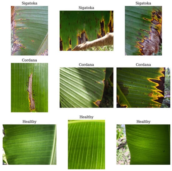
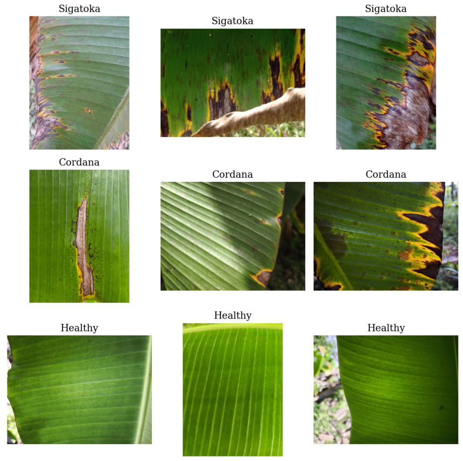
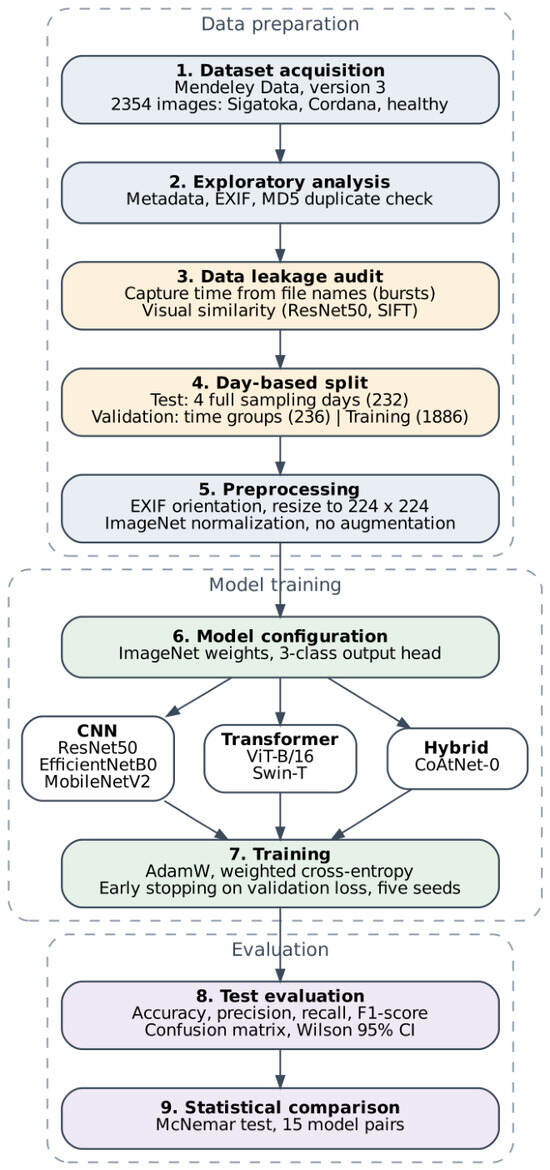
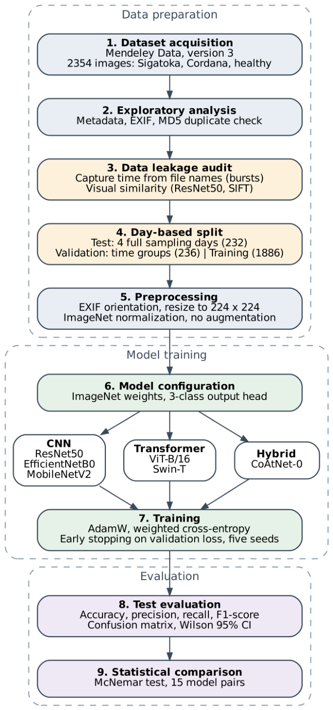
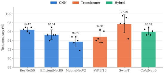
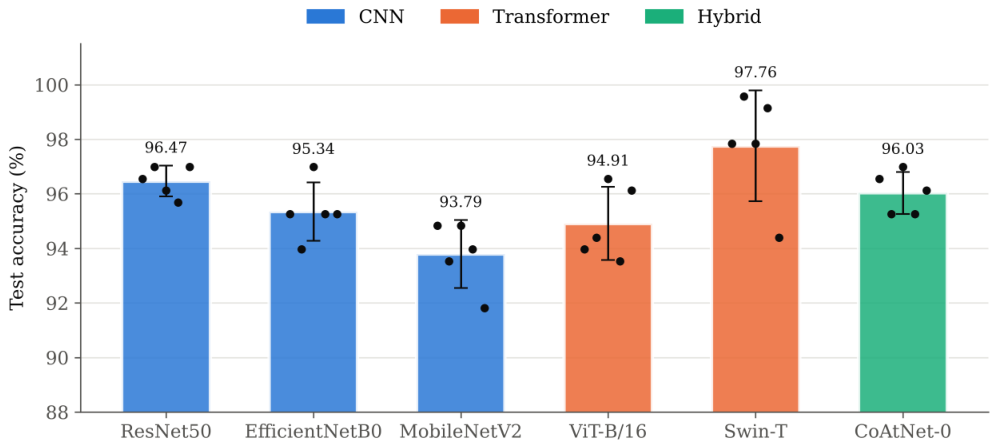
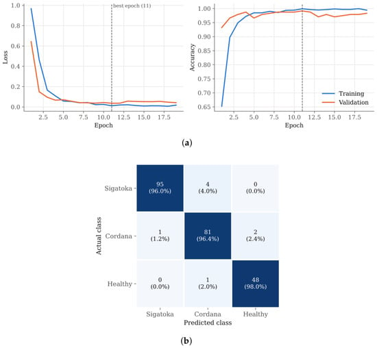
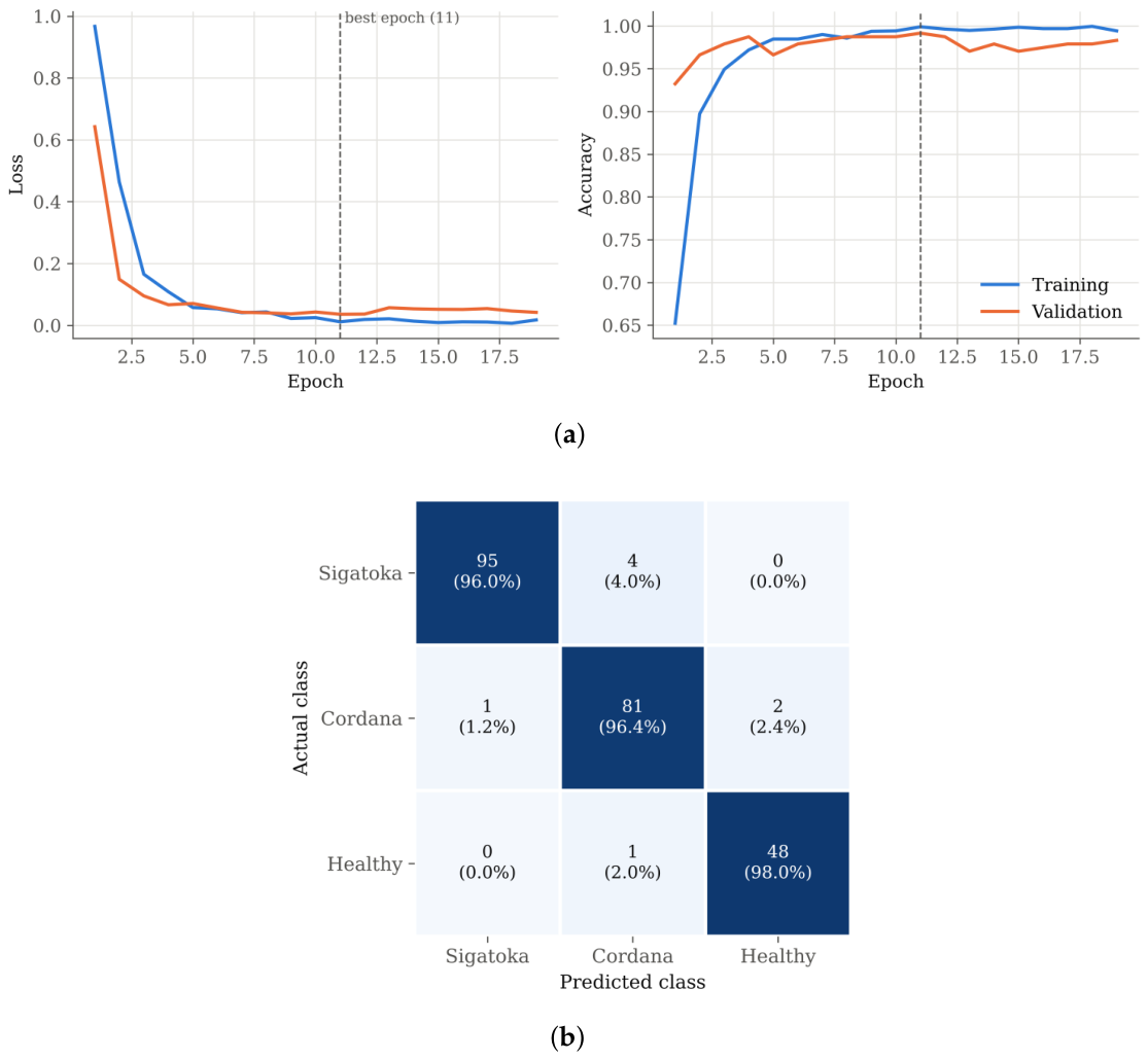
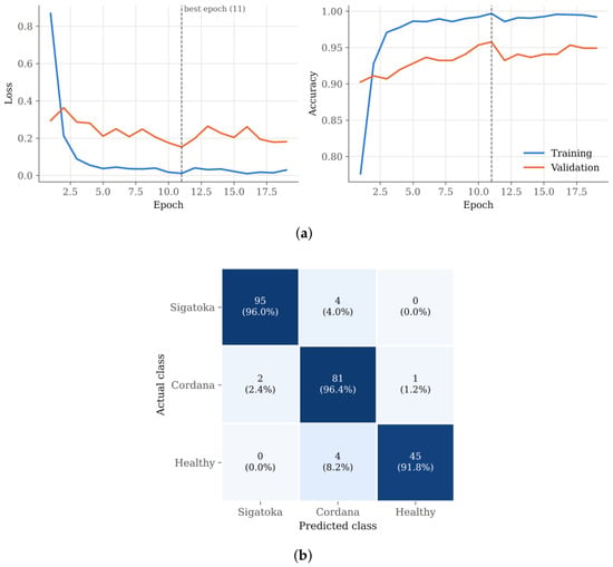
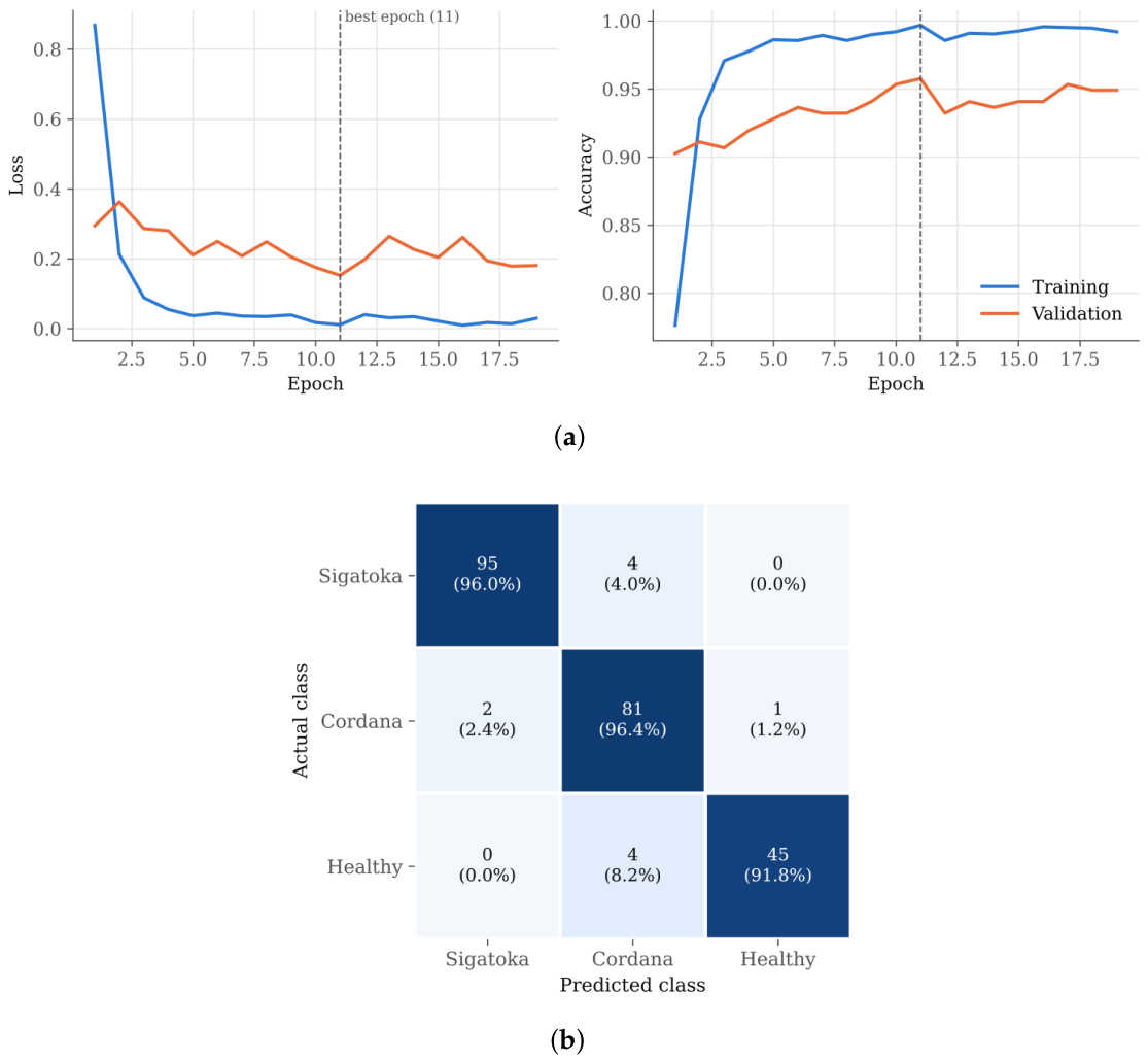
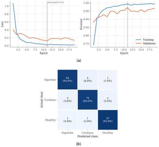
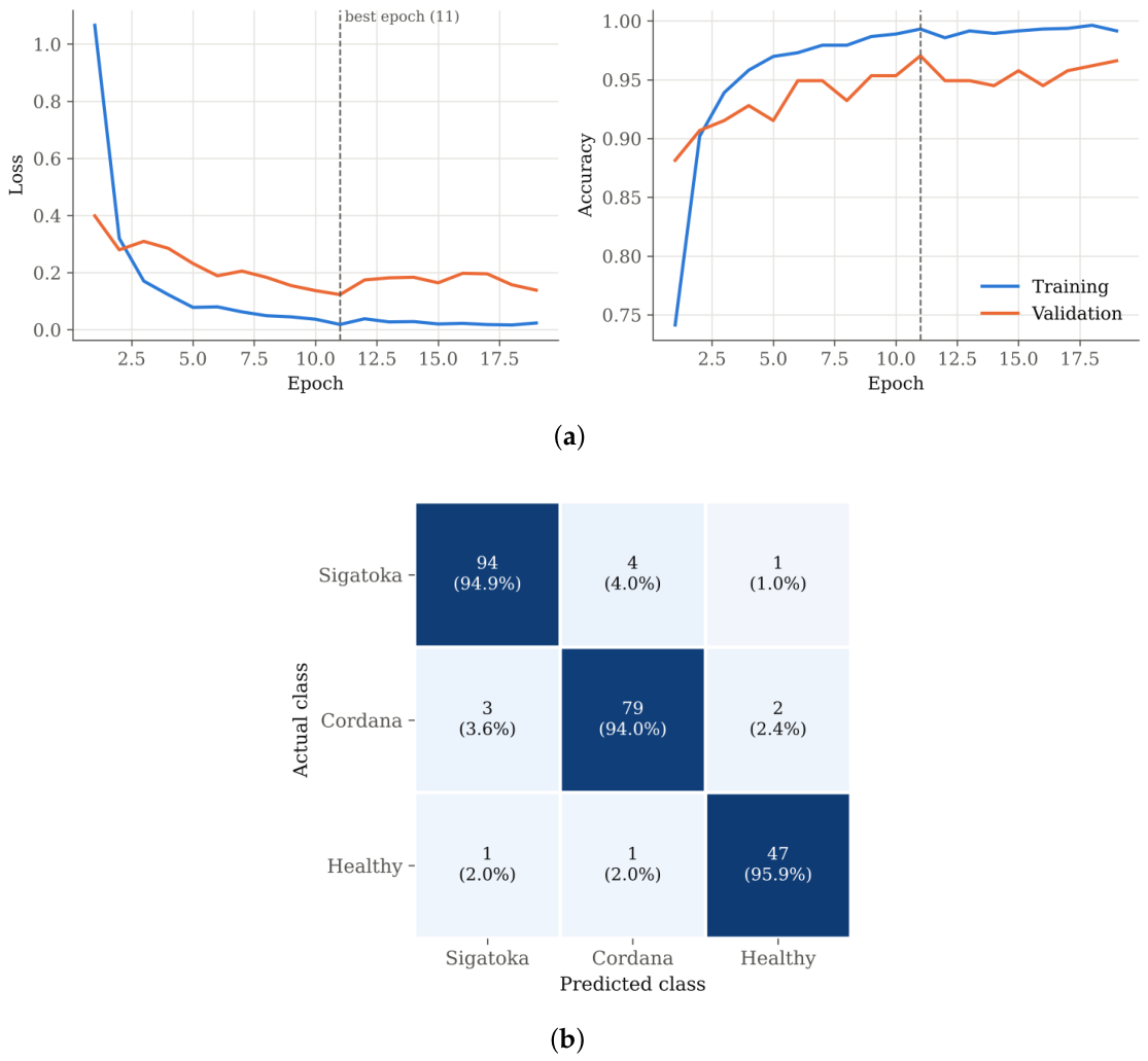
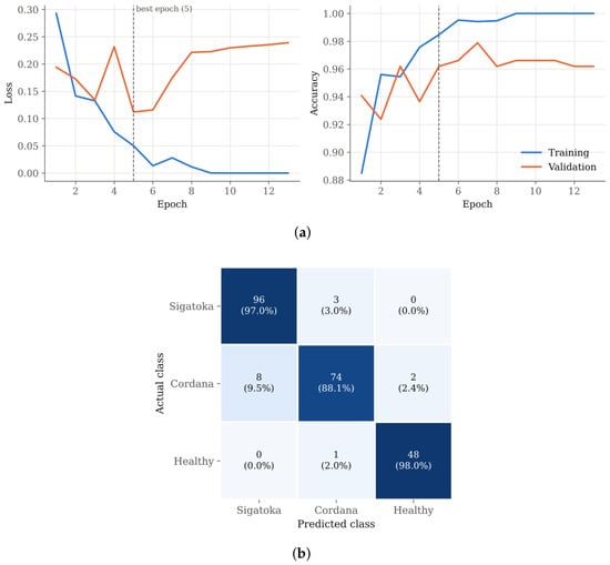
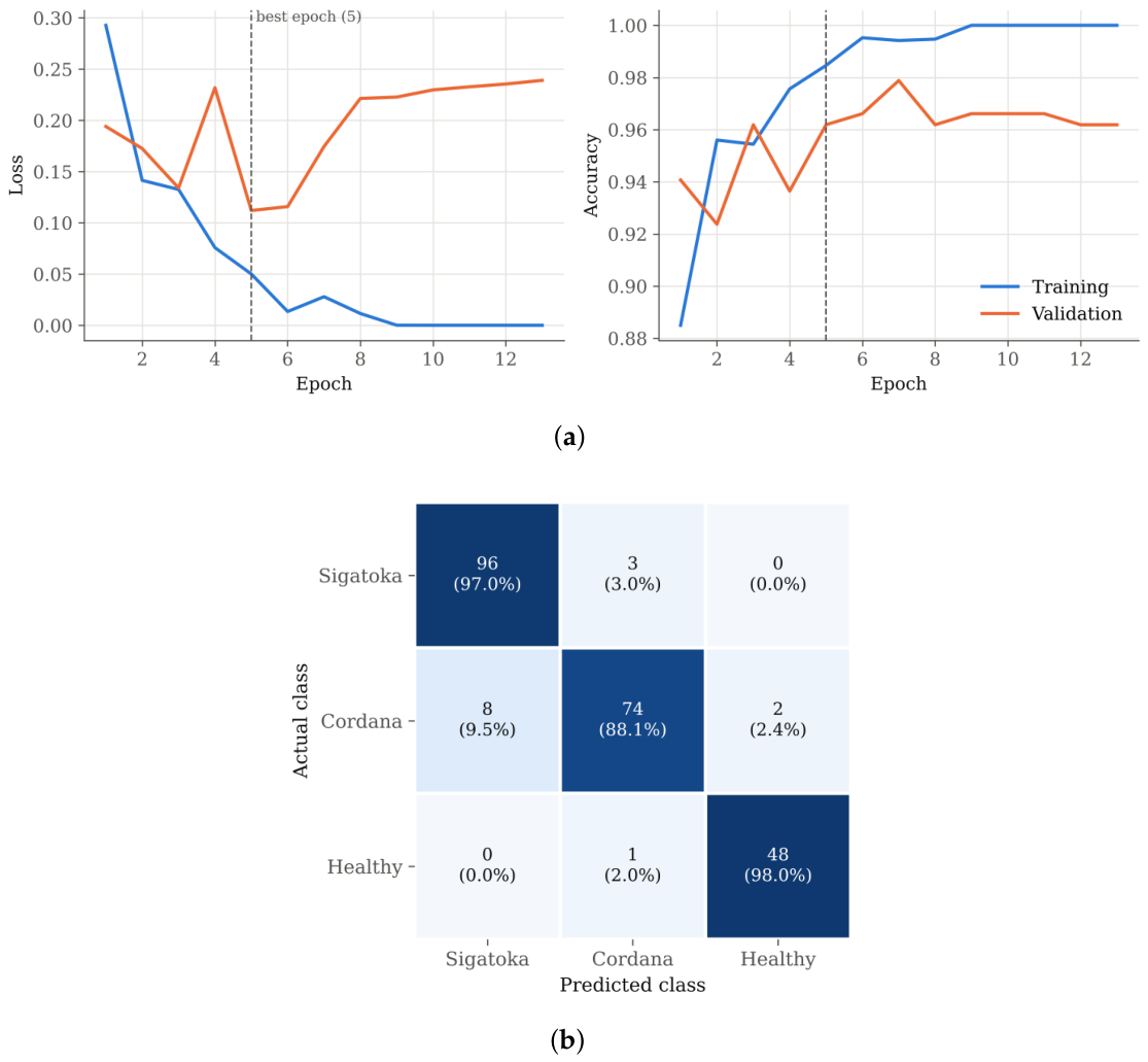
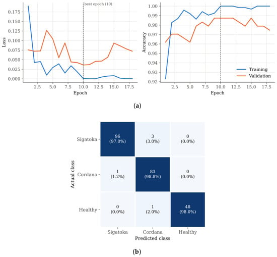
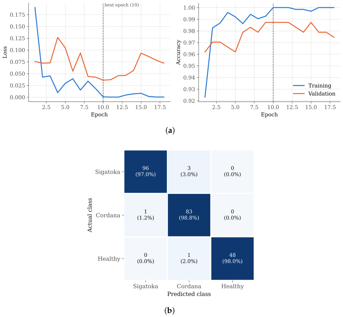
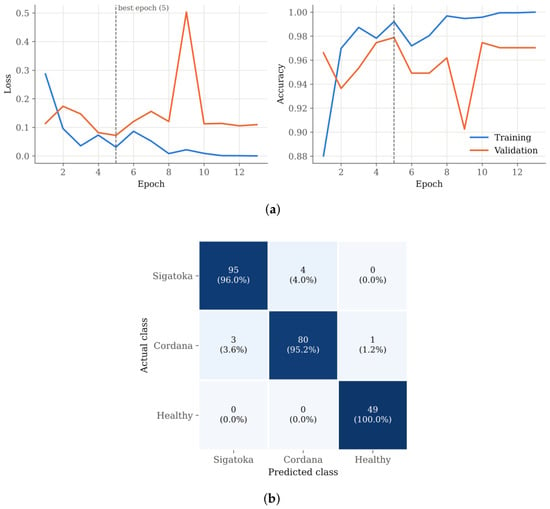
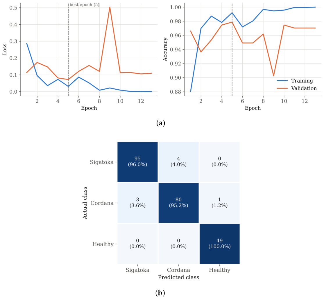
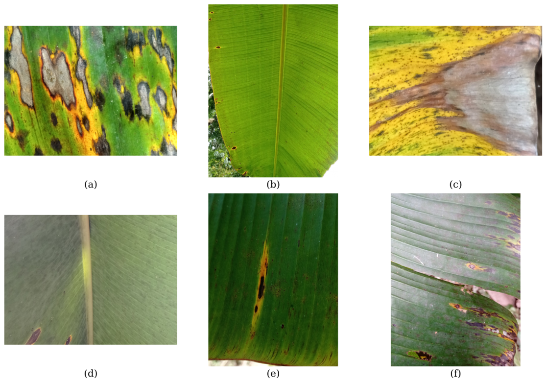

Disclaimer/Publisher’s Note: The statements, opinions and data contained in all publications are solely those of the individual author(s) and contributor(s) and not of MDPI and/or the editor(s). MDPI and/or the editor(s) disclaim responsibility for any injury to people or property resulting from any ideas, methods, instructions or products referred to in the content. |
© 2026 by the authors. Licensee MDPI, Basel, Switzerland. This article is an open access article distributed under the terms and conditions of the Creative Commons Attribution (CC BY) license.