


Abstract
Automatic weed detection represents a tool of interest for precision agriculture and crop monitoring. In this work, the performance of YOLOv8, YOLO11, and YOLO26 was evaluated for the detection of the Foxtail species Cenchrus setaceus and Cenchrus alopecuroides (grouped into a single class), Cortaderia jubata, and Digitaria insularis, due to their presence in Colombia and the large number of images available for their training and evaluation. Images obtained from iNaturalist, Wikimedia Commons, Pl@ntNet and the authors’ own collection were used to construct a dataset of 3156 images. The models were evaluated based on the metrics of Precision, Recall, F1-score, mAP@50, mAP@50-95, and inference speed. The results showed the YOLO26 family remained competitive in each experiment, with the YOLO26s model standing out for both configurations. In addition, the quality and consistency of the dataset labels have a great influence on training efficiency. The results obtained demonstrated the potential of YOLO architectures for the automatic identification of Foxtail species.
1. Introduction
Invasive grasses represent a significant threat to natural ecosystems and agricultural production systems because of their ability to compete for essential resources such as water, nutrients, and solar radiation. They can also alter the composition of plant communities and make management and control activities more difficult [1]. In particular, recent studies have shown that species such as Digitaria insularis can significantly affect the growth and yield of agricultural crops by interfering with physiological, nutritional, and productive variables of cultivated plants [1].
Among the species of interest are Digitaria insularis (sourgrass or capim-amargoso), genus Cortaderia and species of the genus Cenchrus. These species have a high capacity for adaptation and dispersal across different environments. These characteristics favor the colonization of new areas, increase their competitive capacity, and make conventional control strategies more difficult.
Digitaria insularis is considered one of the most problematic weeds in agriculture due to its aggressive competitiveness, excessive seed production, rhizome formation, resistance to herbicides in some cases, and its great capacity to affect crop yield without requiring a high density of the species in the field. For example, in bean crops, yield reductions of 69% were recorded under high infestation conditions [2].
Among the genus Cortaderia, both Cortaderia selloana and Cortaderia jubata have been documented as invasive species. Cortaderia selloana is an invasive species with a high colonizing capacity. This species shows high tolerance to adverse environmental conditions such as drought, temporary flooding, and soils with low resource availability [3,4].
The Global Invasive Species Database (GISD) describes Cortaderia jubata, or jubata grass, as a threat to ecosystems. Even when found at low density, its large size allows it to take light, moisture, and nutrients from other plants, as well as increasing the probability of fires by generating dry biomass [5]. The California Invasive Plant Council (Cal-IPC) includes both C. jubata and C. selloana in its list of high-impact invasive plants [6], as does Oregon State University, which classifies them as invasive perennial grasses [7]. For this study, C. jubata was selected as the representative species of the genus Cortaderia.
Similarly, species related to the genus Cenchrus show a notable capacity for adaptation and expansion due to their efficient seed production and dispersal, which facilitates the establishment of populations in different types of ecosystems outside their original distribution area, causing them to successfully compete with other plant species in most cases.
Although these species belong to different genera, they share similar morphological characteristics, particularly the presence of elongated and feathery inflorescences, commonly associated with the common name “Foxtail”. This visual similarity makes their automatic identification difficult in real environments, especially when there are variations in lighting, plant scale, orientation, and background complexity.
Several studies have explored the use of YOLO for real-time weed detection. Hassan Raza et al. [8] conducted a comparison between models from different YOLO versions, from YOLOv3 to YOLO11, including variants of different sizes such as nano (n), small (s), medium (m), large (l), and extra large (x). The authors found that larger models, such as YOLOv11x, achieve higher detection rates, while lightweight architectures, such as YOLOv8n, achieve shorter inference times.
Likewise, Zheng L. et al. [9] proposed an optimized and lightweight version for weed detection in cotton crops. The authors modified the backbone and C2f module using Star Blocks to improve its inference speed and information capture capability. Consequently, the model reduced the number of parameters and computational cost while maintaining good performance, with mAP@50 and mAP@50–95 values of 98.0% and 95.4%, respectively.
Similarly, Ameer H. Al-Ahmadi et al. [10] explored the use of agricultural robotics and YOLOv5 models for the development of an intelligent variable-rate herbicide application system. Their proposal integrates automatic weed detection with a sprayer system, obtaining precision, recall, and accuracy values above 90% using YOLOv5s. The results demonstrated the feasibility of implementing lightweight models in embedded systems oriented toward real-time agricultural applications.
Additionally, recent studies have investigated the impact of data augmentation techniques on the performance of the model. Baihe Liang et al. [11] proposed an approach based on nine techniques applied to YOLOv9 models for weed and soybean seedling detection. Among the techniques used, Dense Mosaic Augmentation stood out, a variation of the traditional mosaic technique where the focus is on regions with a higher concentration of labels, increasing the model metrics.
Fengying Dang et al. [12] used the CottonWeedDet12 dataset, composed of 12 weed classes, to evaluate the impact of data augmentation techniques on YOLOv3, YOLOv4, and YOLOv5. The transformations performed included rotations, flips, noise, compression, blurring, and brightness variations. The results suggest a better overall performance of the models [12].
On the other hand, Jyostna J. et al. [13] proposed a hybrid approach that combines the detection capability of YOLOv5 with the classification capability of DenseNet, based on convolutional neural networks (CNNs). The system used achieved an mAP close to 92%, effectively distinguishing between crops and weeds.
In other studies, the performance of YOLO has been compared with other machine learning and deep learning models. Vikashini G. et al. [14] evaluated the SVM, ANN, RCNN, and YOLOv9 algorithms for weed detection in zucchini crops in India. The results showed that YOLOv9 achieved an accuracy of 98.213%, outperforming ANN (92.08%), SVM (95.1%), and RCNN (97.06%).
Habib M. et al. [15] compared the effectiveness of optimizing the backbone of a YOLOv5 model with MobileNetV1. The study highlighted the ability of the YOLO model to maintain a balance between accuracy and inference speed, as well as its stability under variations in the Intersection over Union (IoU) threshold, showing high effectiveness when delineating weeds in complex scenarios.
2. Materials
2.1. Dataset
The dataset used in this study was built with images of 4 weed species commonly named as Foxtail. The images were obtained using inat_downloader, a Python 3.14 script that allows downloading images and metadata from iNaturalist [16]. For image collection, inat_downloader allows configuring it to only download those with usage licenses. Additional images of Digitaria insularis were obtained from Wikimedia Commons and Pl@ntNet, with the corresponding attribution and usage licenses recorded for each image. A small number of images were also obtained directly by the authors.
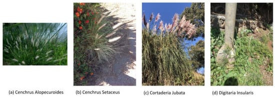
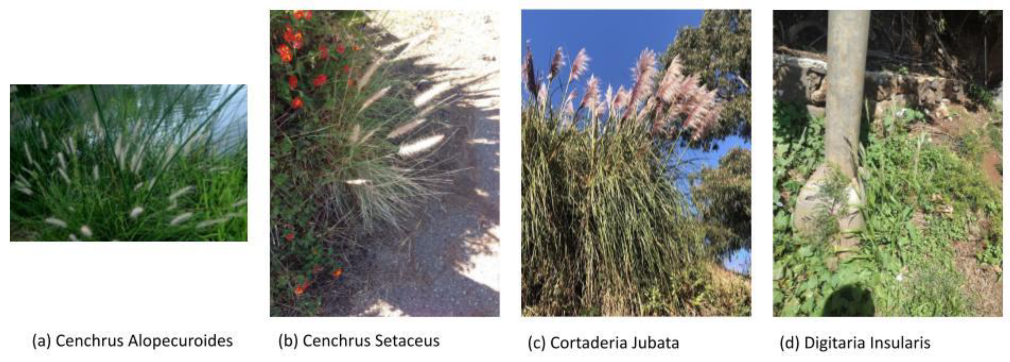
The species used were Cenchrus setaceus, Cenchrus alopecuroides, Cortaderia jubata, and Digitaria insularis. Images of Cenchrus setaceus and Cenchrus alopecuroides were grouped into a single class called Cenchrus. After the image selection process, the dataset contained 661 images: 250 corresponding to Cenchrus, 252 to Cortaderia jubata, and 159 to Digitaria insularis. The dataset was randomly divided using Roboflow into training, validation, and test sets using a 75%, 15%, and 10% split, respectively, resulting in 499 training images, 96 validation images, and 66 test images. We can observe examples of the images used for the dataset in Figure 1.
Figure 1.
Example of species used for the dataset. (a) Cenchrus alopecuroides [17]; (b) Cenchrus setaceus [18]; (c) Cortaderia jubata [19]; (d) Digitaria insularis [20].
The images presented variability in terms of scale, background, illumination, and plant orientation. The selection process focused on images where the complete plant could be observed. In cases where only part of the plant structure was visible, the image was retained if the visible portion corresponded to the tiller of the plant, whereas images focused mainly on the inflorescence were excluded from the dataset. When possible, images containing more than one plant were preferred to increase the variability of the scenes. Images where the plant occupied the whole frame were discarded. However, some images in which the plant occupied a considerable portion of the frame were retained to represent plants located close to the camera, as this type of viewing condition may be relevant to a future mobile platform equipped with a camera.
When multiple images originated from the same observation event, their visual similarity was considered during image selection. Images from the same observation that showed sufficiently different positions or viewing angles of the plant were included in the dataset.
This study only focuses on the analysis of the detection performance of the complete plant and three-class detection based on species groups. For this, two configurations of the dataset were made according to their respective task:
- (i)
- Whole-plant detection (a single class: “Foxtail”);
- (ii)
- Three-class detection using Cenchrus, Cortaderia jubata, and Digitaria insularis.
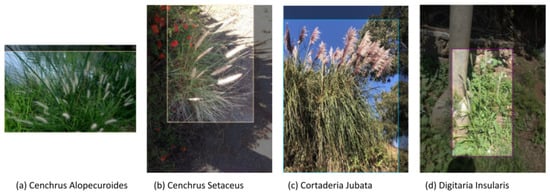
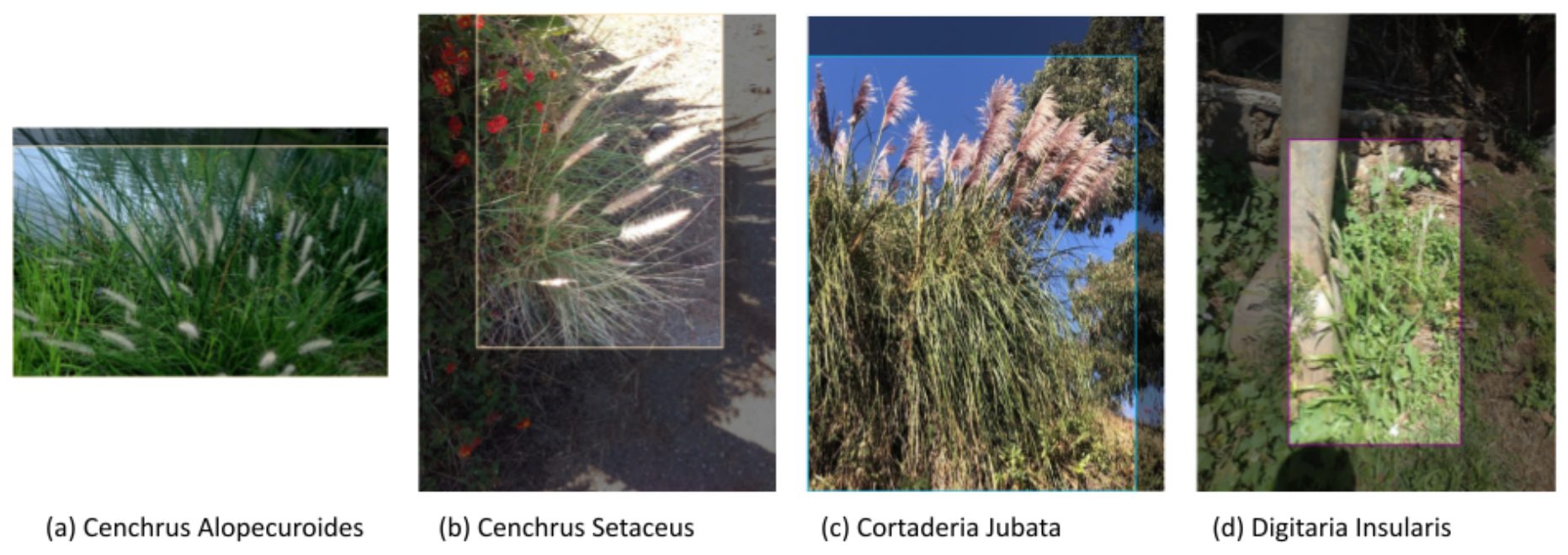
For configuration (ii), the species Cenchrus alopecuroides and Cenchrus setaceus were grouped into a class named Cenchrus, due to their high morphological similarity and lower number of images available of Cenchrus alopecuroides. This was done with the purpose of reducing class imbalance that can cause biases during training. Some examples of the annotations made can be observed in Figure 2.
Figure 2.
Examples of class labels in the dataset: (a) Cenchrus, based on the photograph in [17] (b) Cenchrus, based on the photograph in [18]; (c) Cortaderia jubata, based on the photograph in [19]; (d) Digitaria insularis, based on the photograph in [20].
The bounding boxes were manually defined by the second author following a consistent criterion for whole-plant detection. For tussock-form plants, the bounding box included the visible base of the plant or clump and extended to include the visible inflorescences associated with the plant. When the inflorescence was not visible, the annotation was based on the visible portion of the plant or tiller. When multiple plants or clumps could be visually distinguished, they were annotated as separate instances, while dense clumps in which individual plants could not be reliably distinguished were annotated as a single instance. Images were selected and annotated according to the visibility of the plant and the possibility of defining its boundaries.
After the initial annotation process, the images were randomly distributed among the training, validation, and test subsets. A manual quality-control review was then conducted by the second author. This process checked class-label consistency, bounding box placement, the inclusion of clearly distinguishable plant instances, duplicate annotations, and compliance with the image selection and annotation criteria described above. Images originating from the same observation were also checked to ensure that they remained within the same data split, preventing data leakage between training, validation, and test sets. When images were removed during this review, they were replaced as needed to maintain the original proportions of the subsets. All identified annotation and distribution errors were corrected before the final evaluation.
Initially, the three-class configuration (ii) was labeled, and then copied to create a second dataset corresponding to configuration (i), where the three classes were renamed to the single class “Foxtail”. This allowed direct comparison between the two detection tasks, as they differed only in the class configuration used for training and evaluation.
The final datasets, including image-level attribution and information on the original licenses of third-party images, are available through Roboflow Universe: single-class dataset and three-class dataset. The accompanying README files document the attribution and original license information for individual images. The CC BY-NC-SA 4.0 license associated with the datasets does not supersede the original license terms applicable to third-party images.
2.2. Data Augmentation and Preprocessing
Prior to model training, a preprocessing and data augmentation process was performed with the aim of improving generalization capability and mitigating the limitations arising from the reduced dataset size. Data augmentation was applied only to the training set, while the validation and test sets remained unchanged.
All transformations were implemented using the Albumentations library. Each original training image was used to generate five augmented versions. The same augmentation pipeline and parameters were used for both dataset configurations independently but maintaining the same transformation pipeline and parameters. Since these transformations are random, the augmented images could differ between configurations, even though they were generated from the same original training images.
The augmentation pipeline included horizontal flipping with a probability of 0.5 and rotations within a range of −10° to 10°, also with a probability of 0.5. Brightness variations of ±15% were applied with a probability of 0.5, while the contrast was kept unchanged. An affine transformation was used to simulate zoom-out conditions, with a scale ranging from 0.75 to 0.95 and translations of up to ±5% of the image dimensions. Gaussian noise was applied with a probability of 0.2 using a low-intensity range, and Gaussian blur with a 3 × 3 kernel was applied with a probability of 0.15. Finally, all images were resized to a uniform resolution of 640 × 640 pixels following the configurations commonly used in Ultralytics-based YOLO models [21].
This significantly increased the number of samples available for training. As a result, each dataset configuration contained 3156 images, including 2994 training images, 96 validation images, and 66 test images. Therefore, the final distribution was 94.87% for training, 3.04% for validation, and 2.09% for testing.
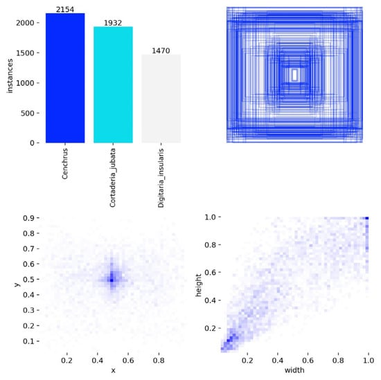
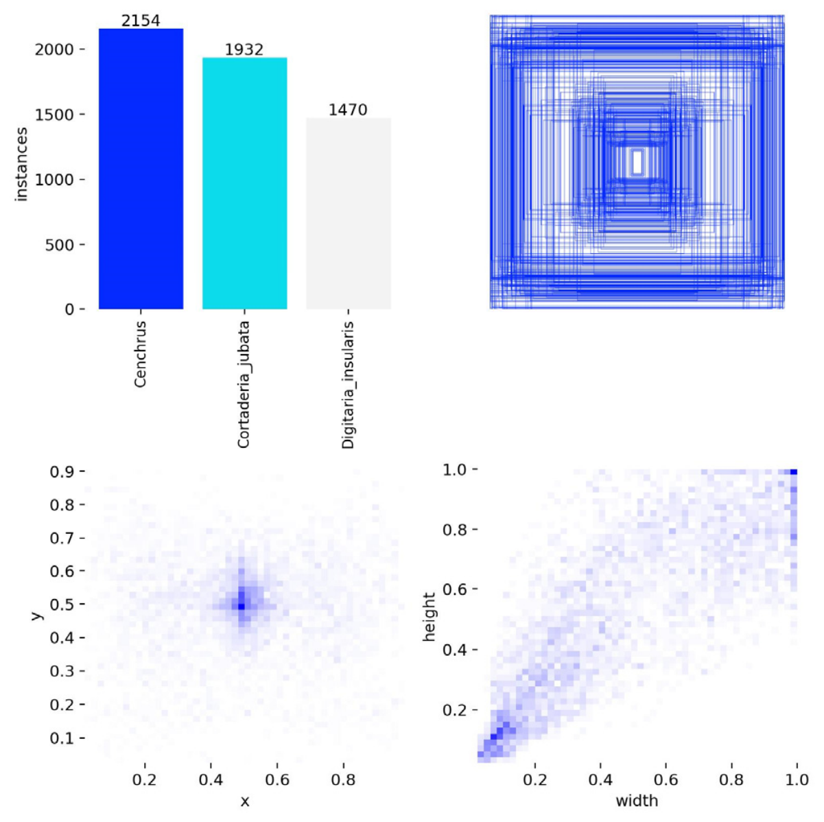
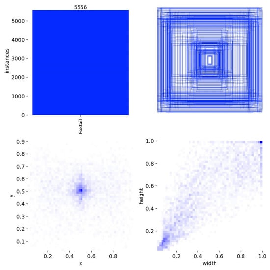
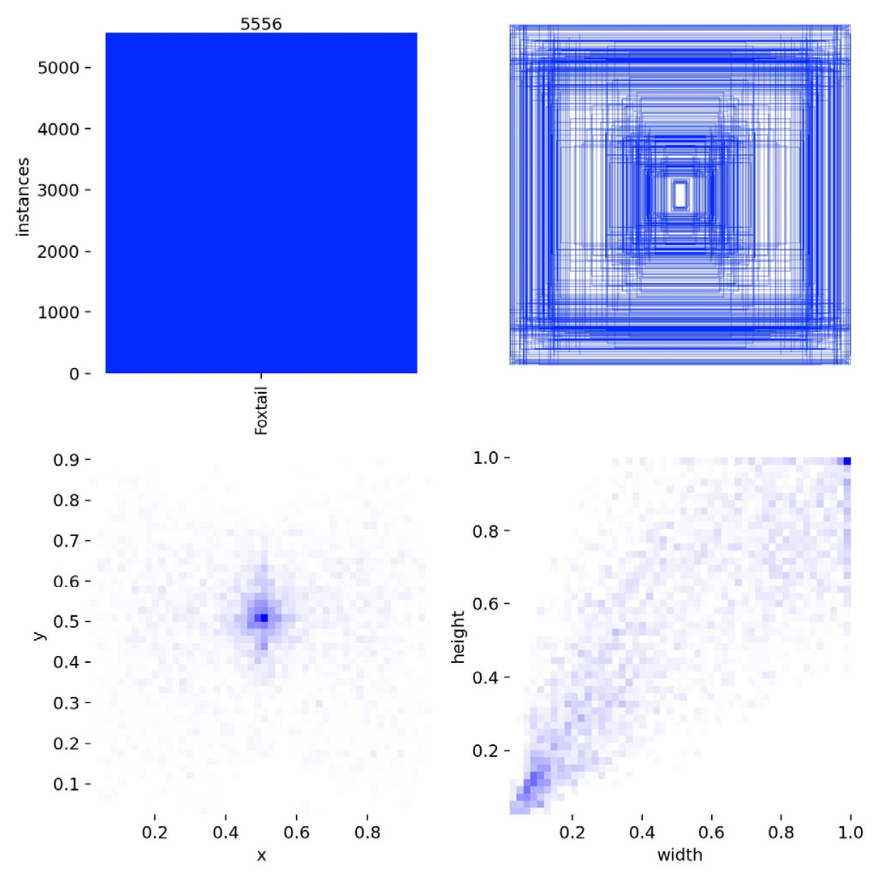
For Figure 3 and Figure 4, the spatial distribution, size, and number of instances of each configuration can be observed ((i) and (ii), respectively). As the second dataset corresponds to the same annotations as the first one, but renamed and retaining the same augmentation pipeline, the sum of the instances in Figure 3 is consistent with the total in Figure 4. However, as mentioned previously, since the augmentations are random, the generated labels will be different, as can be observed in the distribution of the bounding boxes in the images. Although the change is minimal, it is present, as well as a slightly different spatial and size distribution between both configurations.
Figure 3.
Three-class configuration labels: (top-left) number of instances per class; (top-right) distribution of bounding boxes in the image; (bottom-left) spatial distribution of the centers of the annotations; (bottom-right) distribution of the width and height of the bounding boxes.
Figure 4.
Single-class configuration labels: (top-left) number of instances per class; (top-right) distribution of bounding boxes in the image; (bottom-left) spatial distribution of the centers of the annotations; (bottom-right) distribution of the width and height of the bounding boxes.
It can be observed that most of the labels are centered. This may be because iNaturalist and the other sources used provide photographs in which plants can be clearly observed, often with framing focused on the plant itself. This can lead to problems such as low positional variability, despite the displacement augmentations that were performed. A difference can also be observed in the number of instances associated with the species Digitaria insularis, which may contribute to an imbalance between the classes and affect the training process.
2.3. Model Architecture
YOLO26 is the most recent version of the YOLO family developed by Ultralytics. It focuses on real-time object detection and optimization for edge devices and fast execution on CPU. This model aims to provide a balance between inference speed and precision, resulting in a fast model with low computational cost and less dependence on a GPU.
Some of the changes made for this version include producing a direct final detection by eliminating Non-Maximum Suppression (NMS) to discard duplicate boxes in order to reduce latency. To simplify the inference process, Distribution Focal Loss (DFL) is no longer used; instead, a direct bounding box prediction process is used. It also incorporates STAL (Small-Target-Aware Label Assignment), a technique designed to improve the detection of small objects by preventing them from being ignored during training. According to Priyanto Hidayatullah et al. [22], the model can achieve CPU inference speeds 43% higher compared to some previous versions.
To evaluate the performance of this architecture for invasive grass detection, YOLOv8 and YOLO11 were selected as reference models because they are widely used in similar computer vision tasks in the field of smart agriculture.
YOLOv8 was included because of its wide use in weed and crop detection. Studies such as [23,24,25] proposed modifications to the architecture to increase its efficiency in the field of agriculture, demonstrating its effectiveness as a reference model for this type of application.
Similarly, YOLO11 has been showing competitive results in terms of detection capability and computational cost. Studies such as [26,27] highlight its potential for computer vision tasks, which is why it was selected as the second model for comparison.
For an objective evaluation, the Nano (n), Small (s), and Medium (m) variants of the three families were used for comparison. These were trained using the same dataset and training hyperparameters, enabling a comparison of the performance of each model under consistent experimental conditions.
2.4. Training Configuration
Table 1 shows the hyperparameter configuration used for training the models. This configuration was used for each variant to ensure an objective evaluation.
Table 1.
Main hyperparameters used during the training of the YOLO models.
As shown in Table 1, the models were trained for 300 epochs using an image size of 640 × 640 pixels and a batch size of 32 samples. A Cosine Learning Rate Scheduler was used alongside an initial learning rate of 0.001. To avoid overfitting, a dropout of 0.2 and early stopping with a patience of 50 epochs were configured. Additionally, pretrained weights, automatic mixed precision (AMP), disk caching, and the AdamW were used as the optimizer. Finally, random seeds of (0, 41 and 123) were used together with deterministic training to ensure reproducibility of the results.
2.5. Hardware and Software Environment
In Table 2, we can observe that the training was performed on the Windows 11 operating system, equipped with an AMD Ryzen 9 9950 (Advanced Micro Devices, Inc., Santa Clara, CA, USA) × 3D processor, 128 GB of RAM, and an NVIDIA GeForce RTX 5080 GPU. An NVIDIA graphics card was selected due to its CUDA support and compatibility with PyTorch and Ultralytics YOLO, allowing faster training thanks to the parallel processing offered by the GPU. The software environment consisted of CUDA 13.0, PyTorch 2.11.0 + cu130, and Ultralytics 8.4.48, ensuring compatibility between the tools used for model training.
Table 2.
Specifications of the experimental environment.
2.6. Statistical Analysis
Each architecture was trained using the three random seeds specified in Table 1 to account for the variability introduced during the training process. Once the training was completed, the best model from each run was selected, and the mean and standard deviation (SD) were calculated for each architecture. Therefore, the values reported in the tables are presented as mean ± SD.
This analysis was applied to the evaluation metrics, including precision, recall, mAP@50, mAP@50–95, and F1-score, as well as to the inference speed analysis performed for each model trained with each seed. This approach provides a more representative description of the performance of each architecture by accounting for the variability introduced during the training process.
2.7. Inference Speed Benchmark
For this study, two procedures were performed to evaluate the inference speed of each model. Initially, the inference time data obtained from the model.val() function of Ultralytics were used, which allows the performance of the trained model to be measured on the validation set. An input resolution of 640 × 640 pixels and a batch size of 32 were used. This Ultralytics function provides the preprocessing, inference, and postprocessing times, whose sum was used to calculate the FPS.
Subsequently, a benchmark was performed with a batch size of 1 using a single image from the validation set. Before the measurements, 50 warm-up predictions were performed to avoid the effect of initial execution overhead, followed by 200 predictions that were timed for each model and subsequently averaged to calculate the FPS. This procedure was performed for both CPU and GPU. For the GPU, CUDA synchronization was performed before and after each prediction to ensure that the measured times were correct.
2.8. Evaluation Metrics
To measure the performance of the models used, the metrics Precision, Recall, F1-Score, and mAP@50 will be evaluated.
Precision allows measuring the percentage of correct predictions from the total number of inferences made by the model:
where corresponds to the true positives and to the false positives.
Recall measures the percentage of instances that were detected from the total number of objects present in the image:
where represents the false negatives.
F1-Score combines Precision and Recall through a harmonic mean, being a useful metric to measure the model’s ability to avoid false detections and the omission of instances:
Intersection over Union (IoU) allows evaluating the quality with which the model locates and delimits the object compared to the original label:
where corresponds to the bounding box predicted by the model and to the ground-truth annotation.
Average Precision (AP) measures the area under the Precision-Recall curve, allowing the model’s performance to be summarized through different confidence thresholds. An AP value close to one indicates that the model simultaneously maintains high levels of precision and recall across different decision thresholds.
where represents precision as a function of recall.
The mAP@50 and mAP@50-95 metrics allow measuring the Average Precision (AP) using different IoU thresholds. For mAP@50, a threshold of 0.5 is considered, while mAP@50-95 evaluates different thresholds from 0.5 to 0.95, allowing the model’s performance to be evaluated under stricter localization conditions.
To facilitate the interpretation of the training and validation curves, an exponential moving average (EMA) filter was applied to the metrics recorded at each training epoch. This filter smooths short-term fluctuations and allows a general trend of the training behavior of each model to be observed.
The exponential moving average used to smooth the curves is defined as:
where represents the smoothed value at time , corresponds to the original metric, is the smoothed value from the previous step, and is the smoothing factor.
The mean value represents the average performance obtained across the three runs and is defined as:
where represents the mean value, represents the result obtained in each run, and represents the total number of runs.
The standard deviation was calculated to quantify the variability of the results obtained across the three training runs and is defined as:
where represents the standard deviation, represents the result obtained in each run, represents the mean value, and represents the total number of runs.
3. Results
The same hyperparameter configuration presented in Table 1 was used in both experiments to ensure consistent training conditions and enable a controlled comparison of model performance across the evaluated architectures.
The training process was performed three times for each architecture, using a different seed for each run. This allowed the variability in the results across training runs to be evaluated. Subsequently, the mean and standard deviation of the results obtained from the three runs were calculated, providing a more representative summary of model performance and accounting for variability across runs.
Once the training was finished, YOLO generates a results.csv file in which the performance of the metrics in each epoch is saved. Although a maximum of 300 epochs was established, not all models reached this value since the early stopping criterion was used, which stops the training when the validation metrics stop showing significant improvements over the number of epochs defined in the patience parameter. For the evaluation of the model performance, the best checkpoint obtained during training was selected based on the validation results.
To evaluate the model performance, the curves of validation and training metrics were analyzed, especially those showing precision, recall, and mAP. Considering that these metrics show natural fluctuations throughout the training epochs due to the training process, a smoothing process was performed using exponential moving average (EMA) to allow a visualization of the general trend of each model.
A smoothing coefficient of α = 0.1 was used, which reduces the oscillations present in the curves without losing relevant changes during training. This facilitates the comparison between the models and the analysis of their convergence behavior.
Finally, the performance of each model was compared using the final validation metrics on the test set: precision, recall, mAP@50, mAP@50-95, and F1-score. In addition, the metrics related to computational efficiency, such as frames per second (FPS), were considered to evaluate not only their detection capability but also their processing capacity and speed.
3.1. Foxtail Detection
The results of the final metrics are presented in Table 3. No single model was predominant across the evaluated metrics. YOLO26m stood out for achieving the highest precision and F1-score, YOLO26n for recall, YOLO11n for mAP@50, and YOLO26s for mAP@50–95. If the best model is selected based on its ability to correctly localize instances under stricter IoU thresholds, YOLO26s would be the most suitable option, while remaining competitive in terms of mAP@50. However, it presents difficulties in identifying all the instances present compared with the other models, as reflected in its lower recall compared with YOLO26n.
Table 3.
Comparison of final metrics of each model for single-class detection using test split.
In this case, the models stand out for their precision; therefore, fewer background instances are incorrectly detected as foxtail. However, a considerable deficiency can be observed in the mAP@50–95 metric, which decreases by more than 30% in some cases compared with mAP@50. Although most models manage to correctly identify the plants, in several cases they fail to generate bounding boxes that adequately match the corresponding annotations.
The difference between the precision and recall results shows that the main limitation does not correspond to the generation of false detections, but to the inability to detect all the instances present in the images. The relatively high precision indicates that in the cases in which an object is identified as Foxtail grass, it does so correctly. However, the low recall indicates that a considerable proportion of the weeds are not detected.
Additionally, the difference between mAP@50 and mAP@50-95 suggests limitations related to the localization of the predicted bounding boxes, since as the IoU threshold becomes stricter, the model performance decreases. Therefore, the main challenges of this task consist of detecting all the existing instances and accurately localizing the detected objects, rather than the generation of false positives.
To evaluate the inference speed, the procedure described in Section 2.7 was followed. The results obtained for each model are presented in Table 4.
Table 4.
Comparison of FPS measured during Ultralytics validation and benchmarking using CPU and GPU for single-class detection.
The smaller models present a higher number of FPS, especially during Ultralytics validation. YOLOv8n reached 284.05 ± 62.25 FPS on GPU, followed by YOLO11n with 270.30 ± 18.18 FPS and YOLO26n with 216.59 ± 43.37 FPS. On CPU, the models also maintain higher speed in their n configurations, with values of 76.08 ± 1.07 FPS, 73.25 ± 0.65 FPS, and 72.90 ± 2.69 FPS for YOLOv8n, YOLO11n, and YOLO26n, respectively. The benchmark showed a similar behavior regarding the effect of model size, although the FPS values were different from those obtained during Ultralytics validation. This confirms the need to consider the measurement procedure when comparing inference speed. In addition, the standard deviations were higher in some GPU measurements for the n models, while the CPU measurements presented lower variability.
One of the proposals of YOLO26 is to optimize inference speed, especially for predictions performed on CPU. In this experiment, YOLO26 is able to compete with YOLO11, maintaining similar averages and even lower values in some cases. However, the differences observed between YOLO26 and YOLO11 are not large enough to establish a clear advantage in inference speed.
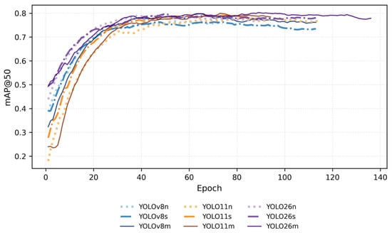
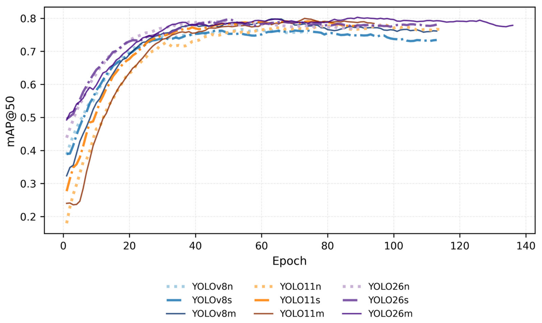
For the evaluation of the metrics by epochs, a representative model of each trained architecture was added. This was selected by looking for the model whose metrics were closest to the standard mean presented in Figure 5, thus allowing the performance of each model to be evaluated. It should be noted that these graphs do not represent the progress of the three seeds, but rather that of the seed that showed the highest agreement with the final metrics, as mentioned previously. The filter used to smooth the graphs was the previously mentioned EMA; therefore, the graph may not exactly match the value recorded in the table, since it should be remembered that the table presents the mean of the three seeds, while the graph shows the smoothed trend of a single run.
Figure 5.
Comparison of model performance in the Foxtail detection task, evaluating the behavior of the mAP@50 metric.
In Figure 5, it can be observed that the models present a progressive increase in mAP@50 during the initial stages of training. Although YOLOv8n begins to decrease from approximately epoch 50, most of the models tend to remain more stable throughout the epochs. Among those evaluated, the YOLO26m, YOLO26s and YOLO11m reach convergence with higher values. For the rest, no clear relationship was found between model size and performance. It is important to emphasize that this graph does not represent the final values reported in Table 3. Although the mentioned models showed more favorable trends, they did not achieve the highest mAP@50 values. Additionally, the training behavior across epochs shown corresponds to the run, among the three runs selected for each model, whose results were closest to the mean values reported in the tables.
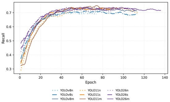
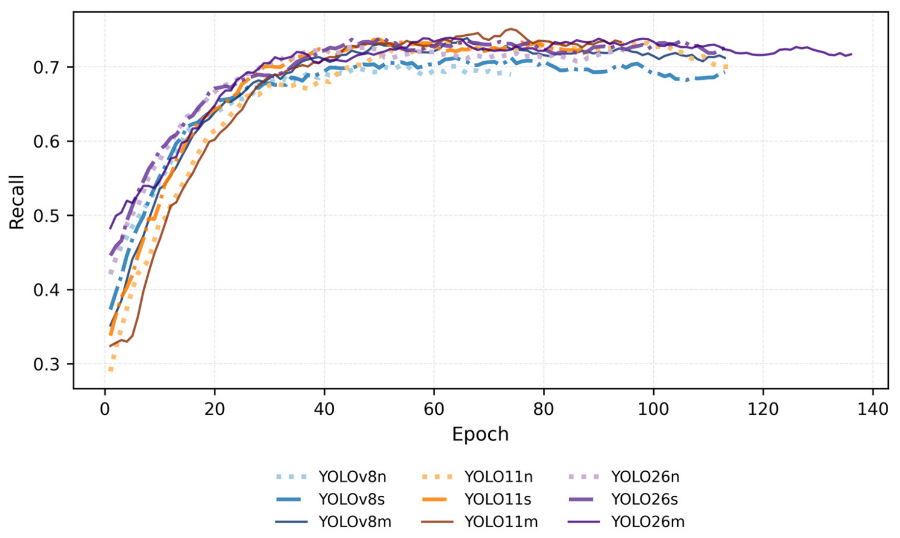
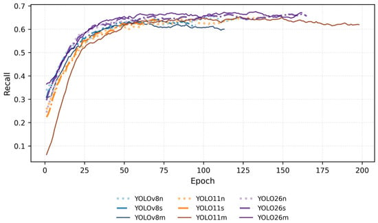
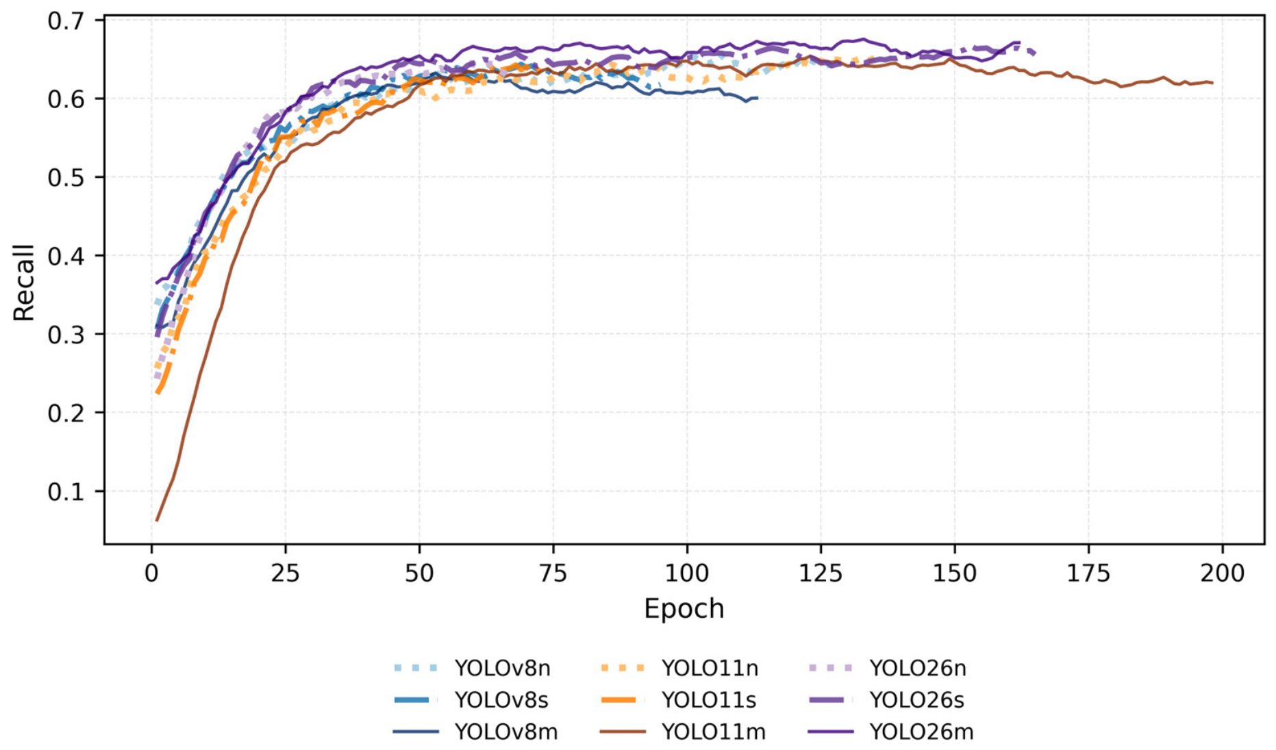
Figure 6 allows us to see the evolution of recall during training. This metric shows greater variability during training compared to mAP@50. As mentioned previously, recall represents one of the main difficulties present in this model, since even during later stages some models continue to show oscillations. In most epochs, the models maintain a recall above 0.7. Although some models show a decrease toward the end, they manage to maintain an acceptable recall trend. However, YOLOv8n and YOLOv8s were the models that remained closest to 0.7. It was also observed that the m models maintained slightly more stable performance before decreasing, as occurred with the other models, with YOLO26m sustaining this behavior for a greater number of epochs.
Figure 6.
Comparison of model performance in the Foxtail detection task, evaluating the behavior of the Recall metric.
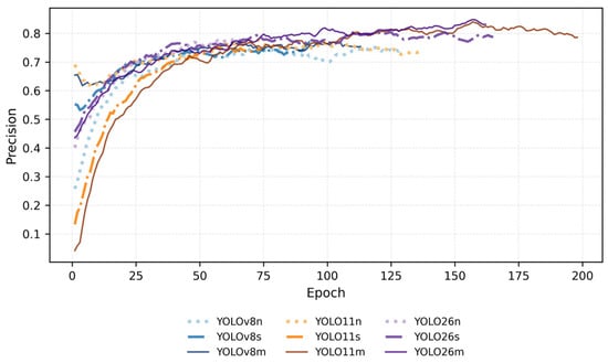
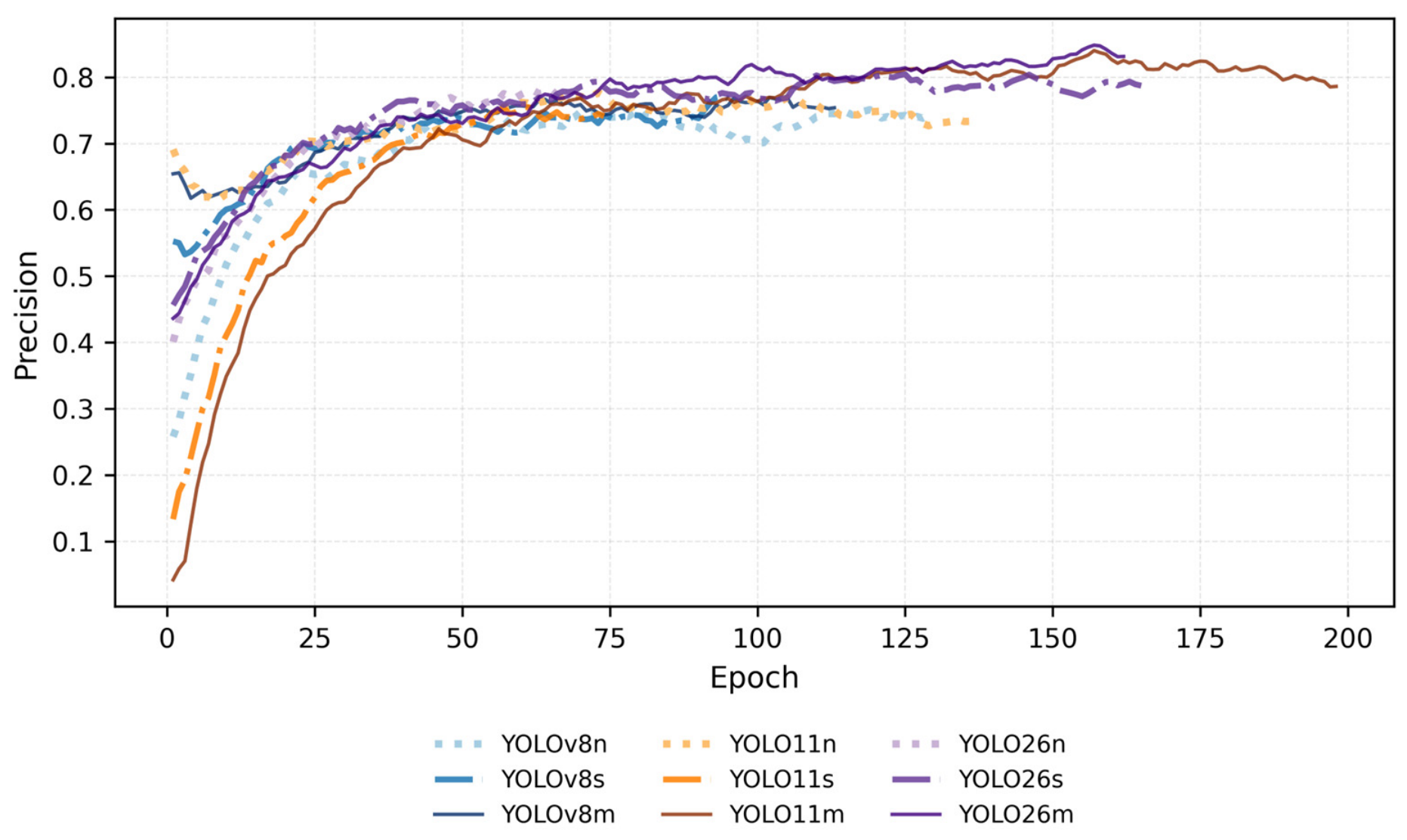
Regarding precision (Figure 7), in this graph, a constant growth can be observed in all the models, generally surpassing a precision of 0.8. This allows us to determine that the models tend to learn over time and improve their ability to avoid false positives.
Figure 7.
Comparison of model performance in the Foxtail detection task, evaluating the behavior of the Precision metric.
In this case, a more favorable trend was observed for the selected YOLO26n model, which was eventually matched by YOLO26m, as it continued training for more epochs and achieved similar values. However, although YOLO26m achieved the highest precision, YOLO26n presented an average precision that was about 5.8% lower, with a variation in the precision of the model of only 0.001. Ultralytics selects the best model based on the mAP metrics. Therefore, achieving high precision values does not necessarily indicate that a model will be the best overall, since other metrics must also be considered, such as recall and its ability to accurately localize each instance.
Overall, the results show a favorable general performance of YOLO26s for the Foxtail detection task.
3.2. Three-Class Detection
The results presented in Table 5 show differences between the models depending on the metric evaluated. In precision, YOLO26n stands out with 0.876, followed by YOLO26m with 0.849, while in recall, YOLO26m presents the highest value with 0.807, followed by YOLO11m with 0.773. For F1-score, YOLO26m stands out with 0.826, followed by YOLO26n with 0.818. In mAP@50, YOLO26n obtains the highest value with 0.839, followed by YOLO26m with 0.831, and in mAP@50–95, YOLO26m again presents the highest result with 0.509, followed by YOLO26n with 0.493. Therefore, YOLO26m and YOLO26n were the models that stood out in most of the evaluated metrics.
Table 5.
Final metrics for each model for three-class detection using the test split.
The FPS results recorded in Table 6 showed considerable differences depending on the measurement method and hardware used. YOLOv8 was not consistently the fastest family when compared with the other architectures of their respective sizes. During Ultralytics validation, YOLOv8n achieved the highest GPU speed with 351.337 ± 148.006 FPS, followed by YOLO26n with 336.423 ± 126.922 FPS and YOLO11n with 299.233 ± 9.765 FPS. However, these results were accompanied by high standard deviations, especially for YOLO26n and YOLOv8n. On CPU, YOLOv8n also achieved the highest speed with 77.073 ± 0.629 FPS. In the benchmark, YOLOv8n again presented the highest values on both GPU and CPU, with 176.730 ± 13.685 FPS and 90.600 ± 1.367 FPS, respectively. The n-sized models achieved higher FPS, with YOLOv8 being the fastest in most measurements. However, there was no consistent difference in speed between YOLO26 and YOLO11 when comparing models of the same size.
Table 6.
Comparison of FPS measured during Ultralytics validation and benchmarking using CPU and GPU for three-class detection.
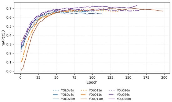
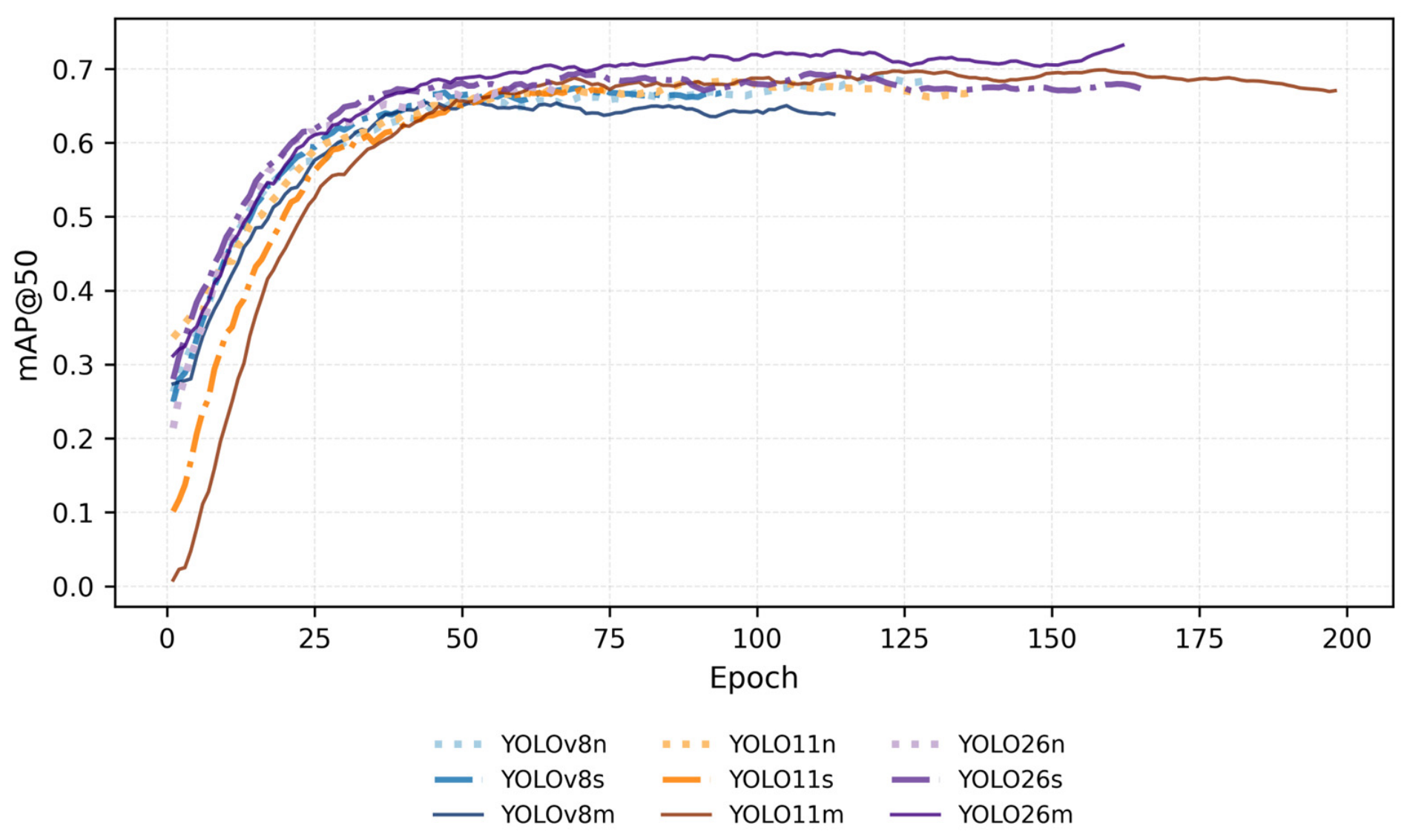
In Figure 8, the mAP evolution during training for three-class detection can be observed. In this case, YOLO26m and YOLO11m show a more favorable trend. However, the curves of all models exceed approximately 0.62, while the models with better trends remain close to 0.7. When comparing these values with Table 5, the mAP@50 results are higher than 0.772. This may be related to the oscillations during training, as the values go up and down between epochs. Therefore, the curve shows the general trend, but it does not always match the highest values reached or the final results reported in the table.
Figure 8.
Comparison of model performance in the multiclass detection task for Foxtail, evaluating the behavior of the mAP@50 metric.
Figure 9 presents the evolution of recall during training. Again, a more oscillatory trend can be observed, showing that recall remains a challenge for the models, especially in the three-class configuration where it has lower results. YOLO26m shows the most favorable trend, followed by YOLO26s and YOLO11m, while YOLOv8m presents the lowest performance. Although YOLO11m had a slower start, its performance improved throughout training, reaching competitive values. This differs slightly from the final results presented in Table 5, where YOLO26m achieved the highest average recall, followed by YOLO11m and YOLO26n. These differences show that the evolution observed during training does not necessarily match the order of the best average results.
Figure 9.
Comparison of model performance in the multiclass detection task for Foxtail, evaluating the behavior of the Recall metric.
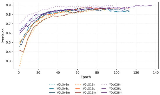
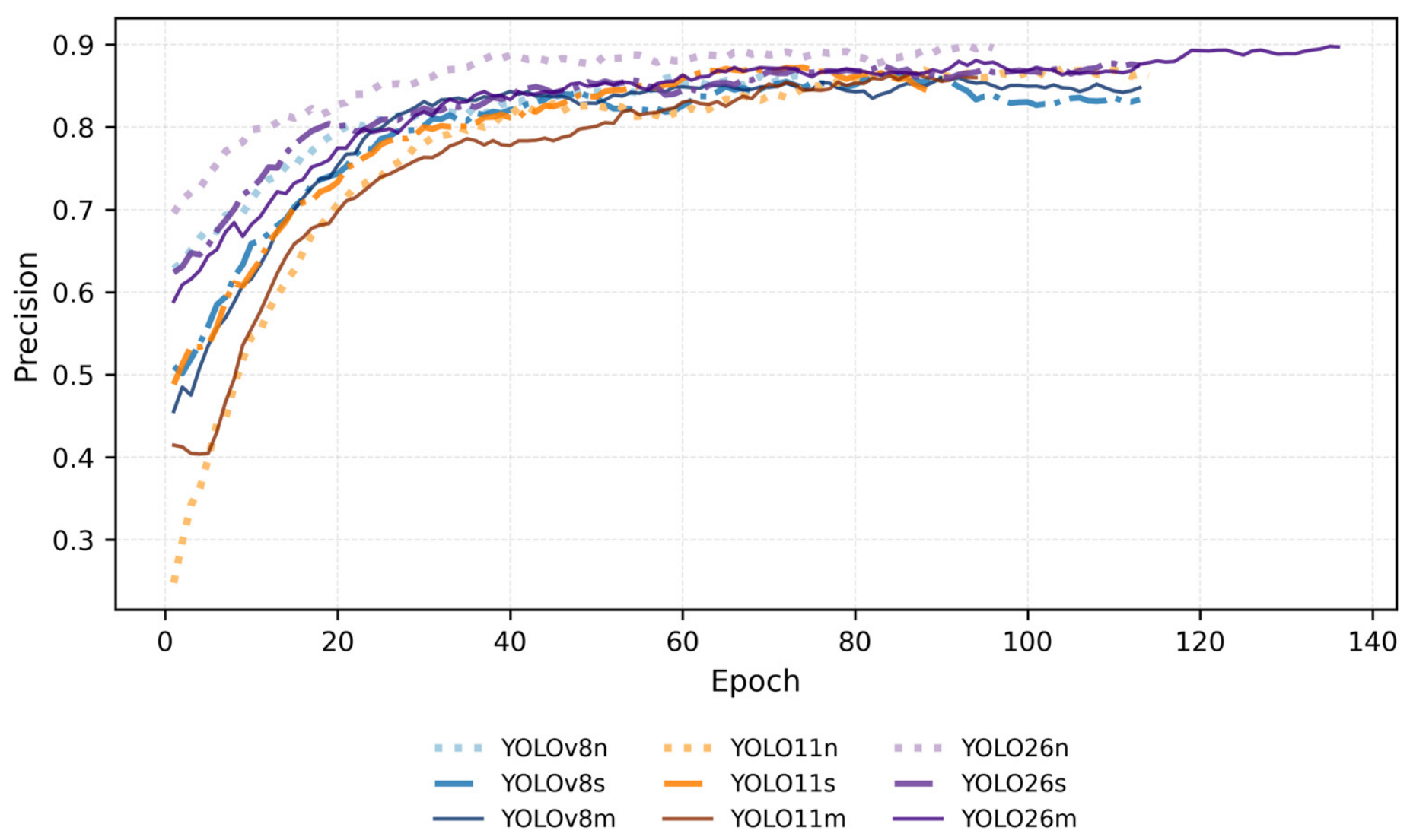
In the configuration presented in Figure 10, the precision achieved is lower compared to that presented in Figure 5. During training, this metric was one of those that showed the greatest variations, especially in the final epochs. Its values constantly fluctuated between values above and below the general trend, with these variations being even more pronounced than those observed in recall and mAP@50. This indicates that precision was one of the metrics that showed the greatest changes during each training epoch. Again, it was observed that YOLO11m had a slow start, but managed to improve its results as the epochs progressed, approaching the highest value recorded by YOLO26m. The highest values are reached by YOLO26m, YOLO11m, and YOLO26s, in that order, which is also related to the fact that these models had a longer training duration.
Figure 10.
Comparison of model performance in the multiclass detection task for Foxtail, evaluating the behavior of the Precision metric.
4. Discussion
As previously mentioned, no model consistently outperformed the others across all metrics. In this case, YOLO26s was selected for its ability to detect the plant, despite its moderate result in mAP@50-95, at stricter IoU confidence thresholds. Although YOLO26m also stands out, a lighter model was selected for this task to allow for higher FPS in a future real-time application.
For three-class detection, YOLO26m and YOLO26n stood out. In this case, YOLO26m was selected, whereas a lighter model was preferred for the previous configuration. Here, priority was given to a model with a better balance between precision and recall, a higher mAP@50–95, and a lower standard deviation. Therefore, YOLO26s with seed 41 and YOLO26m with seed 0 were selected as the models whose performance was closest to the mean of their respective configurations.
The model selected for single-class and three-class detection achieved an mAP@50 of 0.87 and 0.831 respectively. These results suggest that these models can identify the target foxtail classes in an acceptable manner, although with low performance compared to those found in other similar studies.
An example was the study [28], which reported mAP@50 values above 94%. However, this difference should not be interpreted solely because of the superiority of the models used, but rather as a direct consequence of the characteristics of the dataset. In this study, the authors began with a dataset containing labeling errors and inconsistent annotations, which were subsequently corrected, cleaned, and expanded, resulting in a significant improvement in model performance, with mAP@50 increasing from approximately 84% to more than 94%. This highlights the great influence that the dataset and label quality have on model training.
The size and composition of the dataset are important variables that should be considered. The primary dataset used in [28] was obtained from Kaggle and contained 1300 images, which were later increased to 6975 images through data augmentation. Although the original dataset was smaller than ours after data augmentation, the 1300 images corresponded to different original images, providing greater natural variability in the dataset rather than variability generated through augmentation techniques.
There are also significant differences in the acquisition of the images. The dataset they presented had less variability in camera distance, framing and background, which were later enriched by data augmentation techniques such as rotations, flips, brightness adjustments, noise addition, and mosaic augmentation. These strategies allowed for a controlled and artificial increase in the diversity of the training set.
In contrast, in this study, the images were obtained mainly from the iNaturalist platform and underwent a manual selection and labeling process. This dataset is characterized by a high diversity of backgrounds and environments, ranging from rural to urban environments. This heterogeneity brought a greater challenge when having to learn to generalize across noticeable variations in illumination, perspective, background, and scale.
Another relevant aspect is related to the composition of the images. Many of the available photographs contained plants occupying a considerable portion of the frame, in some cases covering more than 90% of the image. Although some of these examples were discarded during the selection process, others were retained to take advantage of data augmentation techniques such as mosaic and zoom out, with the purpose of generating a greater variety of scenarios during training. Despite this, this characteristic brings another inconvenience for the detection stage, since Foxtail, whose inflorescences generally extend considerably above the tiller. This causes the bounding boxes to cover extensive regions of the image, incorporating a large portion of the background within the box.
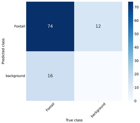
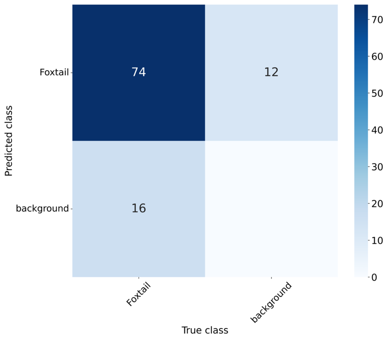
This can lead the model to associate environmental characteristics with the presence of the plant, making it more difficult to distinguish between the object of interest and the background. This behavior can be observed in the confusion matrix presented in Figure 11, where a significant portion of the errors associated with confusion with the background were recorded. In particular, the model correctly detected 74 Foxtails, while 16 were not detected and 12 were false detections that corresponded to the background. This suggests that the main difficulty corresponds to its inability to distinguish between the environment and the object of interest.
Figure 11.
Confusion matrix of the YOLO26s model for single-class detection on the test set.
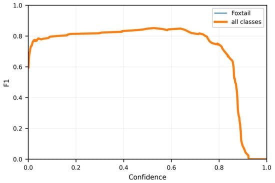
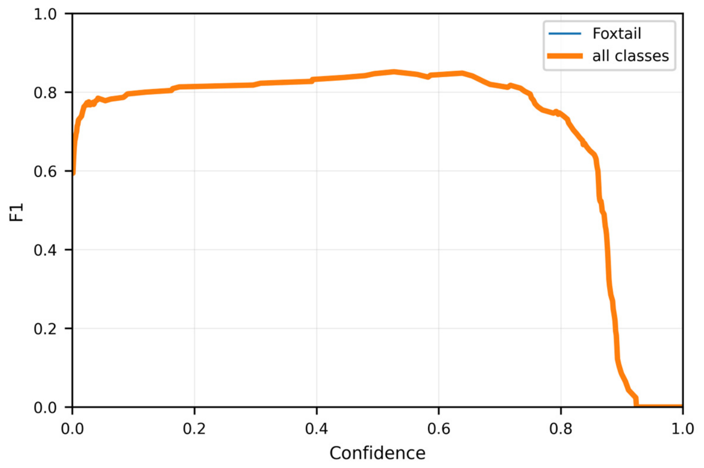
Figure 12 presents the F1-score curve, where a stable performance close to 0.8 can be observed up to a confidence level of approximately 0.75, followed by a more pronounced decrease from 0.8 onward. This indicates that the model maintains an acceptable balance between precision and recall across a broad confidence range before presenting a more marked decrease.
Figure 12.
F1-Confidence curve of the YOLO26s model for single-class detection on the test set.
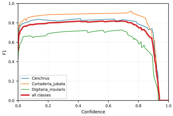
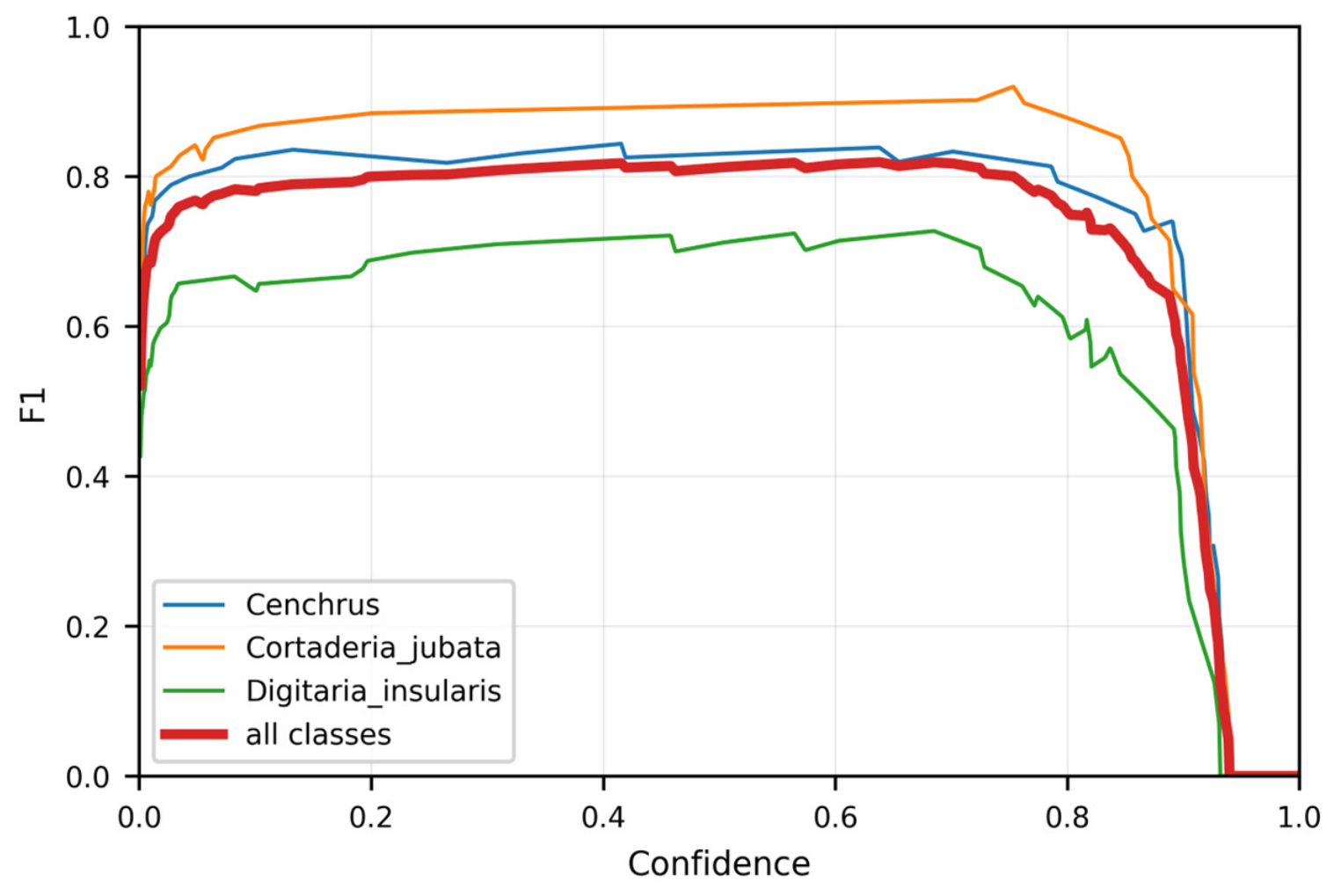
The three-class detection analysis allowed for a more detailed analysis of the previously mentioned results. Figure 13 shows the F1-score curve for each evaluated class, revealing differences in the model’s detection performance across classes. For most of the confidence range, Cortaderia jubata presented the best performance, followed by Cenchrus and, finally, Digitaria insularis. Although this order does not correspond to the one observed in Figure 3 in terms of the number of instances per class, Digitaria insularis had 462 fewer instances than Cortaderia jubata, which is a considerable difference that could have had a greater effect on its performance. However, to determine whether this lower performance is related to a greater number of cases being incorrectly identified as other classes, the confusion matrix can be analyzed.
Figure 13.
F1-Confidence curve of the YOLO26m model for three-class detection on the test set.
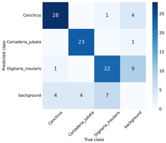
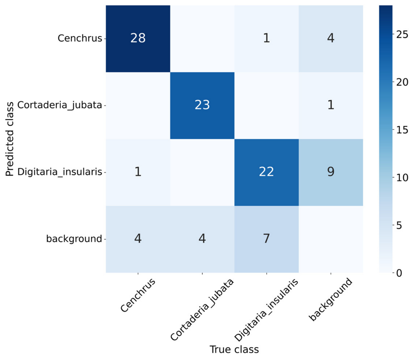
The confusion matrix (see Figure 14) confirmed that the main source of error is not confusion between classes, but confusion with the background. This was more common with the species Digitaria insularis, for which, out of 29 instances of this class, 7 were not detected by the model and one was detected as Cenchrus, making it the class that presents the greatest difficulty for the model to detect.
Figure 14.
Confusion matrix of the YOLO26m model for three-class detection on the test set.
As shown in the confusion matrix (Figure 14), the main factor contributing to the decrease in the evaluation metrics was not confusion between classes. Only one Cenchrus instance was detected as Digitaria Insularis, and one Digitaria insularis instance was detected as Cenchrus. Instead, the main difficulty was related to confusion between the plants and the surrounding environment. Most of the false positives corresponded to background detections, while the false negatives corresponded to plants that were not detected. Although Cenchrus had the highest number of correct detections, when comparing the proportion of correct detections relative to the total number of instances and predictions for each class, Cortaderia jubata presented the best performance, followed by Cenchrus and, finally, Digitaria insularis.
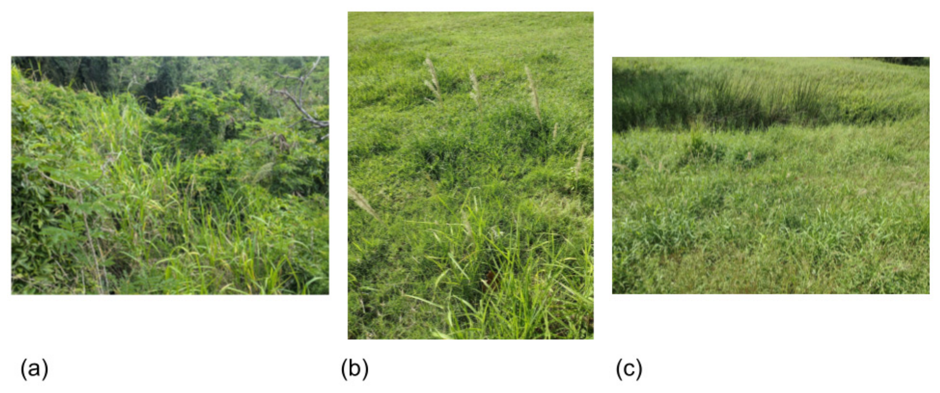
One possible reason for the poor Digitaria insularis performance might be the visual characteristics presented in the images of the class. In several cases, this species appears in environments dominated by vegetation, grasses, and rural areas, where the background presents morphology, color, and textures similar to those of the plant being identified. This increases the difficulty of visually distinguishing between the object and the environment, as shown in Figure 15.
Figure 15.
Examples of Digitaria insularis images present in the dataset. (a) [29] (b) [30] (c) [31].
Since this study evaluated the detection capability of the presented models without modifications, no additional filters or model modifications were applied to improve aspects such as detection capability or inference speed for weed detection, as has been explored in other studies. However, this could be considered in future work as a possible approach to improve the metrics and overall performance of the models.
When comparing the F1-score curves across confidence thresholds, similar performance was observed for single-class detection and three-class detection. Single-class detection reached a maximum F1-score of approximately 0.83 at a confidence threshold of 0.505, while three-class detection reached approximately 0.82 at a threshold of 0.655. This difference was minimal. It was also observed that three-class detection reached an F1-score close to 0.75 before a threshold of 0.1, whereas single-class detection reached a similar value after a threshold of 0.2. In addition, the F1-score for three-class detection remained close to 0.8 over a wider range of confidence thresholds.
The confusion matrices also showed similar results for both models. Single-class detection had 16 undetected instances and 12 incorrect detections associated with the background, compared with 15 undetected instances and 14 background-related incorrect detections for three-class detection.
The overall metrics obtained with Ultralytics for the selected models showed better results for single-class detection, with a precision of 0.911, recall of 0.800, mAP@50 of 0.852, and mAP@50-95 of 0.505. For three-class detection, the corresponding values were 0.878, 0.759, 0.810, and 0.501, respectively. Both configurations showed similar results at stricter IoU thresholds, while single-class detection achieved a slightly better result at mAP@50, suggesting a small difference in localization performance.
In the general comparison, the epoch-based curves showed better behavior for the models selected for single-class detection, presenting greater stability and better values for the evaluated metrics. Regarding inference speed, no clear advantage was found for either configuration. Although multiclass detection achieved higher FPS in most cases, this trend was not consistent across all models and depended on the measurement method used.
Furthermore, Table 7 presents the mean and standard deviation of each metric for all models in both configurations, allowing their performance to be compared. On average, single-class detection achieved higher values across the evaluated metrics, with differences close to 5% in most cases, while the difference for mAP@50–95 was approximately 2.8%, making it the metric with the lowest variation among the final results.
Table 7.
Comparison of the mean performance metrics (±standard deviation) obtained for the TCD and SCD configurations.
However, it is important to consider that even though both configurations are based on the same dataset, the augmentations applied were random, so the final datasets differed in their annotations. In addition, the same 5556 instances were distributed among three classes in the three-class configuration, while the single-class configuration contained the 5556 instances as a single class. This also favors the training of the single-class model, since it only needs to learn the characteristics and patterns associated with detecting a foxtail plant with respect to the background, rather than also distinguishing between three different classes. This behavior can also be observed in the F1-score, where the “all” value in the three-class configuration is affected by the lower performance obtained by some of the individual classes.
Although the detection capability of these architectures was evaluated using the iNaturalist-based dataset, the YOLO26 family generally presented competitive results. In several cases, its variants were among the highest-performing models for the different metrics, even occupying more than one of the first positions. However, for future work, it would be important to evaluate their performance in real-world and real-time scenarios, where the models can be tested with a dataset that differs from the conditions to which they were exposed during training.
If the current metrics were maintained in a real-world scenario, the selected model could potentially achieve adequate performance by detecting most of the foxtails present. However, the mAP@50-95 values indicate that the detections would not necessarily be as precise as expected in terms of localization, meaning that the model could identify the plant correctly but cover more or less of the actual plant with the bounding box. At the same time, the precision obtained could help reduce false detections. If the three-class approach were selected, more errors associated with the background could be expected, while only a small number of cases would involve confusion between classes. Therefore, this configuration could be considered when identifying the specific class or species group is required.
5. Conclusions
The obtained results highlight the importance of the dataset for the performance of object detection models. Factors such as class imbalance, annotation inconsistency, and variability in acquisition conditions can affect the model’s ability to correctly detect weeds and distinguish between classes. Furthermore, the characteristics of the plants evaluated can result in bounding boxes that include portions of the background, making it more difficult to distinguish the object from its surroundings. This was particularly evident in Digitaria insularis, where the visual similarity between the plant and its surrounding environment affected its detection performance.
The YOLO architectures demonstrated a good ability to classify between classes but relatively low performance in their localization. The main challenge was the omission of instances, mainly associated with the difficulty of finding the plants due to confusion with the background, especially with Digitaria insularis. In future works, the effect of including preprocessing or filtering techniques can be evaluated, including possible model modifications that favor the differentiation between the plant and the background present in the image in cases where both the instance and the environment have high visual similarity.
The YOLO26 family presented the most competitive overall performance among the evaluated architectures. YOLO26s stood out in the single-class configuration, while in the three-class configuration, no single model dominated all the evaluated metrics, although YOLO26 variants remained among the most competitive. YOLOv8 showed good inference speed, but it was not consistently the fastest architecture in all measurements. Overall, the results indicate that YOLO26 can provide a good balance between detection performance and inference speed, although the best variant depends on the detection configuration and the requirements of the application.
Overall, the results show that YOLO architectures can be used for the detection of the evaluated Foxtail species, achieving an acceptable performance under the conditions of the dataset used. However, the results also show that the detection performance is affected by the visual similarity between the plants and the environment, as well as the configuration used, whether single- or multiclass detection.
Author Contributions
Conceptualization, J.C., J.J. and E.I.G.-V.; methodology, J.C., J.J. and E.I.G.-V.; software, J.C., J.J. and E.I.G.-V.; validation, J.C., J.J. and E.I.G.-V.; formal analysis, J.C., J.J. and E.I.G.-V.; investigation, J.C., J.J. and E.I.G.-V.; resources, J.C., J.J. and E.I.G.-V.; data curation, J.J.; writing—original draft preparation, J.C., J.J. and E.I.G.-V.; writing—review and editing, J.C., J.J. and E.I.G.-V.; visualization, J.C., J.J. and E.I.G.-V.; supervision, J.C.; project administration, J.C. and E.I.G.-V.; funding acquisition, J.C. and E.I.G.-V. All authors have read and agreed to the published version of the manuscript.
Funding
This research received no external funding.
Institutional Review Board Statement
Not applicable.
Informed Consent Statement
Not applicable.
Data Availability Statement
The original contributions presented in this study are included in the article. The datasets used in this study are publicly available through Roboflow Universe (see Section 2.1). Further inquiries can be directed to the corresponding author.
Acknowledgments
We gratefully acknowledge the support of Universidad Militar Nueva Granada for providing access to its research infrastructure and institutional resources, which were instrumental in carrying out the work presented here.
Conflicts of Interest
The authors declare no conflicts of interest.
Abbreviations
The following abbreviations are used in this manuscript:
| CNN | Convolutional Neural Networks |
| SVM | Support Vector Machine |
| ANN | Artificial Neural Network |
| RCNN | Region-based Convolutional Neural Network |
| STAL | Small-Target-Aware Label Assignment |
| NMS | Non-Maximum Suppression |
| DFL | Distribution Focal Loss |
| AMP | Automatic Mixed Precision |
| CUDA | Compute Unified Device Architecture |
| YOLO | You Only Look Once |
| TP | True positive |
| FN | False Negative |
| IoU | Intersection over Union |
| Box Predicted | |
| Box Ground Truth | |
| AP | Average Precision |
| mAP | Mean Average Precision |
| Exponential Moving Average | |
| SD | Standard Deviation |
| TCD | Three-Class Detection |
| SCD | Single-Class Detection |
References
- Galon, L.; Balla, C.D.; Henz Neto, O.D.; Tedesco, L.; Concenço, G.; Franco, Â.M.P.; Ribeiro dos Anjos, A.D.; Dassoler, O.A.; Trezzi, M.M.; Perin, G.F. Morphophysiological and Nutritional Responses of Bean Cultivars in Competition with Digitaria insularis. Plants 2025, 14, 2684. [Google Scholar] [CrossRef] [Scilit]
- Tomazini, J.; Bittencourt, H.V.H.; Bonome, L.T.D.S.; Penha, L.A.O.; Passini, T. The population density of Digitaria insularis influences Phaseolus vulgaris agronomic traits. Res. Soc. Dev. 2022, 11, e18611628924. [Google Scholar] [CrossRef] [Scilit]
- Ministerio para la Transición Ecológica. Estrategia de Gestión, Control y Posible Erradicación del Plumero de la Pampa (Cortaderia selloana) y Otras Especies de Cortaderia; Ministerio para la Transición Ecológica: Madrid, Spain, 2018. Available online: https://www.miteco.gob.es/content/dam/miteco/es/biodiversidad/publicaciones/estrategias/estretegia_cortaderia_tcm30-478427.pdf (accessed on 5 June 2026).
- Comisión Nacional para el Conocimiento y Uso de la Biodiversidad. Método de Evaluación Rápida de Invasividad (MERI) para Especies Exóticas en México: Cortaderia selloana (Schult. & Schult. f.) Asch. & Graebn., 1900; Comisión Nacional para el Conocimiento y Uso de la Biodiversidad (CONABIO): México City, Mexico, 2016. Available online: https://www.gob.mx/cms/uploads/attachment/file/221000/Cortaderia_selloana.pdf (accessed on 5 June 2026).
- Global Invasive Species Database. Cortaderia jubata. [Online]. Available online: https://www.iucngisd.org/gisd/speciesname/Cortaderia+jubata (accessed on 27 September 2026).
- California Invasive Plant Council. Cortaderia jubata Profile. Available online: https://www.cal-ipc.org/plants/profile/cortaderia-jubata-profile/ (accessed on 27 September 2026).
- Miller, W.; Mann, J.J.; Buhl, K. Pasto Jubata y Pasto de la Pampa. Available online: https://solvepestproblems.oregonstate.edu/es/node/1586 (accessed on 27 September 2026).
- Raza, H.; Abu Bakr, M.; Khan, S.D.; Batool, H.; Ullah, H.; Ullah, M. Benchmarking YOLO Models for Crop Growth and Weed Detection in Cotton Fields. AgriEngineering 2025, 7, 375. [Google Scholar] [CrossRef] [Scilit]
- Lu, Z.; Zhu, C.; Liu, L.; Yang, Y.; Wang, J.; Xia, W. Star-YOLO: A lightweight and efficient model for weed detection in cotton fields using advanced YOLOv8 improvements. Comput. Electron. Agric. 2025, 235, 110306. [Google Scholar] [CrossRef] [Scilit]
- Al-Ahmadi, A.H.; Subr, A.K. Smart sprayer for weed control using an object detection algorithm (YOLOv5). J. Plant Prot. Res. 2025, 65, 311–323. [Google Scholar] [CrossRef] [Scilit]
- Liang, B.; Hu, L.; Liu, G.; Hu, P.; Xu, S.; Jie, B. YOLOv9-GSSA model for efficient soybean seedlings and weeds detection. Smart Agric. Technol. 2025, 12, 101134. [Google Scholar] [CrossRef] [Scilit]
- Dang, F.; Chen, D.; Lu, Y.; Li, Z. YOLOWeeds: A novel benchmark of YOLO object detectors for multi-class weed detection in cotton production systems. Comput. Electron. Agric. 2023, 205, 107655. [Google Scholar] [CrossRef] [Scilit]
- Jyostna, J.; Abhiram, K.; Abhishek, C.; Sharma, D.A. An Automated Weed-Detection Approach Using Deep Learning in Agriculture System. In Proceedings of the 2025 International Conference on Advanced Computing Technologies (ICoACT), Sivalasi, India, 14–15 March 2025; pp. 1–7. [Google Scholar] [CrossRef] [Scilit]
- Vikashini, G.; Arunkumar, S. Machine Learning Based Weed Detection in Zucchini farm. In Proceedings of the 2025 International Conference on Advances in Modern Age Technologies for Health and Engineering Science (AMATHE), Shivamogga, India, 24–25 April 2025; pp. 1–6. [Google Scholar] [CrossRef] [Scilit]
- Habib, M.; Sekhra, S.; Tannouche, A.; Ounejjar, Y. Enhancement of YOLOv5 for automatic weed detection through backbone optimization. IAES Int. J. Artif. Intell. 2025, 14, 658–666. [Google Scholar] [CrossRef] [Scilit]
- C. Amigon, cypamigon/inat_downloader. (26 de julio de 2026). Python. [Online]. Available online: https://github.com/cypamigon/inat_downloader (accessed on 28 July 2026).
- evan8, “Cenchrus alopecuroides,” iNaturalist, November 2016. Available online: https://www.inaturalist.org/observations/448359 (accessed on 30 September 2026).
- charlie, “Cenchrus setaceus,” iNaturalist, 4 July 2015. Available online: https://www.inaturalist.org/observations/172377 (accessed on 28 September 2026).
- al_kordesch, “Cortaderia jubata,” iNaturalist, 29 August 2022. Available online: https://www.inaturalist.org/observations/132898160 (accessed on 28 September 2026).
- kevinfaccenda, “Digitaria insularis,” iNaturalist, 4 March 2023. Available online: https://www.inaturalist.org/observations/150553832 (accessed on 28 September 2026).
- Ultralytics, Ultralytics YOLO26. Available online: https://docs.ultralytics.com/es/models/yolo26 (accessed on 10 February 2026).
- Hidayatullah, P.; Tubagus, R. YOLO26: A Comprehensive Architecture Overview and Key Improvements. arXiv 2026, arXiv:2602.14582. [Google Scholar] [CrossRef] [Scilit]
- Sharma, S.; Vardhan, M. Advancing Precision Agriculture: Enhanced Weed Detection Using the Optimized YOLOv8T Model. Arab. J. Sci. Eng. 2025, 50, 7343–7360. [Google Scholar] [CrossRef] [Scilit]
- Chen, Z.; Chen, B.; Huang, Y.; Zhou, Z. GE-YOLO for Weed Detection in Rice Paddy Fields. Appl. Sci. 2025, 15, 2823. [Google Scholar] [CrossRef] [Scilit]
- Ma, C.; Chi, G.; Ju, X.; Zhang, J.; Yan, C. YOLO-CWD: A Novel Model for Crop and Weed Detection Based on Improved YOLOv8. Crop Prot. 2025, 192, 107169. [Google Scholar] [CrossRef] [Scilit]
- Huang, J.; Xia, X.; Diao, Z.; Li, X.; Zhao, S.; Zhang, J.; Zhang, B.; Li, G. A Lightweight Model for Weed Detection Based on the Improved YOLOv8s Network in Maize Fields. Agronomy 2024, 14, 3062. [Google Scholar] [CrossRef] [Scilit]
- Arsyad, C.F.; Andono, P.N.; Soeleman, M.A. Hyperparameter Tuning with Optuna to Optimize the YOLOv11n Model for Weed Detection. J. RESTI Rekayasa Sist. Teknol. Inf. 2025, 9, 1153–1162. [Google Scholar] [CrossRef] [Scilit]
- Rahman, M.M.; Rahim, U.F. Real-Time Weed Detection Using Advanced Object Detection Models: A Comparative Study. In Proceedings of the 2025 2nd International Conference on Next-Generation Computing, IoT and Machine Learning (NCIM), Gazipur, Bangladesh, 27–28 June 2025; pp. 1–6. [Google Scholar] [CrossRef] [Scilit]
- Faccenda, K. Digitaria insularis, iNaturalist. 28 May 2025. Available online: https://www.inaturalist.org/observations/285530979 (accessed on 28 September 2026).
- Faccenda, K. Digitaria insularis, iNaturalist. 22 September 2022. Available online: https://www.inaturalist.org/observations/136515515 (accessed on 28 September 2026).
- Faccenda, K. Digitaria insularis, iNaturalist. 21 January 2023. Available online: https://www.inaturalist.org/observations/147316409 (accessed on 28 September 2026).

Disclaimer/Publisher’s Note: The statements, opinions and data contained in all publications are solely those of the individual author(s) and contributor(s) and not of MDPI and/or the editor(s). MDPI and/or the editor(s) disclaim responsibility for any injury to people or property resulting from any ideas, methods, instructions or products referred to in the content. |
© 2026 by the authors. Licensee MDPI, Basel, Switzerland. This article is an open access article distributed under the terms and conditions of the Creative Commons Attribution (CC BY) license.