


Abstract
The growing energy demand and dependence on hydroelectric systems due to climate change have increased the need for sustainable energy alternatives for rural and non-interconnected regions. Biodigesters represent a promising option for decentralized energy production from organic waste; however, their efficiency can be affected by environmental variables such as altitude and temperature, particularly in countries with mountainous geography such as Colombia. This study develops a physics-informed machine learning framework to estimate specific energy efficiency (kWh/kg) in biogas digestion systems. In this article, specific energy efficiency (SEE) is used as a mass-normalized measure of energy performance, taking into account the energy content of methane associated with specific biogas production, rather than as a conventional dimensionless thermodynamic efficiency. To start, a baseline Random Forest Regressor was trained using an empirical literature-based dataset (N = 103), and was then compared with an XGBoost model that incorporated physically derived variables, 400 synthetic observations generated using phenomenological relationships, and differential weighting of the samples. Performance was evaluated using repeated nested cross-validation with five partitions and five repetitions, with hyperparameter optimization performed via grid search exclusively within the internal training partitions, while keeping the empirical evaluation observations independent of the optimization process and the synthetic data. Random Forest achieved an average R2 of 0.1598 ± 0.0706, an MAE of 0.4703 ± 0.0222 kWh/kg, and an sMAPE of 35.76 ± 1.52%, while XGBoost achieved R2 = 0.2263 ± 0.1554, MAE = 0.4631 ± 0.0326 kWh/kg, and sMAPE = 37.87 ± 1.29%. Although the XGBoost model presented better point estimates for R2 and MAE, the results did not show statistically conclusive superiority. Furthermore, the ablation study showed that the components of the framework did not contribute equally; data augmentation with synthetic data yielded the most favorable results in terms of error reduction. Additionally, permutation importance analysis identified altitude, ambient temperature, operating temperature, and hydraulic retention time as the predictors with the most consistent contributions. Thus, these results support the use of physics-informed approaches as exploratory tools for modeling the performance of bioreactors under variable environmental conditions, while also highlighting the need to expand the experimental basis and conduct external validations before their widespread application.
1. Introduction
Today, the world faces a complex energy scenario characterized by persistent growth in electricity demand and the challenges of implementing truly sustainable solutions on a large scale. Colombia is not an exception to this challenge. Although its energy matrix has been historically based on hydropower generation [1], the effects of climatic and hydrological variability have significantly reduced reserve levels, threatening the energy supply of cities such as Bogotá. While alternative energy sources such as solar and wind have been promoted, particularly through projects located in La Guajira [2], their deployment has progressed more slowly than expected due to various social, technical, and infrastructure-related challenges. Taking this into account, it becomes necessary to explore complementary, decentralized and less directly dependent on the availability of water resources energy sources.
One of these alternatives is biogas produced through anaerobic digestion in biodigesters, a technology particularly attractive for rural and non-interconnected zones (NIZs), where agricultural activities generate organic waste with energy potential [3,4]. However, the performance of these systems is influenced not only by biodigester design or substrate type but also by environmental conditions such as altitude above sea level and ambient temperature. Colombia’s geography features wide altitudinal and thermal gradients, with settlements and agricultural and livestock activities distributed from low-altitude areas to Andean regions located several thousand meters above sea level. These conditions result in significant environmental heterogeneity among regions, particularly in terms of temperature and atmospheric pressure—variables that are potentially relevant to the biological and energetic processes associated with anaerobic digestion [5]. Studies conducted in countries such as Nepal and India have reported reductions of up to 40% in biogas production during winter due to decreased microbial activity under cold conditions [6].
International evidence shows that the performance of anaerobic digestion systems can be sensitive to environmental operating conditions. In high-altitude and cold-climate regions, reductions of up to 60% in methane production have been reported due to changes in the pH-temperature balance and reduced bacterial kinetics [6,7]. These effects are primarily associated with the anaerobic digestion stage. Furthermore, altitude can also independently influence the subsequent stage of biogas energy utilization, since lower air density and reduced oxygen availability at higher altitudes can affect combustion conditions and the performance of power generation systems based on internal combustion engines. Consequently, altitude and temperature conditions must be taken into account both in the analysis of the biogas production process and in the evaluation of its subsequent energy utilization [8].
In the electrical conversion stage, studies conducted with biogas-fueled engine-generator systems have reported electrical efficiencies ranging from 6% to 20.9%, depending on factors such as the stability of the biogas composition, air-fuel mixture conditions, and engine operating parameters [9]. This electrical efficiency specifically refers to the process of converting biogas into electricity and is conceptually different from the specific energy efficiency (SEE, kWh/kg) used as the target variable in this study. As summarized in Table 1, the available evidence shows that environmental and operational conditions can affect different stages of the biogas energy utilization chain, from anaerobic digestion to its final conversion into useful energy.
Table 1.
Summary of previous studies on the impact of environmental and operational variables on biodigester system efficiency.
Although these environmental and operational effects have been extensively studied in various contexts, there remains a gap in the development of estimation tools tailored to rural and decentralized biogas systems that integrate, within a single framework, environmental variables such as altitude and temperature with biogas digester operational and design parameters. This need is particularly relevant in contexts with high topographic heterogeneity, such as Colombia, where the availability of detailed experimental data and continuous instrumentation may be limited. In this regard, approaches are needed that can estimate energy performance indicators based on a limited set of available variables, without necessarily relying on exhaustive biochemical characterization or continuous monitoring systems.
The field of anaerobic digestion modeling has evolved through various approaches, among which the Anaerobic Digestion Model No. 1 (ADM1) stands out, as it allows for a highly detailed representation of the biochemical processes involved in the degradation of organic matter. However, their implementation requires a considerable number of state variables, kinetic parameters, and calibration processes, which can limit their application when available information is scarce or comes from rural systems that lack sufficient instrumentation [12].
Different modeling strategies have been applied to anaerobic digestion and related bioenergy processes. Mechanistic approaches such as ADM1 provide a detailed representation of biological and physicochemical transformations, but require extensive parameterization and process information that may not be consistently available in data-limited applications. Data-driven machine-learning models offer greater flexibility for capturing nonlinear relationships and have been applied to biogas prediction, monitoring, and process optimization; however, their performance remains dependent on data quality, dataset size, and the representativeness of the conditions used for training. More recently, physics-informed and hybrid approaches have sought to combine data-driven prediction with prior process knowledge, either by incorporating physical constraints into the learning process or by using mechanistic models to generate auxiliary training information. Table 2 summarizes these modeling approaches and clarifies how the framework developed in this study differs in objective, data requirements, and validation scope.
Table 2.
Comparison of representative modeling approaches for anaerobic digestion and related bioenergy processes and their relationship to the present study.
These limitations make it difficult to plan bioenergy systems in rural and cold-climate regions, where detailed experimental data are typically scarce. Due to the lack of estimation tools that jointly account for environmental conditions and the main operational parameters of the biodigester—without requiring specialized equipment—it is challenging to predict how its energy performance may vary across sites with different topographic and thermal characteristics. Furthermore, when performance falls short of expectations, the interplay of environmental, operational, and design factors makes it difficult to attribute such variations to a single variable. For this reason, having estimation tools that integrate these variables can aid in the preliminary sizing of biogas systems, without replacing a detailed technical assessment of each facility.
This study develops and evaluates a machine learning framework to estimate the specific energy efficiency (SEE, kWh/kg) of biogas systems under different environmental and operational conditions. In this work, the SEE is used as an energy performance indicator normalized by mass, rather than as a conventional dimensionless thermodynamic efficiency; its definition and calculation are formally presented in Section 2.3.
The problem is addressed from an empirical perspective using a Random Forest model, and the XGBoost-based framework incorporates physical information through derived variables and a data augmentation strategy based on phenomenological relationships associated with temperature and altitude. In this way, the study compares a reference model based exclusively on empirical observations with a physics-informed approach, and separately evaluates the contribution of its main components to estimation performance.
The main contributions of this research are the following:
- Comparative evaluation under a robust validation scheme: A Random Forest model based solely on empirical observations is established as a reference and compared with the XGBoost-based framework using repeated nested cross-validation. This process allows us to evaluate estimation performance without using external test observations during hyperparameter selection and to quantify the variability of results across different data partitions. Furthermore, validation across independent studies allows us to examine how heterogeneity among experimental sources affects the models’ generalization ability.
- Integration of physical information through synthetic data augmentation and derived variables: A physics-informed data augmentation strategy is developed that incorporates phenomenological relationships associated with the thermal dependence of the process and with the effect of altitude on atmospheric pressure. Based on these relationships, synthetic observations are generated, and derived variables intended exclusively for training are incorporated. The aim is not to exactly reproduce the joint distribution of the empirical data, but rather to introduce explicit physical trends that can complement a limited and heterogeneous dataset.
- Evaluation of the individual contribution of the components and interpretation of the model: Through an ablation study, the effect of derived physical variables, the augmentation with synthetic data, and the differential weighting of observations are analyzed separately, avoiding the joint attribution of performance variations to the entire framework. In addition, permutation-based importance analysis on out-of-sample observations allows us to identify which variables maintain a more consistent estimative contribution and to differentiate between the internal importance assigned by XGBoost and the incremental information actually provided during evaluation.
The rest of the article is organized as follows. Section 2 presents the materials and methods, including the conceptual modeling of the system, database construction and preparation, definition of specific energy efficiency (SEE), a physics-informed data augmentation strategy, machine learning architectures, and the training and validation scheme used to evaluate their performance and robustness. Section 3 presents the results of the comparative analysis between Random Forest and XGBoost, along with evaluations of statistical robustness, generalization across studies, representativeness of the synthetic data, ablation of framework components, and model interpretability. Section 4 discusses the findings, their implications for modeling biodigestion systems under heterogeneous environmental conditions, and the main limitations of the study. Finally, Section 5 summarizes the conclusions and outlines the main areas for future research.
2. Materials and Methods
2.1. Conceptual System Modeling
The methodological framework of the study is based on conceptual modeling as a tool for defining the system, identifying relevant variables, and establishing the relationships that are subsequently represented by machine learning models. Taking into account the systems analysis approach proposed by Grant and Swannack [12], the specific energy performance associated with biogas production in the biodigester was defined as the object of study. Consequently, the subsequent stage of biogas conversion via an engine–generator system is not part of the target variable estimated by the models and is considered solely as a possible subsequent stage of energy utilization.
Based on the information available in the compiled studies, five empirical variables were selected as the main inputs: elevation above sea level, ambient temperature, biodigester operating temperature, biodigester volume, and hydraulic retention time (HRT). These variables were used by the reference Random Forest model. Meanwhile, for the physics-based framework, two additional derived variables were included: atmospheric pressure, calculated from altitude using a hypsometric relationship, and a heat loss index defined based on the biodigester volume. It is worth noting that these derived variables do not correspond to additional measurements but rather to deterministic transformations of already available variables. The variables, units, origin, and use in each modeling approach are summarized in Table 3.
Table 3.
Variables used in the empirical and physics-informed machine-learning frameworks.
Temperature and altitude-related conditions were taken into account due to their relationship with the physical and biological processes that influence anaerobic digestion. However, internal variables such as microbial activity or reaction kinetic constants were not measured directly on an empirical basis; their behavior was incorporated only indirectly during the generation of synthetic data informed by phenomenological relationships, as described later in Section 2.4.
The output variable for both models is specific energy efficiency (SEE, kWh/kg), defined in this study as an energy indicator normalized by mass and formally described in Section 2.3. Figure 1 below shows the conceptual flow of the two evaluated models: (a) a reference empirical model based on Random Forest and five observed variables; and (b) an XGBoost-based framework that complements the empirical variables with derived variables and physics-informed data augmentation.
Figure 1.
Conceptual information-flow architecture of the proposed estimation model: (a) Baseline Random Forest Model based on empirical records; (b) phenomenological XGBoost model incorporating hybrid data increase and physical laws.
2.2. Database Construction and Variable Definition
The empirical database was constructed using information reported in scientific studies on anaerobic digestion systems operated under different environmental and design conditions. The initial dataset consisted of 103 records. For each observation, the following variables were considered, when available: elevation above sea level, ambient temperature, biodigester operating temperature, reactor volume, hydraulic retention time (HRT), specific biogas yield, and methane content. The first five variables correspond to the empirical variables used by the models, while biogas yield and methane content were subsequently used to calculate the objective variable defined in Section 2.3.
Initially, a completeness check was performed on the required variables. Records with missing information in any of the variables necessary to construct the model inputs or calculate the target variable were excluded from the initial set of records, without imputing missing values. Of the 103 original records, 98 met the completeness criteria and formed the empirical basis used during the modeling process. The 103 original records are included in Appendix A, Table A1, to ensure traceability of the data extraction and to explicitly identify the cases excluded from the analysis.
Because the information was compiled from multiple studies, each observation was assigned a study identifier (Study_ID) corresponding to its source. This identifier was incorporated to enable a subsequent specific assessment of generalizability to studies not used during training. The original dataset comprised 12 study groups, of which 10 remained after applying the completeness criterion.
The compiled records show a wide range in the scale of the reported systems, with volumes ranging from 0.00052 m3 to 930 m3. The minimum value corresponds to an experimental reactor reported in one of the sources included in the compilation; it was retained because it represents a complete empirical observation, and no exclusion criterion based solely on reactor volume had been previously established. Excluding this record at a later stage solely based on its scale would have introduced an additional selection criterion that was not defined during the construction of the database. However, its inclusion does not imply that very small-scale reactors are directly representative of rural biodigesters at the implementation scale. On the contrary, the wide range of volumes demonstrates the heterogeneity of the compiled studies and is recognized as a limitation when extrapolating model results across systems of vastly different scales.
Finally, of the 98 complete records, 75 fall within the predefined operational range used for the predictive performance evaluation (0.3–3.5 kWh/kg). This criterion was applied only during the model evaluation and not as a preliminary filter for the records available for training. The definition and application of this domain are described in greater detail in Section 2.6. Table 4 presents the descriptive statistics of the original empirical dataset.
Table 4.
Descriptive statistics of the empirical database extracted from the literature review (N = 103).
2.3. Definition of Specific Energy Efficiency
The target variable used in the models was defined as specific energy efficiency (SEE), expressed in kWh/kg. This indicator represents the energy content associated with the methane fraction present in the specific biogas production reported for each biodigestion system. Its calculation takes into account the specific biogas yield, the volumetric methane content, and the lower heating value of methane, according to Equation (1)
where Vbiogas corresponds to the specific biogas yield expressed in m3/kg, is the volumetric fraction of methane expressed as a decimal y, and LHV corresponds to the lower heating value of methane, set at 9.97 kWh/m3.
In this article, the term “specific energy efficiency” is used as a normalized energy performance indicator per unit of mass, rather than as a conventional dimensionless thermodynamic efficiency. Thus, the SEE does not represent a ratio of useful energy obtained to total energy supplied to the system, but rather the specific energy content associated with the methane potentially available from the produced biogas. With this in mind, it is possible to use a common metric in kWh/kg to compare the collected data and establish a single target variable for machine learning models.
It is also worth noting that the SEE does not account for the electrical conversion efficiency of a motor-generator or the losses associated with the subsequent conversion of biogas into electricity. Consequently, any analysis of electromechanical conversion is considered a subsequent and independent step from the objective variable modeled in this study.
2.4. Physics-Informed Synthetic Data Generation
Due to the limited number of available empirical observations, a data augmentation strategy was implemented for the XGBoost-based framework by generating 400 synthetic observations. It is worth noting that these observations do not replace the empirical records nor are they intended to replicate additional experiments; their sole purpose is to supplement the training set using phenomenological relationships that represent expected trends among altitude, temperature, atmospheric pressure, and the process’s thermal response. The number of synthetic observations was kept fixed at 400 throughout the analysis and was not subsequently adjusted based on the performance obtained on the validation sets. To ensure reproducibility, the data generator used a fixed random seed of 42.
The data generation process began with altitude h, sampled from a uniform distribution between 0 and 4200 m above sea level. Based on this variable, ambient temperature Ta was generated using a decreasing relationship with altitude, incorporating a random term to represent thermal variability between sites. This relationship is shown in Equation (2)
where εa ~ N(0, 22) and the clip function restricts the values to the specified interval. The volume of the bioreactor, V, was plotted on a logarithmic scale using the following Equation (3):
Ta = clip (30 − 0.0062h + εa, 5, 35)
V = 10u, u~U(−1, 3)
Corresponding to a range of 0.1 to 1000 m3. This range was defined to represent various operating scales without reproducing the extreme experimental value of 0.00052 m3 present in the empirical database.
The hydraulic retention time was calculated based on a random component and an altitude-dependent adjustment, as shown in Equation (4):
Next, the difference between the biodigester’s operating temperature and the ambient temperature was represented by a volume-dependent relationship, accompanied by a term for random variability, as shown in Equations (5) and (6):
ΔT = clip[2 log10(V) + εT, 0, 8], εT~N(0, 12)
Top = Ta + ΔT
As for atmospheric pressure P, it was calculated directly from altitude using the barometric relationship, as shown in Equation (7)
where P is expressed in kPa. Based on this variable, a relative pressure factor was also defined, as shown in Equation (8):
The temperature dependence of the process was incorporated using an Arrhenius expression applied to the operating temperature in Kelvin, as shown in Equation (9):
Using A = 1 × 10⁸, Ea = 50,000 J/mol, R = 8.314 J/(mol ∗ K) y T = Top + 273.15.
In the data generator, this kinetic response was normalized relative to the maximum value obtained within the synthetic dataset; therefore, the Arrhenius term was used to represent a relative thermal response rather than as an experimental estimate of an absolute kinetic constant.
To introduce an additional dependence on the scale of the biodigester, the factor used in Equation (10), shown below, was employed.
fv = 1 + 0.1 log10(V)
Thus, the synthetic reference SEE was then constructed by combining the normalized thermal response, the volume factor, and the relative pressure factor, as shown in Equation (11):
Finally, a random term εSEE~N(0, 0.152) was added to avoid a completely deterministic relationship between the inputs and the objective variable, and the synthetic response was restricted to the interval 0.05–4.5 kWh/kg, as shown in Equation (12):
SEEsyn = clip(SEEbase + εSEE, 0.05, 4.5)
For each synthetic observation, we also calculated the atmospheric pressure derived from altitude and the volume-based heat loss index, defined as HLI = 1/V. The latter was used as a derived geometric proxy rather than as a direct measurement of heat transfer. Consequently, the final synthetic dataset contains the same seven predictor variables used by the XGBoost framework and a synthetic SEE generated using the above relationships.
As mentioned earlier, the data generation strategy was designed to impose explicit physical trends and expand the range of conditions available during training, but not to exactly reproduce the joint distribution of the empirical dataset. For this reason, the similarity between the two datasets was subsequently evaluated using univariate and multivariate analyses of distribution, correlation structure, principal component analysis, and proximity in the feature space.
The results of these verifications are presented in Section 3. Furthermore, the synthetic observations were used exclusively during the training of configurations that included data augmentation and were never part of the empirical datasets used to calculate the evaluation metrics.
The full sequence used to construct the synthetic observations is summarized in Table 5 and schematically illustrated in Figure 2.
Table 5.
Sequential procedure used to generate the physics-informed synthetic observations employed for XGBoost training.
Figure 2.
Workflow used to generate the physics-informed synthetic observations.
2.5. Machine Learning Architectures
The computational implementation was structured around two machine learning approaches with distinct roles in the study, as conceptually summarized in Figure 1. The first is a Random Forest model used as an empirical benchmark, while the second is a framework based on Extreme Gradient Boosting (XGBoost) that incorporates physical information through the derived variables and data augmentation described in Section 2.1 and Section 2.4. Both models were formulated as regression problems and used specific energy efficiency (SEE, kWh/kg) as the target variable.
As for the first Random Forest approach, it was trained exclusively on empirical observations and used five estimated variables obtained directly from the compiled studies: altitude, ambient temperature, biodigester operating temperature, biodigester volume, and hydraulic retention time (HRT). This model was used as a reference to establish the achievable performance based on the observed variables, without incorporating synthetic data or the two additional physical transformations. Its use as a baseline allows for a comparison with the expanded framework without a priori attributing an advantage to either of the two modeling strategies.
The second approach was implemented using XGBoost and utilized seven predictive variables: the five empirical variables mentioned above, atmospheric pressure derived from altitude, and the heat loss index derived from volume (HLI), formally defined in Section 2.4. In the configurations that incorporated data augmentation, the 400 synthetic observations generated according to the procedure described in Section 2.4 were added only to the available empirical observations for training.
In the proposed configuration for the XGBoost framework, differential weighting was also applied to the training observations. Each empirical record was assigned a weight of 10, and each synthetic record a weight of 1, in accordance with Equation (13):
This weighting corresponds to sample weights and not to weights assigned to the estimator variables. Its purpose within the original framework was to give greater relative influence to the empirical evidence during model fitting, given that the synthetic observations outnumbered the actual observations available in each training set. The effective contribution of this weighting strategy, as well as that of the derived variables and synthetic augmentation, was subsequently evaluated through the ablation study described in Section 2.8.
No normalization or standardization procedures were applied to the variables prior to training. Furthermore, the derived variables were calculated deterministically for each individual observation and did not require the estimation of means, standard deviations, or other parameters from the entire dataset. The selection of hyperparameters and the strict separation between training, internal validation, and external evaluation are described separately in Section 2.6.
2.6. Training Strategy and Repeated Nested Cross-Validation
Nested validation was divided into two levels. At the external level, intended exclusively to evaluate the model’s generalization ability, the 98 empirical observations were divided using five-fold cross-validation. This procedure was repeated five times with different reproducible partitions (5 × 5), generating 25 combinations of training and external testing. Within each external training set, a second level of cross-validation was subsequently performed, used exclusively for hyperparameter selection.
In each of the 25 external iterations, the external test set was kept completely isolated during model development. Hyperparameter selection was performed using only the observations from the external training set through a three-fold internal cross-validation. Thus, no observations from the external test set influenced hyperparameter selection, the tuning of derived variables, or any other training decisions. Once the appropriate configuration was selected within the internal cycle, the model was retuned using the external training set and then evaluated a single time on its external test set.
For Random Forest, both the internal training and the final tuning of each iteration used only empirical observations. In the XGBoost framework, the synthetic observations described in Section 2.4 were incorporated only into the subsets designated for training. During internal optimization, each validation set consisted exclusively of empirical observations, while synthetic data were added only to the subset used to tune the model. Once the hyperparameters were selected, the external model was trained using the empirical observations available in the external training set plus the 400 synthetic observations. In the full configuration, the 10:1 sample weighting defined in Equation (13) was also applied at this stage. In no case were synthetic records incorporated into the internal validation or external test sets.
The XGBoost optimization evaluated the combinations of n_estimators, max_depth, learning_rate, and subsample listed in Table 6. The search space consisted of n_estimators = {100, 150, 200, 250, 300}, max_depth = {1, 2, 3, 4, 5, 6}, learning_rate = {0.01, 0.05, 0.10}, and subsample = {0.8, 1.0}. Table 6 also presents the search space used for Random Forest.
Table 6.
Hyperparameter search spaces used in the inner cross-validation procedure.
The external partitions were generated before applying the criterion associated with the operational evaluation domain. For this reason, all 98 complete observations remained available for the construction of the training and test sets, while the reported metrics were calculated only for the empirical observations in the external test set whose SEE fell within the predefined range of 0.3 to 3.5 kWh/kg. This interval was used as the operational evaluation domain and not as a criterion for declaring the remaining observations to be physically invalid or necessarily corresponding to measurement errors. The same criterion was consistently applied to both models and to all external partitions.
As a result of the repeated-measure design, each of the 75 empirical observations within the operational domain received a strictly out-of-sample prediction once in each complete repetition. Thus, at the end of the five repetitions, five out-of-fold (OOF) predictions were available for each evaluable record. These predictions were retained to calculate performance per repetition and for the supplementary statistical analyses described in Section 2.10.
This approach prevents the information contained in the observations used for external evaluation from influencing hyperparameter selection and maintains an explicit separation between the empirical records used for validation and the synthetic observations used for training.
The complete validation strategy is summarized in Figure 3. Panel (a) illustrates the repeated nested cross-validation procedure used for model development and performance evaluation, including the strict separation between training, internal validation, and external testing, whereas panel (b) presents the complementary Leave-One-Study-Out (LOSO) framework used to assess generalization across independent study sources.
Figure 3.
Validation framework combining repeated nested cross-validation and LOSO evaluation.
2.7. Assessment of Generalizability Across Studies
In addition to the validation procedure described above, a complementary evaluation was conducted to determine the models’ generalizability to experimental sources not used during training. This evaluation was necessary because the empirical observations collected come from different studies and, therefore, may share specific characteristics associated with experimental design, operating conditions, or data source. To preserve this structure, each record was associated with the study identifier (Study_ID) defined during the construction of the database.
A Leave-One-Study-Out (LOSO) scheme was used, in which all observations from a single study were simultaneously set aside as an external test set, while the records from the other studies were used to develop the model. This procedure was repeated successively until each of the studies represented in the full dataset had been excluded from training. In this way, no observations from the study under evaluation were used in model fitting or in the selection of its hyperparameters.
Hyperparameter selection was also kept separate from the external test set. Within each LOSO iteration, optimization was performed exclusively using the studies available in the external training set through a three-fold internal cross-validation also based on groups (GroupKFold). At this level, all observations belonging to the same Study_ID remained together in a single partition, preventing records derived from the same source from appearing simultaneously in the internal training and validation subsets. The same hyperparameter search spaces defined in Section 2.6 were used.
As in the main evaluation, the operational domain of 0.3–3.5 kWh/kg was applied only when calculating metrics based on observations from the reserved study. Therefore, a study could be included as a training set even if some of its observations fell outside that range. When an excluded study contained no observations within the operational domain, that iteration did not contribute to the calculation of performance metrics. Of the 10 study groups represented after the completeness criterion, nine contributed at least one observation within the evaluation domain, collectively comprising the 75 evaluable observations described previously.
The predictions obtained for each excluded study were retained as out-of-sample predictions and subsequently combined to calculate global generalization metrics. Because the number of observations varies considerably across studies, two complementary methods were used to summarize performance. First, global metrics were calculated based on the entire set of LOSO predictions, so that each observation was given equal weight. Second, for MAE and sMAPE, averages were calculated per study and then averaged across studies, thereby giving each experimental source equal influence regardless of its size. This second evaluation helped reduce the dominance of studies with a larger number of records when interpreting performance across sources.
The coefficient of determination R2 for each study was calculated only when the reserved group contained a sufficient number of observations to define it. For studies represented by a single evaluable observation, R2 was not reported, although MAE and sMAPE could still be calculated. Finally, LOSO predictions were used in the uncertainty analysis and in comparisons between models via resampling by study group, as described in Section 2.10.
2.8. Ablation Study Design
In order to independently evaluate the contribution of the main components incorporated into the XGBoost framework, an ablation study consisting of six controlled configurations (A0–A5) was designed. Unlike the comparison between Random Forest and XGBoost, this analysis kept the XGBoost architecture fixed across all configurations and modified only three elements of the framework: the inclusion of the two derived physical variables, the use of the 400 synthetic observations, and the differential weighting between empirical and synthetic records. In this way, the differences observed between configurations can be interpreted in terms of the components added or removed, without simultaneously introducing a change in the algorithm. The evaluated configurations are summarized in Table 7.
Table 7.
Configurations evaluated in the XGBoost ablation study.
Configuration A0 was defined as the internal reference for ablation and used only the five empirical variables: altitude, ambient temperature, operating temperature, biodigester volume, and HRT, without any synthetic data or derived variables. A1 maintained exclusively empirical training but incorporated atmospheric pressure and the volume-derived index.
Configurations A2 and A3 incorporated the 400 synthetic observations while retaining only the five empirical variables. In A2, the empirical and synthetic records were given equal training weights (1:1), whereas in A3, the 10:1 differential weighting described in Equation (13) was applied. This comparison allowed us to examine the effect of weighting when synthetic expansion was present, without simultaneously introducing the derived physical variables.
Finally, A4 and A5 used the seven predictor variables and the 400 synthetic observations. A4 assigned equal weight to empirical and synthetic records (1:1), while A5 incorporated the 10:1 weighting. A5 corresponds to the complete configuration proposed for the XGBoost framework, as it combines derived variables, synthetic expansion, and differential weighting. The inclusion of A4 made it possible to specifically evaluate whether the weighting provided additional improvement once the other components of the framework had been incorporated.
All configurations were evaluated using exactly the same external and internal partitions described in Section 2.6. The same repeated nested cross-validation scheme with five partitions and five repetitions was used, as well as the same XGBoost hyperparameter search space.
The evaluation operational domain of 0.3–3.5 kWh/kg was applied identically to all six configurations when calculating metrics on out-of-sample predictions. Furthermore, each evaluable record received an out-of-sample prediction in each of the five replicates, allowing for a comparison of the configurations on exactly the same observations. This paired design reduced the influence that differences in data partitions might have on the comparison of the components.
Based on these six configurations, paired comparisons were defined to examine four main questions: (i) whether the derived physical variables provide additional predictive information compared to the empirical variables; (ii) does augmenting the data with synthetic data alter predictive performance; (iii) does differential weighting provide an additional advantage when synthetic data are present; and (iv) does the full configuration A5 exhibit behavior distinct from the empirical baseline A0. The uncertainty associated with these comparisons was assessed using the resampling procedures described in Section 2.10.
2.9. Model Interpretability
Interpretability was evaluated using the full A5 configuration of the XGBoost framework, based on the 25 external models obtained through the repeated nested cross-validation described in Section 2.6. For each model, the hyperparameters previously selected within its corresponding internal validation cycle were retained, without performing a new optimization for interpretability purposes.
Two complementary approaches were used. First, XGBoost’s native gain-based importance was calculated and normalized within each model to obtain a comparable relative importance across the 25 external evaluations. The results were summarized using the mean, standard deviation, and stability of each variable’s ranking. This measure describes XGBoost’s internal use of the predictors but does not, on its own, represent their predictive contribution out-of-sample.
For this reason, a permutation importance analysis was additionally performed on the empirical observations of each external test set. For each predictor, 50 random permutations were performed while keeping the other variables unchanged, and its importance was defined as the increase in the MSE relative to the model’s original performance
where positive values indicate a deterioration in performance when the variable’s information is altered. The 50 permutations for each model were first averaged to obtain a single estimate per predictor and external model. Subsequently, the results from the five outer folds of each repetition were combined using a weighted average based on the number of observations evaluated, yielding one estimate per variable for each of the five complete repetitions. The final importance was summarized using the mean, standard deviation, and a 95% uncertainty interval at the repetition level.
Due to the deterministic relationship between altitude and atmospheric pressure, and between volume and the HLI index, a grouped permutation of the altitude–pressure and volume–HLI pairs was also performed. In each case, the same permutation was applied to both variables to preserve their internal relationship while breaking their association with the target variable. In this way, the analysis distinguished between XGBoost’s internal use of the variables (gain) and their predictive contribution out-of-sample (permutation importance). The results are presented in Section 3.
2.10. Statistical Analysis and Performance Metrics
All processing, training, and evaluation procedures were implemented in Python 3.12 using Scikit-learn 1.6.1, XGBoost 3.4.1, Pandas 2.2.2, and NumPy 2.1.3. Model performance was evaluated using the coefficient of determination (R2), the mean absolute error (MAE), and the symmetric mean absolute percentage error (sMAPE).
where yi corresponds to the observed SEE, to the model estimate, to the mean of the observed values, and n to the number of records evaluated. The MAE was reported in kWh/kg, while the sMAPE was used as a complementary relative measure due to the presence of SEE values close to zero, for which the conventional MAPE may exhibit high sensitivity.
Regarding repeated nested cross-validation, the metrics were calculated independently for each of the five complete repetitions and summarized using the mean and standard deviation. Additionally, since each of the 75 evaluable observations received five out-of-sample predictions, an aggregated OOF prediction was calculated for each record by averaging its five estimates. The metrics calculated on these aggregated predictions were reported as a supplementary analysis and distinguished from the averages obtained across replicates.
The uncertainty of the aggregated OOF metrics and of the paired differences between Random Forest and XGBoost was estimated using bootstrap resampling with 10,000 resamples of the observations and a random seed of 42, using the 2.5th and 97.5th percentiles as the limits of the 95% interval. As an additional comparison, the absolute errors of both models on the same records were compared using a two-sided signed Wilcoxon rank-sum test, with α = 0.05.
For the Leave-One-Study-Out analysis, uncertainty was further assessed using bootstrapping by study group: Study_IDs were resampled with replacement while retaining all observations belonging to each study. The same principle of paired comparison was applied to the contrasts defined in the ablation study, using both record-level resampling and resampling grouped by Study_ID. The results of these comparisons were interpreted based on the magnitude of the differences and their uncertainty intervals, avoiding the attribution of superiority between configurations when those intervals included the value zero.
3. Results
3.1. Empirical Dataset Characterization
The initial literature review consisted of 103 observations from 12 study groups. After applying the completeness criterion described in Section 2.2, 98 records from 10 studies retained all the variables required for modeling. Of these, 75 observations, corresponding to nine studies, fell within the operational evaluation range of 0.3–3.5 kWh/kg and were used to calculate the predictive metrics.
The distribution of observations across studies was uneven. In particular, studies E03 and E05 together accounted for 59 of the 75 evaluable records (78.7%), while other studies were represented by a considerably smaller number of observations. This structure indicates that the dataset does not constitute a homogeneous experimental sample and justifies the supplementary assessment of generalizability by study presented in Section 3.4.
The dataset also encompassed a wide range of environmental conditions and operational scales, including biodigester volumes ranging from 0.00052 m3 to 930 m3. This range was retained to preserve the empirical information reported by the original sources, although it should be taken into account when interpreting the model’s applicability across systems of vastly different scales. Descriptive statistics for the empirical variables are presented in Table 2.
The distribution of records across the different stages of database preparation is summarized by source study in Table 8.
Table 8.
Distribution of empirical records by source study and analytical stage.
3.2. Synthetic–Empirical Data Consistency
The consistency of the 400 synthetic observations was evaluated against the 98 complete empirical observations, taking into account both the coverage of each variable and the multivariate structure of the data. At the univariate level, most of the synthetic observations fell within the empirically observed ranges, although differences were identified in the position and dispersion of some variables (Table 9). The largest standardized difference was observed for the HLI index (SMD = −1.120), followed by HRT (SMD = 0.894) and operating temperature (SMD = −0.686). In contrast, ambient temperature showed a small difference (SMD = −0.107). For the target variable SEE, the SMD was −0.319, and 99.0% of the synthetic records remained within the empirical minimum–maximum range.
Table 9.
Univariate comparison between empirical and synthetic datasets.
Principal component analysis revealed considerable overall overlap between the two datasets. The first two components explained 46.58% and 21.04% of the variability, respectively, accounting for a combined 67.62%. In this two-dimensional space, 95.25% of the synthetic observations fell within the ellipse containing 95% of the empirical distribution (Figure 4a). However, the nearest-neighbor analysis showed a lower degree of local agreement. The median distance between empirical observations was 0.604, and its 95th percentile was 1.432, while the median distance from each synthetic observation to its nearest empirical record was 1.350. In total, 54.75% of the synthetic records fell within the threshold defined by the 95th percentile of the empirical–empirical distances (Figure 4b).
Figure 4.
Multivariate consistency between empirical and synthetic datasets. (a) PCA projection, with PC1 and PC2 explaining 46.58% and 21.04% of the empirical variance; 95.25% of synthetic observations fell within the empirical 95% ellipse. (b) Nearest-neighbor analysis of local support, with 54.75% of synthetic observations within the empirical P95 distance threshold.
Differences were also observed in the association structure among variables. In particular, the synthetic dataset showed stronger monotonic relationships between operating temperature and SEE (ρ = 0.952 versus 0.326 in the empirical data), altitude and SEE (ρ = −0.876 versus −0.281), and atmospheric pressure and SEE (ρ = 0.876 versus 0.281). Similarly, the relationship between altitude and operating temperature was stronger in the synthetic data (ρ = −0.939) than in the empirical data (ρ = −0.358). These differences are consistent with the deterministic structure incorporated into the synthetic data generator and show that data augmentation does not exactly reproduce the joint relationships present in the collected observations.
Overall, the results indicate reasonable global coverage of the empirical space but incomplete local and correlational correspondence. For this reason, the synthetic data were used solely as auxiliary information during training and not as substitutes for the empirical observations for validation or testing.
3.3. Predictive Performance and Statistical Robustness
The performance of Random Forest and XGBoost was evaluated on the 75 empirical observations included in the operational domain, using the repeated nested cross-validation scheme described in Section 2.6. Across the five complete repetitions, Random Forest achieved an R2 of 0.1598 ± 0.0706, an MAE of 0.4703 ± 0.0222 kWh/kg, and an sMAPE of 35.76 ± 1.52%. XGBoost achieved a mean R2 of 0.2263 ± 0.1554, an MAE of 0.4631 ± 0.0326 kWh/kg, and an sMAPE of 37.87 ± 1.29%. Therefore, XGBoost exhibited a slightly higher R2 and a slightly lower MAE, while Random Forest achieved a lower sMAPE. XGBoost also showed greater variability across replicates, particularly in R2. The results are summarized in Table 10.
Table 10.
Predictive performance of Random Forest and XGBoost under repeated nested cross-validation.
As a supplementary analysis, the five out-of-sample predictions available for each record were averaged to obtain a single aggregated OOF prediction. Under this approach, Random Forest achieved R2 = 0.2582, MAE = 0.4425 kWh/kg, and sMAPE = 34.53%, while XGBoost achieved R2 = 0.3488, MAE = 0.4342 kWh/kg, and sMAPE = 36.78%. The 95% bootstrap intervals were wide, especially for R2, reflecting the uncertainty associated with the size and heterogeneity of the empirical dataset.
The relationship between the observed SEE values and the aggregated out-of-fold predictions for both models is illustrated in Figure 5. The scatter plots show the distribution of the predictions around the ideal agreement line (y = x), providing a visual representation of the prediction dispersion and the differences between Random Forest and XGBoost under the repeated nested cross-validation framework.
Figure 5.
Observed versus aggregated out-of-fold (OOF) predictions for the 75 empirical observations within the evaluation domain: (a) Random Forest and (b) XGBoost. Each predicted value represents the mean of five strictly out-of-sample predictions obtained across the repeated nested cross-validation. The dashed line represents ideal agreement (y = x).
The paired comparison of OOF predictions did not show a robust advantage for either model. The difference in R2 in favor of XGBoost was 0.0906, with a 95% bootstrap interval ranging from −0.0892 to 0.3912. The reduction in MAE for XGBoost compared to Random Forest was 0.0083 kWh/kg (−0.0574 to 0.0752), while the difference in sMAPE favored Random Forest by approximately 2.25 percentage points, although its interval also included zero (−6.91 to 2.28 percentage points for RF−XGB). Consistently, the Wilcoxon signed-rank test applied to the absolute errors did not identify a difference between the models (W = 1421, p = 0.983).
Overall, the point estimates show moderate differences between the two approaches depending on the metric considered, but the uncertainty intervals and the paired comparison do not support a consistent superiority of XGBoost over Random Forest based on the available data.
3.4. Generalization Across Studies
The ability to generalize to experimental sources not used during training was evaluated using the Leave-One-Study-Out (LOSO) scheme described in Section 2.7. The analysis included 75 evaluable observations from nine studies. When combining all predictions obtained for the excluded studies, Random Forest achieved an R2 of −0.1596, an MAE of 0.5672 kWh/kg, and an sMAPE of 41.55%, while XGBoost achieved R2 = 0.0422, an MAE of 0.4820 kWh/kg, and an sMAPE of 39.05% (Table 11).
Table 11.
Global predictive performance under Leave-One-Study-Out validation.
The global predictive performance obtained under the LOSO scheme, together with the corresponding study-cluster bootstrap uncertainty intervals, is summarized in Table 11.
Although the overall estimates favored XGBoost across all three metrics, the uncertainty associated with the differences between models was substantial. The bootstrap analysis grouped by study yielded an R2 difference of 0.2017 in favor of XGBoost, with a 95% interval ranging from −0.7813 to 0.9074. The reduction in MAE was 0.0852 kWh/kg (−0.1152 to 0.3226); while the difference in sMAPE was 2.50 percentage points (−8.92 to 15.18). In all three cases, the intervals included zero, so the advantage observed in the point estimates was not consistent across the available studies.
Due to the uneven distribution of the number of records across sources, performance was also examined by assigning equal weight to each study. Under this criterion, Random Forest had an average MAE per study of 0.8495 kWh/kg and an sMAPE of 45.75%, while XGBoost had 0.9558 kWh/kg and 51.69%, respectively. This difference from the overall metrics shows that the aggregated performance is influenced by studies with a higher number of observations and that generalization ability was not uniform across experimental sources.
Overall, the LOSO analysis showed a decline in performance compared to the repeated validation presented in Section 3.3. The results indicate that both models have a limited ability to transfer their predictions to completely unseen studies and do not provide sufficient evidence to establish a robust superiority of XGBoost over Random Forest under this generalization scenario.
3.5. Ablation Study Results
The ablation study made it possible to examine separately the effect of derived variables, data augmentation with synthetic data, and differential weighting within the XGBoost architecture. The results obtained through repeated nested cross-validation are presented in Table 12. The empirical configuration A0 achieved a mean R2 of 0.2533 ± 0.0288, an MAE of 0.4749 ± 0.0175 kWh/kg, and an sMAPE of 39.36 ± 1.42%. The exclusive inclusion of atmospheric pressure and HLI in A1 did not alter these metrics, which were identical to those of A0.
Table 12.
Predictive performance of the XGBoost configurations evaluated in the ablation study.
The inclusion of synthetic data produced more noticeable changes in the error metrics. A2, with a 1:1 weighting and no derived variables, yielded R2 = 0.2264 ± 0.2396, MAE = 0.4452 ± 0.0561 kWh/kg, and sMAPE = 35.76 ± 2.84%. When a 10:1 weighting was introduced in A3, performance did not improve consistently (R2 = 0.2089 ± 0.1980, MAE = 0.4638 ± 0.0388 kWh/kg, and sMAPE = 37.59 ± 1.35%).
Among the six configurations, A4—derived variables, synthetic data, and a 1:1 weighting—yielded the best point estimates, with R2 = 0.2885 ± 0.1076, MAE = 0.4304 ± 0.0247 kWh/kg, and sMAPE = 35.24 ± 1.70%. The originally proposed full configuration, A5, which incorporates a 10:1 weighting, yielded R2 = 0.2163 ± 0.1830, MAE = 0.4624 ± 0.0352 kWh/kg, and sMAPE = 37.61 ± 1.22%. These results show that increasing the relative weight of the empirical records did not yield a systematic improvement compared to equivalent configurations with a 1:1 weighting.
Paired comparisons confirmed that the differences should be interpreted with caution. The inclusion of derived variables alone (A1–A0) did not result in any changes, whereas comparisons associated with synthetic expansion showed favorable estimates primarily in the error metrics, but with uncertainty intervals that generally included zero. In particular, the reduction in sMAPE observed when comparing A4 with A1 was consistent in the record-level bootstrap, but ceased to be so when resampling was performed by Study_ID. Similarly, the increase in sMAPE for A5 relative to A4 was evident at the record level, but its study-grouped interval also included zero. Consequently, none of these differences were considered robust in the face of heterogeneity across experimental sources.
Overall, the ablation analysis showed no evidence that the full A5 framework consistently outperformed the empirical XGBoost model A0. The results suggest that synthetic augmentation may help reduce error metrics in some settings, while derived variables did not yield a detectable improvement when incorporated in isolation, and the 10:1 weighting did not show a consistent advantage.
The performance trends across the six ablation configurations are summarized in Figure 6. The figure shows the mean and standard deviation of R2, MAE, and sMAPE across the five repeated nested cross-validation runs, providing a visual comparison of the effect of the derived variables, synthetic augmentation, and sample weighting on predictive performance.
Figure 6.
Predictive performance of the six XGBoost ablation configurations across the five complete repetitions of repeated nested cross-validation. Points represent the mean performance and error bars indicate the standard deviation for (a) R2, (b) MAE, and (c) sMAPE.
3.6. Interpretability of the XGBoost Framework
The interpretability of the A5 configuration was evaluated using gain-based internal importance and out-of-sample permutation importance. When considering the 25 external models, altitude had the highest relative importance based on gain, with an average of 41.23%, followed by ambient temperature (17.33%), operating temperature (14.66%), atmospheric pressure (9.93%), volume (7.82%), HRT (7.55%), and HLI (1.48%). Altitude ranked first in 22 of the 25 models and was among the top three variables in all of them, demonstrating greater ranking stability than the other predictors.
The importance by permutation on external predictions showed a partially different pattern (Figure 7). Altitude produced the largest average increase in MAE when permuted (PI = 0.0814 ± 0.0294 kWh/kg), followed by ambient temperature (0.0415 ± 0.0049), operating temperature (0.0353 ± 0.0034), and HRT (0.0261 ± 0.0116). These four variables showed a positive effect across all five complete replicates. In contrast, atmospheric pressure (0.0018 ± 0.0027), volume (0.0006 ± 0.0065), and HLI (−0.0004 ± 0.0008) exhibited small incremental contributions and greater variability across replicates.
Figure 7.
Out-of-sample permutation importance for the A5 XGBoost configuration. Points represent the mean increase in MAE across the five complete repetitions, and error bars indicate the corresponding 95% repetition-level uncertainty intervals for (a) individual predictors and (b) grouped deterministic variable pairs.
Grouped permutation allowed for a deterministic evaluation of the related variables. The altitude–pressure group produced an average increase in MAE of 0.0859 ± 0.0351 kWh/kg, while the volume–HLI group reached only 0.0020 ± 0.0053 kWh/kg. The first result was very similar to that obtained by permuting altitude alone, indicating that pressure provides little additional predictive information once altitude is already available. Similarly, the combined incremental contribution of volume and HLI was small.
Overall, both methods show that altitude is the most stable source of predictive information within A5, followed by thermal variables and HRT. The differences between gain and permutation importance also show that a variable may be frequently used within the trees without necessarily contributing independent predictive information. Therefore, these measures are interpreted as predictive importance within the model and not as evidence of causal relationships regarding the physical functioning of the biodigester.
4. Discussion
The results show that incorporating physical information and synthetic data can alter the predictive behavior of the models, but they also demonstrate that these strategies do not, by themselves, guarantee a consistent improvement over an exclusively empirical approach. Under repeated nested cross-validation, XGBoost showed slightly better point estimates for R2 and MAE compared to Random Forest, while Random Forest achieved a lower sMAPE. However, the width of the uncertainty intervals and the paired comparisons indicate that these differences are not stable enough to establish the overall superiority of one architecture over the other.
Rather than demonstrating that the incorporation of phenomenological relationships resolves the limitations arising from the small size of the empirical base, the analyses show that their usefulness depends on how this information is introduced and on the ability of the synthetic data to represent the experimentally observed variability. The ablation study reinforces this interpretation: the derived physical variables did not yield an improvement when added in isolation, whereas some configurations with synthetic augmentation exhibited lower point errors. The 10:1 weighting included in the complete A5 configuration also did not yield a consistent advantage over equivalent configurations with a 1:1 weighting.
4.1. Interpretation of Environmental and Operational Variables
Interpretability analyses show that altitude was the most important variable based on gain and also made the largest contribution in the out-of-sample permutation analysis. Ambient temperature, operating temperature, and HRT showed positive and consistent predictive contributions across the five replicates, which is consistent with the sensitivity of the anaerobic digestion process to thermal conditions and the time available for substrate degradation, as described in the literature [6,7,16,17]. However, these associations should be interpreted in predictive terms and not as direct evidence of the underlying biochemical mechanisms.
Atmospheric pressure showed significant internal importance in the XGBoost trees but made a small incremental contribution in the permutation analysis. This difference is consistent with the fact that pressure was calculated deterministically from altitude; therefore, both variables contain closely related information. The joint permutation of altitude and pressure resulted in a change in error only slightly greater than that observed for altitude alone. Consequently, the results do not allow us to conclude that pressure is more important than altitude, nor do they allow us to independently quantify its physical effect on the SEE.
A similar situation was observed for volume and HLI. Because HLI was defined as an inverse transformation of volume, its small incremental contribution does not imply that heat transfer phenomena associated with the reactor scale are irrelevant. It merely indicates that the proxy used in this study added little additional predictive information beyond that available from volume. A more complete physical characterization would require variables directly related to heat transfer, geometry, insulation, and transient operating conditions.
4.2. Scope of the Data Expansion Reported by the Physicist
The comparison between the empirical and synthetic distributions provides additional context for the ablation results. Although the synthetic set showed considerable overall overlap with the empirical space, the nearest-neighbor analysis and differences in correlations revealed that it does not fully reproduce the overall structure of the original data. In particular, the generator imposed stronger relationships between altitude, operating temperature, and SEE than those observed in the empirical dataset.
This does not invalidate the use of synthetic records as an augmentation mechanism, but it does limit the interpretation that can be drawn from them. In this study, the Arrhenius and pressure–altitude relationships served as constraints for constructing auxiliary training observations and not as a complete mechanistic simulation of anaerobic digestion. The fact that some configurations using synthetic data reduced MAE and sMAPE—but without a robust improvement across all contrasts—suggests that upscaling can provide useful information, although it may also introduce a more regular structure than that found among real studies.
For this reason, synthetic data should not be considered a substitute for new experimental evidence. Their role within the framework is to supplement a limited data set, ensuring that the evaluation is based exclusively on empirical records. Future developments could improve this strategy by calibrating the generator’s parameters using independent experimental data and by including biochemical and operational variables that are not currently available on a consistent basis in the compiled literature.
4.3. Generalizability, Practical Applicability, and Limitations
The LOSO evaluation showed that transferring results to completely unobserved studies poses a greater challenge than making predictions across records within the same aggregated dataset. Both models exhibited a decline in performance under this scenario, and the differences between Random Forest and XGBoost once again depended on how the studies were weighted. While the overall metrics favored XGBoost, the average—when equal weight was assigned to each study—showed point estimates favoring Random Forest in MAE and sMAPE. This difference reflects the significant disparity in the number of observations per source and confirms that the performance obtained on the combined dataset cannot be directly interpreted as generalizability to any specific biodigester or experimental context.
The main limitation of the study is, therefore, the quantity and heterogeneity of the available empirical evidence. Of the 103 records initially collected, 98 were complete, and 75 fell within the domain used for evaluation. Furthermore, two studies accounted for 78.7% of the evaluable observations, and the systems included ranged in size from experimental-scale to considerably larger facilities. These differences in scale, along with the absence of uniformly reported variables—such as detailed substrate composition, pH, structural characteristics, thermal insulation, solar irradiance, or production time series—limit the ability to completely separate the environmental, operational, and study-specific effects.
Solar irradiance was not consistently available in the source studies and therefore could not be evaluated as an independent predictor. Its potential influence through daytime reactor heating and transient thermal dynamics should be investigated in future studies using time-resolved irradiance and temperature measurements.
In this context, the framework should be understood as an exploratory tool for estimating the SEE under conditions similar to those represented in the available database, and not as a validated model for the final sizing of facilities. The SEE used in this study represents the energy content of methane normalized to the mass basis reported in the sources and does not incorporate the conversion efficiency of an engine-generator. Therefore, any estimation of useful electricity, altitude-based derating, or techno-economic evaluation requires an additional stage of modeling and validation that is beyond the scope of this study.
Expanding the empirical basis through independent tests, particularly in rural systems at different altitudes and scales, is the next necessary step to evaluate the transferability of the approach. Incorporating variables such as substrate composition, pH, transient thermal conditions, and design characteristics would also allow for a more precise assessment of which portion of the variability currently attributed to environmental variables actually corresponds to differences among technologies, substrates, and operating conditions.
5. Conclusions
This study developed and evaluated a machine learning framework to estimate the specific energy efficiency (SEE) of biogas systems based on environmental and operational variables. The evaluation was based on 98 complete empirical observations, of which 75 fell within the operational domain defined for calculating the metrics. Physical information was incorporated through derived variables and an auxiliary set of 400 synthetic observations used exclusively during the training of the XGBoost framework.
Under repeated nested cross-validation, Random Forest achieved a mean R2 of 0.1598 ± 0.0706, an MAE of 0.4703 ± 0.0222 kWh/kg, and an sMAPE of 35.76 ± 1.52%, while XGBoost achieved R2 = 0.2263 ± 0.1554, MAE = 0.4631 ± 0.0326 kWh/kg, and sMAPE = 37.87 ± 1.29%. Although XGBoost showed favorable point estimates for R2 and MAE, the paired comparisons and their uncertainty intervals did not reveal a robust predictive advantage over Random Forest. The Leave-One-Study-Out evaluation also showed a decline in performance for both models when predictions were made on studies completely excluded from training, highlighting a limited ability to generalize across the available experimental sources.
The ablation study showed that the various components of the framework did not contribute uniformly to performance. The derived physical variables did not produce a detectable improvement when incorporated in isolation, while synthetic augmentation reduced error metrics in some configurations, although these differences were not consistently maintained when accounting for heterogeneity across studies. The 10:1 empirical-to-synthetic weighting also did not yield a consistent advantage. In the interpretability analysis, altitude showed the greatest predictive contribution and the greatest stability across repetitions, followed by ambient temperature, operating temperature, and HRT. Atmospheric pressure provided little incremental information once altitude was accounted for, confirming the need to distinguish between a variable’s internal use by the model and its independent predictive contribution.
Consequently, the results support the prudent use of physical information and synthetic data to supplement limited empirical data, but not as a substitute for new experimental evidence. The proposed framework should be considered an exploratory tool for estimating SEE under conditions similar to those represented in the available dataset, and not a validated model for the definitive sizing of biogas digesters or power generation systems. Expanding the dataset through independent studies, ensuring a more balanced representation of different scales and elevations, and consistently incorporating variables such as substrate composition, pH, thermal characteristics, and construction features will be necessary to improve generalizability and more robustly evaluate the contribution of physics-informed machine learning strategies.
Author Contributions
Author Contributions: Conceptualization, I.K.O.G., L.N.P.T. and E.G.V.; methodology, I.K.O.G.; software, I.K.O.G.; validation, I.K.O.G.; formal analysis, I.K.O.G.; investigation, I.K.O.G. and L.N.P.T.; data curation, I.K.O.G. and L.N.P.T.; writing—original draft preparation, I.K.O.G.; writing—review and editing, I.K.O.G.; visualization, I.K.O.G.; supervision, E.G.V.; project administration, I.K.O.G. All authors have read and agreed to the published version of the manuscript.
Funding
This research received no external funding.
Data Availability Statement
The empirical dataset analyzed in this study was compiled from previously published sources, which are cited in the manuscript. The complete set of 103 literature-derived records used for database construction is provided in Appendix A of the article. Additional data generated during the analyses, including the synthetic observations and model evaluation outputs, as well as the code required to reproduce the Random Forest and XGBoost analyses, are available from the corresponding author upon reasonable request.
Acknowledgments
During the preparation of this manuscript/study, the author(s) used Gemini (Google’s language model) and ChatGPT (OpenAI’s GPT-5.5model) for the purposes of improving language fluency, technical translation, and structuring the narrative flow of the document. The authors have reviewed and edited the output and take full responsibility for the content of this publication.
Conflicts of Interest
The authors declare no conflicts of interest.
Abbreviations
The following abbreviations are used in this manuscript:
| HRT | Hydraulic Retention Time |
| m.a.s.l | Meters above sea level |
| CH4 | Methane |
| LHV | Lower Heating Value |
| NIZ’s | Non- Interconnected zones |
| MAE | Mean Absolute Error |
| MAPE | Mean Absolute Percentage Error |
| MSE | Mean Squared Error |
| R2 | Coefficient of Determination |
| XGBoost | Extreme Gradient Boosting |
| GenAI | Generative Artificial Intelligence |
Appendix A. Raw Data Extraction
Table A1.
Complete experimental dataset of environmental variables, operational parameters, and biogas yield extracted from the literature review (N = 103).
References
- Colombia—Countries & Regions—IEA. Available online: https://www.iea.org/countries/colombia/electricity (accessed on 15 June 2026).
- Velásquez-Muñoz, C.J.; Redondo-Mozcote, N.M. Analysis of the social and legal barriers limiting the consolidation of non-conventional energy sources in La Guajira (Colombia). Iberoam. J. Dev. Stud. 2023, 12, 102–124. [Google Scholar] [CrossRef] [Scilit]
- Castro, L.; Escalante, H.; Jaimes-Estévez, J.; Díaz, L.; Vecino, K.; Rojas, G.; Mantilla, L. Low cost digester monitoring under realistic conditions: Rural use of biogas and digestate quality. Bioresour. Technol. 2017, 239, 311–317. [Google Scholar] [CrossRef] [Scilit] [PubMed]
- Sagastume Gutiérrez, A.; Cabello Eras, J.J.; Hens, L.; Vandecasteele, C. The energy potential of agriculture, agroindustrial, livestock, and slaughterhouse biomass wastes through direct combustion and anaerobic digestion. The case of Colombia. J. Clean. Prod. 2020, 269, 122317. [Google Scholar] [CrossRef] [Scilit]
- Fierro, O.; Lucia, O. Digestion Anaerobia a Bajas Temperaturas. Master’s Thesis, Universidad Tecnológica de Pereira, Pereira, Colombia, 2022. [Google Scholar]
- Qamar, S.; Zhang, Q.; Ahmad, M.; Pinzón, S.; Ahmed, N.; Işık, C. Roadmap to green future: Biodigester technology acceptance to upscale rural energy access. Energy 2025, 315, 134437. [Google Scholar] [CrossRef] [Scilit]
- Bedin, S.; Miura, T.M.; Morguette, A.E.B.; Oliveira, A.d.C.d.; Lopes, D.D.; Bonfim-Rocha, L. Strategies for effective foam mitigation in industrial biodigestors: A state-of-the-art analysis. Process Saf. Environ. Prot. 2024, 191, 1504–1515. [Google Scholar] [CrossRef] [Scilit]
- Liu, J.; Li, Y.; Zhang, C.; Liu, Z. The effect of high altitude environment on diesel engine performance: Comparison of engine operations in Hangzhou, Kunming and Lhasa cities. Chemosphere 2022, 309, 136621. [Google Scholar] [CrossRef] [Scilit] [PubMed]
- de Souza, S.N.M.; Lenz, A.M.; Werncke, I.; Nogueira, C.E.C.; Antonelli, J.; de Souza, J. Gas emission and efficiency of an engine-generator set running on biogas. Eng. Agric. 2016, 36, 613–621. [Google Scholar] [CrossRef] [Scilit]
- Cheng, S.; Lohani, S.P.; Rajbhandari, U.S.; Shrestha, P.; Shrees, S.; Bhandari, R.; Jeuland, M. Sustainability of large-scale commercial biogas plants in Nepal. J. Clean. Prod. 2023, 434, 139777. [Google Scholar] [CrossRef] [Scilit]
- Robinson, B.L.; Clifford, M.J.; Ouma, E.O.; Kinyangi, K.K.; Adimo, M.W.; Muchoki, C.N.; Gathogo, G.; Kithinji, L.K.; Ngigi, T.W.; Mbuguah, T.N.; et al. Stepping on the Gas: Pathways to Reduce Venting in Household-Scale Kenyan Biogas Digesters. Energy Res. Soc. Sci. 2025, 121, 103963. [Google Scholar] [CrossRef] [Scilit]
- Obileke, K.; Mukumba, P. Simulation and optimization methods for maximizing biogas production in an anaerobic digestion process. Int. J. Innov. Res. Sci. Stud. 2025, 8, 2152–2170. [Google Scholar] [CrossRef] [Scilit]
- Galal, O.; Abdel-Daiem, M.; Alharbi, H.; Said, N. Mathematical Modeling and Machine Learning Approaches for Biogas Production from Anaerobic Digestion: A Review. BioResources 2025, 20, 11237–11266. Available online: https://ojs.bioresources.com/index.php/BRJ/article/view/25043 (accessed on 24 September 2026). [CrossRef] [Scilit]
- Ren, S.; Wu, S.; Weng, Q. Physics-informed machine learning methods for biomass gasification modeling by considering monotonic relationships. Bioresour. Technol. 2023, 369, 128472. [Google Scholar] [CrossRef] [Scilit] [PubMed]
- Montes-Carmona, M.E.; Burgos-Castro, I.A.; Portillo-Vélez, R.d.J.; García-Ramírez, P.J.; Marín-Urías, L.F.; Hernández-Pérez, M.Á. Biogas Prediction Enhancement for a Swine Farm Bio-Digester Using a Lag-Based Surrogate Machine Learning Model. Processes 2026, 14, 1452. [Google Scholar] [CrossRef] [Scilit]
- Liu, Y.-C.; Ramiro-Garcia, J.; Paulo, L.M.; Braguglia, C.M.; Gagliano, M.C.; O’FLaherty, V. Psychrophilic and mesophilic anaerobic treatment of synthetic dairy wastewater with long chain fatty acids: Process performances and microbial community dynamics. Bioresour. Technol. 2023, 380, 129124. [Google Scholar] [CrossRef] [Scilit] [PubMed]
- Jaimes-Estévez, J.; Zafra, G.; Martí-Herrero, J.; Pelaz, G.; Morán, A.; Puentes, A.; Gomez, C.; Castro, L.d.P.; Hernández, H.E. Psychrophilic full scale tubular digester operating over eight years: Complete performance evaluation and microbiological population. Energies 2021, 14, 151. [Google Scholar] [CrossRef] [Scilit]
- Garfí, M.; Martí-Herrero, J.; Garwood, A.; Ferrer, I. Household anaerobic digesters for biogas production in Latin America: A review. Renew. Sustain. Energy Rev. 2016, 60, 599–614. [Google Scholar] [CrossRef] [Scilit]
- Alvarez, R.; Villca, S.; Lidén, G. Biogas production from llama and cow manure at high altitude. Biomass Bioenergy 2006, 30, 66–75. [Google Scholar] [CrossRef] [Scilit]
- Alvarez, R.; Lidén, G. Low temperature anaerobic digestion of mixtures of llama, cow and sheep manure for improved methane production. Biomass Bioenergy 2009, 33, 527–533. [Google Scholar] [CrossRef] [Scilit]
- Tavera-Ruiz, C.; Martí-Herrero, J.; Mendieta, O.; Jaimes-Estévez, J.; Gauthier-Maradei, P.; Azimov, U.; Escalante, H.; Castro, L. Current understanding and perspectives on anaerobic digestion in developing countries: Colombia case study United States Agency for International Development. Renew. Sustain. Energy Rev. 2023, 173, 113097. [Google Scholar] [CrossRef] [Scilit]
- Ferrer, I.; Garfí, M.; Uggetti, E.; Ferrer-Martí, L.; Calderon, A.; Velo, E. Biogas production in low-cost household digesters at the Peruvian Andes. Biomass Bioenergy 2011, 35, 1668–1674. [Google Scholar] [CrossRef] [Scilit]
- Yao, Y.; Huang, G.; An, C.; Chen, X.; Zhang, P.; Xin, X.; Shen, J.; Agnew, J. Anaerobic digestion of livestock manure in cold regions: Technological advancements and global impacts. Renew. Sustain. Energy Rev. 2020, 119, 10949. [Google Scholar] [CrossRef] [Scilit]
- Garfí, M.; Ferrer-Martí, L.; Perez, I.; Flotats, X.; Ferrer, I. Codigestion of cow and guinea pig manure in low-cost tubular digesters at high altitude. Ecol. Eng. 2011, 37, 2066–2070. [Google Scholar] [CrossRef] [Scilit]
- Garfí, M.; Gelman, P.; Comas, J.; Carrasco, W.; Ferrer, I. Agricultural reuse of the digestate from low-cost tubular digesters in rural Andean communities. Waste Manag. 2011, 31, 2584–2589. [Google Scholar] [CrossRef] [Scilit] [PubMed]
- Garfí, M.; Ferrer-Martí, L.; Velo, E.; Ferrer, I. Evaluating benefits of low-cost household digesters for rural Andean communities. Renew. Sustain. Energy Rev. 2012, 16, 575–581. [Google Scholar] [CrossRef] [Scilit]
- Alvarez, R.; Lidén, G. The effect of temperature variation on biomethanation at high altitude. Bioresour. Technol. 2008, 99, 7278–7284. [Google Scholar] [CrossRef] [Scilit] [PubMed]
- Martí-Herrero, J.; Alvarez, R.; Rojas, M.; Aliaga, L.; Céspedes, R.; Carbonell, J. Improvement through low cost biofilm carrier in anaerobic tubular digestion in cold climate regions. Bioresour. Technol. 2014, 167, 87–93. [Google Scholar] [CrossRef] [Scilit] [PubMed]
- Martí-Herrero, J.; Ceron, M.; Garcia, R.; Pracejus, L.; Alvarez, R.; Cipriano, X. Energy for Sustainable Development The infl uence of users’ behavior on biogas production from low cost tubular digesters: A technical and socio-cultural field analysis. Energy Sustain. Dev. 2015, 27, 73–83. [Google Scholar] [CrossRef] [Scilit]
- Martí-Herrero, J.; Alvarez, R.; Cespedes, R.; Rojas, M.; Conde, V.; Aliaga, L.; Balboa, M.; Danov, S. Cow, sheep and llama manure at psychrophilic anaerobic co-digestion with low cost tubular digesters in cold climate and high altitude. Bioresour. Technol. 2015, 181, 238–246. [Google Scholar] [CrossRef] [Scilit] [PubMed]
- Pérez, I.; Garfí, M.; Cadena, E.; Ferrer, I. Technical, economic and environmental assessment of household biogas digesters for rural communities. Renew. Energy 2014, 62, 313–318. [Google Scholar] [CrossRef] [Scilit]
- Perrigault, T.; Weatherford, V.; Martí-Herrero, J.; Poggio, D. Bioresource Technology Towards thermal design optimization of tubular digesters in cold climates: A heat transfer model. Bioresour. Technol. 2012, 124, 259–268. [Google Scholar] [CrossRef] [Scilit] [PubMed]
- Mosquera, J.; Rangel, C.; Cabeza, I.; Acevedo, P. Análisis de ciclo de vida y evaluación económica de un esquema de aprovechamiento de biomasa residual a través de co-digestión anaerobia. Rev. RedBioLAC-Terc. 2019, 3, 36–40. [Google Scholar]
- Cepero Casas, L.; Soca Pérez, M.; Martínes Gutiérrez, L.; Pedroso Reynaldo, A.; Aguilar Hernández, A.; Lugo Morales, Y. Biodigestor de Cúpula móvil: Empleo del biogás y de los efl uentes sólidos y líquidos en el Patio agroecológico familiar ‘La Luz’. Rev. RedBioLAC-Quinta 2021, 5, 15–19. [Google Scholar]
- Hernández-Sarabia, M.; Sierra, J.; Delgadillo, L. Aprovechamiento energético de residuos orgánicos de fincas cafeteras en el departamento del Tolima, Colombia. Rev. RedBioLAC-Quinta 2021, 5, 29–34. [Google Scholar]
- A. Cestonaro de Amaral, D.C.; Tápparo, L.; Ferronato Mariani, R.L.; Steinmetz, R.; Kunz, A. Codigestão de efluentes agropecuários em uma usina de biogás. Rev. RedBioLAC-Quinta 2021, 5, 48–54. [Google Scholar]
- Rojas, P.; Chaves Flores, M.; Ellis Chaves, M.F.; Bejarano Carrillo, A. Use of Biodigesters for the treatment of waste in the vicinity of the Juan Santamaría Airport in Costa Rica as an instrument for the control of carrion birds. Rev. RedBioLAC-Cuarta 2020, 4, 9–13. [Google Scholar]
- Campelo Barros, G.; Farias Júnior, M.; Ferreira dos Santos, M.N.; do Nascimento, F.C.; Dias Pascoal, C.; Silva Duarte, M.D. Biogas and family farming in the brazilian semi-arid: The CETRANGO experience supported by international cooperation in the state of Ceará. Rev. RedBioLAC-Cuarta 2020, 4, 140. [Google Scholar]
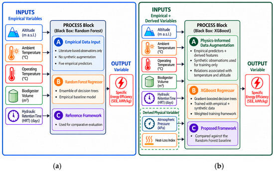
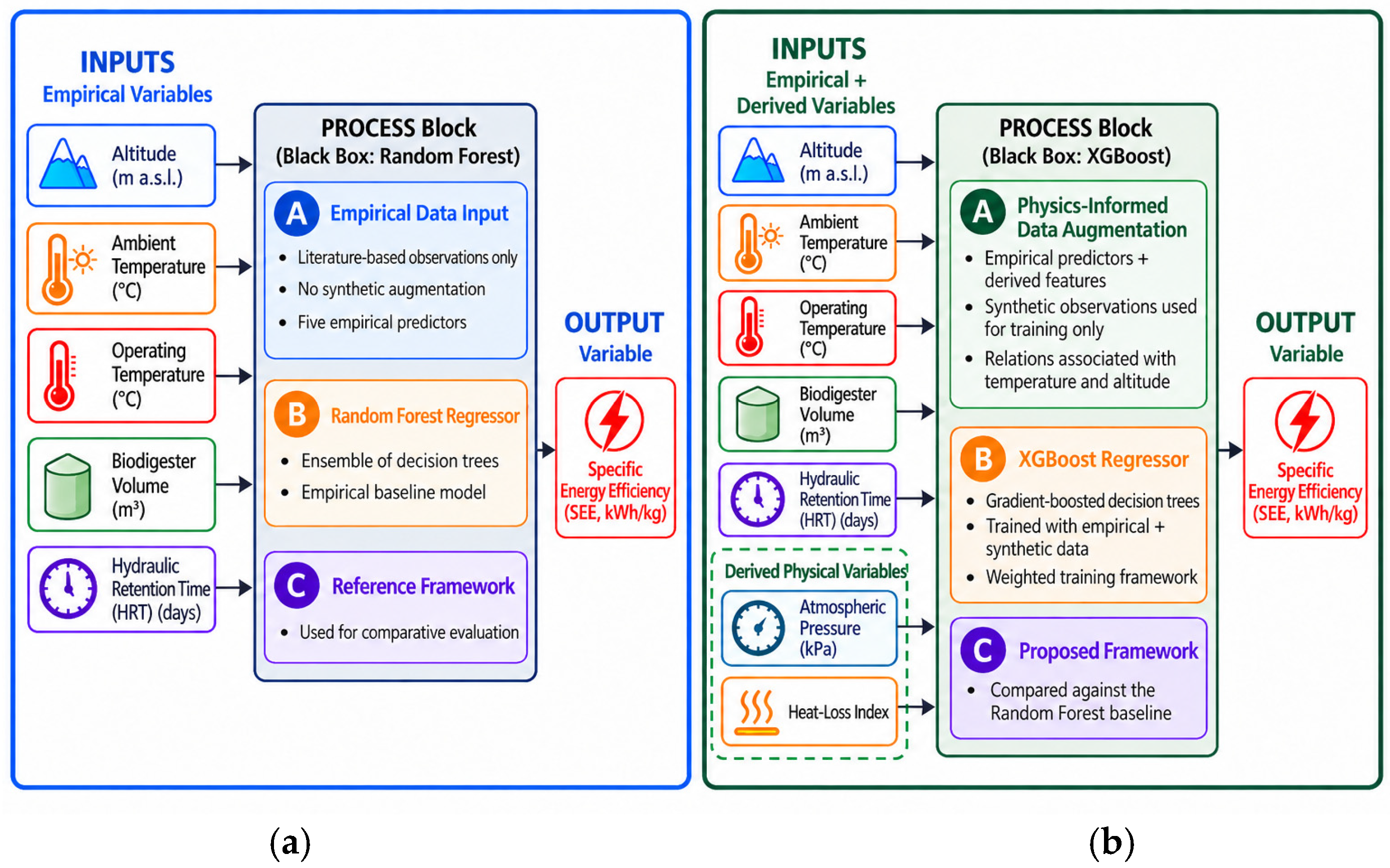
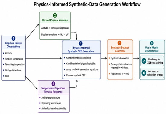
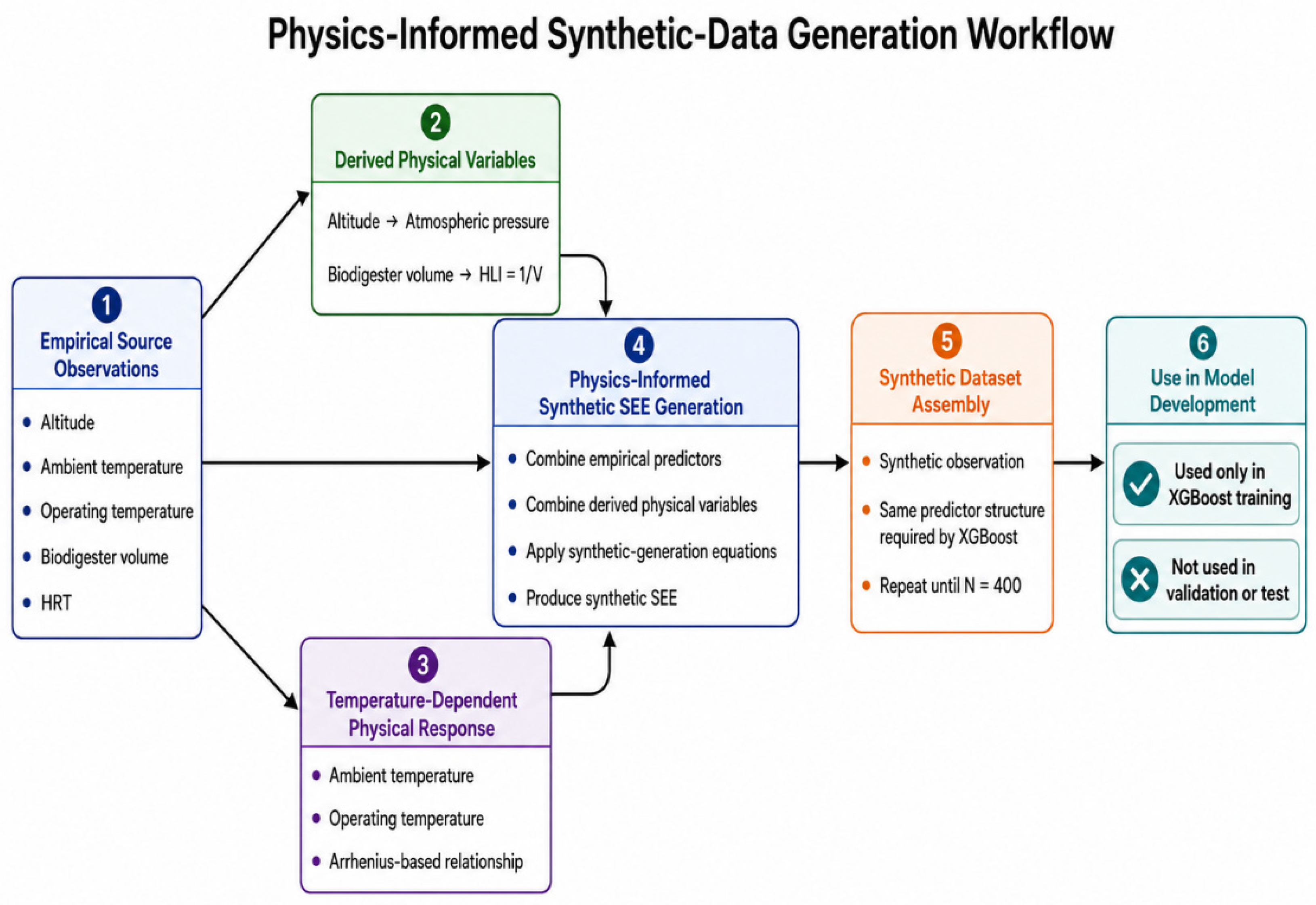
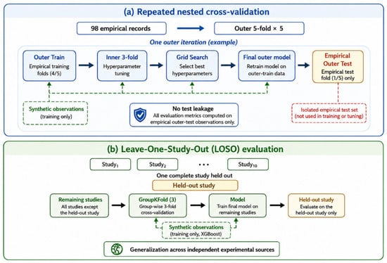
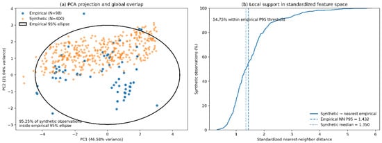
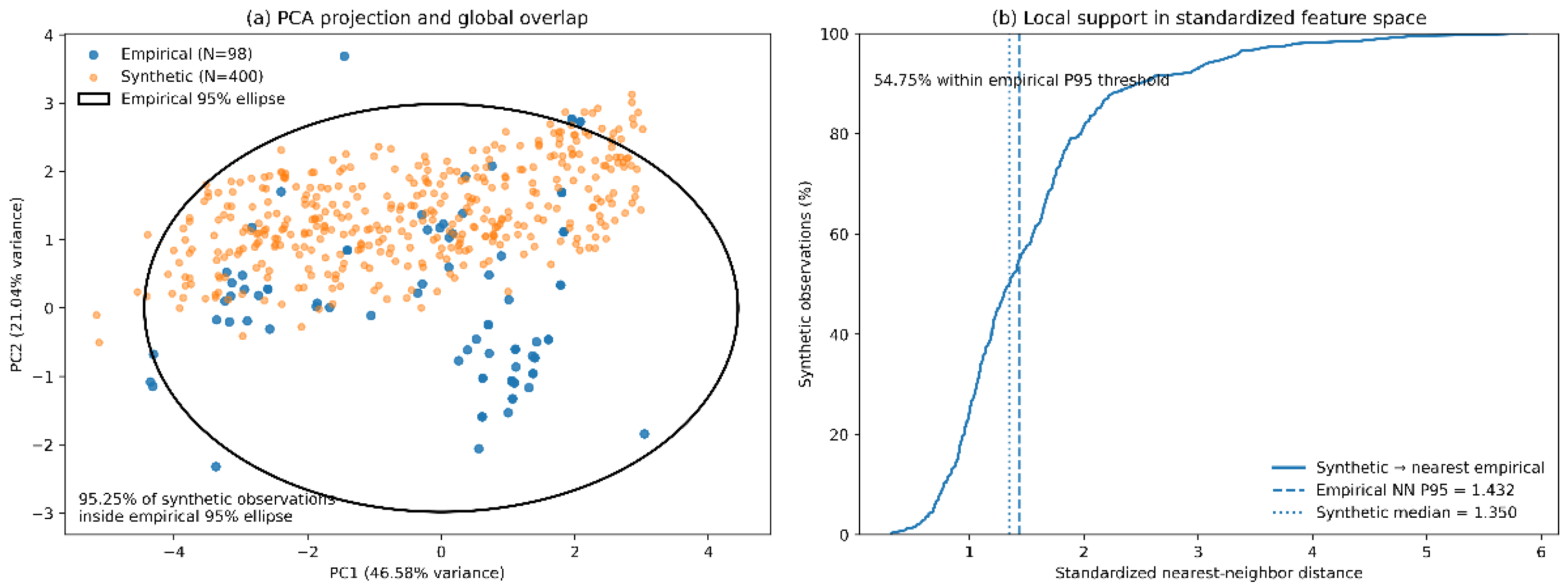
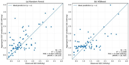
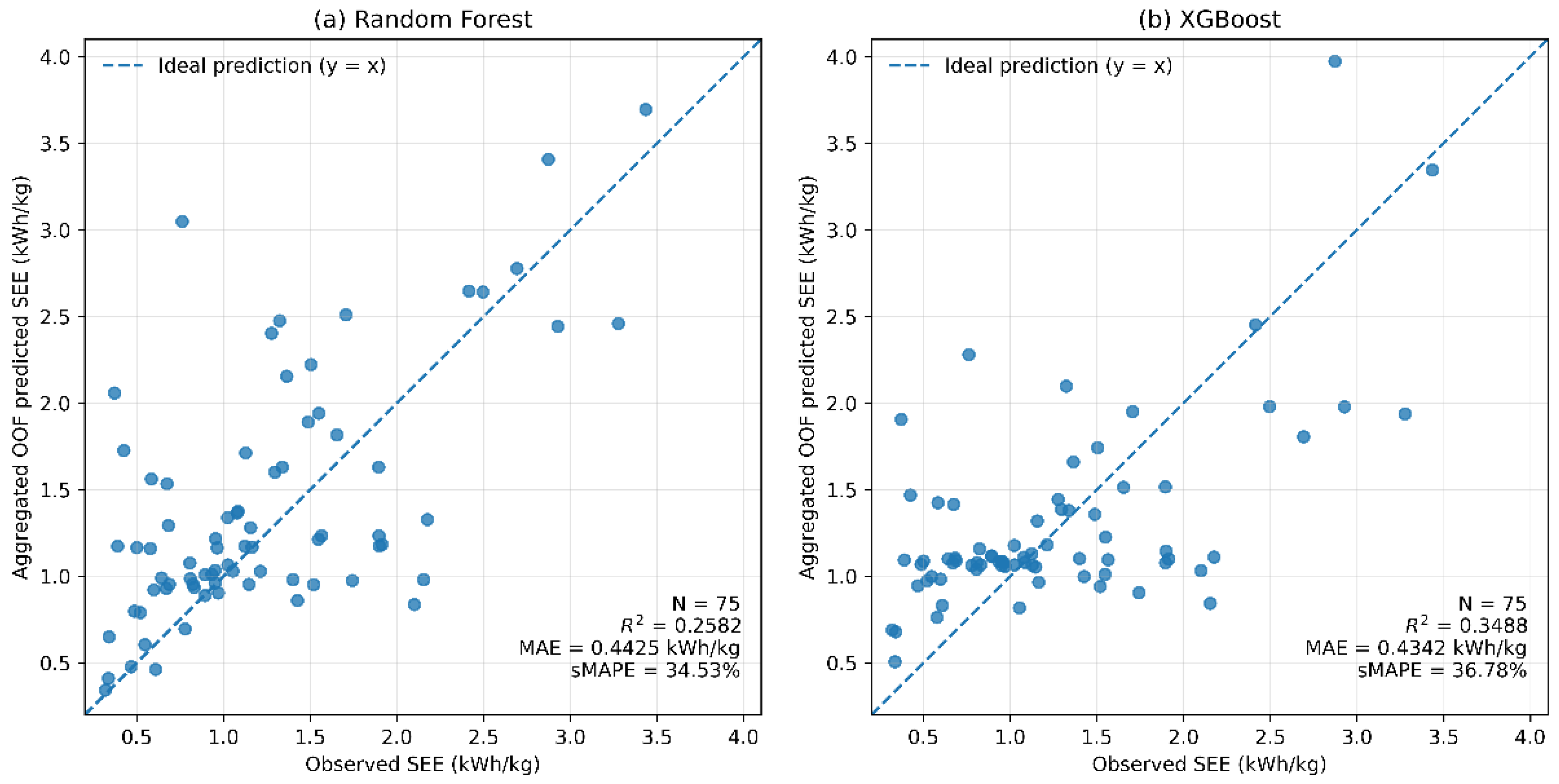
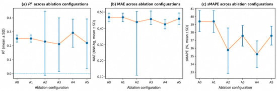
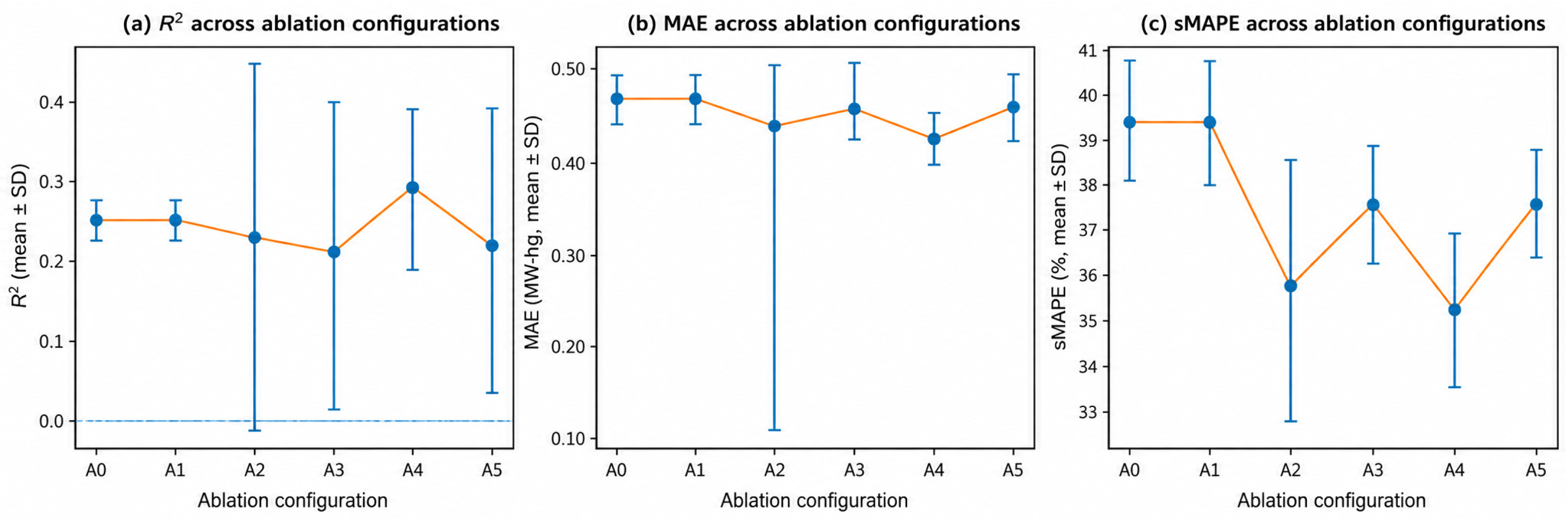
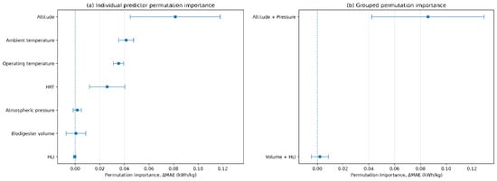
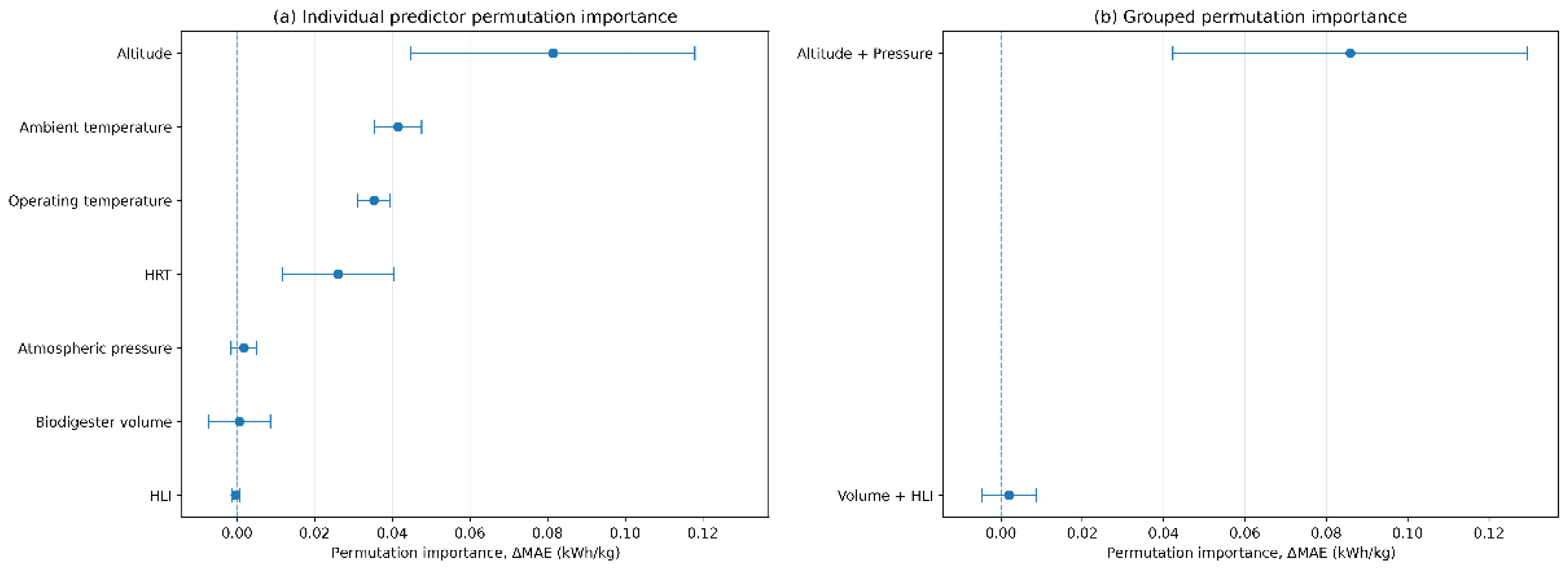

Disclaimer/Publisher’s Note: The statements, opinions and data contained in all publications are solely those of the individual author(s) and contributor(s) and not of MDPI and/or the editor(s). MDPI and/or the editor(s) disclaim responsibility for any injury to people or property resulting from any ideas, methods, instructions or products referred to in the content. |
© 2026 by the authors. Licensee MDPI, Basel, Switzerland. This article is an open access article distributed under the terms and conditions of the Creative Commons Attribution (CC BY) license.