Estimating Cotton Fiber Biological Fineness via High-Throughput Phenotyping

Abstract

Biological fineness of cotton fibers significantly affects spinning performance and yarn quality, yet reliable high-throughput measurement is hindered by morphological variability and limitations of conventional cross-sectional methods. This study developed an automated microscopic imaging system for rapid measurement of cotton fiber phenotypic features from longitudinal-view images, eliminating the need for fiber cross-sectioning. The system integrated a light microscope equipped with a three-axis motorized stage and a high-resolution digital camera for automated scanning and image acquisition. At each (x, y) location, a z-stack of images is captured, and in-focus pixels are fused into a single extended depth-of-field (EDF) image. The EDF images are segmented using Meta’s Segment Anything Model, with prompt points automatically generated from fiber skeletons to separate overlapping fibers. The segmented fiber ribbons are scanned transversely along their centerlines to extract ribbon width, image intensity, and intensity variability, which are incorporated into an empirical model to estimate the fiber perimeter (P). Individual measurements from a slide are aggregated to characterize the distribution of P for each cotton sample. The proposed method demonstrated high repeatability across multiple replicates and independent tests. The estimated P showed strong correlations with AFIS gravimetric fineness (r ≈ 0.80) and with HVI bundle strength (r ≈ −0.95), and a moderate correlation with HVI micronaire (r ≈ 0.65). A preliminary validation test against the cross-sectional method suggested that the perimeter distributions obtained from the estimated and cross-sectional measurements did not differ statistically and were highly correlated (r > 0.960).

1. Introduction

Cotton fiber phenotyping measures geometric features such as biological fineness and ribbon shape. Biological fineness is determined by the perimeter of the fiber cross-section or the diameter of an equivalent circle [1]. Ribbon shape quantifies deformation of the cylindrical structure of the fiber from flattening and twisting. These phenotypic traits are characteristic of cotton varieties or species [1] and are valuable for cotton breeders seeking genetic linkages to improve fiber quality of U.S. cotton.

To obtain reliable measurements of cotton fiber biological fineness, ASTM D1444 was established in 1972 as a standard test method for directly measuring fiber perimeter and cross-sectional area from thin fiber cross-sections [2]. Although the method was withdrawn in 1978 because it was unsuitable for routine commercial testing, its underlying principle remains an important reference for the direct measurement of fiber cross-sectional geometry. Since the 1990s, scientists have worked on establishing protocols for cross-sectioning fibers and capturing images with a digital microscope [3,4,5,6,7]. Special software called the Fiber Image Analysis System (FIAS) was also developed in the early 2010s for the automatic analysis of the cross-sectional images [8,9,10], and was used by scientists to establish a reference dataset from 104 varieties [6,11]. However, the cross-sectioning technique is a time-consuming and expensive procedure, and thus is mainly used to provide direct measurements of cross-sectional features as ground-truth data for calibrating other fiber measurement protocols.

To improve the efficiency of the procedure, efforts to measure the biological fineness from the longitudinal (i.e., side) view were made to avoid fiber cross-sectioning [12,13,14,15]. In these studies, fibers were projected into a 2D image, fiber ribbons were segmented, and the diameter (D) and circularity (C) of individual fibers were estimated by calculating the average of the maximum and minimum ribbon widths (W_max and W_min). To automate this process, Xu et al. used a microscope equipped with a motorized stage and the customized software to capture and analyze the longitudinal images of fiber snippets at multiple positions across a sample slide [16]. The W_max and W_min of over 10,000 fiber snippets per slide could be located in less than two minutes. However, this longitudinal approach is effective only when the fiber ribbon shape looks like a solid rod or is regularly twisted. For fibers, which are either flat or folded axially, such a method would generate significant errors [1]. The ribbons of extremely immature fibers are untwisted. For a flat ribbon, W_max is approximately equal to W_min, which can result in a severe overestimation of D.

The Advanced Fiber Information System (AFIS) and Cottonscope are the two longitudinal measurement systems widely used in the cotton industry [17,18]. Both measure gravimetric fineness in microgram/meter (mtex). AFIS utilizes aerodynamic forces to individualize and move cotton fibers through various sensors where the fiber’s length, width and other parameters are scanned. Because fibers may not be totally separated or straightened in the air passage, AFIS generates very high short-fiber contents (SFC_n > 25%) and super-long fibers in the range of 40 to 60 mm, as indicated in its fiber length distributions [19]. These errors in length measurement would affect AFIS’s mtex calculation. In Cottonscope, a large sample size of fibers (50–60 mg) is cut into 0.7 mm long snippets, and the snippets are spread into water and imaged to be counted for the mtex calculation [18]. Because the actual lengths of the cut snippets vary with the angles between fibers and blade and exposure to water can alter the ribbon structure, these inherent variations are introduced into the mtex calculation. The High Volume Instrument (HVI) is another testing apparatus capable of measuring many cotton fiber properties, including micronaire, using a bundle of cotton fibers rather than individualized fibers [20]. Micronaire provides a ‘ballpark’ value of denier (gravimetric fineness) when divided by a factor of 2.82 [21]. The mtex or denier value is a collective measure of many fibers and thus does not reflect the size of individual fibers.

This research aims to construct a high-throughput fiber phenotyping system, to develop the image acquisition and processing program for reliably estimating the biological fineness of individual cotton fibers from longitudinal-view images and to carry out validation and correlation analyses to evaluate the system’s performance and its potential applications in cotton breeding, parental germplasm selection and fiber development research. Based on challenges identified in our previous studies, this project addresses four critical issues in automated fiber phenotyping: (1) handling out-of-focus fibers in microscopic images; (2) accurately segmenting overlapping or touching fibers; (3) determining the true ribbon width of individual cotton fibers; and (4) estimating the ribbon shape factor required for converting ribbon width to fiber perimeter.

The proposed fiber phenotyping system provides an efficient approach for estimating biological fiber perimeter while avoiding labor-intensive cross-sectioning. The motorized stage allows for the scanning of many fibers (>1000 snippets per slide) in a high-throughput manner. Our success in developing a consistent and rapid fiber phenotyping technique will provide a more reliable measure of fiber fineness and ribbon shapes than those currently provided by Micronaire. With greater breeder access to these more effective measures, they would be better positioned to find genetic linkages and to breed specific maturity traits which would make U.S. cotton higher quality and, therefore, more competitive with man-made fibers.

2. Fiber Phenotyping System

The imaging system used a Nikon LV100ND-U microscope (Melville, NY, USA) equipped with a three-axis motorized stage (a Prior Scientific ES103 3-Axis Motorized Stage System) that automatically controls slide movement in the x–y directions and focal stepping along the z-axis. Images were captured using a 5.9-megapixel color CMOS camera (Nikon DS-Fi3) with a resolution of 1440 × 1024 pixels (or 2880 × 2048 pixels), providing an optical resolution of 0.87 μm/pixel (approximately 29,195 dpi) when used with a TU Plan Fluor EPI 10X objective lens whose numerical aperture is 0.30 and depth of field (DoF) is 3.06 µm. The microscope was illuminated with a 12 V 50 W halogen lamp, and no optical filter was used in the light path. The DS-Fi3 provides a live frame rate of 30 fps at a resolution of 1440 × 1024 pixels, with exposure times ranging from 100 µs to 30 s. To maintain consistent image brightness, the camera’s autoexposure and auto-white-balance functions were enabled.

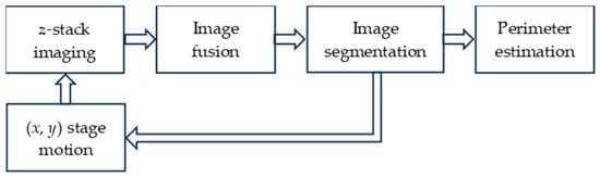
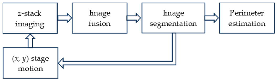
Figure 1 presents a flowchart of the major components of the proposed fiber phenotyping system, which are described in the following sections. Cotton fibers are first cut into approximately 0.5-mm long snippets using a pneumatic cutter, and the snippets are then dispersed by a jet of air into a chamber where they settle randomly onto a microscope slide under gravity, producing a well-separated distribution suitable for imaging [16]. The slide is subsequently placed on the microscope and moved automatically by the x–y motorized stage to acquire images from multiple positions, and the captured images are analyzed and aggregated using specialized software to estimate the biological fineness of thousands of fibers.

Figure 1. Flowchart of cotton fiber phenotyping system.

2.1. Z-Stack Imaging

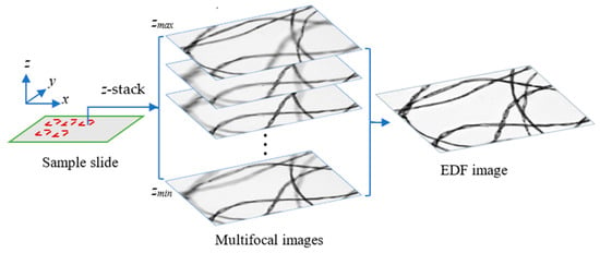
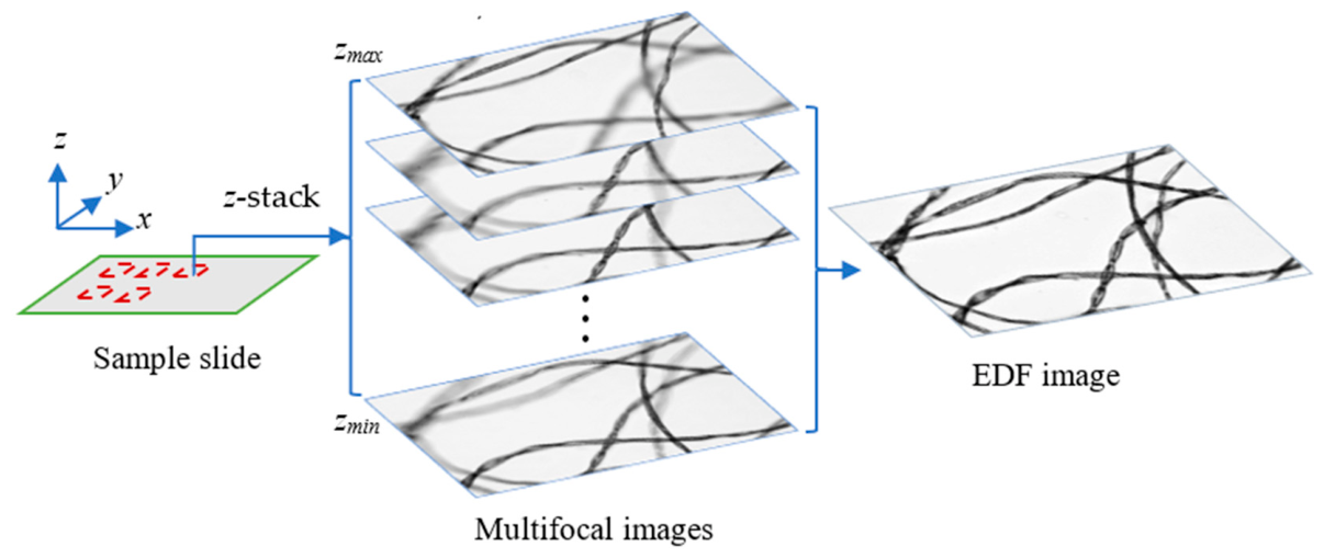
Well-focused microscopic images are essential for accurate cotton fiber phenotyping. At a given magnification, the depth of field of a light microscope is limited and is often insufficient to encompass the full depth occupied by fiber snippets on a microscope slide. Consequently, fiber snippets within the same field of view may lie at different focal depths (z positions), causing some fibers to appear out of focus in a single image captured at a fixed focal plane. To generate a high-fidelity image in which all fiber snippets appear sharply focused, the proposed system employs z-stack imaging to automatically acquire a sequence of images at different focal depths. As illustrated in Figure 2, a slide is divided into a grid of x–y positions that are scanned sequentially by the motorized stage (e.g., in a zigzag pattern). At each position, the stage is synchronized with the camera to capture a sequence of images while stepping from the minimum focal position (z_min) to the maximum focal position (z_max) (e.g., 0–50 μm) with a step size as small as 1 μm. In the experiment, the z-scanning range was set to 150 µm with a z-step size of 10 µm, resulting in 16 image layers at each position. These multifocal images are processed individually to identify in-focus pixels, which are subsequently fused to generate a single extended-depth-of-field (EDF) image, in which all fiber snippets appear sharply focused.

Figure 2. Multifocal images generated by z-stack imaging.

2.2. Multifocal Image Fusion

Multifocal image fusion, also known as extended-depth-of-field (EDF) reconstruction, is a computational imaging technique that combines a sequence of images acquired at different focal depths into a single all-in-focus image. Numerous multifocal image fusion algorithms have been proposed, including methods based on pixel intensity, wavelet transforms, Laplacian pyramids, and deep learning. In this study, we adopted a complex wavelet transform (CWT)-based fusion algorithm because of its superior ability to preserve edge details while minimizing reconstruction artifacts [22,23]. The CWT is approximately shift-invariant and provides enhanced directional representation of image features, enabling more accurate identification and preservation of focused structures, particularly the edges and boundaries of elongated objects such as fiber ribbons.

The CWT-based multifocal image fusion algorithm is founded on the observation that in-focus image regions contain stronger high-frequency components than out-of-focus regions. A sequence of multifocal images is first decomposed using the CWT into one low-frequency sub-band representing the overall image intensity and several high-frequency sub-bands at multiple scales and orientations that capture directional features, such as edges and fine textures. For each corresponding wavelet coefficient across the multifocal image sequence, a focus measure is computed using the absolute value of the coefficient to evaluate the local degree of sharpness. The coefficients with the highest focus measures are then selected to construct a new set of wavelet coefficients, thereby preserving the most sharply focused information from each source image. Consistency checks are performed for the choice of the coefficients. Finally, the fused wavelet coefficients are transformed back using the inverse CWT to reconstruct a single EDF image, in which all fiber snippets appear sharply focused (Figure 2). The resulting EDF image provides a reliable foundation for subsequent fiber ribbon segmentation and biological fineness estimation. In the project, we implemented the CWT-based image fusion algorithm using the open-source library [23], with the required parameter settings listed in Table 1.

Table 1. Parameter settings of the CWT-based image fusion algorithm.

Parameter	Value	Description
wavelet basis	Complex Daubechies	CWT decomposition/reconstruction
consistency	2	Neighbor-consistency filtering
denoise	1.0	Wavelet denoising strength
depthmap_smooth_xy	20	Spatial smoothing of depth map (pixels)
depthmap_smooth_z	40	Z-axis smoothing of depth map (grayscale)
depthmap_threshold	10	Depth-map threshold (grayscale)
halo_radius	20	Halo suppression radius (pixels)
align_flags	ALIGN_KEEP_SIZE	ECC alignment; retain image dimensions
jpgquality	95	Output JPEG quality
remove_bg	0	Background removal disabled
grayscale conversion	PCA-based	Maximizes variance before decomposition

2.3. Image Segmentation

The Segment Anything Model (SAM), developed by Meta AI, is a foundation model for image segmentation that is capable of accurately identifying and delineating objects across a wide range of image domains. Trained on the SA-1B dataset, which contains more than one billion segmentation masks from 11 million images, SAM demonstrates strong zero-shot generalization, enabling it to segment previously unseen objects without task-specific retraining [24]. Given an input image and optional prompts, such as points, bounding boxes, or masks, the model can extract object boundaries from complex backgrounds with high robustness.

To further improve segmentation quality, an enhanced version of SAM was designed to achieve more accurate boundary localization and fine-detail segmentation while retaining the strong zero-shot generalization capability [25]. SAM-HQ incorporates a lightweight high-quality output decoder and is further trained using the HQSeg-44K dataset, which contains approximately 44,000 high-quality segmentation masks. Compared with the original SAM, SAM-HQ produces more precise boundaries for thin and complex structures, making it particularly well suited for segmenting elongated cotton fiber snippets in microscopic images.

In this study, the fiber EDF images were first converted into binary images using the Otsu thresholding algorithm, and one-pixel-thick centerlines of fiber snippets were extracted using the Guo-Hall algorithm. Both algorithms were implemented in the industry-standard OpenCV library (OpenCV–4.12.0) [26]. Skeletal pixels away from ends (those having only 1 neighbor) and joints (those having more than 3 neighbors) were then selected as prompt points and provided to SAM-HQ together with the corresponding EDF image. We implemented the SAM-HQ model for image segmentation using the open-source SAM-HQ repository [27], with the required parameter settings listed in Table 2.

Table 2. Parameter settings of the SAM-HQ model.

Parameter	Value
backbone	vit_l
points_per_side	32
points_per_batch	64
pred_iou_thresh	0.88
stability_score_thresh	0.95
min_instance_area	0
max_instance_area_ratio	0.1
overlap_thresh	0.5
multimask_output	false
device	cuda

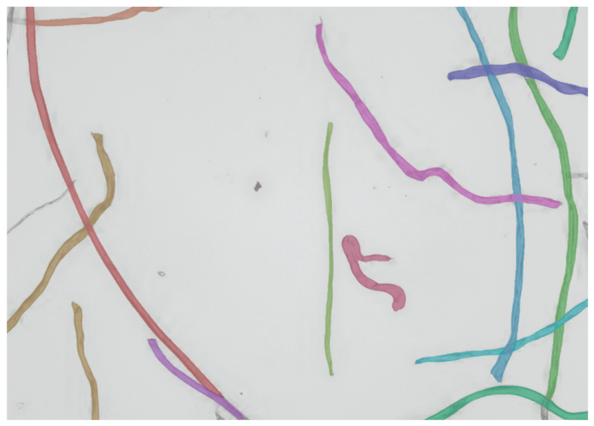
As shown in Figure 3, SAM-HQ accurately delineated the boundaries of elongated and irregularly shaped fiber snippets, substantially reducing the need for manual annotation and generating reliable segmentation masks for subsequent measurements of ribbon width, perimeter estimation, and biological fineness analysis.

Figure 3. Fiber snippets segmented by SAM-HQ using fiber skeletal pixels as prompts are shown in different colors.

2.4. Ribbon Width Measurement

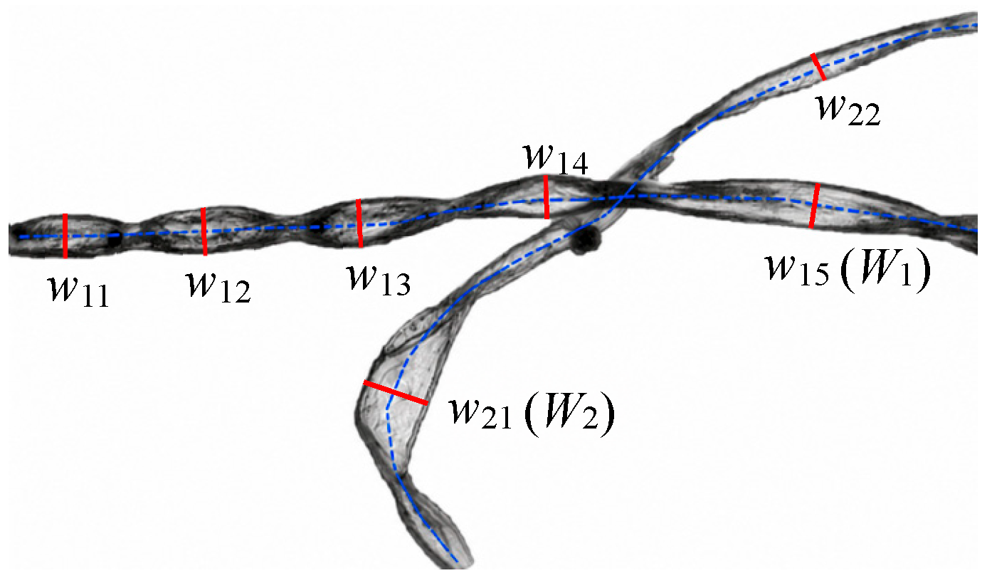
Because cotton fibers are naturally twisted and folded along their longitudinal axes, the projected ribbon width in a longitudinal-view image varies continuously along the centerline of each fiber snippet. However, the true ribbon width and corresponding perimeter at any cross section are intrinsic fiber properties determined by the cotton variety rather than by the fiber’s orientation in the image. Only at locations where the ribbon is oriented perpendicular to the optical axis of the microscope does the projected width attain a local maximum. Therefore, the global maximum of all local maximum widths is regarded as the true ribbon width of the fiber snippet. Figure 4 illustrates two cotton fiber ribbons and their corresponding centerlines extracted using the skeletonization algorithm. One fiber exhibits a relatively uniform twisting pattern and contains five similar local maximum ribbon widths (w₁₁, … and w₁₅), whereas the other fiber is more folded and exhibits two distinct local maximum widths (w₂₁ and w₂₂). The true ribbon widths of the two fiber snippets, denoted by W₁ and W₂, are identified as w₁₅ and w₂₁, respectively, corresponding to the global maximum among the local maximum widths of each fiber.

Figure 4. Fiber ribbon width measurements. The blue dashed lines are the centerlines of two fibers).

2.5. Fiber Perimeter Estimation

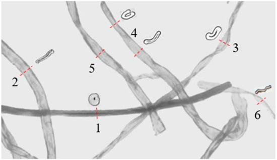
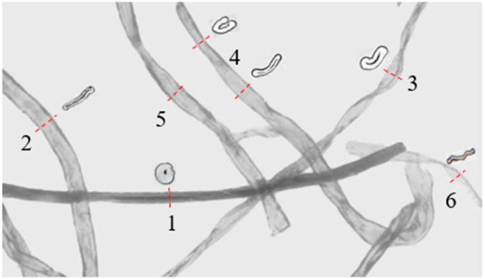
Figure 5 illustrates a longitudinal image of representative cotton fiber snippets, labeled 1–6, exhibiting varying degrees of twisting, folding, and maturity. To facilitate interpretation, representative cross-sectional shapes are superimposed on the corresponding fibers. Fiber 1 is a fully mature fiber that appears nearly cylindrical and solid, with an almost filled lumen. Fiber 2 is an immature fiber with a collapsed lumen and no apparent twisting or folding. Fiber 3 is a regularly twisted fiber with a ribbon-like morphology. Fibers 4 & 5 are immature fibers that are flattened and partially folded. Fiber 6 is an extremely immature fiber that appears as a thin, flattened ribbon. Fibers with similar ribbon widths (W) may possess markedly different perimeters because of differences in their cross-sectional morphologies. Consequently, estimating the shape factor from ribbon image features is a critical step for perimeter estimation.

Figure 5. Longitudinal image of cotton fiber snippets with corresponding cross-sectional shapes illustrating different fiber morphologies.

From this image, the effects of fiber morphology on image appearance can be observed: (1) the overall ribbon intensity increases with lumen size (e.g., Fiber 1 < Fiber 2), because a larger lumen corresponds to a thinner cellulose wall and greater light transmission; (2) the spatial variation in ribbon intensity increases with the degree of fiber twisting (e.g., Fiber 3 > Fiber 5); and (3) fibers with little or no twisting exhibit relatively uniform intensity along their lengths (e.g., Fibers 1 and 6). These relationships were consistently observed in numerous longitudinal images. To quantitatively characterize fiber morphology, the following image features are extracted from each segmented fiber ribbon:

• Mean intensity ($I$): the average pixel intensity measured along the scan line used to determine the ribbon width ($W$). This feature reflects the translucency of the fiber and is therefore related to the thickness of the cellulose wall.
• Intensity coefficient of variation ($I_{cv}$): the coefficient of variation in the pixel intensities along the axis of the segmented fiber ribbon ($I_{cv}=I_{sd }/{ I}_{mean}$), which reflects the degree of fiber twisting.
• Background intensity ($I_b$): the average intensity of the non-fiber background, providing an upper reference for comparison with extremely immature, nearly transparent fibers.
• Minimum fiber intensity ($I_{min}$): the average intensity of fully mature fibers, providing a lower reference for comparison with nearly opaque fibers having very small or no visible lumen.

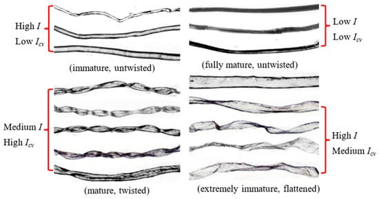
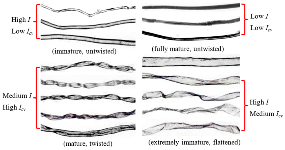
To establish the relationship between ribbon image features and fiber morphology, we collected fiber snippets exhibiting a wide range of maturity levels and twisting patterns and grouped them into four maturity categories according to the cotton classification described in [28]. Figure 6 illustrates representative fiber ribbons from these four categories, each exhibiting distinct combinations of ribbon width, intensity, and intensity variation. Once the image features of an individual fiber ribbon are extracted, its shape factor (a) can be estimated using a simple linear model described in the following section. Because fiber perimeter (P) is proportional to ribbon width for a given cross-sectional morphology, P can be expressed as P = a × W, where W is the true ribbon width.

Figure 6. Representative cotton fiber snippets with varying degrees of maturity and twisting, and corresponding image features.

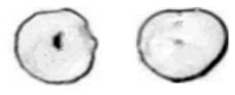
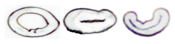
During the first three stages of cotton fiber development (initiation, elongation, and secondary wall thickening), a fiber retains a nearly cylindrical shape while elongating and depositing cellulose inward along the secondary wall. During the fourth stage (maturation), water contained within the lumen and associated with the cellulose molecules is gradually lost, causing the cylindrical structure to collapse and twist along its longitudinal axis. If fiber development ceases before the secondary wall thickening stage is complete, the fiber remains extremely immature, and its cylindrical structure collapses into a thin, flattened ribbon, as illustrated in the first column of Table 3. In this limiting case, the shape factor is a = 2, and the ribbon intensity approaches that of the image background (I ≈${ I}_b$) because the thin cellulose wall is nearly transparent. In contrast, if the lumen is completely filled with cellulose by the end of the thickening stage, the fiber cross section approaches a solid circle, as shown in the second column of Table 3. In this limiting case, the shape factor reaches a = π, and the ribbon exhibits the minimum intensity (I ≈ $I_{min}$) because the thick cellulose wall transmits the least amount of light. Most cotton fibers exhibit morphologies intermediate between these two limiting cases, with partially or fully collapsed cross-sections (the 3rd column in Table 3). Depending on the degree of longitudinal twisting, their cross-sections typically appear kidney-shaped, whereas fibers with little or no twisting tend to exhibit oval or elliptical cross-sections. For intermediate fiber morphologies, the shape factor can be estimated by linearly interpolating between the two limiting cases using the normalized ribbon intensity and incorporating the effect of fiber twisting through the intensity coefficient of variation ($I_{cv}$):

$$a=\left[2+\left(\pi -2\right){\displaystyle \frac{I_b- I}{I_b- I_{min}}}\right]\left(1+I_{cv}\right)$$

(1)

where the first term estimates the shape factor based on cell wall thickness, and the second term accounts for the increase in apparent perimeter associated with longitudinal twisting. As a simple and physically intuitive first-order approximation, linear interpolation is adopted because developing an alternative nonlinear relationship would require additional cases representing a broader range of cross-sectional shapes. Because several terms in Equation (1) are related to image intensity, consistent illumination and imaging conditions are important for reliable estimation. Accordingly, auto-white balance and auto-exposure were applied before image acquisition to maintain consistent imaging conditions throughout the experiments.

Table 3. Cross-sectional shapes of cotton fibers.

Flattened;	Solid;	Compressed;
Nearly transparent	Nearly opaque	Translucent
a = 2; I ≈ Ib	a = π; I ≈ Imin	a = f(I, Ib, Imin, Icv)

3. Experiment

3.1. Materials

Thirteen cotton varieties representing four cultivated cotton species were obtained from the USDA-ARS National Plant Germplasm System cotton collection at College Station, TX [29]. The cotton materials studied included three Gossypium herbaceum varieties (A1-0029, A1-0143, and A1-0167), three G. arboreum varieties (A2-0061, A2-0190, and A2-1457), three G. barbadense varieties (GB-0245, GB-1336, and STD-04), and four G. hirsutum varieties (SA-1330, SA-1419, SA-1766, and STD-03). STD-03 and STD-04 are the historical genetic standards for G. hirsutum and G. barbadense named ‘TM-1’ and ‘3-79’, respectively.

The cotton varieties were grown in the field in College Station, TX, and bolls from four lots were manually harvested in October 2024 and subsequently processed using a laboratory saw gin. The resulting fiber samples were evaluated at Cotton Incorporated using two widely accepted cotton fiber testing systems manufactured by Uster Technologies AG (Uster, Switzerland): the High Volume Instrument (HVI) and the Advanced Fiber Information System (AFIS). As summarized in Table 4, the AFIS measurements include fineness and maturity ratio (MR), whereas the HVI measurements include bundle strength and micronaire. AFIS fineness is expressed as gravimetric fineness in units of mtex. The means (M) and standard deviations (SD) of each metric reported in the table were calculated from the four lots (reps) of each cotton variety. The cotton samples span a broad range of fiber properties, providing a diverse dataset for evaluating the performance and robustness of the proposed fiber phenotyping system.

Table 4. Fiber properties of the 13 cotton varieties measured by AFIS and HVI.

Species	Variety	AFIS				HVI
		Fineness (mtex)		Maturity Ratio		Strength (g/tex)		Micronaire
		M	SD	M	SD	M	SD	M	SD
G. herbaceum	A1-0029	194.25	3.30	0.98	0.01	29.60	0.87	5.81	0.09
	A1-0143	211.75	5.12	0.93	0.02	23.48	0.57	6.01	0.21
	A1-0167	187.00	1.41	0.85	0.01	23.18	0.83	4.60	0.43
G. arboreum	A2-0061	197.00	5.60	0.93	0.03	24.28	0.46	5.55	0.20
	A2-0190	158.75	6.18	0.94	0.03	31.48	3.24	3.32	0.47
	A2-1457	178.00	4.08	0.99	0.02	28.50	0.22	5.03	0.19
G. barbadense	GB-0245	130.50	1.91	0.90	0.01	34.45	1.43	2.52	0.16
	GB-1336	147.50	1.73	0.95	0.01	36.95	1.27	3.86	0.18
	STD-04	136.50	1.29	0.92	0.01	39.00	1.62	3.14	0.20
G. hirsutum	SA-1330	164.25	6.85	0.95	0.03	30.35	1.18	4.17	0.37
	SA-1419	162.75	4.65	0.90	0.02	26.85	0.96	3.61	0.28
	SA-1766	163.00	7.87	0.94	0.04	30.03	1.73	3.99	0.51
	STD-03	164.00	4.69	0.95	0.02	31.70	1.48	4.08	0.47

Note: M and SD denote mean and standard deviation, respectively.

3.2. Methods

To evaluate the proposed method, fibers from each cotton variety were sampled and manually drawn into a bundle, which was then cut into approximately 0.5-mm-long snippets and dispersed onto a microscope slide using the pneumatic cutter [16]. The density of fiber snippets on the slide was controlled by varying the number of cuts made by the cutter. Accordingly, three slides, designated S1, S2, and S3, were prepared for each variety using one, two, and three cuts, respectively, resulting in low-, medium-, and high-density snippet distributions. The microscope’s motorized x–y stage was programmed to scan the slide at 20 × 10 positions with a 1-mm step interval, yielding 200 EDF images per scan. The 200 EDF images acquired from each scan yielded approximately 800–3500 segmented fiber snippets, depending on the snippet density on the slide. Each slide was scanned twice on the microscope at different times. The second scan was performed independently and did not start from the same x–y position as the first scan. Consequently, the two image datasets contained overlapping but non-identical fiber snippets, providing an independent test of measurement repeatability.

The fiber phenotyping software was developed in C++ and compiled using MSVC 2022 on Windows. All image acquisition, EDF fusion, and segmentation were performed on a workstation running Windows 11 equipped with an Intel Core i9-14900K CPU, 64 GB DDR5 RAM (4800 MT/s), and an NVIDIA GeForce RTX 4090 GPU (24 GB VRAM). On average, processing a single EDF image required approximately 6 s for z-stack image acquisition, 4 s for CWT-based image fusion, 40 s for SAM-HQ segmentation of the fused image, and 10 s for measurement of the segmented image.

Table 5 summarizes the fiber perimeters of the 13 cotton varieties measured using the proposed fiber phenotyping system. For each variety, the mean ($M$) and standard deviation ($SD$) of the estimated fiber perimeters were calculated using all measurements obtained from the three slides across the two independent scans. Repeatability was evaluated at two levels: (1) within-test repeatability, by comparing the three replicate slides acquired during the same scan, and (2) between-test repeatability, by comparing the results of the two independent scans. The proposed phenotyping system was further validated by evaluating the correlations between the mean fiber perimeter values and the corresponding fiber properties measured by the AFIS and HVI systems.

Table 5. Fiber perimeters of cotton varieties measured by the fiber phenotyping system.

Variety	Test 1					Test 2
	S1	S2	S3	M	SD	S1	S2	S3	M	SD
A01-029	53.68	55.02	53.53	54.49	15.21	51.54	55.68	53.95	53.72	15.22
A01-143	56.32	57.52	60.00	57.95	15.59	54.11	57.93	60.36	57.47	15.41
A01-167	62.49	61.19	60.00	61.23	15.40	60.59	62.89	59.29	60.92	15.73
A02-0061	59.93	61.21	58.02	59.72	16.15	58.68	61.73	58.34	59.58	16.31
A02-0190	56.43	57.68	54.14	56.08	16.37	54.10	58.11	53.94	55.38	16.83
A02-1457	54.93	55.38	52.32	54.21	16.79	55.25	55.02	51.38	53.88	17.10
GB-0245	51.29	52.05	49.29	50.88	17.22	50.34	50.52	48.34	49.73	17.03
GB-1336	50.94	48.39	51.14	50.16	17.30	50.42	48.87	51.25	50.18	16.69
STD-04	48.83	47.27	48.25	48.12	16.40	49.51	48.94	48.76	49.07	16.26
SA-1330	51.88	52.99	50.93	51.93	16.97	51.91	52.44	50.85	51.73	16.45
SA-1419	54.90	56.45	54.49	55.28	16.66	53.10	53.10	54.66	53.62	16.23
SA-1766	55.22	55.21	53.15	54.53	16.69	52.27	55.19	52.53	53.33	16.47
STD-03	52.95	53.05	52.19	52.73	16.41	52.38	52.97	52.10	52.48	16.25

4. Results and Discussion

4.1. Repeatability Across Different Snippet Densities

Table 6 presents the Pearson correlation coefficients ($r$) of fiber perimeter measurements obtained from pairwise comparisons among the three replicate slides (S1, S2, and S3) within each of the two independent tests. The correlation coefficients ranged from 0.78 to 0.95, indicating good repeatability of the proposed phenotyping system despite substantial differences in fiber snippet density on the microscope slides. The p-values corresponding to the correlation coefficients (values in parentheses in the table) were all below 0.001, indicating that all six correlations were statistically significant. The highest correlations were observed between S1 and S2 (low- and medium-density slides), with $r=0.95$ in Test 1 and $r=0.92$ in Test 2. The lowest correlations occurred between S1 and S3 in the Test 1 ($r=0.87$), and between S2 and S3 in the Test 2 ($r=0.78$). Overall, the high-density slide (S3) tended to exhibit slightly lower correlations with the lower-density slides, suggesting that increased snippet density may have a modest effect on measurement consistency. Nevertheless, all correlation coefficients exceeded 0.78, indicating that the proposed system provides highly repeatable perimeter measurements across a wide range of sample densities.

Table 6. Pearson correlation coefficients of fiber perimeters in the two tests.

Slide	Test 1		Test 2
	S2	S3	S2	S3
S1	0.95 (6.76 × 10−7)	0.87 (1.11 × 10−4)	0.92 (8.45 × 10−6)	0.86 (1.63 × 10−4)
S2		0.89 (4.59 × 10−5)		0.78 (1.66 × 10−3)

Note: values in parentheses are p-values for correlations.

Paired t-tests also showed no significant differences between the measurements obtained from any two of the three slides (p > 0.05), indicating that no significant effect of fiber snippet density on the estimated perimeter measurements was detected. In Test 1, the p-values were 0.457, 0.074, and 0.107 for the S1 vs. S2, S1 vs. S3, and S2 vs. S3 comparisons, respectively. Similarly, in Test 2, the corresponding p-values were 0.578, 0.074, and 0.107, respectively. These results demonstrate that the image fusion, fiber segmentation, and perimeter estimation procedures are robust to variations in sample loading.

4.2. Repeatability Across Tests

When all fiber perimeter measurements from the three replicate slides were combined within each test, the correlation coefficient between the two independent tests reached $r=0.96$, demonstrating excellent between-test repeatability of the proposed phenotyping system. This high correlation is particularly noteworthy because the two scans analyzed different subsets of fibers from the same slides rather than repeated measurements of the identical fiber snippets.

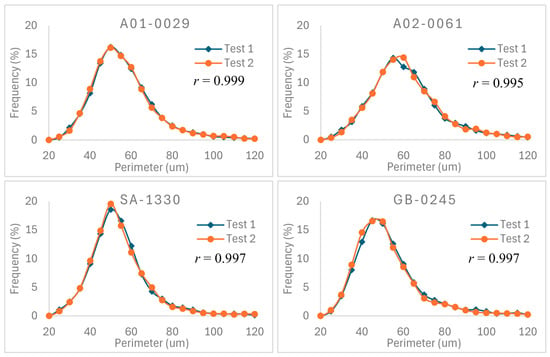
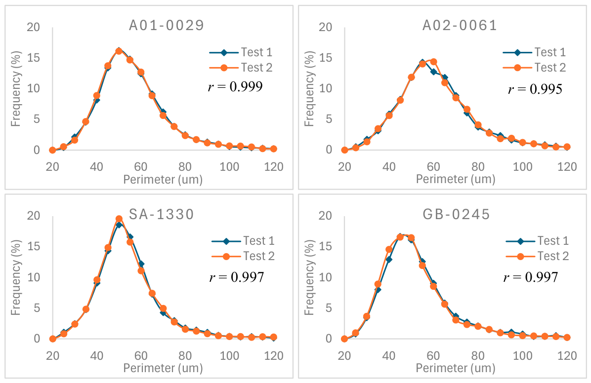
A more detailed evaluation was performed by comparing the fiber perimeter distributions obtained from the two independent tests for each cotton variety. The Pearson correlation coefficients between the corresponding distributions ranged from 0.995 to 0.999, indicating nearly identical distribution shapes across repeated measurements. Figure 7 presents the perimeter distributions of four representative varieties selected from four cotton species. With only minor differences near the distribution peaks, the two distributions for each variety exhibited excellent agreement. These results demonstrate that the proposed fiber phenotyping system provides highly reproducible estimates of both the mean fiber perimeter and the entire population distribution, making it well suited for quantitative comparisons among cotton varieties. The p-values from the paired tests on the two distributions of the four selected varieties were equal to 1.00, indicating complete consistency between Test 1 and Test 2.

Figure 7. Fiber perimeter distributions of four cotton varieties (each representing a different cotton species) in the two repeated tests conducted at different times.

4.3. Comparison of Perimeter Distributions Among Cotton Species

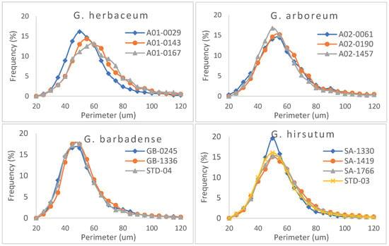
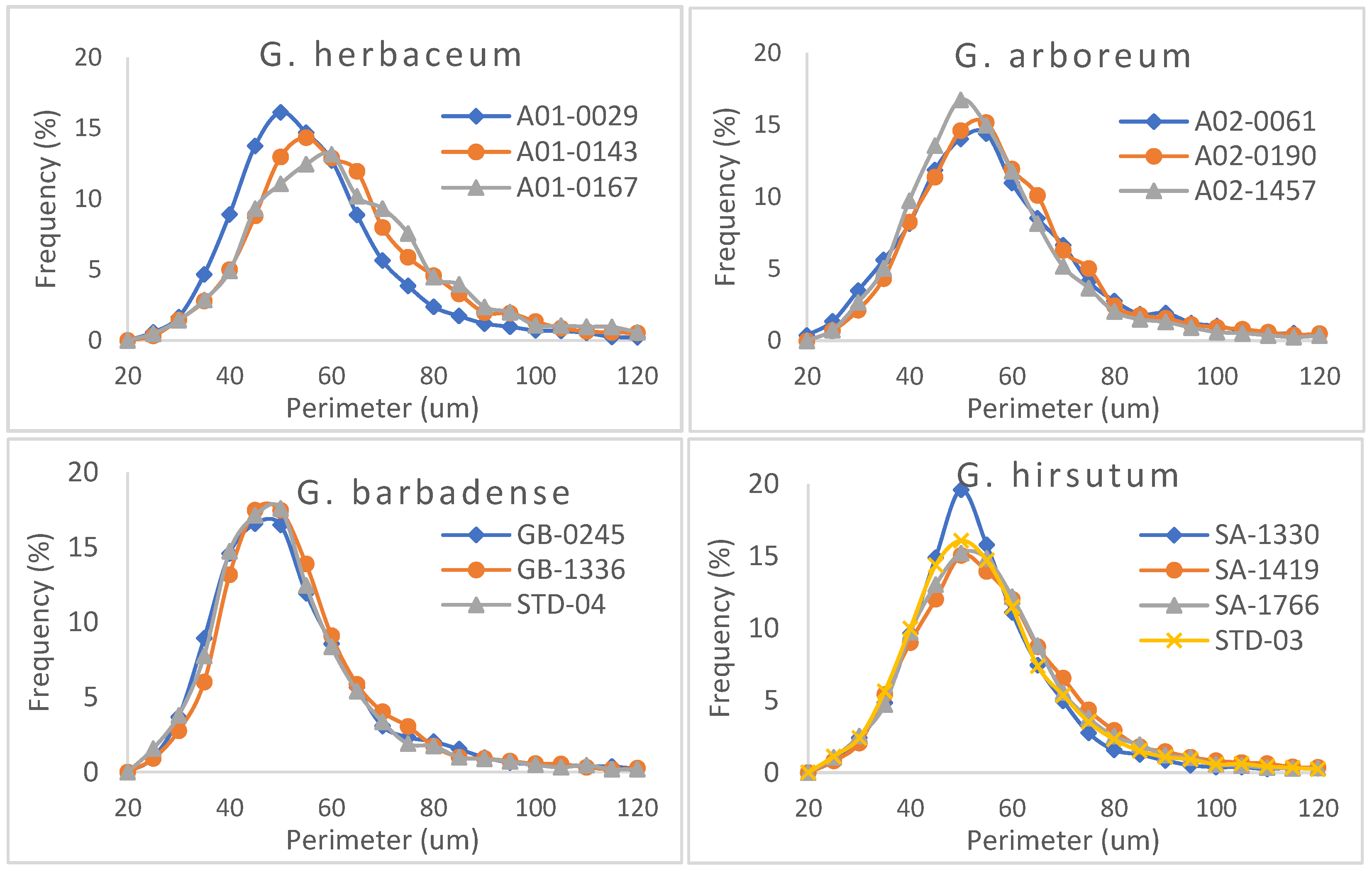
To investigate the biological relevance of the perimeter measurement, fiber perimeter distributions were compared among varieties within each of the four cotton species (Figure 8). The four species exhibited distinct distribution characteristics. Overall, the three G. herbaceum species tended to exhibit the largest fiber perimeters, whereas the G. barbadense species generally had the smallest perimeters. The G. arboreum and G. hirsutum species displayed intermediate distributions. Within each species, individual varieties also showed discernible differences in their perimeter distributions, reflecting genetic variation in fiber fineness. These results demonstrate that fiber perimeter provides a sensitive phenotypic trait for differentiating both cotton species and varieties, while the complete perimeter distribution offers more comprehensive information than a single mean value alone.

Figure 8. Fiber perimeter distributions of cotton varieties in four species.

Friedman test, a nonparametric test for 3+ paired datasets, was applied to quantify how the fiber perimeter distributions of three or four cotton varieties in each of the four species differ statistically. As shown in Table 7, the p-values of the Friedman tests for the four species were all greater than 0.05, indicating no statistically significant differences among the fiber-perimeter distributions of cotton varieties within each species at α = 0.05. However, the p-value for G. hirsutum (0.052) was very close to, but slightly above, the significance threshold. To assess concordance in the rankings of the fiber-perimeter distributions among the three measurements within each species, Kendall’s coefficient of concordance (W) was calculated (0 ≤ W ≤ 1). The W values for G. herbaceum and G. barbadense were below 0.10, indicating very weak concordance among the three distributions within each species. The W values for G. arboreum and G. hirsutum were within the 0.10–0.30 range, indicating weak concordance among the distributions within each species.

Table 7. Friedman test of fiber perimeter distributions among cotton varieties in each species.

Species	G. herbaceum	G. arboreum	G. barbadense	G. hirsutum
Variety	A1-0029, A1-0143, A1-0167	A2-0061, A2-0190, A2-1457	GB-0245, GB-1336, STD-04	SA-1330, SA-1419, SA-1766, STD-03
df	2	2	2	3
Statistics ${\chi }^2$	3.60	4.30	1.60	7.74
p-values	0.165	0.116	0.449	0.052
Kendall’s W	0.090	0.108	0.040	0.129

4.4. Validation Against Cross-Sectional Measurements

Two fiber samples were selected for a preliminary test to compare the estimated perimeters obtained using the proposed method with those measured using the cross-sectional method [8,9], which served as the ground truth. The cross-sectioning of the samples was performed at the Fiber & Polymer Research Institute of Texas Tech University. Because both methods are destructive to the fibers, it is not possible to perform both measurements on the same fiber and generate paired observations. Therefore, the Mann–Whitney U test, a nonparametric statistical test, was used to determine whether the two unpaired perimeter datasets differed significantly. Table 8 presents the fiber perimeter statistics and Mann–Whitney U test results for the two samples. The numbers of fibers measured using the estimation model and the cross-sectional method were 5210 and 3486, respectively, for Sample 1, and 4306 and 3775, respectively, for Sample 2. The differences in mean fiber perimeters between the two methods were 4.46 µm (8.80%) for Sample 1 and 3.48 µm (7.16%) for Sample 2.

Table 8. Fiber Perimeter Statistics and Mann–Whitney U Test Results.

	Sample 1		Sample 2
	Estimated	Cross-Sectional	Estimated	Cross-Sectional
Number	5210	3486	4306	3775
Median (µm)	53.26	50.63	48.81	47.95
IQR (µm)	44.16–63.41	43.54–57.11	41.50–58.78	40.10–55.52
Mean (µm)	55.15	50.69	52.06	48.58
Difference (%)	8.80		7.16
U	10,330,120.50		8,832,039.50
p-value	1.33 × 10−27		1.664 × 10−11

For Sample 1, a two-sided Mann–Whitney U test demonstrated a statistically significant difference between the estimated and cross-sectional datasets (U = 10,330,120.5, p < 0.001). The Hodges–Lehmann estimated location difference was 3.19 µm (95% CI: 2.61–3.77 µm), indicating that the estimated dataset was approximately 3.19 µm higher than the cross-sectional dataset, with the likely difference ranging from 2.61 to 3.77 µm. The corresponding rank-biserial correlation (r_b), used as a measure of effect size associated with the Mann–Whitney U test, was 0.138 (95% CI: 0.114–0.162), indicating a small effect, i.e., the degree of rank separation between the estimated and cross-sectional measurements was small. The AUC was 0.569, suggesting that a randomly selected observation from the estimated dataset had approximately a 56.9% probability of being higher than a randomly selected observation from the cross-sectional dataset. Both r_b of 0.138 and AUC of 0.569 reveal that the estimated perimeter tends to be higher than the cross-sectional perimeter, but the separation between the two datasets is relatively small.

For Sample 2, the Mann–Whitney U test indicated a statistically significant difference between datasets A and B (U = 8,832,039.5, p < 0.001). The Hodges–Lehmann estimated difference was 1.95 μm (95% CI: 1.16–2.78 μm), while the corresponding rank-biserial correlation r_b was 0.087 (95% CI: 0.053–0.123), indicating a negligible (very small) effect size. An AUC of 0.543 indicates that the estimated perimeter has a 54.3% probability of being higher than the cross-sectional measurement, suggesting that the discrimination between the two measurements is close to neutral.

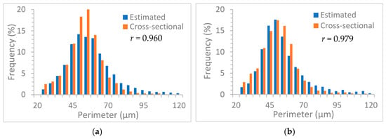
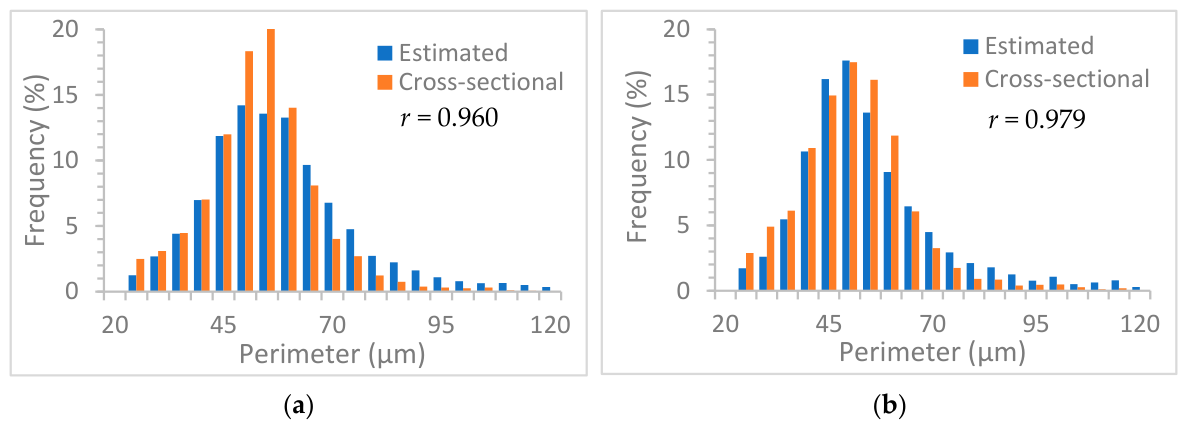
To examine fine differences between the estimation model and the cross-sectional method across the fiber perimeter range of (20–120) μm, the fiber perimeter distributions, i.e., the frequencies of fibers within certain perimeter intervals, were plotted for Sample 1 in Figure 9a and Sample 2 in Figure 9b. Although apparent differences between the two distributions can be observed at some locations in Figure 9a,b, the Wilcoxon signed-rank tests for Sample 1 (p = 0.261 > 0.05) and Sample 2 (p = 0.452 > 0.05) did not suggest a systematic difference between the distributions of the estimated and cross-sectional measurements. The paired distributions were also highly correlated, with correlation coefficients (r) of 0.960 for Sample 1 and 0.979 for Sample 2. Overall, these preliminary results provide encouraging evidence that the proposed estimation method produces fiber perimeter distributions that are consistent with those obtained from cross-sectional measurements.

Figure 9. Distributions of fiber perimeters measured with the estimation model and cross-sectional method for Sample 1 (a) and Sample 2 (b).

4.5. Validation Against AFIS and HVI Measurements

The fiber perimeter measurements obtained using the proposed phenotyping system were compared with conventional fiber quality measurements generated by the AFIS and HVI systems through correlation analysis. Pearson correlation coefficients (r) were calculated based on the paired data in Table 2 and Table 3, comprising the estimated fiber perimeter (P) and four commonly used fiber properties: AFIS fineness, AFIS maturity ratio (MR), HVI micronaire, and HVI bundle strength. The results are summarized in Table 9, with the corresponding p-values shown in parentheses.

Table 9. Correlations (r) between fiber perimeters and AFIS and HVI measurements *.

Phenotyping System		AFIS		HVI
		Fineness (mtex)	Maturity Ratio (MR)	Strength (g/tex)	Micronaire
Perimeter (P) (µm)	Test 1	0.79 (1.22 × 10−3)	−0.36 (0.229)	−0.96 (4.36 × 10−8)	0.63 (0.021)
	Test 2	0.81 (6.63 × 10−4)	−0.31 (0.301)	−0.94 (9.73 × 10−7)	0.66 (0.013)

* Numbers in parentheses are p-values for correlations.

The estimated fiber perimeter exhibited a strong positive correlation with AFIS fineness, with correlation coefficients of 0.79 and 0.81 in the two independent tests, respectively. These results indicate that the proposed perimeter measurement effectively captures intrinsic differences in fiber fineness among cotton varieties. It should be noted, however, that AFIS fineness is a gravimetric measurement (mtex) that reflects both fiber perimeter and cell wall thickness. Consequently, AFIS fineness cannot serve as the ground truth for fiber perimeter, despite the statistically significant correlations observed at the α = 0.05 significance level (p = 1.22 × 10⁻³ in Test 1 and 6.63 × 10⁻⁴ in Test 2). Conversely, P exhibited weak negative correlations with AFIS maturity ratio (r = −0.31, p = 0.229 in Test 1; −0.36, p = 0.301 in Test 2); neither correlation was statistically significant (p > 0.05). The limited association between fiber perimeter and maturity suggests that the P measurement is more closely related to fiber size characteristics than to the degree of cell wall thickening during fiber maturation. A similar trend was observed between P and HVI micronaire, a composite fiber property influenced by both fineness and maturity. The moderate positive correlation (r = 0.63, p = 0.021 < 0.05 in Test 1; r = 0.66, p = 0.013 < 0.05 in Test 2) may reflect the contribution of fiber fineness to micronaire, while variation in fiber maturity may introduce additional variability into this relationship. Therefore, a lower correlation between P and micronaire compared with AFIS fineness was expected. However, P exhibited a very strong negative correlation with HVI strength (r = −0.96, p = 4.36 × 10⁻⁸ in Test 1; r = −0.94, p = 9.73 × 10⁻⁷ in Test 2), with both correlations being highly statistically significant (p < 0.001). This relationship may be explained by the fact that fibers with larger perimeters have greater cross-sectional areas, resulting in fewer fibers per unit mass in a bundle, i.e., fewer fibers available to bear the tensile load. This initial single-environment evaluation was designed to assess the repeatability and accuracy of the phenotyping method across diverse fiber quality profiles, with subsequent trials expanding to broader G. hirsutum germplasm in one environment and to multi-environment, multi-year conditions to test its robustness and scalability.

Although the above analysis demonstrated good reliability and consistency of the fiber phenotyping system for measuring the perimeter of individual fibers, the estimation model represented by Equation (1) is limited by its linear interpolation formulation and validation against a relatively small set of cross-sectional measurements. Potential sources of error include variations in fiber snippet density on a slide, illumination conditions, the number of focal layers, and the CWT and SAM-HQ processing parameters. Further model development and validation experiments are ongoing to improve the estimation of biological perimeter and evaluate the robustness of the proposed method.

5. Conclusions

This study presented a microscopic image analysis system for automated cotton fiber phenotyping via fiber perimeter (P) estimation. The system integrates multifocal imaging, extended depth-of-field image reconstruction, and advanced fiber segmentation to generate high-fidelity images and delineate individual fibers, enabling reliable measurement of fiber ribbon width and related morphological characteristics. Ribbon width, image intensity, and intensity variability were used in a model to estimate fiber perimeter of individual cotton fibers from longitudinal-view images.

The P measurement demonstrated strong repeatability across multiple replicates and independent tests, indicating the robustness and stability of the developed phenotyping system. Furthermore, the distributions of P revealed differences among cotton varieties within the same species, suggesting its potential for characterizing genetic variation in fiber morphology. Validation against conventional fiber quality measurements showed that P was strongly correlated with AFIS fineness (r ≈ 0.80), confirming that the estimated perimeter effectively captures intrinsic fiber size differences. A moderate correlation was observed between P and HVI micronaire (r ≈ 0.65), because micronaire represents a combined effect of fiber fineness and maturity. In addition, the strong negative correlation between P and HVI strength (r ≈ −0.95) indicates that biological fiber size is inversely associated with bundle-level mechanical properties. Another preliminary validation test against the cross-sectional method suggested that the perimeter distributions obtained from the proposed fiber phenotyping system did not differ statistically from those obtained by cross-sectional measurements, while the two measurements were highly correlated (r > 0.960).

Although AFIS fineness provides an important reference for evaluating fiber size, it is a gravimetric measurement influenced by both fiber perimeter and cell wall thickness and therefore cannot serve as the direct ground truth for fiber perimeter. Future work will focus on validating the proposed approach using direct cross-sectional measurements of cotton fibers as well as testing an increased number of fiber samples from multiple environments to prove robustness and application on a larger scale. This imaging-based phenotyping platform provides an alternative pathway for rapid characterization of individual cotton fiber morphology and has potential applications in cotton breeding, germplasm evaluation, and fiber development research.

References

- Ramey, H.H. The Meaning and Assessment of Cotton Fiber Fineness. Available online: https://www.cottontech.co.uk/index_htm_files/Meaning%20&%20Assessment%20of%20Fiber%20Fineness.pdf (accessed on 11 May 2023).
- ASTM D1444; Standard Method of Test for Cross-Sectional Characteristics of Cotton Fibers. ASTM International: West Conshohocken, PA, USA, 1972.
- Boylston, E.K.; Thibodeaux, D.P.; Evans, J.P. Applying microscopy to the development of a reference method for cotton fiber maturity. Text. Res. J. 1993, 63, 80–87. [Google Scholar] [CrossRef] [Scilit]
- Matic-Leigh, R.; Cauthen, D.A. Determining cotton fiber maturity by image analysis, Part I: Direct measurement of cotton fiber characteristics. Text. Res. J. 1994, 64, 534–544. [Google Scholar]
- Boylston, E.K.; Evans, J.P.; Thibodeaux, D.P. A quick embedding method for light microscopy and image analysis of cotton fibers. J. Biotech. Histochem. 1995, 70, 24–27. [Google Scholar] [CrossRef] [Scilit] [PubMed]
- Thibodeaux, D.P.; Rajasekaran, K. Development of new reference standards for cotton fiber maturity. J. Cotton Sci. 1999, 3, 188–193. [Google Scholar]
- Xu, B.; Wang, S.; Su, J. Fiber image analysis, part III: Autonomous separation of fiber cross sections. J. Text. Inst. 1999, 90, 288–297. [Google Scholar]
- Xu, B.; Huang, Y. Image analysis for cotton fibers, part II: Cross-sectional measurement. Text. Res. J. 2004, 74, 409–416. [Google Scholar] [CrossRef] [Scilit]
- Guo, X.W.; Ouyang, W.; Xu, B. Assessing cotton maturity using distributional parameters of fiber cross-section measurements. Text. Res. J. 2014, 84, 1666–1676. [Google Scholar] [CrossRef] [Scilit]
- Wang, Q.D.; Xu, B. Coupled-contour model for effective detection of fiber cross-sections in wide-field microscopic images. Text. Res. J. 2017, 87, 1509–1521. [Google Scholar] [CrossRef] [Scilit]
- Hequet, E.; Wyatt, B.; Abidi, N.; Thibodeaux, D.P. Creation of a Set of Reference Material for Cotton Fiber Maturity Measurements. Text. Res. J. 2006, 76, 576–586. [Google Scholar] [CrossRef] [Scilit]
- Barker, R.L.; Lyons, D.W. Determination of fiber cross-sectional circularity from measurements made in a longitudinal view. J. Eng. Ind. 1979, 101, 59–64. [Google Scholar] [CrossRef] [Scilit]
- Thibodeaux, D.P.; Evans, J.P. Cotton fiber maturity by image analysis. Text. Res. J. 1986, 56, 130–139. [Google Scholar] [CrossRef] [Scilit]
- Huang, Y.; Xu, B. Image analysis for cotton fibers, part I: Longitudinal measurement. Text. Res. J. 2002, 72, 713–720. [Google Scholar]
- Ghith, A.; Fayala, F.; Jelil, R. Assessing cotton fiber maturity and fineness by image analysis. J. Eng. Fibers Fabr. 2011, 6, 50–60. [Google Scholar] [CrossRef] [Scilit]
- Xu, B.; Yao, X.; Bel, P.; Hequet, E.; Wyatt, B. High volume measurements of cotton maturity by a customized microscopic system. Text. Res. J. 2009, 79, 937–946. [Google Scholar] [CrossRef] [Scilit]
- Rodgers, J.; Delhom, C.; Fortier, C.; Thibodeaux, D. Rapid measurement of cotton fiber maturity and fineness by image analysis microscopy using the Cottonscope®. Text. Res. J. 2012, 82, 259–271. [Google Scholar] [CrossRef] [Scilit]
- Cottonscope PTY Ltd. Cottonscope User Manual; Cottonscope PTY Ltd.: Perth, Australia, 2016. [Google Scholar]
- Zhou, J.; Xu, B. Reliability of cotton length distributions measured by dual-beard fibrography and advanced fiber information system. Cellulose 2021, 28, 1753–1767. [Google Scholar] [CrossRef] [Scilit]
- ASTM D5867-12; Standard Test Methods for Measurement of Physical Properties of Raw Cotton by Cotton Classification Instruments. ASTM International: West Conshohocken, PA, USA, 2012. [CrossRef] [Scilit]
- Cotton Fiber Properties—Cotton for Nonwovens Technical Guide. Available online: https://www.cottoninc.com/quality-products/nonwovens/cotton-fiber-tech-guide/cotton-properties/?utm_source=chatgpt.com (accessed on 11 June 2026).
- Forster, B.; Van De Ville, D.; Berent, J.; Sage, D.; Unser, M. Complex wavelets for extended depth-of-field: A new method for the fusion of multichannel microscopy images. Microsc. Res. Tech. 2004, 65, 33–42. [Google Scholar] [CrossRef] [Scilit] [PubMed]
- Aimonen, P. Description of Focus-Stack Algorithms. Available online: https://github.com/PetteriAimonen/focus-stack/blob/master/docs/Algorithms.md (accessed on 11 March 2024).
- Kirillov, A.; Mintun, E.; Ravi, N.; Mao, H.; Rolland, C.; Gustafson, L.; Xiao, T.; Whitehead, S.; Berg, A.C.; Lo, W.; et al. Segment anything. In Proceedings of the 2023 IEEE/CVF International Conference on Computer Vision (ICCV), Paris, France, 1–6 October 2023; pp. 3992–4003. [Google Scholar] [CrossRef] [Scilit]
- Ke, L.; Ye, M.; Danelljan, M.; Liu, Y.; Tai, Y.; Tang, C.; Yu, F. Segment anything in high quality. In Proceedings of the 37th Conference on Neural Information Processing Systems (NeurIPS), New Orleans, LA, USA, 10–16 December 2023; pp. 29914–29934. [Google Scholar] [CrossRef] [Scilit]
- Open CV. Available online: https://github.com/opencv/opencv (accessed on 8 August 2025).
- SysCV/SAM-HQ. Available online: https://github.com/SysCV/SAM-HQ (accessed on 10 March 2025).
- Ratings of Fiber Properties. Available online: https://www.cottoninc.com/cotton-production/quality/us-cotton-fiber-chart/ratings-of-fiber-properties/ (accessed on 12 May 2025).
- National Plant Germplasm System, United States Department of Agriculture-Agricultural Research Service GRIN-Global. 2025. Available online: https://npgsweb.arsgrin.gov/gringlobal/search (accessed on 12 May 2025).
Disclaimer/Publisher’s Note: The statements, opinions and data contained in all publications are solely those of the individual author(s) and contributor(s) and not of MDPI and/or the editor(s). MDPI and/or the editor(s) disclaim responsibility for any injury to people or property resulting from any ideas, methods, instructions or products referred to in the content. |
© 2026 by the authors. Licensee MDPI, Basel, Switzerland. This article is an open access article distributed under the terms and conditions of the Creative Commons Attribution (CC BY) license.