Traffic-Management Screening with Urban Buses as Probe Vehicles: MRV, Mixed-Effects Evidence and EF 3.1 Scenarios from a 2024 Metropolitan Fleet

Highlights

What are the main findings?

• MRV + mixed-effects modelling on a 2024 metropolitan fleet showed that BEV and HEV were associated with lower real-world energy intensity than diesel (−72.8% and −31.9%), whereas the CNG–diesel contrast was directionally higher but statistically inconclusive under the available CNG sample.
• Seasonality and vehicle-level heterogeneity are important: BEV energy intensity more than doubles in winter, and vehicle-level heterogeneity remains high (ICC ≈ 0.61).

What are the implications of the main findings?

• Routine fleet data can provide auditable KPIs (MJ/km, EF 3.1 WTW) for monitoring and benchmarking public-transport energy performance in a smart city context.
• An illustrative traffic-management screening using assumed 3–10% reductions in E/km shows the possible order of magnitude of WTW impact reductions; it should not be read as a causal evaluation of specific ITS interventions.

Abstract

Background: Smart-city road and intersection management increasingly aims to smooth bus operations and reduce stop-and-go driving, but cities often lack auditable indicators linking routine fleet data with comparable energy and environmental KPIs. Methods: This study develops a Monitoring–Reporting–Verification (MRV) workflow for daily bus records from a 2024 Polish metropolitan fleet (diesel, compressed natural gas (CNG), hybrid, and battery-electric buses). Records were quality checked, harmonized to MJ/km, aggregated to bus-month observations, and analyzed using a linear mixed-effects model with propulsion technology, season, and activity level as fixed effects and vehicle-level random intercepts. Environmental impacts were then calculated under well-to-wheel (WTW) boundaries using Environmental Footprint 3.1 (EF 3.1) impact categories, Poland’s 2024 electricity mix, and illustrative electricity-mix scenarios through 2050. Results: Relative to diesel, BEV and HEV were associated with lower adjusted energy intensity (ratios 0.272 and 0.681, respectively), whereas the CNG–diesel contrast was directionally higher but statistically inconclusive under the available CNG sample. BEV energy intensity more than doubled in winter in descriptive terms, and vehicle-specific heterogeneity remained high (ICC ≈ 0.61). The BEV climate profile improved under electricity decarbonization, while some EF categories showed mix-dependent trade-offs. The 3–10% traffic-management variants are interpreted as screening assumptions rather than measured ITS effects. Conclusions: Routine bus records can support auditable MRV and preliminary screening of fleet and corridor interventions, but causal traffic-management evaluation requires route-level trajectory, congestion, and before–after data.

1. Introduction

1.1. Buses in Smart Urban Mobility: Environmental, Health, and Operational Relevance as Monitoring Targets

Within the smart urban mobility approach, mobility is increasingly treated as a continuously monitored and managed service supported by intelligent transport systems (ITS), open data, and analytics, enabling evidence-based operational decision-making [1]. In this paradigm, infrastructure expansion alone does not resolve congestion and emission challenges; instead, system integration, demand management, and operational fine-tuning of the street network to environmental and social objectives are critical [2].

Urban buses remain one of the most important carriers of this concept because they ensure broad spatial accessibility, offer operational flexibility, and enable the relatively rapid deployment of ITS-related solutions, such as intersection priority and fleet monitoring. Simultaneously, service quality (punctuality, regularity, and reliability) [3] is sensitive to traffic conditions and infrastructure organization, making buses a useful barometer of transport network performance [4].

The smart-mobility dimension also has health and equity components: shifting trips from private cars to public transport is associated with lower exposure to air pollution, reduced congestion, and broader access to mobility for people without cars [5]. In practice, however, assessments of environmental and health benefits often rely on proxy indicators, such as speed and delay, whereas the core operational mechanism is energy use and emissions, which are strongly dependent on traffic dynamics.

In urban traffic, intersections and stop areas are particularly important because they concentrate stop-and-go behaviour, signal delays, and frequent accelerations. The literature indicates that the number of stops and speed profile significantly increase fuel consumption and emissions, and that interventions reducing stopping, such as signal coordination, public-transport priority, and V2I strategies [6], can deliver energy savings and emission reductions [7,8,9]. This shifts the emphasis from the question “Are we moving faster?” to “Do we use less energy and generate lower environmental burdens?”.

From a sustainable road-design perspective, the key solutions are those at intersections and in bus corridors, such as approach geometry, dedicated lanes or links, stop placement, and signal control, which reduce stopping frequency and smoothen vehicle trajectories. This suggests that energy per kilometre and well-to-wheel (WTW) impacts [10] can serve as monitoring-oriented KPIs relevant to smart-road design and control, although such indicators do not identify the causal effect of a specific intervention.

1.2. MRV Based on Operational Data: From Monitoring to Benchmarking and Screening of Traffic-Management Measures

In smart cities, decision-making is increasingly moving beyond traffic aggregates towards an evidence-based approach in which infrastructure and operational measures are assessed in terms of energy use, emissions, and broader environmental impacts. Monitoring–Reporting–Verification (MRV) frameworks for transport emphasize the need for reliable data on transport activity and fuel or energy use by vehicle category and energy carriers. Sectoral approaches, such as the GHG Protocol [11], also highlight the advantages of bottom-up methods that can improve the traceability of consumption and emission changes when sufficiently detailed intervention data are available [12,13].

For urban buses, such data are often routinely available from operators, including mileage, fuel or kWh consumption, vehicle identifiers, and sometimes AVL/GPS or onboard data. Because buses perform repetitive work on fixed routes, a fleet can function as a set of probe vehicles, providing dense spatial and temporal observations that, after proper cleaning and harmonization, can support both operational management and monitoring of environmental performance [14]. In this view, buses act as probes of the road network, and MRV becomes an analytical layer supporting the monitoring, benchmarking, and preliminary screening of traffic management conditions in terms of energy use and environmental burdens. The critical step is moving from raw monitoring to an auditable MRV chain: data validation, construction of comparable indicators such as MJ/km, and statistical modelling that separates observed technology, seasonality, and activity effects from the remaining vehicle-level heterogeneity.

Simultaneously, evaluations of ITS and smart-road concepts are often based on low-resolution traffic models or proxy indicators [15,16], which makes the robust estimation of energy and emission effects under real-world conditions difficult. Appropriately processed operational bus data can partially fill this gap for monitoring purposes by enabling the assessment of changes in energy intensity at the vehicle and time-period level (day or month) and, via a well-to-wheel approach, translating these changes into multi-criteria environmental impacts.

Recent data-driven public-transport research also highlights the need for explainable and operationally grounded monitoring tools. Explainable DEA and XAI approaches can reveal which origin–destination-pair attributes shape system efficiency, while digital twin concepts integrate real-time operational data with simulation and predictive analytics. In parallel, resilience-oriented public-transport studies quantify how multimodal networks withstand, absorb, and recover from disruptions. These strands support the present framing of buses as data-generating probe vehicles and MRV indicators as a basis not only for energy benchmarking, but also for transparent, resilient, and adaptive service management [17,18,19,20].

1.3. Research Gap and Study Objectives

Existing research on the energy intensity and environmental impacts of urban buses has evolved along two separate streams. On the one hand, studies have examined real-world energy use and emissions across propulsion technologies, highlighting the efficiency advantages of BEV and HEV in stop-and-go conditions and the importance of operating conditions. However, LCA research [21] shows that the environmental advantages of alternative powertrains depend on system boundaries and the energy-production profile, especially for BEV, and that multi-criteria results may reveal trade-offs.

In practical decision-making by operators and cities, however, there is still a lack of a repeatable approach that integrates (i) routine fleet data, (ii) MRV and vehicle-level inference on heterogeneity, (iii) seasonality, which is particularly critical for BEV, and (iv) translation of energy intensity into WTW impacts while accounting for changes in the electricity mix.

This study aimed to design and test a repeatable MRV approach based on routine operational data from an urban bus fleet in the Górnośląsko-Zagłębiowska Metropolis (GZM), Poland, for 2024. The approach enables (1) comparison of real-world energy intensity (MJ/km) across propulsion technologies, (2) identification of seasonality and between-vehicle heterogeneity while controlling for activity level, and (3) translation of these results into a well-to-wheel environmental impact assessment using Environmental Footprint 3.1, including electricity-mix scenarios through 2050. In addition, an illustrative scenario layer analyzes the order of magnitude of the environmental benefits associated with assumed reductions in energy intensity (E/km) under traffic management measures intended to improve traffic flow. Overall, this study provides an MRV/EF framework for monitoring, benchmarking, and preliminary screening of traffic-management measures in a smart city context, rather than a causal evaluation of specific smart roads or ITS interventions.

Research questions/hypotheses:

• H1: Propulsion technology is significantly associated with bus energy intensity (MJ/km) in urban areas.
• H2: There is a seasonal energy-use penalty, which is strongest for BEV buses in winter months.
• H3: After accounting for season and activity level, substantial between-vehicle heterogeneity remains (random vehicle effect), supporting the vehicle-level MRV.
• H4: The WTW results for BEV are sensitive to the electricity mix assumption; as the grid decarbonizes, climate advantages increase, whereas trade-offs may occur in some EF categories.
• AQ1: Under the adopted WTW boundary, what order of magnitude of environmental benefits is associated with the assumed 3%, 5%, and 10% reductions in E/km in an illustrative traffic-management screening exercise?

1.4. Contributions of the Study

This study provides four contributions to research and smart-mobility practice. First, it proposes an auditable MRV workflow for bus operational data, including quality control, harmonization of energy carriers into megajoules per kilometre (MJ/km), and aggregation from bus-day to bus-month. Second, a mixed-effects model was applied to estimate the adjusted associations of technology, seasonality, and activity level with energy-use intensity and quantify vehicle-level heterogeneity. Third, it links operational metrics to a WTW environmental assessment using EF 3.1, including electricity mix scenarios through 2050. Fourth, it demonstrates how MRV outputs can support the preliminary screening and later monitoring of traffic-management measures aimed at smoother bus operations in a multi-criteria framework, while explicitly distinguishing this use from the causal evaluation of specific ITS interventions.

2. Materials and Methods

2.1. Case Study, Operational Context, and Bus Fleet Description

This study is based on operational records from public bus transport in the Górnośląsko-Zagłębiowska Metropolis (GZM), Poland. The observation period is from 1 January 2024 to 31 December 2024. The analyzed fleet was stratified by propulsion technology: diesel (ON), compressed natural gas (CNG), hybrid (HEV), and battery-electric buses (BEV). The dataset consists of daily operational logs, including at least (i) daily mileage (km) and (ii) daily fuel/energy consumption in carrier-specific units (e.g., litres, m³ for fuels, and kWh for electricity), assigned to a propulsion category. The basic observation unit was a bus-day record.

Table 1. PKM Katowice bus fleet and study sample size in 2024.

Technology	Number of Buses	Observed Bus-Days	Median Distance (km/Bus-Month)	Total km in 2024
ON	188	52,355	11,489.50	13,513,603.19
HEV	22	6960	7582.13	1,980,482.83
BEV	28	7825	4858.90	1,544,325.62
CNG	8	2162	7163.99	586,297.05

summarizes the fleet structure and dataset size (number of vehicles and observations, total mileage, and monthly median mileage per bus by technology).

In the Appendix A,

Table A1. Summary of selected technical and operational characteristics of the PKM Katowice bus fleet in 2024, by model and year of manufacture.

Bus Make and Model	Powertrain Technology	Emission Standard	Year of Manufacture	Number of Buses	Avg. Annual Mileage in 2024 [km]	Avg. Cumulative Mileage (eof. 2024) [km]
Solaris Urbino 18	ON	Euro V EEV	2010	14	36,666	979,370
Mercedes-Benz O530G Citaro	ON	Euro V EEV	2011	14	59,677	936,514
Solaris Urbino 18	ON	Euro V EEV	2012	15	68,765	994,336
Solaris Urbino 12	ON	Euro V EEV	2013	8	71,540	997,798
Solaris Urbino 15	ON	Euro V EEV	2013	10	68,240	927,828
Solaris Urbino 15	ON	Euro VI	2014	2	84,033	888,285
Solaris Urbino 12	ON	Euro VI	2015	5	71,013	768,814
Solaris Urbino 18	ON	Euro VI	2015	15	77,490	743,091
Solaris Urbino 12	ON	Euro VI	2016	14	73,221	738,891
Solaris Urbino 18	ON	Euro VI	2016	15	82,909	695,711
MAN A21	ON	Euro VI	2017	20	69,933	604,675
MAN A23	ON	Euro VI	2017	5	69,004	570,602
MAN A21	ON	Euro VI	2018	15	77,971	611,179
Solaris Urbino 18 Electric	BEV	zero-emission	2018	1	30,626	174,289
Solaris Urbino 12	ON	Euro VI	2019	25	72,979	484,335
Solaris Urbino 18 Electric	BEV	zero-emission	2019	4	39,756	234,445
Solaris Urbino 12 Electric	BEV	zero-emission	2020	5	43,778	264,753
Solaris Urbino 12 Electric	BEV	zero-emission	2021	5	52,631	220,431
Solaris Urbino 18 Electric	BEV	zero-emission	2021	5	64,813	217,255
MAN A21	ON	Euro VI	2022	5	172,159	483,124
Solaris Urbino 18	ON	Euro VI	2022	5	80,555	259,984
MAN Lion’s City 12 G CNG	CNG	Euro VI	2023	8	74,441	98,743
Solaris Urbino 12 Electric	BEV	zero-emission	2023	8	70,836	81,136
Volvo 7900 12	HEV	Euro VI	2023	17	96,494	151,906
Volvo 7900 18	HEV	Euro VI	2023	5	72,551	123,478

presents the selected technical and operational characteristics of the PKM Katowice bus fleet in 2024 by model and year of manufacture.

2.2. Data Preparation and Indicator Construction

A Monitoring–Reporting–Verification (MRV) pipeline was applied to ensure an auditable path from raw records to the analytical dataset. At the bus-day level, a bus_id × date key was defined, and the following steps were implemented: (i) schema and range validation (no negative values), unit consistency within each energy carrier), (ii) format cleaning and identifier harmonization, (iii) duplicate removal and record consolidation, (iv) explicit threshold-based removal of implausible absolute energy and mileage records, and (v) handling of missing data and observation exclusions.

The dataset was subjected to a stepwise verification and cleaning procedure at the bus-day observation level. At successive stages, observations affected by data quality issues were identified and excluded, including formatting inconsistencies, empty records, logical inconsistencies between mileage and energy consumption (zero or negative values where not operationally possible), non-passenger service or mileage below 10 km, and distribution-based extreme values. To make the procedure auditable, high energy-consumption records were flagged when daily energy use exceeded 1.5 times the technology-specific P99 threshold of daily energy consumption, and high-mileage records were flagged when daily mileage exceeded 2.0 times the technology-specific P99 threshold of daily mileage. These rules correspond to the “extremely high energy consumption (>1.5×)” and “extremely high mileage (>2.0×)” rows in

Table A2. Stepwise data-cleaning procedure and sample yield by powertrain technology.

Powertrain Technology	ON	HEV	BEV	CNG
Number of buses	188	22	28	8
Input dataset (observed bus-day)	52,416	6975	7833	2166
Data formatting inconsistency	5	0	2	0
Empty data records (bus_id, date, km, MJ)	13	4	3	2
Records with non-zero mileage and zero energy consumption	4	2	0	0
Records with zero mileage and non-zero energy consumption	7	3	0	0
Extremely high energy consumption (>1.5 × technology-specific P99 of daily energy use)	23	0	0	0
Extremely high mileage (>2.0 × technology-specific P99 of daily mileage)	3	1	0	0
Mileage < 10 km or non-passenger service	6	5	3	2
Final sample (observed bus-days)	52,355	6960	7825	2162

and were applied before final trimming of E/km.

To ensure comparability across technologies, the fuel and electricity consumption reported in different units was converted to a common energy metric, that is, megajoules (MJ). This standardization enables direct comparison regardless of carrier type and removes differences stemming solely from the reporting units (kWh, L, m³, and kg). For electricity, diesel, and CNG, fixed conversion factors to MJ were applied, as specified in

Table 2. Units, conversion factors, and assumptions.

Technology	Consumption Unit (Input)	MJ Conversion Factor (MJ/Unit)	Output (MJ/km)
Diesel (ON)	L/km	35.9 MJ/L	(L/km) × 35.9
CNG	m3/km	36.0 MJ/m3	(m3/km) × 36.0
Electricity	kWh/km	3.6 MJ/kWh	(kWh/km) × 3.6

Prepared by the author based on [22,23,24,25].

.

The principal indicator is the energy-use intensity per kilometre, expressed as

$${\displaystyle \raisebox{1ex}{$E$}\!\left/ \!\raisebox{-1ex}{$km$}\right.}={\displaystyle \frac{E}{D}}$$

(1)

where E is the energy consumption (converted to MJ), and D is the distance travelled (km) over the same period (day or month). The results are reported in MJ/km.

After the logical and absolute-threshold checks, extreme values were identified based on the distribution of E/km and analyzed separately for each propulsion technology. For each technology, cut-off points were defined at the 0.5th and 99.5th percentiles, and observations falling below P0.5 or above P99.5 were excluded from the analyses. This final trimming step reduced the influence of occasional reporting artefacts while preserving technology-specific distributions and separating implausible total energy or mileage records from implausible energy-intensity records.

2.3. Temporal Aggregation and Seasonality

For selected analyses, the data were aggregated to the bus-month level to increase the stability of E/km and reduce the influence of idiosyncratic daily events. Aggregation was performed by summing the monthly energy and distance, followed by the calculation of:

$${\left({\displaystyle \raisebox{1ex}{$E$}\!\left/ \!\raisebox{-1ex}{$km$}\right.}\right)}_{month}={\displaystyle \frac{\sum E}{\sum D}}$$

(2)

This corresponds to a distance-weighted mean.

Seasonality was defined as follows: winter (December–February), spring (March–May), summer (June–August), and autumn (September–November). Season assignment was applied at the bus-month level.

2.4. Statistical Analysis (Linear Mixed-Effects Model)

The differences in the energy-use intensity between the propulsion technologies were estimated using a linear mixed-effects model (LMM) fitted to the log-transformed indicator:

log(E/km)_i,t = β₀ + βtech·Technology_i + γseason·Season_t + βD·log(D_i,t) + u_i + ε_i,t

(3)

In this formulation, β₀ is the intercept, Technology_i represents the fixed effects of propulsion technology with diesel (ON) as the reference category, γseason captures seasonal fixed effects with autumn as the reference season, βD is the coefficient of log monthly distance D_i,t, u_i is the vehicle-level random intercept for bus i, and ε_i,t is the residual error term. Log transformation was used because MJ/km is strictly positive and technology coefficients can be interpreted naturally as multiplicative ratios after exponentiation relative to a reference category.

The model was deliberately parsimonious because the operational dataset did not include route characteristics, stop density, intersection frequency, congestion level, average speed, passenger load, topography, detailed weather, or driver identifiers. Because these operational covariates were unavailable, the estimated propulsion effects may partly absorb route- and service-assignment differences and should be interpreted as reduced-form associations. These factors can affect E/km and should be integrated in subsequent MRV extensions based on AVL/GPS, passenger-counting, traffic-quality, and CAN-bus data. Therefore, the technology terms should be read as adjusted associations within the available MRV dataset rather than as causal estimates isolated from the operating context.

To distinguish within-vehicle activity effects from between-vehicle allocation patterns, log (monthly distance) was additionally decomposed into a bus-specific mean (between-bus component) and the deviation of each bus-month observation from that mean (within-bus component), and both terms were included simultaneously in an otherwise identical mixed-effects specification. This allows the mileage association to be interpreted separately as the effect of a given bus operating more than its usual monthly distance and as a difference between buses with higher and lower typical monthly mileages.

The statistical importance of propulsion technology terms was assessed using a likelihood ratio test (LRT) by comparing the full model to a reduced model without the technology term. The models were fitted using the maximum likelihood (ML) method. For pairwise technology comparisons, the ratios were reported as

$$ratio=exp\left(∆\beta \right)$$

(4)

where Δβ is the estimated difference in fixed effects on the log scale between two propulsion technologies. A total of 95% confidence intervals were reported and p-values were adjusted using the Holm method.

Because the sample sizes differed substantially across propulsion technologies, an additional robustness check was performed using balanced subsampling at the vehicle level. For each comparison involving the dominant diesel group (ON vs. BEV, ON vs. HEV, and optionally ON vs. CNG), we repeatedly drew from the diesel fleet the same number of buses as in the comparison technology, retained all bus-month observations for the selected vehicles, and refitted the same mixed-effects model 500 times. We then summarized the distribution of the estimated technology contrasts to assess whether the main conclusions were robust to the technology-sample imbalance.

Data processing and statistical estimation were performed in Python 3.12, using Statsmodels v0.14.6 for statistical analysis, mixed-effects modelling, LRT, and post hoc comparisons.

2.5. Environmental Impact Assessment Using Environmental Footprint

Environmental impacts were assessed using the LCIA Environmental Footprint 3.1 (EF 3.1). The functional unit was one bus-kilometre (bus-km). The analysis was conducted within the well-to-wheel (WTW) boundaries, defined as the sum of well-to-tank (WTT) (energy carrier production/supply) and tank-to-wheel (TTW) (use-phase operation). Therefore, the scope covered the use-phase operational energy use, while vehicle and infrastructure production/maintenance were excluded.

The WTW life-cycle inventory (LCI) for 1 km was represented as the sum of two components:

• WTT: Background processes for producing and delivering one unit of the energy carrier (1 L diesel, 1 m³ CNG, and 1 kWh electricity). For electricity, a forecast of Poland’s electricity mix by 2050 was adopted under national energy policy assumptions. The mix variants were modelled as weighted sums of generation technologies (shares in the mix), yielding distinct WTT impact profiles per 1 kWh for each year.
• TTW: Tailpipe emissions during combustion (diesel, CNG) and hybrid bus use. TTW emissions were assigned using EURO emission standards (e.g., EURO V/EEV and EURO VI) in line with the EU road-transport emission inventory guidance (COPERT/EMEP-EEA approach) [26]. This is a macroscopic average-speed formulation suitable for fleet-level screening, but it does not capture second-by-second acceleration, idling, regenerative braking, or instantaneous emission peaks in stop-and-go urban service, especially for HEV and CNG buses. For BEV, zero tailpipe emissions were assumed; the impacts arising from electricity generation (WTT) depended on the mix variant.

Table 3. Electricity production in Poland (2024) and projected production for 2030, 2040, and 2050.

Energy/Fuels	2024		2030		2040		2050
	(TWh)	(%)	(TWh)	(%)	(TWh)	(%)	(TWh)	(%)
Fossil	118.5	70.0%	75.5	40.4%	14.9	5.4%	39.6 *	11.6%
Nuclear	0.0	0.0%	0.0	0.0%	58.1	21.2%	85.5	25.0%
RES	50.8	30.0%	111.6	59.6%	201.9	73.4%	216.5	63.4%
Total	169.3	100%	187.1	100%	274.9	100%	341.6	100%

* Gas-fired power units equipped with carbon capture and geological storage (CCS).

presents Poland’s electricity production balance for four-time horizons (2024, 2030, 2040, and 2050) as a simplified split of the generation mix into fossil, nuclear, and renewable energy sources (RES). Values are reported as electricity production (TWh) and percentage shares of gross generation.

• EF 3.1 LCIA: converting elementary flows into impact categories

Conversions to EF 3.1 impact categories were performed by applying EF 3.1 characterization factors to elementary flows (emissions to air and water and resource extractions). For each impact category, the result per kilometre was computed as

$$I_c={\sum }_j{f}_j\cdot C{F}_{j,c}$$

(5)

where $f_j$ are elementary flows assigned to 1 km within WTW boundaries and $C{F}_{j,c}$ are EF 3.1 characterization factors for flow $j$ in category $c$.

Equivalently (for implementation convenience), the calculations can be expressed using unit impact factors per unit of energy carrier:

$$I_c={\sum }_k{q}_k\cdot I{F}_{k,c}$$

(6)

where $q_k$ is carrier consumption per km (L/km, m³/km, kWh/km) and $I{F}_{k,c}$ is the EF 3.1 result assigned to one unit of carrier $k$ under WTW boundaries. For electricity, $I{F}_{k,c}$ was determined separately for the 2024/2030/2040/2050 mixes. For liquid and gaseous fuels, $I{F}_{k,c}$ included both WTT (fuel supply chain) and TTW (tailpipe emissions) components consistent with EURO standards.

To operationalize Equation (6), carrier-specific unit impact factors $I{F}_{k,c}$ were derived as aggregated EF 3.1 results per unit of energy carrier. For diesel and CNG, unit WTT processes from Ecoinvent 3.10 were combined with TTW elementary flows assigned to the relevant EURO standard. For electricity, each scenario-year $I{F}_{k,c}$ was calculated as a production-share-weighted sum of Ecoinvent unit processes representing the fossil, nuclear, and renewable generation groups in Table 3. The resulting aggregated $I{F}_{k,c}$ values per unit of carrier are reported in

Table A5. Aggregated unit $I{F}_{k,c}$ values used in Equation (6) for selected EF 3.1 categories.

Carrier/Unit	Climate Change	Particulate Matter	Ionizing Radiation	Photochemical Ozone Formation	Resource Use, Fossils	Water Use
CNG EURO6 (m3)	2.00	9.93 × 10−9	2.34 × 10−3	4.04 × 10−3	34.76	1.55 × 10−2
ON EURO5 EEV (L)	3.90	4.59 × 10−8	1.82 × 10−2	1.23 × 10−2	49.96	4.59 × 10−2
ON EURO6 (L)	3.17	3.02 × 10−8	1.48 × 10−2	7.43 × 10−3	40.53	3.75 × 10−2
HEV EURO6 (L eq.)	3.57	3.69 × 10−8	1.66 × 10−2	8.84 × 10−3	45.61	4.06 × 10−2
BEV 2024 (kWh)	0.646	5.76 × 10−9	4.12 × 10−3	1.39 × 10−3	7.28	6.25 × 10−2
BEV 2030 (kWh)	0.358	4.51 × 10−9	4.88 × 10−3	8.18 × 10−4	4.26	4.54 × 10−2
BEV 2040 (kWh)	0.087	3.36 × 10−9	1.11 × 10−1	2.84 × 10−4	3.26	2.20 × 10−2
BEV 2050 (kWh)	0.045	3.40 × 10−9	1.32 × 10−1	2.14 × 10−4	3.16	1.65 × 10−2

Note: Values are reported per unit of carrier consumed in Equation (6): Per kWh for BEV electricity, per litre for diesel and diesel-equivalent HEV fuel use, and per m³ for CNG. BEV rows represent the production-share-weighted electricity-mix unit factors for the respective scenario year; combustion-technology rows include the WTT fuel-supply component and the TTW EURO-standard component within the WTW boundary.

, allowing the WTW calculation to be audited without listing the complete elementary-flow matrix.

The EF 3.1 includes 16 midpoint impact categories (used in PEF/OEF), including climate change, ozone depletion, human toxicity (cancer and non-cancer), particulate matter, ionizing radiation, photochemical ozone formation, acidification, eutrophication (marine/terrestrial/freshwater), freshwater ecotoxicity, land use, water use, resource use (fossils), and resource use (minerals and metals).

In this study, given the WTW boundaries and the fact that the key empirical input is energy use (MJ/km) (along with EURO-based operational emissions and electricity-mix scenarios), reporting was limited to EF categories that are both (i) most sensitive to the choice of energy carrier and electricity mix and (ii) can be robustly quantified with the available inventory data. The remaining categories (e.g., toxicity-related categories, ecotoxicity, eutrophication, land use, and minerals/metals) typically require a broader and more detailed LCI (e.g., higher emission speciation and/or inclusion of non-operational stages such as vehicle and infrastructure manufacturing), which is outside the scope of an analysis centred on MJ/km.

The following categories were selected: climate change, particulate matter, ionizing radiation, photochemical ozone formation, resource use, fossils, and water use, because they most directly reflect the key WTW mechanisms differentiating propulsion technologies: grid decarbonization and electricity-mix effects (climate change), health-relevant air pollution in urban transport (particulate matter), formation of smog/tropospheric ozone (photochemical ozone formation), dependence on fossil fuels and energy security (resource use, fossils), potential trade-offs driven by the generation structure (including nuclear shares in mix scenarios; ionizing radiation), and pressure on water resources along energy and fuel supply chains (water use). Calculations were performed using SimaPro 10.2 and the Ecoinvent 3.10 database.

3. Results

3.1. Energy-Use Intensity by Propulsion Technology

Energy-use intensity (MJ/km) was analyzed by propulsion technology (diesel—ON, CNG, HEV, and BEV) at the bus-month level (

Table 4. Descriptive statistics of energy-use intensity (MJ/km) at the bus-month level by propulsion technology.

Technology	Bus-Month	Mean	Median	IQR (Q1–Q3)	P0.5–P99.5	Min–Max
ON	2241	17.31	17.21	14.32–20.28	9.94–24.57	9.94–24.51
HEV	264	11.20	10.60	10–12.12	8.92–17.47	9.01–17.28
BEV	332	5.39	5.24	3.48–7.39	0.61–13.5	0.67–13.29
CNG	80	18.74	18.63	17.45–19.79	15.03–30.03	15.05–27.38

). Statistics were calculated after excluding observations with daily mileage below 10 km and removing outliers outside the P0.5–P99.5 range, which was determined separately for each technology.

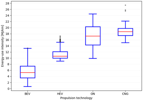
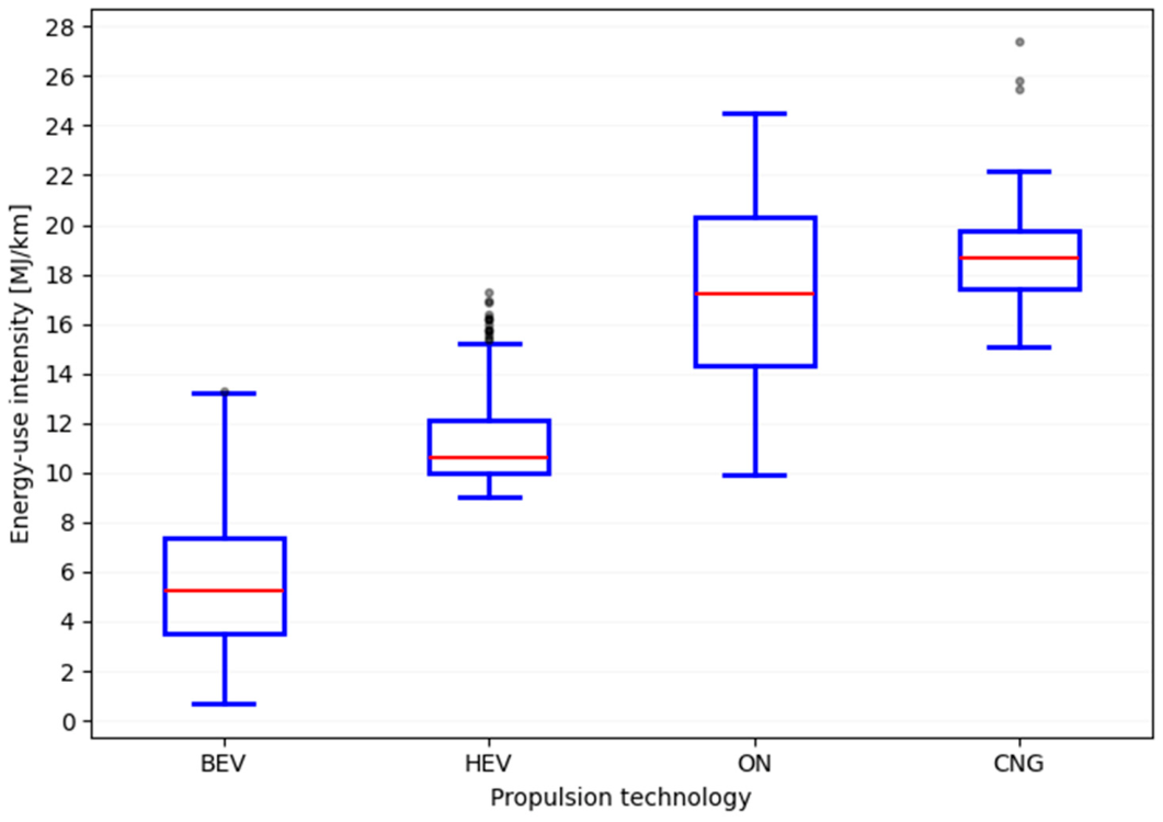
The lowest median energy intensity was observed for BEV (5.24 MJ/km), followed by HEV (10.60 MJ/km), whereas diesel (ON) and CNG showed higher medians (17.21 and 18.63 MJ/km, respectively). The dispersion (IQR) was largest for ON and BEV, indicating higher operational variability in these groups.

A graphical interpretation of the descriptive statistics of the energy-use intensity E/km [MJ/km] by propulsion technology is presented in Figure 1.

3.2. Seasonality

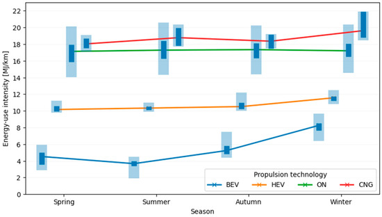
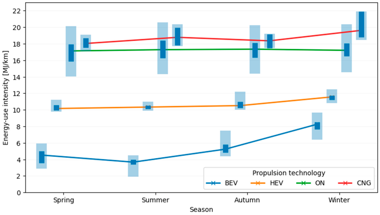
Seasonal variation in energy intensity was analyzed for the technology × season layout using bus-month positional measures (medians and quartiles). The results are presented in

Table 5. Seasonality of energy-use intensity (MJ/km) by technology (median with Q1–Q3).

Season	ON	HEV	BEV	CNG
Winter	17.21 (14.56–20.40)	11.56 (10.81–12.49)	8.27 (6.41–9.86)	19.62 (18.47–21.93)
Spring	17.13 (14.01–20.10)	10.16 (9.78–11.24)	4.52 (2.85–5.91)	18.03 (17.07–19.11)
Summer	17.28 (14.30–20.57)	10.33 (9.91–11.00)	3.67 (1.90–4.48)	18.78 (17.71–20.35)
Autumn	17.34 (14.40–20.27)	10.51 (10.03–12.17)	5.23 (4.38–7.48)	18.36 (17.48–19.22)

Note: Winter (Dec–Feb), Spring (Mar–May), Summer (Jun–Aug), Autumn (Sep–Nov).

. The strongest seasonality was observed for BEV: the median reached 8.27 MJ/km in winter and 3.67 MJ/km in summer, that is, more than a twofold winter penalty in descriptive terms. HEV and CNG also exhibited higher winter values than most other seasons, but CNG showed a higher summer median than spring (18.78 vs. 18.03 MJ/km). Because the CNG subgroup contains only eight buses and 80 bus-months, this pattern should not be interpreted as a stable climatic effect. A plausible operational explanation is that summer CNG duties may have involved different route allocations, higher auxiliary or air-conditioning demand, and/or a small number of high-intensity bus-months; these mechanisms require route-level and auxiliary-consumption data to verify.

Figure 2 presents the distributions of E/km in the technology × season layout (median, IQR, and 95% CI), highlighting the strongest seasonality for BEV and relatively stable values for ON and CNG.

3.3. Mixed-Effects Model: Fixed Effects, Random Effects, and LRT

Associations between propulsion technology and energy intensity were estimated using a linear mixed-effects model with fixed effects for propulsion technology, season, and monthly mileage (log-transformed), and vehicle-level random intercept. For interpretability, the results (

Table 6. (A) Linear mixed-effects model results for log-transformed E/km (fixed effects). (B) Variance components in the mixed-effects model. (C) Likelihood ratio test (LRT) for propulsion-technology effect (ML estimation).

(A)
Variable	Estimate	SE	CI95_Low	CI95_High	p_Value
Intercept	3.9022	0.0928	3.7203	4.0841	<0.001
Technology: CNG vs. ON	0.1392	0.0772	−0.0122	0.2906	0.072
Technology: BEV vs. ON	−1.3032	0.0432	−1.3879	−1.2185	<0.001
Technology: HEV vs. ON	−0.3844	0.048	−0.4785	−0.2903	<0.001
Season: Winter vs. Autumn	0.0594	0.0088	0.0422	0.0766	<0.001
Season: Spring vs. Autumn	−0.0582	0.0087	−0.0752	−0.0411	<0.001
Season: Summer vs. Autumn	−0.0671	0.0088	−0.0842	−0.0499	<0.001
log(distance_km)	−0.1219	0.0105	−0.1426	−0.1013	<0.001
(B)
Component			Variance
Var(bus_id intercept)			0.043
Var(residual)			0.0276
(C)
Test	LRT		df		p-Value
LRT (technology included)	387.259		3		<0.001

) were also discussed in terms of the predicted values for a typical monthly mileage (median distance).

Relative to the diesel reference category (ON), BEV and HEV exhibited significantly lower energy intensities (consistent with large negative fixed coefficients). For CNG, the estimated direction suggested higher values than ON, but the association was not statistically significant at the 0.05 level. Seasonal effects indicated higher energy intensity in winter than in autumn and lower values in spring and summer than in autumn. The mileage term was negative, implying a lower expected MJ/km with a higher monthly distance, although this pattern may also reflect scheduling or route-allocation differences.

To clarify the interpretation of the negative monthly mileage coefficient, the monthly mileage was additionally decomposed into within-bus and between-bus components in pairwise models comparing each alternative technology with diesel (ON). In all three comparisons (BEV vs. ON, HEV vs. ON, and CNG vs. ON), both components were negative and statistically significant; however, the between-bus component was consistently much larger in magnitude than the within-bus component. For example, in the BEV vs. ON comparison, the within-bus coefficient was −0.054, whereas the between-bus coefficient was −0.381; analogous patterns were observed for HEV vs. ON (−0.051 vs. −0.323) and CNG vs. ON (−0.057 vs. −0.313). This indicates that, although a given bus tends to exhibit slightly lower MJ/km in months when it operates more kilometres than its average, the stronger pattern is that buses with systematically higher typical monthly mileages also have systematically lower MJ/km. Therefore, the negative mileage association observed in the main model reflects not only the within-vehicle activity effects but also the between-vehicle allocation and duty cycle differences.

In the Appendix A,

Table A3. Within–between-bus decomposition of the monthly mileage.

Comparison	Variable	Estimate	SE	CI95_Low	CI95_High	p_Value
BEV vs. ON	Within-bus	−0.054	0.013	−0.078	−0.029	0.000019
BEV vs. ON	Between-bus	−0.381	0.047	−0.473	−0.288	5.49 × 10−16
HEV vs. ON	Within-bus	−0.051	0.004	−0.058	−0.044	2.32 × 10−43
HEV vs. ON	Between-bus	−0.323	0.039	−0.400	−0.246	2.04 × 10−16
CNG vs. ON	Within-bus	−0.057	0.004	−0.064	−0.049	9.41 × 10−48
CNG vs. ON	Between-bus	−0.313	0.041	−0.392	−0.233	1.33 × 10−14

presents the within–between decomposition of monthly mileage.

Variance decomposition from the mixed-effects model separates variability due to persistent between-vehicle differences from residual (short-term fluctuations and measurement errors).

Using these components, the intra-class correlation coefficient (ICC)—defined as the share of total variance attributable to between-vehicle differences—was approximately 0.61, indicating that approximately 61% of the remaining variability (after controlling for technology, season, and mileage) can be attributed to systematic differences between buses. In practical MRV applications, estimated random intercepts can therefore support the identification of vehicles with persistently elevated or reduced MJ/km relative to the typical level for their technology.

A likelihood ratio test (LRT) showed that including propulsion technology significantly improved the model fit versus a reduced model without the technology term, confirming that technology is a statistically meaningful source of variation in the observed energy intensity within the analyzed MRV dataset.

3.4. Post hoc Comparisons: Pairwise Technology Differences

Post hoc pairwise comparisons provide a direct assessment of which technologies differ after accounting for other model controls (season and mileage) and averaging the random effects. The results (

Table 7. Post hoc pairwise comparisons for E/km based on the mixed-effects model.

Pair	Ratio (95% CI)	% Difference (95% CI)	p_adj_Holm
BEV vs. ON	0.272 (0.250–0.296)	−72.8% (−75.0% to −70.4%)	<0.001
BEV vs. HEV	0.407 (0.354–0.450)	−60.1% (−64.6% to −55.0%)	<0.001
BEV vs. CNG	0.236 (0.200–0.280)	−76.4% (−80.0% to −72.0%)	<0.001
HEV vs. ON	0.681 (0.620–0.748)	−31.9% (−38.0% to −25.2%)	<0.001
HEV vs. CNG	0.592 (0.498–0.704)	−40.8% (−50.2% to −29.6%)	<0.001
CNG vs. ON	1.149 (0.988–1.337)	14.9% (−1.2% to 33.7%)	0.072

) are expressed as ratios of adjusted mean E/km values, facilitating relative interpretation (values > 1 indicate higher E/km for technology A vs. B; values < 1 indicate lower E/km). p-values were adjusted using the Holm’s method.

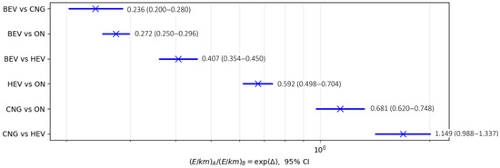
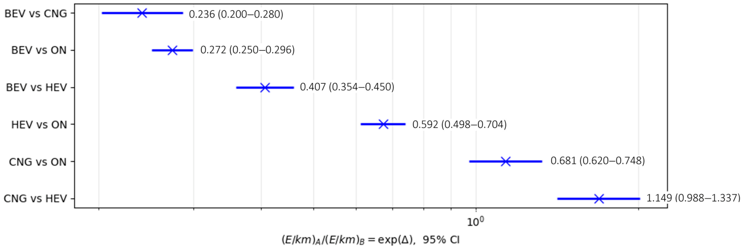
All comparisons involving BEV and HEV (relative to ON and CNG) were statistically significant. The CNG vs. ON contrast was the only non-significant comparison after Holm adjustment (ratio 1.149; p = 0.072). This result should be interpreted as an inconclusive difference rather than evidence of equivalence, because the CNG subgroup was the smallest in the dataset (eight buses; 80 bus-months) and therefore had limited statistical power.

Figure 3 presents the results of the pairwise technology comparisons (post hoc analysis) for the E/km indicator. For each pair, the ratio (E/km)_A/(E/km)_B is reported, which is calculated as the exponent of the difference in fixed effects on the logarithmic scale. Consequently, values greater than one indicate a higher E/km for technology A relative to B, whereas values lower than one indicate a lower E/km for technology A compared with B.

The main BEV vs. ON and HEV vs. ON technology contrasts were robust to balanced subsampling of the dominant diesel group. Across repeated matched-bus samples, the BEV vs. ON and HEV vs. ON ratios remained below one in all runs, and their median values were close to the estimates obtained from the full sample. For CNG vs. ON, however, the resampling results were mixed: only 50.2% of runs yielded p < 0.05 and 1.6% of runs had a ratio below one. Thus, the robustness analysis supports a directional tendency toward higher CNG MJ/km but not a strong inferential conclusion; the possibility of Type II error remains.

In the Appendix A,

Table A4. Robustness analysis for technology-sample imbalance based on balanced subsampling.

Comparison	Main Model Ratio	Median Ratio (500 Resamples)	2.5th Percentile	97.5th Percentile	% of Runs with Ratio < 1	% of Runs with p < 0.05
BEV vs. ON	0.274	0.272	0.254	0.289	100.0	100.0
HEV vs. ON	0.670	0.670	0.623	0.726	100.0	100.0
CNG vs. ON	1.126	1.145	1.009	1.293	1.6	50.2

presents the robustness analysis for technology-sample imbalance based on balanced subsampling.

3.5. Selected EF 3.1 Impact Categories Under WTW

Table 8. EF 3.1 impacts per 1 km by propulsion technology and electricity-mix scenario (WTW).

Scenario/Technology	Climate Change	Particulate Matter	Ionizing Radiation	Photochemical Ozone Formation	Resource Use, Fossils	Water Use
	(kg CO2 eq)	(Disease inc.)	(kBq U-235 eq)	(kg NMVOC eq)	(MJ)	(m3 depriv.)
CNG EURO6	1.036	5.14 × 10−9	1.21 × 10−3	2.09 × 10−3	17.988	0.008
ON EURO5 EEV	1.870	2.20 × 10−8	8.73 × 10−3	5.88 × 10−3	23.949	0.022
ON EURO6	1.520	1.45 × 10−8	7.09 × 10−3	3.56 × 10−3	19.442	0.018
HEV EURO6	1.053	1.09 × 10−8	4.91 × 10−3	2.61 × 10−3	13.468	0.012
BEV mix 2024	0.940	8.39 × 10−9	5.99 × 10−3	2.02 × 10−3	10.597	0.091
BEV mix 2030	0.521	6.56 × 10−9	7.11 × 10−3	1.19 × 10−3	6.203	0.066
BEV mix 2040	0.127	4.89 × 10−9	1.62 × 10−1	4.13 × 10−4	4.748	0.032
BEV mix 2050	0.066	4.95 × 10−9	1.92 × 10−1	3.12 × 10−4	4.595	0.024

reports per-kilometre impacts in selected EF 3.1 categories under well-to-wheel (WTW) boundaries by propulsion technology. The results are shown for Poland’s 2024 electricity mix and electricity-mix scenarios for 2030, 2040, and 2050. Calculations were based on the annual energy/fuel use per kilometre estimated for the PKM Katowice fleet.

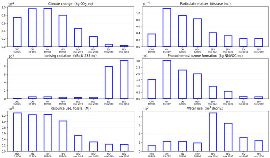
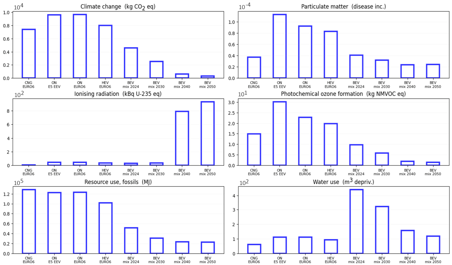
Emission values in selected EF 3.1 impact categories, calculated for a typical bus-month by propulsion technology, considering EURO emission standards and Poland’s electricity-generation mix in 2024 and projections for 2030, 2040, and 2050. Bus bus-month results (Figure 4) were computed as follows: EF_per-km (Table 8) × median monthly mileage for a given technology (Table 1).

Annual fleet-level impacts were derived from (i) per-kilometre indicators and (ii) annual mileages by technology group. Per-kilometre values were computed using a km-weighted average energy/fuel intensity in 2024 (total carrier consumption divided by total distance within each technology), and annual totals were obtained by multiplying the per-km values by the annual mileage. The results are summarized in

Table 9. Annual totals of selected EF 3.1 categories for the analyzed fleet by propulsion technology (WTW), with electricity-mix scenarios through 2050.

Scenario/Technology	Climate Change	Particulate Matter	Ionizing Radiation	Photochemical Ozone Formation	Resource Use, Fossils	Water Use
	(kg CO2 eq)	(Disease inc.)	(kBq U-235 eq)	(kg NMVOC eq)	(MJ)	(m3 depriv.)
CNG EURO 6	6.07 × 105	3.01 × 10−3	7.11 × 102	1.22 × 103	1.05 × 107	4.97 × 103
ON EURO5 EEV	6.72 × 106	7.92 × 10−2	3.14 × 104	2.11 × 104	8.60 × 107	7.77 × 104
ON EURO 6	1.51 × 107	1.43 × 10−1	7.03 × 104	3.53 × 104	1.93 × 108	1.74 × 105
HEV EURO 6	2.08 × 106	2.17 × 10−2	9.72 × 103	5.17 × 103	2.67 × 107	2.41 × 104
BEV mix 2024	1.45 × 106	1.30 × 10−2	9.26 × 103	3.12 × 103	1.64 × 107	1.40 × 105
BEV mix 2030	8.04 × 105	1.01 × 10−2	1.10 × 104	1.84 × 103	9.58 × 106	1.02 × 105
BEV mix 2040	1.95 × 105	7.55 × 10−3	2.50 × 105	6.38 × 102	7.33 × 106	4.97 × 104
BEV mix 2050	1.02 × 105	7.65 × 10−3	2.96 × 105	4.82 × 102	7.10 × 106	3.73 × 104

.

3.6. Illustrative Traffic-Management Screening Analysis

An illustrative traffic-management screening scenario analysis was conducted to show how assumed changes in operational energy intensity could be translated into EF 3.1 results within the adopted WTW boundary. Three operational improvement variants were assumed, modelled as 3%, 5%, and 10% reductions in propulsion energy intensity (E/km) relative to the baseline. These values are treated here as screening parameters inspired by the ITS and transit-priority literature, not as effects empirically identified for the studied fleet through before–after observations, traffic simulations, or quasi-experimental methods.

The 3% variant represents a conservative scenario, the 5% variant an intermediate scenario, and the 10% variant an upper but still illustrative case based on values reported in the ITS and eco-driving literature [27,28,29]. The adopted percentages are intended only to illustrate how the MRV/WTW framework responds to plausible improvements in bus trajectory smoothness, given the established relationship between stop frequency and increased fuel use or emissions [7], and the broader ITS literature on reducing congestion and stop-and-go dynamics [30]. For comparability, identical reduction levels were applied across propulsion technologies, although real-world effects may vary by corridor, season, propulsion technology, passenger load, and driver behaviour [31].

Within the WTW system boundaries adopted in this study, inventory flows (WTT/TTW) are treated as linearly proportional to energy/fuel consumption; therefore, a proportional reduction in E/km implies the same proportional reduction across the reported EF 3.1 categories, and absolute reductions are scaled with the 2024 baseline totals.

Table 10. Absolute reductions in selected EF 3.1 impacts relative to the 2024 baseline under E/km reduction scenarios.

Scenario/Technology	Climate Change	Particulate Matter	Ionizing Radiation	Photochemical Ozone Formation	Resource Use, Fossils	Water Use
	(kg CO2 eq)	(Disease inc.)	(kBq U-235 eq)	(kg NMVOC eq)	(MJ)	(m3 depriv.)
3%	7.781 × 105	7.808 × 10−3	3.640 × 10−3	1.886 × 10−3	9.975 × 10−6	1.263 × 10−4
5%	1.297 × 10−6	1.301 × 10−2	6.067 × 10−3	3.143 × 10−3	1.663 × 10−7	2.105 × 10−4
10%	2.594 × 10−6	2.603 × 10−2	1.213 × 10−4	6.287 × 10−3	3.325 × 10−7	4.210 × 10−4

reports the absolute reductions for all three variants.

Under the linearity assumption, the 3%, 5%, and 10% variants reduce the baseline impacts by exactly 3%, 5%, and 10%, respectively; equivalently, the remaining values are 97%, 95%, and 90% of the 2024 baseline. For the fleet’s total annual impacts in 2024, this corresponds, for example, to a reduction in climate change of approximately 0.78/1.30/2.59-million-kilogram CO₂ eq, and in resource use, fossils of approximately 10.0/16.6/33.3 million MJ.

This scenario analysis was purely indicative and should be read as preliminary screening rather than evidence of the effect of a specific traffic-management intervention. It is useful for prioritization because it shows the order of magnitude of possible benefits if corridor or intersection measures succeed in reducing E/km. In practice, such effects may differ by corridor, line, season, powertrain, passenger load, and traffic state, and exhaust emissions may respond nonlinearly to changes in speed profiles and stopping patterns. A more rigorous evaluation would require route-level traffic-dynamics data, before–after observations, and controlled or simulation-based modelling.

4. Discussion

The obtained results allow us to address H1–H4 and the application question concerning the order of magnitude of WTW benefits under the assumed reductions in E/km. In this section, we interpret the findings in the context of prior evidence and discuss their implications for fleet management, smart mobility monitoring, and preliminary screening of traffic-management measures.

4.1. Technological Differences in MJ/km and Their Interpretation

The mixed-effects model shows that propulsion technology is the strongest observed explanatory factor in the fitted model, with BEV and HEV buses achieving significantly lower MJ/km values than diesel buses. The direction and magnitude of these associations are consistent with comparative studies of urban bus powertrains, which explain the advantage of electric and hybrid drivetrains by their higher efficiency and regenerative braking under stop-and-go driving profiles [32,33,34].

For CNG, the results do not support a strong claim of lower operational energy intensity relative to diesel. The point estimate is slightly higher than ON, but the CNG fleet is small and the confidence interval overlaps diesel. Policy interpretation should therefore be cautious: CNG may still have specific local-air-quality or transitional fleet-management roles under certain WTT/TTW assumptions, but the present MRV evidence does not demonstrate an energy-efficiency advantage over diesel in this fleet. Decisions on CNG deployment should be based on multi-criteria evidence, including pollutant emissions, infrastructure, methane leakage risk, fuel prices, and local operating conditions [35,36].

The within–between decomposition provides a more cautious interpretation of the mileage effect than the main model. The fact that the between-bus component is substantially stronger than the within-bus component suggests that the negative coefficient on log (monthly mileage) should not be interpreted purely as evidence that higher mileage improves energy efficiency. Rather, it appears to capture, to a considerable extent, the differences in vehicle assignment, duty cycles, and types of services typically performed by different buses. Simultaneously, the smaller but significant within-bus component indicates that months with above-average activity for the same vehicle are also associated with slightly lower MJ/km values. Accordingly, the mileage term should be understood primarily as an activity and allocation control, rather than as a direct efficiency parameter. This interpretation is more consistent with the operational nature of fleet data and helps reduce the risk of overinterpreting the mileage effect as an intrinsic technological advantage. However, because the detailed route and traffic dynamics variables are not observed here, this coefficient should be interpreted cautiously rather than as a pure efficiency effect [37,38].

4.2. Seasonality and Winter Penalty, Particularly for BEV

Seasonality is confirmed both in the descriptive analysis and in the model: energy-use intensity increases in winter, and the effect is strongest for BEV. In descriptive terms, the BEV median more than doubled between summer and winter. Plausible mechanisms include reduced battery and drivetrain efficiency at low temperatures, higher heating and defrosting auxiliary loads, preconditioning and thermal-management demand, and winter service conditions that may increase dwell time, rolling resistance, and stop-and-go operation [39]. Because the present dataset does not directly observe temperature, auxiliary/traction energy split, or traffic dynamics, these mechanisms should be interpreted as plausible contextual explanations rather than identified causal drivers. The annual BEV ratio of 0.272 is therefore most directly applicable to metropolitan fleets with climatic and operational conditions comparable to the 2024 Polish case; direct extrapolation to substantially milder or more severe winter climates should be avoided [40,41].

4.3. Between-Vehicle Heterogeneity and the Role of MRV

The high share of variance attributed to between-bus differences (ICC) indicates that, even after accounting for technology, season, and activity level, persistent vehicle-specific differences remain within the MRV framework. In practical MRV applications, estimated random intercepts can flag positive anomalies (buses with persistently lower MJ/km than expected for the same technology, season, and mileage) and negative anomalies (persistent excess MJ/km potentially associated with technical faults, battery degradation, auxiliary loads, route assignment, or driver behaviour). However, bus-month data alone do not contain enough information to diagnose the source of a deviation. Root-cause MRV would require second-by-second CAN-bus/AVL data, state-of-charge information for BEV, passenger-load data, route context, and maintenance records.

The technical characteristics summarized in Table A1 also indicate a natural extension of the model. Vehicle age in 2024 can be calculated as 2024 minus the year of manufacture; however, it was not included in the main specification because age, EURO standard, and propulsion technology are strongly collinear in this fleet. For example, the BEV and HEV groups are concentrated in newer cohorts, whereas part of the diesel fleet consists of older EURO V/EEV vehicles. A larger multi-operator dataset or a longer time series could include age as a fixed effect, nonlinear term, or random slope to separate ageing from technology and assignment effects.

4.4. WTW EF 3.1 Results: Electricity Mix and Multi-Criteria Trade-Offs

The WTW assessment (EF 3.1) confirms that BEV climate benefits depend on the electricity generation mix: as the grid decarbonizes, the reduction in the climate change category increases, consistent with LCA findings for electric buses [42,43]. Simultaneously, the multi-criteria analysis reveals potential trade-offs in categories linked to generation technologies, for example, an increase in ionizing radiation under higher nuclear shares, reflecting updated characterization factors and upstream profiles [44].

It should be emphasized that these results are bounded by use-phase WTW system boundaries. They include energy-carrier production and delivery (WTT) and vehicle operation/tailpipe emissions (TTW), but they exclude vehicle manufacturing, battery production and replacement, charging or refuelling infrastructure, depot infrastructure, and maintenance. Consequently, BEV results should be interpreted as operational WTW comparisons rather than complete life-cycle environmental superiority claims. Prior work indicates that extending the boundaries to a full life-cycle perspective may shift the burdens between manufacturing and operation, particularly for BEV buses [42,43].

Electricity mix scenarios for 2030–2050 should be interpreted as illustrative variants used for sensitivity analysis rather than deterministic forecasts. The actual development pathway of the electricity mix depends on public policies, investment decisions, and macroeconomic conditions. Therefore, the EF 3.1 results for future years should be understood as being sensitive to the assumed electricity mix rather than as fixed or certain impact values.

4.5. Traffic-Management Relevance and the Role of MRV Indicators

Research on urban traffic shows that congestion and intersection stops generate substantial excess fuel consumption and emissions [30,45]. Studies on public-transport priority also point to the possibility of reducing delay and energy use, although the effects depend on traffic conditions and how priority is balanced across competing streams [9,27,46].

In the present illustrative traffic-management screening exercise, the assumed 3–10% reductions in E/km were treated as scenario parameters rather than empirically identified ITS effects; within the adopted WTW boundary, they implied proportional reductions in LCIA results. This framing is useful for rapid screening of the potential scale of benefits, but it does not replace empirical or simulation-based evaluations built on traffic-dynamics data and instantaneous emission models. This distinction is important because exhaust-emission responses of diesel, CNG, and hybrid buses may be nonlinear under stop-and-go profiles, whereas average-speed COPERT/EMEP factors are adequate for fleet-level screening but not for microscopic intervention evaluation [47,48,49].

From a sustainable road design perspective, the present results are most relevant for monitoring contexts in which intersection and corridor measures are expected to reduce stops and smooth bus trajectories at bottlenecks. Therefore, the proposed MRV indicators (MJ/km and EF 3.1 WTW) can be treated as candidate before–after KPIs for measures such as transit signal priority (TSP), coordinated/adaptive signal control, or corridor-level prioritization, provided that route- or corridor-level implementation data are available. A logical next step after integration with AVL/GPS and traffic-quality measures would be to enable intersection- or corridor-level assessment of how geometry and control are associated with energy use and environmental impacts.

4.6. Limitations and Directions for Future Research

The main limitations arise from the scope and granularity of the data. The dataset does not contain route characteristics, stop density, intersection frequency, congestion, average speed, passenger load, topography, ambient temperature, detailed speed profiles, auxiliary/traction energy split, or driver behaviour. Because these operational covariates were unavailable, the estimated propulsion effects may partly absorb route- and service-assignment differences and should be interpreted as reduced-form associations. Accordingly, the technology coefficients are adjusted associations within the available MRV dataset, not causal effects isolated from operating conditions. Vehicle age was derivable from Table A1 but was not estimated in the current single-operator model because of strong collinearity with propulsion technology and EURO standard; therefore, no inference on ageing effects can be drawn from the present dataset. A second limitation is the emission-modelling approach: TTW factors were assigned using a macroscopic average-speed COPERT/EMEP-EEA logic, which does not represent second-by-second acceleration, idling, regenerative braking, or transient combustion in urban stop-and-go service and may bias HEV and CNG comparisons. Third, the WTW boundary excludes vehicle manufacturing, batteries, charging/refuelling infrastructure, depot infrastructure, and maintenance, so the EF 3.1 results are not a full LCA. Fourth, the CNG sample is small (eight buses and 80 bus-months), increasing uncertainty and the risk of Type II error. Future work should integrate MRV with AVL/GPS, CAN-bus and passenger-counting data; estimate corridor/intersection effects using before–after, quasi-experimental or microsimulation designs; separate BEV auxiliary and traction demand; and extend the environmental assessment to full life-cycle inventories.

5. Conclusions

Conclusions were formulated based on the MRV data for the bus fleet, together with the mixed-effects results and WTW assessment (EF 3.1). The key findings and their implications for smart urban mobility are as follows.

• Propulsion technology is significantly associated with energy-use intensity. Relative to diesel (ON), clearly lower MJ/km was estimated for BEV (ratio 0.272) and HEV (ratio 0.681), indicating that electrification and hybridization are associated with higher operational energy efficiency in urban services. The CNG point estimate was higher than diesel, but the result was not statistically conclusive; it should not be read as evidence of equivalence or as a demonstrated energy-efficiency disadvantage under the available small CNG sample.
• Seasonality is critical for operational planning, especially for BEV. The descriptive BEV median more than doubled in winter compared with summer, so range planning, charging strategies, and cross-technology comparisons should explicitly account for heating and thermal-management demand. The annual BEV advantage should be interpreted in the climatic and operational context of the 2024 Polish metropolitan fleet.
• A large share of MJ/km variability was vehicle-specific (high ICC), even after accounting for technology, season, and activity level within the available MRV dataset. This supports MRV at the vehicle level and can help distinguish positive and negative performance anomalies for further investigation; however, monthly totals alone cannot identify whether a deviation is technical, operational, or behavioural. CAN-bus/AVL, passenger-load, and maintenance data are needed for root-cause diagnosis.
• In the WTW assessment (EF 3.1), BEV shows a favourable climate profile within the adopted operational WTW boundary, and the advantage increases with electricity-mix decarbonization. However, the boundary excludes vehicle manufacturing, batteries, charging infrastructure, depot infrastructure, and maintenance, and the multi-criteria results indicate potential trade-offs (e.g., ionizing radiation and water use) that depend on the generation technologies represented in the mix.
• The illustrative traffic-management scenarios showed that if E/km were reduced by 3–10%, proportional reductions in WTW impacts would follow within the adopted system boundary. These are screening assumptions, not empirically measured ITS effects. In practice, the magnitude of such benefits depends on corridor characteristics, seasonality, propulsion technology, passenger load, traffic state, and the share of auxiliary consumption in BEV. Further research should link MRV with trajectory and traffic-dynamics data, apply before–after or quasi-experimental ITS evaluation, and extend the environmental assessment to full vehicle and infrastructure life cycles.

Therefore, the main contribution of this study is methodological and practical: it provides a repeatable workflow for monitoring, benchmarking, and preliminary screening in a smart city transport context, rather than a direct causal evaluation of smart-road interventions.

References

- Bıyık, C.; Abareshi, A.; Paz, A.; Ruiz, R.A.; Battarra, R.; Rogers, C.D.F.; Lizarraga, C. Smart Mobility Adoption: A Review of the Literature. J. Open Innov. Technol. Mark. Complex. 2021, 7, 146. [Google Scholar] [CrossRef] [Scilit]
- Banister, D. The Sustainable Mobility Paradigm. Transp. Policy 2008, 15, 73–80. [Google Scholar] [CrossRef] [Scilit]
- Tirachini, A.; Godachevich, J.; Cats, O.; Muñoz, J.C.; Soza-Parra, J. Headway Variability in Public Transport: A Review of Metrics, Determinants, Effects for Quality of Service and Control Strategies. Transp. Rev. 2022, 42, 337–361. [Google Scholar] [CrossRef] [Scilit]
- Ibarra-Rojas, O.J.; Delgado, F.; Giesen, R.; Muñoz, J.C. Planning, Operation, and Control of Bus Transport Systems: A Literature Review. Transp. Res. Part B Methodol. 2015, 77, 38–75. [Google Scholar] [CrossRef] [Scilit]
- Hosking, J.; Braubach, M.; Buss, D.; Khayesi, M.; Pavarino Filho, V.; de Sá, T.H. Towards a Global Framework for Transport, Health and Health Equity. Environ. Int. 2022, 169, 107472. [Google Scholar] [CrossRef] [Scilit] [PubMed]
- Ricardo Energy & Environment. Study on the Deployment of C-ITS in Europe Final Report; TRT: London, UK, 2016. [Google Scholar]
- Rakha, H.; Ding, Y. Impact of Stops on Vehicle Fuel Consumption and Emissions. J. Transp. Eng. 2003, 129, 23–32. [Google Scholar] [CrossRef] [Scilit]
- Song, G.; Zhou, X.; Yu, L. Delay Correction Model for Estimating Bus Emissions at Signalized Intersections Based on Vehicle Specific Power Distributions. Sci. Total Environ. 2015, 514, 108–118. [Google Scholar] [CrossRef] [Scilit]
- Liu, H.; Zhang, Y.; Zhang, K. Evaluating Impacts of Intelligent Transit Priority on Intersection Energy and Emissions. Transp. Res. Part D Transp. Environ. 2020, 86, 102416. [Google Scholar] [CrossRef] [Scilit]
- ISO 14040:2006; Environmental Management—Life Cycle Assessment—Principles and Framework. International Organization for Standardization: Geneva, Switzerland, 2006. Available online: https://www.iso.org/standard/37456.html (accessed on 25 February 2026).
- Greenhouse Gas Protocol. Policy and Action Standard Road Transport Sector Guidance; World Resources Institute: Washington, DC, USA, 2015. [Google Scholar]
- MobiliseYourCity Secretariat. Monitoring & Reporting Approach for GHG Emissions; MobiliseYourCity Secretariat: Brussels, Belgium, 2020. [Google Scholar]
- Eichhorst, U.; Bongardt, D.; Novikova, V. Compendium on Greenhouse Gas Baselines and Monitoring Passenger and Freight Transport, 2nd ed.; UNFCCC: Bonn, Germany, 2018. [Google Scholar]
- Budimir, D.; Jelušić, N.; Perić, M. Floating Car Data Technology. Sci. J. Marit. Res. 2019, 33, 22–32. [Google Scholar] [CrossRef] [Scilit]
- Barlow, T.J.; Boulter, P.G. Emission Factors 2009 Report 2—A Review of the Average-Speed Approach for Estimating Hot Exhaust Emissions; TRL Limited: Wokingham, UK, 2009. [Google Scholar]
- Tsanakas, N.; Ekstrom, J.; Olstam, J. Estimating Emissions from Static Traffic Models Problems and Solutions. J. Adv. Transp. 2020, 2020, 5401792. [Google Scholar] [CrossRef] [Scilit]
- Lee, E.H. eXplainable DEA Approach for Evaluating Performance of Public Transport Origin-Destination Pairs. Res. Transp. Econ. 2024, 108, 101491. [Google Scholar] [CrossRef] [Scilit]
- Manandhar, B.; Dunkel Vance, K.; Rawat, D.B.; Yilmaz, N. Leveraging Digital Twin Technology for Sustainable and Efficient Public Transportation. Appl. Sci. 2025, 15, 2942. [Google Scholar] [CrossRef] [Scilit]
- Liu, Z.; Chen, H.; Liu, E.; Zhang, Q. Evaluating the Dynamic Resilience of the Multi-Mode Public Transit Network for Sustainable Transport. J. Clean. Prod. 2022, 348, 131350. [Google Scholar] [CrossRef] [Scilit]
- Liu, Z.; Sun, D.J.; Chen, H.; Hao, W.; Wang, Z.; Tang, F. Resilience-Based Post-Disaster Repair Strategy for Integrated Public Transit Networks. Transp. B Transp. Dyn. 2024, 12, 1–25. [Google Scholar] [CrossRef] [Scilit]
- Cooney, G.; Hawkins, T.R.; Marriott, J. Life Cycle Assessment of Diesel and Electric Public Transportation Buses. J. Ind. Ecol. 2013, 17, 689–699. [Google Scholar] [CrossRef] [Scilit]
- Intergovernmental Panel on Climate Change (IPCC). 2006 IPCC Guidelines for National Greenhouse Gas Inventories. Volume 2: Energy; IGES: Hayama, Japan, 2006; Available online: https://www.ipcc-nggip.iges.or.jp/public/2006gl/vol2.html (accessed on 8 April 2026).
- National Institute of Standards and Technology (NIST). Guide to the SI, Appendix B: Conversion Factors; NIST: Gaithersburg, MD, USA, 2016; Available online: https://www.nist.gov/pml/special-publication-811/nist-guide-si-appendix-b-conversion-factors (accessed on 8 April 2026).
- GAZ-SYSTEM S.A. NTS Gaseous Fuel Quality Specifications; GAZ-SYSTEM S.A.: Warsaw, Poland, 2023; Available online: https://www.gaz-system.pl/en/for-customers/services-in-the-nts/nts-gas-quality-specifications.html (accessed on 9 April 2026).
- U.S. Department of Energy, Alternative Fuels Data Center. Fuel Properties Comparison; U.S. Department of Energy: Washington, DC, USA, 2026; Available online: https://www.gaz-system.pl/en/for-customers/services-in-the-nts/nts-gas-quality-specifications.html (accessed on 9 April 2026).
- European Commission Joint Research Centre COPERT. Computer Model to Calculate Emissions from Road Traffic; European Commission, Joint Research Centre: Ispra, Italy, 2026. [Google Scholar]
- Abbasi, M.; Hosseinlou, M.H.; Sarreshtehdari, A.; Mandzuka, S. Evaluation of Transit Signal Priority for Bus Rapid Transit in Heterogeneous Traffic Flow. Teh. Vjesn. 2021, 28, 2080–2087. [Google Scholar] [CrossRef] [Scilit]
- Shaaban, K.; Ghanim, M. Evaluation of Transit Signal Priority Implementation for Bus Transit along a Major Arterial Using Microsimulation. Procedia Comput. Sci. 2018, 130, 82–89. [Google Scholar] [CrossRef] [Scilit]
- Chen, H.; Rakha, H.A. Developing and Field Testing a Green Light Optimal Speed Advisory System for Buses. Energies 2022, 15, 1491. [Google Scholar] [CrossRef] [Scilit]
- Lv, Z.; Shang, W. Impacts of Intelligent Transportation Systems on Energy Conservation and Emission Reduction of Transport Systems: A Comprehensive Review. Green Technol. Sustain. 2023, 1, 100002. [Google Scholar] [CrossRef] [Scilit]
- Lyu, A.; Zhang, H.; Zhang, Y.; Li, C.; Chen, Y. A Study on Energy Consumption Analysis and Prediction of Electric Bus at Intersections Considering Driving Behavior. Sci. Rep. 2025, 15, 44755. [Google Scholar] [CrossRef] [Scilit] [PubMed]
- Zhang, S.; Wu, Y.; Liu, H.; Huang, R.; Yang, L.; Li, Z.; Fu, L.; Hao, J. Real-World Fuel Consumption and CO2 Emissions of Urban Public Buses in Beijing. Appl. Energy 2014, 113, 1645–1655. [Google Scholar] [CrossRef] [Scilit]
- Kivekas, K.; Lajunen, A.; Vepsalainen, J.; Tammi, K. City Bus Powertrain Comparison Driving Cycle Variation and Passenger Load Sensitivity Analysis. Energies 2018, 11, 1755. [Google Scholar] [CrossRef] [Scilit]
- Zhang, Z.; Ye, B.; Wang, S.; Ma, Y. Analysis and Estimation of Energy Consumption of Electric Buses Using Real-World Data. Transp. Res. Part D Transp. Environ. 2024, 126, 104017. [Google Scholar] [CrossRef] [Scilit]
- Perdikopoulos, M.; Karageorgiou, T.; Ntziachristos, L.; Deville Cavellin, L.; Joly, F.; Vigneron, J.; Arfire, A.; Debert, C.; Sanchez, O.; Gaie-Levrel, F.; et al. Developing Emission Factors from Real-World Emissions of Euro VI Urban Diesel, Diesel-Hybrid, and Compressed Natural Gas Buses. Atmosphere 2025, 16, 293. [Google Scholar] [CrossRef] [Scilit]
- Rosero, F.; Fonseca, N.; López, J.-M.; Casanova, J. Real-World Fuel Efficiency and Emissions from an Urban Diesel Bus Engine under Transient Operating Conditions. Appl. Energy 2020, 261, 114442. [Google Scholar] [CrossRef] [Scilit]
- de Abreu e Silva, J.; Moura, F.; Garcia, B.; Vargas, R. Influential Vectors in Fuel Consumption by an Urban Bus Operator Bus Route, Driver Behavior or Vehicle Type. Transp. Res. Part D Transp. Environ. 2015, 38, 94–104. [Google Scholar] [CrossRef] [Scilit]
- Ma, H.; Xie, H.; Huang, D.; Xiong, S. Effects of Driving Style on the Fuel Consumption of City Buses under Different Road Conditions and Vehicle Masses. Transp. Res. Part D Transp. Environ. 2015, 41, 205–216. [Google Scholar] [CrossRef] [Scilit]
- Gu, J.; Liao, Q.; Zhang, K.M. Assessing the Cold Weather Impact on Battery Electric Transit Buses. Transp. Res. Part D Transp. Environ. 2025, 145, 104809. [Google Scholar] [CrossRef] [Scilit]
- Liu, K.; Wang, J.; Yamamoto, T.; Morikawa, T. Modelling the Multilevel Structure and Mixed Effects of the Factors Influencing the Energy Consumption of Electric Vehicles. Appl. Energy 2016, 183, 1351–1360. [Google Scholar] [CrossRef] [Scilit]
- Espinosa, M.; Márquez, F. Monitoring, Reporting, and Verification Systems for Electric Bus Projects a Methodological Guide to Their Design, Based on a Case Study in Colombia; MobiliseYourCity Secretariat: Brussels, Belgium, 2021. [Google Scholar]
- Nordelof, A.; Romare, M.; Tivander, J. Life Cycle Assessment of City Buses Powered by Electricity, Hydrogenated Vegetable Oil or Diesel. Transp. Res. Part D Transp. Environ. 2019, 75, 211–222. [Google Scholar] [CrossRef] [Scilit]
- Ellingsen, L.A.W.; Thorne, R.J.; Wind, J.; Figenbaum, E.; Romare, M.; Nordelof, A. Life Cycle Assessment of Battery Electric Buses. Transp. Res. Part D Transp. Environ. 2022, 112, 103498. [Google Scholar] [CrossRef] [Scilit]
- Andreasi Bassi, S.; Biganzoli, F.; Ferrara, N.; Amadei, A.; Valente, A.; Sala, S.; Ardente, F. Updated Characterisation and Normalisation Factors for the Environmental Footprint 3.1 Method; JRC130796; Publications Office of the European Union: Luxembourg, 2023. [Google Scholar] [CrossRef]
- Barth, M.; Boriboonsomsin, K. Real-World CO2 Impacts of Traffic Congestion. In Proceedings of the 87th Annual Meeting of the Transportation Research Board, Washington, DC, USA, 13–17 January 2008. [Google Scholar]
- Lin, Y.; Yang, X.; Zou, N.; Franz, M. Transit Signal Priority Control at Signalized Intersections A Comprehensive Review. Transp. Lett. Int. J. Transp. Res. 2015, 7, 168–180. [Google Scholar] [CrossRef] [Scilit]
- Boulter, P.G.; McCrae, I.S.; Barlow, T.J. A Review of Instantaneous Emission Models for Road Vehicles; TRL Limited: Wokingham, UK, 2007. [Google Scholar]
- Franco, V.; Kousoulidou, M.; Muntean, M.; Ntziachristos, L.; Hausberger, S.; Dilara, P. Road Vehicle Emission Factors Development A Review. Atmos. Environ. 2013, 70, 84–97. [Google Scholar] [CrossRef] [Scilit]
- Lejri, D.; Can, A.; Schiper, N.; Leclercq, L. Accounting for Traffic Speed Dynamics When Calculating COPERT and PHEM Pollutant Emissions at the Urban Scale. Transp. Res. Part D Transp. Environ. 2018, 63, 588–603. [Google Scholar] [CrossRef] [Scilit]
Disclaimer/Publisher’s Note: The statements, opinions and data contained in all publications are solely those of the individual author(s) and contributor(s) and not of MDPI and/or the editor(s). MDPI and/or the editor(s) disclaim responsibility for any injury to people or property resulting from any ideas, methods, instructions or products referred to in the content. |
© 2026 by the author. Licensee MDPI, Basel, Switzerland. This article is an open access article distributed under the terms and conditions of the Creative Commons Attribution (CC BY) license.