High-Frequency Infrared Thermography Reveals Short-Term Pressure Variations in CO₂ Natural Vents at Mefite d’Ansanto (Italy)

Abstract

A thermal infrared (TIR) camera was installed at Mefite Lake in Valle d’Ansanto, Irpinia (Italy), to assess whether small variations in cold CO₂ flux can be resolved thermally. To our knowledge, this is the first systematic attempt to extract short-period degassing dynamics from TIR data at Mefite. Infrared thermal images taken over a three-hour nighttime interval revealed the spatial distribution and extent of natural CO₂ emissions. The high sampling frequency of one minute detected unexpected thermal variability from the source. The extent of temperature variations across the entire site reached almost 3 °C, with durations typically ranging from a few minutes to tens of minutes. Spectral analysis of the temperature time series reported a 1/f-type noise pattern, with significant periods of 2–3 min, 5 min, 26 min, and 61 min observed at different locations. Further intermediate periods were observed at individual points. Differences and delays in temperature variations appeared to be related to distance from the structure’s centre and the presence of water. These temperature fluctuations were interpreted as changes in the gaseous emission flow caused by a few kPa of CO₂ escaping due to pressure variations. The gas thermally interacts with the underlying soil, adding or removing heat at the surface. These results demonstrate that high-frequency infrared thermography provides a sensitive and practical tool for quantifying short-term flux variability at natural CO₂ vents and for improving the characterisation of their degassing dynamics.

1. Introduction

Near the Tyrrhenian side of the southern Apennine chain in Italy, Mefite d’Ansanto is a well-known site of cold fluid discharge, considered the most abundant worldwide [1]. The area has been subjected to two broadly contemporaneous events. The first is linked to the build-up of the southern Apennine belt, originating from the deformation of the Adriatic passive margin, which began in the Miocene and continued into the early Pleistocene, in an NE direction [2]. The second event is linked to extensional tectonics that led to the opening of the Tyrrhenian Sea and crustal thinning, dating back to the middle Pleistocene, likely driven, among other factors, by the 2-million-year-old Marsili spreading ridge [3]. Thus, compressive tectonics cooperated synergistically with extensional tectonics trending NE-SW, resulting in normal faults and antiforms with NW-SE-directed axes parallel to the Apennine structure.

Current GNSS and SAR surface interferometry measurements generally indicate that surface displacement is trending NE [4], albeit with some variations. Directed N-NW motion on the Tyrrhenian side was reported with average values of 1–3 mm y⁻¹ [5], while the neighbouring site on the Adriatic side records average values of 4.5–5.5 mm y⁻¹ in the NE direction. These authors suggested that this differential motion causes tension along the Apennines’ crest. One manifestation of these tensions would be the 23 November 1980 Mw 6.9 Irpinia earthquake. The deformation rate observed in the area was hypothesised to be a prerequisite for the occurrence of strong earthquakes [6]. Indeed, observations from the 1980 earthquake, including the identification of a NE-dipping, NW–SE-orientated normal fault, led the authors to conclude that “the high strain rate level indicates that the scenario of a new strong earthquake in Irpinia is not unlikely.”

The Mefite d’Ansanto site, in the context described above, exhibits a bubbling mud lake during autumn to early summer, while it is dry from midsummer until autumn. The gas composition is as follows: CO₂ up to~98% v/v, N₂~1.3% v/v, H₂S~0.33% v/v, CH₄~0.23% v/v [7], H₂ 36 ppm, and He_tot 8 ppm [8,9] with ³He/⁴He ratio (expressed as R/Ra) of 2.72 [1]. CO₂ total discharge was estimated at around 2000 tons per day, equal to approximately 730,000 tons per year from a rough area of 4000 m². In other words, 7.3 × 10¹¹ g y⁻¹, about 2.32 kg s⁻¹. That means a yearly flux of 5.8 × 10⁻³ kg s⁻¹ m⁻², indicating high permeability associated with mantle sources. For comparison, consider that 5.6 × 10⁻⁹ kg s⁻¹ m⁻² were measured in the Mount Vulture volcanic area [10]. Elsewhere in a compressional tectonic regime, but still with documented mantle contribution (i.e., helium isotope data), CO₂ flux values from 2.5 × 10⁻¹² to 1.1 × 10⁻¹¹ kg s⁻¹ m⁻² were measured [11]. In the Monte Amiata area, instead, 13,350 tons day⁻¹ over an average area of 225 km², i.e., 6.9 × 10⁻⁷ kg s⁻¹ m⁻², were reported [12]. These comparative values evidence that the highest flux values exist at Mefite d’Ansanto, which, according to some authors [13,14], could also be due to the continuous supply derived from the subducted Adria slab.

Gas emissions at the Mefite site show significant temporal variability, noticeable to attentive visitors through sudden intensifications or reductions in acoustic noise. Historically, some local inhabitants reported large variations in acoustic noise during disastrous seismic events. Thus, the FURTHER project recently examined the role of fluids during the preparatory phase of earthquakes in this region, revealing non-steady behaviour of the Mefite emissions. It was based on acoustic spectral analyses [15] and on seismic tremors in the 3–20 Hz range [16]. However, such methodologies fail to quantify the amplitudes of flux variations, and a direct sampling by large funnels would be required. Moreover, direct sampling is difficult due to the pool size, the irregular surface with mud, and high CO₂ concentrations. Therefore, the question arises as to whether the observed variations could also occur in the infrared spectrum. In fact, the discharged gases always have a slightly different temperature from the atmosphere, exchanging heat with the ground surface depending on the flow velocity.

Remote sensing for thermal monitoring is currently feasible using various methods, including TIR sensors with a medium-high resolution of 90–100 m from space [17]. For example, Thermal Infra-Red Sensor (TIRS) on board the Landsat-8 satellite [18], provides a spatial resolution of about 100 m at nadir; the Advanced Spaceborne Thermal Emission and Reflection Radiometer (ASTER) on the NASA Terra satellite, offers a spatial resolution of 90 m; the ECOsystem Spaceborne Thermal Radiometer Experiment on Space Station (ECOSTRESS) is also available on the International Space Station (ISS), with a spatial resolution of 70 m. All of these satellites provide a surface temperature as an L2 product. However, their revisit times vary from 4 to 16 days, and the low spatial resolution does not allow continuous monitoring of a specific small area, such as Mefite Lake. For more accurate tracking, drones equipped with specialised payloads can be employed through carefully planned monitoring campaigns [19]. Moreover, conducting such operations at Mefite can be challenging due to drone autonomy limitations and to instrumental degradation caused by corrosive emissions. Even greater accuracy can be achieved through proximal monitoring [20] and the use of portable thermal cameras [21,22], which permit the analysis of time series of thermal images [23]. In Mefite, a promontory makes it possible.

Finally, the documented variations revealed sudden regime changes occurring within minutes [24]. Thus, high-frequency TIR monitoring becomes essential to confirm the flux variations observed in the above-mentioned investigation fields. The main novelty of the present study is the use of a thermal camera for cold vent monitoring at a high sampling frequency, aiming to characterise the phenomenology associated with a natural CO₂ source. This technique was tested to measure a non-constant gas flux escaping from the site, evidencing diffuse and concentrated emissions from the entire area. This enables us to investigate the link between thermal anomalies and variations in gas flux. Moreover, this study provided a qualitative and quantitative characterisation of such variations, including their intensities and time constants, their spatial distribution on the surface of Mefite Lake, and their levels of complexity. A quantitative interpretation of the data based on changes in CO₂ pressure is reported, along with the magnitude of the pressure change. To our knowledge, this study represents the first systematic attempt to extract short-period degassing dynamics from TIR data at Mefite.

The structure of the work is as follows: Section 2 outlines the implementation of the experiment for data collection. Section 3 analyses temperature data using various statistical methods after correcting for effective emissivity, atmospheric transmissivity, and humidity. Section 4 compiles the results of the studies and discusses their possible interpretations. Finally, Section 5 presents some conclusions.

2. Materials and Methods: Thermal Imaging Experiment

Thermal monitoring was conducted using a VisIR 640 non-contact infrared camera manufactured by Thermoteknix Systems Ltd, Cambridge, UK [25] with a resolution of 480 × 640 pixels per image, a thermal sensitivity of 60 mK, and an accuracy of ±2 °C. The uncooled infrared sensor operates within a spectral range from 7.5 to 13 μm. It is equipped with a 1.3-megapixel visible camera for visual comparison and can generate an automated data store with an internal memory of 4 GB. The camera has a field of view of 26° × 20° (iFOV 0.7 mRad) and a temperature range of −20 to 500 °C. The fluids escaping from the Mefite surface had temperatures around 20 °C, well within the camera’s range. The camera’s ability to monitor and generate a temperature time series from spots proved highly useful for the survey, as emissions from Mefite were concentrated at specific positions.

On 27 October 2022, the camera was positioned at latitude 40°58′29.0″ and longitude 15°08′46.3″, with an elevation of 686 m, atop a hill within the Mefite site. It was securely mounted on a tripod to ensure an unobstructed view of the pond and main emission sources. The camera was directed at 231° SW, pointing downwards at −22°, approximately 55 m from the pool. This positioning provided a field of view encompassing the main degassing area (approximately 100 m depth and 50 m width). The initial assumed uniform emissivity of the general soil surface, lacking vegetation, was 0.92 [26]. 185 sets of temperature samples were recorded during the restricted time interval from 01:57 AM to 05:02 AM, one per minute for each spot. This limited sampling was due to the temporary mission’s planning related to logistical and technical difficulties encountered. Since Mefite is located several hundred metres from inhabited houses and given the local nature of the monitoring, there were no significant anthropogenic thermal disturbances. Finally, the short distance between the camera and the target surface reduced the pixels covering both hot and cold areas, enabling detection of small thermal changes [27].

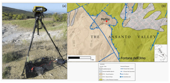
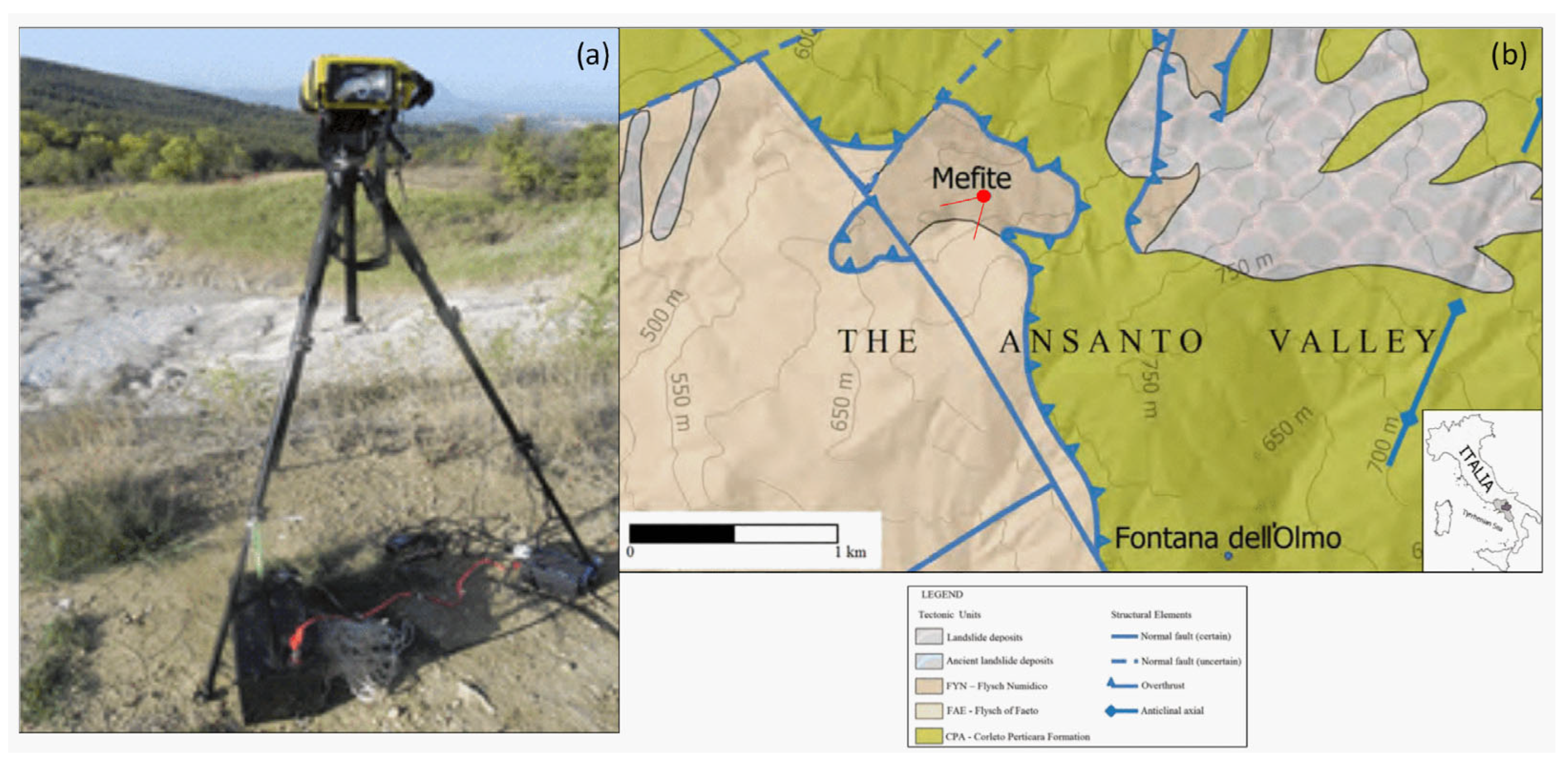
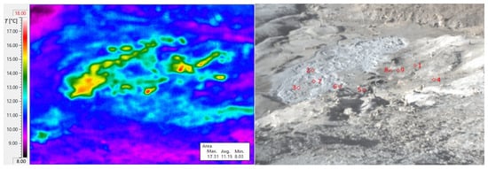
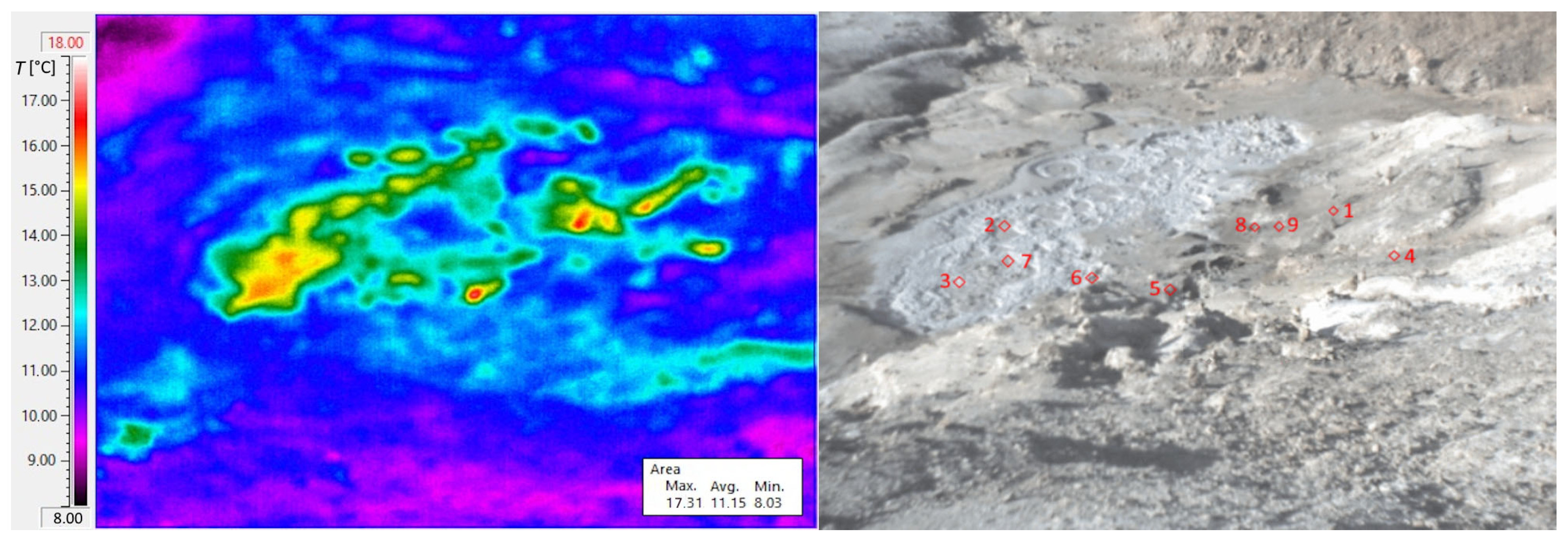
To avoid solar heating, the experiment was conducted at night, around 02:00 LT, once surface effects resulting from sunlight-induced heating had dissipated, and it continued until one hour before dawn (i.e., up to approximately 05:00 LT). The camera operated autonomously for over three hours in an area without electrical power distribution. The internal lithium battery is unsuitable for extended acquisitions, so a lead-acid 12 V, 100 Ah battery-powered supply was integrated into the system. Additionally, to secure the camera and tripod against wind gusts, tie rods were anchored to the ground. Figure 1a is a photo of the monitoring setup, while Figure 1b reports a map indicating the camera’s position relative to the Mefite Lake. Spot positions of sampled temperature time series were selected on site, primarily at the centres of the most prominent gas vents. These positions were considered constants despite slight movements due to erosive processes that could occur over weeks. As previously mentioned, each spot temperature was sampled every minute to detect any rapid variations in gas emissions at this site. The positions of the spots in the Mefite area are shown and numbered in Figure 2. Spots 2, 3, and 7 are located in the puddle, while spots 1, 4–6, 8, and 9 are positioned north of the puddle on dry soil emission vents. Even for short distances, such as those between the camera and the Mefite Lake in this case, TIR imagery can be challenging depending on weather conditions. Thus, a fair-weather day was chosen. Thermal imaging cameras deliver accurate temperature data only after correcting for material emissivity, viewing angle, and atmospheric absorption length, even when measurements are taken from oblique angles.

Figure 1. (a) On-site setup of the VisIR camera; (b) geological map of the Mefite area, extracted from sheet n. 450 “Sant’Angelo dei Lombardi” of the Geological Map of Italy (modified by [28,29]). The camera position and the indicated field of view are shown in red.

Figure 2. Thermal and visible photos taken by VisIR 640; the monitored spots of the thermal image on the (left) are indicated by red squares and numbered in the visible image on the (right).

Even though the emissivity was fixed based on ground composition, the measured IR temperatures are not considered real surface temperatures. The Mefite surface is characterised by soil without vegetation, predominantly clayey-calcareous terrain [30], and a pool occupied by water. Therefore, the first correction of the spot’s temperature time series regards the real materials of spots, with assumed emissivities of 0.39 and 0.67 [26] for spots in clayey-calcareous (1, 4–6, 8, and 9) and water (2, 3, and 7), respectively. We need to take into account the camera’s field-of-view orientation to affect the accuracy of the temperature measurements. Indeed, the source emissivity attenuates when the direction is not perpendicular to the target surface [31], necessitating appropriate corrections. Angular variation arises from the intrinsic properties of materials, which may depend on wavelength, as well as factors such as granularity, surface roughness, and medium porosity. For example, sandy materials exhibit a slight decrease in emissivity with increasing angles. The angular response of natural materials, such as some soils, was investigated under laboratory conditions [31]. Relative emissivity changes are observed between 0.95 and 0.89 at angles between 60° and 80° with the nadir. Moreover, the relative emissivity signature shows an almost flat spectral behaviour, mainly due to soil granularity. At the same time, such granularity influences the angular dependence of emissivity. Instead, the angular response of the water surface produces smaller emissivity changes [32], which are further reduced by the boiling movements of the water surface in the pool. An uncertainty of <1% was considered because studies in [31,32] reported uncertainties of <0.2% and <0.5%, respectively.

Since the VisIR camera views different spots at slightly different angles, different emissivities are expected due to the materials and angles with respect to the nadir. The relative emissivities ε_soil(mud) due to both material (soil or mud) and view angle were summarised in Table 1, column 5: columns 1, 2, 3, and 4 report the spot number, the distance d from the camera, elevation h, and the angle of view to the nadir, respectively. Moreover, the effect of water vapour, described by its absorption coefficient, is considered. Detailed measurements of the absorptivity of mixtures of water vapour in the air were reported for different partial pressures. An absorption coefficient of around 10⁻⁶ cm⁻¹ was retrieved for a water vapour partial pressure of 10 Torr [33], corresponding to an absolute humidity of around 10 g m⁻³ and a relative humidity of around 81.2% for T = 13.5 °C [34]. Transmittance τ_atm = e^−0.1d, with d in km, is reported in column 6 of Table 1. Finally, the spot temperatures can be corrected [35], also considering the humid atmosphere emissivity ε_atm [36], as reported in column 7 of Table 1.

Table 1. The summary of spot distances, altitudes, angles, and corrections; note that spots 2, 3, and 7 have major emissivities due to the presence of water.

Spot	d [m]	h [m]	Angle [°]	ε	τatm	εatm
1	67.36	665	71.83	0.342	0.993	0.727
2	68.35	662	69.44	0.615	0.993	0.727
3	62.77	662	67.52	0.611	0.994	0.727
4	55.36	667	69.93	0.340	0.994	0.727
5	56.08	665	68.01	0.338	0.994	0.727
6	63.32	663	68.70	0.339	0.994	0.727
7	62.77	662	67.52	0.611	0.994	0.727
8	59.81	665	69.44	0.340	0.994	0.727
9	59.81	665	69.44	0.340	0.994	0.727

Furthermore, due to extrinsic field conditions, automatic camera parameter calibration and correction were insufficient to achieve accurate temperature readings. Therefore, an optimal night with stable environmental parameters was chosen for the acquisition survey on 27 October 2022. We applied atmospheric corrections for attenuation based on both viewing distance and relative humidity, retrieved from an adjacent meteorological station in Gesualdo village (41°00′19″ N; 13°04′13″ E), 654 m asl, located about 6.8 km north of Mefite. Data recorded at Gesualdo showed a near-constant temperature of 13.5 °C, with a small variation of around 1 °C; a humidity of 88%; a high pressure of 102.74 kPa; a constant wind speed of 1.1 km h⁻¹; no rain; and fair weather with a sight range of 22 km. The applied equation for the corrections of the measured temperature T_meas to obtain the target (soil or mud) temperature T_targ, given the atmospheric T_atm and background T_back temperatures and related emissivities, is the standard one-layer radiative-transfer correction used for TI temperature retrieval under blackbody behaviour and following [35,36]:

T⁴_targ = [ε_soil(mud)T⁴_meas + (1 − τ_atm − ε_soil(mud) + τ_atmε_atm)T⁴_back +
− (1 − τ_atm)ε_atmT⁴_atm]/τ_atmε_atm

(1)

3. Results

More accurate surface temperature time series were obtained for all points after applying corrections to the thermal imaging camera measurements using relation (1). Instead of assuming a constant emissivity, a reliable analysis has been achieved by using more realistic temperature values that take into account material-dependent emissivity, which varies based on surface type, finish, and wavelength range.

3.1. Real Surface Temperatures

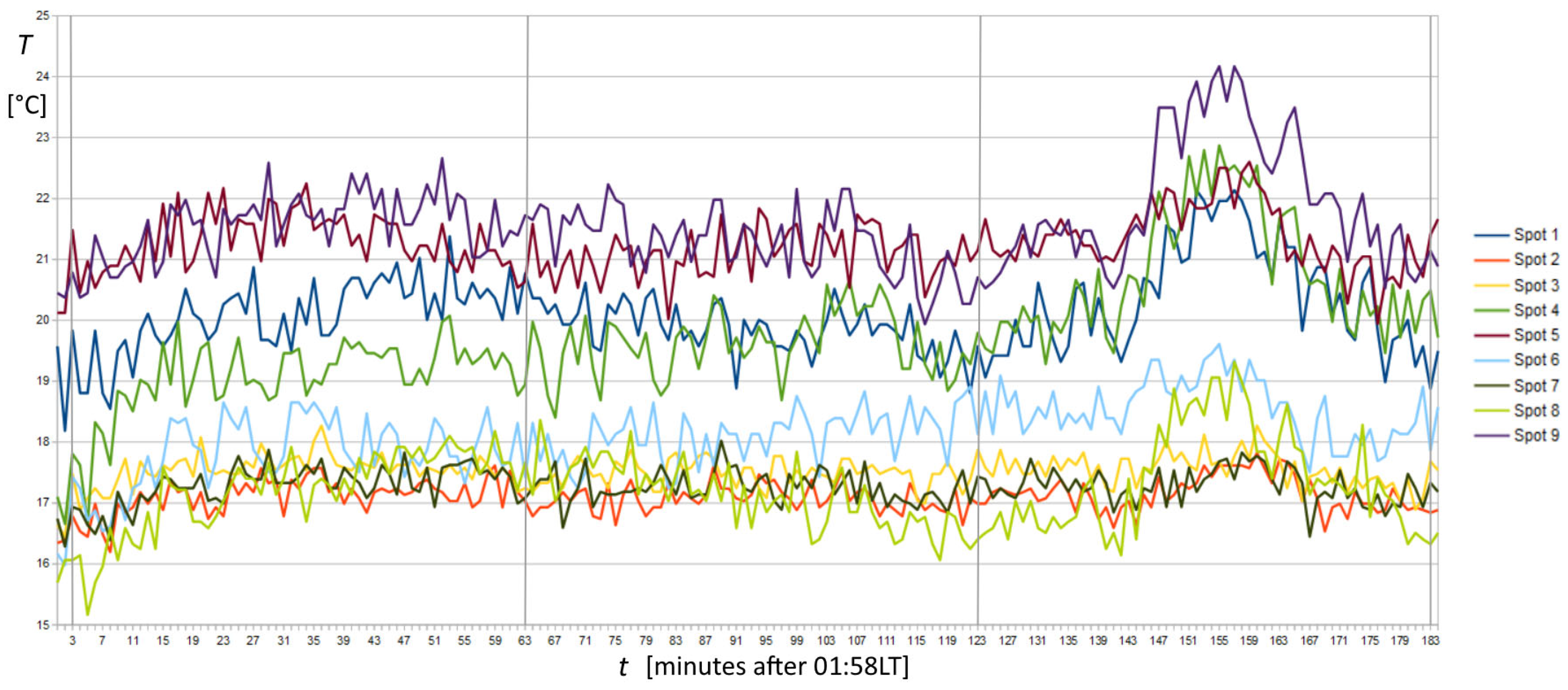
The corrected temperature time series of spots 1 to 9 is shown with different colours in Figure 3. The temperature range of the corrected time series was between 15 and 25 °C, which corresponded to the temperature range of TIR images, between 8 and 18 °C (Figure 2 left). Despite that, temperature differences around 0.2 °C were resolvable in TIR images using an appropriate colour palette. Thus, several active spots appeared outside the puddle with different temperatures in the background. This pattern warranted further investigation, as the area around the puddle was prohibited from direct access due to the high CO₂ concentration, and the detailed pattern of soil degassing was previously unknown. Regarding degassing point positions, they are crucial in evaluating the total CO₂ emission of the Mefite area. In fact, several degassing spots were also observed far from the puddle, at the bottom left and middle right of the thermal image in Figure 2, both about 20–30 m from the puddle. The shape of the spots varied, some appearing rounded and others very elongated. In addition to the 9 spots’ time series investigated, the survey revealed 11 other hotspots where CO₂ emissions are accentuated and are therefore useful for future investigations. On dry soil, spots 1, 4, 5, 6, 8, and 9 appear roughly arranged along a SW-NE direction similar to the longer axis of the puddle and the spots inside it. While some linear-shaped emissions are observed near spots 1 and 4, they are directed perpendicular to this direction.

Figure 3. Plots of the temperature time series corrected by total relative emissivity and humid atmospheric transmittance and emissivity. Vertical grey lines indicate 02:00, 03:00, 04:00, and 05:00 LT. Numbers 1 to 9 correspond to the spot positions in Figure 2, right. A significant temperature peak is observed before the end of the record in spots 1, 4, 8, and 9, far from the puddle, whereas the peak completely disappears in the puddle at spots 2, 3, and 7.

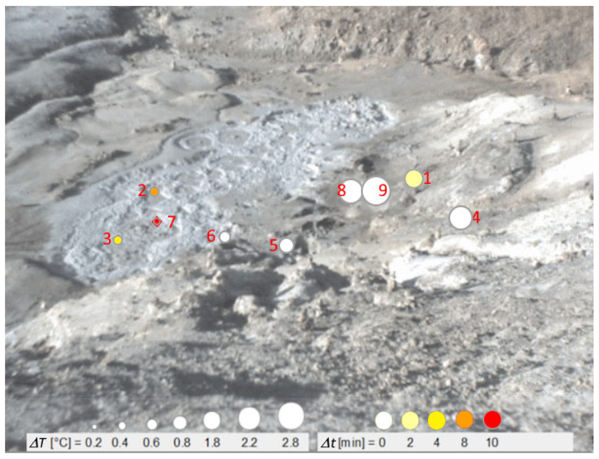
The time series in Figure 3 shows short-term variability and a modest warming trend during the first 20 min of sampling. The most significant temperature increase reached 2.2 °C at spot 4. Other variations are observed in the middle of the recording. Then, a monotonic increase began at around 04:20 and reached its highest value of ΔT = 2.8 °C at 04:35 at spot 9. Shortly after, the temperature decreases, returning to the relative baseline. Focusing on the record at spot 9, as shown in Figure 4, we present a qualitative comparison between that, chosen as the reference, and ΔT measured at spots 1–8. Symbols indicate the respective ΔT and starting time difference (Δt) related to our reference.

Figure 4. Variations from the average temperature regarding the lead times of the observed peak towards the end of the recording in spot 9. Temperature variations are evidenced in the left rectangle and by circle dimensions, whereas lead times are evidenced in the right rectangle and by colours.

3.2. Factor Analysis

Factor analysis ([37] and references therein) was performed using Statistica 10 software (https://statistica.software.informer.com/) on the raw data to identify potential associations between the original variables by searching and extracting new hidden (latent) ones. Three new variables, named “factors”, have been extracted and reported in Table 2 and Table 3. Each factor represents the pattern of correlations among observed variables, evidencing the portion of the total variance in the data system. From Table 3, the first factor accounts for about 55% of the total variance and is represented by spots 1, 8, and 9. The second factor is represented by spots 2, 3, and 7, which together comprise 10.7% of the total variance. Spots 4, 5, and 6 represent the third factor, which accounts for 9.5% of the total variance. The presented model differentiates three relevant groupings of three spot variables, explaining around 75% of the total system variance.

Table 2. Factor analysis conducted on raw data: Loadings (results). Last two rows: Variance for a given factor—the sum of the squares of the loadings across variables for factor—and Proportion of Total Variance, i.e., variance divided by the number of variables.

Spot	Factor 1	Factor 2	Factor 3
1	0.830	0.229	0.290
2	0.411	0.680	0.211
3	0.124	0.743	0.311
4	0.560	0.135	0.682
5	0.179	0.343	0.688
6	0.213	0.183	0.846
7	0.223	0.771	0.112
8	0.866	0.300	0.133
9	0.843	0.230	0.305
Variance	2.776	1.975	2.004
Proportion	0.308	0.219	0.223

Table 3. Factor analysis was conducted on the raw data, which included eigenvalues and factor variances. The eigenvalue represents the total variance of the system expressed in each factor.

Principal Component	Eigenvalue	% Total Variance	Cumulative Eigenvalues	% Cumulative
1	4.943	54.921	4.943	54.921
2	0.959	10.657	5.902	65.578
3	0.854	9.488	6.756	75.066

3.3. FFT and Cluster Analyses

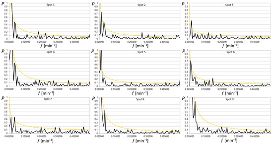
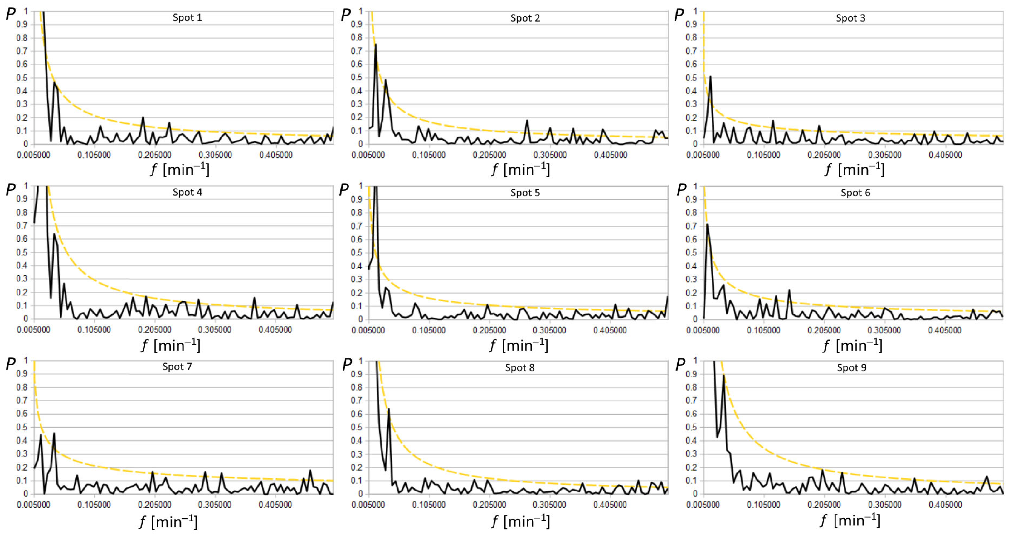
The characteristic oscillations of the system were investigated using FFT applied to the time series of all nine chosen spots, as shown in Figure 5. The resulting periodograms generally follow the fitting function f^−α, where f is the frequency (here in min⁻¹), and α is the fitting exponent, as expected for a thermal system [38]. In this kind of spectrum, higher magnitudes of periodogram values occur at low frequencies. Thus, the appearance of high-magnitude peaks above the noise in the spectra can highlight spurious peaks that are not statistically significant and linked to the sampling procedures themselves, especially when a limited amount of data is insufficient to average the periodogram. Hence, it is crucial to develop robust tests to assess the significance of periodogram peaks. Here, the method described for a series of data characterised by red noise was used [39], estimating the statistical weight of any peaks above the noise and avoiding Monte Carlo simulation.

Figure 5. Periodograms P(f) of the 9 spot signals in black were fitted by power spectra f^−α indicated in coloured continuous lines; dotted yellow lines indicate the 95% peak level of significance above thermal fluctuations. Several periods are evident around 2.1′, 2.6′, 5.0′, 8.0′, 26′, and 61′.

The continuum spectrum I(f) was obtained starting from the periodogram P(f). Least squares fitting has been applied to the logarithm of periodogram values: working with the logarithm, the power model P(f) = N f^−α (where N and α are the two fitting parameters) becomes linear, and the periodogram ordinates become less skewed. Moreover, the expectation value of the logarithm of the periodogram deviates by a constant from that of the logarithm of the spectrum:

<log P(f_j)> = <log I(f_j)> + 0.25068.

(2)

Thus, the fitting linear function y = α x + c can be used on the plot of the spectrum, ignoring the datum at the Nyquist frequency (j = n, where j is the j-th frequency and n is the last frequency, i.e., the Nyquist frequency)

log I(f_j) = log N − 0.25068 − α log f_j,

(3)

and the log N = c + 0.25068 estimates the continuum periodogram for a comparison with the periodogram data. Supposing that I(f_j) is the exact form of the spectrum, the estimates of c and α can be used to formulate the null hypothesis. In other words, if the null hypothesis is true, all peaks are linked to red noise (or to limited sampling). Consequently, the data satisfy the power process with no n’-periodic components. Then, the threshold G for the null hypothesis to be true, with a probability p, results in:

G = −2 ln [1 − (1 − p)^1/n’],

(4)

where G/2 is a multiplicative factor to obtain the threshold for P, and p is called “false alarm probability”. The confidence limit for the nine spots has been fixed at 5%, calculated to evaluate n’-periodic components emerging in each spot series. It is represented in Figure 5 by the dashed-dotted yellow lines. The values of G/2, n’, period and the corresponding test result are reported in Table 4. Common periods occur at 2.1–2.3, 2.6–2.8, 5.0, 26, and 61 min, with the middle peak being the most pronounced among them, while uncommon periods occur at 3.2–3.7, 4.3–4.4, 5.4–5.5, 6.8, 8.0, 8.4 and 31 min.

Table 4. The number of the spot is reported in column 1, the best fit in columns 2 and 3, the tested n’ peaks are reported in column 4, the corresponding periods in column 5, and the test results at a 95% confidence level (t: true, f: false) in column 6; thresholds G/2 are reported in column 7.

Spot	N	a	n’	Periods [min]	Null Hypothesis	G/2
1	0.008046	0.78380	5	92, 61, 26, 5.4, 4.4	f, t, f, f, f	4.58476
2	0.006365	0.74377	7	61, 31, 3.7, 3.3, 2.9, 2.5, 2.1	f, f, f, f, f, f, f	4.91977
3	0.010167	0.46704	5	61, 8.4, 5.1, 2.6, 2.1	f, f, f, f, f	4.58476
4	0.007380	0.93825	6	61, 46, 5.2, 3.6, 2.7, 2.3	f, f, f, f, f, f	4.76623
5	0.009557	0.59826	4	61, 5.0, 2.4, 2.3	f, f, f, f	4.36289
6	0.008733	0.62205	5	92, 61, 8.0, 6.8, 2.2	f, f, f, f, f	4.58476
7	0.015454	0.46930	6	61, 26, 5.0, 3.5, 3.2, 2.1	t, f, f, f, f, f	4.76623
8	0.005346	0.95000	7	92, 61, 26, 5.0, 2.8, 2.2, 2.1	f, f, f, t, f, f, f	4.91977
9	0.008203	0.95000	7	61, 26, 5.0, 4.3, 2.8, 2.6, 2.2	f, f, f, f, f, t, f	4.91977

Spots 1, 8, and 9 are close to, but outside, the puddle. They exhibit the highest amplitude in the first frequency revealed by the spectral analysis, as noted in other works [24], with a cycle of around 92 min, which matches the length of our dataset. Subsequently, they show a well-defined peak at 26 min. Spots 2, 3, and 7 are located within the puddle, characterised by a low amplitude of the first frequency, approximately one-third of the amplitude value of the first spot. Notably, the peak observed here also corresponds to a cycle of roughly 26 min, with spot 7 exhibiting the highest peak. Other medium- and high-frequency periods at 5.0, 4.3, 3.4, and 2.1 min were significantly observed in spots 2, 3, and 7 inside the puddle. They were probably generated by mud bubbles, which move horizontally due to the rising CO₂, whose flow moves from the vertical into the mud pool. However, they have barely detectable amplitudes, just above the level of red noise, suggesting they may have only dubious importance in cycle identification. The last factor describes spots 4, 5, and 6 on land, which have no particularly high frequencies above red noise, except for spot 4, which shows distinct amplitudes corresponding to 3.6, 2.7, and 2.3 min. Upon re-evaluating the factor analysis, it is observable that spot 4 acts as a “bridge” between this group and the first one. This relationship is also evident in the subsequent wavelet analysis.

3.4. Wavelets

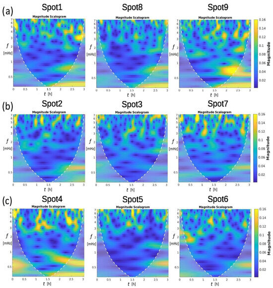
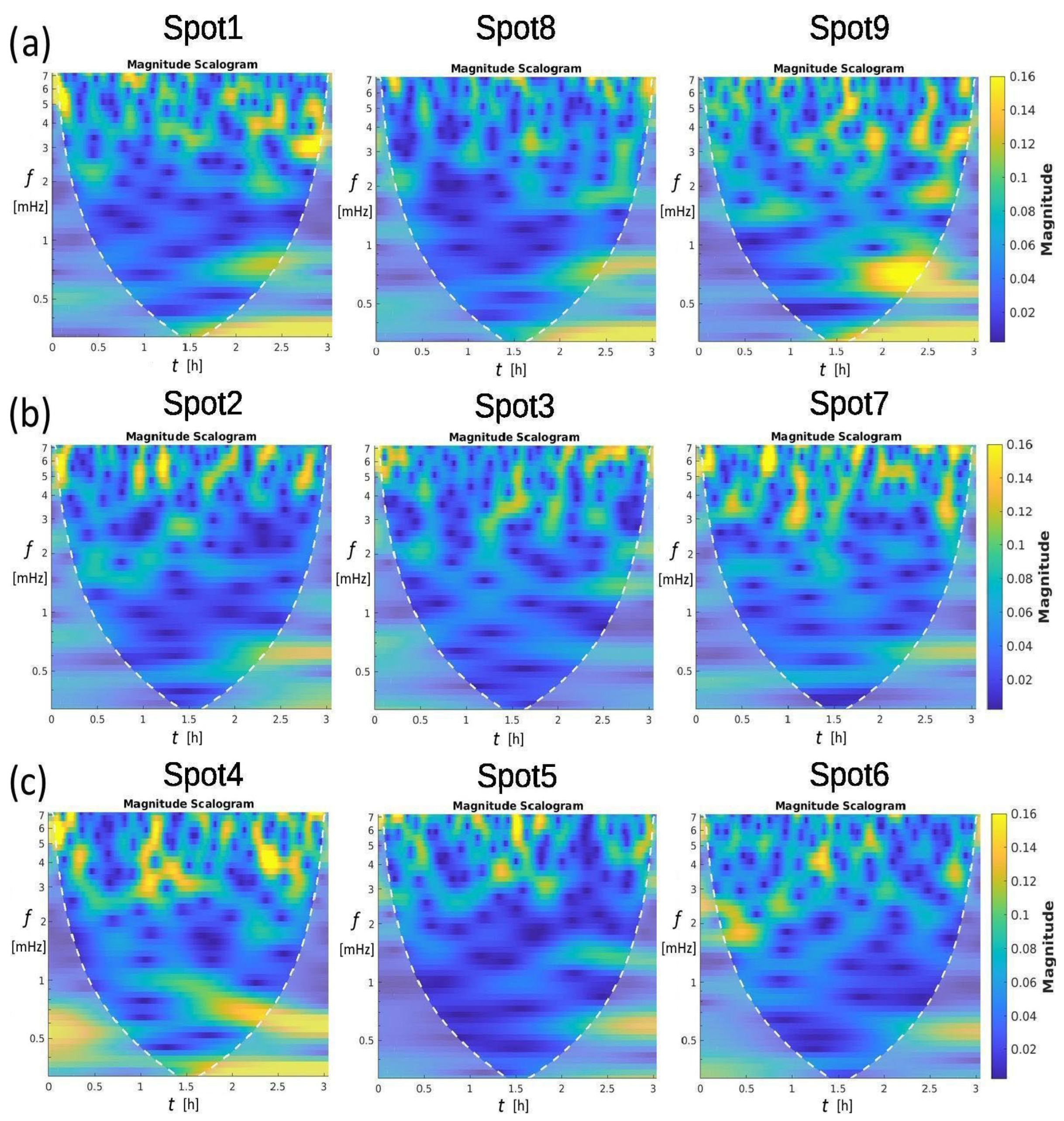
CWT analysis aims to highlight when the already identified peaks occur in the time series and, simultaneously, determine lagging among different spots. The analytic Morse wavelet was applied to the time series shown in Figure 3, with a symmetry parameter, gamma, set to 3 and a time-bandwidth product of 60. Figure 6 shows the results. High-magnitude regions are in yellow, while the blue colour characterises the low-magnitude content within the Cone of Influence, delimited by the white dotted line. Spots 1–9 reveal short-timescale, intermittent degassing dominated by periods of ~2–3 min (5–7 mHz). Spots 4 and 9 display the strongest, most regular bursts consistent with slug-flow or reservoir pressure-release cycles, while spots 2, 3, 5, and 8 show weak, diffuse emission consistent with low-rate bubbling or diffusive degassing. Spots (1, 6, 7) exhibit mixed behaviour. Cross-correlations of burst timing, high-speed visual data, and pressure measurements, along with calibrated flow measurements, could be used to discriminate between slug flow, bubble coalescence, and transient blockage–release mechanisms. Specifically, the spots of the first factor (Figure 6, top) and, more significantly, spots 9 and 4 can be considered representative of the 26 min peak. The 26 min period occurs approximately 120 min after the recording begins and corresponds to the highest ΔT peak measured. Spots belonging to the second factor (Figure 6 middle) appear slightly quieter overall, exhibiting nearly non-existent 26 min periods in the puddle and many low periods. An intermediate scenario of temperature variations is shown at the bottom of Figure 6, corresponding to the third factor, with more pronounced mid-period resonances. Moving along the first column, the 5–6 mHz oscillation is measured at the starting time of spots 1, 2, and 4. The oscillation’s activity tends to be scattered or intermittent over a period of time spanning a few minutes. This behaviour is consistent with vent processes such as bubble bursting, slug/bubble flow, episodic degassing events, or pressure-release pulses rather than steady laminar flow. The spatial heterogeneity (some spots much stronger than others) suggests vent-to-vent differences in geometry, gas supply rate, or local plumbing.

Figure 6. CWT magnitude scalograms were performed with the MATLAB R2022a software (at https://ch.mathworks.com/help/wavelet/ (accessed on 3 March 2026) for nine spatial locations (spots 1–9). Each scalogram illustrates the distribution of signal magnitude across time (0–3 h) and frequency (0–8 mHz). High-magnitude regions (yellow) are predominantly concentrated in the 5–7 mHz band and appear intermittently over the time span, indicating non-stationary and burst-like activity. Spots 4 and 9 exhibit the strongest overall magnitudes, whereas spots 2, 3, 5, and 8 show comparatively weak responses. The white dashed boundary denotes the cone of influence, inside which the wavelet coefficients are least affected by edge effects. The spots in (a) are outside the pool; those in (b) are the three spots inside the pool; those in (c) are on the right pool edge.

3.5. Cross-Correlations

Cross-correlation analysis [40] was performed using Statistica 10 software (https://statistica.software.informer.com/) with a 1 min step. The described temperature growth at the beginning and the large variation at the end were excluded in all spots. We did this to focus the analysis on the smaller fluctuations visible in the central record data. Therefore, we excluded only the first 25 samples of the ramp and the last 45 samples of the peak, considering 115 remaining samples.

The correlations R between pairs of spots of the same factor are positive at lag 0. However, the correlations between pairs of spots from different factors show variable lags, with Δt ranging from 1 to 20 min. This variability in lag occurs even when correlating different spots of the same factor with a spot of another factor. For example, spots 2 and 7 have a 5 min time lag compared to spot 5, whereas spot 3 has a 1 min time lag compared to spot 5. Longer time lags of 15 to 20 min characterise the correlations between spots 3 and 7 with spot 8, respectively.

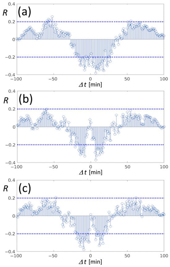
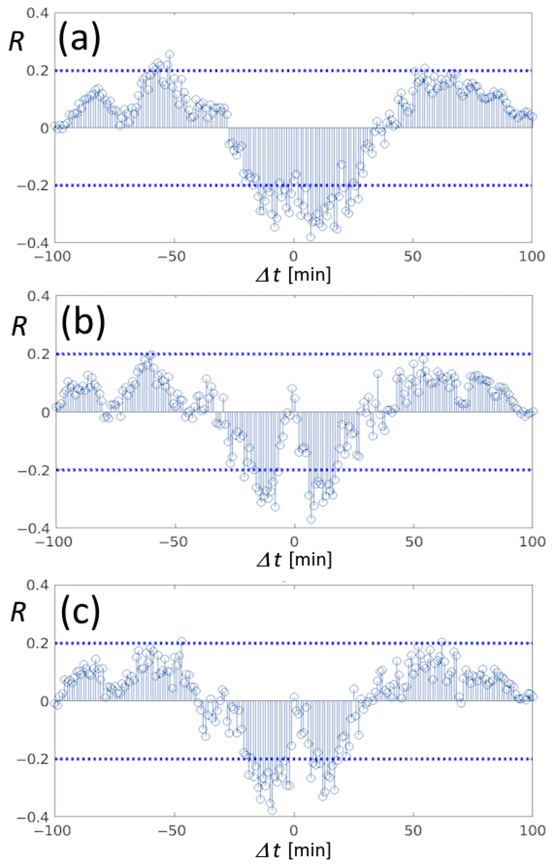
Anti-correlations are also present; they are shown in Figure 7, where horizontal dashed lines indicate the 95% significance level of R. All the spots of the first factor showed anti-correlation with spot 6, with a time lag of 10 min. From Figure 7, spots of the first factor are also anti-correlated with spot 4. Here, only anti-correlations are significant, and their symmetry underscores that these spots are observed to the same pulsation of approximately 5 min. Moreover, the 5 min pulsation of spot 4 is 180° out of phase with spots 9 and 1, as shown in Figure 7b,c, respectively.

Figure 7. Pearson’s correlations between the couples of spots 4-8 (a), 4-9 (b), and 4-1 (c), reporting symmetric anti-correlations of about Δt = ±5 min around the time lag 0 min, describing a 180° phase factor of the 5 min pulsation between spots of the first factor analysed in Figure 6a and the extreme spot 4. Horizontal dashed lines indicate the 95% significance level.

4. Discussion

The Mefite discharging structure is apparently fed by a deep thousand-metre antiform reservoir containing monophasic supercritical CO₂ (scCO₂), as discovered in the 1960s during the national oil-drilling programme [41]. The top of the reservoir has been localised at a depth of around 1128 m. Up to a depth of 1600 m, the main encountered phase is CO₂. Then, from 1600 m to a depth of 1800 m, NaCl-rich water is encountered, with a density of 1.16 g/L and a temperature close to 77 °C; therefore, the related average geothermal gradient is 30 °C km⁻¹.

Following the striking Irpinia earthquake in November 1980, Mw 6.9 [42], and the related seismic aftershock sequence, the regional setting of the epicentre has been extensively studied. The Mefite site has been investigated because it lies on the northern edge of the NW–SE fault activated during the Irpinia earthquake sequence, with particular attention to how its discharge system works and is structured. A four-day seismic array survey showed tremors of variable duration ranging from 20 s to 30–40 min [24]. Moreover, fluctuations in discharge flux were already recorded near spot 9, with values ranging from 418.5 to 440.8 m³ h⁻¹, a variation of less than 6%, in what was defined as a high-pressure vent [43].

Spots 1, 4, 8, and 9 show temporary temperature deviations of nearly 3 °C, with a period of 26 min. If we assume adiabatic compression in a system with approximately constant geometry, a slight gas pressure increase of about 4.3 kPa is sufficient to increase the temperature by 3 °C, according to the adiabatic relation:

T_f = T_i (P_f/P_i)^(γ−1)/γ

(5)

where T_f = 297.34 °K (final temperature); T_i = 294.54 °K (initial temperature); P_f is unknown (final pressure); P_i = 102.74 kPa (initial pressure); and γ = 1.3 (heat capacity ratio). The resulting final pressure is 107.04 kPa, which corresponds to a rise of 4.2%. A possible reason for the increases in flux pressure and temperature could be a temporary increase in deep scCO₂ production and/or an increased release from the anticline structure hosting the free scCO₂ phase. Equation (5) assumes adiabatic compression to link temperature change to pressure change. Moreover, another limitation is that the temperature measured is the surface soil/water temperature, not the gas itself. Assuming ΔT_surface ≈ ΔT_gas is another strong approximation. We admit that both approximations are not perfect, but they can provide a first-order estimate of the final pressure rather than a precise measurement.

In summary, all these fluctuations constitute the common activity of the Mefite emission. The period, whose duration we determined to be around 26 min, is probably linked to a cyclical augmented discharge originating directly from the antiform structure. If we accept as valid the assumption that CO₂ is at hydrostatic pressure, as reconstructed from hydrocarbon exploration well measurements of M. Forcuso 1 and M. Forcuso 2 [44], the discharge starts from CO₂ in its supercritical aggregation phase. At around 700 metres depth, moving upward, it should transform into gas. This transition changes most of its thermodynamic properties, among others, density, internal energy, enthalpy, entropy, adiabatic index, and Joule–Thomson coefficient, as is arguable from the carbon dioxide equation of state [45] and physical characteristics, as is briefly summarised in [46]. Variations measured at shorter periods, as detected in [24], are supposedly linked to the shallow geometry of differentiated escaping routes. Those authors ascribe them to “bubbling episodes”. In this hypothesis, the transition happens mandatorily above 700 metres, i.e., well above the antiform structure. In other words, these short cycles originated not far from the surface, implying the Mefite Lake’s shallow geometry just below the emerging point. The complex behaviour of the spot system, where correlations evidenced pairs of spots alternately exchanging pressure, may be interpretable through channel geometry as a system of communicating vessels excited by the passage of fluid. In any case, the main phenomena detected throughout all spots, and taking into account the conclusions of other authors, seem to have a unique origin.

5. Conclusions

Based on a high-resolution infrared survey, more than 20 natural emissions were identified around the Mefite d’Ansanto pool, the largest natural emitter of CO₂-rich gases with mantle-derived fluids ever measured on Earth. We emphasise that our method provides a non-contact, proximal sensing alternative to direct flux sampling, which is dangerous in high-CO₂ areas such as Mefite. Thus, this methodology can provide a valuable data inventory for future analysis of the chemical and physical activity of the vents in the Mefite Lake and other low-temperature gas emissions. Specifically, the entire Mefite area is degassing, with major emissions from circular and linear vents that mainly align along two near-parallel SW-NE pathways. Moreover, the dominance of the SW-NE trend aligns with the orientation of the previously identified fault [47], while the other elongated vents seem to delineate the surrounding structures. The monitoring revealed extended and concentrated emissions, even with low temperature differences between the ground thermalised gas and the atmosphere. It can be useful to estimate the total CO₂ flux escaping into the atmosphere during future prolonged monitoring.

Moreover, temperature time series of hot spots, retrieved from high-frequency TIR image sampling, appeared not constant, and FFT analysis evidenced periods—from a few minutes to one hour—significantly above red noise. The long period of about 26 min that characterised all the spots confirmed a recurrence observed by seismic studies. Short periods of 2–3 min were observed in the puddle, likely related to horizontal bubble movements. Statistical association divided the spots into three groups whose behaviours explained 75% of the variability, and wavelet analysis confirmed this association. The presence of water seems to relate such variability to the channel configuration beneath the spots. Moreover, statistical correlations confirmed shifts between pairs of spots and some complexity in the exchange of gas flux among other spots.

All the limitations in retrieving absolute temperature were considered, even if they did not compromise the investigation of relative spatio-temporal variations in Mefite Lake. Instead, precision was significant when a thermodynamic discussion described temperature variations as variations in gas pressure across the spots. This allowed us to determine that a 4.2% increase in pressure was responsible for the 2.8 °C increase in temperature at spot 9, the one with major emission. This result underscores how TIR monitoring can provide an indirect and sensitive measure of gas pressure variations, even at cold vents. Finally, this represents the first example of high-frequency TIR sampling applied to the Mefite d’Ansanto or to any low-temperature gas emission, including cold vents.

References

- Chiodini, G.; Granieri, D.; Avino, R.; Caliro, S.; Costa, A.; Minopoli, C.; Vilardo, G. Non-volcanic CO2 Earth degassing: Case of Mefite d’Ansanto (southern Apennines), Italy. Geophys. Res. Lett. 2010, 37, L11303. [Google Scholar] [CrossRef] [Scilit]
- Improta, L.; De Gori, P.; Chiarabba, C. New insights into crustal structure, Cenozoic magmatism, CO2 degassing, and seismogenesis in the southern Apennines and Irpinia region from local earthquake tomography. J. Geophys. Res. Solid Earth 2014, 119, 8283–8311. [Google Scholar] [CrossRef] [Scilit]
- Nicotra, E.; Passaro, S.; Ventura, G. The formation and growth mechanisms of young back-arc spreading ridges from high-resolution bathymetry: The Marsili Seamount (Tyrrhenian Sea, Italy). Geosci. Front. 2024, 15, 101723. [Google Scholar] [CrossRef] [Scilit]
- Farolfi, G.; Piombino, A.; Catani, F. Fusion of GNSS and Satellite Radar Interferometry: Determination of 3D Fine-Scale Map of Present-Day Surface Displacements in Italy as Expressions of Geodynamic Processes. Remote Sens. 2019, 11, 394. [Google Scholar] [CrossRef] [Scilit]
- Palano, M.; Cannavò, F.; Ferranti, L.; Mattia, M.; Mazzella, M. Strain and stress fields in the Southern Apennines (Italy) constrained by geodetic, seismological and borehole data. Geophys. J. Int. 2011, 187, 1270–1282. [Google Scholar] [CrossRef] [Scilit]
- Piombino, A.; Bernardini, F.; Farolfi, G. Assessing Current Seismic Hazards in Irpinia Forty Years after the 1980 Earthquake: Merging Historical Seismicity and Satellite Data about Recent Ground Movements. Geosciences 2021, 11, 168. [Google Scholar] [CrossRef] [Scilit]
- Giustini, F.; Brilli, M. Mefite d’Ansanto, southern Apennines (Italy): The natural CO2 seep which emits the largest quantity of non-volcanic CO2 on Earth. Int. J. Earth Sci. 2020, 109, 1705–1706. [Google Scholar] [CrossRef] [Scilit]
- Italiano, F.; Martelli, M.; Martinelli, G.; Nuccio, P.M. High 3He gas emissions from the Irpinian Apennine: Mantle relations and genetic hypothesis. Nuovo Cim. C 1999, 22C, 373–378. [Google Scholar]
- Italiano, F.; Martelli, M.; Martinelli, G.; Nuccio, P.M. Geochemical evidence of melt intrusions along lithospheric faults of the Southern Apennines, Italy: Geodynamic and seismogenic implications. J. Geophys. Res. 2000, 105, 13569–13578. [Google Scholar] [CrossRef] [Scilit]
- Caracausi, A.; Paternoster, M.; Nuccio, P.M. Mantle CO2 degassing at Mt. Vulture volcano (Italy): Relationship between CO2 outgassing of volcanoes and the time of their last eruption. Earth Planet. Sci. Lett. 2015, 411, 268–280. [Google Scholar] [CrossRef] [Scilit]
- Caracausi, A.; Sulli, A. Outgassing of mantle volatiles in compressional tectonic regime away from volcanism: The role of continental delamination. Geochem. Geophys. Geosyst. 2019, 20, 2007–2020. [Google Scholar] [CrossRef] [Scilit]
- Sbrana, A.; Marianelli, P.; Belgiorno, M.; Sbrana, M.; Ciani, V. Natural CO2 degassing in the Mount Amiata volcanic–geothermal area. J. Volcanol. Geotherm. Res. 2020, 397, 106852. [Google Scholar] [CrossRef] [Scilit]
- Chiodini, G.; Cardellini, C.; Amato, A.; Boschi, E.; Caliro, S.; Frondini, F.; Ventura, G. Carbon dioxide Earth degassing and seismogenesis in central and southern Italy. Geophys. Res. Lett. 2004, 31, L07615. [Google Scholar] [CrossRef] [Scilit]
- Frezzotti, M.; Peccerillo, L.; Panza, A.; Panza, G.F. Carbonate metasomatism and CO2 lithosphere-asthenosphere degassing beneath the western Mediterranean: An integrated model arising from petrological and geophysical data. Chem. Geol. 2009, 262, 108–120. [Google Scholar] [CrossRef] [Scilit]
- Cianchini, G.; Fidani, C.; Piscini, A.; Sabbagh, D.; Soldani, M. The audio and electrical monitoring of the Mefite area in the ELF band. In Proceedings of the Gruppo Nazionale di Geofisica della Terra Solida (GNGTS), Ferrara, Italy, 13–16 February 2024. [Google Scholar]
- La Rocca, M.; Galluzzo, D.; Nardone, L.; Malagnini, L. Hydrothermal Seismic Tremor in a Wide Frequency Band: The Non-Volcanic CO2 Degassing Site of Mefite d’Ansanto, Italy. Bull. Seismol. Soc. Am. 2023, 113, 1102–1114. [Google Scholar] [CrossRef] [Scilit]
- Wright, R.; Flynn, L.P.; Garbeil, H.; Harris, A.J.; Pilger, E. Near-real-time thermal monitoring of global volcanism. J. Volcanol. Geotherm. Res. 2004, 135, 29–49. [Google Scholar] [CrossRef] [Scilit]
- Silvestri, M.; Romaniello, V.; Hook, S.; Musacchio, M.; Teggi, S.; Buongiorno, M.F. First Comparisons of Surface Temperature Estimations between ECOSTRESS, ASTER and Landsat 8 over Italian Volcanic and Geothermal Areas. Remote Sens. 2020, 12, 184. [Google Scholar] [CrossRef] [Scilit]
- Silvestri, M.; Diaz, J.A.; Rabuffi, F.; Romaniello, V.; Musacchio, M.; Corrales, E.; Fox, J.; Marotta, E.; Belviso, P.; Avino, R.; et al. MultiGAS Detection from Airborne Platforms on Italian Volcanic and Geothermal Areas. Remote Sens. 2023, 15, 2390. [Google Scholar] [CrossRef] [Scilit]
- Stevenson, J.A.; Varley, N. Fumarole monitoring with a handheld infrared camera: Volcán de Colima, Mexico, 2006–2007. J. Volcanol. Geotherm. Res. 2008, 177, 911–924. [Google Scholar] [CrossRef] [Scilit]
- Sekioka, M.; Yuhara, K. Heat flux estimation in geothermal areas based on the heat balance of the ground surface. J. Geophys. Res. 1974, 79, 2053–2058. [Google Scholar] [CrossRef] [Scilit]
- Marotta, E.; Peluso, R.; Avino, R.; Belviso, P.; Caliro, S.; Carandente, A.; Chiodini, G.; Macedonio, G.; Avvisati, G.; Marfè, B. Thermal Energy Release Measurement with Thermal Camera: The Case of La Solfatara Volcano (Italy). Remote Sens. 2019, 11, 167. [Google Scholar] [CrossRef] [Scilit]
- Vilardo, G.; Sansivero, F.; Chiodini, G. Long-term TIR imagery processing for spatiotemporal monitoring of surface thermal features in volcanic environment: A case study in the Campi Flegrei (Southern Italy). J. Geophys. Res. Solid Earth 2015, 120, 812–826. [Google Scholar] [CrossRef] [Scilit]
- Panebianco, S.; Satriano, C.; Vivone, G.; Picozzi, M.; Strollo, A.; Stabile, T.A. Automated detection and machine learning-based classification of seismic tremors associated with a non-volcanic gas emission (Mefited’Ansanto, Southern Italy). Geochem. Geophys. Geosyst. 2024, 25, e2023GC011286. [Google Scholar] [CrossRef] [Scilit]
- Thermoteknix Systems Ltd., Cambridge, UK, March 2010, 159395657-Scientific-Visir-640s-Thermal-Camera.pdf. Available online: https://www.thermoteknix.com/support (accessed on 3 March 2026).
- Calex Electronix Limited, Emissivity Tables 2015. Available online: https://www.calex.co.uk/site/wp-content/uploads/2015/07/emissivity-tables.pdf (accessed on 3 March 2026).
- Spampinato, L.; Oppenheimer, C.; Calvari, S.; Cannata, A.; Montalto, P. Lava lake surface characterization by thermal imaging: Erta ’Ale volcano (Ethiopia). Geochem. Geophys. Geosyst. 2008, 9, Q12008. [Google Scholar] [CrossRef] [Scilit]
- ISPRA–Servizio Geologico d’Italia. Carta Geologica d’Italia Alla Scala 1:50.000. Foglio n. 450 “Sant’Angelo dei Lombardi”; CNR: Roma, Italy; ISPRA: Roma, Italy, 2014. [Google Scholar]
- Sisto, M.; Di Lisio, A.; Russo, F. The Mefite in the Ansanto Valley (Southern Italy): A Geoarchaeosite to Promote the Geotourism and Geoconservation of the Irpinian Cultural Landscape. Geoheritage 2020, 12, 29. [Google Scholar] [CrossRef] [Scilit]
- Di Nocera, S.; Imperato, M.; Matano, F.; Stanzione, D.; Valentino, M.G. Caratteri geologici e idrogeochimici della valle di Ansanto (Irpinia Centrale, Appennino Campano-Lucano). Boll. Della Soc. Geol. Ital. 1999, 118, 395–406. [Google Scholar]
- Labed, J.; Stoll, M. Angular variation of land surface spectral emissivity in the thermal infrared: Laboratory investigations on bare soils. Int. J. Remote Sens. 1991, 12, 2299–2310. [Google Scholar] [CrossRef] [Scilit]
- Cuenca, J.; Sobrino, J.A. Experimental measurements for studying angular and spectral variation of thermal infrared emissivity. Appl. Opt. 2004, 43, 4598–4602. [Google Scholar] [CrossRef] [Scilit]
- Shumate, M.S.; Menzies, R.T.; Margolis, J.S.; Rosengren, L.-G. Water vapor absorption of carbon dioxide laser radiation. Appl. Opt. 1976, 15, 2480–2488. [Google Scholar] [CrossRef] [Scilit]
- Khare, S.; Singh, M.; Kaushik, B.K. Range Performance Modelling of Thermal Imaging System based on Single Parameter Characterised by Ambient Temperature and Relative Humidity. Def. Sci. J. 2018, 68, 480–486. [Google Scholar] [CrossRef] [Scilit]
- Minkina, W.; Dudzik, S. Infrared Thermography: Errors and Uncertainties; John Wiley & Sons, Ltd.: Chichester, UK, 2009. [Google Scholar]
- Centeno, V.M. New formulae for the equivalent night sky emissivity. Sol. Energy 1986, 28, 489–498. [Google Scholar] [CrossRef] [Scilit]
- Mathai, A.M.; Provost, S.B.; Haubold, H.J. Factor Analysis. In Multivariate Statistical Analysis in the Real and Complex Domains; Springer: Cham, Switzerland, 2022; pp. 679–710, Correction in Mathai, A.M. Multivariate Statistical Analysis in the Real and Complex Domains; Springer: Cham, Switzerland, 2023. [Google Scholar] [CrossRef] [Scilit]
- Storch, H.V.; Zwiers, F.W. Statistical Analysis in Climate Research; Cambridge University Press: Cambridge, UK, 2010. [Google Scholar]
- Vaughan, S. A simple test for periodic signals in red noise. Astron. Astrophys. 2005, 431, 391–403. [Google Scholar] [CrossRef] [Scilit]
- Box, G.E.P.; Jenkins, J.M.; Reinsel, G.C. Time Series Analysis: Forecasting and Control, 3rd ed.; Prentice Hall: Englewood Cliffs, NJ, USA, 1994. [Google Scholar]
- ViDEPI Project. Ministry for Economic Development DGRME—Italian Geological Society—ASSOMINERARIA, 2012. Visibility of Petroleum Exploration Data in Italy. Available online: https://www.videpi.com/videpi/pozzi/dettaglio.asp?cod=3920 (accessed on 3 March 2026).
- Improta, L.; Bonagura, M.; Capuano, P.; Iannaccone, G. An integrated geophysical investigation of the upper crust in the epicentral area of the 1980, Ms=6.9, Irpinia earthquake (Southern Italy). Tectonophysics 2003, 361, 139–169. [Google Scholar] [CrossRef] [Scilit]
- Panebianco, S. Fluid Injections in the Subsurface: A Multidisciplinary Approach for Better Understanding Their Implications on Induced Seismicity and the Environment. Ph.D. Thesis, Università degli Studi della Basilicata, Potenza, Italy, 2022. Available online: https://hdl.handle.net/11563/154467 (accessed on 3 March 2026).
- Vitagliano, E.; Improta, L.; Pizzino, L.; D’AGostino, N. Study of well data reveals fluid pressure distribution and origin in the upper crust of the Irpinia region. Tectonophysics 2025, 908, 230761. [Google Scholar] [CrossRef] [Scilit]
- Span, R.; Wagner, W. A New Equation of State for Carbon Dioxide Covering the Fluid Region from the Triple-Point Temperature to 1100 K at Pressures up to 800 MPa. J. Phys. Chem. Ref. Data 1996, 25, 1509–1596. [Google Scholar] [CrossRef] [Scilit]
- Calcara, M. Under Pressure: The Dividing Widom Zone and Possible Consequences on Dry scCO2–Rock Interaction Due to Varying Dipole Moment. Geosciences 2026, 16, 137. [Google Scholar] [CrossRef] [Scilit]
- Pischiutta, M.; Anselmi, M.; Cianfarra, P.; Rovelli, A.; Salvini, F. Directional site effects in a non–volcanic gas emission area (Mefite d’Ansanto, southern Italy): Evidence of a local transfer fault transversal to large NW–SE extensional faults? Phys. Chem. Earth 2013, 63, 116–123. [Google Scholar] [CrossRef] [Scilit]
Disclaimer/Publisher’s Note: The statements, opinions and data contained in all publications are solely those of the individual author(s) and contributor(s) and not of MDPI and/or the editor(s). MDPI and/or the editor(s) disclaim responsibility for any injury to people or property resulting from any ideas, methods, instructions or products referred to in the content. |
© 2026 by the authors. Licensee MDPI, Basel, Switzerland. This article is an open access article distributed under the terms and conditions of the Creative Commons Attribution (CC BY) license.