


Abstract
Assessing the reliability of corroded onshore pipelines represents a spatial and temporal challenge. Pipe operators seek to estimate segment degradation and design an effective maintenance plan with imperfect information, where multiple failure modes can occur. This paper proposes a probabilistic framework for assessing segment reliability, incorporating the spatio-temporal variability of corrosion defects. Based on In-Line Inspection (ILI) measurements, critical segments are identified along the pipeline using a preliminary condition-based segmentation with a changepoint algorithm and two simultaneous failure modes, i.e., small leaks and bursts, with an inverse Gaussian process for the temporal degradation. Reliability is assessed by considering dependent failure limit states using a copula approach with Monte Carlo simulations. The proposed methodology is evaluated on a 60 km pipeline section to characterize spatial variability. The robustness and effectiveness of the changepoint approach in characterizing the spatial variability of corrosion defects as well as in identifying and locating critical segments along the pipeline is well demonstrated. The findings show that evaluating the dependence of pipeline failure events using the copula approach yields to a more realistic estimate of pipeline reliability. In addition, it was found that ignoring spatial variability and failure mode interdependence leads to overly pessimistic estimates, consequently leading to premature maintenance.
1. Introduction
Pipelines transporting hydrocarbons (gas and oil) are considered the most efficient and least expensive over long distances. However, they are subjected to spatial and temporal degradation processes, such as corrosion, which make them challenging to operate. Onshore pipelines are commonly made of steel, and corrosion is one of their main degradation mechanisms, affecting both the inner and outer walls. Corrosion is an electrochemical process that reduces the effective wall thickness of the pipeline material due to environmental exposure or the fluids being transported [1]. Soil corrosivity around the pipeline determines how severe this metal consumption is on the outer side, including of acidity, aeration, pH, texture, among others [2]. Regarding the inner side, fluid properties and operating parameters influence this degradation process, such as pressure, temperature, pH, microorganism activity, or the composition of corrosive components (e.g., CO2 or H2S) [2]. In either case, corrosion is represented in different ways, but the main types are uniform and pitting corrosion. Uniform corrosion is characterized by the loss of material at a similar rate across extensive areas of the pipeline’s inner or outer surfaces. In contrast, pitting corrosion is defined by accelerated material loss in localized regions compared to the surrounding areas. This localized corrosion can form small holes that may expand over time and ultimately cause pipeline failure [3].
Corrosion reduces the pipeline wall’s ability to withstand operational conditions, thereby reducing its effective lifetime. In this regard, In-Line Inspection (ILI) tools, such as Magnetic Flux Leakage (MFL) and Ultrasonic tools (UT), are commonly used to identify, size, and locate corrosion defects along the pipeline either at the inner or outer side of the pipe. In this regard, corrosion defects are described by their depth, length, and width. They are located using the pipeline abscissa and a 12-clock position analogy for orientation. Pipeline operators receive this information from inspection vendors (e.g., Rosen) describing the location and orientation, structural parameters, and the primary descriptors of the detected defects [4]. This information enables pipeline operators to assess and monitor pipeline segment degradation over time based on the remaining wall thickness [1], seeking a safer and more reliable operation. However, these measurements are affected by measurement errors, further complicating maintenance decision-making [3].
Given this complex degradation process, researchers have paid attention to different reliability assessments of corroded pipelines. From a temporal perspective, several models have been proposed to predict the growth of corrosion defects over time. Some approaches use linear models, assuming constant or probabilistic increments between consecutive inspection intervals, as recommended by the National Association of Corrosion Engineering (NACE) [5] or in the work proposed by Pandey [6]. Other alternatives consider non-linear growth rates following a power law function [7], or probabilistic methods that incorporate pipe structural and environment soil variables as random variables [8,9,10,11]. In addition, corrosion growth has also been modeled as a stochastic process because it can capture the temporal variability of corrosion defects. Some examples include the Gamma process [12], Markov Chains [13], and the inverse Gaussian process [14]. Recently, other approaches have also incorporated machine learning to assess the risk of pipeline failure due to leaks [15]. These approaches usually consider the corrosion extent (i.e., depth and length), which can be measured through ILI runs. However, while machine learning algorithms can predict failure probabilities, they function as black-box models that require dense continuous environmental monitoring. In contrast, stochastic processes such as Gamma or inverse Gaussian directly model monotonic, non-negative depth-growth trajectories over time while accommodating sizing errors from routine ILI data.
The reliability assessment is also affected from a spatial point of view. Corroded segments exhibit varying levels of degradation driven by operating conditions, surrounding soil, and pipe properties. Therefore, more specific reliability assessments incorporating these variations are required. In this direction, Amaya-Gómez et al. [2] evaluated a statistical soil characterization using a Multiple Correspondence Analysis (MCA) and K-modes to describe soil properties where more severe defects were found. These authors also proposed a dynamic segmentation of corrosion defects to identify critical segments, requiring interventions [16], and condition-based segmentation using a changepoint algorithm to identify pipe segments with similar degradation [17]. In addition, other alternatives have considered using random fields to evaluate the space-dependent degradation process. Sahraoui and Chateauneuf [18] proposed a probabilistic methodology for assessing the reliability of corroded pipelines subject to space-variant soil aggressiveness. They modeled soil spatial variability as a correlated stochastic field using the Karhunen–Loeve expansion. Xiao et al. [19] also contemplated a random field and examined how its length scale and the correlation of the defect measurements affect the pipeline reliability. Meneses-Gelves et al. [20] introduced a Gaussian random field to characterize the spatial variability of corrosion depth defects obtained by matching consecutive ILI measurements. Consequently, the authors estimated the Mean Time to Failure (MTTF) for each segment, enabling identification of the most critical pipeline segments. Overall, these approaches focused on only one failure mode, principally associated with a burst scenario, and few also include included leakage failure. As noted by CSA Z662 [21] and authors such as Zhou et al. [22], depending on defect depth and length, different failure scenarios such as minor leaks, large leaks or ruptures can occur.
This reliability analysis is also affected by possible correlations among features. In this regard, researchers have increasingly incorporated copula functions into pipeline reliability analysis to model the complex interdependencies among stochastic variables, moving beyond traditional assumptions of mutual independence that can lead to significant errors in failure probability [22,23]. Copula theory provides a flexible framework for modeling asymmetric dependence between parameters, which is common in most situations in corrosion defect scenarios. Different types of copula functions also allow us to better represent dependence between variables [24]. This methodology contemplates critical parameters such as the correlation between pipe diameter and wall thickness, the relationship between initial defect dimensions and their stochastic growth rates over time [19]. Furthermore, copulas characterize dependence between competing failure modes—specifically small leaks and catastrophic bursts—both fundamentally driven by corrosion depth progression [25]. However, while some research acknowledges that multiple defects within similar environmental regions may exhibit spatial correlation [19,26], many current works prioritize a reliability assessment from a distribution perspective, fitting large inspection datasets to stochastic variables without explicitly modeling geographical variability [12,15]. Consequently, a significant research gap remains in developing comprehensive frameworks that simultaneously contemplate spatial variability, stochastic degradation, and joint failure modes using copula functions.
To overcome these limitations, this paper introduces a comprehensive probabilistic framework to evaluate the reliability of pipeline segments by incorporating the spatio-temporal variability of corrosion defects. To capture spatial heterogeneity in corrosion parameters (i.e., depth and length along the pipeline), this work implements a dynamic condition-segmentation framework based on the changepoint approach to identify specific degradation processes in similar affected segments. Then, the segments that are prone to failure will be identified and localized along the pipeline. Furthermore, the temporal evolution of depth defects will be modeled as an inverse Gaussian process. The failure modes will be treated as dependent, and copula theory will be used to characterize the dependence structure.
The proposed framework contemplates the following features:
- A dynamic segmentation contemplating the changepoint algorithm approach based on ILI measurements is implemented. Spatial variability of corrosion defects is evaluated to identify pipeline segments with statistically homogeneous behavior.
- The temporal variability of defects is modeled using an inverse Gaussian process-based stochastic degradation approach. The time-variant reliability of individual segments and the entire pipeline is assessed using Monte Carlo Simulation (MCS).
- Burst and leak failure criteria are considered as dependent events. For this purpose, a copula approach has been incorporated. These failure criteria allow identifying and localizing critical segments along the pipeline for further maintenance.
The remainder of this paper is structured as follows: Section 2 presents a reliability analysis based on the changepoint approach, and introduces the degradation model and the copula theory. Section 3 describes the application of the proposed methodology and discusses the corresponding results. Finally, a conclusion and remarks are given in the last section.
2. Proposed Spatio-Temporal Reliability Assessment of Corroded Pipelines
2.1. Pipeline Segmentation Using the Changepoint Approach
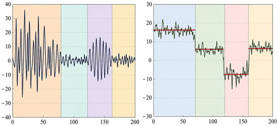
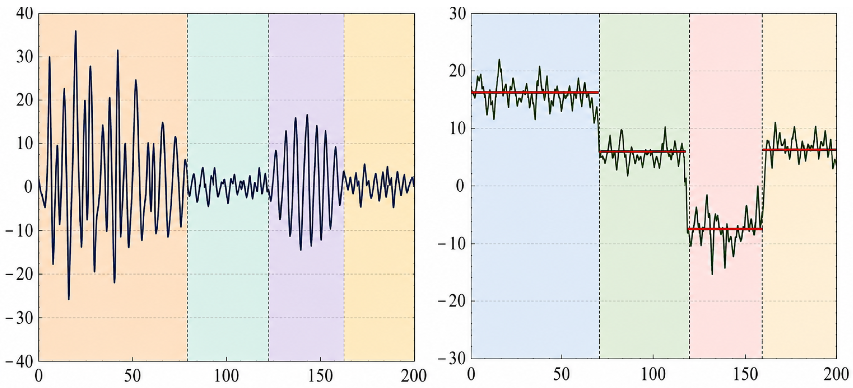
Underground pipelines are complex systems whose reliability evolves under heterogeneous soil conditions along their segments. To address this complexity, various segmentation approaches have been proposed, including soil-based segmentation [18] and fixed-distance segmentation as in [27,28]. However, these methods have some limitations: soil-based approaches require detailed small-scale characterization to adequately capture heterogeneity, while fixed-distance methods cannot adapt to spatial variations in corrosion aggressiveness. To address these limitations, the changepoint approach proposed by Amaya-Gómez et al. [17] was employed. This approach divides the pipeline into segments with similar statistical moments (i.e., mean or variance), see the jumps in Figure 1, which are characterized using corrosion defect measurements obtained from In-Line Inspections.
Figure 1.
Changepoint approach based on the variance (left) and the mean (right) of the corrosion data. Adapted from Amaya-Gómez et al. [17].
This segmentation helps reduce the complexity of reliability assessment and identify critical segments along the pipeline. The changepoints approach uses the Pruned Exact Linear Time method [29] to detect the jumps or change points along the pipeline. For this purpose, the Changepoint for a Range of Penalties (CROPS) algorithm [30] is contemplated, which determines the optimal number of segments based on a penalty value to avoid overfitting. For more details on the changepoint approach, the reader is referred to Ref. [17]. The CROPS algorithm penalizes model complexity by evaluating a range of penalty values to prevent overfitting noisy inspection signals with minor, statistically insignificant changepoints [30]. By identifying the point of maximum curvature on the segmentation cost curve, it selects an optimal partition that cleanly isolates statistically distinct, highly aggressive corrosion clusters without over-segmenting the pipeline [17].
2.2. Failure Modes and Limit States
A pipeline can be modeled as a series system of multiple components (pipe segments), each containing multiple corrosion defects with varying degradation levels. If a segment fails (loss of containment), the whole system fails, requiring an emergency shutdown and disrupting normal fluid transportation. Each segment is assumed to be subject to two failure modes simultaneously: small leaks and bursts.
The limit state function induced by a small leak is denoted as follows [19]:
where is the depth of the corrosion defect at time and represents the thickness of the pipe wall. Note that 80% of the wall thickness is commonly accepted as a leakage limit state; however, some variations exist, such as the one reported by the Canadian Standards Association, using a limit state.
Pipelines are also subjected to a second limit state of a burst [31], in which the operating conditions lead the pipe wall to bulge outward and reach a point of instability. In this case, the limit state function is defined as the difference between the resistance of the burst pressure and the operating pressure , which can be expressed as follows [19]:
Several empirical and semi-empirical models for evaluating the burst pressure have been reported in the literature [31,32]. The evaluation of burst pressure () in corroded pipelines is primarily divided between traditional standard codes based on empirical NG-18 equations with rectangular or parabolic defect idealizations (e.g., ASME B31G, Modified B31G [33], and CSA Z662) and advanced numerical or dimensional analysis models—including 3D non-linear finite element modeling (FEM), Buckingham pi theorem regressions, and strain-hardening formulations—which represent defects with elliptical or complex profiles [32]. While traditional standards tend to produce overly conservative failure predictions for modern ductile materials, models specifically calibrated for moderate-to-high toughness pipelines (grades X52 to X80+), including Netto et al. [34], PCORRC [35,36], Ma et al., and Chen et al. [37], have provided markedly superior accuracy because plastic collapse in high-grade steels is governed by ductile failure rather than notch-sensitive stress states [32]. From these approaches, Netto et al.’s [34] model was derived using Buckingham’s pi theorem alongside 3D non-linear FE simulations and small-scale experiments for elliptical defects in moderate-to-high toughness steels (API 5L X52 to X77). Unlike standard ASME approaches, Netto’s formulation assigns significantly greater importance to relative defect depth (d/w), effectively correcting the tendency of conventional codes to underestimate remaining pipe strength for short defects and overestimate it for long defects. Consequently, comparative reliability and experimental evaluations demonstrate that Netto’s model provides realistic, less conservative predictions, achieving the lowest coefficient of variation (CoV) among evaluated models and delivering highly accurate mean predicted-to-test pressure ratios of 0.91 for moderate-toughness steels and 0.97 for high-toughness steels [32]. For more details on the applicability and conservatism levels of these models, see Ref. [32]. This model was chosen because it is suitable for estimating the burst pressure of high-toughness pipes, such as API X 65, which applies to our case study. This model depends on information regarding the corrosion geometry and pipeline geometry, as well as its mechanical properties; the burst pressure of corroded pipeline segments is given as follows:
where and are the pipe’s outside diameter and wall thickness, respectively. is the pipe’s yield strength, and is associated with the initial corrosion length (last inspection), given that only one ILI run is available. This model is selected because it has been considered as having less conservative predictions than the other models [38].
2.3. Degradation Model
The corrosion growth model through the thickness of the pipeline wall is modeled as a stochastic process, specifically as an inverse Gaussian process. The advantage of the inverse Gaussian process is that it is defined for positive values and can characterize the temporal variability of defect depth growth. It is described as follows:
where represents the initial depth of the corrosion defect in segment at the last inspection time. Here, represents the number of segments obtained by the changepoint approach. is associated with the stochastic process used to model the growth of corrosion defects’ depth. For this purpose, is determined using an inverse Gaussian process (IGP), to characterize the growth of corrosion defects’ depth over time of each pipeline segment previously obtained by the changepoint algorithm. It should be noted that the corrosion defect’s length is supposed to remain constant, considering that the main contribution from both failure limit states comes from the defect’s depth and not the corrosion length. In addition, they do not affect drastically the pipeline’s reliability when corrosion length defects are significant [39].
Let denote an inverse Gaussian process (IGP) over time. The probability density function (pdf) of is given as follows [14]:
where and are the mean and the shape parameter, respectively. Some properties of this stochastic process are shown below:
- IGP has independent increments.
- follows an inverse Gaussian distribution with parameters and for all .
- The mean is given by .
- The variance is determined by .
- The coefficient of variation is then associated with .
2.4. Reliability Assessment
The reliability assessment of corroded pipeline segments is evaluated using the limit state perspective, given by a resistance and a load , as . From a safety-margin perspective, a failure state occurs when and a safe state otherwise [40]. For the case of leaks and burst pressure, these limit states are determined using the burst pressure as resistance and the operating pressure as the load (i.e., ), whereas leak margin is commonly defined using the resistance as 80% of the wall thickness and the load as the depth of the corrosion defect. Both expressions are detailed in Equations (1) and (2), respectively. Considering both failure modes depend on the defect measurements, pipeline integrity is satisfied when the two limit states are in the safe domain (i.e., ). Note that these events can occur simultaneously over time because defect corrosion propagates and affects pipeline wall resistance.
Let us suppose G is defined as the function of the performance of the corroded pipeline; the failure probability is then given as follows:
where represents the joint probability density function of vector X, which denotes values of a vector of basic random variables involved in the limit state function. These variables include the extent of corrosion defects, geometric dimensions, and pipe mechanical characteristics. The complexity of evaluating this integral directly lies in the form of the limit state function and the number of random variables. Approximation methods, such as the First Order Reliability Method (FORM), Second Order Reliability Method (SORM), and numerical methods such as Monte Carlo simulation [19,41], and the Latin Hypercube Sampling method (LHS) [42], are available.
For this work, the MCS method is used to assess the failure probabilities of individual segments and the entire pipeline under two failure modes (i.e., leakage and bursting). Consider appropriate random variables for the limit states described in Equations (1) and (2). Rather than modeling defect depths as independently random variables, the Monte Carlo simulations generate sample trajectories of defect depth derived from an inverse Gaussian process. These trajectories explicitly account for the inherent uncertainty in the segments’ degradation process. Consequently, the failure probability of a segment containing defects can be evaluated as described in the following equation [32]:
where represents the probability of failure for defect in segment induced by two failure events, i.e., small leaks and bursts. is the number of defects in the corresponding segment. In this equation, the lower limit assumes complete correlation among defects; the maximum is justified for describing the probability of the segment. The upper limit assumes that the defects are completely independent. This case corresponds to the probability that at least one defect in the segment fails. Accordingly, the failure probability over time of the entire pipeline , containing segments, can be evaluated as follows (considering them independent):
Considering two failure modes, the failure probability can be estimated from an event perspective as:
where , are the failure probabilities of small leaks and bursts, respectively. If the two events are considered completely independent, Equation (9) changes into:
Nevertheless, considering independency could lead to errors in assessing the failure probability because both failure types depend on defect-depth increments. Other approaches tried to estimate this joint probability using a simulation perspective [16]. The joint failure probability of is assessed with Monte Carlo simulation, by evaluating the simultaneous occurrence of exceeding both limit states in time () and (), and the failure probability is estimated as follows:
where is the total number of simulations per time step, is the indicator function and is the simulation iteration.
As an alternative approach, this work considers using a copula to estimate this joint distribution and model their dependence. The following section outlines this dependence.
2.5. Failure Events Dependencies
The copula function serves to obtain the joint distribution function of marginal distribution, where standard uniformly distribution variables with . From Sklar’s theorem in n-dimensions [43] for , an dimensional distribution with marginal , there is a copula function that satisfies:
where corresponds to the -dimensions’ joint distribution function with marginal distributions. If is continuous, the copula function is given as follows:
In addition, the joint probability density function is given as follows [44]:
where is the density function of the copula function, which can be determined as follows:
Coming back to the failure modes, the combined failure probability based on the set theory can be estimated by intersection between the two probabilities as follows:
This equation estimates the failure event for a burst or a small leak . To evaluate this approach, a copula function () is contemplated based on the two failures marginal and as follows:
There are different types of copula functions that can be used for evaluating the dependence between the two failure modes (Table 1). Some of the most commonly used families include Archimedean copulas such as Frank, Clayton, and Gumbel, as well as elliptical copulas, including the Gaussian and Student-t copulas.
Table 1.
Types of copula functions [45].
In Table 1, and represent the uniform marginal transformed values (i.e., cumulative probabilities) of the failure events for small leaks and bursts, respectively, and . and are the dependence parameters of the Frank, Gumbel, Gaussian and Clayton copula. is the inverse of the standard normal distribution function. corresponds with the correlation coefficient of Pearson’s linear, which is used within the Gaussian copula to define the underlying latent correlation matrix .
In this work, the Kendall’s rank correlation implemented considering the relationship between leakages and bursting failure is often non-linear. Kendall provides a robust and scale-invariant measure of concordance. Subsequently, the parameter of Kendall tau values is transformed into corresponding copula correlation parameters through the analytical relation between Kendall tau and other types of coefficients of correlation, as shown in Table 2.
Table 2.
Relation between Kendall tau and dependence parameters of copula type.
Different copula types are then fitted to model the dependence structure. The Akaike Information Criterion (AIC) is subsequently used to select the most appropriate copula; it is defined as follows:
where L is the number of model parameters dependent on the type of copula function and B presents the likelihood function. AIC is a statistical criterion used to compare different types of appropriate functions. In general, models with lower AIC values are considered to provide a better fit to the data. When selecting the appropriate copula type, the model with the smallest AIC value is chosen based on this criterion.
3. Application of the Proposed Methodology
3.1. Description of the Case Study
The case study focuses on an API X60 steel pipeline that is used for high-pressure gas transportation; the lifetime of the pipeline is assumed 40 years. The 60 km long pipeline has a diameter of 1067 mm, a nominal wall thickness of 12.7 mm, and a maximum operating pressure of 7 MPa. The pipeline is formed using a spiral, longitudinal welding process and is divided into segments, with an average length of 11.7 m. It is located at a height between 745 to 115 m above sea level; it crosses various terrains areas. It has six main valves and five compression stations. The characteristics of the probabilistic inputs in this study are presented in Table 3 [46].
Table 3.
Random variables involved in the reliability analysis.
The information obtained on corrosion defects (i.e., depth and length) collected by ILI tools on both walls on the pipeline segments suggest that most corrosion defects are located on the outer wall as summarized in Table 4.
Table 4.
Statistical description of the corrosion defects on pipeline walls.
The results presented in Table 4 indicate that low coefficients of variation of corrosion defects were recorded on the inner wall, which may be explained by a homogeneous degradation process due to the transported fluid along the pipeline. On the other hand, high coefficients of variation were recorded on the outer wall, which highlights the spatial variability in corrosion defects due to the aggressiveness of the surrounding soil. This study focuses on external corrosion defects with the aim of characterizing the spatial variability of corrosion defects along the pipeline.
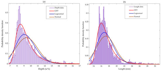
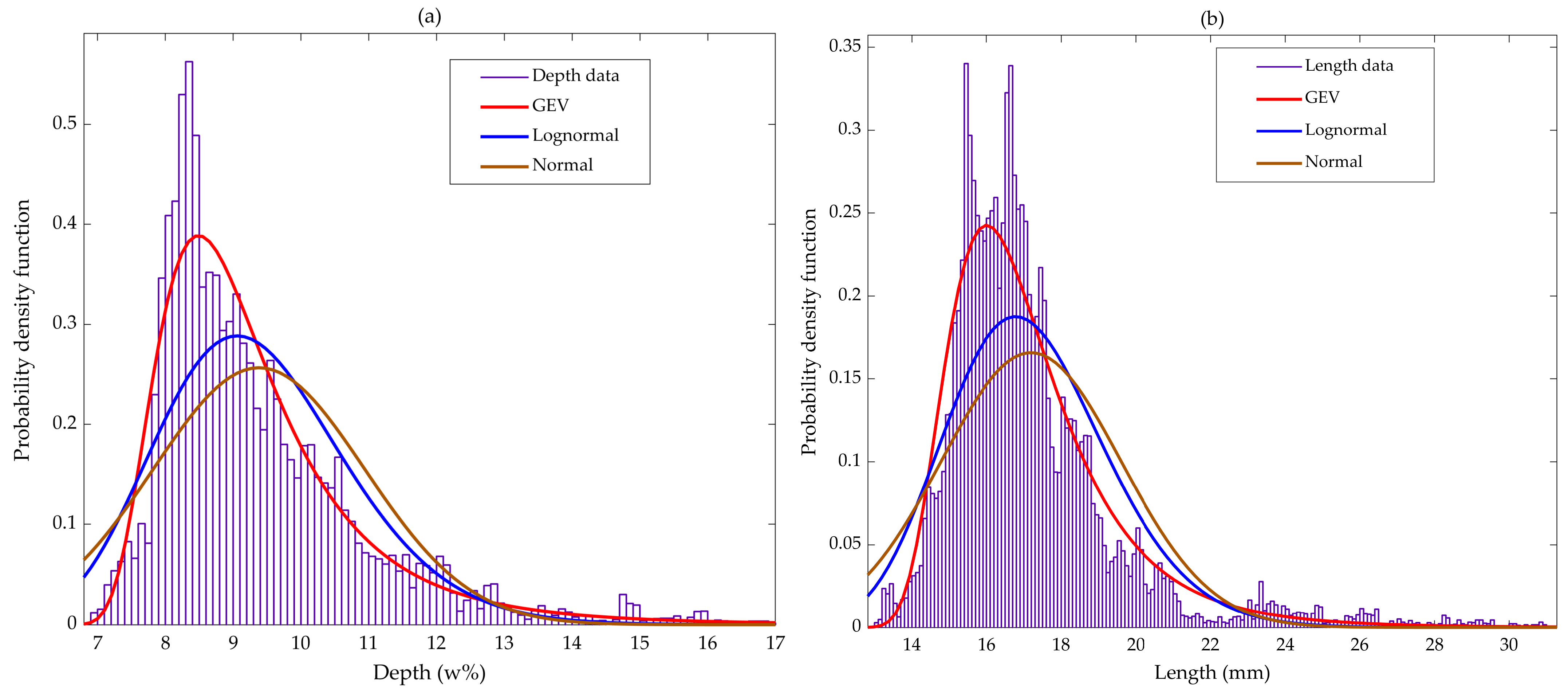
The depth of corrosion defects varies from 10 to 40% ω of the pipeline wall thickness, while the length of defects varies from 15 to 300 mm. The Kolmogorov–Smirnov test is applied to identify the most representative statistical distribution of corrosion parameters. The results indicated that both the depth and length of corrosion defects follow generalized extreme value distributions, as shown in Figure 2.
Figure 2.
Probability density function of corrosion defects: (a) depth and (b) length.
Since only one ILI (In-Line Inspection) measurement is available, the parameters of the inverse Gaussian (IG) process, denoted as IG(), are derived using reference points obtained during the most recent repair. However, an additional ILI measurement is necessary for calibration purposes. The mean growth rate of the defect () is estimated to be 0.2 mm/year. The scale parameter () is calculated using the Maximum Likelihood Estimation (MLE) method, yielding a value of 1.2 mm−1 with a coefficient of variation of 50%. This high CoV indicates significant variability in the corrosion depth growth rate across different pipeline segments.
Regarding defect length, no degradation process was assumed, meaning it is considered constant and equal to the value reported by the ILI tool. While degradation processes that increase corrosion length and width are expected, these parameters are not critical for the failure modes analyzed in this study.
3.2. Identification of the Critical Segments Along the Pipeline
3.2.1. Preliminary Data Analysis
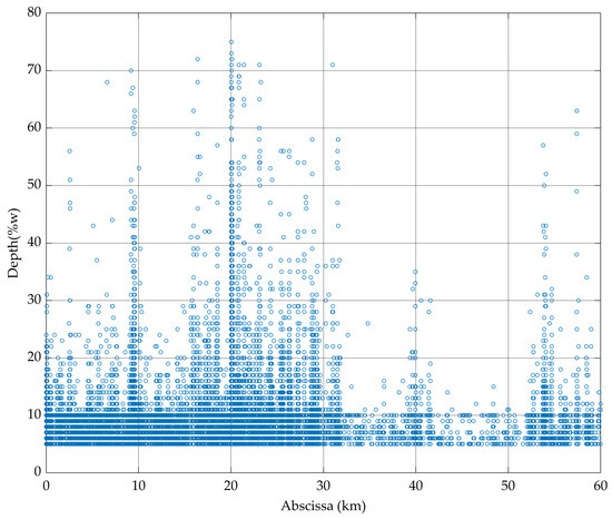
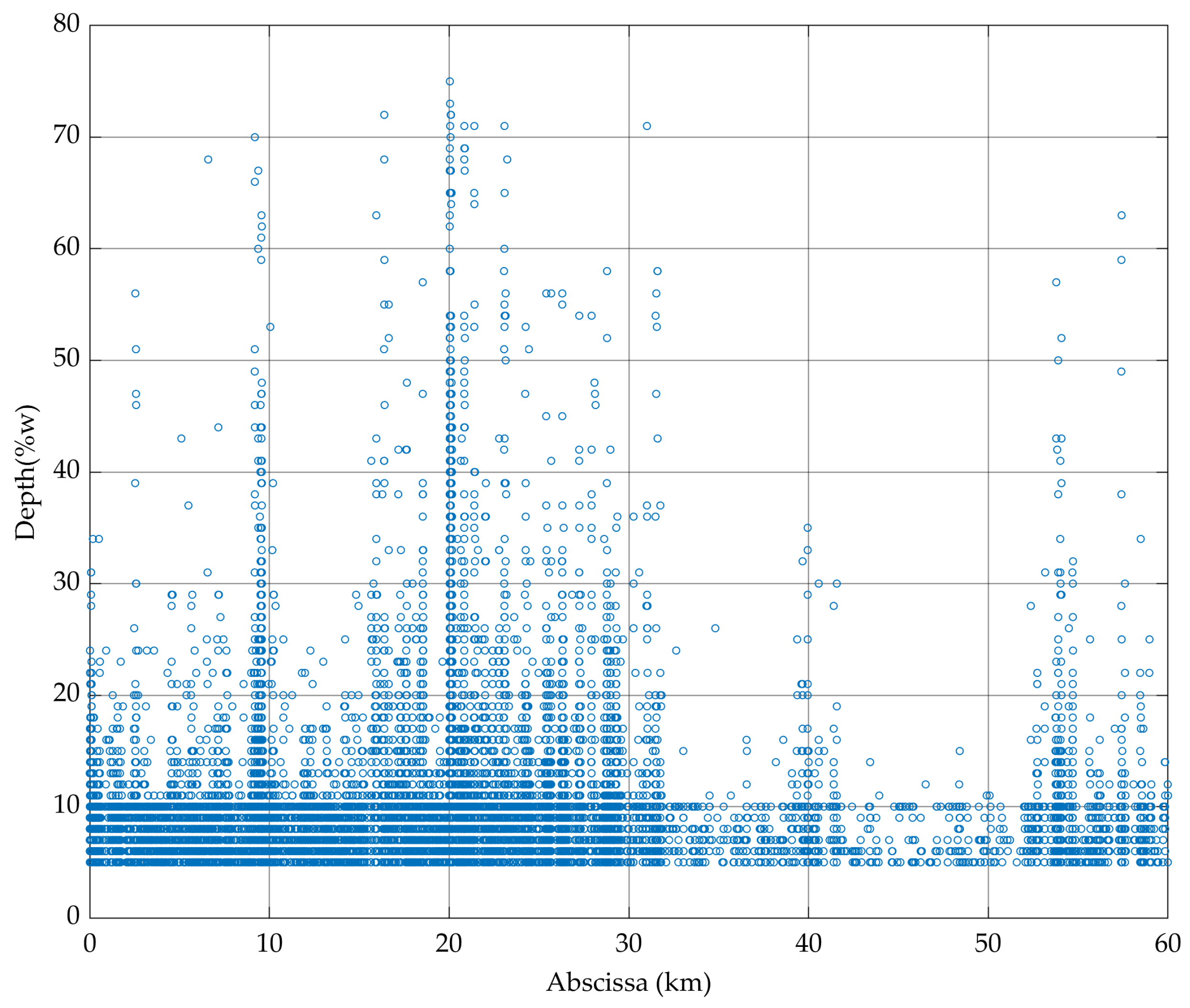
Based on the information obtained by the ILI tool regarding corrosion defects of the outer wall, the dispersion of defect depth along the pipeline abscissa is depicted in Figure 3. We can clearly observe that a high concentration of depth defects is located around 10% ω along the pipeline. Some defects reach 70% ω, which represents a considerable risk of leakage at certain pipeline segments. In terms of the corrosion extent, on the outer wall it was found that the defect depth and length tend to be positively correlated, where a correlation coefficient of was obtained.
Figure 3.
Dispersion of outer wall corrosion depth defects along the pipeline.
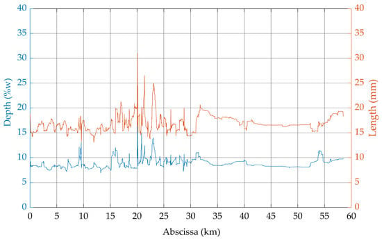
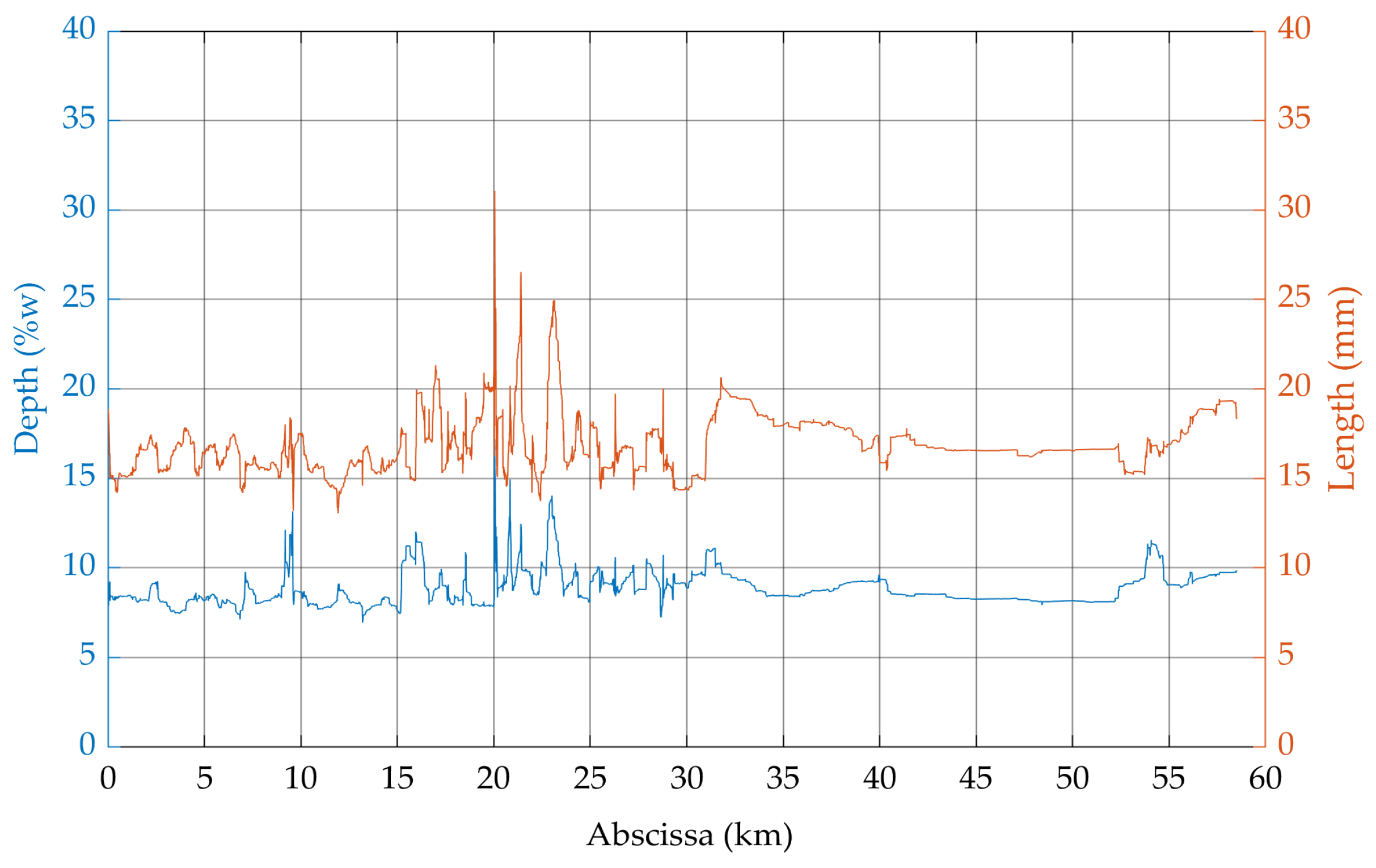
Following the changepoint approach, the defect depth and length measurements from the ILI runs were transformed using the Moving Average Filter. This filter is applied to reduce noise in the input signal. For this purpose, we chose the , where is the set of measurements associated with the length and depth of defects of corrosion. This choice corresponds to smoothing over approximately of the number of measurements. This provides sufficient noise reduction without masking average signal jumps which is useful for the changepoint approach; for more details on the use of the filter, we suggest referring to [17]. The obtained results are presented in Figure 4.
Figure 4.
Filtered measurements of the detected defect along the pipeline.
The results indicate that significant peaks in the mean depth and length of defects are observed around kilometers 9, 16, 20, 21, and 23 along the pipeline’s abscissa. Beyond the 35th kilometer, these measurements exhibit more dispersed patterns, as the number of defects in this section is notably lower compared to the preceding segment. This observation suggests that the environment in this section is less aggressive, leading to reduced corrosion activity. Consequently, it can be inferred that a space-dependent degradation process is active, with varying intensity along the pipeline.
3.2.2. Dynamic Segmentation
Using the filtered corrosion data, dynamic segmentation was performed by identifying optimal changepoints, which correspond to locations where significant changes in defect depth and length patterns were observed. This analysis was conducted using the cpt.mean function in R, (version 4.1.3) as described by Amaya-Gómez et al. [17], and applied within the CROPS framework. A range of penalty values, from = 1 to = 10,000, was considered to ensure robust segmentation.
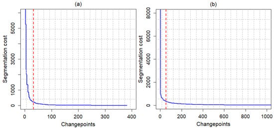
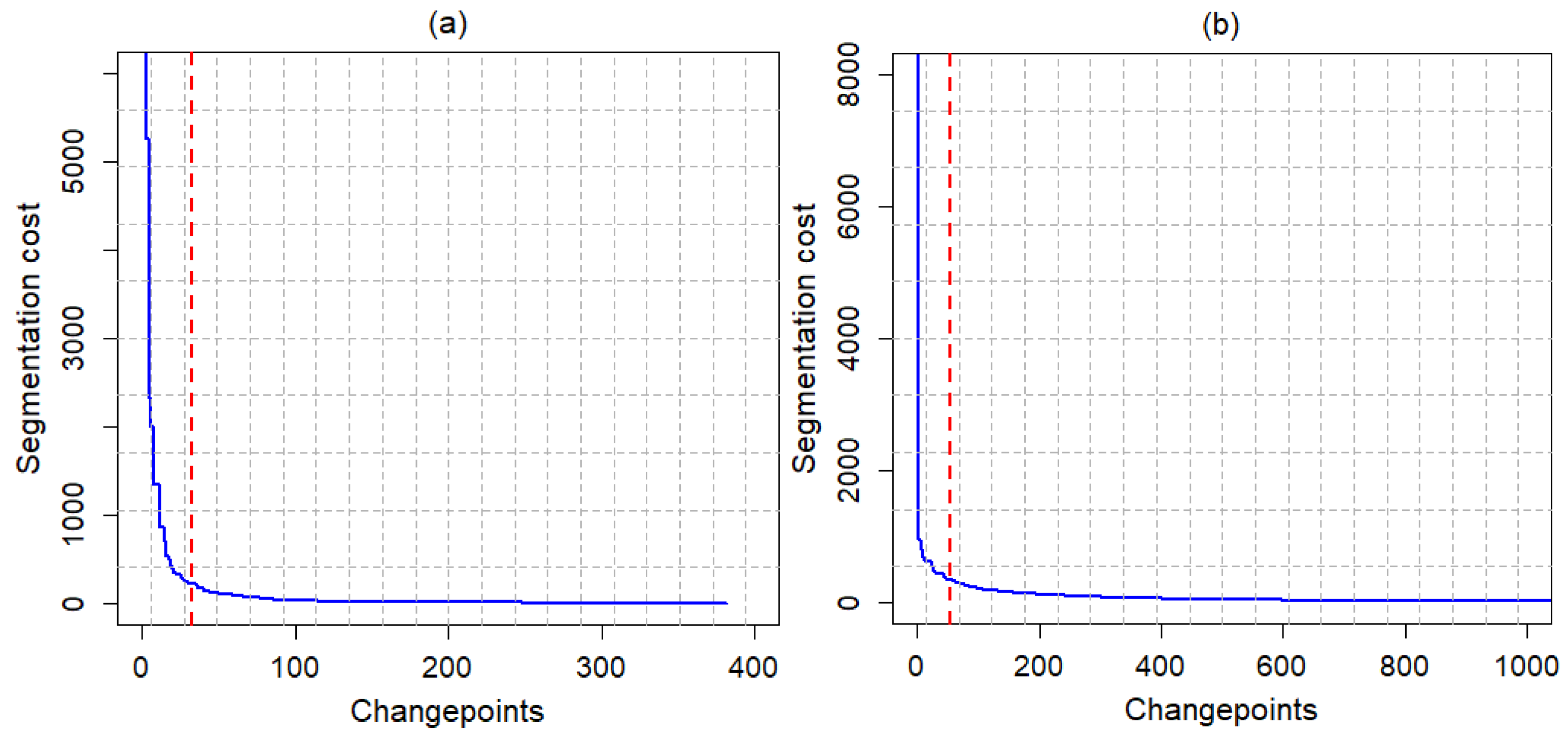
The results for defect depth and length are presented in Figure 5. Overall, the number of changepoints, representing locations where abrupt changes in the filtered depth and length occur, depends on the segmentation cost. Notably, this cost decreases as the number of changepoints increases, reflecting a trade-off between model complexity and fit quality.
Figure 5.
Changepoints vs. segmentation cost for: (a) depth and (b) length defects.
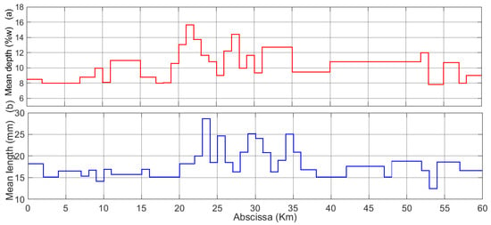
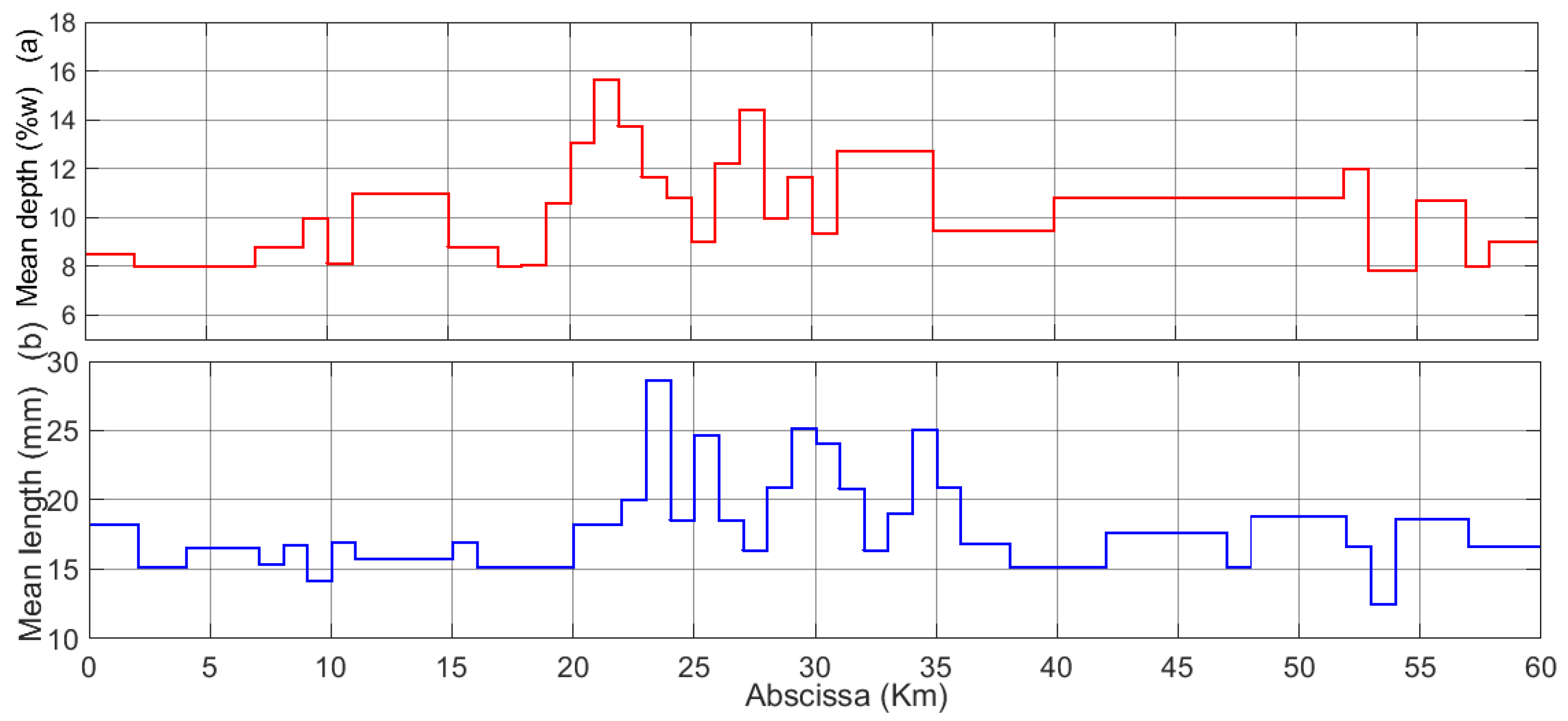
By applying the spline cubic based on the Slmengine function, for approximating the costs, the maximum curvature approach is used to find the optimal changepoints. As depicted in the above figures, it was found that the optimal number of changepoints for depth defects is lower (33) than length (54) (red lines in Figure 5). From the optimal number of changepoints, the segments are identified and their mean and location of depth and length along the pipeline are assessed and represented in Figure 6.
Figure 6.
Mean of (a) depth and (b) length of corrosion defects along the pipeline based on the dynamic segmentation.
The results presented in Figure 6 highlight significant variability in the mean depth of the pipeline segments (Figure 6a), which ranges from 8% to 16% of the pipeline’s outer wall thickness. The segments with the deepest defects are located between 20 km and 35 km. Similarly, the mean defect length also shows considerable variability, ranging from 13 mm to 28 mm, as illustrated in Figure 6b. Notably, the segments with the longest defects are also concentrated in the 20–35 km range. These findings indicate that the section of the pipeline between 20 km and 35 km exhibits higher corrosion aggressiveness compared to other areas. Additionally, it was observed that the depth and length of defects vary across segments. To address this, segments with fewer than 100 defects were merged with adjacent segments to ensure more robust analysis. These spatial results can inform maintenance intervention priorities by identifying critical segments that are at higher risk of leaks or bursts, as indicated by the conditions described in the ILI measurements.
3.2.3. Spatial Identification of Critical Segments Based on a Reliability Approach
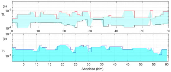
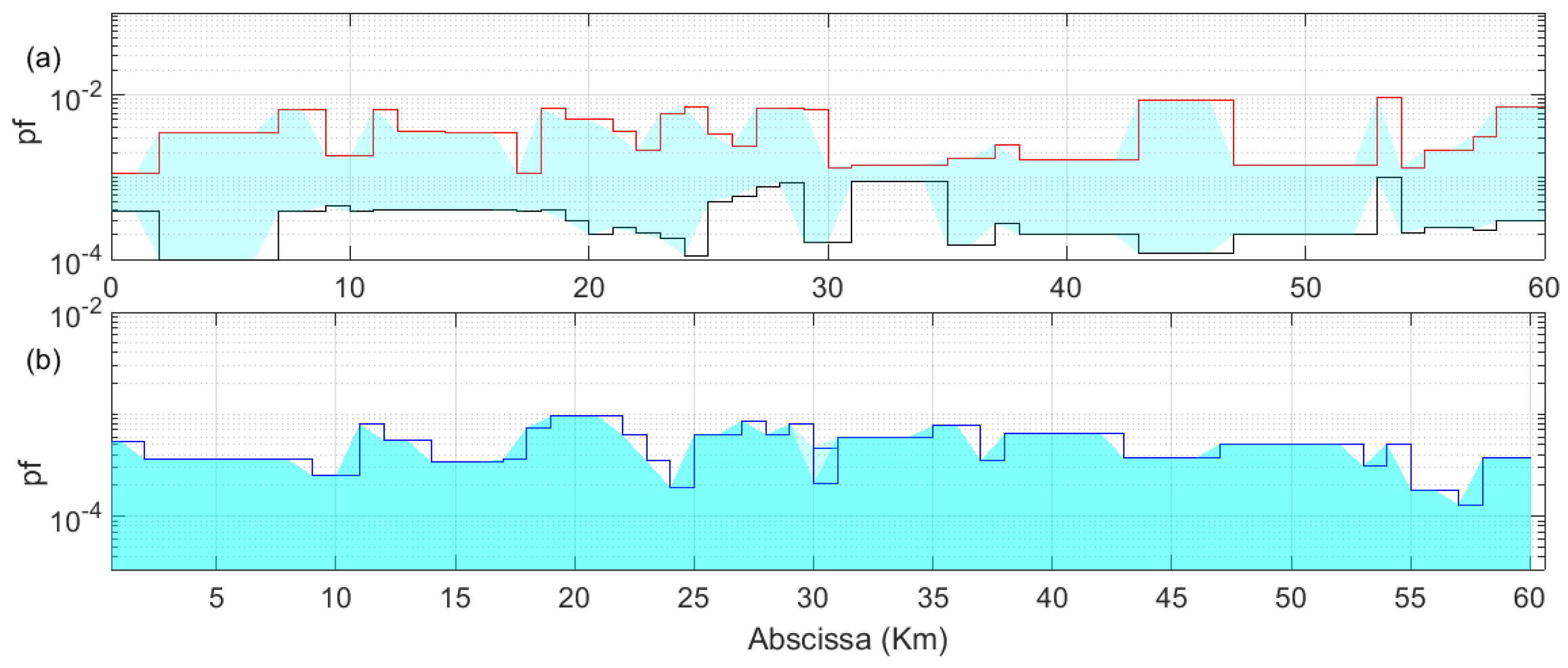
According to the failure criteria for pipeline segments caused by small leaks and bursts, as outlined in Section 2, failure probabilities for segments identified using the changepoint approach were evaluated through 10,000 Monte Carlo simulations for each reported defect (depth and length). Using Equation (7), the failure probabilities for small leaks and bursts in each segment were bounded. The simulation results are presented in Figure 7. The results indicate that the failure probabilities due to small leaks are significantly higher than those caused by bursts. This difference is attributed to the spatio-temporal variability of corrosion defect depth. Additionally, some segments exhibit identical failure probabilities for both failure modes. This similarity can be explained by the fact that these segments are exposed to the same environmental conditions, such as soil aggressiveness, surrounding the pipeline. These findings emphasize the importance of segmentation, which aims to group pipeline sections with similar levels of degradation or reliability. The results obtained here can assist operators in prioritizing maintenance decisions, such as recoating, sleeving, or replacement, for critical segments identified through the changepoint approach. It is important to note that the depth of corrosion defects in pipeline segments evolves stochastically over time. As a result, the reliability of segments and corresponding maintenance actions must be adjusted dynamically to account for these changes.
Figure 7.
Pipeline failure probability based on the changepoint approach: (a) small leaks, and (b) bursts.
3.3. Spatio-Temporal Reliability Assessment
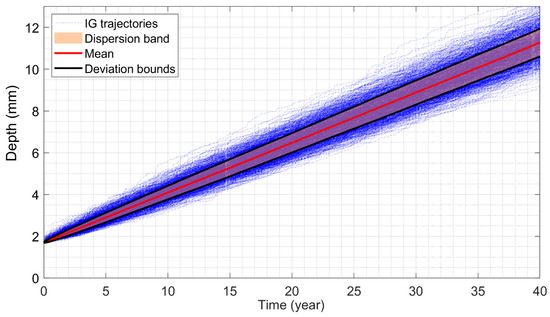
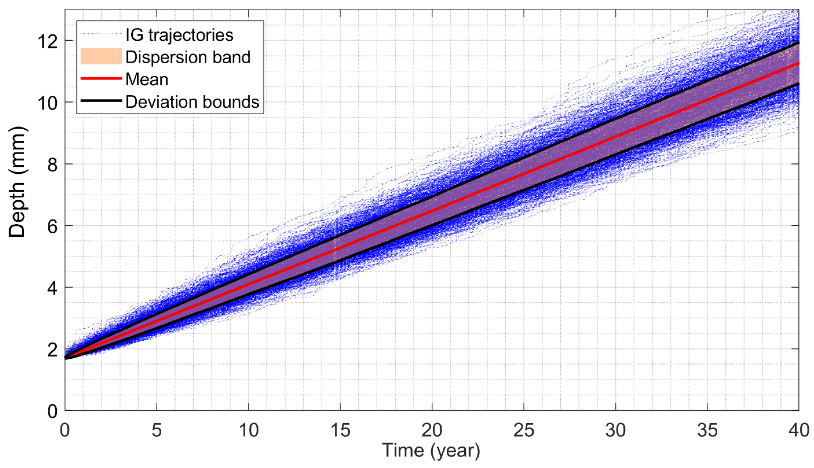
The inverse Gaussian process as described in (Equation (5)) is used for modeling the depth increments of corrosion defects. The mean and shape parameters of the IGP are estimated as described in Section 3.1. Then, Monte Carlo simulations, based on the inverse Gaussian process, were carried out to predict the possible evolution trajectories of a defect depth. The simulation results associated with the maximum corrosion depth, in a given segment, are shown in Figure 8.
Figure 8.
Growth of corrosion depth over time according to the IGP.
In Figure 8, the blue curves represent the trajectories of defect depth, illustrating significant variability that reflects the stochastic nature of the corrosion degradation process. In contrast, the red curve depicts the mean degradation trajectory. The results indicate that on average, after 35 years, the corrosion depth reaches 10 mm, which corresponds to about 80% of the pipeline wall’s thickness. This suggests that a critical threshold for leaks could be reached.
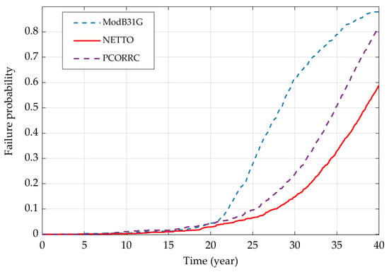
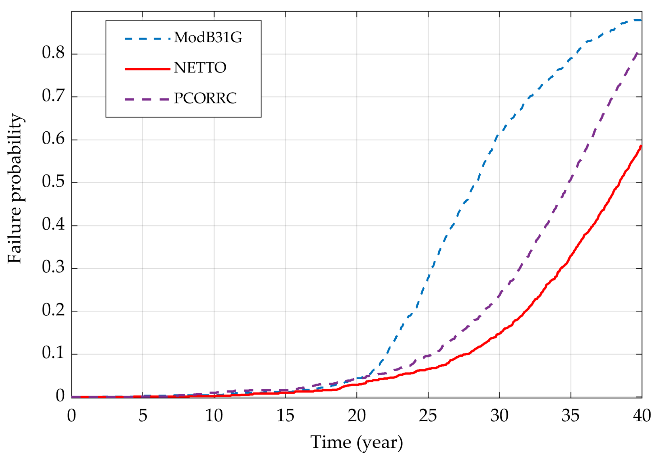
The results obtained using the proposed changepoint approach were utilized to compare burst failure predictions across three models: Netto (see Section 2.2), ModB31G, and PCORRC. For detailed descriptions of the ModB31G and PCORRC models, readers are referred to [38]. Monte Carlo simulations were employed to estimate the burst failure probabilities for each model, and the results are presented in Figure 9. As shown in the figure, the models exhibit similar failure probabilities up to the 20-year mark. However, beyond this point, their predictions diverge. For instance, to reach a failure probability of 0.1, the estimated service life is 22 years for the ModB31G model, 25 years for the PCORRC model, and 27 years for the Netto model. These results indicate that the Netto model provides less conservative predictions compared to the other two models. The findings align with the trends reported by Hasan et al. [38], further validating the choice of the Netto model.
Figure 9.
Comparison of burst model predictions based on the proposed approach.
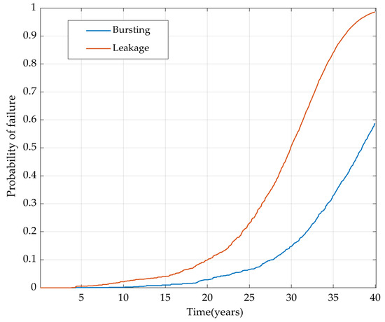
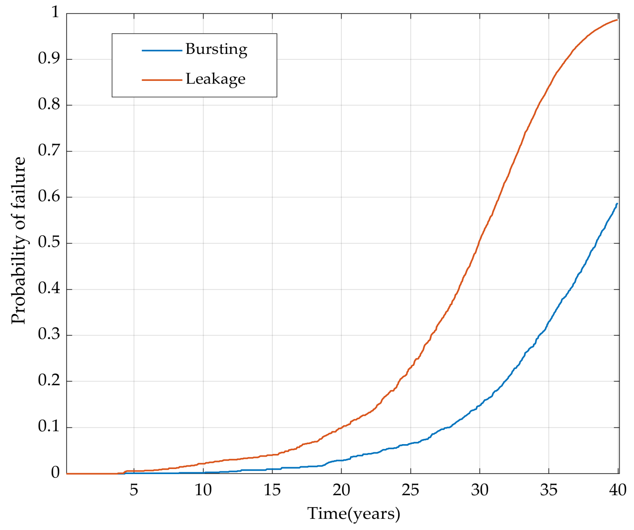
The failure probabilities for two distinct limit states (leakage and bursting) are evaluated for each identified pipeline segment using the changepoint approach over a 40-year forecasting period. As detailed in Section 2.1, the lower bound of Equation (7) is applied, which accounts for the spatial correlation of defects. In this approach, the most critical defect within each segment is used to determine the segment’s failure probability. Subsequently, the overall failure probabilities for the entire pipeline are calculated using a series system reliability framework (see Equation (8)). The results are illustrated in Figure 10. These results incorporate the spatio-temporal variability across the different pipeline segments. It can be observed that the failure probabilities associated with small leaks are higher than those associated with bursts. This highlights the greater likelihood of leakage events compared to bursting failures over the analyzed time horizon.
Figure 10.
Spatio-temporal assessment of pipeline segment’s reliability.
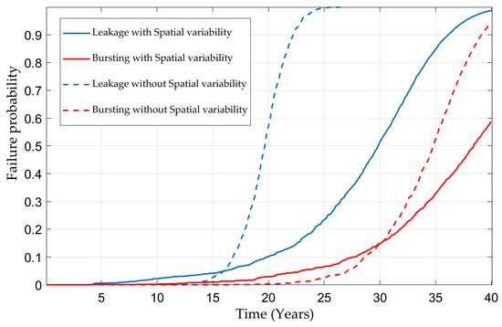
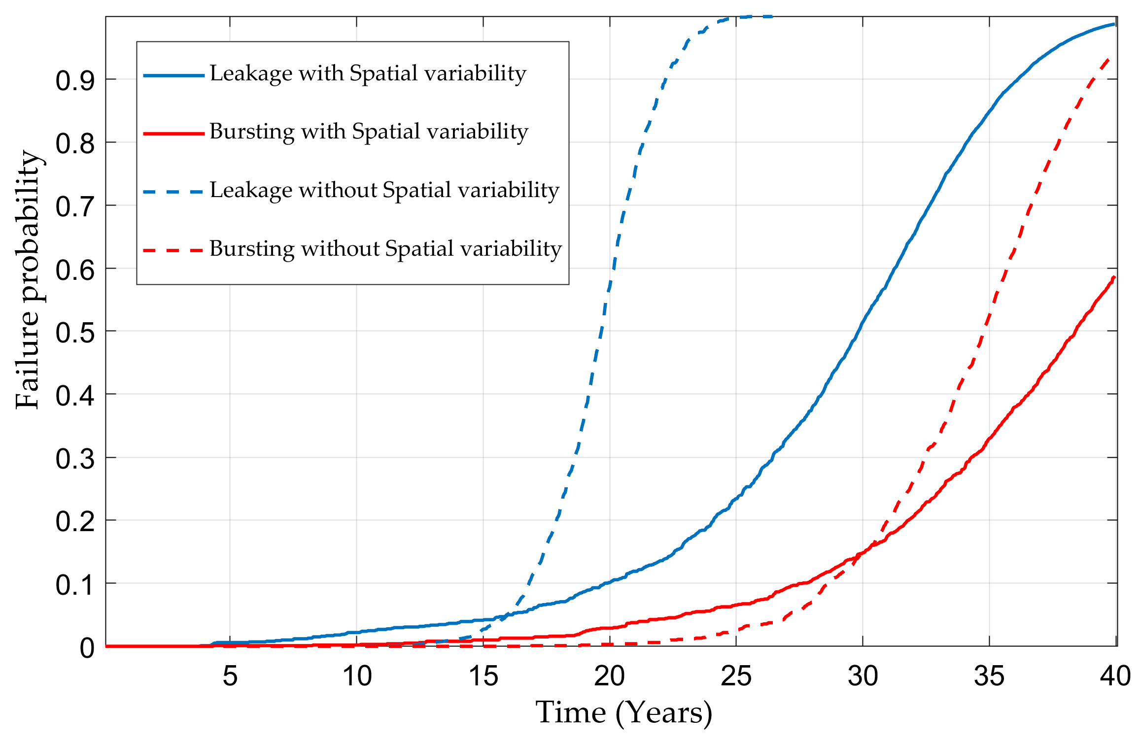
To evaluate the impact of incorporating spatial variability in reliability analysis, an additional assessment was conducted under the assumption of spatially homogeneous degradation (i.e., without spatial variability). The corresponding results and comparisons are presented in Figure 11. These results demonstrate that failure probabilities for leaks and bursts are significantly higher when spatial variability is not considered. This highlights the critical importance of identifying and accounting for spatial heterogeneity, as critical segments are often overlooked under the homogeneous assumption. Moreover, the analysis reveals that leak probabilities are considerably more sensitive to spatial variability than burst probabilities. This is attributed to the direct relationship between the occurrence of leaks and the depth of corrosion. In contrast, the results for bursting failures align with findings reported in [18], further validating the approach. Assuming spatial homogeneity overestimates overall pipeline failure probabilities, which forces operators into premature, unnecessary repairs. Condition-based dynamic segmentation allows operators to target maintenance resources strictly on critical segments without over-maintaining low-risk sections.
Figure 11.
Comparison of the failure probabilities with and without spatial variability.
The overall pipeline failure mode is evaluated as a combined failure, as described in Section 2.4 (Equation (9)). Since these failure events are related, a copula function is used to assess the dependency between them. Various types of copulas (listed in Table 1) are evaluated, and their Akaike Information Criterion values are provided in Table 5. Based on the AIC results, the Clayton copula function is identified as the one providing the best fit and will be used in this study. In this case, the Clayton copula mathematically captures lower-tail dependence. Physically, as corrosion depth progresses, the small leak limit state (80% wall thickness threshold) and the burst limit state simultaneously degrade, creating asymmetric lower-tail clustering of joint failure probabilities that symmetric (Gaussian) or upper-tail (Gumbel) copulas fail to represent.
Table 5.
AIC of different copulas’ functions.
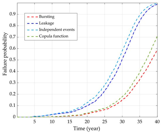
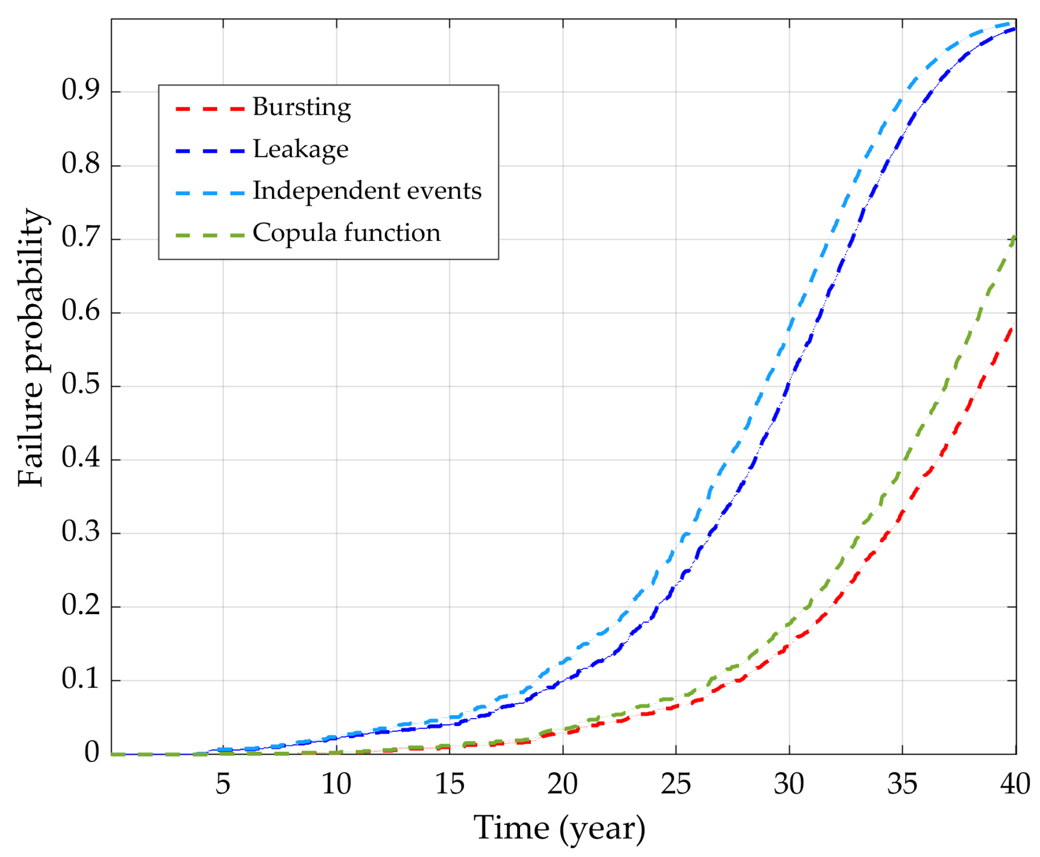
The pipeline failure probabilities under various scenarios and assumptions are presented in Figure 12, comparing leakage and burst failure modes under both dependent and independent assumptions. The results indicate that the highest failure probability occurs when evaluating independent failure events (Equation (10)). Under this independence assumption, there is an overestimation of failure probability which is overall driven by leakage, whereas burst failure represents the lowest probability. Assuming dependence between failure modes (via a copula function) yields a more realistic assessment where failure probabilities are bounded between those of the other failure modes.
Figure 12.
Failure probability of pipeline under different failure modes.
4. Conclusions
Corroded pipelines provide a challenge from both a temporal and spatial point of view for identifying critical segments and planning future interventions (i.e., inspections or repairs). This work presented a probabilistic framework to enhance the reliability assessment of corroded pipelines based on In-Line Inspection measurements. For this purpose, spatial variability was characterized through dynamic segmentation using a changepoint approach and temporal degradation using an inverse Gaussian process for modeling the depth increments. Burst or leak failure criteria are commonly contemplated for reliability purposes separately. However, in this work, a joint failure probability is evaluated by using a copula approach and Monte Carlo simulations.
The main findings of this study can be summarized as follows:
- The ILI-derived corrosion measurements along the pipe’s outer wall exhibit pronounced spatial fluctuations at specific locations, which is consistent with the recognized influence of local soil conditions on external corrosion initiation and propagation. The proposed changepoint approach effectively captured this spatial heterogeneity, enabling the segmentation of the pipeline into homogeneous zones and the identification of critical segments according to their reliability level. This segmentation provides a physically meaningful basis for prioritizing inspection and maintenance efforts.
- The copula-based framework successfully captured the statistical dependence between leakage and bursting failure scenarios, yielding a more realistic estimate of their joint failure probability than the conventional independence assumption. By explicitly modeling the dependence structure between failure modes, the approach reflects the shared underlying deterioration and loading mechanisms driving both scenarios.
- The results demonstrated that disregarding spatial variability leads to an overestimation of failure probabilities. Such overestimation may trigger unnecessary or ill-targeted maintenance interventions, resulting in suboptimal allocation of limited integrity-management resources.
In terms of future perspectives, the proposed spatio-temporal reliability assessment can be integrated into a decision-making framework to optimize long-term pipeline inspection schedules and select targeted interventions. In this regard, a cost model based on renewal theory can be contemplated. To address current data limitations and model assumptions, subsequent work could incorporate multiple consecutive In-Line Inspection datasets to achieve a more precise parameter calibration for the inverse Gaussian degradation process. Furthermore, while defect length was assumed constant because depth is the primary contributor to both small leak and burst limit states, future modeling could expand to capture multi-dimensional, time-dependent defect growth by evaluating length and width progression alongside depth over time. The methodology can also be extended considering the analysis from both the outer and inner walls of the pipeline.
Artificial intelligence offers a very promising alternative for pipeline condition assessment, as data-driven models can learn complex relationships between inspection signals and pipe deterioration. In particular, artificial neural networks have already demonstrated strong potential for trenchless water pipe condition assessment [47], suggesting that these frameworks could significantly improve the accuracy, speed, and cost-effectiveness of pipeline condition evaluation.
Author Contributions
Conceptualization, H.B., R.L., R.A.-G. and E.B.-A.; Writing—Original Draft, H.B.; Software, H.B.; Methodology, H.B., R.L., R.A.-G. and E.B.-A.; Formal Analysis, H.B.; Supervision, R.L., R.A.-G. and E.B.-A.; Validation, R.L., R.A.-G. and E.B.-A.; Writing—Review and Editing, R.L., R.A.-G. and E.B.-A. All authors have read and agreed to the published version of the manuscript.
Funding
This research received no external funding.
Data Availability Statement
The data presented in our study comes from ILI and concerns corrosion defects in an underground pipeline. For confidentiality reasons, the location of the pipeline and this data are not disclosed.
Conflicts of Interest
The authors declare no conflicts of interest.
Abbreviations
| ILI | In-Line inspection |
| CROPS | Changepoints for a Range of Penalties |
| Wall thickness | |
| Burst pressure | |
| Operating pressure | |
| Diameter | |
| Time | |
| Yield strength | |
| Joint probability density function | |
| MCS | Monte Carlo Simulation |
| FORM | First Order Reliability Method |
| SORM | Second Order Reliability Method |
| Reliability index | |
| Standard normal distribution function | |
| Small leak limit state | |
| Burst limit state | |
| Probability of failure in a segment | |
| Pipeline failure probability | |
| Number of segments | |
| Length of corrosion at time | |
| Initial depth of corrosion in segment | |
| Depth of corrosion in segment at time | |
| Function of performance | |
| Correlation matrix | |
| Uniform marginal of the small leak | |
| Uniform marginal of the burst | |
| Inverse Gaussian process | |
| Mean parameter | |
| Shape parameter | |
| Number of defects | |
| Indicator function | |
| Number of simulations | |
| MLE | Maximum Likelihood Estimation |
| CSA | Canadian Standards Association |
| LHS | Latin Hypercube Sampling |
References
- Amaya-Gómez, R.; Bastidas-Arteaga, E.; Sánchez-Silva, M.; Schoefs, F.; Muñoz, F. Corrosion and Reliability Assessment of Inspected Pipelines; Springer International Publishing: Cham, Switzerland, 2024. [Google Scholar]
- Amaya-Gómez, R.; Bastidas-Arteaga, E.; Muñoz, F.; Sanchez-Silva, M. Statistical Soil Characterization of an Underground Corroded Pipeline Using In-Line Inspections. Metals 2021, 11, 292. [Google Scholar] [CrossRef] [Scilit]
- Zhang, S.; Zhou, W. Cost-Based Optimal Maintenance Decisions for Corroding Natural Gas Pipelines Based on Stochastic Degradation Models. Eng. Struct. 2014, 74, 74–85. [Google Scholar] [CrossRef] [Scilit]
- POF (Pipeline Operators Forum). Specifications and Requirements for Intelligent Pig Inspection of Pipelines; POF: Vancouver, BC, Canada, 2009. [Google Scholar]
- NACE SP0169-2007; Control of External Corrosion on Underground or Submerged Metallic Piping Systems. National Association of Corrosion Engineers: Houston, TX, USA, 2007.
- Pandey, M.D.; Van Noortwijk, J.M. Gamma Process Model for Time-Dependent Structural Reliability Analysis. In Bridge Maintenance, Safety, Management and Cost, Proceedings of the Second International Conference on Bridge Maintenance, Safety and Management (IABMAS), Kyoto, Japan, 18–22 October 2004; CRC Press: Boca Raton, FL, USA, 2004; pp. 18–22. [Google Scholar]
- Vanaei, H.R.; Eslami, A.; Egbewande, A. A Review on Pipeline Corrosion, in-Line Inspection (ILI), and Corrosion Growth Rate Models. Int. J. Press. Vessel. Pip. 2017, 149, 43–54. [Google Scholar] [CrossRef] [Scilit]
- Bouledroua, O.; Zelmati, D.; Hassani, M. Inspections, Statistical and Reliability Assessment Study of Corroded Pipeline. Eng. Fail. Anal. 2019, 100, 1–10. [Google Scholar] [CrossRef] [Scilit]
- Ait Mokhtar, E.H.; Chateauneuf, A.; Laggoune, R. Bayesian Approach for the Reliability Assessment of Corroded Interdependent Pipe Networks. Int. J. Press. Vessel. Pip. 2016, 148, 46–58. [Google Scholar] [CrossRef] [Scilit]
- Gong, C.; Zhou, W. Multi-Objective Maintenance Strategy for in-Service Corroding Pipelines Using Genetic Algorithms. Struct. Infrastruct. Eng. 2018, 14, 1561–1571. [Google Scholar] [CrossRef] [Scilit]
- Ossai, C.I. Finite Element Modelling and Retained Life Estimation of Corroded Pipelines in Consideration of Burst Pressures—A Fractural Mechanics Approach. Infrastructures 2017, 2, 15. [Google Scholar] [CrossRef] [Scilit]
- Caleyo, F.; Velázquez, J.C.; Valor, A.; Hallen, J.M. Probability Distribution of Pitting Corrosion Depth and Rate in Underground Pipelines: A Monte Carlo Study. Corros. Sci. 2009, 51, 1925–1934. [Google Scholar] [CrossRef] [Scilit]
- Liu, X.; Zheng, J.; Fu, J.; Nie, Z.; Chen, G. Optimal Inspection Planning of Corroded Pipelines Using BN and GA. J. Pet. Sci. Eng. 2018, 163, 546–555. [Google Scholar] [CrossRef] [Scilit]
- Zhang, S.; Zhou, W.; Qin, H. Inverse Gaussian Process-Based Corrosion Growth Model for Energy Pipelines Considering the Sizing Error in Inspection Data. Corros. Sci. 2013, 73, 309–320. [Google Scholar] [CrossRef] [Scilit]
- Li, X.; Liu, Y.; Zhang, R.; Zhang, N. Probabilistic Failure Assessment of Oil and Gas Gathering Pipelines Using Machine Learning Approach. Reliab. Eng. Syst. Saf. 2025, 256, 110747. [Google Scholar] [CrossRef] [Scilit]
- Amaya-Gómez, R.; Sánchez-Silva, M.; Muñoz, F. Integrity Assessment of Corroded Pipelines Using Dynamic Segmentation and Clustering. Process Saf. Environ. Prot. 2019, 128, 284–294. [Google Scholar] [CrossRef] [Scilit]
- Amaya-Gómez, R.; Bastidas-Arteaga, E.; Schoefs, F.; Munoz, F.; Sanchez-Silva, M. A Condition-Based Dynamic Segmentation of Large Systems Using a Changepoints Algorithm: A Corroding Pipeline Case. Struct. Saf. 2020, 84, 101912. [Google Scholar] [CrossRef] [Scilit]
- Sahraoui, Y.; Chateauneuf, A. The Effects of Spatial Variability of the Aggressiveness of Soil on System Reliability of Corroding Underground Pipelines. Int. J. Press. Vessel. Pip. 2016, 146, 188–197. [Google Scholar] [CrossRef] [Scilit]
- Xiao, R.; Zayed, T.; Meguid, M.A.; Sushama, L. Reliability Analysis of Gas Pipelines Considering Spatial and Temporal Corrosion Variability. J. Pipeline Sci. Eng. 2025, 5, 100256. [Google Scholar] [CrossRef] [Scilit]
- Meneses-Gelves, J.A.; Sánchez-Silva, M.; Amaya-Gómez, R. Spatial Variability Analysis of Corroded Pipelines Using Random Fields: Degradation and Reliability Assessment. Reliab. Eng. Syst. Saf. 2026, 272, 112519. [Google Scholar] [CrossRef] [Scilit]
- CSA Z662-07; Limit State Equation for Burst of Large Leaks and Rupture for Corrosion Defect. Canadian Standards Association: Toronto, ON, USA, 2007.
- Zhou, W.; Hong, H.P.; Zhang, S. Impact of Dependent Stochastic Defect Growth on System Reliability of Corroding Pipelines. Int. J. Press. Vessel. Pip. 2012, 96, 68–77. [Google Scholar] [CrossRef] [Scilit]
- Zhou, W.; Xiang, W.; Hong, H.-P. Sensitivity of System Reliability of Corroding Pipelines to Modeling of Stochastic Growth of Corrosion Defects. Reliab. Eng. Syst. Saf. 2017, 167, 428–438. [Google Scholar] [CrossRef] [Scilit]
- Nelsen, R.B. An Introduction to Copulas; Springer Science & Business Media: New York, NY, USA, 2006. [Google Scholar]
- Wang, Y.; Xie, M.; Su, C. Multi-Objective Maintenance Strategy for Corroded Pipelines Considering the Correlation of Different Failure Modes. Reliab. Eng. Syst. Saf. 2024, 243, 109894. [Google Scholar] [CrossRef] [Scilit]
- Wang, W.; Wang, Y.; Zhang, B.; Shi, W.; Li, C.-Q. Failure Prediction of Buried Pipe Network with Multiple Failure Modes and Spatial Randomness of Corrosion. Int. J. Press. Vessel. Pip. 2021, 191, 104367. [Google Scholar] [CrossRef] [Scilit]
- Wu, W.; Shen, Z.; Tian, Y. Pipeline walking under spatially variable seabed resistance: An analytical framework with random fields. Mar. Struct. 2027, 111, 104209. [Google Scholar] [CrossRef] [Scilit]
- De Leon, D.; Macías, O.F. Effect of Spatial Correlation on the Failure Probability of Pipelines under Corrosion. Int. J. Press. Vessel. Pip. 2005, 82, 123–128. [Google Scholar] [CrossRef] [Scilit]
- Killick, R.; Fearnhead, P.; Eckley, I.A. Optimal Detection of Changepoints with a Linear Computational Cost. J. Am. Stat. Assoc. 2012, 107, 1590–1598. [Google Scholar] [CrossRef] [Scilit]
- Haynes, K.; Eckley, I.A.; Fearnhead, P. Efficient Penalty Search for Multiple Changepoint Problems. arXiv 2014, arXiv:1412.3617. [Google Scholar]
- Zhu, X.-K. Burst Pressure Models and Validations for Thick-Walled Pipelines Containing Corrosion Defects. J. Pipeline Sci. Eng. 2025, 5, 100301. [Google Scholar] [CrossRef] [Scilit]
- Amaya-Gómez, R.; Sánchez-Silva, M.; Bastidas-Arteaga, E.; Schoefs, F.; Muñoz, F. Reliability Assessments of Corroded Pipelines Based on Internal Pressure—A Review. Eng. Fail. Anal. 2019, 98, 190–214. [Google Scholar] [CrossRef] [Scilit]
- ASME B31G; Manual for Determining the Remaining Strength of Corroded Pipelines. American Society of Mechanical Engineers: New York, NY, USA, 2009.
- Netto, T.A.; Ferraz, U.S.; Estefen, S.F. The Effect of Corrosion Defects on the Burst Pressure of Pipelines. J. Constr. Steel Res. 2005, 61, 1185–1204. [Google Scholar] [CrossRef] [Scilit]
- Ma, B.; Shuai, J.; Liu, D.; Xu, K. Assessment on Failure Pressure of High Strength Pipeline with Corrosion Defects. Eng. Fail. Anal. 2013, 32, 209–219. [Google Scholar] [CrossRef] [Scilit]
- Development of an Alternative Criterion for Residual Strength of Corrosion Defects in Moderate-to High-Toughness Pipe|IPC|ASME Digital Collection. Available online: https://asmedigitalcollection.asme.org/IPC/proceedings/IPC2000/40252/V002T06A012/266139 (accessed on 13 September 2026).
- Chen, Y.; Zhang, H.; Zhang, J.; Li, X.; Zhou, J. Failure Analysis of High Strength Pipeline with Single and Multiple Corrosions. Mater. Des. 2015, 67, 552–557. [Google Scholar] [CrossRef] [Scilit]
- Hasan, S.; Khan, F.; Kenny, S. Probability Assessment of Burst Limit State Due to Internal Corrosion. Int. J. Press. Vessel. Pip. 2012, 89, 48–58. [Google Scholar] [CrossRef] [Scilit]
- Caleyo, F.; Gonzalez, J.L.; Hallen, J.M. A Study on the Reliability Assessment Methodology for Pipelines with Active Corrosion Defects. Int. J. Press. Vessel. Pip. 2002, 79, 77–86. [Google Scholar] [CrossRef] [Scilit]
- Sánchez-Silva, M.; Klutke, G.-A. Reliability and Life-Cycle Analysis of Deteriorating Systems; Springer Series in Reliability Engineering; Springer International Publishing: Cham, Switzerland, 2016. [Google Scholar]
- Zeng, W.; Han, Y.; Tian, X.; Zhao, J. Reliability Modelling and Assessment of Subsea Oil and Gas Pipelines Considering Competing Failures Caused by Dropped Object Impact and Corrosion Degradation. Appl. Ocean Res. 2025, 164, 104783. [Google Scholar] [CrossRef] [Scilit]
- Abyani, M.; Bahaari, M.R. A Comparative Reliability Study of Corroded Pipelines Based on Monte Carlo Simulation and Latin Hypercube Sampling Methods. Int. J. Press. Vessel. Pip. 2020, 181, 104079. [Google Scholar] [CrossRef] [Scilit]
- Durante, F.; Fernández-Sánchez, J.; Sempi, C. A Topological Proof of Sklar’s Theorem. Appl. Math. Lett. 2013, 26, 945–948. [Google Scholar] [CrossRef] [Scilit]
- Zhang, P.; Su, L.; Qin, G.; Kong, X.; Peng, Y. Failure Probability of Corroded Pipeline Considering the Correlation of Random Variables. Eng. Fail. Anal. 2019, 99, 34–45. [Google Scholar] [CrossRef] [Scilit]
- Cherubini, U.; Luciano, E.; Vecchiato, W. Copula Methods in Finance; John Wiley & Sons: Chichester, UK, 2004. [Google Scholar]
- Boufkhed, H.; Laggoune, R.; Bastidas-Arteaga, E. Optimization of the Maintenance of Pipelines Subject to Corrosion Defects. In Proceedings of the 2024 International Conference of the African Federation of Operational Research Societies (AFROS); IEEE: Tlemcen, Algeria, 2024; pp. 1–5. [Google Scholar]
- Geem, Z.W.; Tseng, C.-L.; Kim, J.; Bae, C. Trenchless Water Pipe Condition Assessment Using Artificial Neural Network. In Pipelines 2007: Advances and Experiences with Trenchless Pipeline Projects—Proceedings of the ASCE International Conference on Pipeline Engineering and Construction; American Society of Civil Engineers (ASCE): Reston, VA, USA, 2007; pp. 1–9. [Google Scholar] [CrossRef] [Scilit]

Disclaimer/Publisher’s Note: The statements, opinions and data contained in all publications are solely those of the individual author(s) and contributor(s) and not of MDPI and/or the editor(s). MDPI and/or the editor(s) disclaim responsibility for any injury to people or property resulting from any ideas, methods, instructions or products referred to in the content. |
© 2026 by the authors. Licensee MDPI, Basel, Switzerland. This article is an open access article distributed under the terms and conditions of the Creative Commons Attribution (CC BY) license.