


Highlights
What are the main findings?
- MeteoFormer achieves the lowest MAE among eleven models on the Jena dataset and performance statistically comparable to Crossformer on the Beijing dataset for 24 h meteorological forecasting.
- Built-in attention is not a faithful explanation of MeteoFormer’s predictions: variable-attention fidelity is indistinguishable from zero, while temporal attention remains nearly uniform despite the model’s strong reliance on the most recent 16 h.
What are the implications of the main findings?
- Attention weights should not be interpreted directly as feature importance without quantitative validation against independent attribution and perturbation-based methods.
- Improving forecasting accuracy can compromise the faithfulness of built-in explanations, highlighting the need to evaluate predictive performance and explanation reliability separately when developing meteorological decision-support systems.
Abstract
Built-in attention is often presented as a free explanation of what a forecasting transformer relies on, but the claim is rarely tested. We test it on MeteoFormer, a patch-based transformer with single-head variable and temporal attention that forecasts four weather variables 24 h ahead from 96 h of hourly input on the Jena and Beijing PRSA datasets. Against ten baselines trained under one protocol with five seeds, MeteoFormer has the lowest mean absolute error on Jena (3.025 against 3.107 for Crossformer, Diebold–Mariano p < 0.05 against every baseline after Holm correction) and is level with Crossformer on Beijing (4.151 against 4.138, p = 0.72), while Crossformer has the lower squared error, a difference traced to humidity. The model depends heavily on the latest observations: losing the last 16 h raises its Jena error by 73% and drops it from first to sixth place. The explanation claim fails. The fidelity of the variable attention does not differ from zero (0.012 on Jena, 0.046 on Beijing), far below SHAP on the same model; the temporal attention is almost uniform although the forecast depends mainly on the last 16 h; and the configuration selected for accuracy has the least faithful attention (0.012 against 0.181 with instance normalization, p = 0.001), but the more faithful configuration is less accurate (Jena MAE 3.195 against 3.025) and its attention remains below SHAP.
1. Introduction
Weather forecasts underlie many consequential decisions: a fruit grower deciding whether to irrigate overnight to protect a crop from frost, a grid operator balancing solar and wind supply ahead of a cold front, and an airport deciding whether to pre-treat its runways before the front arrives. In each case, there is an asymmetric cost of acting on a wrong forecast, and no cost of not acting on an unexplained forecast: if a forecaster can not distinguish between a genuine signal and a spurious one, such as a correlation with time of day, they have good reason to doubt the evidence of the forecast model, even if its performance on held-out data is impressive. Interpretability is thus not only a cosmetic feature of a weather forecast, but is also closely related to usability in a decision-support system.
Transformer architectures have transformed multivariate time-series forecasting over the past five years, and the evolution of this field offers a useful case study. Informer [1] used sparse self-attention to make long-horizon transformer forecasting tractable. Autoformer [2] and its frequency-domain counterpart FEDformer [3] disagreed on using raw attention as the right inductive bias and used trend-seasonal decomposition and autocorrelation instead. In turn, much of the previous architectural complexity was found to be redundant when the input is tokenized as overlapping patches instead of individual time-steps, as in PatchTST [4], while the opposite approach was taken by iTransformer [5] and Crossformer [6], which explicitly encouraged cross-variable dependence rather than considering attention only along time. Beneath all these, DLinear [7] produced a less comfortable, but nonetheless important, outcome: a single linear layer per channel with no special effort won or tied to most of the transformer variants listed above on several standard benchmarks. Because of that result, the core question of the field, rather than “how do we make a better transformer,” became “what, if anything, is a transformer really offering us?” For this reason, we include DLinear with all of the other baselines rather than as a footnote.
Of the architectures that ask why a model made a given forecast, very little of this work has been combined with the patch-based and cross-dimension-attention methods discussed above, and the few that do (most notably Temporal Fusion Transformer [8], which fuses the recurrent encoder with variable selection and multi-head attention blocks) predate these two breakthroughs and have never been evaluated on a modern, patch-based, high-accuracy backbone. Some of this gap is filled post hoc: SHAP [9] and its time-series variants (TimeSHAP [10], WindowSHAP [11] and ShapTime [12]) can be used with any trained model; attention rollout [13] can output a summary of the attention that is performed by a transformer. However, there are two costs of post hoc explanation that are easy to overlook. The first is a computational challenge: SHAP-style attribution requires lots of forward passes for each prediction, and is not easily scalable for operational, always-on forecasting. The second is more basic: the raw attention weights, the cheapest information that can be read from a trained transformer, are not necessarily a good indicator of feature importance [14]. That critique started a debate that was further elaborated by Bibal et al. [15], and whose practical consequence is that attention can be used to get a faithful explanation, but not just by reading off what a standard multi-head layer is producing; it must be single-head, explicitly regularized, and be checked against some independent method.
MeteoFormer is built around this cheap source of explanation. A single-head variable-attention layer, not multi-head, for the reason above, generates one distribution of importance per forecasting target, and one entropy penalty on that distribution is directly included in the training loss, so the resulting explanation is not diffuse, but sparse, and is an objective of the training process, not a post-training computation. A second, equally cheap reading is the learned pooling query over patches, which indicates the temporal importance of each input patch and is compared with attention rollout [13] over the encoder’s own layers. Because the model’s built-in explanation is free at inference time, it would be valuable if it were faithful, and this paper tests whether it is, against SHAP and occlusion computed on the same model and on ten baselines under identical conditions.
The contributions are the following. First, MeteoFormer, a patch-based transformer with a multi-scale dilated encoder, single-head variable and temporal attention, an adaptive fusion gate and an auxiliary frost-event head, has the lowest mean absolute error among eleven models on Jena and is level with the strongest baseline on Beijing, with significance established by Diebold–Mariano tests with Holm correction, and it is the most accurate model for temperature on both datasets. Second, we benchmark explanation fidelity for all eleven models on equal budgets and show that the built-in attention is not a faithful explanation: its fidelity is indistinguishable from zero, it is unstable across seeds, and on the time axis it is almost uniform, while occlusion shows that the forecast depends mainly on the last 16 h. Third, we identify a trade-off between accuracy and faithfulness: removing reversible instance normalization, the choice made by the validation loss, gives the model its accuracy and also makes its attention least faithful, and we explain the accuracy side of this effect; across eight configurations of normalization and entropy weight, the reported one, the most accurate on Jena, has the least faithful attention on both datasets, whereas the more faithful configurations are less accurate and still fall short of SHAP. Fourth, we report the limits of the model as openly as its strengths, including its larger squared error on humidity, its sensitivity to an outage of the most recent observations, its transfer to eleven unseen stations and the effect of window length.
2. Related Work
2.1. Transformer-Based Forecasters: From Efficiency to Simplicity
Transformer forecasters have developed through a series of corrections to one another [16,17]. Informer [1] introduced ProbSparse attention to cut the quadratic cost of self-attention and make long horizons tractable. Autoformer [2] then argued that sparse pointwise attention handles long seasonal structure badly, and replaced it with series decomposition and autocorrelation; FEDformer [3] moved the same idea into the frequency domain. The next change was in what counts as a token. PatchTST [4] splits every channel into overlapping patches, borrowing from vision transformers, and gained accuracy and speed over the decomposition models. iTransformer [5] goes the other way and embeds the whole series of each variable as one token, so that attention runs across variables. Crossformer [6] keeps patch-like segments and adds an explicit cross-dimension stage. TimesNet [18] folds the series into 2-D tensors so that ordinary 2-D convolutions can pick up variation within and between periods, and TimeMixer [19] mixes information across several temporal resolutions, which is also the idea behind the dilated multi-scale block of MeteoFormer (Section 3.2.2; see also [20]). Stationarity is the third point of friction. Non-stationary Transformers [21] showed that normalizing away the changing statistics of a series can remove information a transformer needs, and reversible instance normalization (RevIN) [22] made the normalization invertible. We come back to this in Section 5.3, because it turns out to drive the trade-off studied here.
Simple models set the bar for evidence. DLinear [7] showed that one linear layer per channel matches or beats many of these transformers on standard benchmarks, and TSMixer [23] reached similar accuracy with an MLP that alternates between the time and feature axes. A new architecture, ours included, therefore has to be compared with such models under one protocol. Open suites such as the Time-Series-Library [24], whose implementations we use for the baselines, make that comparison reproducible. Pre-trained foundation models for forecasting, for example TimesFM [25] and Chronos [26], aim at zero-shot transfer across domains [17]. They address a different problem from the supervised, single-station setting here, so we do not compare against them.
MeteoFormer borrows patching from PatchTST [4] and the encoder-only design of Zerveas et al. [27], and models cross-variable dependence in the spirit of iTransformer [5] and Crossformer [6]. What it changes is that the variable attention has a single head, so that it can be read and tested as an explanation (Section 3.3).
2.2. Recurrent Baselines and Interpretable-by-Design Forecasters
Recurrent networks are still valid baselines. Hewamalage et al. [28] found in a large empirical study that LSTMs remain competitive when combined with suitable normalization and deseasonalization, and the survey of Lim and Zohren [29] takes a similar view. Attention has also served as an interpretability device in recurrent models. RETAIN [30] uses reverse-time attention to show which visits and variables drive a clinical prediction, and IMV-LSTM [31] derives variable-level and time-level importances from a multi-variable LSTM. The closest work to ours is the Temporal Fusion Transformer (TFT) [8], probably the best-known forecaster designed for interpretability from the start. It combines variable-selection networks, an LSTM encoder and multi-head attention to report variable and temporal importances. We see three differences. The attention in TFT is multi-head, and the weights of a multi-head layer are hard to read unambiguously (Section 2.3). TFT also predates patch-based and cross-dimension attention, and it has not been compared with a modern high-accuracy backbone under a matched protocol; we do that here, with TFT as one of the ten baselines. Finally, the importances reported for these models were mostly inspected by eye and not tested against an independent attribution method, which is the central test of this paper. MeteoFormer sparsifies a softmax attention with an entropy penalty (Section 3.4). This leaves the attention layer itself unchanged, and the penalty can be switched off for an ablation. Sparsemax [32] is another route to sparse attention weights, which we did not test.
2.3. Explainability for Time Series: Post Hoc Tools, Attention and the Evaluation of Faithfulness
Post hoc attribution for time series has mostly adapted Shapley-value methods [9]. SHAP is model-agnostic but expensive. TimeSHAP [10] adapts it to recurrent models and prunes the computation; WindowSHAP [11] attributes over windows so that long classification series stay tractable; and ShapTime [12] applies similar ideas to forecasting. Gradient-based and mask-based alternatives such as Integrated Gradients, DeepLIFT and the learned dynamic masks of Dynamask [33] are also in use. Several of them can miss feature importance when the informative pattern sits in a latent space or at high frequencies [34,35], so this paper does not rely on a single post hoc method. The cost of these tools is a practical argument for a built-in explanation, but it does not show that a built-in explanation is faithful. Shapley values are also a lossy summary of the underlying cooperative game, and interaction effects can be lost [36]; this matters because SHAP is one of the two independent checks in Section 4.4. Counterfactual explanations for forecasting [37] ask a different question: they change the input until the forecast follows a desired path, whereas attribution methods score the importance of the path that was observed.
Whether attention weights are explanations has been argued over since Jain and Wallace [14] showed that, in recurrent text classifiers, attention distributions can be changed a lot without changing the output, which undermines the idea that a weight equals importance. Wiegreffe and Pinter [38] replied that the answer depends on how explanation is defined, and proposed stricter tests of whether alternative attention distributions are truly equivalent. The survey of Bibal et al. [15] concludes that attention can be a faithful explanation under specific conditions: a single head, explicit regularization and cross-validation against a non-attention method. Two further results matter for our setting. Kobayashi et al. [39] showed that the norm of the value vectors, and not only the attention weight, determines how much an attended token contributes to the output, so a large weight on a small-norm vector can matter little; we use this in Section 5.2. Chefer et al. [40] found for vision transformers that relevance propagated with gradients explains predictions better than raw attention or attention rollout [13]. Rollout carries attention through the residual connections of all layers into one aggregate, but since it is computed from the attention it summarizes, it is not an independent check.
Faithfulness evaluation has also become stricter. Jacovi and Goldberg [41] argue that faithfulness should be judged by degree and tested against the model, not assessed by how plausible an explanation looks. Perturbation protocols such as the remove-and-retrain benchmark of Hooker et al. [42] make this operational for images. For time series, Ismail et al. [43] benchmark saliency methods on synthetic data with known ground truth, and Turbé et al. [44] define quantitative fidelity and stability metrics for time-series classifiers; the protocol in Section 3.6 follows [44]. Broader taxonomies of explainable AI for time series [45,46,47] support the starting point of this paper: explanations can be added after training, but they are costly and harder to trust, and few forecasting architectures include them by design. What we add is the faithfulness test of [44], applied to the built-in attention of a forecasting architecture and to all of its baselines under one protocol.
2.4. Weather and Air-Quality Forecasting with Deep Learning
The Jena Climate dataset (Max Planck Institute for Biogeochemistry weather station) and the Beijing PRSA dataset [48] (UCI Machine Learning Repository; 12 monitoring stations, 2013–2017) are common hourly multivariate benchmarks. Here, the humidity channel of the Beijing data is derived from temperature and dew point with the Magnus formula. At global scale, data-driven models now match or beat numerical weather prediction (NWP): Pangu-Weather [49] and GraphCast [50] reach lower error than operational NWP in medium-range forecasting, GenCast [51] extends this to probabilistic ensembles, and foundation models such as ClimaX [52] and Aurora [53] reuse one pre-trained model for several tasks. Deep learning is also used to post-process ensemble NWP output [54]. None of these systems explains a forecast per variable and time step at the station level. Corrformer [55] is closest in intent, since it targets interpretable predictions across thousands of weather stations, but it explains relations between stations and not input channels and time steps. Reviews of interpretable machine learning for weather and climate [56] separate post hoc from inherently interpretable approaches, and conclude that inherently interpretable models validated with independent attribution techniques are still rare. That is the gap we address. Attention has been used for Beijing PM2.5 forecasting [57,58] and nationwide air-quality forecasting [59], but in those studies it mainly improves accuracy, and the weights are shown as a secondary visualization without a fidelity or stability analysis. We take the same hourly, station-level view and add a quantitative evaluation of the built-in attention.
2.5. Positioning
Patching, dual-axis attention, entropy-regularized attention, attention rollout and joint regression and classification have each been studied before. As far as we know, nobody has put them into one forecasting architecture and then treated its built-in attention as an explanation claim to be tested against independent attribution and perturbation. We frame the gap as three research questions. RQ1: How accurate is a patch-based dual-attention transformer against ten baselines trained under one protocol? RQ2: Is its built-in attention a faithful explanation, judged by SHAP and occlusion? RQ3: How do the choices that raise accuracy, in particular input normalization and the entropy regularizer, relate to faithfulness? Section 4.4 answers RQ2 negatively, and Section 5.3 relates this negative result to RQ3. MeteoFormer thus generates its explanations from built-in attention and checks them with independent attribution and perturbation methods, which is a more demanding test than showing attention weights.
Table 1 compares MeteoFormer with ten representative forecasting architectures in relation to six features that are important to explainable meteorological forecasting. The first one is whether the model offers a built-in explanation for inference, versus having to provide an explanation method separately. The second one refers to the detail of the explanation. While some models offer only rough information on variables, MeteoFormer offers target-specific information at the variable level and per-channel information at the temporal level, shared across the targets. The third characteristic is whether or not the explanation has been quantitatively assessed for fidelity or stability. This distinction matters as it is not a trivial problem to determine whether attention weights actually reflect the factors that the model is using.
Table 1.
Comparison of forecasting architectures in terms of interpretability, explanation validation, event prediction, and multi-scale temporal modeling.
The fourth attribute is the existence of a joint event-prediction head. The majority of the architectures in the comparison focus on continuous value prediction. MeteoFormer also classifies frost events with a classification head that shares the representation for meteorological forecasting. Thus, the model can be used for numerical forecasting, as well as for decision support based on thresholds, in a single architecture.
The fifth characteristic refers to whether information is explicitly modeled at multiple temporal scales. MeteoFormer employs parallel dilated temporal branches with varying receptive fields and a learnable gating mechanism to capture the local, sub-daily and multi-day patterns. Unlike most other architectures, Autoformer includes multiple temporal scale components in the decomposition process, which is similar to decomposing trends and seasonal components.
Finally, Table 1 points out the difference between general-purpose time-series forecasting architectures and models when interpretability is a primary goal. Informer, PatchTST and TimesNet mainly aim at forecasting accuracy without a specific built-in explanation mechanism. Autoformer mainly emphasizes forecasting accuracy and does not have a built-in explanation mechanism. iTransformer and Crossformer reveal information on variable or temporal dependencies, which are not quantitatively proven in the same framework. DLinear can give coarse channel-level information via its per-channel weights, but does not give target-specific temporal explanations. TFT is designed explicitly with interpretability in mind and gives variable and temporal information, but lacks the quantitative explanation validation that is used in this study and uses multi-head attention. In the present setting, it is required to explain relationships between weather stations, input variables and historical time steps; while Corrformer can provide an interpretable representation of the relationships between weather stations, the explanation is not given at the input-variable and historical time-step level. AirFormer is partially interpretable and lacks explanation validation.
MeteoFormer offers a built-in explanation at the variable level for each target and at the temporal level for each input channel, a joint event head and explicit multi-scale modeling, and it is the only model in the table whose built-in explanation has been evaluated against SHAP and occlusion. That evaluation shows the built-in explanation to be unfaithful (Section 4.4). The value of the table is therefore not that MeteoFormer fills every column, but that it shows how rarely the evaluation column is filled at all.
Two patterns in Table 1 deserve comment. First, the accuracy-oriented transformers (Informer, Autoformer, PatchTST, TimesNet) do not claim interpretability; where they use attention, it is a computational device. Second, the two designs closest to an explanation-first approach, TFT and Corrformer, fall short in different ways: the attention of TFT is multi-head and has not been tested against an independent attribution method, and the explanations of Corrformer are station-level rather than per channel and time step. Several studies already benchmark multiple attribution methods against one another for time-series models [44,46]; our contribution is narrower, namely to apply such a benchmark to the built-in attention of a forecasting architecture and to all its baselines under one protocol.
3. Materials and Methods
3.1. Data
Two hourly meteorological datasets are used, both with four forecasting targets: temperature (T), relative humidity (RH), atmospheric pressure (P) and wind speed (WS). The first is the Jena Climate dataset from one weather station in Germany (2009 to 2016) [60], recorded every 10 min and aggregated to hourly means. Its wind columns use −9999 as a missing-value sentinel, which is set to zero before aggregation, and wind direction is converted to vector components before averaging so that directions near 0° and 360° do not average to 180°. The second is the Beijing PRSA dataset of hourly air-quality and meteorological observations from 2013 to 2017. Its archive contains 12 monitoring stations; models are trained on the Aotizhongxin station, and the other 11 stations are used only for the transfer experiment in Section 4.5. Because the station does not record relative humidity, RH is derived from temperature and dew point with the Magnus formula (coefficients a = 17.625 and b = 243.04 °C [61]) and clipped to [0, 100]. In both datasets, the remaining gaps are filled by linear interpolation in time, and the pipeline asserts that no missing or non-finite values remain.
Both datasets use the same forecasting setting: an input window of L = 96 h and a horizon of H = 24 h at hourly resolution. The data are split chronologically into 70% training, 10% validation and 20% test, without shuffling, and no window crosses a split boundary. For Jena, the training period ends on 8 August 2014 at 09:00 and the validation period on 27 May 2015 at 13:00, giving 48,971 training, 6893 validation and 13,908 test windows; for Beijing, the corresponding dates are 18 December 2015 at 15:00 and 12 May 2016 at 17:00, giving 24,425, 3387 and 6895 windows. The per-channel scaler is fitted on the training segment only. The test windows are identical for every model and seed, which allows the paired tests in Section 3.6. This protocol keeps information from later observations out of training, a common and often hidden source of optimistic estimates in applied machine learning [62].
Jena retains all 19 input channels, including the four targets, derived humidity and vapor-pressure variables, wind-vector components and calendar features; Beijing uses 18 channels, including air-quality variables and the reconstructed RH. In both datasets, four cyclic calendar features are appended (sine and cosine of the hour of day and of the day of year), and the targets are placed first. Let N denote the number of input channels and ⊂ {1, …, N} the fixed set of four target channels, || = 4. The remaining channels serve as auxiliary predictors for the cross-variable attention.
This common preprocessing and forecasting protocol enables a controlled comparison between MeteoFormer and the baseline architectures. In particular, using identical input lengths, prediction horizons, temporal resolution, data splitting, and scaling procedures ensures that differences in the reported results primarily reflect differences in model architecture rather than differences in experimental preprocessing.
3.2. Model Architecture
The forecasting problem is set up as follows. An input window X ∈ RL×N has N channels over L = 96 hourly steps, and T is the index set of the four target channels. The model predicts the next H = 24 h of each target, Y ∈ R4×H, together with hourly frost indicators e ∈ {0,1}H, where eh = 1 if the temperature at lead hour h is at most 0 °C. The forecaster is a parametric map with frost logits (Section 3.4). Besides the forecasts, fθ exposes three internal quantities that are candidates for explanation (Section 3.3): the temporal weights α, the variable weights β(t) and the rollout matrix R. Throughout, n indexes input channels, t ∈ T targets, p patches, k multi-scale branches and l encoder layers. Every tensor has a leading batch dimension B, which is left out of the equations.
RevIN can be switched on or off in MeteoFormer. We picked the reported configuration with one pre-specified rule, applied in the same way to MeteoFormer and to the baselines (Section 3.5): the variant with the lower mean validation loss. On Jena, this is RevIN off (validation loss 0.1437 against 0.1564 with RevIN; Appendix A, Table A2), and we carried the choice to Beijing without re-selecting. Because RevIN on gives a more faithful attention (Section 4.4), we report the RevIN-on configuration next to the selected one wherever the comparison matters: in Table 2, in Section 4.3 and in Section 4.4. Neither configuration is best on both accuracy and faithfulness. That is a finding of this paper, and not a choice made after seeing the explanation results.
Table 2.
Forecasting accuracy on Jena and Beijing (Aotizhongxin), aggregated over the four targets, mean ± standard deviation over five seeds. Baselines trained in both normalization variants are reported in the one with the lower mean validation loss (Section 3.5); † marks a baseline with an added RevIN layer. The first eleven rows are the main comparison; best value per column in bold over these rows. MeteoFormer (RevIN on) is the more faithful configuration of Section 4.4, listed for transparency (Appendix A, Table A2 and Table A12; n/a: not computed for this variant). Rows marked ‡ are Crossformer retrained at larger width (sMAPE not computed; Appendix A, Table A13 for Beijing).
The overall structure of the proposed MeteoFormer model and information flow from the multivariate meteorological variables to the final forecasting and frost-event prediction outputs are shown in Figure 1. The architecture is divided into six key components: reversible instance normalization, multi-scale temporal feature extraction, patch-based embedding, transformer encoding, dual attention, and adaptive fusion. Every component can be switched off, and the configuration reported throughout the results is the one selected by the validation loss (Section 4.3), in which RevIN is disabled.
Figure 1.
Architecture of MeteoFormer. (a) Forecasting path; RevIN is optional and is disabled in the reported configuration. (b) The three built-in explanation candidates and the independent checks they are compared with in Section 4.4; their faithfulness is measured there, not assumed.
The input is a multivariate hourly series with one channel per meteorological variable. The first step, when RevIN is enabled, is to normalize the input of each channel without discarding information that is necessary for reconstructing the physical scale of the original series at the output, using a method called Reversible Instance Normalization (RevIN). The normalized series is then fed into the multi-scale temporal block, which consists of three concurrent dilated convolutional branches representing local, sub-daily, and multi-day temporal patterns. The outputs of these branches are summed by a learned softmax gate, enabling the model to adaptively learn the relative importance of these temporal scale branches.
The per-channel representation is then divided into overlapping patches and projected into the transformer representation space via linear projection, position embeddings and variable embeddings. These patch sequences are then fed into the transformer encoder, a multi-head self-attention-based two-layer encoder. Encoded patch representations maintain the temporal information and yield the representations needed by the explainability mechanisms downstream.
The next step is the dual attention. Temporal pooling attention gives weights to the input patches that indicate how much of the representation of each channel is coming from each time step. Variable attention then works independently for every target of the forecast, setting weights on the input channels. This attention is single-headed, so it yields exactly one distribution over channels per target; Section 4.4 tests that distribution against SHAP and occlusion.
Then, the target-specific cross-channel representation is fused with the representation of the target channel by an adaptive fusion gate. This gate influences the ratio of the historical information at the target and the additional information acquired from other meteorological variables. This creates a fused representation that is sent to two branches of output. The regression heads produce 24 h predictions of temperature, relative humidity, pressure and wind speed; the shared classification head generates hourly frost-event logits.
At the same time, the self-attention maps generated by the transformer encoder are used to compute attention rollout. This gives another temporal interpretation by stacking the attention information from all the encoder layers and calculating the relative importance of the input patches. Temporal pooling, variable attention, the fusion gate and rollout were intended to work together to indicate which periods, variables and information sources a forecast uses; Section 4.4 tests this intention.
As a whole, Figure 1 illustrates the combination of multi-scale temporal modeling, transformer-based representation learning, dual attention, adaptive feature fusion, and joint forecasting and event classification in a unified framework and its interactions. Whether the two attention maps actually indicate the factors behind a forecast is not assumed; it is tested in Section 4.4.
3.2.1. Reversible Instance Normalization
RevIN [22] normalizes each channel c over its own input window. It is included as a switchable component because it is standard in recent forecasters; the configuration without it has the lower validation loss in the Jena ablation (Appendix A, Table A2) and is used unchanged for Beijing, and Section 5.3 explains why RevIN hurts in this setting. For input x with time index l = 1, …, L:
where xl,c is the value of channel c at hour l of the input window, L is the window length and μc is the window mean of channel c.
where σc is the standard deviation of channel c over the window, and ε is a small constant that keeps the denominator away from zero.
where is the normalized value, and γc and βc are the learned scale and shift of channel c.
Equation (4) inverts Equation (3) for the target channels. When RevIN is enabled, the regression heads give forecasts in the normalized space, and is the forecast of channel c ∈ T at lead hour h in physical units. Because μc, σc, γc and βc are kept, the transformation is invertible. The training loss uses targets standardized with global training-set statistics, and all reported metrics are computed in physical units (°C, %, mbar, m/s).
3.2.2. Multi-Scale Temporal Block
Each channel’s series of length L is processed on its own by three parallel branches, each made of two stacked dilated one-dimensional convolutions (kernel size 3) with dilations 1, 4 and 12. Their effective receptive fields are about 5, 17 and 49 h [20], which correspond to local, sub-daily and multi-day context. Let z(k) be the output, at a given time step, of the branch with dilation dk ∈ {1,4,12}; the receptive field of a branch is then 1 + 4dk hours. The branches are combined by a learned softmax gate at every time step, not by concatenation, and the gate values are kept with every forecast:
In Equation (5), and are the two stacked dilated convolutions of branch k (kernel size 3), and is the (optionally RevIN-normalized) series of channel c. The semicolons in [z(1);z(4);z(12)] denote concatenation of the three branch outputs along the feature axis (3 × dms features per time step), Conv1×1 is a pointwise convolution, and the softmax runs over the branch index k. In Equation (6), gk is the gate value of branch k, is the combined representation and ⊙ is element-wise multiplication, broadcast over the feature dimension. The gate g is kept at inference, but we do not evaluate it as an explanation in this paper.
3.2.3. Patching and the Transformer Encoder
Following PatchTST [4], the (now d_ms = 32-dimensional) per-channel representation is split into P overlapping patches of length ℓ = 16 with stride s = 8, flattened, and linearly projected into the model’s d_model = 256-dimensional space together with a learned positional embedding and a learned per-variable embedding:
In Equation (7), is the embedding of patch p of channel n. The operator vec flattens the l hours of the multi-scale representation of channel n (Equation (6)) that belong to the patch (hours (p − 1)s + 1 to (p − 1)s + l, each with dms features); Wproj is the learned linear projection, and epos,p and evar,n are the learned positional and per-variable embeddings. With L = 96, l = 16 and s = 8, the window is covered by P = ⌊(96 − 16)/8⌋ + 1 = 11 patches, so the last patch is exactly the most recent 16 h. The patch sequence of each channel is then processed, channel by channel, by nlayers = 2 pre-norm transformer encoder layers (nheads = 8, GELU feed-forward), in the encoder-only style that Zerveas et al. [27] established for time-series representation learning. The self-attention map of each layer is kept for the attention-rollout computation in Section 3.3.5 [13].
In Equation (8), is the output of the attention sub-layer of layer l, MHSA is multi-head self-attention (nheads = 8), LN is layer normalization applied before each sub-layer (pre-norm) and FFN is the GELU feed-forward block. The encoded representation of patch p of channel n, used in the next section, is zn,p, the p-th row of .
3.3. Explanation Mechanisms
Two attention mechanisms sit downstream of the encoder and were designed as the built-in explanation of the model, whose faithfulness Section 4.4 tests: temporal pooling, which says which of the P patches (i.e., which hours) mattered, and variable attention, which says which of the N channels mattered for a given target. Both are constrained to be single-head, for the reason given in Section 2.3—an unambiguous, one-vector-per-query attention distribution that can be directly compared against SHAP and occlusion, rather than a multi-head distribution whose aggregate meaning is disputed [14,15].
3.3.1. Temporal Pooling Attention
A single learned query vector qtemp attends over the P encoded patch representations zn,p of channel n:
where sn,p is the attention score of patch p in channel n, and the division by keeps the scores at a stable scale.
In Equation (10), αn,p is the temporal pooling weight of patch p in channel n, the softmax runs over the P patches, and hn is the pooled representation of channel n, reshaped to (B,N,dmodel) before the next stage. The query qtemp has no target index, so α is computed once per input channel and shared by all four targets; target specificity enters only at the variable-attention stage below. A target-specific temporal query would be a possible extension, but it would be a different model, and we tested it as an alternative in Section 4.3.
3.3.2. Variable Attention
For each of the four forecast targets t ∈ T, a separate learned query attends over the pooled representations hn of all N channels (Equation (10)):
where is the learned query of target t and is the score of channel n for that target.
In Equation (12), is a probability distribution over the N input channels, specific to target t, and it is the vector evaluated in Section 4.4. The vector is the resulting cross-channel representation for target t. Because the attention has a single head, β(t) has exactly one value per channel, and there is no ambiguity from aggregating heads.
3.3.3. Adaptive Fusion
hv(t) is a purely cross-channel signal; it is combined with the target channel’s own pooled representation hself(t) = hτ(t), where τ(t) is the index of target t among the N channels, through a learned sigmoid gate rather than simple concatenation or replacement, so the model can learn, per target, how much to trust cross-channel evidence versus the target’s own recent history:
where σ is the sigmoid function, Wfuse is a learned weight matrix, the semicolon denotes concatenation, and g(t) is the gate of target t, with one value between 0 and 1 for each feature.
In Equation (14), g(t) weights the target’s own history and 1 − g(t) weights the cross-channel evidence, so h(t) is the final fused representation for target t. It is passed to the two output heads below.
3.3.4. Output Heads
A per-target linear head maps h(t) to the H = 24 h forecast , with . When RevIN is enabled, this forecast is passed back through the inverse RevIN transform (Equation (4), applied to the target channels). A single shared linear head, applied to the mean of h(t) over the targets, produces hourly frost-event logits:
where and are the weights and bias of the head of target t.
where Wcls and bcls are the weights and bias of the shared frost head, the sum over t ∈ T divided by 4 is the mean of h(t) over the four targets, and the output has one logit per lead hour.
3.3.5. Attention Rollout
As a second, internal reading of temporal importance, the self-attention maps of the nlayers = 2 encoder layers, A1 and A2 (each P × P), are combined by attention rollout [13], which propagates attention through the residual stream instead of reading one layer in isolation. Rollout is computed from the same attention it summarizes, so it is not an independent check; the independent check is the time-axis occlusion in Section 3.6:
In Equation (17), Al is the self-attention map (P × P) of the encoder layer l and I is the identity matrix, which accounts for the residual connection of each layer, following Abnar and Zuidema [13]. The second part rescales every row of to sum to one. R (Equation (18)) is the accumulated rollout matrix, and the per-patch importance reported is the mean of R over its rows (Equation (19)): Ri,p is the attention that query patch i places on patch p through both layers, rp is its row mean and is rp renormalized to sum to one across patches. Without the identity term, rollout would understate how much of a patch’s own representation persists across layers. With only two layers, R is a product of two matrices, so rollout can differ little from the attention of the individual layers. This shallow depth limits what rollout can reveal, and we keep it in mind when we evaluate it in Section 4.4.
The reported configuration has 1,892,475 trainable parameters on Jena, comparable to PatchTST [4] (1.66 M) and Crossformer [6] (1.70 M), smaller than the vanilla Transformer [27], Informer [1] and Autoformer [2] (2.7 to 2.9 M) and TFT [8] (3.64 M), and larger than LSTM [28] (0.83 M) and DLinear [7] (4.7 K). Each component can be disabled independently in the released code, which is what the ablation in Section 4.3 uses. One switch removes two things: disabling variable attention makes the attention constant, so the entropy term loses its gradient and is removed as well.
3.4. Loss Function and Entropy Regularization
Training minimizes a three-term objective applied jointly across all four regression targets and the classification head:
where H(β(t)) is the entropy of the variable-attention distribution β(t) of target t; it is zero when the attention is one-hot and largest when it is uniform.
where λcls = 0.2 and λent = 0.01 weight the frost-classification and entropy terms. In Equation (21), yt,h and are the standardized observed and predicted values of target t at lead hour h. The Huber term is lδ(e) = ½e2 for |e| ≤ δ and δ(|e| − ½δ) otherwise, with δ = 1 on globally standardized targets, and it is averaged over the four targets and the H lead hours. It is standard for point forecasting, and less sensitive than a squared loss to the occasional large error of a weather event. The binary cross-entropy term BCEw trains the frost head together with the backbone, with the positive class weighted by (1 − r)/r, where r is the frost rate of the training split. The entropy term (Equation (20)) sparsifies the variable attention when it is penalized. Attanasio et al. [63] regularize the entropy of encoder self-attention in the opposite direction, raising it to keep a text classifier from concentrating on a few training-specific terms; here it is lowered to sparsify the attention. We introduced the term to make the attention readable as an explanation; Section 4.4 shows that it sparsifies the attention but does not make it more faithful.
3.5. Baselines and Protocol
Ten baselines are trained under the same protocol: DLinear [7], LSTM [28], a vanilla Transformer encoder [27], Informer [1], Autoformer [2], PatchTST [4], iTransformer [5], the Temporal Fusion Transformer (TFT) [8], TimesNet [18] and Crossformer [6], using the Time-Series-Library [24] implementations at a pinned commit. All eleven models share the input window and horizon, the chronological splits, the Huber forecasting loss on standardized targets (to which MeteoFormer adds the two auxiliary terms in Equation (21)), the AdamW optimizer (weight decay 10−4), a one-cycle learning-rate schedule with a maximum rate of 5 × 10⁻⁴, batch size 64, at most 40 epochs with early stopping on the validation loss (patience 6), gradient clipping at 1.0 and five seeds. No hyperparameter search was run for any model, including ours: each model was trained once per seed with library defaults or our own defaults, so the comparison is a controlled one rather than tuned against tuned [64]. Three deviations from library defaults are disclosed. Crossformer, TimesNet and TFT were run at reduced width (d_model of 128, 32 and 128 instead of 256), a setting carried over from an earlier memory constraint; because this could disadvantage Crossformer, the closest competitor, we retrained it at full width on both datasets (Section 4.1). PatchTST uses our patch length and stride (16 and 8). Finally, the published baselines differ in normalization: PatchTST, iTransformer, TimesNet and TFT normalize each input window internally, whereas DLinear, LSTM, Crossformer, Transformer, Informer and Autoformer do not. Because our own model was given the choice of RevIN on or off, these six were also trained with and without an added RevIN layer, and every model is reported in the variant with the lower mean validation loss; for the four that normalize internally, an added RevIN layer would duplicate that step. The variant is selected on the same validation split that drives early stopping; no second validation split is used. The rule changes the variant of LSTM on Jena, of Crossformer and Transformer on Beijing and of Autoformer on both datasets. For MeteoFormer itself, the choice was made on the Jena validation loss (Appendix A, Table A2) and carried unchanged to Beijing. Results in the historical configurations are given in Appendix A (Table A6).
3.6. Evaluation Metrics
Point-forecast accuracy is reported as MAE, RMSE, symmetric MAPE (sMAPE; ordinary MAPE is undefined when temperature in °C crosses zero) and R2, aggregated over the four targets and, separately, per target and per horizon, because the targets have different units and an unweighted aggregate is dominated by the channel with the largest errors. Differences between models are tested with the Diebold–Mariano test [65] on the per-window loss differential, with a Newey–West HAC variance [66] (automatic lag), the Harvey–Leybourne–Newbold small-sample correction [67] and Holm correction [68] over the ten comparisons; the per-window loss is averaged over the five seeds, so the test describes a typical single run rather than an ensemble. The test is applied to the absolute (L1) and squared (L2) loss and complemented by paired t-tests over the five seed means. Frost detection (T ≤ 0 °C) is scored from each model’s predicted temperature, so that all eleven models are compared on the same information: AUC and average precision (AP) use the negative predicted temperature as the score, and F1, precision and recall use the physical threshold of 0 °C, with nothing fitted. Explanation fidelity follows Turbé et al. [44]: physical channels are perturbed in the order given by a ranking, and fidelity is the relative increase in the test error beyond that produced by a fixed, shared reference ordering. A perturbed channel is replaced by its own window mean, which removes Monte-Carlo noise; a permutation-based variant is reported in Appendix A (Table A5). Channels are ranked by GradientSHAP [9] for all eleven models, by occlusion as an upper reference, and by the built-in attention β(t) for MeteoFormer, on the same 2560 test windows. Agreement between rankings is measured by Spearman’s ρ, and stability by the variation in the attention across the five seeds. On the time axis, each of the 11 input patches is replaced in turn by the window mean, and the rise in test MAE is recorded [69]; the resulting ranking is compared with the temporal attention α, with attention rollout and with a recency control that simply ranks later patches higher.
The point-forecast metrics are computed over the n test (window, lead-hour) pairs of one target, where yi and are the observed and predicted values and is the mean of the observations:
Here, MAE is the mean absolute error, and RMSE is the root mean squared error. The sMAPE relates the absolute error to the mean magnitude of observation and forecast, and R2 is one minus the ratio of the residual sum of squares to the total sum of squares around .
The Diebold–Mariano statistic compares models A and B through the per-window loss differential . Here, ei is the forecast error of window i, L is the absolute (L1) or squared (L2) loss, is the mean of di over the n windows, and is its Newey–West long-run variance estimate:
where DM is the test statistic, which is computed with the small-sample correction of Harvey et al. [67].
For explanation fidelity, let π be a ranking of the physical channels, πref the fixed shared reference ordering and E(π) the test MAE obtained when channels are perturbed in the order given by π, aggregated over the perturbation sequence [44]. The fidelity of π is the relative excess error.
On the time axis, let X(p→μ) be the window in which patch p is replaced by the window mean. The occlusion effect of patch p and its normalized positive share, which is plotted in Section 4.4, are
where Δp is the increase in test MAE when patch p is occluded, and op keeps only the positive effects and normalizes them so that they sum to one over the patches p′.
Multiple-comparison correction is applied within explicitly defined families. In the comparison of Section 4.1, a family is one column, that is, the ten baselines compared with MeteoFormer for one dataset and one loss; the per-channel tests form one family per dataset, loss and channel. In the ablation (Section 4.3), the family is the six component variants of one dataset. In the faithfulness comparisons of Section 4.4, each block (RevIN, entropy term) is one family of twelve tests, two datasets by six measures. The window-length comparison uses one family of three lengths per dataset and loss. Because five seeds give seed-level tests little power, every seed-level difference is also reported with a t-based 95% confidence interval, the paired effect size d_z (the mean difference divided by its standard deviation), and a fidelity that is not significantly different from zero is examined further with a two one-sided tests (TOST) equivalence procedure and a default (JZS) Bayes factor (Appendix A, Table A7).
3.7. Experimental Setup
All models are implemented in PyTorch (Meta Platforms, Inc., Menlo Park, CA, USA). Training ran on Kaggle (Google LLC, Mountain View, CA, USA) with a single NVIDIA Tesla T4 GPU (NVIDIA Corporation, Santa Clara, CA, USA; 16 GB) under Python 3.12.13 (Python Software Foundation, Wilmington, DE, USA) and PyTorch 2.10.0 with CUDA 12.8. Post hoc analyses (explanations, occlusion, robustness and transfer) ran on an Apple Silicon machine (Apple Inc., Cupertino, CA, USA) under Python 3.9.6 and PyTorch 2.8.0, on CPU and MPS, whose outputs agree to within 2 × 10⁻⁶. The training versions were read from the running Kaggle session (torch.__version__, torch.version.cuda and torch.cuda.get_device_name) and are stored with the code; the CUDA 12.8 builds of PyTorch support the compute capability 7.5 of the T4. The reported experiments comprise 330 training runs (40.6 GPU hours), and 560 runs (72.2 GPU hours) including the Appendix A variants.
4. Results
4.1. Point-Forecast Accuracy
Figure 2 shows one 24 h forecast from the Jena test set (test index 4000) for MeteoFormer, Crossformer and DLinear, for all four targets, with the absolute error at each lead hour on the right. All three models give smooth forecasts and miss sharp short-term changes, such as the humidity spike at hour 7, the rapid pressure fall in the second half of the day and the late rise in wind speed. MeteoFormer follows the temperature more closely than the other two models in the first half of the day, but drifts below the observations after hour 16. The three models make their errors at the same lead hours, so a single window cannot rank them, and the comparison rests on the aggregate results below.
Figure 2.
24 h-ahead forecasts (left) and absolute errors (right) for one Jena test window (test index 4000), all four targets, mean over five seeds; MeteoFormer in its reported configuration. Errors are in physical units, and the legends of the error panels give the mean over the 24 lead hours. Color-blind-safe palette; line styles and markers differ between models.
Table 2 reports accuracy on Jena and Beijing as mean ± standard deviation over five seeds; lower MAE, RMSE and sMAPE and higher R2 are better. For transparency, the table also lists MeteoFormer with RevIN switched on, which is the more faithful configuration of Section 4.4 (Section 3.2 and Section 4.3 explain why it is not the reported one), and Crossformer retrained at larger width (Section 3.5).
On Jena, MeteoFormer has the lowest MAE (3.025 ± 0.031 against 3.107 ± 0.018 for Crossformer), the lowest sMAPE (21.84 against 22.56) and the highest R2 (0.682 against 0.678), while Crossformer has the lowest RMSE (5.166 against 5.267). On Beijing, the two models change places in the aggregate: Crossformer has the lowest MAE (4.138 ± 0.023 against 4.151 ± 0.039) and the lowest RMSE (7.916 against 8.216), while MeteoFormer has the lowest sMAPE (26.69 against 27.00) and the highest R2 (0.659 against 0.654). The MAE margin on Beijing is 0.013, smaller than the seed standard deviation of either model.
Figure 3 shows the tests of these differences. By the absolute loss, MeteoFormer is significantly better than every baseline on Jena and than nine of the ten on Beijing; against Crossformer on Beijing, the difference is not significant (Δ = +0.013, p = 0.72), so the two models are level there. Over seeds, the MAE difference to Crossformer is −0.082 on Jena (95% CI −0.110 to −0.055, d_z = −3.7) and +0.013 on Beijing (95% CI −0.053 to +0.079, d_z = 0.24; Appendix A, Table A7). By the squared loss, Crossformer is significantly better on both datasets (ΔL2 = +1.051 on Jena and +4.841 on Beijing), and on Beijing, MeteoFormer cannot be distinguished from LSTM, DLinear, PatchTST, TimesNet or iTransformer. The R2 differences from Crossformer are 0.004 on both datasets, and we base no claim on them. We therefore claim the lowest absolute error on Jena and parity with the strongest baseline on Beijing, and we do not claim superiority in RMSE.
Figure 3.
Diebold–Mariano tests of MeteoFormer against each baseline on the per-window loss differential (Newey–West HAC variance, Harvey–Leybourne–Newbold correction; per-window loss averaged over the five seeds). Panels (a,b): absolute loss L1; panels (c,d): squared loss L2; Jena (left) and Beijing (right). Negative values favor MeteoFormer. Filled markers: significant at p < 0.05 after Holm correction within each panel; open markers: not significant. Baselines are sorted by differential.
Because the four targets have different units, the aggregate hides a sign change between channels (Figure 4). MeteoFormer has the lowest temperature error on both datasets, by a wide margin over Crossformer (MAE 1.953 °C against 2.531 °C on Jena, 2.019 against 2.545 on Beijing) and over every baseline on Jena, but on Beijing only narrowly and not significantly ahead of DLinear and iTransformer (2.026 and 2.035), while Crossformer is more accurate for relative humidity (6.927% against 7.152% on Jena, 11.101% against 11.668% on Beijing). The per-channel Diebold–Mariano tests show that both the temperature advantage and the humidity deficit are significant on both datasets, that the pressure differences are not, and that wind speed splits: Crossformer is slightly better on Jena (by 0.016 m/s), and MeteoFormer is slightly better on Beijing (by 0.009 m/s), both significant. Because humidity errors are an order of magnitude larger than temperature errors in physical units, the unweighted aggregate squared error is mostly a statistic of humidity: on Jena, humidity adds +1.88 to the aggregate squared-loss difference of +1.05 against Crossformer while temperature subtracts 0.88, and on Beijing humidity adds +5.91 to a difference of +4.84 while temperature subtracts 0.96. The same decomposition holds on the eleven unseen Beijing stations (Section 4.5).
Figure 4.
Per-target MAE in physical units, mean over five seeds (standard deviations at most 0.22 on Jena and 0.38 on Beijing). Color shows the percentage by which the MAE exceeds the best model in the same column; the best model per column is outlined and in bold.
By horizon (Appendix A, Table A1), DLinear has the lowest MAE at 1 h on both datasets (1.087 against 1.208 on Jena and 1.545 against 1.842 on Beijing), because a one-step forecast is close to persistence, which a per-channel linear model captures directly; at 6, 12 and 24 h, MeteoFormer has the lowest MAE on Jena.
Crossformer was run at reduced width (Section 3.5). To test whether this handicapped it, we retrained it on Jena at d_model = 256 with d_ff = 512 and 1024 (8.0 M and 10.6 M parameters, against 1.89 M for MeteoFormer). Neither larger configuration improves it (MAE 3.184 ± 0.073 and 3.175 ± 0.042 against 3.107 ± 0.018 at the original width; Table 2), and MeteoFormer remains significantly better than all three by the absolute loss. The squared-loss advantage of Crossformer holds only at the original width (ΔL2 = +1.051, p < 0.001); at the larger widths, it is no longer significant (p = 0.27). On Beijing, where Crossformer is reported in its variant with RevIN, the wider models are not more accurate either (MAE 4.190 ± 0.025 at 256 × 512 and 4.164 ± 0.038 at 256 × 1024 against 4.138 ± 0.023), and MeteoFormer stays level with them by the absolute loss (ΔL1 = −0.039, p = 0.27, and −0.014, p = 0.69) while the squared-loss gap narrows (ΔL2 = +2.61, p = 0.053, and +2.71, p = 0.035; Appendix A, Table A13). The parity on Beijing therefore does not rest on the reduced width.
In short, MeteoFormer has the lowest absolute error of the eleven models on Jena, is level with Crossformer and ahead of the other nine on Beijing, and is the most accurate model for temperature on both datasets; Crossformer is more accurate by squared error, a difference driven by humidity. Section 4.5 shows how this picture transfers to unseen stations, and Appendix A (Table A3) shows that calibrating the dispersion of every model’s humidity forecast on validation removes the significance of the squared-error gap on Jena (p = 0.61) but not on Beijing, where it falls from +4.84 to +2.51 and remains significant (p = 0.033).
4.2. Frost-Event Detection
Frost (T ≤ 0 °C) is the threshold event the auxiliary head was designed for, and a common target of machine-learning station forecasts [70,71]. To compare all eleven models on the same information, every model, ours included, is scored from its predicted temperature (Section 3.6); the dedicated frost head of MeteoFormer is evaluated separately in the ablation. The positive rate is 7.2% of (window, step) pairs on Jena and 17.4% on Beijing, so AP and F1 are reported next to AUC, which is optimistic under imbalance. No resampling is applied.
Figure 5 shows the results. On Jena, Crossformer is the best frost detector by every measure (AUC 0.980, AP 0.786, F1 0.717 at the physical threshold), and MeteoFormer is fourth by AUC (0.975), third by AP (0.757) and fifth by F1 (0.701), within 0.02 of the models ranked immediately above it. On Beijing, MeteoFormer has the highest average precision (0.872) and shares the highest AUC (0.973) with Crossformer and iTransformer, while TimesNet has the best F1 (0.802 against 0.793). No model is best on both datasets.
Figure 5.
Frost-event detection (T ≤ 0 °C) scored from the predicted temperature for all eleven models, mean over five seeds: AUC, average precision (AP) and F1 at the physical threshold of 0 °C, Jena (top) and Beijing (bottom). Models are sorted within each panel; MeteoFormer is blue, Crossformer orange and the other models grey. The positive rate is 7.2% on Jena and 17.4% on Beijing; nothing is fitted, and each model is shown in the normalization variant reported in Table 2.
Because F1 at a fixed threshold depends on how well each forecast is calibrated near 0 °C, Appendix A (Table A8) also reports F1 at a threshold selected on validation and the Brier score of a probability obtained from the predicted temperature by a logistic map fitted on validation. Neither changes the conclusion. On Jena, Crossformer remains the best frost detector (F1 0.728 and Brier score 0.0283, against 0.704 and 0.0307 for MeteoFormer). On Beijing, the three leading models are within 0.0007 in Brier score (iTransformer 0.0498, Crossformer 0.0501, MeteoFormer 0.0505), and with a validation-selected threshold Crossformer has the highest F1 (0.809 against 0.798), so the small F1 advantage of MeteoFormer at 0 °C on Beijing is a property of that threshold rather than of the forecast. Earlier claims that MeteoFormer is the best frost detector are therefore not made.
The auxiliary head therefore has to be justified by the classification use case rather than by accuracy or by frost skill relative to the baselines: removing it changes the forecast MAE by +0.027 on Jena and −0.043 on Beijing (Section 4.3). Operational frost warnings would in any case require calibration and threshold selection on local data.
4.3. Ablation Study
Each component is removed in turn from the reported configuration (RevIN off), with five seeds on both datasets (Figure 6). The ablation from the configuration with RevIN, whose validation loss motivated the choice of the reported configuration, is given in Appendix A (Table A2).
Figure 6.
Ablation from the reported configuration (RevIN off), five seeds on both datasets. ΔMAE is the change in the mean absolute error when the component is removed, relative to MeteoFormer; positive (blue) means that the component helps, negative (orange) that its removal lowers the MAE. Filled markers and *: significant change in the per-window absolute loss (Diebold–Mariano, Holm over the six variants); open markers with pale lines: not significant. Removing variable attention also removes the entropy term, which has no gradient once the attention is constant.
On Jena, removing any component increases the MAE, and the increases for the fusion gate (+0.067) and for variable attention together with the entropy term (+0.075) are significant; the multi-scale block and temporal attention contribute within noise. On Beijing only, the fusion gate helps significantly (+0.044), while removing the entropy term or the event head lowers the MAE (−0.042 and −0.043, both significant). The components that justify themselves by accuracy are therefore the fusion gate on both datasets and variable attention on Jena; the entropy term and the event head do not improve the forecast and are justified, if at all, by the sparsity of the attention and by the classification use case. The largest single effect is RevIN: adding it to the reported configuration raises the Jena MAE from 3.025 to 3.195 (Appendix A, Table A2). Three architectural alternatives raised during review were also trained from the reported configuration with five seeds (Appendix A, Table A13). A multi-head variable attention (four heads) is not more accurate than the single head (MAE 3.094 against 3.025 on Jena, 4.151 against 4.151 on Beijing), so the single head, chosen to give one readable distribution per target, costs nothing in accuracy. A temporal query per target (MAE 3.042 and 4.196) and a frost head that reads the temperature representation instead of the mean over targets (MAE 3.055 and 4.113; frost-head AUC 0.976 and 0.973 against 0.978 and 0.975) do not change the results either, and the reported design is kept.
The attention of the RevIN-on configuration is more faithful (0.181 against 0.012 on Jena), so it is fair to ask why that configuration is not the reported one. There are three reasons. First, it is not more accurate. With RevIN, the Jena MAE rises from 3.025 to 3.195 (paired difference +0.170, 95% CI +0.130 to +0.209, dz = 5.3; Appendix A, Table A7), and the validation loss rises from 0.1437 to 0.1564. The selection rule is the same validation rule that we applied to every baseline (Section 3.5), and switching to RevIN on for MeteoFormer alone would have meant choosing the configuration based on the faithfulness result. On Beijing, the MAE difference is smaller (+0.077, 95% CI −0.039 to +0.193) and not significant, but it has the same sign. Second, MeteoFormer with RevIN would no longer be the most accurate model on Jena. Its MAE of 3.195 is above that of Crossformer (3.107; we did not run a Diebold–Mariano test for this variant), and so is the MAE for all four entropy weights with RevIN on (3.178 to 3.228; Appendix A, Table A12). Third, the gain in faithfulness is real but small. The attention of the RevIN-on model is still well below the SHAP fidelity of the same model (0.181 against 0.240 on Jena; 0.098 against 0.136 on Beijing), the difference from the reported configuration is not significant on Beijing (p = 0.40), and the attention is unstable across seeds (coefficient of variation of the leading channel 0.57 on Jena). RevIN on moves the built-in attention part of the way towards a usable explanation without getting it there. We therefore carry both configurations through the paper (Table 2 and Section 4.4) and present the result as a trade-off.
4.4. Explanation Faithfulness: Built-In Attention Against Post Hoc Attribution
Figure 7 shows, for both test sets, the channel importance given by the variable attention of MeteoFormer, by GradientSHAP and by occlusion, as shares over the 15 physical channels. SHAP and occlusion agree on the channels that matter: pressure, relative humidity, temperature and wind speed, whereas the attention gives its largest share to air density (0.21 ± 0.30, a standard deviation larger than the mean) and spreads the rest broadly. Over all channels, including the calendar features, the attention places close to half of its mass on Jena, and more than half on Beijing, on the calendar encodings, mainly those of the hour of day (for temperature, hour_cos 0.275 ± 0.178 and hour_sin 0.195 ± 0.089). Its rank agreement with SHAP is a Spearman ρ of 0.48 ± 0.34 on Jena and 0.27 ± 0.39 on Beijing, with standard deviations as large as the means.
Figure 7.
Channel importance for MeteoFormer on the Jena (left) and Beijing (right) test sets according to the variable attention, GradientSHAP and occlusion, as shares of each method’s total over the physical channels. Bars show the mean over five seeds, and error bars show the 95% confidence interval of the mean (t-distribution, 4 degrees of freedom).
Agreement alone cannot tell which ranking is right, so Figure 8 measures fidelity directly for all eleven models under identical conditions. The built-in attention of MeteoFormer has a fidelity of 0.012 ± 0.065 on Jena and 0.046 ± 0.092 on Beijing, neither of which differs from zero (one-sample t-test over the five seeds, p = 0.70 and p = 0.33): perturbing the channels it ranks highest degrades the forecast no more than the reference ordering does. On Jena, the data also support the stronger statement that the fidelity is negligible: with an equivalence margin of ±0.10, half the SHAP fidelity of the same model, the TOST procedure places it inside the margin (p = 0.020), and the Bayes factor favors zero fidelity (BF01 = 2.3). On Beijing, the evidence is weaker (TOST p = 0.13, BF01 = 1.6), so there we claim only that the fidelity cannot be distinguished from zero and is far below that of SHAP (Appendix A, Table A7). Removing the calendar mass does not rescue the attention: renormalizing it over the physical channels for every window and target before averaging gives a fidelity of 0.030 ± 0.069 on Jena (not different from zero, p = 0.39) and 0.098 ± 0.032 on Beijing, still below SHAP (0.207 and 0.130) and occlusion (0.211 and 0.149) on the same model (Appendix A, Table A12). SHAP computed on the same model reaches 0.207 ± 0.007 and 0.130 ± 0.017, so a post hoc method explains MeteoFormer far better than its own attention does. Across models, the SHAP fidelity of MeteoFormer ranks fifth of eleven on both datasets, below Crossformer, whose ranking is the most faithful of all (0.259 and 0.169). The built-in explanation is therefore not faithful, and MeteoFormer is not more explainable post hoc than its strongest competitor.
Figure 8.
Explanation fidelity of all eleven models, mean ± standard deviation over five seeds, physical channels only, deterministic metric (a perturbed channel is replaced by its window mean). Circles: fidelity of the GradientSHAP ranking of each model; diamonds: ranking by the scoring perturbation itself (occlusion), an upper reference; square (bottom row): the built-in variable attention of MeteoFormer, whose fidelity does not differ from zero on either dataset (one-sample t-test over five seeds, p = 0.70 on Jena and p = 0.33 on Beijing). Higher is more faithful; baselines are in the normalization variant selected on validation, and models are sorted by SHAP fidelity on Jena. Error bars: standard deviation over five seeds. MeteoFormer is blue, Crossformer orange and the other models grey; the vertical line marks zero fidelity.
What moves faithfulness is RevIN (Figure 9). With RevIN, the attention of the otherwise identical model has a fidelity of 0.181 ± 0.079 on Jena, against 0.012 ± 0.065 without it (paired t-test p = 0.001, higher in 5 of 5 seeds), and the agreement between attention and SHAP falls from 0.84 to 0.48. The whole model also becomes less explainable by SHAP without RevIN (fidelity 0.207 against 0.240, p = 0.006, 5 of 5 seeds). On Beijing, the direction is the same for every measure, but only the occlusion-ranked fidelity differs significantly (0.149 against 0.177, p = 0.038). The configuration that the validation loss selects for accuracy is thus the configuration with the least faithful attention: a trade-off, not a free explanation. To test whether this is a frontier rather than a contrast between two configurations, the model was trained at four entropy weights (λ_ent = 0, 0.001, 0.01 and 0.1), each with and without RevIN, five seeds each (Figure 10; Appendix A, Table A12). Among the eight configurations, the reported one is both the most accurate on Jena and the one with the least faithful attention on both datasets (0.012 on Jena against at least 0.103 for the other seven; 0.046 on Beijing against at least 0.098). Across configurations, a lower error goes with less faithful attention (Spearman ρ between MAE and fidelity 0.60 on Jena and 0.52 on Beijing; with eight points neither is significant, p = 0.12 and 0.18). The most faithful attention is obtained without RevIN at λ_ent = 0.1 (0.305 on Jena, above the SHAP fidelity of the same model, and 0.134 on Beijing), at an accuracy cost of about 0.10 in MAE on both datasets (3.127 and 4.239). No configuration is both the most accurate and the most faithful.
Figure 9.
Faithfulness of MeteoFormer under two controlled changes, five seeds, paired by seed; markers are means and bars are standard deviations, and p is the paired t-test (* p < 0.05; for the lower panels no difference survives Holm correction over the twelve tests). Upper panels (a,b): RevIN on versus off (reported configuration). Lower panels (c,d): entropy term on (reported, λ_ent = 0.01) versus off (λ_ent = 0), both with RevIN off. The last row of the lower panels is the Spearman agreement of the temporal attention with time-axis occlusion. Colors: in the upper panels blue is RevIN on and orange is RevIN off (reported); in the lower panels green is the entropy term on (reported) and orange is the entropy term off. Bold p-values with an asterisk are below 0.05; the vertical line marks zero.
Figure 10.
Accuracy against the fidelity of the built-in variable attention for eight configurations of MeteoFormer: RevIN off (circles) or on (squares) and four weights λ of the attention-entropy term, Jena (left) and Beijing (right). Mean over five seeds; error bars: 95% confidence interval over seeds. The reported configuration (circled) is the most accurate on Jena and has the least faithful attention on both datasets. Colors follow the markers: blue is RevIN off and orange is RevIN on; the dashed horizontal line marks zero fidelity.
At its reported weight, the entropy regularizer does not buy faithfulness (Figure 9). Comparing the reported model (λ_ent = 0.01) with an otherwise identical model trained without the term (λ_ent = 0), no difference in any faithfulness measure survives Holm correction over the twelve tests, and on the attention measures, the regularized model is better in only 12 of 40 seed-level comparisons. The term does sparsify the attention (in the configuration with RevIN, its realized entropy falls from 2.87 to 2.61, against ln 19 = 2.94 for a uniform distribution), but sparsity is not faithfulness. One pattern in the lower panels of Figure 9 deserves a remark: on Beijing, the attention trained without the entropy term agrees much better with SHAP and occlusion (ρ = 0.82 and 0.77 against 0.27 and 0.14; uncorrected p = 0.029 and 0.027, not significant after Holm correction) and has a higher fidelity (0.105 against 0.046). If anything, the regularizer moves the attention away from the post hoc rankings: by sharpening an arbitrary choice among correlated channels, described next, it can concentrate the weight on a channel that SHAP does not rank highly.
The attention is also unstable across seeds (Figure 11). On Jena, the weight of the most attended channel varies from seed to seed by 49% to 148% of its mean. Among strongly correlated channels (temperature, potential temperature, dew point, vapor pressures, specific humidity, water-vapor concentration and air density, connected by |r| ≥ 0.9 on the training split), the channel that receives the weight changes between seeds, while the group total is somewhat more stable (mean coefficient of variation 0.96 for the leading channel and 0.62 for the group). With correlated meteorological inputs, which member of a group a softmax attention selects is close to arbitrary, and a ranking read from one trained model cannot be taken as a statement about physical drivers. The entropy term makes this worse rather than better: without RevIN, the coefficient of variation of the leading channel’s weight across seeds rises from 0.08 at λ_ent = 0 to 0.80 at the reported λ_ent = 0.01 and 1.37 at 0.1 on Jena (0.12, 0.72 and 1.37 on Beijing), and at λ_ent = 0.1 the attention is effectively one-hot (entropy below 0.01). The weight that makes the attention most faithful therefore also makes it least stable across seeds.
Figure 11.
Seed stability of the variable attention: weight of the most attended channel for each target (mean ± sd over the five seeds); the label gives the channel and the coefficient of variation CV = sd/mean. Jena in blue, Beijing in orange.
On the time axis, occlusion provides an external check (Figure 12). With L = 96, a patch length of 16 and a stride of 8, the window is covered by P = 11 patches, so the last patch is exactly the most recent 16 h. Occluding the last patch, the most recent 16 h, raises the MAE by 2.04 on Jena and 2.00 on Beijing, whereas the ten earlier patches together change it by 0.24 on Jena in absolute terms, several of them slightly negatively. The temporal attention does not reflect this: its weights span only 0.0904 to 0.0924 on Jena and 0.0903 to 0.0925 on Beijing, within 2.5% of the uniform value 1/11 = 0.0909. On Jena, its rank agreement with occlusion (ρ = 0.58) is no better than that of a recency control that simply ranks later patches higher (also ρ = 0.58; paired comparison over seeds, p = 0.95). On Beijing, it exceeds the recency control (0.62 against 0.41, p = 0.001), but with weights that differ by at most 2.5%, the ordering carries almost no information about magnitude, and rank correlation is blind to the magnitudes, which is where the attention fails. A temporal query per target, trained to test whether the shared query is what prevents the attention from expressing recency, does not change this: its weights still stay within 10% of uniform (0.088 to 0.099), and its rank agreement with occlusion, averaged over the four targets, is 0.17 on Jena and 0.38 on Beijing, below the recency control (0.37 and 0.50). Attention rollout does not beat the recency control on either dataset; with only two encoder layers, however, rollout combines just two attention maps, so this is a weak test of rollout as a method.
Figure 12.
Time-axis occlusion of MeteoFormer, mean over five seeds. Panels (a,b): share of each 16 h patch of the 96 h window in the occlusion effect (positive increase in the test MAE when the patch is replaced by the window mean, normalized to sum to one; Equation (26)), in the temporal attention α and in the attention rollout; the dashed line is the uniform weight 1/11. Panels (c,d): Spearman correlation of the temporal attention (and of a recency control that ranks later patches higher) with the occlusion ranking, computed on seed means, for all 11 patches, without the 80–96 h patch and without the two most recent patches. Seed-level correlations: attention 0.578 ± 0.215 (Jena) and 0.622 ± 0.394 (Beijing), rollout 0.456 ± 0.194 and 0.389 ± 0.263, recency control 0.582 ± 0.205 and 0.407 ± 0.401. Bar colors: occlusion in black, temporal attention in blue, attention rollout in green and recency control in grey.
Is the agreement with occlusion driven by the most recent patch? On Jena, largely yes; on Beijing, only partly. The rank correlations of 0.58 (Jena) and 0.62 (Beijing) describe how the patches are ordered and say nothing about magnitudes, and the two most recent patches carry almost all of the occlusion effect. The 80–96 h patch alone accounts for 91% of the positive increase in MAE on Jena and 86% on Beijing, and together with the 72–88 h patch for 98% and 99%. To see how much of the correlation depends on these patches, we recomputed it from the seed-mean values of Figure 12 after removing them (panels c and d). On Jena, the correlation falls from 0.56 to 0.41 without the 80–96 h patch (p = 0.24), and to 0.18 without the two most recent patches (p = 0.65), where it can no longer be distinguished from zero. The recency control falls in the same way (0.64, 0.52, 0.33), so on Jena, the attention agrees with occlusion no better than a rule that simply ranks recent patches higher. On Beijing, the agreement survives (0.87, 0.83 and 0.76; p = 0.017 for the nine remaining patches), while the recency control drops to −0.02. The attention therefore carries some ordering information on Beijing that is not recency. That ordering concerns patches whose occlusion effect is about 0.02 MAE or less, two orders of magnitude below that of the last patch, and we do not take it as evidence that the attention finds earlier hours that matter. In both datasets, the attention fails on magnitudes: its largest weight exceeds the uniform value by less than 2%, whereas the occlusion share of the last patch is 0.91 and 0.86. The correlations in panels (c, d) use seed means and differ from the seed-level means quoted above (0.58 ± 0.22 and 0.62 ± 0.39), which average noisy per-seed rankings. The large standard deviation on Beijing suggests that the agreement there is not uniform across seeds, and a per-seed version of this analysis would be a natural extension.
This concentration on the most recent hours is a property of the task rather than of our architecture: an outage of the last 16 h degrades every one of the eleven models far more than an outage of the first 16 h (Section 4.5). What distinguishes MeteoFormer is that it is among the most concentrated models: losing the first 16 h costs it only 0.6% on Jena and 0.4% on Beijing.
Taken together, the variable attention is neither faithful nor stable; the temporal attention is nearly uniform where the reliance of the model is sharply concentrated, the entropy regularizer at its reported weight sparsifies without adding faithfulness and at a larger weight buys faithfulness only with accuracy and stability, and the accuracy-optimal configuration is the least faithful of the eight tested. The practical conclusion is that the built-in attention should be treated as an internal mechanism, and that explanations of MeteoFormer should be computed post hoc and validated by perturbation.
4.5. Robustness to Missing Inputs and Outages, Transfer to Unseen Stations, and Window Length
Scattered sensor dropouts are harmless for every model. With 5, 10 and 20% of input cells removed at random and repaired by linear interpolation in time, a simple alternative to learned imputation [72,73], the MAE of every model rises by at most 1.5% on Jena and 1.0% on Beijing (Figure 13), and the ranking at every rate is that of clean data, MeteoFormer first on Jena and second to Crossformer on Beijing. This measures the quality of interpolation on smooth hourly series more than the robustness of the models, and MeteoFormer degrades more than most baselines (1.11% on Jena, where 7 of 10 degrade less, and 0.90% on Beijing, where 8 of 10 degrade less).
Figure 13.
Relative increase in MAE (%) under corrupted inputs, mean over five seeds. Twenty percent cells: scattered missing cells repaired by linear interpolation. Last 16 h and first 16 h: a contiguous 16 h outage of every channel at the end or at the start of the window, filled with the last or first valid value. Color scale is square-root compressed; MeteoFormer is in the first row. Numbers in bold are those of MeteoFormer (first row). A negative value (Transformer, first 16 h, Jena: −0.4) means that the MAE decreased under the corruption.
An outage of the most recent observations is a different matter. When a contiguous 16 h block is removed from every channel at the end of the window and forward-filled, the MAE rises by 62% on average on Jena and 46% on Beijing, against about 2% when the same block is removed from the start of the window, and the end-of-window outage is worse for all 55 model-seed pairs on both datasets (paired Wilcoxon p < 10−9). MeteoFormer is among the most affected (+73% on Jena, +60% on Beijing) and falls from first to sixth place on Jena and from second to eighth on Beijing. Stations do fail, so this is a real limitation for operational use. Training with simulated outages, in which a 16 h block at the end of the window is removed during training, was applied to all eleven models. It is a partial mitigation only, and its effect differs between the datasets (Appendix A, Table A4). On Jena, it cuts the degradation of MeteoFormer from +73% to +53% (MAE under the outage 5.251 against 4.616) without costing clean accuracy (MAE 3.022 against 3.025), and MeteoFormer becomes the best model under the outage. On Beijing, the degradation falls only from +60% to +48% (MAE under the outage 6.637 against 6.307), the rank under the outage stays at eighth, and the clean MAE rises from 4.151 to 4.255. Crossformer is more robust than MeteoFormer on Beijing with and without augmentation (MAE under the outage 6.152 and 6.056, against 6.637 and 6.307). The augmented variant has a slightly higher validation loss on both datasets (0.1448 against 0.1437 on Jena, 0.1605 against 0.1592 on Beijing) and is therefore not the reported configuration. Augmentation does not change the faithfulness result: the fidelity of the attention of the augmented model is 0.037 on Jena and 0.062 on Beijing, against 0.217 and 0.120 for SHAP on the same model (Appendix A, Table A12).
We did not run further experiments on the Beijing result, so we can only describe the asymmetry. Three differences stand out. The Beijing training set is about half the size of the Jena one (24,425 against 48,971 windows), and a model trained on fewer windows may find it harder to fit the clean and the outage cases at once; this would fit the clean-accuracy cost that appears only on Beijing. Next, the reported configuration, including the choice of RevIN off, was selected on the Jena validation loss and carried to Beijing without re-selection (Section 3.2), so it may suit Beijing less well; there, RevIN on versus off is not significant (Appendix A, Table A7). Finally, Crossformer is both the better clean model on Beijing and the more robust one under the outage, with and without augmentation, so the outage penalty cannot be put down to the augmentation recipe alone. These are hypotheses and not findings. Each can be tested directly: by training on a Jena subsample of the Beijing size, by re-selecting the configuration on the Beijing validation loss, and by varying the outage length and probability during training (Section 5.5). Until then, outage robustness remains an open limitation of MeteoFormer, which augmentation reduces on Jena only.
Trained on Aotizhongxin and applied without retraining to the other eleven PRSA stations, both leading models transfer well, and their in-domain order is preserved: Crossformer has the lowest MAE averaged over stations (4.093 ± 0.089) and the lowest MAE at 8 of the 11 stations, and MeteoFormer is second (4.114 ± 0.068) and first at the other 3 (Figure 14a). The ranking of the eleven models is stable across stations; Crossformer also keeps the lower RMSE (7.792 against 8.125), and the per-channel decomposition repeats itself: humidity accounts for the whole squared-error deficit and temperature for a large advantage.
Figure 14.
(a) Zero-shot transfer from Aotizhongxin to the other eleven PRSA stations: MAE on the unseen stations (circles, mean ± standard deviation over stations) and in-domain (crosses); the numbers on the right give the stations at which a model has the lowest MAE. (b) Effect of the input window length on MeteoFormer, mean ± standard deviation over five seeds; the reported length L = 96 is circled. In panel (a), MeteoFormer is blue, Crossformer orange and the other models grey; in panel (b), Jena is blue and Beijing is orange.
Consistent with the occlusion result, the forecast is dominated by the most recent 16 h, while the contribution of earlier parts of the 96 h window is comparatively small (Figure 14b). A 24 h window gives a lower validation loss and a lower test MAE on both datasets (2.940 against 3.025 on Jena and 4.058 against 4.151 on Beijing; Diebold–Mariano p < 0.001), and a 192 h window is worse. We keep L = 96 in all main results because it is a protocol constant shared by all eleven models; selecting the window on validation for MeteoFormer alone would give it a choice the baselines were not given. The result nevertheless shows that the accuracy of MeteoFormer does not come from long context. On the forecast days shared by all four window lengths, the 24 h window is significantly better than 96 h on both datasets by both losses (Diebold–Mariano, Holm over the three lengths; ΔL1 = −0.086 on Jena and −0.114 on Beijing), 48 h is also better, and 192 h is worse (Appendix A, Table A9). The gain is not confined to one channel: at 24 h, the MAE falls for temperature, humidity and pressure on both datasets (by 0.11, 0.16 and 0.07 on Jena and by 0.09, 0.28 and 0.09 on Beijing) and is unchanged for wind speed.
5. Discussion
This section delves into the design choices made for MeteoFormer and their impact on accuracy, explainability, and generalization. Here, we explore why the model works empirically, and in which respects the explanation mechanism and the point-forecast objective go in opposite directions and in which direction they do not. We also explore what needs to be true for the claims of its interpretability to be taken as full validation of the model and not as mere provisional support.
5.1. Comparison with Prior Reported Results
Even though the protocol in this paper only retrains all the baseline models in Section 3.5 under the same conditions as the MeteoFormer, the comparison in Table 2 and Figure 3 constitutes a “fair same-protocol comparison”, as the accuracy numbers reported in the original papers of those baselines are not directly comparable. The standard long-horizon datasets, such as ETT, Electricity, Weather, Traffic and Exchange, were used for benchmarking most of the above methods and they were generally tested for longer forecasting time horizons (96 to 720 steps) as opposed to the 24 h time horizon evaluated in this paper. Our retrained Crossformer’s MAE of 3.107 should not thus be contrasted with Crossformer’s originally published numbers, except that they were trained and tested under exactly the same conditions as all the other models in Table 2, and that is why the ranking is meaningful.
The accuracy results have a simple structure. MeteoFormer wins the typical error on Jena and matches Crossformer on Beijing, and its deficit in squared error is confined to relative humidity, where its forecasts are shrunk less toward the mean than a squared loss rewards: the standard deviation of its humidity forecast is 0.95 of the observed one on Jena against 0.85 for Crossformer. The difference holds at every lead time: on Jena the ratio falls from 1.08 at 1 h to 0.89 at 24 h for MeteoFormer and from 0.96 to 0.79 for Crossformer (Appendix A, Table A10). Training with a squared loss moves this ratio in the predicted direction but only to 0.93, and it costs MeteoFormer its parity by MAE on Beijing (Appendix A, Table A3). Calibrating the dispersion on validation, applied identically to every model, removes the significance of the squared-error gap on Jena (ΔL2 = +0.09, p = 0.61) but not on Beijing, where the gap falls from +4.84 to +2.51 and remains significant (p = 0.033), while the absolute-loss comparison on Beijing turns slightly in our favor without reaching significance (−0.058, p = 0.076). The calibration is an analysis, not part of the reported configuration. The remaining Beijing deficit is not driven by a few events. The per-window squared-loss differential is positive on 56% of the windows; it shrinks as the humidity swing within the forecast day grows (Spearman ρ = −0.22, so MeteoFormer is ahead on the days with the largest swings), and removing the 10% of windows with the largest differential still leaves a significant mean deficit (+2.35, p = 0.002). The deficit is spread over ordinary days, as expected from a dispersion effect.
Architecturally, the two-stage attention of Crossformer lets each output segment attend to the whole input window and to all channels, which may help it shrink the humidity forecast toward conditional means, whereas the fusion of each target’s own history with cross-channel evidence in MeteoFormer helps most for temperature, whose recent history is highly informative. We did not run an experiment that isolates this explanation and state it only as a hypothesis.
5.2. Why the Built-In Attention Is Not a Faithful Explanation
The design followed the conditions under which attention is expected to be faithful [15]: a single head, explicit regularization and validation against independent methods. The validation came out negative, and the measurements point to three reasons. First, the attention weights learned representations rather than inputs: a weight is not a contribution, because the weighted vectors differ in magnitude, and each target’s own history reaches the output through the fusion gate regardless of its attention weight. Second, the inputs are strongly correlated, so a softmax over near-collinear channels chooses among near-equivalent members arbitrarily, which is the seed instability of Figure 11; the entropy penalty sharpens this arbitrary choice without resolving it. Third, much of the attention mass goes to the calendar encodings, so the ordering it induces among the physical channels, which is what fidelity evaluates, rests on small residual weights.
On the time axis, the explanation is simpler: the model relies essentially on one patch, and a pooling weight that barely departs from uniform cannot express that. The practical lesson is that a single head and regularization are not sufficient conditions for faithfulness; faithfulness has to be measured. What the single head buys is therefore readability, not faithfulness: it gives one distribution per target that can be compared with SHAP, and it costs no accuracy, since four heads were not more accurate (Section 4.3). Measured here, the post hoc rankings from SHAP and occlusion are markedly more faithful than the built-in attention, although neither is ground truth: SHAP is a lossy summary of the underlying game [36], and occlusion serves as an upper reference because it ranks channels by the same perturbation that scores them.
5.3. RevIN, Accuracy and Explanation Faithfulness
RevIN is the largest single effect in the ablation, and the occlusion results explain its accuracy side. RevIN normalizes each channel by the mean and standard deviation of the whole 96 h window, but the model relies almost entirely on the last 16 h. After a quiet window, the standard deviation is small, and the forecast of a subsequent change is systematically compressed when the output is de-normalized. Consistent with this, the variant without RevIN is more accurate in every decile of the change amplitude except the flattest, and its advantage grows with the amplitude, from 0.14 in MAE in the third decile to 0.44 in the tenth on Jena. The window-length sweep is consistent with the same picture: context beyond the most recent hours contributes little, and a 24 h window is more accurate than a 96 h one (Section 4.5). A direct stratification by the quantity RevIN divides by, the ratio of the standard deviation of the last 16 h to that of the whole window, gives a consistent but weak pattern (Appendix A, Table A11): on Jena, the advantage without RevIN is largest for ratios between 0.5 and 0.8 (0.16 to 0.23 in MAE) and smallest as the ratio approaches one (0.10 to 0.11), but the rank correlation between the distance from a ratio of one and the per-window gap is only 0.03 on both datasets. The window statistics therefore explain part of the RevIN effect, not all of it.
The same switch moves faithfulness in the opposite direction: with RevIN, the attention is more faithful (0.181 against 0.012 on Jena), and the model is more explainable by SHAP (Figure 9). We do not have a complete explanation of this side of the trade-off. A plausible one is that normalization puts the channels on comparable scales before the attention, so that weights and contributions are more closely aligned, whereas without it, the weights are compared across representations of very different magnitude. What the result establishes is that, in this setting, the configuration chosen for accuracy and the configuration with the more faithful attention differ, and that the choice between them was made by the validation loss, not by the authors.
5.4. Strengths and Limitations
The strengths of the work are its accuracy under a symmetric protocol and its measurement discipline: all eleven models share the data, the splits, the forecasting loss, the seeds and the same validation rule for the normalization choice wherever that choice applies; significance is tested on paired per-window losses, explanations are evaluated with a deterministic metric on equal budgets, and the ranking transfers to eleven unseen stations, where MeteoFormer remains second to Crossformer by mean absolute error and first at three stations.
The limitations are substantial. MeteoFormer is less accurate than Crossformer by squared error, and on Beijing this remains borderline even after calibration. It depends heavily on the most recent observations and loses its first place under an outage of the last 16 h, which matters for the operational setting that motivates the work; outage augmentation mitigates this on Jena but only partly on Beijing, and we did not analyze why (Section 4.5). The built-in attention does not provide a faithful explanation, and the entropy regularizer and the event head do not improve the forecast. No hyperparameters were tuned for any model, which keeps the comparison controlled but means that no model, ours included, is at its best configuration, and the input window is a protocol constant that is not optimal for MeteoFormer. Attention rollout was evaluated on a two-layer encoder only. The Beijing results rest on one training station, although transfer to eleven further stations is tested. Finally, the architecture is a recombination of established components, and its contribution lies in the accuracy it reaches and in the faithfulness analysis rather than in a new mechanism.
5.5. Future Work
Three directions follow from the results. Attention over untransformed inputs would test whether the failure of faithfulness is architectural or intrinsic to correlated meteorological inputs; a target-specific temporal query, tested here, did not change the result. Training with outage augmentation and selecting it on a validation split that contains outages would test whether robustness can be obtained without the accuracy cost seen on Beijing. The same experiments should include the tests of the Beijing asymmetry described in Section 4.5: a Jena subsample of the Beijing size, re-selection of the configuration on the Beijing validation loss, and varied outage lengths. Finally, the dispersion of the humidity forecast, the one systematic weakness in accuracy, could be addressed within the model, for example by a distributional output head, rather than by post hoc calibration.
6. Conclusions
We presented MeteoFormer, a patch-based transformer with single-head variable and temporal attention designed to forecast and to explain its forecasts from one representation, and we tested whether its built-in attention is a faithful explanation.
As a forecaster, MeteoFormer has the lowest absolute error of eleven models on Jena, significantly so against every baseline, is level with the strongest baseline on Beijing, and is the most accurate model for temperature on both datasets. Crossformer is more accurate by squared error, a difference confined to relative humidity; it transfers slightly better to unseen stations, and it is the better frost detector on Jena.
As an explanation, the built-in attention fails. Its fidelity is indistinguishable from zero, it is unstable across seeds, its temporal weights are almost uniform while the forecast depends mainly on the last 16 h, and at its reported weight, the entropy regularizer sparsifies it without making it more faithful; a ten times larger weight makes it more faithful only at a cost in accuracy and in stability across seeds. Post hoc SHAP and occlusion explain the model better than its own attention does.
The two findings meet in a trade-off: removing reversible instance normalization, the choice made by the validation loss, gives the model its accuracy and makes its attention least faithful, and among eight configurations of normalization and entropy weight, the most accurate one on Jena has the least faithful attention on both datasets. The RevIN-on configuration has the more faithful attention (0.181 on Jena), but it is less accurate and still falls short of SHAP. For operational meteorology, this means that the built-in attention of a forecaster should not be read as an explanation without an external check, and that explanations should be computed and validated post hoc.
Author Contributions
Conceptualization, M.A.; methodology, M.A. and A.S.; software, N.T.; validation, M.A., N.T. and A.S.; formal analysis, M.A.; investigation, M.A. and N.T.; data curation, M.A. and N.T.; writing, original draft preparation, M.A.; writing, review and editing, M.A. and A.S.; visualization, M.A. and N.T.; supervision, A.S.; project administration, M.A. and A.S. All authors have read and agreed to the published version of the manuscript.
Funding
This research is funded by a grant awarded in 2025 under the competition “Scientific Research of Young Scientists within the Grant of the Chairman of the Board and Rector of Korkyt Ata Kyzylorda University”, for the project “Development of an AI-Based Platform for Early Warning of Weather Anomalies”.
Data Availability Statement
The datasets are publicly available: the Jena Climate dataset from the Max Planck Institute for Biogeochemistry and the Beijing Multi-Site Air Quality dataset (hourly observations from 12 stations, 2013 to 2017) from the UCI Machine Learning Repository (dataset 501). Relative humidity for the Beijing stations was derived from temperature and dew point with the Magnus formula. Code is available at https://drive.google.com/drive/folders/1jacguX34c8fJWTPBD4N3UXav_8FjXKcC?usp=sharing (accessed on 4 October 2026).
Acknowledgments
The authors would like to thank Korkyt Ata Kyzylorda University for its support in conducting this research and for providing the institutional support necessary for the implementation of the project.
Conflicts of Interest
The authors declare no conflicts of interest.
Appendix A
Appendix A collects the analyses referred to in the main text: accuracy by horizon, the ablation from the configuration with RevIN, squared-loss training and dispersion calibration, outage augmentation, the permutation-based fidelity metric and the baselines in their historical normalization. Values are means over five seeds unless stated otherwise; standard deviations are shown.
Table A1.
MAE by forecast horizon (hours ahead), averaged over the four targets. Best value per column in bold.
Table A2.
Ablation on Jena from the configuration with RevIN, five seeds per variant, ordered by validation loss. The variant without RevIN has the lowest validation loss and is the reported configuration; the architecture was selected on validation, not on test.
Table A3.
Squared-loss training and dispersion calibration for MeteoFormer and Crossformer. Calibration scales each model’s humidity forecast by a coefficient fitted on validation, per seed, and was applied identically to all eleven models. After calibration, the Diebold–Mariano squared-loss difference to Crossformer is +0.09 (p = 0.61) on Jena and +2.51 (p = 0.033) on Beijing; the absolute-loss difference on Beijing is −0.058 (p = 0.076).
Table A4.
Outage augmentation (a 16 h block removed at the end of the window during training), applied to all eleven models; rank among the eleven models under the outage, reported and augmented. Validation loss of MeteoFormer: 0.1437 reported and 0.1448 augmented on Jena, 0.1592 and 0.1605 on Beijing.
Table A5.
Fidelity with the permutation metric (random time permutation, one random reference ordering), mean ± sd over five seeds. On one fixed checkpoint, this estimator has a standard deviation of about 0.18 from its own sampling noise, so differences below about 0.2 are not interpretable; the deterministic metric of Figure 8 removes this noise.
Table A6.
Baselines whose normalization variant changes under the validation rule, reported (selected) and historical MAE, mean ± sd over five seeds. MeteoFormer ranks first by MAE under both conventions.
Table A7.
Seed-level uncertainty (five seeds, paired by seed): mean difference with a t-based 95% confidence interval and the paired effect size d_z. For the attention fidelity of the reported model, the one-sample t-test, the TOST equivalence test with margin ±0.10 (half the SHAP fidelity of the same model on Jena) and the JZS Bayes factor BF01 (evidence for zero fidelity, prior scale √2/2) are reported.
Table A8.
Frost detection with fitted decision rules, mean over five seeds. Brier score of P(frost) = logistic(a + b·(−T_pred)), with a and b fitted on validation. τ: threshold on the predicted temperature that maximizes F1 on validation (grid −5 to +5 °C), applied unchanged to test. Climatological Brier score: 0.0682 on Jena and 0.1663 on Beijing.
Table A9.
Input window length compared with L = 96 on the forecast days shared by all lengths (13,812 windows on Jena, 6799 on Beijing). ΔL1, ΔL2: Diebold–Mariano mean differential of the absolute and squared loss against L = 96, per-window loss averaged over five seeds; p after Holm correction over the three lengths. Negative values favor the alternative length.
Table A10.
Dispersion of the forecasts by horizon: standard deviation of the forecast over that of the observation across test windows, mean over five seeds (1 = as variable as the observations; a squared loss is minimized below 1).
Table A11.
Test windows stratified by the ratio of the standard deviation of the last 16 input hours to that of the whole 96 h window (mean over the four targets), in deciles. Gap: MAE with RevIN minus MAE without RevIN, seed-mean per-window loss; positive values favor the reported configuration. Spearman correlation between |log ratio| and the per-window gap: 0.026 on Jena, 0.032 on Beijing.
Table A12.
Accuracy and explanation faithfulness of MeteoFormer over normalization and entropy weight, mean (±sd) over five seeds. Attention: fidelity of the built-in variable attention; renormalized: the same attention renormalized over the physical channels for every window and target before averaging; SHAP: fidelity of GradientSHAP on the same model. CV: coefficient of variation across seeds of the weight of the most attended channel, mean over targets (not computed for the augmented model).
Table A13.
Architectural alternatives and the width of Crossformer, five seeds each. MeteoFormer variants are trained from the reported configuration; AUC is that of the dedicated frost head. Crossformer is in its reported variant with RevIN on Beijing; ΔL1 and ΔL2 are the Diebold–Mariano differentials of MeteoFormer against each width (negative favors MeteoFormer).
References
- Zhou, H.; Zhang, S.; Peng, J.; Zhang, S.; Li, J.; Xiong, H.; Zhang, W. Informer: Beyond Efficient Transformer for Long Sequence Time-Series Forecasting. Proc. AAAI Conf. Artif. Intell. 2021, 35, 11106–11115. [Google Scholar] [CrossRef] [Scilit]
- Wu, H.; Xu, J.; Wang, J.; Long, M. Autoformer: Decomposition Transformers with Auto-Correlation for Long-Term Series Forecasting. Proc. Adv. Neural Inf. Process. Syst. 2021, 34, 22419–22430. [Google Scholar] [CrossRef] [Scilit]
- Zhou, T.; Ma, Z.; Wen, Q.; Wang, X.; Sun, L.; Jin, R. FEDformer: Frequency Enhanced Decomposed Transformer for Long-Term Series Forecasting. Proc. Int. Conf. Mach. Learn. 2022, 162, 27268–27286. [Google Scholar] [CrossRef] [Scilit]
- Nie, Y.; Nguyen, N.H.; Sinthong, P.; Kalagnanam, J. A Time Series is Worth 64 Words: Long-Term Forecasting with Transformers. arXiv 2023. [Google Scholar] [CrossRef] [Scilit]
- Liu, Y.; Hu, T.; Zhang, H.; Wu, H.; Wang, S.; Ma, L.; Long, M. iTransformer: Inverted Transformers Are Effective for Time Series Forecasting. arXiv 2024. [Google Scholar] [CrossRef] [Scilit]
- Zhang, Y.; Yan, J. Crossformer: Transformer Utilizing Cross-Dimension Dependency for Multivariate Time Series Forecasting. In Proceedings of the International Conference on Learning Representations, Kigali, Rwanda, 1–5 May 2023; Available online: https://openreview.net/forum?id=vSVLM2j9eie (accessed on 1 November 2026).
- Zeng, A.; Chen, M.; Zhang, L.; Xu, Q. Are Transformers Effective for Time Series Forecasting? Proc. AAAI Conf. Artif. Intell. 2023, 37, 11121–11128. [Google Scholar] [CrossRef] [Scilit]
- Lim, B.; Arık, S.Ö.; Loeff, N.; Pfister, T. Temporal Fusion Transformers for Interpretable Multi-Horizon Time Series Forecasting. J. Forecast. 2021, 37, 1748–1764. [Google Scholar] [CrossRef] [Scilit]
- Lundberg, S.M.; Lee, S.-I. A Unified Approach to Interpreting Model Predictions. Proc. Adv. Neural Inf. Process. Syst. 2017, 30, 4765–4774. [Google Scholar] [CrossRef] [Scilit]
- Bento, J.; Saleiro, P.; Cruz, A.F.; Figueiredo, M.A.T.; Bizarro, P. TimeSHAP: Explaining Recurrent Models Through Sequence Perturbations. In Proceedings of the 27th ACM SIGKDD Conference on Knowledge Discovery & Data Mining, Virtual, 14–18 August 2021; pp. 2565–2573. [Google Scholar] [CrossRef] [Scilit]
- Nayebi, A.; Tipirneni, S.; Reddy, C.K.; Foreman, B.; Subbian, V. WindowSHAP: An Efficient Framework for Explaining Time-Series Classifiers Based on Shapley Values. J. Biomed. Inform. 2023, 144, 104438. [Google Scholar] [CrossRef] [Scilit] [PubMed]
- Zhang, Y.; Sun, Q.; Qi, D.; Liu, J.; Ma, R.; Petrosian, O. ShapTime: A General XAI Approach for Explainable Time Series Forecasting. Intell. Syst. Appl. 2024, 822, 659–673. [Google Scholar] [CrossRef] [Scilit]
- Abnar, S.; Zuidema, W. Quantifying Attention Flow in Transformers. In Proceedings of the 58th Annual Meeting of the Association for Computational Linguistics, Online, 5–10 July 2020; pp. 4190–4197. [Google Scholar] [CrossRef] [Scilit]
- Jain, S.; Wallace, B.C. Attention is Not Explanation. In Proceedings of the 2019 Conference of the North American Chapter of the Association for Computational Linguistics: Human Language Technologies, Minneapolis, MN, USA, 2–7 June 2019; Volume 1, pp. 3543–3556. [Google Scholar] [CrossRef] [Scilit]
- Bibal, A.; Cardon, R.; Alfter, D.; Wilkens, R.; Wang, X.; François, T.; Watrin, P. Is Attention Explanation? An Introduction to the Debate. In Proceedings of the 60th Annual Meeting of the Association for Computational Linguistics, Dublin, Ireland, 22–27 May 2022; Volume 1, pp. 3889–3900. [Google Scholar] [CrossRef] [Scilit]
- Wen, Q.; Zhou, T.; Zhang, C.; Chen, W.; Ma, Z.; Yan, J.; Sun, L. Transformers in Time Series: A Survey. Proc. Int. Jt. Conf. Artif. Intell. 2023, 6778–6786. [Google Scholar] [CrossRef] [Scilit] [PubMed]
- Liang, Y.; Wen, H.; Nie, Y.; Jiang, Y.; Jin, M.; Song, D.; Pan, S.; Wen, Q. Foundation Models for Time Series Analysis: A Tutorial and Survey. In Proceedings of the 30th ACM SIGKDD Conference on Knowledge Discovery and Data Mining, Barcelona, Spain, 25–29 August 2024; pp. 6555–6565. [Google Scholar] [CrossRef] [Scilit]
- Wu, H.; Hu, T.; Liu, Y.; Zhou, H.; Wang, J.; Long, M. TimesNet: Temporal 2D-Variation Modeling for General Time Series Analysis. arXiv 2023. [Google Scholar] [CrossRef] [Scilit]
- Wang, S.; Wu, H.; Shi, X.; Hu, T.; Luo, H.; Ma, L.; Zhang, J.Y.; Zhou, J. TimeMixer: Decomposable Multiscale Mixing for Time Series Forecasting. arXiv 2024. [Google Scholar] [CrossRef] [Scilit]
- Li, F.; Guo, S.; Han, F.; Zhao, J.; Shen, F. Multi-Scale Dilated Convolution Network for Long-Term Time Series Forecasting. arXiv 2024, arXiv:2405.05499. [Google Scholar] [CrossRef] [Scilit]
- Liu, Y.; Wu, H.; Wang, J.; Long, M. Non-Stationary Transformers: Exploring the Stationarity in Time Series Forecasting. Proc. Adv. Neural Inf. Process. Syst. 2022, 35, 9881–9893. [Google Scholar] [CrossRef] [Scilit]
- Kim, T.; Kim, J.; Tae, Y.; Park, C.; Choi, J.-H.; Choo, J. Reversible Instance Normalization for Accurate Time-Series Forecasting Against Distribution Shift. In Proceedings of the International Conference on Learning Representations, Virtual, 25–29 April 2022; Available online: https://openreview.net/forum?id=cGDAkQo1C0p (accessed on 1 November 2026).
- Chen, S.-A.; Li, C.-L.; Yoder, N.; Arık, S.Ö.; Pfister, T. TSMixer: An All-MLP Architecture for Time Series Forecasting. arXiv 2023. [Google Scholar] [CrossRef] [Scilit]
- Wang, Y.; Wu, H.; Dong, J.; Liu, Y.; Wang, C.; Long, M.; Wang, J. Deep Time Series Models: A Comprehensive Survey and Benchmark. arXiv 2024. [Google Scholar] [CrossRef] [Scilit]
- Das, A.; Kong, W.; Sen, R.; Zhou, Y. A Decoder-Only Foundation Model for Time-Series Forecasting. Proc. Int. Conf. Mach. Learn. 2024, 235, 10148–10167. [Google Scholar] [CrossRef] [Scilit]
- Ansari, A.F.; Stella, L.; Turkmen, C.; Zhang, X.; Mercado, P.; Shen, H.; Shchur, O.; Rangapuram, S.S.; Arango, S.P.; Kapoor, S.; et al. Chronos: Learning the Language of Time Series. arXiv 2024. [Google Scholar] [CrossRef] [Scilit]
- Zerveas, G.; Jayaraman, S.; Patel, D.; Bhamidipaty, A.; Eickhoff, C. A Transformer-Based Framework for Multivariate Time Series Representation Learning. In Proceedings of the 27th ACM SIGKDD Conference on Knowledge Discovery & Data Mining, Virtual, 14–18 August 2021; pp. 2114–2124. [Google Scholar] [CrossRef] [Scilit]
- Hewamalage, H.; Bergmeir, C.; Bandara, K. Recurrent Neural Networks for Time Series Forecasting: Current Status and Future Directions. J. Forecast. 2021, 37, 388–427. [Google Scholar] [CrossRef] [Scilit]
- Lim, B.; Zohren, S. Time-Series Forecasting with Deep Learning: A Survey. Philos. Trans. R. Soc. A 2021, 379, 20200209. [Google Scholar] [CrossRef] [Scilit] [PubMed]
- Choi, E.; Bahadori, M.T.; Sun, J.; Kulas, J.; Schuetz, A.; Stewart, W. RETAIN: An Interpretable Predictive Model for Healthcare Using Reverse Time Attention Mechanism. arXiv 2016. [Google Scholar] [CrossRef] [Scilit]
- Guo, T.; Lin, T.; Antulov-Fantulin, N. Exploring Interpretable LSTM Neural Networks over Multi-Variable Data. Proc. Int. Conf. Mach. Learn. 2019, 97, 2494–2504. [Google Scholar] [CrossRef] [Scilit]
- Martins, A.F.T.; Astudillo, R.F. From Softmax to Sparsemax: A Sparse Model of Attention and Multi-Label Classification. Proc. Int. Conf. Mach. Learn. 2016, 48, 1614–1623. [Google Scholar] [CrossRef] [Scilit]
- Crabbé, J.; van der Schaar, M. Explaining Time Series Predictions with Dynamic Masks. Proc. Int. Conf. Mach. Learn. 2021, 139, 2166–2177. [Google Scholar] [CrossRef] [Scilit]
- Schröder, M.; Zamanian, A.; Ahmidi, N. Post-Hoc Saliency Methods Fail to Capture Latent Feature Importance in Time Series Data. In Trustworthy Machine Learning for Healthcare (TML4H 2023); Lecture Notes in Computer Science 13932; Springer: Cham, Switzerland, 2023; pp. 106–121. [Google Scholar] [CrossRef] [Scilit]
- Schröder, M.; Zamanian, A.; Ahmidi, N. What about the Latent Space? The Need for Latent Feature Saliency Detection in Deep Time Series Classification. Mach. Learn. Knowl. Extr. 2023, 5, 539–559. [Google Scholar] [CrossRef] [Scilit]
- Kumar, I.E.; Scheidegger, C.; Venkatasubramanian, S.; Friedler, S.A. Shapley Residuals: Quantifying the Limits of the Shapley Value for Explanations. In Proceedings of the Conference on Neural Information Processing Systems, Virtual Conference, 6–14 December 2021; Volumr 34. [Google Scholar]
- Wang, Z.; Miliou, I.; Samsten, I.; Papapetrou, P. Counterfactual Explanations for Time Series Forecasting. In Proceedings of the 2023 IEEE International Conference on Data Mining (ICDM), Shanghai, China, 1–4 December 2023; IEEE: Piscataway, NJ, USA, 2023; pp. 1391–1396. [Google Scholar] [CrossRef] [Scilit]
- Wiegreffe, S.; Pinter, Y. Attention Is Not Not Explanation. In Proceedings of the 2019 Conference on Empirical Methods in Natural Language Processing and the 9th International Joint Conference on Natural Language Processing (EMNLP-IJCNLP), Hong Kong, China, 3–7 November 2019; pp. 11–20. [Google Scholar] [CrossRef] [Scilit]
- Kobayashi, G.; Kuribayashi, T.; Yokoi, S.; Inui, K. Attention Is Not Only a Weight: Analyzing Transformers with Vector Norms. In Proceedings of the 2020 Conference on Empirical Methods in Natural Language Processing (EMNLP), Online, 16–20 November 2020; pp. 7057–7075. [Google Scholar] [CrossRef] [Scilit]
- Chefer, H.; Gur, S.; Wolf, L. Transformer Interpretability Beyond Attention Visualization. In Proceedings of the 2021 IEEE/CVF Conference on Computer Vision and Pattern Recognition (CVPR), Nashville, TN, USA, 20–25 June 2021; IEEE: Piscataway, NJ, USA, 2021; pp. 782–791. [Google Scholar] [CrossRef] [Scilit]
- Jacovi, A.; Goldberg, Y. Towards Faithfully Interpretable NLP Systems: How Should We Define and Evaluate Faithfulness? In Proceedings of the 58th Annual Meeting of the Association for Computational Linguistics, Online, 5–10 July 2020; pp. 4198–4205. [Google Scholar] [CrossRef] [Scilit]
- Hooker, S.; Erhan, D.; Kindermans, P.-J.; Kim, B. A Benchmark for Interpretability Methods in Deep Neural Networks. Adv. Neural Inf. Process. Syst. 2019, 32. [Google Scholar] [CrossRef] [Scilit]
- Ismail, A.A.; Gunady, M.; Bravo, H.C.; Feizi, S. Benchmarking Deep Learning Interpretability in Time Series Predictions. arXiv 2020. [Google Scholar] [CrossRef] [Scilit]
- Turbé, H.; Bjelogrlic, M.; Lovis, C.; Mengaldo, G. Evaluation of Post-Hoc Interpretability Methods in Time-Series Classification. Nat. Mach. Intell. 2023, 5, 250–260. [Google Scholar] [CrossRef] [Scilit]
- Rojat, T.; Puget, R.; Filliat, D.; Del Ser, J.; Gelin, R.; Díaz-Rodríguez, N. Explainable Artificial Intelligence (XAI) on Time Series Data: A Survey. arXiv 2021. [Google Scholar] [CrossRef] [Scilit]
- Theissler, A.; Spinnato, F.; Schlegel, U.; Guidotti, R. Explainable AI for Time Series Classification: A Review, Taxonomy and Research Directions. IEEE Access 2022, 10, 100700–100724. [Google Scholar] [CrossRef] [Scilit]
- Arsenault, P.D.; Wang, S.; Patenaude, J.M. A Survey of Explainable Artificial Intelligence (XAI) in Financial Time Series Forecasting. ACM Comput. Surv. 2025, 57, 1–37. [Google Scholar] [CrossRef] [Scilit]
- Zhang, S.; Guo, B.; Dong, A.; He, J.; Xu, Z.; Chen, S.X. Cautionary Tales on Air-Quality Improvement in Beijing. Proc. R. Soc. A 2017, 473, 20170457. [Google Scholar] [CrossRef] [Scilit] [PubMed]
- Bi, K.; Xie, L.; Zhang, H.; Chen, X.; Gu, X.; Tian, Q. Accurate Medium-Range Global Weather Forecasting with 3D Neural Networks. Nature 2023, 619, 533–538, Correction in Nature 2023, 621, E45. [Google Scholar] [CrossRef] [Scilit] [PubMed]
- Lam, R.; Sanchez-Gonzalez, A.; Willson, M.; Wirnsberger, P.; Fortunato, M.; Alet, F.; Ravuri, S.; Ewalds, T.; Eaton-Rosen, Z.; Hu, W.; et al. Learning Skillful Medium-Range Global Weather Forecasting. Science 2023, 382, 1416–1421. [Google Scholar] [CrossRef] [Scilit] [PubMed]
- Price, I.; Sanchez-Gonzalez, A.; Alet, F.; Andersson, T.R.; El-Kadi, A.; Masters, D.; Ewalds, T.; Stott, J.; Mohamed, S.; Battaglia, P.; et al. Probabilistic Weather Forecasting with Machine Learning. Nature 2025, 637, 84–90. [Google Scholar] [CrossRef] [Scilit] [PubMed]
- Nguyen, T.; Brandstetter, J.; Kapoor, A.; Gupta, J.K.; Grover, A. ClimaX: A Foundation Model for Weather and Climate. arXiv 2023. [Google Scholar] [CrossRef] [Scilit]
- Bodnar, C.; Bruinsma, W.P.; Lucic, A.; Stanley, M.; Allen, A.; Brandstetter, J.; Garvan, P.; Riechert, M.; Weyn, J.A.; Dong, H.; et al. A Foundation Model for the Earth System. Nature 2025, 641, 1180–1187. [Google Scholar] [CrossRef] [Scilit] [PubMed]
- Grönquist, P.; Yao, C.; Ben-Nun, T.; Dryden, N.; Dueben, P.; Li, S.; Hoefler, T. Deep Learning for Post-Processing Ensemble Weather Forecasts. Philos. Trans. R. Soc. A 2021, 379, 20200092. [Google Scholar] [CrossRef] [Scilit] [PubMed]
- Wu, H.; Zhou, H.; Long, M.; Wang, J. Interpretable Weather Forecasting for Worldwide Stations with a Unified Deep Model. Nat. Mach. Intell. 2023, 5, 602–611. [Google Scholar] [CrossRef] [Scilit]
- Yang, R.; Hu, J.; Li, Z.; Mu, J.; Yu, T.; Xia, J.; Li, X.; Dasgupta, A.; Xiong, H. Interpretable Machine Learning for Weather and Climate Prediction: A Review. Atmos. Environ. 2024, 338, 120797. [Google Scholar] [CrossRef] [Scilit]
- Li, D.; Liu, J.; Zhao, Y. Forecasting of PM2.5 Concentration in Beijing Using Hybrid Deep Learning Framework Based on Attention Mechanism. Appl. Sci. 2022, 12, 11155. [Google Scholar] [CrossRef] [Scilit]
- Niu, M.; Zhang, Y.; Ren, Z. Deep Learning-Based PM2.5 Long Time-Series Prediction by Fusing Multisource Data, A Case Study of Beijing. Atmosphere 2023, 14, 340. [Google Scholar] [CrossRef] [Scilit]
- Liang, Y.; Xia, Y.; Ke, S.; Wang, Y.; Wen, Q.; Zhang, J.; Zheng, Y.; Zimmermann, R. AirFormer: Predicting Nationwide Air Quality in China with Transformers. Proc. AAAI Conf. Artif. Intell. 2023, 37, 14329–14337. [Google Scholar] [CrossRef] [Scilit]
- Max Planck Institute for Biogeochemistry. Weather Station Beutenberg, Jena (Jena Climate Dataset). Available online: https://www.bgc-jena.mpg.de/wetter/ (accessed on 1 November 2026).
- Alduchov, O.A.; Eskridge, R.E. Improved Magnus Form Approximation of Saturation Vapor Pressure. J. Appl. Meteorol. 1996, 35, 601–609. [Google Scholar] [CrossRef] [Scilit]
- Kapoor, S.; Narayanan, A. Leakage and the Reproducibility Crisis in Machine-Learning-Based Science. Patterns 2023, 4, 100804. [Google Scholar] [CrossRef] [Scilit] [PubMed]
- Attanasio, G.; Nozza, D.; Hovy, D.; Baralis, E. Entropy-Based Attention Regularization Frees Unintended Bias Mitigation from Lists. In Proceedings of the Findings of the Association for Computational Linguistics: ACL 2022, Dublin, Ireland, 22–27 May 2022; pp. 1105–1119. [Google Scholar] [CrossRef] [Scilit]
- Petropoulos, F.; Apiletti, D.; Assimakopoulos, V.; Babai, M.Z.; Barrow, D.K.; Ben Taieb, S.; Bergmeir, C.; Bessa, R.J.; Bijak, J.; Boylan, J.E.; et al. Forecasting: Theory and Practice. Int. J. Forecast. 2022, 38, 705–871. [Google Scholar] [CrossRef] [Scilit]
- Diebold, F.X.; Mariano, R.S. Comparing Predictive Accuracy. J. Bus. Econ. Stat. 1995, 13, 253–263. [Google Scholar] [CrossRef] [Scilit]
- Newey, W.K.; West, K.D. A Simple, Positive Semi-Definite, Heteroskedasticity and Autocorrelation Consistent Covariance Matrix. Econometrica 1987, 55, 703–708. [Google Scholar] [CrossRef] [Scilit]
- Harvey, D.; Leybourne, S.; Newbold, P. Testing the Equality of Prediction Mean Squared Errors. J. Forecast. 1997, 13, 281–291. [Google Scholar] [CrossRef] [Scilit]
- Holm, S. A Simple Sequentially Rejective Multiple Test Procedure. Scand. J. Stat. 1979, 6, 65–70. [Google Scholar]
- Zeiler, M.D.; Fergus, R. Visualizing and Understanding Convolutional Networks. In Proceedings of the Computer Vision—ECCV 2014, Zurich, Switzerland, 6–12 September 2014; pp. 818–833. [Google Scholar] [CrossRef] [Scilit]
- Talsma, C.J.; Solander, K.C.; Mudunuru, M.K.; Crawford, B.; Powell, M.R. Frost Prediction Using Machine Learning and Deep Neural Network Models. Front. Artif. Intell. 2023, 5, 963781. [Google Scholar] [CrossRef] [Scilit] [PubMed]
- Lira, H.; Martí, L.; Sanchez-Pi, N. A Graph Neural Network with Spatio-Temporal Attention for Multi-Sources Time Series Data: An Application to Frost Forecast. Sensors 2022, 22, 1486. [Google Scholar] [CrossRef] [Scilit] [PubMed]
- Wang, J.; Du, W.; Yang, Y.; Qian, L.; Cao, W.; Zhang, K.; Wang, W.; Liang, Y.; Wen, Q. Deep Learning for Multivariate Time Series Imputation: A Survey. In Proceedings of the Thirty-Fourth International Joint Conference on Artificial Intelligence, Montreal, QC, Canada, 16–22 August 2025; p. 1187. [Google Scholar] [CrossRef] [Scilit] [PubMed]
- Kazijevs, M.; Samad, M.D. Deep Imputation of Missing Values in Time Series Health Data: A Review with Benchmarking. J. Biomed. Inform. 2023, 144, 104440. [Google Scholar] [CrossRef] [Scilit] [PubMed]
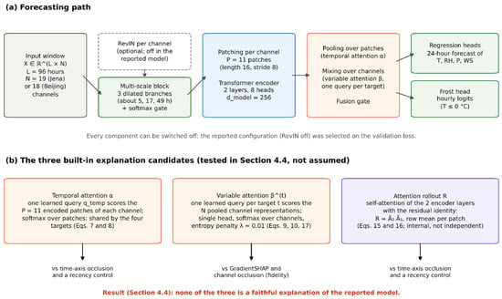
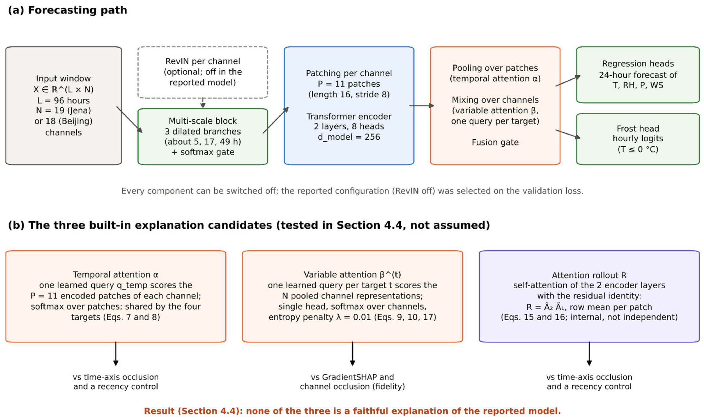
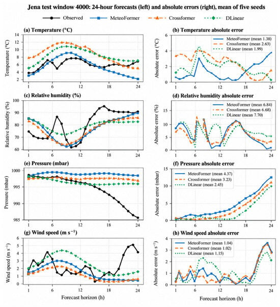
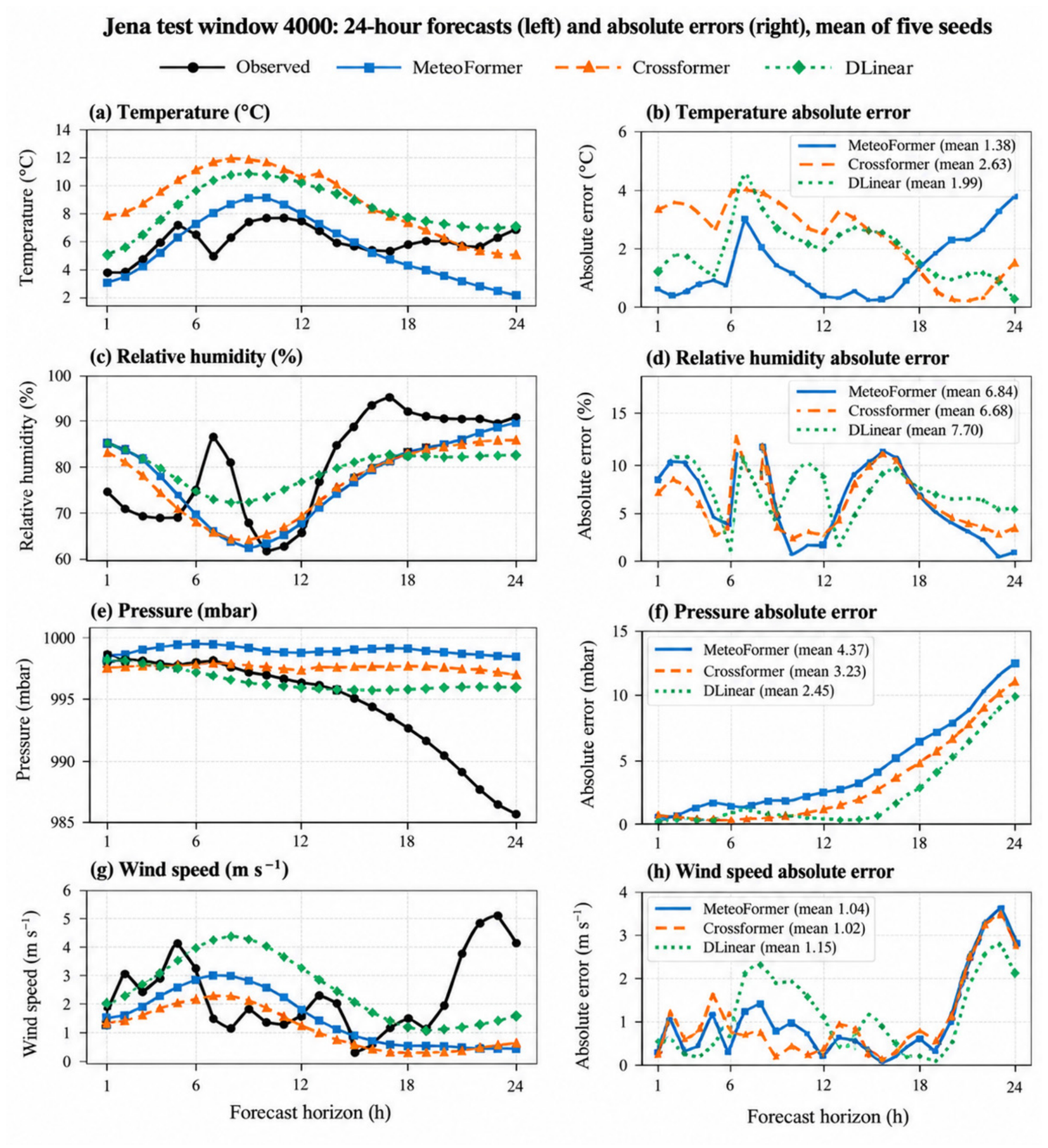
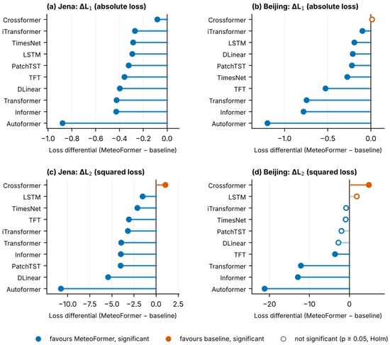
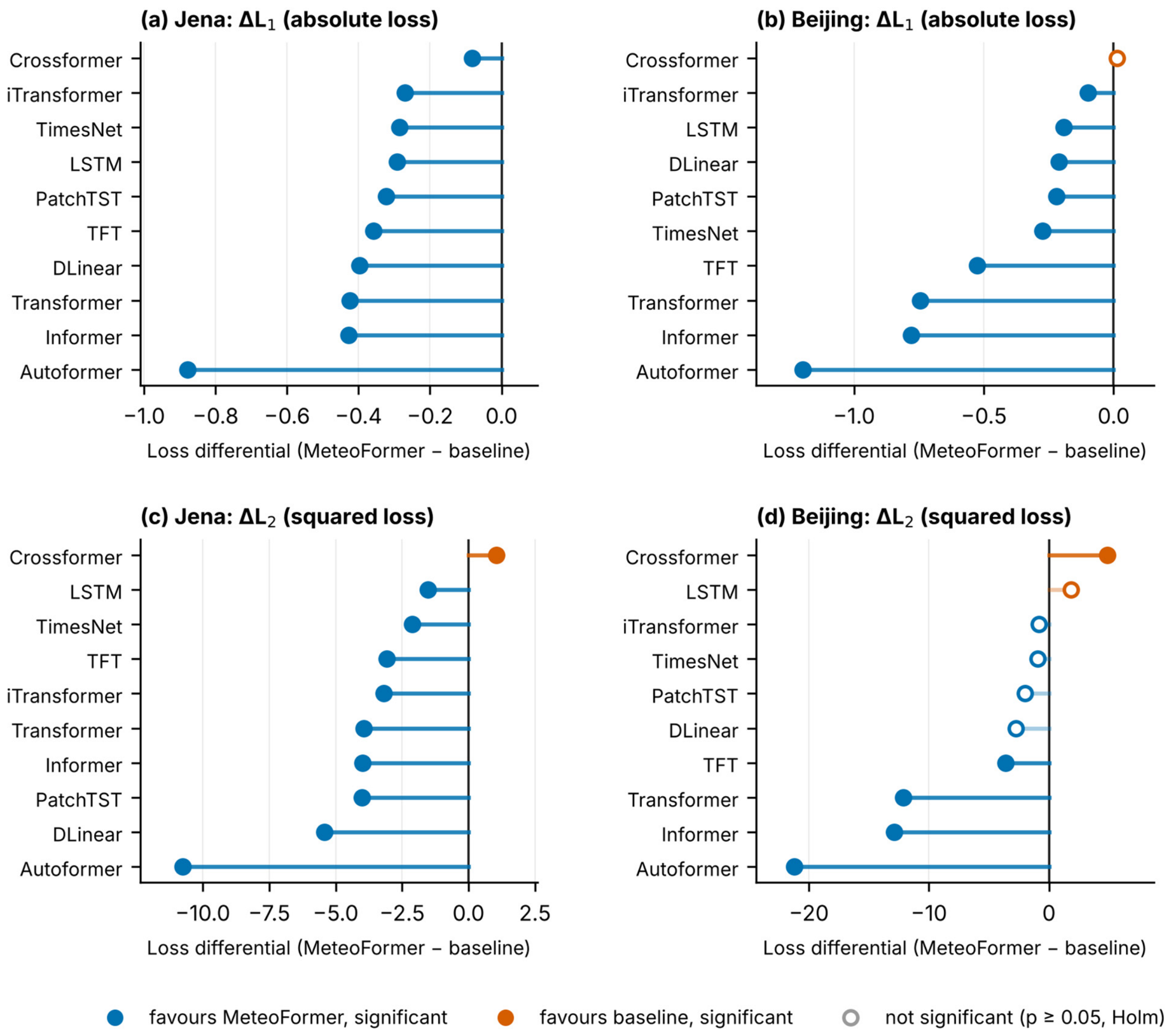
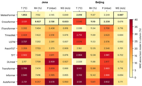
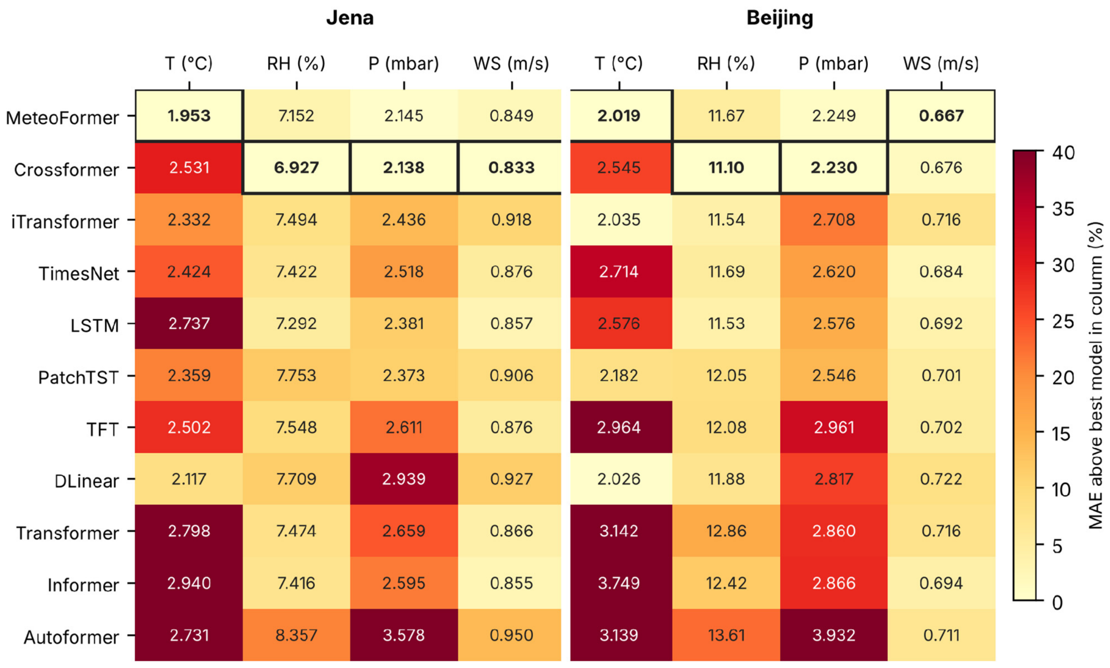
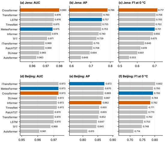
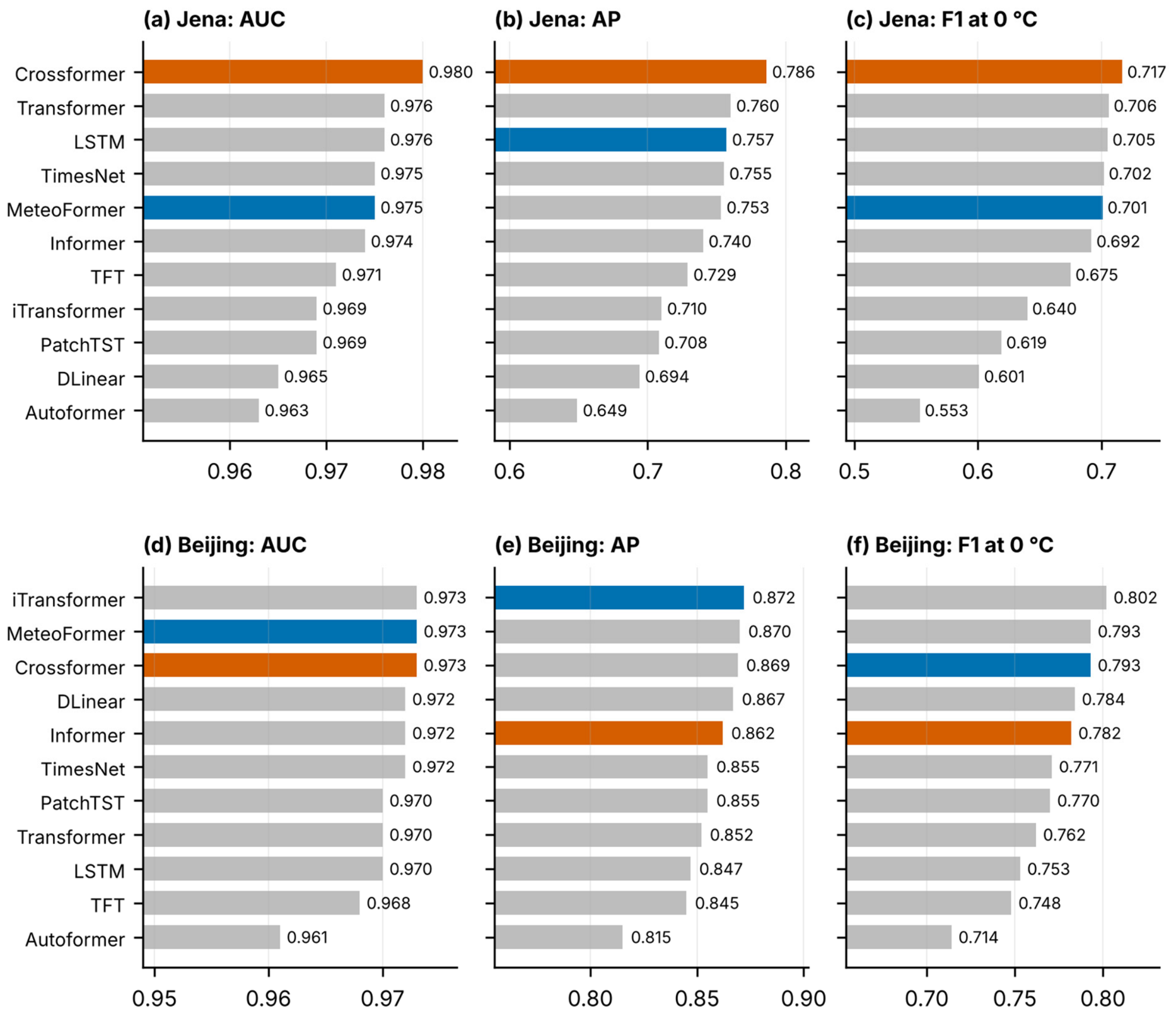
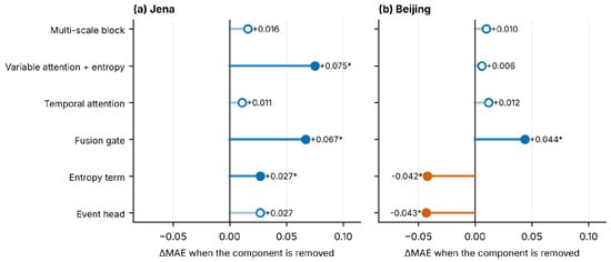
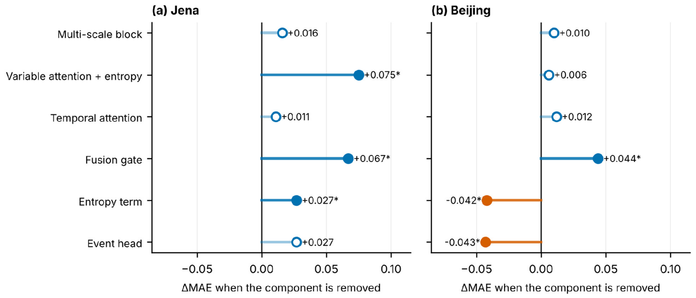
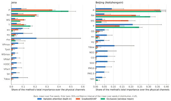
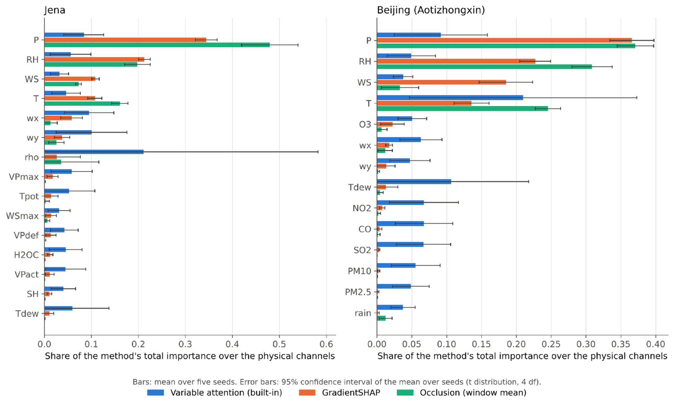
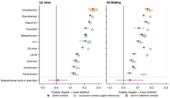
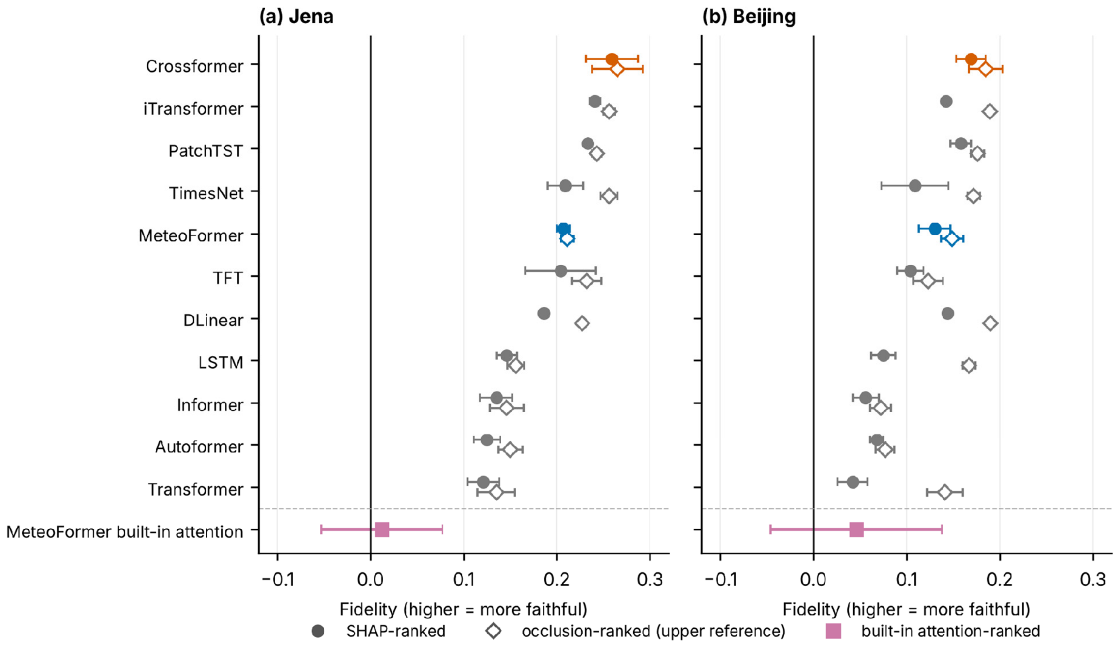
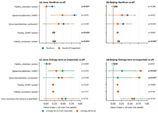
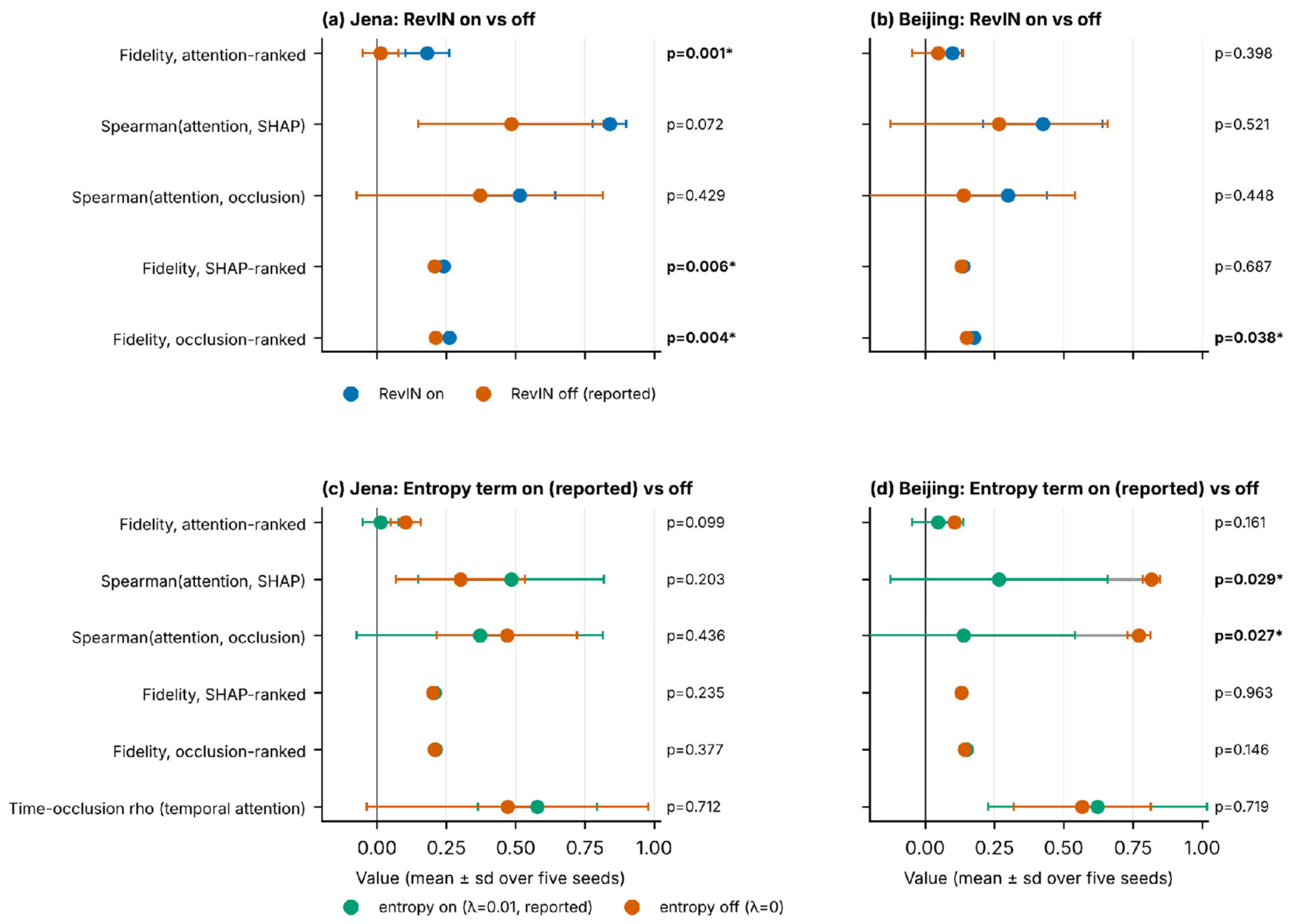
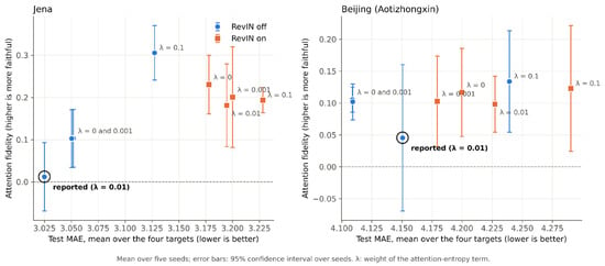
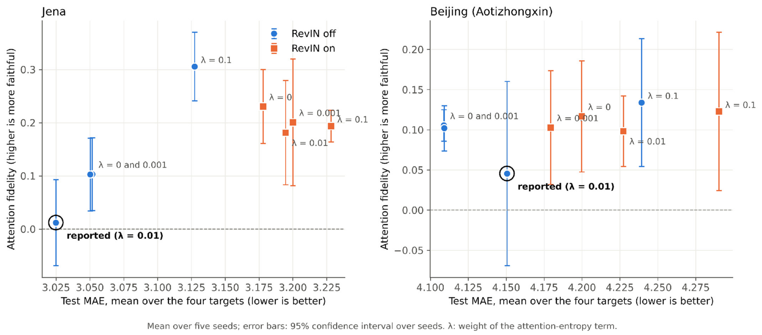
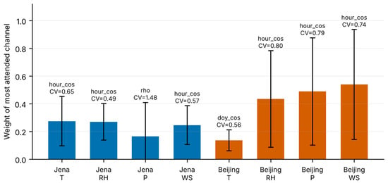
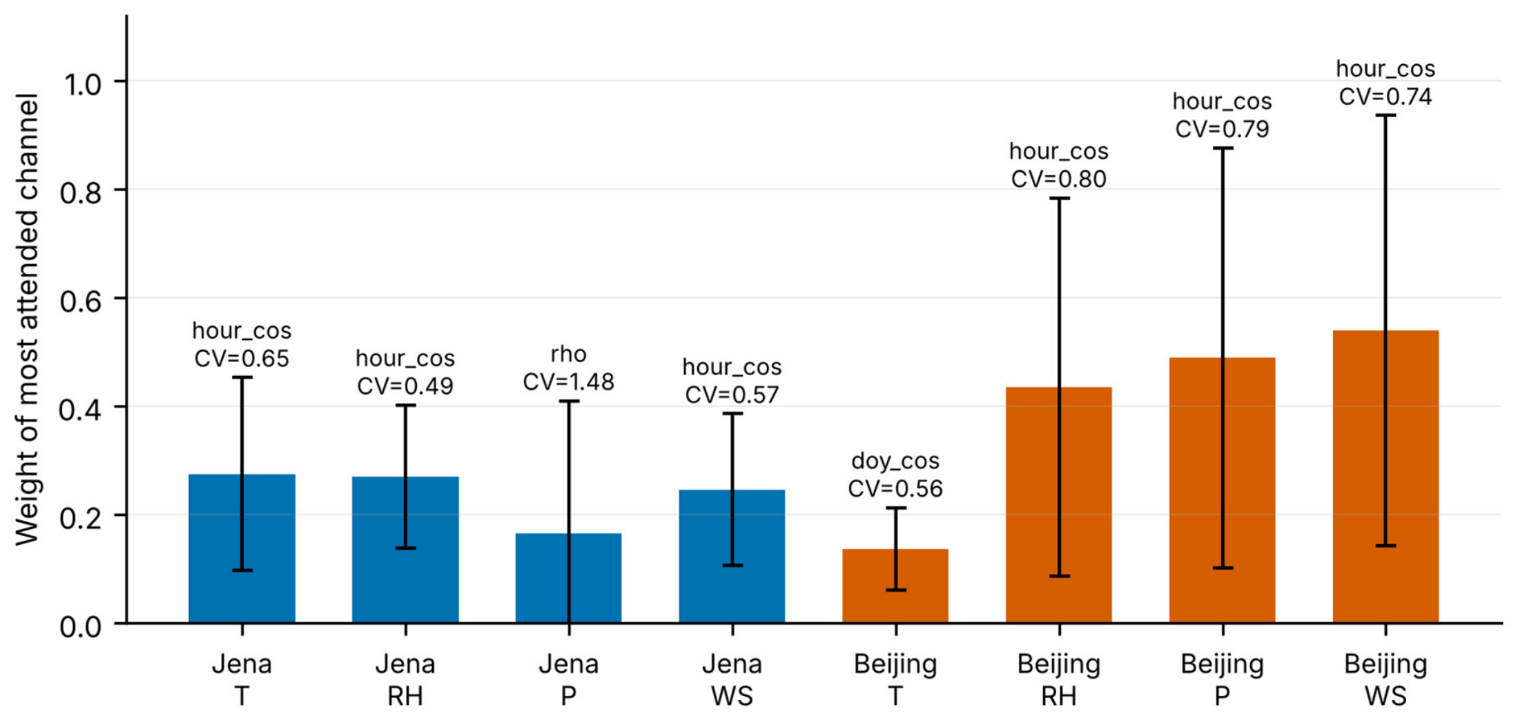
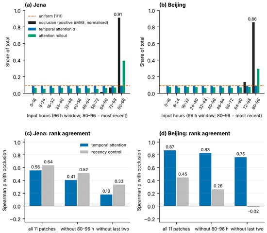
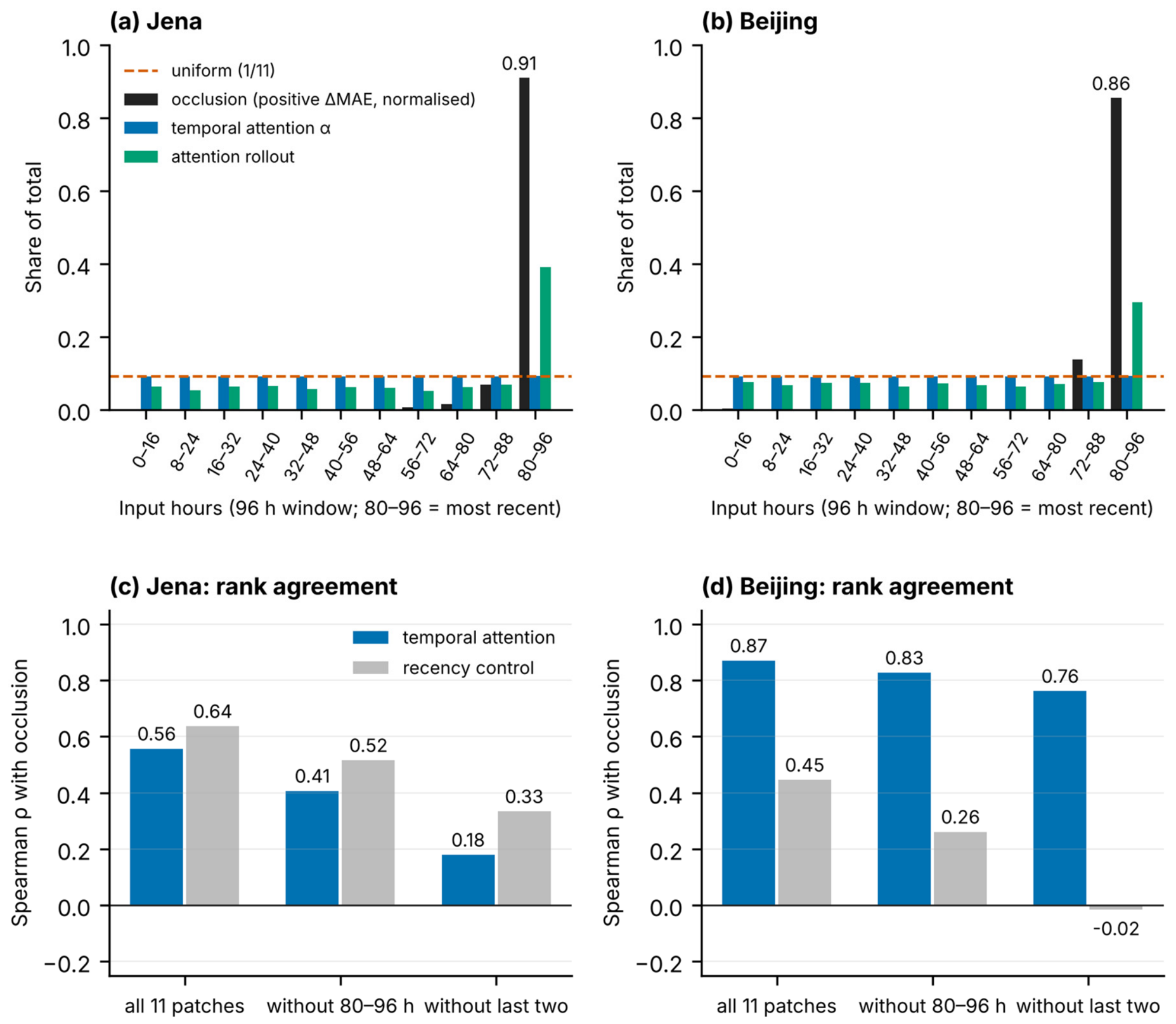
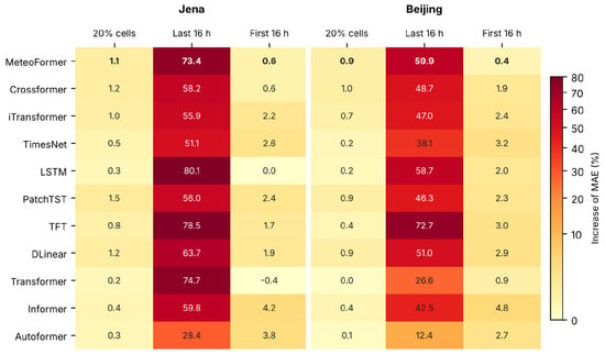
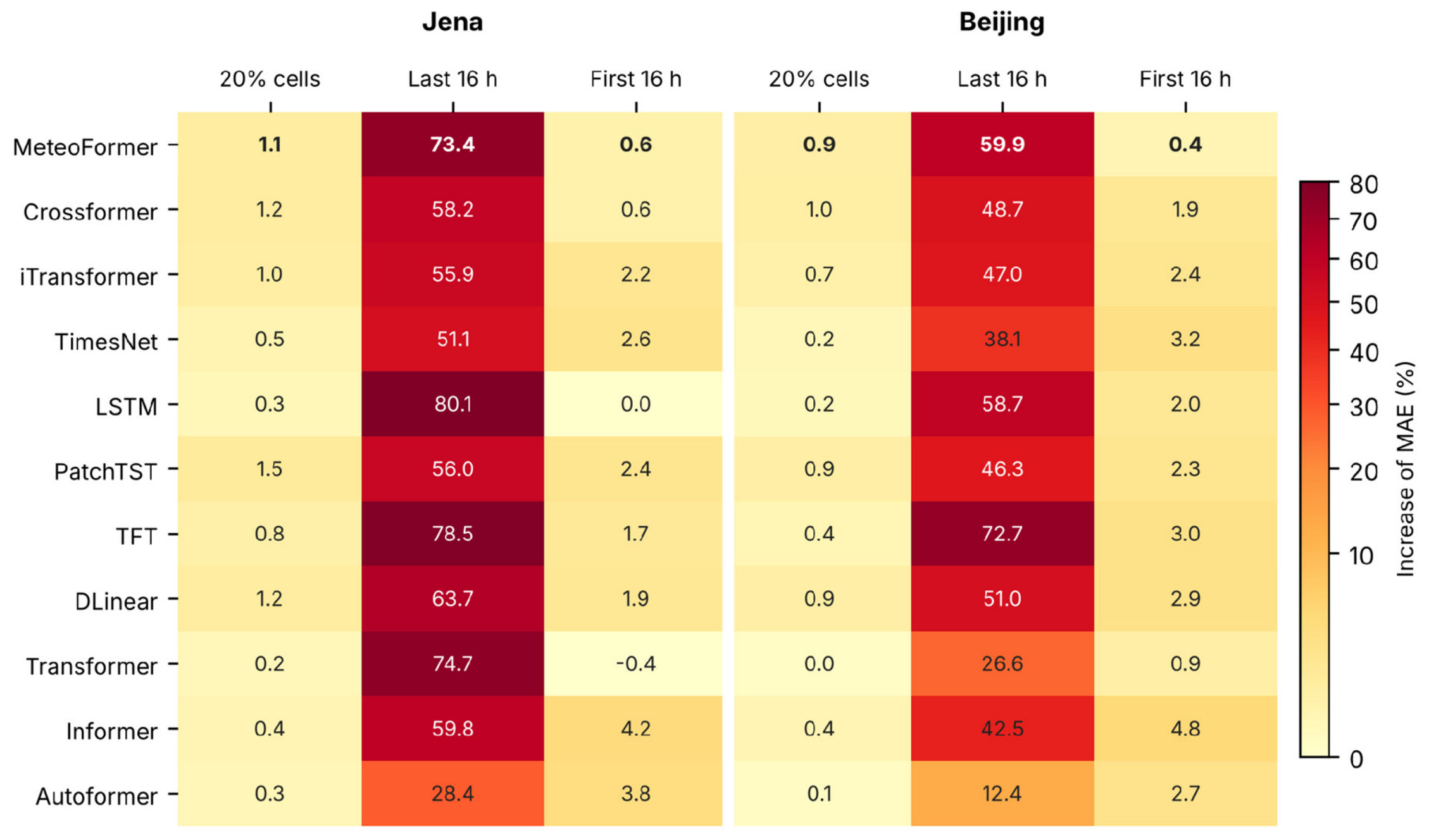
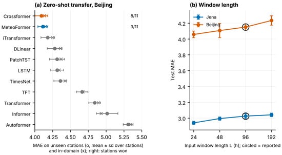
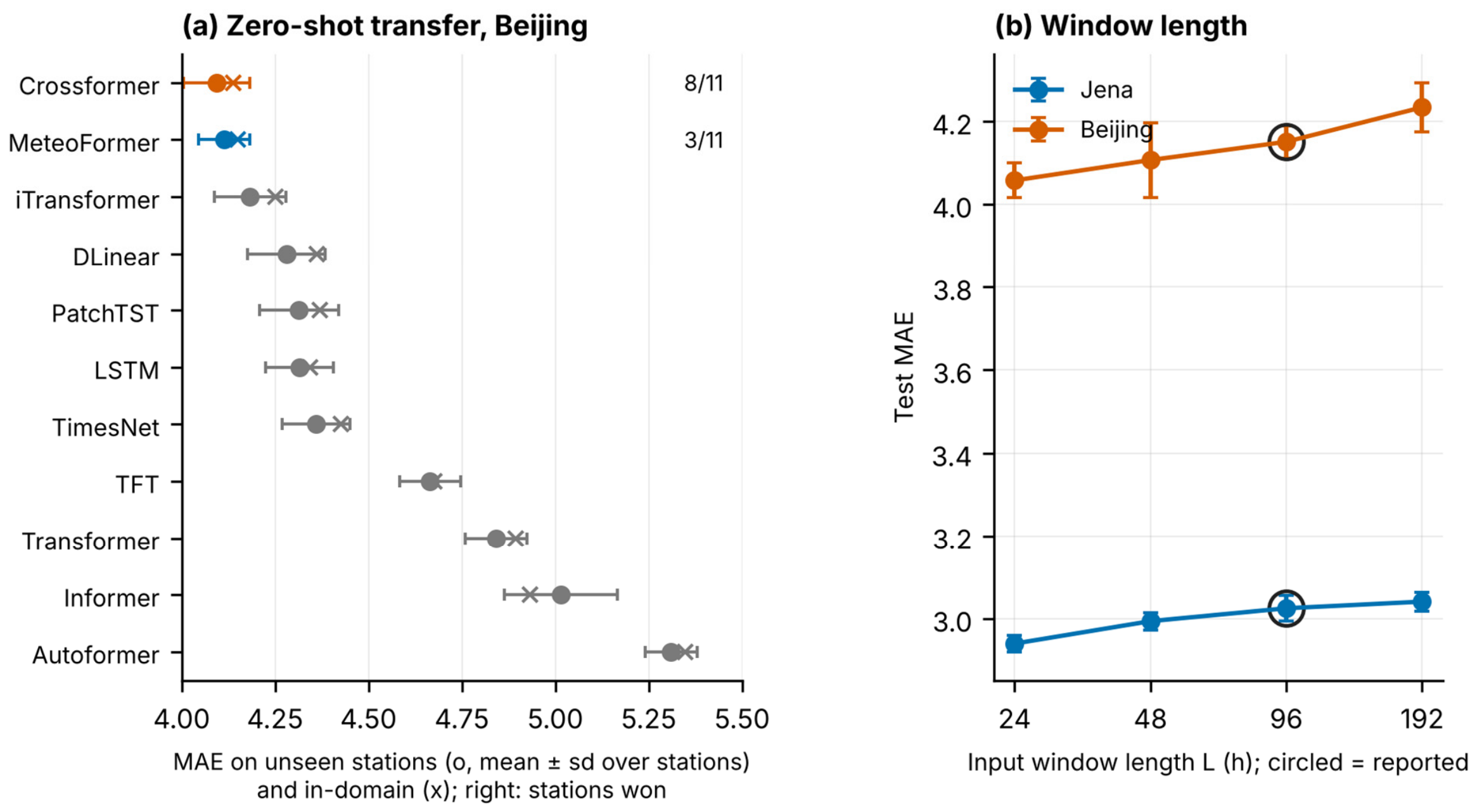

Disclaimer/Publisher’s Note: The statements, opinions and data contained in all publications are solely those of the individual author(s) and contributor(s) and not of MDPI and/or the editor(s). MDPI and/or the editor(s) disclaim responsibility for any injury to people or property resulting from any ideas, methods, instructions or products referred to in the content. |
© 2026 by the authors. Licensee MDPI, Basel, Switzerland. This article is an open access article distributed under the terms and conditions of the Creative Commons Attribution (CC BY) license.