Evaluation of WindNinja Simulations in Canyon Topography

Highlights

What are the main findings?

• WindNinja performed best when using gridded initialization from mesoscale weather model data, where it generally outperformed point initializations.
• WindNinja also performed better in moderately complex terrain rather than in very steep and deeper canyons, where the model struggled to reproduce diurnal circulations and other complex flow patterns.

What are the implications of the main findings?

• WindNinja is best used as a high-resolution terrain adjustment tool for mesoscale forecasts in moderately complex terrain—not as a replacement for WRF or observations in highly complex canyon environments.
• For best results, users should initialize WindNinja using a spatially broad, gridded dataset versus its native point initialization commonly used in the field by land managers.

Abstract

This study describes a validation of the surface wind model WindNinja conducted over different types of complex terrain. The Weather Research and Forecasting model (WRF) 2 km output was used as input for our WindNinja simulations. We tested the surface wind model for two case sites in California characterized by canyons of different terrain complexity. Simulations were conducted with different initialization methods and numerical solvers within WindNinja. The first simulations were conducted by initializing the model from a singular point. Further simulations were initialized using a spatial method with explicit input values over the whole modeling domain. The simulation results were then compared to WRF model output to see if WindNinja could improve upon the mesoscale model’s forecast in a canyon setting. Statistical error metrics were calculated to compare the model output to the observations and thus validate the performance of both WindNinja and WRF at several stations for the two case sites. WindNinja performed only marginally better than WRF over simpler terrain. WRF performed best in complex terrain with steep canyons compared to WindNinja, which struggled with increased wind speeds at peaks and ridges.

1. Introduction

Numerous wildland fires in complex terrain and canyons have produced extreme fire behavior and caused firefighter fatalities [1]. In these environments, fire spread can accelerate rapidly, and unlike typical upslope propagation, canyon fires can exhibit eruptive behavior depending on terrain characteristics, such as width and steepness [2,3].

Terrain significantly influences wind speed and direction, key drivers of fire behavior. Examples include wind channeling in valleys and acceleration over ridges [4]. Winds in mountainous regions are broadly classified as dynamically and thermally driven [5]. Dynamically driven winds are particularly relevant for extreme fire behavior due to their high surface speeds and include downslope windstorms (e.g., Santa Ana and Diablo winds) [6], mountain waves, synoptic flow channeling, and gap winds. Their behavior depends on atmospheric stability, flow velocity, and terrain characteristics [7]. Thermally driven winds, associated with diurnal cycles, can also rapidly alter fire behavior.

Accurate wind prediction over complex terrain remains challenging. Early studies focused on understanding flow over simple hills (<17° slopes) [8], including investigations of low ridges [9]. These emphasized mean velocity and turbulence intensity, with limited understanding of turbulence structure [10]. The Askervein Hill experiment later provided a key dataset for boundary layer flow over terrain [11], supporting model validation due to its relatively smooth slopes [12].

Atmospheric models are generally categorized as prognostic or diagnostic. Prognostic models, such as numerical weather prediction systems, solve conservation equations for mass, momentum, energy, and moisture [13]. While increasing computational power has enabled higher-resolution simulations, terrain-following coordinates introduce errors over steep slopes due to grid distortion [14,15,16,17]. Additionally, studies have shown that mesoscale models, such as the WRF model, show wind speed and direction errors that are linked to terrain representation [18,19,20]. Alternative modeling approaches have been developed to address these limitations [21,22,23].

WindNinja is a diagnostic model designed to simulate terrain-induced wind flow for wildland fire applications [24]. It produces microscale wind fields (typically 100–200 m resolution) without time stepping, making it computationally efficient. It can also process sequential forecast data to generate refined wind fields over time [13]. Diagnostic models like WindNinja conserve mass, momentum, and energy while adjusting an initial wind field derived from observations or weather models. Its primary solver minimizes deviations from the input field while conserving mass locally for each grid cell and globally for the entire computational domain. WindNinja does so by taking the square difference between adjusted and initial wind field values [13]. A more advanced WindNinja solver incorporates both mass and momentum conservation using OpenFOAM [25], solving steady-state, incompressible RANS equations under neutral stratification.

Previous validation studies show that WindNinja’s mass-conserving solver captures terrain-modified flow near the surface but struggles in regions dominated by momentum effects, such as lee-side recirculation zones [13,24,26]. To address this, the momentum-conserving solver was introduced to improve simulations without substantially increasing computational cost.

Downscaling weather model output using WindNinja is one method to better resolve surface winds in complex terrain. However, prior evaluations have often focused on simpler terrain [27]. In more complex environments, such as Big Southern Butte, WindNinja improved wind predictions compared to mesoscale models, particularly during high-wind events, but it failed to capture microscale processes like lee-side recirculation due to the lack of momentum conservation [28].

Past research has compared WindNinja’s performance over simpler and more complex topography [28]. The study presented in this paper provides a new validation of WindNinja over highly complex terrain, specifically in canyons. Simulations were initialized using large-scale weather model data and downscaled to produce higher-resolution wind fields. Different initialization methods and numerical solvers were evaluated, including a point-based approach commonly used in practice and a spatial method using gridded data. WindNinja results were compared with mesoscale model output to assess its ability to improve wind predictions for two specific canyon environments.

2. Methods

2.1. Model Background

WindNinja is a diagnostic wind model developed in 2005 by the US Forest Service Missoula Fire Sciences Laboratory [13]. As mentioned previously, WindNinja could only provide mass-conserving simulations to its users in its native form. Over the years, the model has gone through continuous development, such as the implementation of a computational fluid dynamics (CFD) solver [28]. The model version used for this study was WindNinja 3.9.0.

In this research, WindNinja simulations were conducted over complex terrain for two different case sites. For each of these sites, several simulations with different setups were performed. The first simulations were done using the point initialization method, and further simulations were performed with the gridded initialization method of WindNinja. Most of the case studies were done using WindNinja’s conservation of mass solver. Simulations using the conservation of mass and momentum solver were done solely for one of the gridded initialization case sites.

2.2. WindNinja Framework

Both of the WindNinja solvers solve for neutrally stratified flow. The model does, however, include thermal parameterizations to account for thermal effects, such as diurnal slope winds. Heating or cooling of the air close to the slope leads to upward or downward flow, which we know as diurnal slope winds [7,29]. The orientation of the slope toward the sun affects the slope’s heating, which has a direct effect on the intensity of the upslope winds. Other factors also affect the strength of the diurnal winds. These would be surface properties, which affect how well the solar energy is absorbed by the surface, but also factors like slope steepness and cloud cover can be taken into consideration. WindNinja has a built-in diurnal slope flow model, which accounts for sensible surface heat flux, distance to valley bottom or ridge crest, and slope angle.

WindNinja’s slope flow model is the same as Mahrt [30] for shooting flow. The model is one-dimensional and uses a buoyancy-steered flow over a slope. With this model, the strength of the slope flow is measured as a function of acceleration distance, percent slope, surface and entrainment drag parameters, and surface sensible heat flux. Before considering the slope component, WindNinja starts its simulations by initializing the flow domain with specified wind speed and direction input, and the equation:

$$U(z)=U(z_1){\displaystyle \frac{ln\left(\frac{z}{z_0}\right)-{\Psi }_m\left(\frac{z}{L}\right)}{ln\left(\frac{z_1}{z_0}\right)-{\Psi }_m\left(\frac{z_1}{L}\right)}}$$

(1)

where $U$ is the wind speed, $U\left(z_1\right)$ is the wind speed at the measurement height $z_1$, L is the Monin–Obukov length, and ${\Psi }_m$ is a stability correction function. After these prior steps, WindNinja lastly runs its numerical solver, which is either solely mass-conserving or both mass- and momentum-conserving [27,28,31].

2.3. WRF Simulation Background

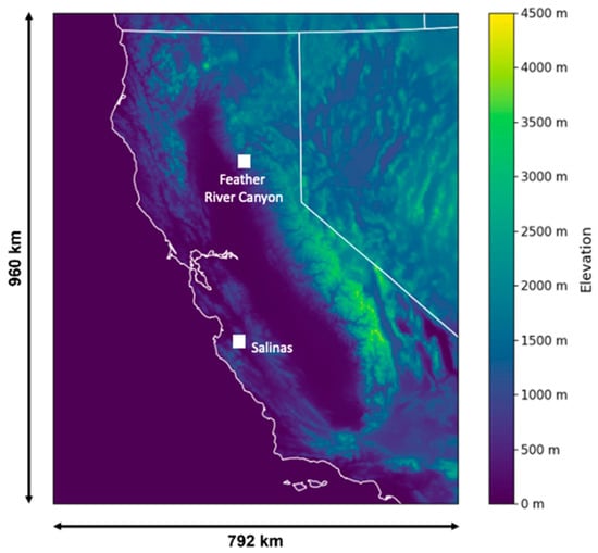
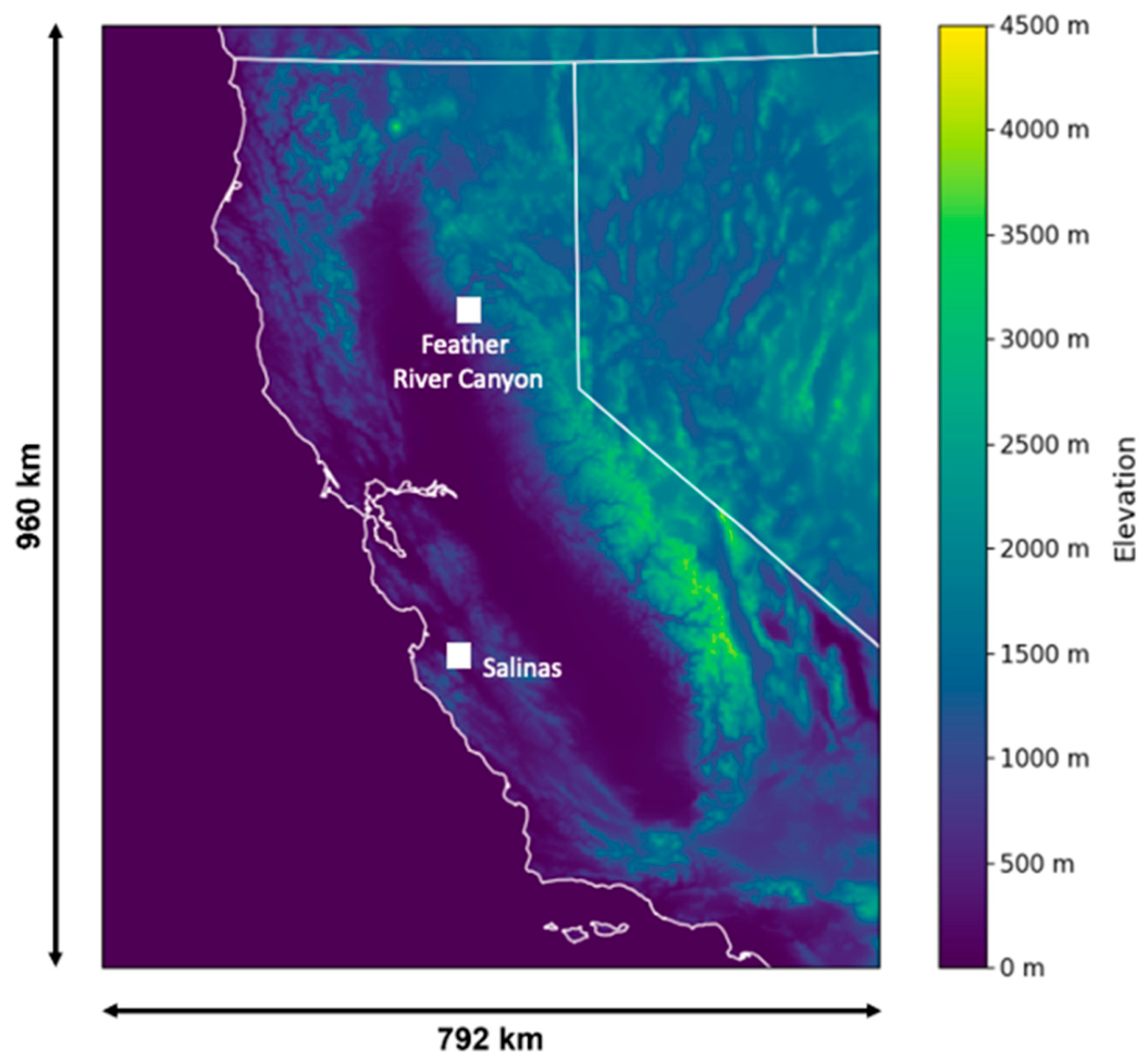
The WRF data used to initialize the WindNinja simulations are from WRF simulations using version 4.1.2, as discussed in [32]. The output from domain 3 was used for the analysis, which has a horizontal grid spacing of 2 km. The model’s west–east grid dimensions are 397, and the south–north dimensions are 481. With this, a total modeling domain of 792 km wide (x-axis) and 960 km long (y-axis) is available (Figure 1).

Figure 1. WRF domain 3 covers Central and Northern California, and each site for analysis is indicated as white squares: Salinas and Feather River Canyon. The white outline symbolizes the California state boundary.

The WRF simulations were initialized and forced using NCEP Climate Forecast System Reanalysis Version 2 (CFSRv2) data. The model simulation produced hourly meteorological fields to capture diurnal variations in wind speed and boundary layer dynamics. The time-varying sea surface temperature (SST), sea ice, vegetation fraction, and albedo were updated along with deep soil temperature and skin SST. Physics parameterizations are summarized in Table 1 and include the Noah-MP land surface model, MYNN surface-layer and third-order planetary boundary layer (PBL) schemes, Thompson microphysics, and RRTMG longwave and shortwave radiation. The Kain–Fritsch cumulus parameterization was applied only on the outer domain. Topographic shading and slope-dependent radiation effects were included to improve surface energy balance calculations, particularly for complex terrain [32].

Table 1. WRF physics parameterizations used in this study.

Physics Component	WRF Configuration
Land surface model	Noah-MP
Surface layer	MYNN
Planetary boundary layer	MYNN third-order
Microphysics	Thompson
Longwave and shortwave radiation	RRTMG
Cumulus parameterization	Kain–Fritsch on 18 km outer domain only
Terrain radiation effects	Topographic shading and slope-dependent radiation on the 2 km inner domain

2.4. WindNinja Simulation Setup

Simulations were conducted for two different sites in Northern California (Figure 1): a steep and narrow canyon located near Salinas and the large, deep complex canyon of the Feather River Canyon. The Salinas Canyon was chosen because a field experiment was conducted there during the fall of 2022, and the days selected for the Feather River Canyon were based on days that represented typical summer fire weather patterns in the region.

2.4.1. Point Initializations

In the first set of simulations, point initialization simulations were performed, where the simulations were initialized with 2 km WRF forecast data for a specific point on the domains. To gather surface information for the simulation domain, WindNinja uses an elevation file. For the point-initialized simulations, the elevation file was first fetched with WindNinja’s built-in function for both case sites. The built-in function allows the user to grab a USGS elevation file with a resolution of 232 m. After determining that this resolution was too coarse to resolve the canyon’s topography at the first site, the decision was made to use the higher-resolution Landscape (LCP) file for this first point-initialized case as well, and not just for the gridded initialization case as originally intended. Further information on the Landscape files is described below.

After acquiring the elevation data, WindNinja requires further surface information. The model accounts for the drag that vegetation exerts on the wind flow. If the elevation file in use does not provide information on canopy and fuel parameters, WindNinja allows the user to choose a dominant vegetation type of grass, brush, or trees, which corresponds to a roughness height of either 0.01, 0.43, or 1.0 m, respectively [23,29,33]. For the mesh resolution of the simulations, the finest possible setting that WindNinja suggested for the respective domain was chosen. Lastly, WindNinja’s diurnal slope flow model setting was also enabled for the point initialization simulations (Table 2).

Table 2. WindNinja point initialization simulation settings for both case sites.

Site	Solver	Surface Input—Vegetation	Surface Input—Mesh Resolution	Diurnal Input	Wind Input	Output
Salinas	COM	From LCP	Fine—110 m	Diurnal winds enabled	Point Initialization	Height: 10 m Output Speed Units: m s−1
Feather River Canyon	COM	Trees	Fine—327 m	Diurnal winds enabled	Point Initialization	Height: 10 m Output Speed Units: m s−1

The wind output for these point initialization simulations is stored in cells with a specific number, each of which has a simulated wind speed value (m s⁻¹) and wind direction value (degrees), as well as latitude and longitude coordinates. Given the coordinates of a specific station, we examine the four cells closest to the given station and extract their wind data. For each timestep, the wind data of those four cells is then averaged to determine a singular wind speed and wind direction value as the respective simulation result for each station. To account for wind direction being a circular variable, the Jammalamadaka and Lund [34] process was followed, where the mean wind direction is found by first calculating the summations of the sines and cosines of the wind directions. These summations were then used to calculate an average wind direction based on quadrant-specific conditions.

2.4.2. Gridded Initialization

The gridded initialization simulations were conducted with WindNinja’s command line interface (CLI), and the simulation settings were listed in a configuration file. Running simulations in WindNinja’s CLI allows for a more customizable simulation setup and offers more features, which are not represented in WindNinja’s GUI, such as the “griddedInitialization” method. Same as with the previous initialization method, 2 km WRF forecast data was used as input. However, in this case, the simulations are not just initialized with forecast data for one point but use a spatial method to initialize the model with explicit data values over an entire grid. As used for point initializations, LCP files were used as elevation files. Vegetation parameters obtained from LANDFIRE 2022 were Vegetation Cover, Height, and Type. The projection of the LANDFIRE data is NAD 1983. The conservation of mass solver was also used on all gridded simulation cases, and the diurnal winds option was also enabled. WindNinja’s more advanced conservation of mass and momentum solver was also used for some of the simulations. This way, the performance of both solvers could be tested and compared to each other (Table 2 and Table 3).

Table 3. WindNinja gridded initialization simulation settings as found in the configuration file for the Salinas site. This example is for simulations using the conservation of mass solver. When running the conservation of mass and momentum solver, the bottom two lines must be added.

Configuration Parameter	Value/Setting
uni_air_temp	15
num_threads	1
input_speed_units	mps
output_wind_height	10
initialization_method	griddedInitialization
input_wind_height	10
output_speed_units	mps
units_input_wind_height	m
units_output_wind_height	m
time_zone	UTC
mesh_resolution	250
units_mesh_resolution	m
ascii_out_resolution	250
units_ascii_out_resolution	m
write_ascii_output	true
uni_cloud_cover	0
cloud_cover_units	percent
air_temp_units	C
diurnal_winds	true
year	2022
month	10
day	21
hour	00
minute	00
input_speed_grid	wdsp_example.tif
input_dir_grid	wddr_example.tif
output_path	/home/015966717/Gridded_Output_Salinas
elevation_file	/home/015966717/Gridded_Input_Salinas/Salinas.lcp
momentum_flag	true
number_of_iterations	200

For these gridded simulations, WindNinja uses 2 km WRF data as wind input and downscales it to a higher resolution of 250 m. The downscaling is done with the help of the high-resolution topography data from the LCP file, which has a resolution of 30 m. Since the LCP file’s projection is in NAD83, the WRF data needs to be reprojected into the same projection. A common issue is missing data values around the border of an elevation file due to warping. To avoid missing data values, the LCP file was cropped while also making sure that the data extent of the WRF GeoTIFF files is larger than that of the LCP file.

2.5. Data and Statistical Comparisons

For each WindNinja simulation, the 6Z WRF forecast data of each simulated day was used to have better alignment with observation periods and operational relevance. The data used were the 10 m surface wind data. The observational data used for the validation of WindNinja’s performance were taken mostly from surface weather stations, and the data were downloaded through MesoWest [35]. All surface weather station metadata are provided in Table 4.

Table 4. Metadata of the observational stations used for the evaluation.

Site	Station	Coordinates	Elevation (m)	Site Descp.
Salinas	385PG	36.66739, −121.5205	406	Ridge
	Bottom RAWS	36.660694, −121.528867	138	Canyon
	Ridge RAWS	36.664217, −121.519633	400	Ridge
Feather	275PG	39.90248, −121.24978	1750	Ridge
	335PG	40.03870, −121.13126	1036	Canyon
	404PG	39.96012, −121.28009	623	Valley
	PG129	40.03713, −121.18715	1930	Peak
	PG292	40.02061, −121.06455	849	Valley
	PG326	39.82908, −121.47164	1299	Ridge
	PG458	39.86850, −121.17419	1576	Valley
	PG746	40.06602, −121.11797	1932	Peak

For the Salinas case, the data for two of the three stations were taken from remote automatic weather stations (RAWS) that had been installed on site for a field experiment and additional data for model comparisons. Those two RAWS were recording data at a height of 2 m AGL (above ground level). On the other hand, standard weather stations in the utility network measure at a height of 6.1 m AGL. Since the WRF data output is at 10 m AGL, but the observations are at different heights, the WindNinja wind speed output was interpolated to the specific height at which the observations were taken. By applying the following equation from Sedefian [36], the simulation wind speeds were corrected as such:

$$S_{corr}= {\displaystyle \frac{(S \ast ln \left(\frac{O_h}{z_0}\right) )}{ln \left(\frac{S_h}{z_0}\right) }}$$

(2)

$S_{corr}$ is the corrected simulation wind speed, $S$ is the simulation wind speed, $O_h$ is the observational wind speed height, $S_h$ is the simulation wind speed height, and $z_0$ is the roughness length. The roughness length values were taken from Hahmann et al. [37], who based their values on the USGS land use categorization. For the Salinas case, a roughness length $z_0$ of 0.12 m was chosen, which is classified as the shrubland land cover class. For the Feather River Canyon case, $z_0$ of 0.9 m was defined, which classifies as needleleaf forest. For both case sites, the roughness length value for the predominant shrubland class across the modeling domain was selected. This approximate approach was chosen for simplicity reasons.

The WRF data have a temporal resolution of 1 h, and thus the WindNinja output is also hourly. The observational data have higher temporal resolutions of 5 min for the AWS setup at the Salinas site and 10 min for the utility surface stations. Since this is the case, the observations needed to be averaged for each hour to match the temporal resolution of the model data for the comparison.

To compare WindNinja’s performance to the large-scale weather model WRF, the 6Z forecast of each of the simulated days was extracted for the specific locations of the stations. This was done by fetching the wind data from the nearest of the four grid points surrounding the coordinates of the chosen station. The WRF data were also height-corrected with Equation (4) that was also used to interpolate the WindNinja output.

In this study, two statistical error metrics were calculated to validate the WindNinja simulations and WRF output. The statistical metrics used were correlation coefficient (r) and mean absolute error (MAE). For the correlation coefficient, the Pearson correlation coefficient was calculated, which computes the linear relationship between two variables. Both r and MAE were calculated for all hours of the simulated days. Analyses also focused on morning hours from 0500 to 1100 LT to capture the morning transition period, and afternoon hours from 1200 to 1800 LT. In the case of the wind speed statistics, standard approaches could be used, which means that, in the case of r, the Pearson correlation coefficient was calculated as such:

$$r={\displaystyle \frac{{\Sigma }_{i=1}^N\left(S_i-\underset{\_}{S}\right)\left(O_i-\underset{\_}{O}\right)}{\sqrt{{{\Sigma }_{i=1}^N\left(S_i-\underset{\_}{S}\right)}^2 {{\Sigma }_{i=1}^N\left(O_i-\underset{\_}{O}\right)}^2}}}$$

(3)

where N is the total number of simulation time steps, $S_i$ is the model wind speed, and $O_i$ stands for the observational wind speed, $\underset{\_}{S}$ is the mean simulation wind speed, and $\underset{\_}{O}$ is the mean observational wind speed [15].

The MAE statistics of wind speed are in m s⁻¹ and were calculated as such:

$$MAE={\displaystyle \frac{1}{N}}\sum _{i=1}^N\left|S_i-O_i\right|$$

(4)

In the case of wind direction, circular statistics based on Jammalamadaka and Lund [34] were followed, since wind direction is a circular variable. The statistics for wind direction are calculated from the differences between sines and cosines of the simulations and observations. When calculating the correlation coefficient for wind direction in Equation (5), we see that it looks very similar to Equation (3). However, in the case of circular statistics, we work with the sines of $S_i$, $O_i$, $\underset{\_}{S}$, and $\underset{\_}{O}$, which are wind directions:

$$r_c={\displaystyle \frac{{\Sigma }_{i=1}^{N}sin\left(S_i-\underset{\_}{S}\right)sin\left(O_i-\underset{\_}{O}\right)}{\sqrt{{\Sigma }_{i=1}^N{sin}^2\left(S_i-\underset{\_}{S}\right){ \Sigma }_{i=1}^N{sin}^2\left(O_i-\underset{\_}{O}\right)}}}$$

(5)

MAE for circular statistics is in degrees and was calculated following Kochanski et al. [38]:

$${MAE}_c={\displaystyle \frac{180}{\pi }}{\displaystyle \frac{1}{N}}\sum _{i=1}^N\left|sin(S_i-O_i)\right|$$

(6)

2.6. Case Sites

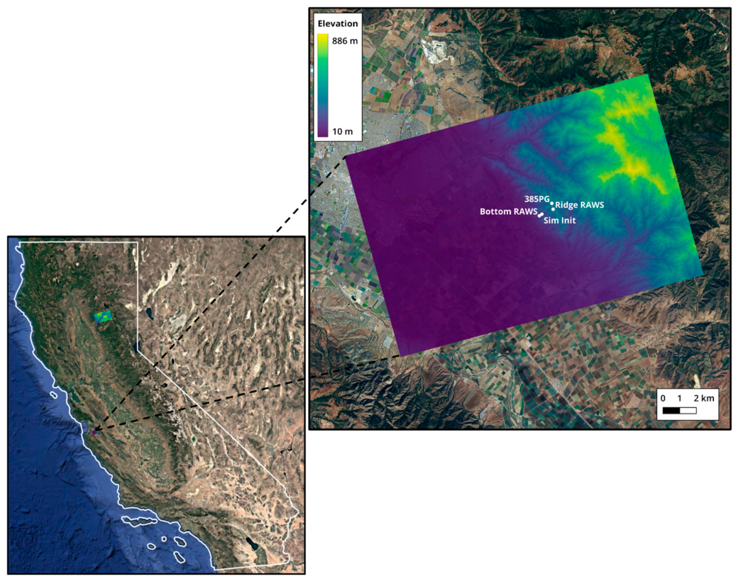
The first case site chosen for the WindNinja simulations is located in the Gabilan Range east of Salinas, CA (Figure 1 and Figure 2) because it was an area where additional weather stations were installed for collecting observations. Salinas is located on the Central Coast of California and is less than 16 km from the Pacific Ocean. The climate is thus strongly influenced by the ocean through on- and offshore winds and the presence of the marine layer. For the Salinas case, four days were simulated individually between 21 and 24 October 2022.

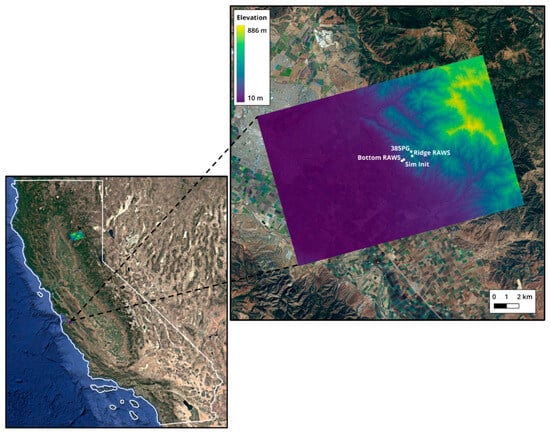
Figure 2. Map of the Salinas case site with the LCP elevation band depicted on the right. The simulation domain has an area of ca. 235 km². The 3 stations used in the analysis are displayed on the map, as well as the simulation initialization point (Sim Init) for the point-initialized simulations.

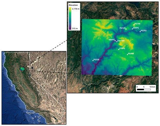
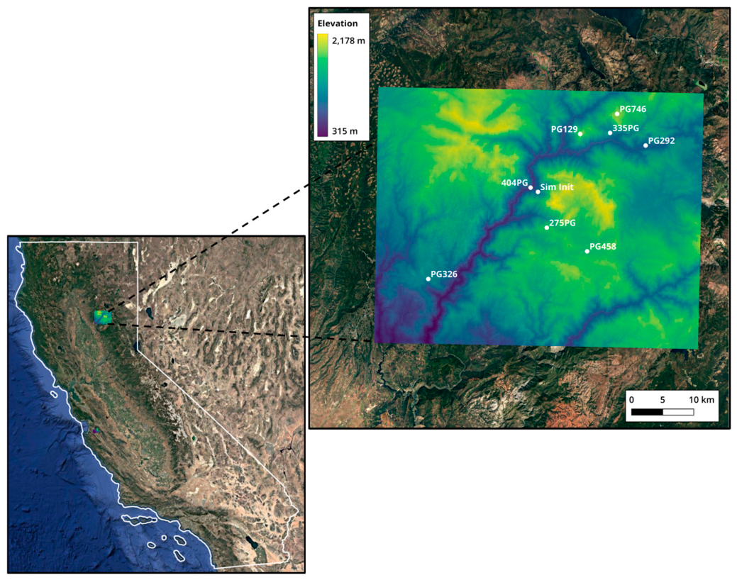
The second case site consists of larger domains located in northern California in the Plumas National Forest northeast of the town of Paradise. The domain is centered around the Feather River Canyon and stretches to Quincy in the west. The area surrounding the Feather River Canyon was selected as the second site for these simulations because of the complex topography of this canyon, which makes it difficult to simulate atmospheric flow, and also due to the region’s fire history. Several large wildfires have ravaged this area, the most devastating being the Dixie Fire in 2021 and the Camp Fire in 2018 [39]. Same as for the Salinas case, we simulated four days individually with different initialization methods. For this case, we selected four sequential summer days, which were from 17 to 20 July 2023, representing typical summer fire weather conditions.

As mentioned above, the elevation file used for the second point-initialized simulation case is from the USGS and has a coarser resolution than the LCP files. Due to the larger domain size in Figure 3, the mesh resolution was set lower at ca. 327 m, in comparison to the higher mesh resolution of 110 m of the Salinas case (Table 2). Also, since the domain is located in the Plumas National Forest area, the dominant vegetation type selected in the simulation setup in Table 2 was ‘Trees’.

Figure 3. Map of the Feather River Canyon case site with the USGS elevation file depicted on the right. The point initialization simulation domain has an area of ca. 2121 km². The 8 stations used in the analysis, along with the simulation initialization point (Sim Init), are displayed on the map.

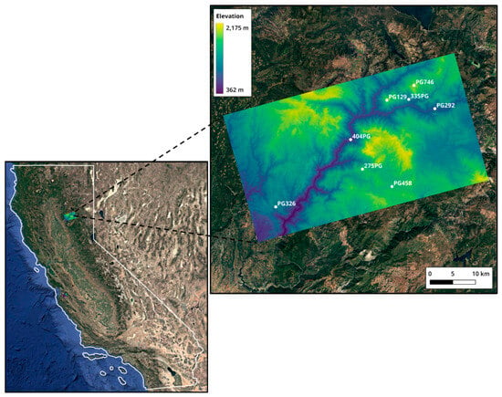
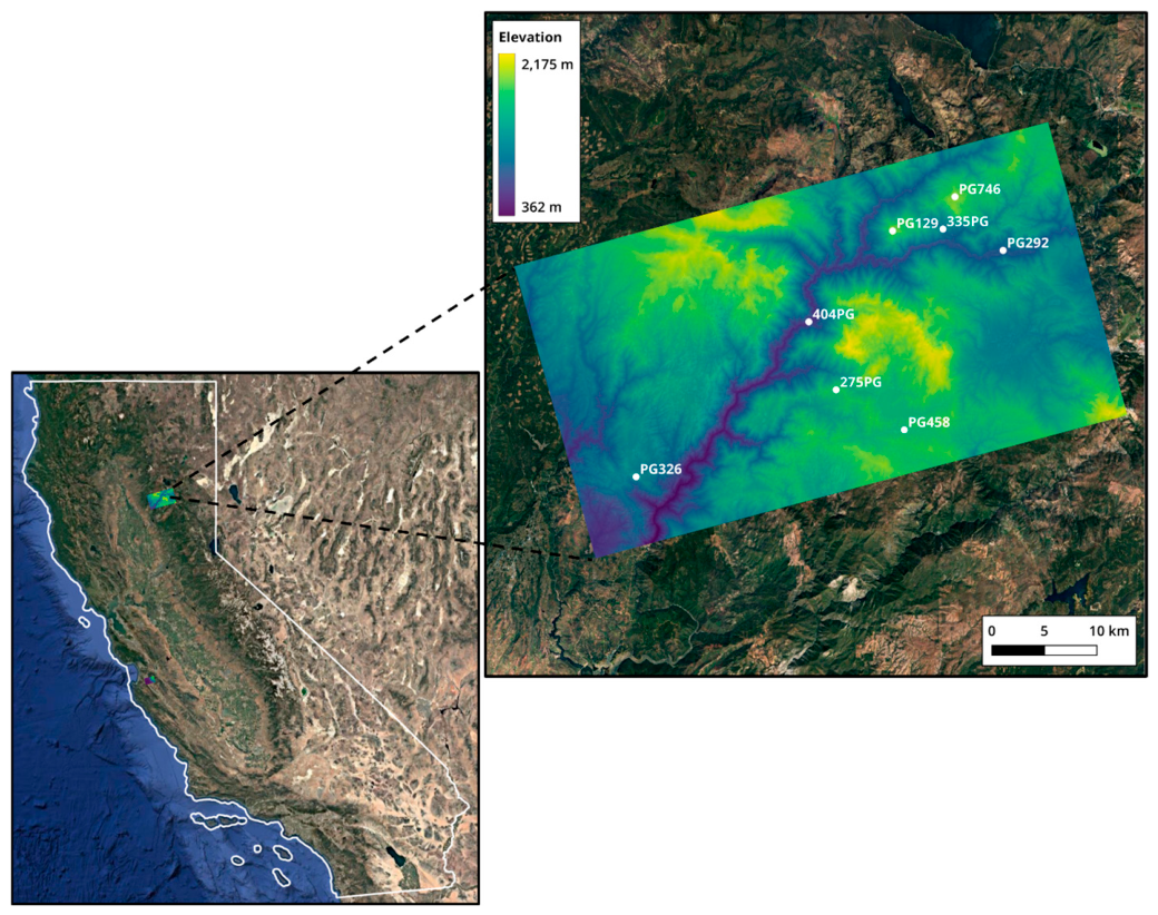
Comparing the domain of the gridded initialization simulations for the Feather River Canyon in Figure 4, we see that it is smaller than the domain of the respective point initialization simulations in Figure 3. However, the domain is still vast, with a size of ca. 1492 km².

Figure 4. Map of the Feather River Canyon case site with the LCP elevation band depicted on the right. The gridded initialization simulation domain has an area of ca. 1492 km². The 8 stations used in the analysis are displayed on the map.

To quantitatively characterize the terrain surrounding the observational sites, terrain descriptors were calculated from the 2 km WRF terrain field within a 20 km radius of each station and summarized for each study region (Table 5). The stations in Feather River Canyon were surrounded by substantially more complex terrain than those at Salinas, with a mean terrain slope of 4.33° compared with 2.71°, a local relief of 1281 m compared with 887 m, and a terrain ruggedness index (TRI) of 435 m compared with 255 m. Elevation variability was also somewhat greater in Feather River Canyon, with an elevation standard deviation of 283 m compared with 255 m at Salinas. These metrics provide a quantitative basis for characterizing the terrain surrounding the Feather River Canyon observational network as steeper and more rugged than that surrounding the Salinas stations.

Table 5. Terrain characteristics surrounding the observational stations at the Salinas and Feather River Canyon study sites. Metrics were calculated from the 2 km WRF terrain field within a 20 km radius of each station and then averaged across stations within each study region.

Site	Elevation Standard Deviation (m)	Local Relief (m)	Mean Slope (°)	Max Slope (°)	Terrain Ruggedness Index
Salinas	255	887	2.71	11.22	255
Feather	283	1281	4.33	13.99	435

3. Results

3.1. WindNinja Point Initialization

3.1.1. Wind Speed

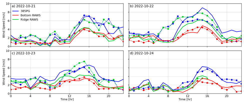
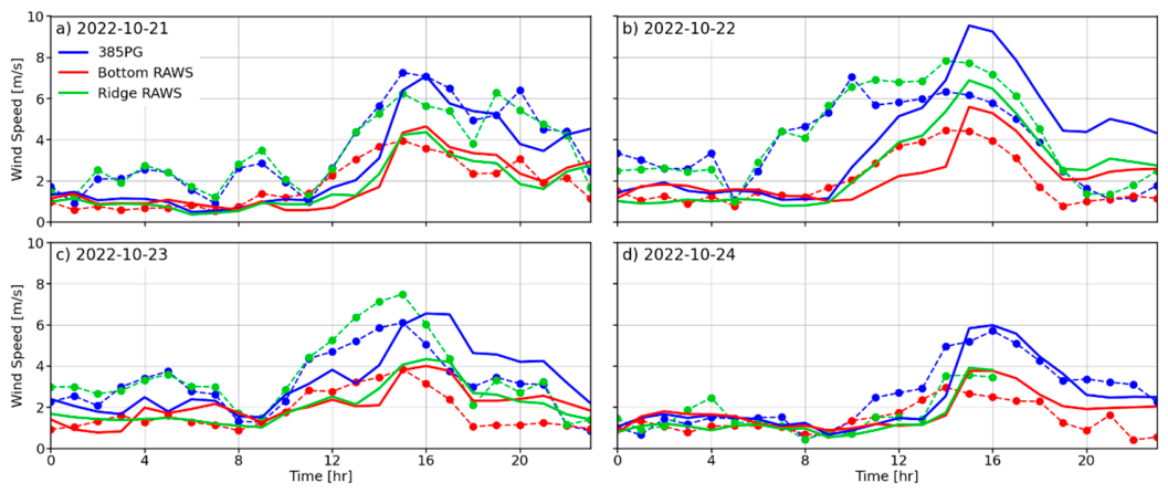
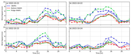
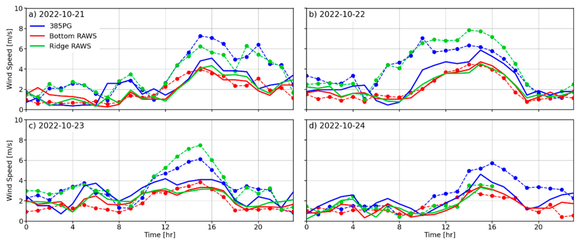
The WindNinja simulation results were evaluated against the observational data from each station at the sites of the Salinas and Feather River Canyon cases. We first evaluate WindNinja’s performance for simulations initialized from a singular point on the domain. Examining the results for wind speed (Figure 5) can see that the simulation curves closely follow the observed values for the Bottom RAWS throughout the days. We would expect simulation results for this station to be the best since the point initialization simulations for the Salinas case were initialized at the bottom of the canyon and thus closest to this station. The two stations, Ridge RAWS and 385PG, both located at the top of the canyon, delivered similar findings between the two of them. On several days, WindNinja underestimated wind speeds, which is especially shown in the afternoon hours. On 24 October, it was clear with low wind speeds, as observed in Figure 5d. On this day, the simulation results and observational data correspond the best for all stations out of the four days.

Figure 5. Time series of point initialization WindNinja simulations output for wind speed (solid lines) compared to observational data (dashed lines with markers) for three stations at the Salinas Canyon.

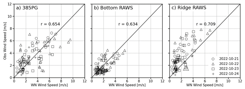
In Figure 6, correlation plots of wind speed with the observational data on the y-axis and the simulation output on the x-axis are depicted. Following diagonally through the plots, we have the identity line, which represents a perfect correlation between the simulation output and observations, and the different shapes represent the simulated days. The correlation plots between the WindNinja results and observations show the highest r-value for the Bottom RAWS station in Figure 6b. The Bottom RAWS is located at the bottom and inside the canyon and experienced lower wind speeds compared to the stations on the ridge crest, which is what we would expect. Since the model seems to struggle to predict higher wind speeds, the two ridge-top stations show lower r-scores and higher data spreads from the identity line. In Table 6, the MAE values are the lowest at the Bottom RAWS, which aligns with the previous findings in Figure 5. Examining all the stations of this case, we can conclude that WindNinja simulated wind speeds well, with the average MAE being just over 1 m s⁻¹ throughout all the simulated days.

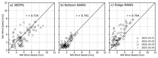
Figure 6. Correlation plots with r-values of wind speed for point initialization, WindNinja simulations output (horizontal axis), and observational data (vertical axis). The different symbols represent the four simulated days for three surface weather stations at the Salinas Canyon.

Table 6. Statistics for wind speed of point initialization simulations. Statistics calculated for all hours (r, MAE), morning between 5 and 11 AM (r (AM), MAE (AM)), and afternoon between 12 and 6 PM (r (PM), MAE (PM)). Calculated for all stations individually and over all stations of each site, which are highlighted in gray.

Site	Station	Site Descp.	r	r (AM)	r (PM)	MAE	MAE (AM)	MAE (PM)
Salinas	385PG	Ridge	0.698	0.443	0.747	1.781	1.622	2.068
	Bottom RAWS	Canyon	0.782	0.614	0.760	0.546	0.500	0.509
	Ridge RAWS	Ridge	0.733	0.506	0.773	1.108	1.258	0.990
	Avg					1.145	1.127	1.189
Feather	275PG	Ridge	0.072	0.441	0.627	11.882	10.096	16.929
	335PG	Canyon	0.097	0.686	0.636	5.800	6.512	6.198
	404PG	Valley	0.227	0.129	0.431	6.244	3.903	9.332
	PG129	Peak	−0.089	−0.033	0.232	15.491	13.990	20.732
	PG292	Valley	0.591	−0.044	0.493	6.750	5.137	8.646
	PG326	Ridge	0.599	0.231	0.857	12.708	10.648	17.730
	PG458	Valley	0.378	−0.264	0.049	7.583	6.508	9.944
	PG746	Peak	0.183	−0.229	0.773	11.279	9.697	15.160
	Avg					9.717	8.311	13.084

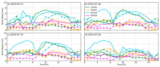
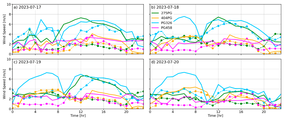
In Figure 7 and Figure 8, the point-initialized simulations for the Feather River Canyon case show that the model could not capture the wind speeds for the large domain well. WindNinja did not perform well at the northern and southern locations, and it overpredicted wind speeds throughout most of the day.

Figure 7. Time series of point initialization WindNinja simulations output for wind speed (solid lines) compared to observational data (dashed lines with markers) for the four stations in the northern part of the Feather River Canyon case.

Figure 8. Time series of point initialization WindNinja simulations output for wind speed (solid lines) compared to observational data (dashed lines with markers) for the four stations in the southern part of the Feather River Canyon case.

The correlation results in Figure 9 are thus not as good as in the Salinas Canyon case. Exceptionally low correlations are observed in Figure 9a,b,d. Due to the variability of the terrain and large domain size of the Feather River Canyon case site, we would not expect WindNinja to perform well with initialization from a singular point. Thus, these lower correlations were not surprising. As expected, the MAE values are significantly higher compared to the Salinas site. For the Feather River Canyon site, the average MAE of all stations is just under 10 m s⁻¹ (Table 6).

Figure 9. Correlation plots with r-values of wind speed for point initialization, WindNinja simulations output, and observational data. The different symbols represent the four simulated days for the eight PG&E stations of the Feather River Canyon case.

3.1.2. Wind Direction

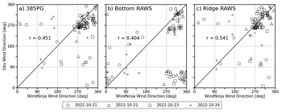
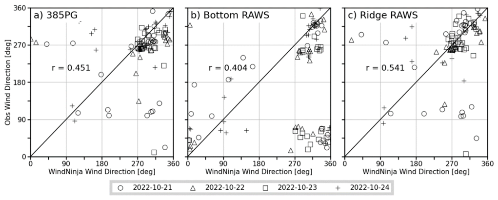
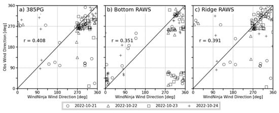
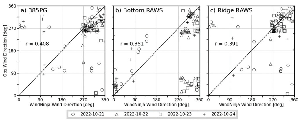
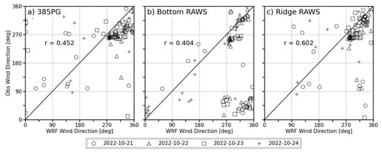
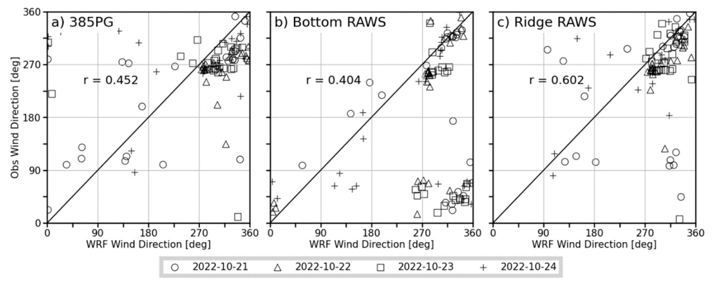
The previously discussed wind speed results of the Salinas Canyon site showed that WindNinja delivered slightly better results for the Bottom RAWS with the lower wind speeds that this station observed, nestled inside the canyon. However, wind direction at this location was difficult to simulate, whereas the simulations of the exposed ridge top stations were better due to better exposure to ambient wind flow above the canyon proper. Figure 10 shows that the two ridge stations in (a) and (c) have the best distribution between simulated and observed values, and also higher r-scores than the Bottom RAWS in (b). In the afternoon hours between 1200 and 1800 LT, the r values of all the stations are similar, ~0.67. As already noted, when it comes to looking at the MAE, the ridge-top stations performed generally better and showed a smaller error throughout the whole day. For the Salinas site, the average MAE is under 30°. In the afternoon, between 1200 and 1800 LT, when simulation results improve, the average MAE is only ~20° (Table 7).

Figure 10. Correlation plots with r-values of wind direction for point initialization WindNinja simulations output and observational data. The different symbols represent the four simulated days for three stations at the Salinas Canyon.

Table 7. Statistics for wind direction of point initialization simulations. Statistics calculated for all hours (r, MAE), morning between 5 and 11 AM (r (AM), MAE (AM)), and afternoon between 12 and 6 PM (r (PM), MAE (PM)). Calculated for all stations individually and over all stations of each site, which are highlighted in gray.

Site	Station	Site Descp.	r	r (AM)	r (PM)	MAE	MAE (AM)	MAE (PM)
Salinas	385PG	Ridge	0.461	0.196	0.662	27.124	30.529	22.153
	Bottom RAWS	Canyon	0.416	0.531	0.690	30.860	33.606	21.910
	Ridge RAWS	Ridge	0.500	0.289	0.646	23.758	29.711	18.216
	Avg					27.247	31.282	20.760
Feather	275PG	Ridge	−0.716	−0.706	−0.339	36.313	42.493	18.620
	335PG	Canyon	−0.067	−0.374	−0.553	29.475	30.600	39.548
	404PG	Valley	−0.797	−0.061	−0.850	23.240	33.506	10.484
	PG129	Peak	−0.656	−0.397	−0.091	32.155	31.740	34.312
	PG292	Valley	−0.149	−0.044	−0.300	30.841	28.828	23.606
	PG326	Ridge	−0.796	−0.443	−0.027	34.749	39.959	15.829
	PG458	Valley	−0.378	0.037	−0.033	41.221	48.646	45.279
	PG746	Peak	−0.661	−0.474	−0.189	25.278	24.404	18.396
	Avg					31.659	35.022	25.7593

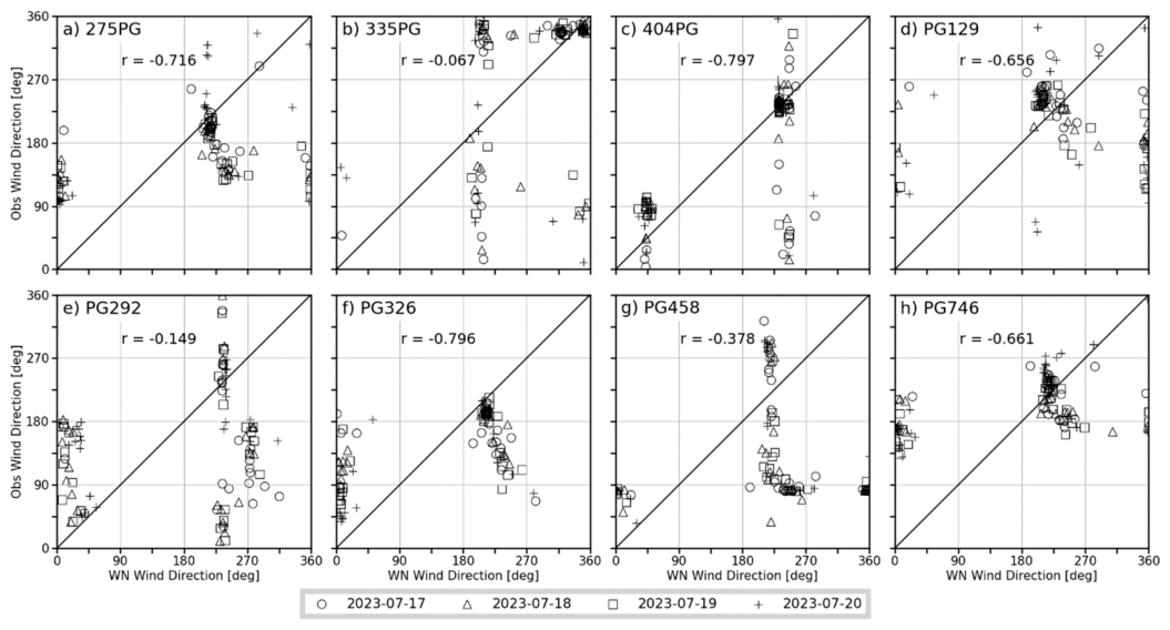
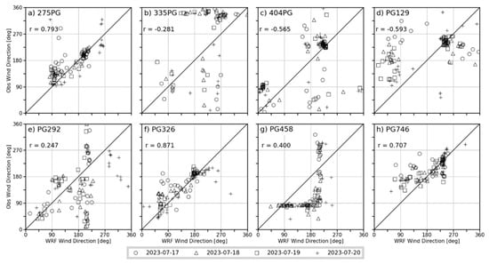
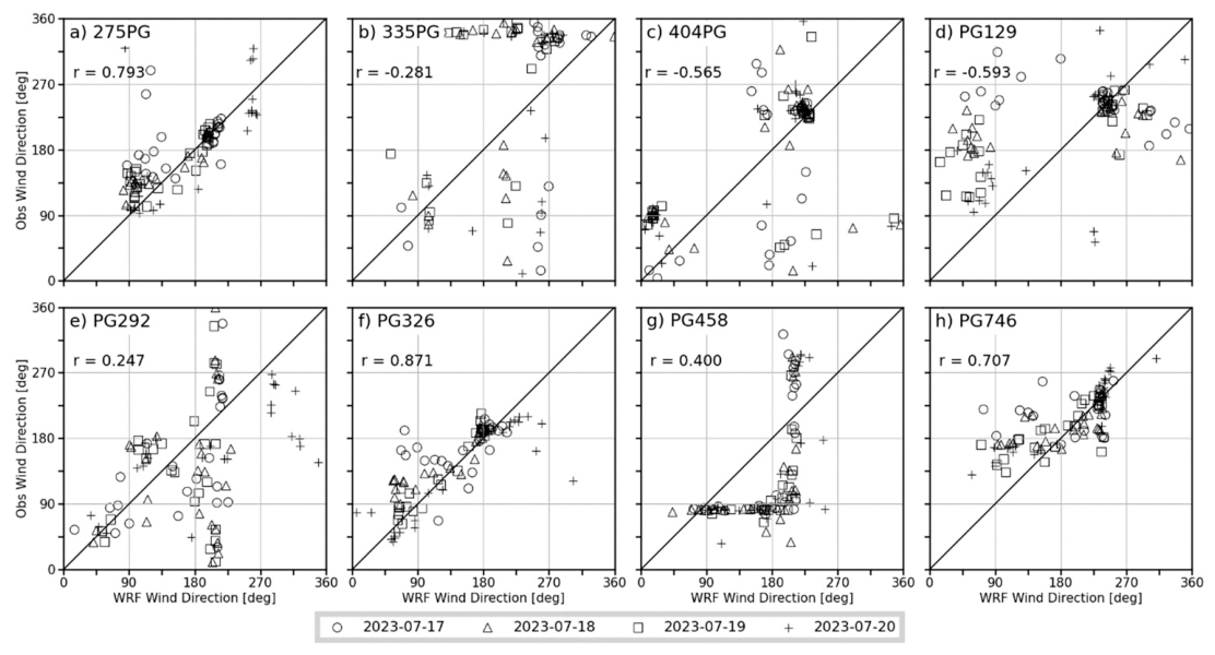
All the stations at the Feather River Canyon site show negative correlations (Figure 11). Out of the eight stations, five show a correlation coefficient lower than −0.5. As shown in Table 7, the majority of stations with stronger negative correlations, such as in (a), (d), (f), and (h) in Figure 11, are located on ridges or on mountaintops. The average MAE for all the stations in this domain is slightly over 30° and is similar to the average MAE at the Salinas site.

Figure 11. Correlation plots with r-values of wind direction for point initialization, WindNinja simulations output, and observational data. The different symbols represent the four simulated days for the eight PG&E stations of the Feather River Canyon case.

3.2. WindNinja Gridded Initialization

3.2.1. Wind Speed

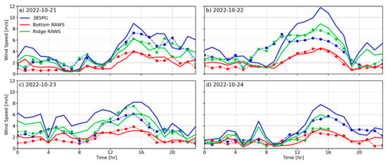
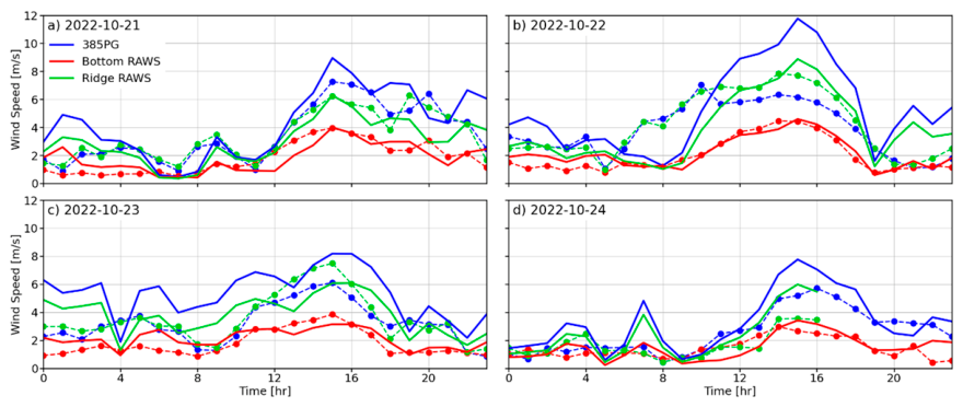
The following sets of simulations were done using WindNinja’s gridded initialization method, where 2 km gridded WRF data were downscaled to a resolution of 250 m. First, examining the Salinas Canyon case (Figure 12) again, the simulations yielded the best results across all four days for the location of the Bottom RAWS (red line). The results for the ridge-top stations are again not as good as those for the Bottom RAWS, especially after 1200 LT in Figure 12a–c, where larger differences between the simulated and observed wind speeds of the stations 385PG and Ridge RAWS are observed. Station 385PG shows better agreement with the observations than the Ridge RAWS but still has discrepancies in the morning hours. As shown for the point initialization case for the Salinas Canyon case, best results were observed for lower wind speed conditions (Figure 12d).

Figure 12. Time series of gridded initialization WindNinja simulations output for wind speed (solid lines) compared to observational data (dashed lines with markers) for three stations at the Salinas Canyon.

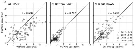
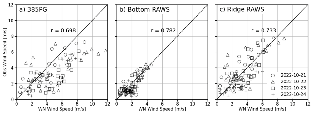
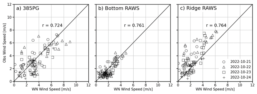
Figure 13 indicates higher correlation with r-values greater than 0.7 for all three stations. The ridge-top stations show an improvement in correlation coefficient values over their previous point initialization results. The Ridge RAWS station delivers the best r-values throughout the entire day and also when looking at the chosen morning and afternoon periods (Table 8). The average MAE also improved over the point initialization case and is now just under 1 m s⁻¹. These gridded initialization results align well with those of the point initialization Salinas case, despite the difference in mesh resolutions between the two initialization methods.

Figure 13. Correlation plots with r-values of wind speed for gridded initialization, WindNinja simulations output, and observational data. The different symbols represent the four simulated days for three stations at the Salinas Canyon.

Table 8. Statistics for wind speed of gridded initialization simulations. Statistics calculated for all hours (r, MAE), morning between 5 and 11 AM (r (AM), MAE (AM)), and afternoon between 12 and 6 PM (r (PM), MAE (PM)). Calculated for all stations individually and over all stations of each site, which are highlighted in gray.

Site	Station	Site Descp.	r	r (AM)	r (PM)	MAE	MAE (AM)	MAE (PM)
Salinas	385PG	Ridge	0.724	0.429	0.775	1.098	1.360	0.975
	Bottom RAWS	Canyon	0.761	0.477	0.706	0.611	0.583	0.615
	Ridge RAWS	Ridge	0.764	0.533	0.851	1.233	1.384	1.406
	Avg					0.981	1.109	0.999
Feather	275PG	Ridge	−0.068	0.043	0.654	1.962	1.510	3.634
	335PG	Canyon	0.238	0.156	0.484	0.731	0.500	0.863
	404PG	Valley	0.833	0.762	0.395	0.697	0.674	0.832
	PG129	Peak	−0.090	0.219	−0.088	2.899	1.601	5.346
	PG292	Valley	0.402	−0.216	0.613	0.794	1.070	0.635
	PG326	Ridge	0.445	0.232	0.795	1.765	2.685	1.004
	PG458	Valley	0.294	0.332	0.129	1.069	1.130	0.801
	PG746	Peak	0.400	0.342	0.809	1.284	0.850	2.247
	Avg					1.400	1.253	1.920

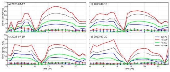
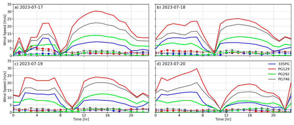
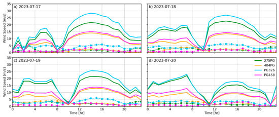
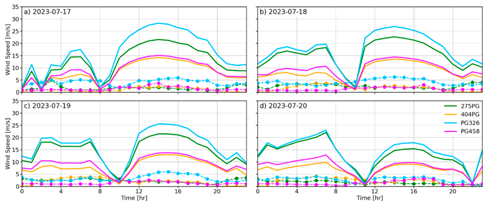
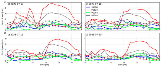
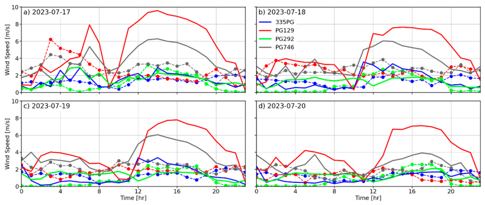
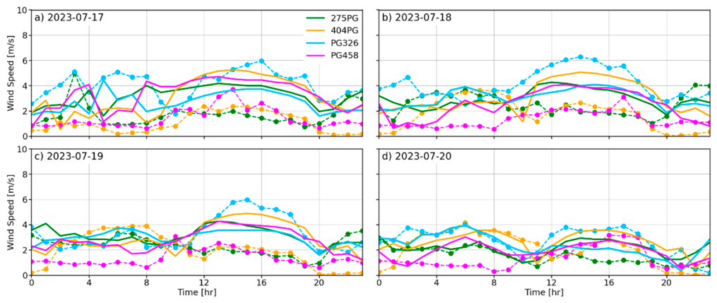
For the Feather River Canyon case (Figure 14 and Figure 15), the gridded initialization simulations deliver far better results than the point initialization (Figure 7). In this case, the simulated wind speeds are much closer to the observed values. As observed with the point-initialized simulations, WindNinja tends to overpredict wind speeds in the complex terrain of the Feather River Canyon case. However, the difference is not as extreme as it was for the point initialization simulations (Figure 7 and Figure 8). The high wind speeds observed in the afternoon, shown by the red and gray lines in Figure 14 and the green and blue lines in Figure 15, are for stations located on either peaks or ridges. Thus, the simulations tend to overpredict the observed wind speeds at these higher-elevation and more exposed locations.

Figure 14. Time series of gridded initialization WindNinja simulations output for wind speed (solid lines) compared to observational data (dashed lines with markers) for the four stations in the northern part of the Feather River Canyon case.

Figure 15. Time series of gridded initialization WindNinja simulations output for wind speed (solid lines) compared to observational data (dashed lines with markers) for the four stations in the southern part of the Feather River Canyon case.

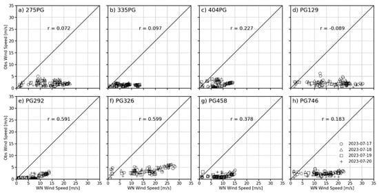
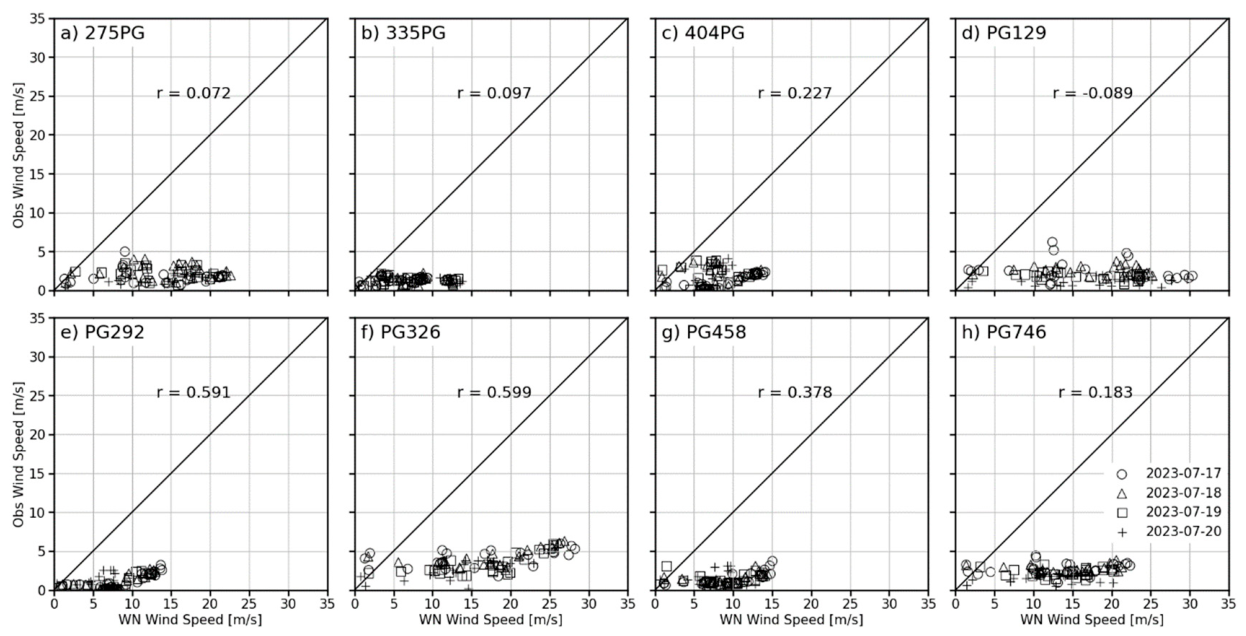
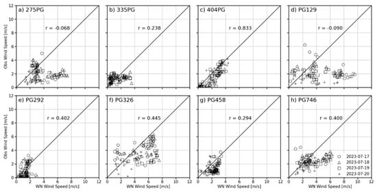
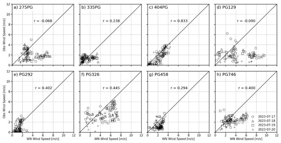
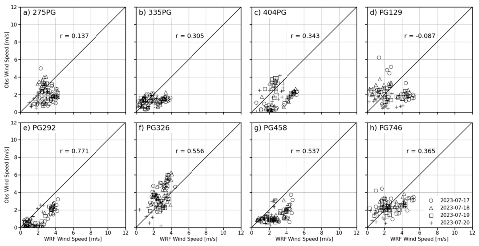
For the Feather River Canyon case, there are no drastic improvements using the gridded initialization compared to the point initialization (Figure 16). The stations in Figure 16c,h do show improvements in their correlations, but the stations in Figure 16e,f,h show decreases in their r-values. Stations in Figure 16a,d show almost no correlation using the gridded initialization method. Station 275PG is located on a ridge, and PG129 is located on a peak. Station 404PG, which is located in a valley at a lower elevation, had the best r-score. More exposed stations on peaks or ridges were associated with lower r-score values than stations in valleys or canyons (Table 8). Examining the average MAE values of all stations at the Feather River Canyon site (Table 8) indicates similarly low values to those of the Salinas site. For full day lengths, the average MAE is 1.4 m s⁻¹ for all stations. At this site, the average MAE for the morning period is better than the afternoon hours, which was not the case for the Salinas stations. The stations 275PG and PG129, which were also associated with poor r-scores close to 0, showed large MAE values in the afternoon. Overall, the MAE results are similar to those for the Salinas site.

Figure 16. Correlation plots with r-values of wind speed for gridded initialization WindNinja simulations output and observational data. The different symbols represent the four simulated days for the eight PG&E stations of the Feather River Canyon case.

3.2.2. Wind Direction

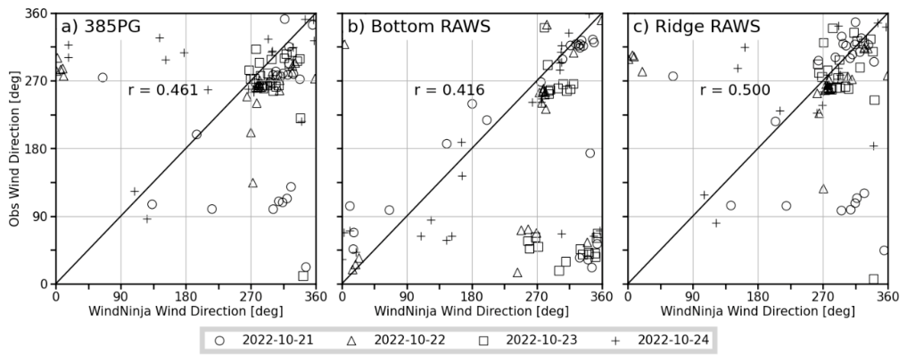
The wind direction correlations of the gridded WindNinja output (Figure 17) are very similar to the wind direction results of the point initialization output in Figure 10. The differences are smaller in the afternoon when the winds are less variable than in the morning hours. Same as with the point initialization case, the simulation output for the stations 385PG and Ridge RAWS correlates better with their respective observations than for the bottom RAWS. This is most likely due to the ridge stations being more exposed to the prevailing wind and not being confined by the topography of the canyon like the Bottom RAWS.

Figure 17. Correlation plots with r-values of wind direction for gridded initialization WindNinja simulations output and observational data. The different symbols represent the four simulated days for three stations at the Salinas Canyon.

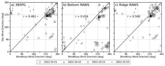
Stations 385PG (Figure 17a) and Ridge RAWS (Figure 17b) show the most consistent distributions, with wind directions being mostly around 270–320°. For the Bottom RAWS, the directions are more scattered and range from ~300 to 90°. The correlation coefficient for this station is also lower compared to the ridge stations. Overall, the ridge-top stations show lower correlation coefficients in the morning and higher ones in the afternoon hours (Table 9). The Bottom RAWS shows the opposite, with r-values being higher for the AM hours and lower during the PM ones. This finding was also seen in the point initialization wind directions. When looking at MAE values, the average error is less than 30° across all stations for the full days. The MAE of the ridge stations is even better and in the range of 22–25°. As expected, the MAE values are higher in the AM and lower in the PM. As seen before, the results for the Bottom RAWS are slightly worse, around 30° or upward from there.

Table 9. Statistics for wind direction of gridded initialization simulations. Statistics calculated for all hours (r, MAE), morning between 5 and 11 AM (r (AM), MAE (AM)), and afternoon between 12 and 6 PM (r (PM), MAE (PM)). Calculated for all stations individually and over all stations of each site, which are highlighted in gray.

Site	Station	Site Descp.	r	r (AM)	r (PM)	MAE	MAE (AM)	MAE (PM)
Salinas	385PG	Ridge	0.451	0.322	0.475	25.115	29.849	20.372
	Bottom RAWS	Canyon	0.404	0.619	0.410	34.717	37.729	29.001
	Ridge RAWS	Ridge	0.541	0.381	0.509	22.717	28.060	17.275
	Avg					27.516	31.879	22.216
Feather	275PG	Ridge	0.800	0.745	0.626	21.743	25.292	11.173
	335PG	Canyon	−0.204	−0.002	−0.123	37.916	36.774	37.228
	404PG	Valley	0.809	0.403	−0.276	27.168	36.618	21.101
	PG129	Peak	−0.472	0.073	0.154	27.202	39.367	8.455
	PG292	Valley	0.293	−0.013	−0.183	37.870	43.707	32.401
	PG326	Ridge	0.836	0.741	0.612	24.285	26.291	7.641
	PG458	Valley	0.375	−0.024	0.550	46.950	45.269	45.789
	PG746	Peak	0.703	0.359	0.499	28.155	29.894	21.297
	Avg					31.411	35.402	23.136

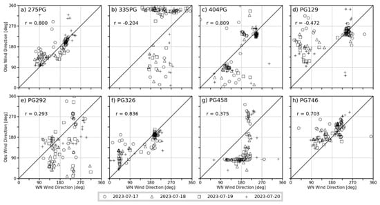
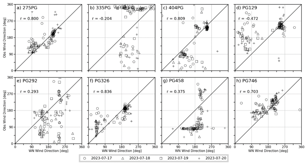
The correlation coefficient results for the Feather River Canyon (Figure 18) show significant improvement with the gridded initialization method. Stations with high agreement between simulated and observed directions (Figure 18a,c,f,h) also show high correlations in their r-scores. Three of those four stations show a higher r-score in the AM than in the PM. This is astonishing since lower correlations would be expected when the winds are more variable (Table 9) during the typical morning transition period. MAE values did not change much compared to the previous results of the point initialization case. Over the whole day, the average MAE for all stations is ca. 31°. During the AM period, the average MAE is ca. 35°, and during the PM, it is ca. 23°. The values over the entire day and in the morning hours are very close to those for the point initialization case. The average MAE PM value improved slightly. In Table 9, larger MAE values are observed at stations located in valley or canyon topography, such as with 335PG, PG292, and PG458. These stations are located in areas more confined by the surrounding higher terrain. Their MAE values are larger by at least 10° compared to the stations at more exposed areas, such as on ridges or peaks.

Figure 18. Correlation plots with r-values of wind direction for gridded initialization, WindNinja simulations output, and observational data. The different symbols represent the four simulated days for the eight PG&E stations of the Feather River Canyon case.

3.3. WindNinja Conservation of Mass and Momentum Solver

3.3.1. Wind Speed

The following comparisons for WindNinja’s mass and momentum solver are limited to the Salinas Canyon case site. Comparing the gridded initialized simulations using the mass and momentum conserving solver for the Salinas site (Figure 19) with the previous simulations using only the mass-conserving solver in (Figure 12), we again see the best match of simulation output to observations is for the Bottom RAWS. The two ridge stations show greater differences, which is especially visible in the afternoon when the wind speeds pick up. Looking at the day of the experiment in Figure 19d, WindNinja simulated the wind speeds very well in the AM, even better than the previous gridded simulations (Figure 12). In the PM, the results of the two solvers are similar, showing smaller discrepancies between the model output and observations.

Figure 19. Time series of gridded initialization WindNinja simulations output for wind speed (solid lines) compared to observational data (dashed lines with markers) for three stations at the Salinas Canyon. These simulations used the model’s conservation of mass and momentum solver.

Comparing correlations (Figure 13 and Figure 20) shows that the r-scores are lower at each station for the simulations using the conservation of mass and momentum solver. Also noticeable is a larger spread of the data from the 1:1 line, and the station (Figure 20b) delivers the lowest correlation coefficient of the three stations. When only focusing on the timeframe 5 through 11 LT, we see an improvement in the ridge stations’ r-scores of 0.1 (Table 10). However, the Bottom RAWS did score lower with these new simulations. For the PM period, lower r-scores are observed at all stations when comparing them to the results in Table 8, where the Bottom RAWS has a much lower correlation coefficient during these afternoon times, with a decrease of over 0.3. The MAEs have also increased slightly when looking at the whole day, and also only during the PM hours. In the PM, we have the largest increase in errors, which is due to the higher wind speeds during those hours. For the AM, the MAE average across all stations only improves by a fraction. Overall though, for this site, the simulation results did not improve using WindNinja’s more advanced solver, and the previous simulations using only the native solver delivered, in most cases, higher r-scores and lower MAE values.

Figure 20. Correlation plots with r-values of wind speed for gridded initialization, WindNinja simulations output, and observational data. The different symbols represent the four simulated days for three stations at the Salinas Canyon. These simulations used the model’s conservation of mass and momentum solver.

Table 10. Statistics for wind speed of mass and momentum simulations. Statistics calculated for all hours (r, MAE), morning between 5 and 11 AM (r (AM), MAE (AM)), and afternoon between 12 and 6 PM (r (PM), MAE (PM)). Calculated for all stations individually and over all stations (highlighted in gray) of the Salinas Canyon site.

Site	Station	Site Descp.	r	r (AM)	r (PM)	MAE	MAE (AM)	MAE (PM)
Salinas	385PG	Ridge	0.654	0.545	0.591	1.242	1.221	1.392
	Bottom RAWS	Canyon	0.634	0.413	0.382	0.776	0.423	1.131
	Ridge RAWS	Ridge	0.709	0.639	0.700	1.493	1.586	1.723
	Avg					1.170	1.077	1.415

3.3.2. Wind Direction

The correlation plots in Figure 21 show us lower r-scores for the three stations when using WindNinja’s newer and more advanced solver. In comparison, the simulations using only the mass-conserving solver delivered better correlation values for all the stations, as seen in Figure 17. The distribution of the data in Figure 21 is very similar to the distribution of the previous results, with the greatest amount of data concentrated around 270–320° for the stations in Figure 21a,c. Also, when splitting up the hours for the AM and PM analysis in Table 11, there is a decrease in the r-scores compared to the native solver’s results in Table 9. The Bottom RAWS station shows a decent correlation of over 0.5 in the AM but a correlation coefficient close to 0 for the PM times. Moving on to the MAE statistics, higher MAE values can be seen as well. The differences between the results of the two simulation types are small; however, the mass- and momentum-conserving simulations consistently delivered higher MAE values by 2°. This is a marginal increase; however, better or at least equal results with WindNinja’s more complex and improved solver compared to its native one were expected.

Figure 21. Correlation plots with r-values of wind direction for gridded initialization, WindNinja simulations output, and observational data. The different symbols represent the four simulated days for three stations at the Salinas Canyon. These simulations used the model’s conservation of mass and momentum solver.

Table 11. Statistics for wind direction of mass and momentum simulations. Statistics calculated for all hours (r, MAE), morning between 5 and 11 AM (r (AM), MAE (AM)), and afternoon between 12 and 6 PM (r (PM), MAE (PM)). Calculated for all stations individually and over all stations (highlighted in gray) of the Salinas Canyon site.

Site	Station	Site Descp.	r	r (AM)	r (PM)	MAE	MAE (AM)	MAE (PM)
Salinas	385PG	Ridge	0.408	0.164	0.242	27.547	35.819	23.826
	Bottom RAWS	Canyon	0.351	0.563	0.097	35.305	38.197	32.077
	Ridge RAWS	Ridge	0.391	0.182	0.266	24.694	31.085	21.786
	Avg					29.182	35.034	25.896

3.4. WRF Output Comparison

3.4.1. Wind Speed

Lastly, the WRF output for the specific stations and their respective observations is analyzed to see how the WRF and WindNinja simulation outputs compare. In Figure 22, we have the best agreement for the Bottom RAWS again. The two ridge-top stations show larger discrepancies, the same as for the WindNinja simulations. However, in the case of the WRF data, the model underpredicts wind speeds throughout most of the day for these two stations. The gridded initialization simulations’ wind speeds in Figure 12 show that WindNinja predicted wind speeds closer to the observations, or in the case of station 385PG, even overpredicted wind speeds during certain times of the day. This does not occur with the WRF results (Figure 22).

Figure 22. Time series of WRF output for wind speed (solid lines) compared to observational data (dashed lines with markers) for three stations at the Salinas Canyon.

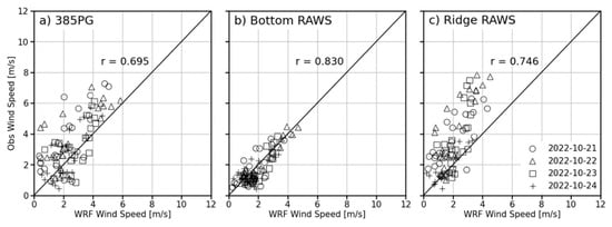
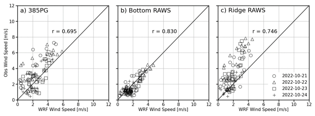
The correlation plots for the WRF data to observations show the highest r-score for the Bottom RAWS (Figure 23b). This r-score is higher than the point initialization or gridded initialization results for this station. The wind speeds are closer to the 1:1 line than for the WindNinja simulation results. In the case of the ridge stations, the correlation coefficient values are slightly lower compared to the WindNinja results (Table 8). For the AM and PM r-values, lower correlations can be seen in the AM and higher correlations in the PM, as seen in the previous statistics. Out of the three Salinas Canyon stations, only the Bottom RAWS showed better correlations when only using WRF, and the ridge stations improved slightly with the WindNinja simulations. The MAE values for this site are very close to the ones received previously. In Table 12, the average MAE values are just over 1 m s⁻¹. The same as seen with the r-values before, the MAE results for the Bottom RAWS were better with WRF than with WindNinja. On the other hand, the MAE values of the ridge stations are higher than they were with WindNinja. The differences between WRF and WindNinja MAE values are small though, with WindNinja improving the wind speed values only by ca. 0.1 m s⁻¹ when looking at the entire day.

Figure 23. Correlation plots with r-values of wind speed for WRF output and observational data. The different symbols represent the four simulated days for three stations at the Salinas Canyon.

Table 12. Statistics of wind speed for WRF. Statistics calculated for all hours (r, MAE), morning between 5 and 11 AM (r (AM), MAE (AM)), and afternoon between 12 and 6 PM (r (PM), MAE (PM)). Calculated for all stations individually and over all stations of each site, which are highlighted in gray.

Site	Station	Site Descp.	r	r (AM)	r (PM)	MAE	MAE (AM)	MAE (PM)
Salinas	385PG	Ridge	0.695	0.396	0.802	1.239	1.252	1.342
	Bottom RAWS	Canyon	0.830	0.702	0.795	0.505	0.472	0.494
	Ridge RAWS	Ridge	0.746	0.535	0.764	1.463	1.312	2.129
	Avg					1.069	1.012	1.322
Feather	275PG	Ridge	0.137	0.204	0.662	1.168	0.844	1.895
	335PG	Canyon	0.305	0.152	0.571	0.907	0.683	1.556
	404PG	Valley	0.343	0.212	0.412	1.644	1.159	2.282
	PG129	Peak	−0.087	0.242	0.091	1.595	1.193	2.580
	PG292	Valley	0.771	0.537	0.550	1.053	0.759	1.152
	PG326	Ridge	0.556	0.402	0.882	1.117	0.727	1.640
	PG458	Valley	0.537	0.412	−0.021	1.333	1.478	1.575
	PG746	Peak	0.365	0.295	0.798	0.991	0.857	1.314
	Avg					1.226	0.963	1.749

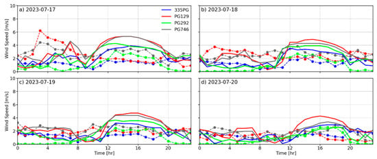
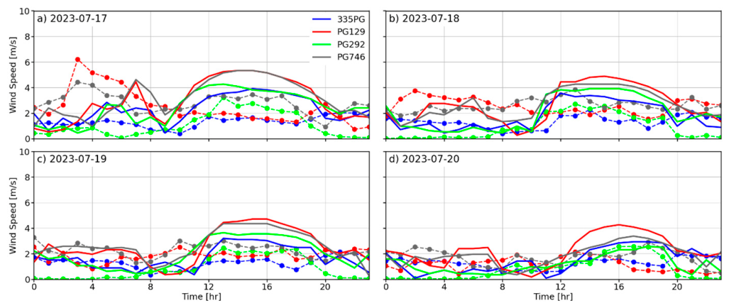
Figure 24 and Figure 25, showing the WRF output for the Feather River Canyon, indicate a less drastic increase in wind speed in the afternoon for certain stations than WindNinja did (Figure 14 and Figure 15). WRF still overpredicts wind speeds, but the difference to the observations is not as stark as with WindNinja. In Figure 22 for the Salinas case, WRF underpredicted wind speeds in the PM, whereas for the Feather River Canyon case, WRF slightly overpredicted wind speeds for most stations in Figure 24 and Figure 25.

Figure 24. Time series of WRF output for wind speed (solid lines) compared to observational data (dashed lines with markers) for the four stations located in the northern part of the Feather River Canyon case.

Figure 25. Time series of WRF output for wind speed (solid lines) compared to observational data (dashed lines with markers) for the four stations located in the southern part of the Feather River Canyon case.

Comparing the correlation plots of WRF for the Feather River Canyon in Figure 26 to the ones of the gridded WindNinja simulations in Figure 16 shows that for most stations, correlations are better with WRF than with WindNinja. Only stations in Figure 26c,h show lower r-scores with WRF. The scattering is also closer to the 1:1 line for most stations with the WRF results than with WindNinja. In Table 12 for the AM values, WRF has better correlations for all stations besides one when comparing them to WindNinja’s statistics (Table 8). For the PM values, the WRF values align more with the WindNinja results. Continuing with the MAE values, WRF consistently delivered better values when looking at all MAE tests (Table 12) compared to the WindNinja values in Table 8. The difference is not big, and WRF’s average MAE for the whole day and PM hours is ca. 0.2 m s⁻¹ better. For the AM times, WRF’s MAE average is ca. 0.3 m s⁻¹ better than the WindNinja results. The WindNinja results showed a larger MAE in the PM for certain stations; for example, PG129, where the MAE was greater than 5 m s⁻¹. The WRF results did not show such high errors, and PG129 has an MAE of ca. 2.5 m s⁻¹ s in the PM. Overall, WRF delivered better wind speed statistics for the Feather River Canyon than WindNinja.

Figure 26. Correlation plots with r-values of wind speed for WRF output and observational data. The different symbols represent the four simulated days for the eight PG&E stations of the Feather River Canyon case.

3.4.2. Wind Direction

The first noticeable similarity between the WRF wind direction correlation coefficient results in Figure 27 and those of WindNinja in Figure 17 is that the r-scores of the stations in Figure 27a,b are the same. The correlation coefficient for Figure 27c improved with the WRF data. Overall, the wind direction correlation plots for WRF and those for WindNinja are very similar. Across the statistical tests, Table 13 shows higher r-values by about 0.1 for the ridge stations compared to the values for WindNinja in Table 9. In the PM hours, the r-scores of all three stations are higher when using WRF, especially for the Bottom RAWS, where the correlation coefficient increases by ca. 0.3. The MAE values in Table 13 are not as good as the results with WindNinja. Again, the differences are small, and when looking at the entire day, WindNinja’s MAE outperformed WRF by only 2°. WindNinja delivered better results for the exposed ridge-top stations. For example, its MAE for station 385PG is 7° smaller than WRF’s for this specific station. However, when it comes to the Bottom RAWS, which is nestled inside the canyon, WRF performed better.

Figure 27. Correlation plots with r-values of wind direction for WRF output and observational data. The different symbols represent the four simulated days for three stations at the Salinas Canyon.

Table 13. Statistics for wind direction of WRF. Statistics calculated for all hours (r, MAE), morning between 5 and 11 AM (r (AM), MAE (AM)), and afternoon between 12 and 6 PM (r (PM), MAE (PM)). Calculated for all stations individually and over all stations of each site, which are highlighted in gray.

Site	Station	Site Descp.	r	r (AM)	r (PM)	MAE	MAE (AM)	MAE (PM)
Salinas	385PG	Ridge	0.452	0.440	0.564	32.659	34.883	28.051
	Bottom RAWS	Canyon	0.404	0.394	0.705	31.511	35.936	21.794
	Ridge RAWS	Ridge	0.602	0.485	0.534	25.174	27.585	23.843
	Avg					29.781	32.801	24.563
Feather	275PG	Ridge	0.793	0.701	0.883	21.651	22.012	12.150
	335PG	Canyon	−0.281	−0.396	−0.265	39.745	29.371	43.140
	404PG	Valley	−0.565	−0.390	−0.517	33.778	44.336	17.875
	PG129	Peak	−0.593	−0.147	−0.414	28.565	37.797	10.949
	PG292	Valley	0.247	0.298	−0.632	34.221	31.077	31.785
	PG326	Ridge	0.871	0.774	0.605	20.975	19.212	13.475
	PG458	Valley	0.400	−0.096	0.557	41.702	34.515	46.734
	PG746	Peak	0.707	0.455	0.694	25.595	33.213	9.493
	Avg					30.779	31.442	23.200

The correlation plots for WRF in Figure 28 are comparable to the ones for WindNinja in Figure 18. For some of the stations, WRF delivered better correlations, but in most instances, WindNinja outperformed WRF, even though the differences were not always large. The one case where WindNinja’s better correlations stand out is at station 404PG in c). In this case, WindNinja has a strong positive correlation of ca. 0.8, whereas WRF is negatively correlated with an r-score of ca. −0.57. In the AM, the WRF r-values are better than WindNinja’s. Four out of the eight stations of this site had a correlation coefficient very close to 0 with WindNinja (Table 9). When comparing those to the r-scores of WRF, only one of the stations has an r-score close to 0. In the PM hours, WRF has higher correlations to the observations than WindNinja did. The stations that exhibit positive correlations are closer between WRF and WindNinja than stations that show negative correlations. For those stations, we see stronger negative correlations for WRF than we did for WindNinja. Looking at the MAE values for the wind direction of WRF, we have values that are slightly better than those of WindNinja. Same as seen with the Salinas Canyon site, the differences are minuscule, this time being under 1° difference. For the AM values, WRF’s better performance compared to WindNinja’s becomes more evident, with the difference between the MAEs now being 4°. However, in the afternoon, when the winds are not as variable, the results of the two models are practically the same.

Figure 28. Correlation plots with r-values of wind direction for WRF output and observational data. The different symbols represent the four simulated days for the eight PG&E stations of the Feather River Canyon case.

4. Discussion and Conclusions

This study evaluated WindNinja’s performance over highly complex terrain with canyons. The validation was conducted at two case sites, with different numerical solvers and different initialization methods of the diagnostic model. Further, WindNinja’s results were compared to the WRF model’s output to see if WindNinja could improve upon the mesoscale model’s forecast in a canyon setting.

Between the point and gridded initialization methods of WindNinja, the latter method delivered better results for both cases when it came to the simulation of wind speed. However, for the Salinas site with simpler terrain, the results of the two initialization methods are similar, with the gridded initialization method showing improvements in the wind speed of the ridge-top stations. The poor performance of the point initialization for the Feather River Canyon case is not surprising, since this site is made up of highly variable terrain and a large domain size. This case tested the limitations of WindNinja’s point initialization and showed that this method may be a reasonable approximation when dealing with small domains. However, gridded initialization is more appropriate for larger domains with heterogeneous terrain. Across both case sites, WindNinja showed the largest wind speed MAE for stations located on peaks or ridges, demonstrating that WindNinja struggled to simulate the higher wind speeds occurring at those locations. When it came to results for wind direction, there was not a large difference between the different initialization methods at either of the two sites. However, the results still improved marginally using the gridded initialization method with an average wind direction MAE of around 30° across all stations. Contrary to the wind speed results, the highest MAE for wind direction occurred at stations located in valleys or canyons. The model did capture well the recirculation occurring in valleys or canyons because these WindNinja simulations were conducted with the native solver, which does not account for the conservation of momentum. Stations located on exposed peaks or ridges were easier to simulate in terms of wind direction.

Using WindNinja’s more advanced conservation of mass and momentum solver over the native conservation of mass solver did not improve the simulation results at the Salinas site. At the Salinas site, with its simpler terrain, lower correlation values and higher MAEs were found for both wind speed and wind direction when using the mass and momentum conserving solver over the native solver. WindNinja’s mass and momentum conserving simulations also required more computing power and took roughly three times longer to simulate than the solely mass-conserving simulations. The advanced solver worked adequately when running simulations of our domain sizes. However, these simulations are not an option for entities such as utility companies or land management agencies that wish to cover their entire service areas.

When comparing the gridded WindNinja output to WRF output, WindNinja did not show big improvements over the mesoscale model’s forecast. This was especially the case for the Feather River Canyon, where we received better results only using WRF. These results over highly complex and variable terrain correspond with the findings of Wagenbrenner et al. [28], where WindNinja could not simulate the microscale processes around terrain; however, our two cases cannot be generalized to all areas of complex terrain. One of the reasons for WindNinja’s poorer results compared to WRF’s could relate to the fact that WindNinja’s governing equations assume incompressible flow, while WRF’s governing equations assume compressible flow. This means WindNinja could not account for variability in air density related to altitude changes; for example, over the complex domain of the Feather River Canyon site. The terrain complexity would also explain why WindNinja delivered better results for the Salinas Canyon case, which is surrounded by much simpler terrain. Thus, the wind flow patterns are not altered as much by changes in topography as they were in the Feather River Canyon.

In conclusion, WindNinja generally delivered better results for simulations conducted over the Salinas Canyon site with simpler terrain and slightly improved upon the WRF forecast, which was used as WindNinja’s input. However, for the Feather River Canyon with its more complex terrain and very deep and winding canyons, WindNinja delivered poorer results, especially at stations on ridges or peaks where wind speeds tend to be higher in magnitude. In those instances, only using the WRF output delivered a more accurate forecast. However, our conclusions should be taken with caution and should not be generalized for all cases and terrain types. Our study is limited because we only tested two sites with complex terrain and thus, our results represent only those two cases. To truly assess the performance of WindNinja, additional case studies are needed to ascertain model performance across various wind regimes and canyon geometries. Future work should also further analyze WindNinja’s capabilities at high wind speeds, as past studies have indicated that the model performs better in those conditions. These analyses would help practitioners understand the model’s performance and limitations during high-wind events in regions of complex terrain.

References

- Viegas, D.X.; Simeoni, A. Eruptive Behavior of Forest Fires. Fire Technol. 2010, 47, 303–320. [Google Scholar] [CrossRef] [Scilit]
- Viegas, D.X. A mathematical model for forest fires blowup. Combust. Sci. Technol. 2005, 177, 27–51. [Google Scholar] [CrossRef] [Scilit]
- Xie, X.; Liu, N.; Raposo, J.R.; Viegas, D.X.; Yuan, X.; Tu, R. An experimental and analytical investigation of canyon fire spread. Combust. Flame 2020, 212, 367–376. [Google Scholar] [CrossRef] [Scilit]
- Sharples, J.J. Review of mountain meteorological effects relevant to fire behaviour and bushfire risk. Int. J. Wildland Fire 2009, 18, 737–754. [Google Scholar] [CrossRef] [Scilit]
- Werth, P.A.; Potter, B.E.; Clements, C.B.; Finney, M.A.; Forthofer, J.A.; McAllister, S.S.; Goodrick, S.L.; Alexander, M.E.; Cruz, M.G. Effects of complex terrain on extreme fire behavior. In Synthesis of Knowledge of Extreme Fire Behavior: Volume 1 for Fire; General Technical Report PNW-GTR-854; U.S. Department of Agriculture, Forest Service: Portland, OR, USA, 2011; pp. 5–19. [Google Scholar]
- Abatzoglou, J.T.; Kolden, C.A.; Williams, A.P.; Sadegh, M.; Balch, J.K.; Hall, A. Downslope wind-driven fires in the western United States. Earth’s Futur. 2023, 11, e2022EF003471. [Google Scholar] [CrossRef] [Scilit]
- Whiteman, C.D. Mountain Meteorology: Fundamentals and Applications; Oxford University Press: New York, NY, USA, 2000; 355p. [Google Scholar]
- Walmsley, J.L.; Taylor, P.A. Boundary-layer flow over topography: Impacts of the Askervein study. Bound. Layer Meteorol. 1996, 78, 291–320. [Google Scholar] [CrossRef] [Scilit]
- Jensen, N.O.; Peterson, E.W. On the escarpment wind profile. Q. J. R. Meteorol. Soc. 1978, 104, 719–728. [Google Scholar] [CrossRef]
- Taylor, P.A.; Mason, P.J.; Bradley, E.F. Boundary-layer flow over low hills. Bound. Layer Meteorol. 1987, 39, 107–132. [Google Scholar] [CrossRef] [Scilit]
- Taylor, P.A.; Teunissen, H.W. The Askervein Hill project: Overview and background data. Bound. Layer Meteorol. 1987, 39, 15–39. [Google Scholar] [CrossRef] [Scilit]
- Hunt, J.C.R.; Leibovich, S.; Richards, K.J. Turbulent shear flows over low hills. Q. J. R. Meteorol. Soc. 1988, 114, 1435–1470. [Google Scholar] [CrossRef]
- Forthofer, J.M.; Butler, B.W.; Wagenbrenner, N.S. A comparison of three approaches for simulating fine-scale surface winds in support of wildland fire management. Part I. Model formulation and comparison against measurements. Int. J. Wildland Fire 2014, 23, 969–981. [Google Scholar] [CrossRef] [Scilit]
- Skamarock, W.C.; Klemp, J.; Dudhia, J.; Gill, D.O.; Barker, D.; Duda, M.G.; Huang, X.-Y.; Wang, W.; Powers, J.G. A Description of the Advanced Research WRF Version 3; NCAR Technical Note NCAR/TN-475+STR; University Corporation for Atmospheric Research: Boulder, CO, USA, 2008; 113p. [Google Scholar] [CrossRef] [Scilit]
- Li, S.; Sun, X.; Zhang, S.; Zhao, S.; Zhang, R. A study on microscale wind simulations with a coupled WRF-CFD model in the chongli mountain region of hebei province, China. Atmosphere 2019, 10, 731. [Google Scholar] [CrossRef] [Scilit]
- Schär, C.; Leuenberger, D.; Fuhrer, O.; Lüthi, D.; Girard, C. A new terrain-following vertical coordinate formulation for atmospheric prediction models. Mon. Weather Rev. 2002, 130, 2459–2480. [Google Scholar] [CrossRef] [Scilit]
- Zängl, G.; Gantner, L.; Hartjenstein, G.; Noppel, H. Numerical errors above steep topography: A model intercomparison. Meteorol. Z. 2004, 13, 69–76. [Google Scholar] [CrossRef] [Scilit]
- Jiménez, P.A.; Dudhia, J. Improving the representation of resolved and unresolved topographic effects on surface wind in the wrf model. J. Appl. Meteorol. Climatol. 2012, 51, 300–316. [Google Scholar] [CrossRef] [Scilit]
- Jiménez, P.A.; Dudhia, J. On the ability of the WRF model to reproduce the surface wind direction over complex terrain. J. Appl. Meteorol. Climatol. 2013, 52, 1610–1617. [Google Scholar] [CrossRef] [Scilit]
- Jiménez, P.A.; Dudhia, J.; González-Rouco, J.F.; Montávez, J.P.; García-Bustamante, E.; Navarro, J.; Vilà-Guerau De Arellano, J.; Muñoz-Roldán, A. An evaluation of WRF’s ability to reproduce the surface wind over complex terrain based on typical circulation patterns. J. Geophys. Res. Atmos. 2013, 118, 7651–7669. [Google Scholar] [CrossRef] [Scilit]
- Lundquist, K.A.; Chow, F.K.; Lundquist, J.K. An immersed boundary method for the weather research and forecasting model. Mon. Weather Rev. 2010, 138, 796–817. [Google Scholar] [CrossRef] [Scilit]
- Lundquist, K.A.; Chow, F.K.; Lundquist, J.K. An immersed boundary method enabling large-eddy simulations of flow over complex terrain in the wrf model. Mon. Weather Rev. 2012, 140, 3936–3955. [Google Scholar] [CrossRef] [Scilit]
- Ma, Y.; Liu, H. Large-Eddy Simulations of Atmospheric Flows Over Complex Terrain Using the Immersed-Boundary Method in the Weather Research and Forecasting Model. Bound. Layer Meteorol. 2017, 165, 421–445. [Google Scholar] [CrossRef] [Scilit]
- Forthofer, J.M.; Butler, B.W.; Mchugh, C.W.; Finney, M.A.; Bradshaw, L.S.; Stratton, R.D.; Shannon, K.S.; Wagenbrenner, N.S. A comparison of three approaches for simulating fine-scale surface winds in support of wildland fire management. Part II. An exploratory study of the effect of simulated winds on fire growth simulations. Int. J. Wildland Fire 2014, 23, 982–994. [Google Scholar] [CrossRef] [Scilit]
- Chen, G.; Xiong, Q.; Morris, P.J.; Paterson, E.G.; Sergeev, A.; Wang, Y.-C. OpenFOAM for Computational Fluid Dynamics. Not. Am. Math. Soc. 2014, 61, 354–363. [Google Scholar] [CrossRef] [Scilit]
- Seto, D.; Jones, C.; Siuta, D.; Wagenbrenner, N.; Thompson, C.; Quinn, N. Evaluation of HRRR Wind Speed Forecast and WindNinja Downscaling Accuracy during Santa Ana Wind Events in Southern California. Weather Forecast. 2025, 40, 525–541. [Google Scholar] [CrossRef] [Scilit]
- Wagenbrenner, N.S.; Forthofer, J.M.; Page, W.G.; Butler, B.W. Development and evaluation of a reynolds-averaged navier-stokes solver in windninja for operational wildland fire applications. Atmosphere 2019, 10, 672. [Google Scholar] [CrossRef] [Scilit]
- Wagenbrenner, N.S.; Forthofer, J.M.; Lamb, B.K.; Shannon, K.S.; Butler, B.W. Downscaling surface wind predictions from numerical weather prediction models in complex terrain with WindNinja. Atmos. Chem. Phys. 2016, 16, 5229–5241. [Google Scholar] [CrossRef] [Scilit]
- Missoula Fire Sciences Laboratory. WindNinja Tutorial 2: Diurnal Winds and Non-neutral Stability. 2018. Available online: https://ninjastorm.firelab.org/windninja/tutorials/ (accessed on 2 March 2023).
- Mahrt, L. Momentum balance of gravity flows. J. Atmos. Sci. 1982, 39, 2701–2711. [Google Scholar] [CrossRef] [Scilit]
- Forthofer, J.; Shannon, K.; Butler, B. Simulating diurnally driven slope winds with WindNinja. In Proceedings of 8th Symposium on Fire and Forest Meteorological Society; American Meteorological Society: Boston, MA, USA, 2009; 13p, Available online: https://ams.confex.com/ams/8Fire/techprogram/paper_156275.htm (accessed on 15 March 2023).
- Carpenter, R.L., Jr.; Gowan, T.A.; Lillo, S.P.; Strenfel, S.J.; Eiserloh, A.J., Jr.; Duffey, E.J.; Qu, X.; Capps, S.B.; Liu, R.; Zhuang, W. Improving a WRF-Based High-Impact Weather Forecast System for a Northern California Power Utility. Atmosphere 2024, 15, 1244. [Google Scholar] [CrossRef] [Scilit]
- Missoula Fire Sciences Laboratory. WindNinja Tutorial 1: The Basics. 2018. Available online: https://ninjastorm.firelab.org/windninja/tutorials/ (accessed on 27 January 2023).
- Jammalamadaka, S.R.; Lund, U.J. The effect of wind direction on ozone levels: A case study. Environ. Ecol. Stat. 2006, 13, 287–298. [Google Scholar] [CrossRef] [Scilit]
- Horel, J.; Splitt, M.; Dunn, L.; Pechmann, J.; White, B.; Ciliberti, C.; Lazarus, S.; Slemmer, J.; Zaff, D.; Burks, J. Mesowest: Cooperative Mesonets in the Western United States. Bull. Am. Meteorol. Soc. 2002, 83, 211–225. [Google Scholar] [CrossRef] [Scilit]
- Sedefian, L. On the vertical extrapolation of mean wind power density. J. Appl. Meteorol. 1980, 19, 488–493. [Google Scholar] [CrossRef] [Scilit] [PubMed]
- Hahmann, A.N.; Sīle, T.; Witha, B.; Davis, N.N.; Dörenkämper, M.; Ezber, Y.; García-Bustamante, E.; González-Rouco, J.F.; Navarro, J.; Olsen, B.T.; et al. The making of the New European Wind Atlas—Part 1: Model sensitivity. Geosci. Model Dev. 2020, 13, 5053–5078. [Google Scholar] [CrossRef] [Scilit]
- Kochanski, A.K.; Jenkins, M.A.; Mandel, J.; Beezley, J.D.; Krueger, S.K. Real time simulation of 2007 Santa Ana fires. For. Ecol. Manage. 2013, 294, 136–149. [Google Scholar] [CrossRef] [Scilit]
- Brewer, M.J.; Clements, C.B. The 2018 Camp Fire: Meteorological Analysis Using In Situ Observations and Numerical Simulations. Atmosphere 2020, 11, 47. [Google Scholar] [CrossRef] [Scilit]
Disclaimer/Publisher’s Note: The statements, opinions and data contained in all publications are solely those of the individual author(s) and contributor(s) and not of MDPI and/or the editor(s). MDPI and/or the editor(s) disclaim responsibility for any injury to people or property resulting from any ideas, methods, instructions or products referred to in the content. |
© 2026 by the authors. Licensee MDPI, Basel, Switzerland. This article is an open access article distributed under the terms and conditions of the Creative Commons Attribution (CC BY) license.