A Generalized Bayesian Structural Time Series Framework for Forecasting Seasonal Data with Sparse Observations

Highlights

What are the main findings?

• GBSTS–LLTS provided strong forecasting performance for seasonal and changing-seasonal-amplitude time series under different levels of data sparsity, while Holt–Winters remained competitive in some trend and seasonal settings.
• The empirical results for temperature and relative humidity showed that GBSTS–LLTS consistently achieved the lowest forecasting errors across missing-data rates of 10%, 30%, and 50%, while the leading imputation methods generally performed comparably.

What are the implications of the main findings?

• Integrating flexible trend and seasonal representations with missing-data reconstruction provides an interpretable Bayesian framework for forecasting seasonal time series with sparse observations.
• Forecasting performance depends on the underlying temporal structure, sample size, and degree of missingness; therefore, structural specification and missing-data treatment should be considered jointly rather than independently.

Abstract

This study proposes a Generalized Bayesian Structural Time Series (GBSTS) framework for forecasting seasonal time series with sparse observations. Rather than introducing new state-space components, the proposed framework systematically integrates alternative trend and seasonal specifications with multiple missing-data reconstruction strategies within a unified Bayesian state-space formulation. This integration enables the joint assessment of structural model specification and missing-data treatment under varying sample sizes, seasonal structures, and levels of data sparsity. Forecasting performance is evaluated through a Monte Carlo simulation study considering different seasonal mechanisms, missing-data rates of 10%, 30%, and 50%, and a fixed 12-month forecasting horizon. An empirical analysis of monthly temperature and relative humidity series is additionally conducted to assess the practical applicability of the proposed framework. The results show that the GBSTS with a local linear trend and trigonometric seasonal component achieved the best overall forecasting performance among the models considered, demonstrating robust predictive accuracy across varying data conditions and levels of sparsity. Among the imputation methods examined, Kalman smoothing and seasonal split generally yielded comparable forecasting performance across different data conditions and levels of sparsity. Overall, the findings indicate that integrating flexible structural specifications and missing-data reconstruction within the GBSTS framework provides an effective and interpretable Bayesian approach for forecasting seasonal time series with sparse observations.

1. Introduction

Bayesian Structural Time Series (BSTS) models provide a flexible state-space framework for representing complex temporal dynamics through interpretable latent components, including level, trend, seasonality, and regression effects. Within the Bayesian paradigm, uncertainty associated with latent states and model parameters can be quantified through posterior distributions, while the state-space representation facilitates recursive estimation and forecasting. These features make BSTS particularly useful for modeling nonstationary and structurally complex time series while retaining interpretability [1,2,3]. The theoretical foundations of Bayesian structural and dynamic time-series models have been well established in the literature [4,5,6].

The flexibility of BSTS has led to its application across a broad range of time-series problems. Scott and Varian [7] introduced a BSTS framework for predicting the present by integrating multiple time-series components and explanatory variables within a Bayesian state-space formulation. Brodersen et al. [8] subsequently developed a BSTS-based approach for estimating causal effects from observational time-series data, while Jun [9] applied BSTS to technological trend and innovation analysis. More recent studies have evaluated BSTS for forecasting applications and compared its predictive performance with classical approaches such as ARIMA and seasonal ARIMA [10,11,12]. Collectively, these studies demonstrate the flexibility of BSTS in representing trend, seasonal variation, structural dynamics, and forecasting uncertainty. However, comparatively less attention has been devoted to its forecasting performance when seasonal time series contain substantial proportions of missing observations.

Despite its flexibility, the performance of a BSTS model depends on the specification of its latent structural components and the information available in the observed series. This becomes particularly important when seasonal time series contain substantial missing observations, because reduced information can increase uncertainty in latent-state estimation and adversely affect forecasting accuracy. Moreover, seasonal behavior may differ in form and strength across datasets or evolve over time, making a single seasonal specification potentially inadequate under all data conditions. These considerations motivate a systematic framework in which alternative trend and seasonal specifications are evaluated jointly with appropriate missing-data reconstruction strategies for forecasting seasonal time series with sparse observations.

Seasonality is a fundamental feature of many time series, and its appropriate representation can substantially influence forecasting performance [13,14,15,16,17]. Conventional seasonal state components provide a direct representation of recurring seasonal effects, whereas trigonometric formulations use harmonic terms to represent smooth periodic variation more parsimoniously [18,19]. Such alternative representations are particularly useful when seasonal patterns differ in shape or when their amplitudes evolve over time. However, the interaction between alternative seasonal specifications and missing-data treatment has received comparatively limited attention within Bayesian structural time-series forecasting. This motivates the systematic evaluation of conventional and trigonometric seasonal representations under varying seasonal structures and levels of data sparsity.

Sparse observations may arise from missing measurements, irregular data collection, short observation windows, or structural disruptions [20]. In state-space models, substantial information loss can make estimating latent states and variance components more difficult, particularly when the proportion of missing observations is high [21,22]. Bayesian methods offer a natural framework for incorporating prior information and propagating uncertainty through posterior distributions; nevertheless, their forecasting performance remains dependent on model specification, prior assumptions, and the amount of information contained in the observed data [23]. Consequently, the treatment of missing observations and the specification of the underlying structural model should be considered jointly rather than as entirely independent modeling decisions.

Recent developments in time-series analysis have increasingly employed deep-learning architectures to address incomplete observations and complex temporal or spatiotemporal dependencies. Du et al. [24] proposed SAITS, a self-attention-based framework for multivariate time-series imputation, demonstrating the potential of attention mechanisms for reconstructing incomplete temporal observations. Jin and Blanco-Encomienda [25] developed a seasonal decomposition-enhanced deep learning framework for probabilistic forecasting that integrates trend and seasonal decomposition into an end-to-end architecture. Lu et al. [26] reviewed recent deep learning and Transformer-based forecasting approaches, highlighting their ability to capture nonlinear and long-range dependencies while noting challenges associated with irregular observations, computational complexity, and interpretability. Related developments include interpretable nonlinear state-space identification [27] and adaptive sparse graph-attention architectures for modeling dynamically evolving dependencies [28]. These advances demonstrate the increasing capability of data-driven approaches to model complex and incomplete time series.

Despite these advances, deep-learning and Bayesian state-space approaches offer complementary strengths. Deep learning models are particularly effective at capturing nonlinear, high-dimensional, and complex temporal dependencies, whereas Bayesian state-space models provide an interpretable probabilistic framework by explicitly decomposing time-series dynamics into latent components such as level, trend, and seasonality. Accordingly, the proposed GBSTS framework complements modern deep learning approaches by emphasizing structural interpretability, flexible seasonal representation, Bayesian uncertainty quantification, and forecasting with incomplete observations.

In this study, the conventional BSTS formulation is extended into a Generalized Bayesian Structural Time Series (GBSTS) framework by systematically combining alternative structural specifications, including local level, local linear trend, local linear trend with a conventional seasonal component, and local linear trend with a trigonometric seasonal component. The term “generalized” does not imply the introduction of new state-space components; rather, it refers to their systematic integration into a unified Bayesian forecasting framework, along with alternative strategies for missing-data reconstruction. This formulation enables the joint evaluation of structural model specification and missing-data treatment under different sample sizes, seasonal mechanisms, and levels of data sparsity.

To address sparse observations, three complementary reconstruction strategies are considered: Kalman smoothing based on a structural time-series model, Seasonal Split interpolation, and Stineman interpolation. These methods represent probabilistic state-space reconstruction, seasonality-aware interpolation, and smooth deterministic interpolation, respectively [29,30,31,32]. Their inclusion enables a systematic assessment of how different missing-data treatments interact with alternative GBSTS structural specifications. In particular, the comparison provides insight into whether preserving latent-state dynamics or explicit seasonal information improves subsequent forecasting performance as data sparsity increases.

Although local-level, local-linear-trend, conventional seasonal, and trigonometric seasonal components are well established in the structural time-series literature, they are commonly applied through a particular predefined model specification, while missing-data reconstruction is often treated as a separate preprocessing step. Consequently, the interaction between structural specification and missing-data treatment has received comparatively limited attention in seasonal forecasting with sparse observations. The principal contribution of this study is therefore not the introduction of new state-space components, but the systematic integration and comparative evaluation of alternative structural specifications and missing-data reconstruction strategies within a unified Bayesian forecasting framework. The proposed GBSTS framework enables joint assessment across varying sample sizes, seasonal mechanisms, and missing-data rates, thereby providing a structured approach to identifying robust forecasting configurations under sparse-data conditions.

The performance of the proposed framework is evaluated through a Monte Carlo simulation study covering different sample sizes, seasonal structures, and missing-data rates of 10%, 30%, and 50%, using a common 12-month forecasting horizon. The GBSTS specifications are compared with established forecasting approaches, including Holt–Winters exponential smoothing, ARIMA, and BATS. Forecasting accuracy is assessed using multiple error measures to provide a comprehensive evaluation of predictive performance. An empirical application to monthly temperature and relative humidity series is also conducted to examine the framework’s practical applicability.

The remainder of this paper is organized as follows. Section 2 presents the proposed GBSTS framework, including its alternative structural specifications, Bayesian estimation procedure, prior specification, MCMC implementation, and benchmark forecasting models. Section 3 describes the missing-data reconstruction methods. Section 4 presents the Monte Carlo simulation design and evaluates forecasting performance under different seasonal structures and levels of data sparsity. Section 5 reports the empirical application to meteorological time series. Section 6 discusses the main findings and interprets the comparative forecasting performance of the proposed framework. Finally, Section 7 presents the conclusions, summarizes the main contributions and limitations of the study, and outlines directions for future research.

2. Materials and Methods

The methodological framework consists of three main stages: structural model specification, Bayesian estimation, and forecasting evaluation. First, alternative state-space specifications are constructed to represent different combinations of level, trend, and seasonal dynamics. Second, model parameters and latent states are estimated within a Bayesian framework using Markov Chain Monte Carlo (MCMC) methods, with posterior inference used to quantify parameter and forecasting uncertainty. For time series containing missing observations, the reconstructed series obtained from the alternative imputation methods are incorporated into the same modeling procedure to ensure consistent comparison across structural specifications. Finally, forecasts from the GBSTS specifications are evaluated against established benchmark models under a common forecasting horizon and accuracy criteria.

This section describes the alternative specifications of the GBSTS model designed to capture seasonal structures and trend dynamics. Section 2.1, Section 2.2, Section 2.3 and Section 2.4 present the theoretical formulations and computational implementation of the proposed structural specifications. Section 2.5 describes the Bayesian estimation procedure, including prior specification and MCMC diagnostics. For comparison with the proposed GBSTS framework, Section 2.6, Section 2.7 and Section 2.8 introduce three established forecasting approaches: the Holt–Winters Exponential Smoothing model, the Autoregressive Integrated Moving Average (ARIMA) model, and the BATS model, respectively.

2.1. GBSTS with Local Level Component (GBSTS-LL)

The GBSTS with Local Level component (GBSTS–LL) represents the underlying time series using a stochastic level that evolves over time. Let $y_t$ denote the observed time series at time $t$, $t=1,2,\dots ,T.$ The model is expressed in state-space form as follows.

The observation equation is

$$y_t={\mu }_t+{\epsilon }_t,\hspace{0.17em}\hspace{0.17em}\hspace{0.17em}\hspace{0.17em}\hspace{0.17em}\hspace{0.17em}\hspace{0.17em}{\epsilon }_t\hspace{0.17em}~\hspace{0.17em}N(0,{\sigma }_{\epsilon }^2),$$

(1)

and the state equation is

$${\mu }_t={\mu }_{t-1}+{\eta }_t,\hspace{0.17em}\hspace{0.17em}\hspace{0.17em}\hspace{0.17em}\hspace{0.17em}\hspace{0.17em}\hspace{0.17em}{\eta }_t\hspace{0.17em}~\hspace{0.17em}N(0,{\sigma }_{\eta }^2).$$

(2)

Here ${\mu }_{\hspace{0.17em}t}$ denotes the unobserved latent level, ${\epsilon }_t$ is the observation error, ${\eta }_{\hspace{0.17em}t}$ is the state innovation term, and ${\sigma }_{\epsilon }^2$, and ${\sigma }_{\eta }^2$ are the corresponding variance parameters.

This formulation corresponds to a random-walk state process with Gaussian innovations, allowing the latent level to evolve flexibly over time. It is therefore suitable for nonstationary time series in which the underlying level changes gradually over the observation period.

Under the Bayesian estimation procedure, the unknown variance parameters are ${\sigma }_{\epsilon }^2~\mathrm{Inverse}-\mathrm{Gamma}\hspace{0.17em}(a_{\epsilon },b_{\epsilon })$ and ${\sigma }_{\eta }^2~\mathrm{Inverse}-\mathrm{Gamma}\hspace{0.17em}(a_{\eta },b_{\eta })$.

The posterior distribution is proportional to

$$p({\mu }_{1:T},\hspace{0.17em}\hspace{0.17em}{\sigma }_{\epsilon }^2,\hspace{0.17em}{\sigma }_{\eta }^2|y_{1:T})\hspace{0.17em}\hspace{0.17em}\hspace{0.17em}\hspace{0.17em}\propto \hspace{0.17em}\hspace{0.17em}\hspace{0.17em}\hspace{0.17em}p(y_{1:T}|{\mu }_{1:T},{\sigma }_{\epsilon }^2)\hspace{0.17em}\hspace{0.17em}p({\mu }_{1:T}|{\sigma }_{\eta }^2)\hspace{0.17em}p({\sigma }_{\epsilon }^2)\hspace{0.17em}p({\sigma }_{\eta }^2).$$

(3)

Because the joint posterior has no closed-form solution, inference is conducted using Markov Chain Monte Carlo (MCMC) sampling [33]. The latent states are sampled using the state-space procedure described in Section 2.5, while the variance parameters are updated from their corresponding posterior distributions.

For posterior draw $m$, the $h$-step-ahead predictive observation is generated as

$$y_{T+h}^{(m)}\hspace{0.17em}\hspace{0.17em}\hspace{0.17em}\hspace{0.17em}={\mu }_{T+h}^{(m)}+{\epsilon }_{T+h}^{(m)}.$$

(4)

The point forecast is obtained from the posterior predictive mean,

$${\widehat{y}}_{T+h}=\hspace{0.17em}\mathrm{{\rm E}}\hspace{0.17em}(y_{T+h}|y_{1:T}),$$

(5)

and forecast uncertainty is summarized using Bayesian credible intervals.

2.2. GBSTS with Local Linear Trend Component (GBSTS-LLT)

The GBSTS with Local Linear Trend component (GBSTS–LLT) extends the local-level specification by allowing both the latent level and its slope to evolve stochastically over time. Let $y_t$ denote the observed time series at time $t=1,2,\dots ,T.$

The observation equation is

$$y_t={\mu }_t+{\epsilon }_t,\hspace{0.17em}\hspace{0.17em}\hspace{0.17em}\hspace{0.17em}\hspace{0.17em}\hspace{0.17em}\hspace{0.17em}{\epsilon }_t\hspace{0.17em}~\hspace{0.17em}N(0,{\sigma }_{\epsilon }^2),$$

(6)

and the state equations are

$$\begin{array}{l}{\mu }_t={\mu }_{t-1}+{\beta }_{t-1}+{\eta }_t,\hspace{0.17em}\hspace{0.17em}\hspace{0.17em}{\eta }_t\hspace{0.17em}~\hspace{0.17em}N(0,{\sigma }_{\eta }^2),\\ {\beta }_t={\beta }_{t-1}+{\varsigma }_t,\hspace{0.17em}\hspace{0.17em}\hspace{0.17em}\hspace{0.17em}\hspace{0.17em}\hspace{0.17em}\hspace{0.17em}\hspace{0.17em}\hspace{0.17em}\hspace{0.17em}\hspace{0.17em}{\varsigma }_t\hspace{0.17em}~\hspace{0.17em}N(0,{\sigma }_{\varsigma }^2).\end{array}$$

(7)

Here, ${\mu }_t$ denotes the latent level component, ${\beta }_t$ denotes the time-varying slope, ${\epsilon }_t$ is the observation error, ${\eta }_t$ and ${\varsigma }_t$ are mutually independent state innovation terms, and ${\sigma }_{\epsilon }^2$, ${\sigma }_{\eta }^2$ and ${\sigma }_{\varsigma }^2$ are variance parameters.

This specification allows both the level and slope to evolve over time and therefore provides greater flexibility than the local-level specification for representing gradually changing trends.

Prior distributions are assigned to the variance parameters as

$${\sigma }_{\epsilon }^2\hspace{0.17em}~\hspace{0.17em}\mathrm{Inverse}-\mathrm{Gamma}\hspace{0.17em}(a_{\epsilon },b_{\epsilon }),$$

$${\sigma }_{\eta }^2\hspace{0.17em}~\hspace{0.17em}\mathrm{Inverse}-\mathrm{Gamma}(a_{\eta },b_{\eta }),$$

$${\sigma }_{\varsigma }^2\hspace{0.17em}~\hspace{0.17em}\mathrm{Inverse}-\mathrm{Gamma}(a_{\varsigma },b_{\varsigma }).$$

Let $\mathsf{\Theta }=\{{\sigma }_{\epsilon }^2,{\sigma }_{\mu }^2,{\sigma }_{\varsigma }^2\}$, the joint posterior distribution is

$$p\hspace{0.17em}({\mu }_{1:T},\hspace{0.17em}{\beta }_{1:T},\mathsf{\Theta }|y_{1:T})\hspace{0.17em}\propto \hspace{0.17em}p\hspace{0.17em}(y_{1:T}|{\mu }_{1:T},{\sigma }_{\epsilon }^2)\hspace{0.17em}p\hspace{0.17em}\hspace{0.17em}({\mu }_{1:T},{\beta }_{1:T}|{\sigma }_{\eta }^2,\hspace{0.17em}{\sigma }_{\varsigma }^2)p(\mathsf{\Theta }).$$

(8)

Posterior inference follows the MCMC state-space procedure described in Section 2.5.

For posterior draw $m$, the states and observations are propagated forward according to

$$\begin{array}{l}{\mu }_{T+h}^{(m)}\hspace{0.17em}\hspace{0.17em}={\mu }_{T+h-1}^{(m)}+{\beta }_{T+h-1}^{(m)}+{\eta }_{T+h}^{(m)},\\ {\beta }_{T+h}^{(m)}\hspace{0.17em}\hspace{0.17em}={\beta }_{T+h-1}^{(m)}+{\varsigma }_{T+h}^{(m)},\\ y_{T+h}^{(m)}\hspace{0.17em}\hspace{0.17em}={\mu }_{T+h}^{(m)}+{\epsilon }_{T+h}^{(m)}.\end{array}$$

(9)

Point forecasts are obtained from the posterior predictive mean defined in Equation (5).

2.3. GBSTS with Local Linear Trend and Seasonal Component (GBSTS-LLS)

To capture both stochastic trend dynamics and recurring seasonal patterns, the GBSTS with Local Linear Trend and Seasonal component (GBSTS–LLS) combines a local linear trend with a stochastic seasonal component. This specification is particularly appropriate for monthly time series exhibiting evolving trends and recurring intra-year seasonal behavior.

Let $y_t$ denote the observed time series at time $t=1,2,\dots ,T,$ with the seasonal period $S=12$ as monthly seasonality.

The observation equation is

$$y_t={\mu }_t+{\tau }_t+{\epsilon }_t,\hspace{0.17em}\hspace{0.17em}\hspace{0.17em}\hspace{0.17em}\hspace{0.17em}\hspace{0.17em}\hspace{0.17em}{\epsilon }_t\hspace{0.17em}~\hspace{0.17em}N(0,{\sigma }_{\epsilon }^2).$$

(10)

The local linear trend component is specified as

$$\begin{array}{l}{\mu }_t={\mu }_{t-1}+{\beta }_{t-1}+{\eta }_t,\hspace{0.17em}\hspace{0.17em}\hspace{0.17em}\hspace{0.17em}{\eta }_t\hspace{0.17em}~\hspace{0.17em}N(0,{\sigma }_{\eta }^2),\\ {\beta }_t={\beta }_{t-1}+{\varsigma }_t,\hspace{0.17em}\hspace{0.17em}\hspace{0.17em}\hspace{0.17em}\hspace{0.17em}\hspace{0.17em}\hspace{0.17em}\hspace{0.17em}\hspace{0.17em}\hspace{0.17em}\hspace{0.17em}\hspace{0.17em}\hspace{0.17em}\hspace{0.17em}{\varsigma }_t\hspace{0.17em}~\hspace{0.17em}N(0,{\sigma }_{\varsigma }^2).\end{array}$$

(11)

The stochastic seasonal component is defined by

$${\tau }_t\hspace{0.17em}\hspace{0.17em}=\hspace{0.17em}-{\displaystyle \sum _{j=1}^{S-1}{\tau }_{t-j\hspace{0.17em}}+}\hspace{0.17em}{\omega }_t,\hspace{0.17em}\hspace{0.17em}\hspace{0.17em}\hspace{0.17em}{\omega }_t\hspace{0.17em}\sim N(0,{\sigma }_{\omega }^2).$$

(12)

where the seasonal effects satisfy the sum-to-zero constraint

$${\displaystyle \sum _{s=1}^S{\tau }_{t-s\hspace{0.17em}\hspace{0.17em}}=\hspace{0.17em}0}$$

in expectation. This constraint ensures identifiability of the seasonal component, while the innovation term ${\omega }_t$ allows the seasonal pattern to evolve gradually over time.

The variance parameters are assigned inverse-gamma priors, as

$${\sigma }_j^2\hspace{0.17em}\hspace{0.17em}~\hspace{0.17em}\mathrm{Inverse}-\mathrm{Gamma}\hspace{0.17em}(a,b),\hspace{0.17em}j\in \left\{\epsilon ,\eta ,\zeta ,\omega \right\}.$$

Let ${\alpha }_t={({\mu }_t,\hspace{0.17em}{\beta }_t,\hspace{0.17em}{\tau }_t)}^{{\rm T}}$ denote the state vector and let $\mathsf{\Theta }=\{{\sigma }_{\epsilon }^2,\hspace{0.17em}{\sigma }_{\eta }^2,\hspace{0.17em}{\sigma }_{\zeta }^2,\hspace{0.17em}{\sigma }_{\omega }^2\}$.

The joint posterior distribution is proportional to

$$p\hspace{0.17em}(\mathsf{\Theta },{\alpha }_{1:T}|y_{1:T})\hspace{0.17em}\hspace{0.17em}\propto \hspace{0.17em}p\hspace{0.17em}(y_{1:T}|{\alpha }_{1:T},\mathsf{\Theta })\hspace{0.17em}p\hspace{0.17em}({\alpha }_{1:T}|\mathsf{\Theta })p\hspace{0.17em}(\mathsf{\Theta }).$$

(13)

For posterior draw $m$, the $h$-step-ahead states and observations are generated recursively as

$$\begin{array}{l}{\mu }_{T+h}^{(m)}\hspace{0.17em}\hspace{0.17em}={\mu }_{T+h-1}^{(m)}+{\beta }_{T+h-1}^{(m)}+{\eta }_{T+h}^{(m)},\\ {\beta }_{T+h}^{(m)}\hspace{0.17em}=\hspace{0.17em}{\beta }_{T+h-1}^{(m)}+{\zeta }_{T+}^{(m)}\\ {\tau }_{T+h}^{(m)}\hspace{0.17em}=-{\displaystyle \sum _{j=1}^{S-1}{\tau }_{T+h-j}^{(m)}+}\hspace{0.17em}\hspace{0.17em}{\omega }_{T+h}^{(m)},\\ y_{T+h}^{(m)}\hspace{0.17em}={\mu }_{T+h}^{(m)}+{\tau }_{T+h}^{(m)}+{\epsilon }_{T+h}^{(m)}.\end{array}$$

(14)

2.4. GBSTS with Local Linear Trend and Trigonometric Seasonal Component (GBSTS-LLTS)

The GBSTS with Local Linear Trend and Trigonometric Seasonal component (GBSTS–LLTS) combines a stochastic local linear trend with a trigonometric representation of seasonality. The trigonometric formulation provides a parsimonious representation of smooth periodic variation through a set of harmonic components.

Let $y_t$ denote the observed time series at time $t=1,2,\dots ,T$, with the seasonal period $S=12$.

The observation equation is

$$y_t={\mu }_t+{\tau }_t+{\epsilon }_t,\hspace{0.17em}\hspace{0.17em}\hspace{0.17em}\hspace{0.17em}\hspace{0.17em}\hspace{0.17em}\hspace{0.17em}{\epsilon }_t\hspace{0.17em}~\hspace{0.17em}N(0,{\sigma }_{\epsilon }^2).$$

(15)

The local linear trend component is specified as

$$\begin{array}{l}{\mu }_t={\mu }_{t-1}+{\beta }_{t-1}+{\eta }_t,\hspace{0.17em}\hspace{0.17em}\hspace{0.17em}\hspace{0.17em}{\eta }_t\hspace{0.17em}~\hspace{0.17em}N(0,{\sigma }_{\eta }^2),\\ {\beta }_t={\beta }_{t-1}+{\varsigma }_t,\hspace{0.17em}\hspace{0.17em}\hspace{0.17em}\hspace{0.17em}\hspace{0.17em}\hspace{0.17em}\hspace{0.17em}\hspace{0.17em}\hspace{0.17em}\hspace{0.17em}\hspace{0.17em}{\varsigma }_t\hspace{0.17em}~\hspace{0.17em}N(0,{\sigma }_{\varsigma }^2).\end{array}$$

(16)

The trigonometric seasonal component is represented by

$${\gamma }_t\hspace{0.17em}=\hspace{0.17em}{\displaystyle \sum _{k=1}^K\left(a_{k,t}\hspace{0.17em}\cos \left(\frac{2\pi k\hspace{0.17em}t}{S}\right)+b_{k,t}\hspace{0.17em}\sin \left(\frac{2\pi k\hspace{0.17em}t}{S}\right)\right)},$$

(17)

where $S=12$ denotes the seasonal period and $K=3$ is the number of harmonic components included in the model.

For each harmonic $k$, the coefficient vector evolves according to

$$\left(\begin{array}{c}{a}_{k,t}\\ b_{k,t}\end{array}\right)\hspace{0.17em}=\hspace{0.17em}{R}_k\hspace{0.17em}\left(\begin{array}{c}{a}_{k,t-1}\\ b_{k,t-1}\end{array}\right)\hspace{0.17em}\hspace{0.17em}+\hspace{0.17em}\hspace{0.17em}{\omega }_{k,t}\begin{array}{c}{\omega }_{k,t}\hspace{0.17em}~\hspace{0.17em}N(0,{\sigma }_{{\omega }_k}^2\mathrm{I}),\end{array}$$

where

$$R_k\hspace{0.17em}=\hspace{0.17em}\left(\begin{array}{cc}\cos \left({\displaystyle \frac{2\hspace{0.17em}<\hspace{0.17em}k}{S}}\right)& \sin \left({\displaystyle \frac{2\hspace{0.17em}<\hspace{0.17em}k}{S}}\right)\\ -\sin \left({\displaystyle \frac{2\hspace{0.17em}<\hspace{0.17em}k}{S}}\right)& \cos \left({\displaystyle \frac{2\hspace{0.17em}<\hspace{0.17em}k}{S}}\right)\end{array}\right),{\lambda }_k={\displaystyle \frac{2\hspace{0.17em}\hspace{0.17em}\pi \hspace{0.17em}\hspace{0.17em}k}{S}}.$$

(18)

This representation allows the seasonal component to evolve smoothly over time through multiple harmonic frequencies.

For Bayesian estimation, inverse-gamma priors are assigned to the variance parameters. In compact form,

$${\sigma }_j^2\hspace{0.17em}\hspace{0.17em}~\hspace{0.17em}\mathrm{Inverse}-\mathrm{Gamma}\hspace{0.17em}(a,b),$$

for the corresponding observation, trend, slope, and seasonal innovation variances.

Let ${\alpha }_t\hspace{0.17em}=\hspace{0.17em}{({\mu }_t,\hspace{0.17em}{\beta }_t,\hspace{0.17em}{a}_{1,t},b_{1,t},\dots ,a_{K,t},b_{K,t})}^{\mathrm{{\rm T}}}$ denote the complete state vector. The joint posterior distribution is

$$p\hspace{0.17em}({\alpha }_{1:T},\hspace{0.17em}\mathsf{\Theta }|y_{1:T})\hspace{0.17em}\propto p\hspace{0.17em}(y_{1:T}|{\alpha }_{1:T},\mathsf{\Theta })\hspace{0.17em}p\hspace{0.17em}({\alpha }_{1:T}|\mathsf{\Theta })\hspace{0.17em}p\hspace{0.17em}(\mathsf{\Theta }).$$

(19)

For posterior draw $m$, the $h$-step-ahead predictive observation is obtained from

$$\begin{array}{l}{\mu }_{T+h}^{(m)}\hspace{0.17em}={\mu }_{T+h-1}^{(m)}+{\beta }_{T+h-1}^{(m)}+{\eta }_{T+h}^{(m)},\\ {\tau }_{T+h}^{(m)}\hspace{0.17em}=\hspace{0.17em}{\displaystyle \sum _{k=1}^K\left(a_{k,T+h}^{(m)}\hspace{0.17em}\cos \left(\frac{2\pi k\hspace{0.17em}(T+h)}{S}\right)+b_{k,\hspace{0.17em}T+h}^{(m)}\hspace{0.17em}\sin \left(\frac{2\pi k\hspace{0.17em}(T+h)}{S}\right)\right)},\\ y_{T+h}^{(m)}\hspace{0.17em}={\mu }_{T+h}^{(m)}+{\tau }_{T+h}^{(m)}+{\epsilon }_{T+h}^{(m)}.\end{array}$$

(20)

Point forecasts and Bayesian credible intervals are obtained from the resulting posterior predictive distribution.

2.5. Bayesian Estimation, Prior Specification, and MCMC Diagnostics

For each GBSTS model, 5000 MCMC [33] iterations were generated for each chain. The first 1000 iterations were discarded as burn-in to minimize the influence of the initial values. To reduce serial dependence among successive posterior draws, every second iteration was retained, corresponding to a thinning interval of 2. Consequently, 2000 posterior draws per chain were retained for posterior inference and forecasting. To facilitate convergence assessment, four independent MCMC chains were initialized with dispersed starting values, yielding a total of 8000 retained posterior draws across the four chains after burn-in and thinning. Posterior point estimates were calculated using the posterior means of the retained samples, while posterior uncertainty was summarized using posterior standard deviations and 95% Bayesian credible intervals. Since the posterior distribution has no closed-form solution, inference is conducted using MCMC sampling, combined with forward-filtering backward-sampling (FFBS) [34] based on the Kalman filter to draw latent states, and Gibbs sampling [35] for variance parameters.

We adopted weakly informative prior distributions for the variance parameters to provide numerical regularization while allowing the observed data to dominate posterior inference. For the observation-error variance, the prior distribution was specified as

$${\sigma }_{\epsilon }^2\hspace{0.17em}~\hspace{0.17em}\mathrm{Inverse}-\mathrm{Gamma}\hspace{0.17em}(0.01,0.01).$$

Similarly, the state innovation variance associated with the latent level component was assigned ${\sigma }_{\eta }^2\hspace{0.17em}~\hspace{0.17em}\mathrm{Inverse}-\mathrm{Gamma}(0.01,0.01)$, whereas the innovation variance associated with the stochastic slope component was specified as ${\sigma }_{\varsigma }^2\hspace{0.17em}~\hspace{0.17em}\mathrm{Inverse}-\mathrm{Gamma}(0.01,0.01).$

For models containing seasonal or trigonometric seasonal components, the corresponding seasonal innovation variance was assigned the prior ${\sigma }_{\varpi }^2\hspace{0.17em}~\hspace{0.17em}\mathrm{Inverse}-\mathrm{Gamma}(0.01,0.01).$

The same weakly informative hyperparameter specification was used across the GBSTS models to maintain comparability among alternative structural specifications and to prevent differences in forecasting performance from being driven by different prior assumptions.

The candidate was accepted according to the Metropolis–Hastings [36] probability:

$$\alpha \hspace{0.17em}=\hspace{0.17em}\min \left\{1\hspace{0.17em},\hspace{0.17em}{\displaystyle \frac{p({\varphi }^{\ast }|\hspace{0.17em}y,\hspace{0.17em}\mathsf{\Theta })}{p({\varphi }^{(m-1)}|\hspace{0.17em}y,\hspace{0.17em}\mathsf{\Theta })}}\right\}.$$

(21)

The proposal standard deviation of 0.10 was selected to balance exploration of the parameter space and the acceptance probability. During implementation, the acceptance behavior was monitored to ensure satisfactory chain mixing.

MCMC convergence was evaluated using both graphical and numerical diagnostics. Trace plots for all monitored parameters were visually inspected to verify stable mixing, the absence of persistent trends, and adequate exploration of the posterior distribution after the burn-in period. Numerical convergence was assessed using the potential scale reduction factor, $\widehat{R}$ calculated from the four independent chains. Convergence was considered satisfactory when $\widehat{R}<0.01.$

2.6. Holt–Winters Exponential Smoothing Models

To provide a classical benchmark for comparison with the proposed GBSTS framework, this study employs the Holt–Winters exponential smoothing model. This method belongs to the exponential smoothing family [37,38,39] and is widely used for forecasting time series exhibiting trend and seasonal patterns.

When the time series exhibits both trend and seasonality, the Holt–Winters method [40] incorporates an additional seasonal component. Two formulations are commonly used: additive and multiplicative, depending on whether seasonal fluctuations are constant or proportional to the level.

(a)

Additive Seasonality

Suitable when the seasonal amplitude is approximately constant.

The level equation is

$${\mathcal{l}}_t\hspace{0.17em}=\hspace{0.17em}\alpha \hspace{0.17em}(y_t-s_{t-S})\hspace{0.17em}+\hspace{0.17em}(1-\alpha )({\mathcal{l}}_{t-1}\hspace{0.17em}+\hspace{0.17em}{b}_{t-1}),$$

(22)

the trend equation is

$$b_t\hspace{0.17em}=\hspace{0.17em}\beta \hspace{0.17em}({\mathcal{l}}_t\hspace{0.17em}-{\mathcal{l}}_{t-1}\hspace{0.17em})\hspace{0.17em}+\hspace{0.17em}(1-\beta )\hspace{0.17em}{b}_{t-1}\hspace{0.17em},$$

(23)

and the seasonal equation is

$$s_t\hspace{0.17em}=\hspace{0.17em}\gamma \hspace{0.17em}(y_t\hspace{0.17em}-\hspace{0.17em}{\mathcal{l}}_{t-1}\hspace{0.17em})\hspace{0.17em}+\hspace{0.17em}(1-\gamma )\hspace{0.17em}\hspace{0.17em}{s}_{t-S}\hspace{0.17em},$$

(24)

where ${\mathcal{l}}_t$ is the smoothed level, $b_t$ is the smoothed trend, $\alpha \in (0,1)$ is the level smoothing parameter, $\beta \in (0,1)$ is the trend smoothing parameter, $s_t$ is the seasonal component and $\gamma \in (0,1)$ is the seasonal smoothing parameter.

(b)

The $h$-step-ahead forecast is ${\widehat{y}}_{T+h}\hspace{0.17em}=\hspace{0.17em}{\mathcal{l}}_t\hspace{0.17em}+\hspace{0.17em}h\hspace{0.17em}{b}_T\hspace{0.17em}+\hspace{0.17em}{s}_{T+h+S_k},$ where $S$ is the seasonal period and $k=\left[(h-1)/S\right]$.

(c)

Multiplicative Seasonality

Suitable when seasonal variation increases with the level.

The level equation is

$${\mathcal{l}}_t\hspace{0.17em}=\hspace{0.17em}\alpha \hspace{0.17em}\left({\displaystyle \frac{y_t}{s_{t-S}}}\right)\hspace{0.17em}\hspace{0.17em}+\hspace{0.17em}\hspace{0.17em}(1-\alpha )({\mathcal{l}}_{t-1}\hspace{0.17em}+b_{t-1}),$$

(25)

the trend equation is

$$b_t\hspace{0.17em}=\hspace{0.17em}\beta \hspace{0.17em}({\mathcal{l}}_t\hspace{0.17em}-{\mathcal{l}}_{t-1}\hspace{0.17em})\hspace{0.17em}\hspace{0.17em}+(1-\beta )\hspace{0.17em}\hspace{0.17em}{b}_{t-1}\hspace{0.17em},$$

(26)

and the seasonal equation is

$$s_t\hspace{0.17em}=\hspace{0.17em}\gamma \hspace{0.17em}\left({\displaystyle \frac{y_t}{{\mathcal{l}}_t}}\right)\hspace{0.17em}+(1-\gamma )\hspace{0.17em}\hspace{0.17em}{s}_{t-S}\hspace{0.17em}.$$

(27)

The $h$-step-ahead forecast is ${\widehat{y}}_{T+h}\hspace{0.17em}=\hspace{0.17em}({\mathcal{l}}_t\hspace{0.17em}+\hspace{0.17em}h\hspace{0.17em}{b}_T)\hspace{0.17em}{s}_{T+h+S_k}.$

2.7. Autoregressive Integrated Moving Average (ARIMA) Model

The Autoregressive Integrated Moving Average (ARIMA) model is a classical statistical approach for modeling and forecasting univariate time series [41]. It provides a flexible representation of temporal dependence by combining autoregressive (AR), differencing (I), and moving average (MA) components. In this study, ARIMA is included as a conventional benchmark to assess whether the proposed GBSTS framework provides forecasting improvements beyond those obtained from a widely established linear time-series model.

Let $y_t$ denote the observed time series at time ($t$). An ARIMA model of order $\left(p,d,q\right)$, denoted by ARIMA $\left(p,d,q\right)$, can be expressed as

$$\varphi (B){(1-B)}^d{y}_t=c+\theta (B){\epsilon }_t$$

(28)

where $B$ is the backward-shift operator defined by $B^k{y}_t=y_{t-k}$, $d$ is the order of differencing required to obtain a stationary series, $c$ is a constant term, and ${\epsilon }_t$ denotes a white-noise error process with ${\epsilon }_t\hspace{0.17em}~\hspace{0.17em}N(0,{\sigma }_{\epsilon }^2)$.

The autoregressive polynomial is defined as

$$\varphi (B)=1-{\varphi }_{1}B-{\varphi }_2{B}^2-\cdots -{\varphi }_p{B}^p$$

(29)

where ${\varphi }_1,\dots ,{\varphi }_p$ are the autoregressive parameters. Similarly, the moving-average polynomial is given by

$$\theta (B)=1+{\theta }_{1}B+{\theta }_2{B}^2+\cdots +{\theta }_q{B}^q$$

(30)

where ${\theta }_1,\dots ,{\theta }_q$ are the moving-average parameters. The autoregressive component represents dependence between the current observation and its previous values, whereas the moving-average component captures dependence on current and past random innovations. Differencing is used to remove stochastic trends and achieve stationarity when necessary.

For seasonal time series, the ARIMA formulation can be extended to a seasonal ARIMA model, denoted by ARIMA $\left(p,d,q\right){\left(P,D,Q\right)}_s$, as

$$\mathsf{\Phi }(B^s){\varphi }_p(B){(1-B)}^d{(1-B^s)}^D{y}_t={\mathsf{\Theta }}_Q(B^s){\theta }_q(B){\epsilon }_t,$$

(31)

where $P,D$, and $Q$ represent the seasonal autoregressive, seasonal differencing, and seasonal moving-average orders, respectively, and $s$ denotes the seasonal period. The seasonal AR and MA polynomials are denoted by $\mathsf{\Phi }(B^s)$ and ${\mathsf{\Theta }}_Q(B^s)$, respectively.

In the empirical analysis, the ARIMA model is fitted to the training data, and its orders are selected using an information-criterion-based procedure [42]. Forecasts obtained from the fitted ARIMA model are subsequently evaluated using the same forecasting horizons and accuracy measures as those applied to the GBSTS specifications. The inclusion of ARIMA provides a classical linear benchmark for evaluating the relative forecasting performance of the proposed framework under different seasonal structures and missing-data conditions.

2.8. BATS Model

The BATS model is a flexible exponential-smoothing-based forecasting framework designed to accommodate complex temporal structures through Box–Cox transformation, ARMA errors, trend, and seasonal components [43]. The acronym BATS represents Box–Cox transformation, ARMA errors, Trend, and Seasonal components. In this study, BATS is employed as an additional benchmark because it provides a flexible alternative to conventional ARIMA and exponential smoothing methods, particularly when the observed series exhibits trend and seasonal behavior.

Let $y_t$ denote the observed time series. The Box–Cox transformed observation is defined as

$$y_t^{(\omega )}=\left\{\begin{array}{l}\begin{array}{lll}{\displaystyle \frac{y_t^{\omega }-1}{\omega }},\hspace{0.17em}\hfill & \omega \ne 0\hfill & \hfill \end{array}\\ \log \hspace{0.17em}(y_t),\hspace{0.17em}\hspace{0.17em}\hspace{0.17em}\omega =0\end{array}\right.$$

(32)

where $\omega$ is the Box–Cox transformation parameter. This transformation allows the model to stabilize the variance and accommodate possible nonlinear changes in the scale of the time series.

The BATS model can be represented by an observation equation of the form

$$y_t^{(\omega )}={\mathcal{l}}_{t-1}+\phi b_{t-1}+{\displaystyle \sum _{i=1}^T{s}_{t-m_i}^{(i)}}+d_t,$$

(33)

where ${\mathcal{l}}_t$ represents the local level, $b_t$ is the trend component, $\phi$ is the damping parameter, $s_t^{(i)}$ denotes the $i$th seasonal component with seasonal period $m_i$, $T$ is the number of seasonal components, and $d_t$ represents the ARMA error component.

The level and trend components evolve according to

$${\mathcal{l}}_t={\mathcal{l}}_{t-1}+\phi b_{t-1}+\alpha d_t \mathrm{and} b_t=\phi \hspace{0.17em}\hspace{0.17em}{b}_{t-1}+\beta \hspace{0.17em}\hspace{0.17em}{d}_t,$$

where $\alpha$ and $\beta$ are smoothing parameters controlling the updating of the level and trend components, respectively. Each seasonal component is updated as

$$s_t^{(i)}=\hspace{0.17em}\hspace{0.17em}\hspace{0.17em}\hspace{0.17em}{s}_{t-m_i}^{(i)}+{\gamma }_i\hspace{0.17em}{d}_t,\hspace{1em}\hspace{1em}\hspace{1em}i=1,\dots ,T,$$

(34)

where ${\gamma }_i$ denotes the smoothing parameter associated with the $i$th seasonal component. To account for serial dependence that remains after modeling the level, trend, and seasonal components, BATS incorporates an ARMA $(p,d)$ error structure. The error component can be expressed as

$$d_t\hspace{0.17em}\hspace{0.17em}\hspace{0.17em}\hspace{0.17em}=\hspace{0.17em}\hspace{0.17em}\hspace{0.17em}\hspace{0.17em}{\displaystyle {\displaystyle \sum _{j=1}^p}{\varphi }_j}{d}_{t-j}+{\displaystyle {\displaystyle \sum _{k=1}^q}{\theta }_k}{\epsilon }_{t-k}+{\epsilon }_t,$$

(35)

where ${\varphi }_j$ and ${\theta }_k$ are the autoregressive and moving-average parameters, respectively, and ${\epsilon }_t$ is a white-noise innovation with zero mean and constant variance.

The BATS formulation therefore integrates variance stabilization, dynamic level and trend, seasonal variation, and serially correlated errors within a unified forecasting framework [44]. This flexibility makes BATS particularly useful as a benchmark for assessing whether improvements achieved by the proposed GBSTS framework stem from its Bayesian structural formulation rather than simply from its ability to capture trend and seasonal patterns.

3. Imputation Methods for Sparse Observations

In this study, three imputation methods are systematically examined to address sparse observations in several seasonal time series. The following subsections describe each imputation strategy, including its theoretical foundation and computational implementation.

3.1. Kalman–StructTS (KS) Method

To handle sparse observations in time series data, the Kalman smoothing approach based on the Structural Time Series framework [45,46] fits a structural state space model and then applies Kalman filtering and smoothing to obtain optimal estimates of unobserved components given the sparse observations.

Let $y_t$ denote a univariate time series with missing observations. In the Structural Time Series framework, the observed series is decomposed into interpretable components:

$$y_t={\mu }_t+{\gamma }_t+{\epsilon }_t,\hspace{0.17em}\hspace{0.17em}\hspace{0.17em}\hspace{0.17em}\hspace{0.17em}\hspace{0.17em}\hspace{0.17em}{\epsilon }_t\hspace{0.17em}~\hspace{0.17em}N(0,{\sigma }_{\epsilon }^2),$$

(36)

where ${\mu }_t$ is the trend or level–slope components, ${\gamma }_t$ is the seasonal component, and ${\epsilon }_t$ is the observation error.

The trend component commonly used specification is the local level model:

$${\mu }_{t+1}\hspace{0.17em}\hspace{0.17em}\hspace{0.17em}=\hspace{0.17em}\hspace{0.17em}\hspace{0.17em}{\mu }_t+{\eta }_t,\hspace{0.17em}\hspace{0.17em}\hspace{0.17em}\hspace{0.17em}\hspace{0.17em}{\eta }_t\sim N(0,{\sigma }_{\eta }^2)$$

(37)

or the local linear trend model:

$$\begin{array}{l}{\mu }_t={\mu }_{t-1}+{\beta }_{t-1}+{\eta }_t,\hspace{0.17em}\hspace{0.17em}\hspace{0.17em}{\eta }_t~N(0,{\sigma }_{\eta }^2),\\ {\beta }_t={\beta }_{t-1}+{\varsigma }_t,\hspace{0.17em}\hspace{0.17em}\hspace{0.17em}\hspace{0.17em}\hspace{0.17em}\hspace{0.17em}\hspace{0.17em}\hspace{0.17em}\hspace{0.17em}\hspace{0.17em}\hspace{0.17em}\hspace{0.17em}{\varsigma }_t\hspace{0.17em}~\hspace{0.17em}N(0,{\sigma }_{\varsigma }^2).\end{array}$$

(38)

where ${\beta }_t$ represents the time-varying slope.

The structural model can be written in standard state–space form:

The observation equation is defined as

$$y_t\hspace{0.17em}\hspace{0.17em}=\hspace{0.17em}\hspace{0.17em}{Z}_t\hspace{0.17em}\hspace{0.17em}{\alpha }_t+{\epsilon }_t$$

(39)

and the state equation is denoted as

$${\alpha }_{t+1}\hspace{0.17em}=\hspace{0.17em}{T}_t\hspace{0.17em}\hspace{0.17em}{\alpha }_t+R_t\hspace{0.17em}\hspace{0.17em}{\eta }_t$$

(40)

where ${\alpha }_t$ is the state vector, $Z_t,\hspace{0.17em}{T}_t$ and $R_t$ are system matrices that typically include level, slope, and possibly seasonal components; the corresponding observation and transition matrices are determined by the model’s structural formulation.

Unknown variance components ${\sigma }_{\epsilon }^2,\hspace{0.17em}{\sigma }_{\eta }^2,\hspace{0.17em}{\sigma }_{\varsigma }^2$ are estimated by maximizing the Gaussian log-likelihood via numerical optimization. The likelihood is evaluated recursively using the Kalman filter. The Kalman filter produces the predicted state estimates ${\widehat{\alpha }}_{t\hspace{0.17em}|\hspace{0.17em}t-1}$ and updated state estimates ${\widehat{\alpha }}_{t\hspace{0.17em}|\hspace{0.17em}t}$. When an observation $y_t$ is missing, the update step is omitted, and prediction proceeds solely via the state equation. After forward filtering, backward smoothing is applied to obtain ${\widehat{\alpha }}_{t\hspace{0.17em}|\hspace{0.17em}T}$ which represents the optimal estimate of the state at time $t$ conditional on the entire sample. Missing observations are then reconstructed as ${\widehat{y}}_t\hspace{0.17em}\hspace{0.17em}\hspace{0.17em}=\hspace{0.17em}\hspace{0.17em}\hspace{0.17em}{Z}_t\hspace{0.17em}\hspace{0.17em}{\widehat{\alpha }}_{t\hspace{0.17em}|\hspace{0.17em}T}.$

3.2. Seasonal Split (SS) Method

To explicitly preserve the periodic structure under sparse observations, apply a seasonal split-imputation approach [47]. This method imputes missing values by separating the time series into seasonal subseries and interpolating independently within each seasonal position.

Let $y_t$ be a seasonal time series with known periodicity $s=12$. The seasonal split approach partitions the series into $s$ seasonal subseries:

$$\{y_k,y_{k+s},y_{k+2s},\dots \}\hspace{0.17em}\hspace{0.17em}\hspace{0.17em}\hspace{0.17em}\hspace{0.17em}k=1,2,\dots ,s.$$

Each subseries corresponds to a fixed seasonal position

Instead of interpolating along the original time index, imputation is performed within each seasonal subseries, thereby preserving periodic consistency. For a missing value ${\widehat{y}}_{k+ms}\hspace{0.17em}\hspace{0.17em}\hspace{0.17em}=\hspace{0.17em}\hspace{0.17em}\hspace{0.17em}\mathrm{Interpolation}(y_k,y_{k+s},\dots ).$

This method assumes that seasonal effects are relatively stable over time and that observations sharing the same seasonal index exhibit similar behavior.

3.3. Stineman Interpolation (ST) Method

To obtain a smooth yet shape-preserving reconstruction of missing values, this method provides a compromise between linear and cubic spline interpolation by preserving local monotonicity and reducing overshooting artifacts [48,49].

Let $y_t$ denote a univariate time series with missing observations observed at ordered time points $t_1<t_2<\dots <t_n.$ Stineman interpolation constructs a smooth interpolant that passes exactly through all observed points, preserves local monotonicity when present, and avoids excessive oscillation between data points. Suppose $(t_i,y_i)$ and $(t_{i+1},y_{i+1})$ are two consecutive observed points. Let $m\hspace{0.17em}=\hspace{0.17em}{\displaystyle \frac{y_{i+1}-y_i}{t_{i+1}-t_i}}$ denote the secant slope. The interpolated value at a missing time, $\tau \hspace{0.17em}\in \hspace{0.17em}(t_i,t_{i+1})$ is obtained using a modified cubic formulation in which local derivatives are adjusted to prevent overshooting beyond neighboring values.

Thus, the interpolated estimate is $\widehat{y}\hspace{0.17em}(t)\hspace{0.17em}=\hspace{0.17em}S\hspace{0.17em}(\tau ),$ where $S\hspace{0.17em}(\tau )$ is a smooth function constructed using locally adjusted slopes rather than globally constrained second derivatives.

4. Simulation Study and Results

This section presents a comprehensive Monte Carlo simulation study to evaluate the performance of GBSTS and alternative imputation methods for seasonal time series with sparse observations. The simulated data are generated to reflect hierarchical seasonal dynamics with and without trend components and seasonal amplitude. For all sample sizes, a fixed forecasting horizon of 12 observations was used, representing one complete annual seasonal cycle. Specifically, the final 12 observations of each simulated series were reserved as the test set, while the remaining 108 and 228 observations were used for model estimation $n$ = 120 and 240.

To construct the data-generating process, three structural scenarios are considered: a no-trend seasonal model, a trend-seasonal model, and a seasonal model with changing amplitude. The trend component is defined as a deterministic linear function:

$$T_t\hspace{0.17em}=\hspace{0.17em}1+0.02\hspace{0.17em}\hspace{0.17em}t,\hspace{0.17em}t=1,2,\dots ,n,$$

(41)

representing a gradually increasing trajectory over time. The seasonal component is generated using a multiplicative sinusoidal structure with periodicity $S=12$:

$$S_t\hspace{0.17em}=\hspace{0.17em}1+0.2\times \sin \hspace{0.17em}\left({\displaystyle \frac{2\hspace{0.17em}\pi \hspace{0.17em}t}{12}}\right),$$

(42)

capturing smooth cyclical behavior. The random error term is assumed to follow a Gaussian distribution with a mean and standard deviation as

$${\epsilon }_t\hspace{0.17em}\sim \hspace{0.17em}\mathrm{Normal}(\hspace{0.17em}1,0.05).$$

Under the no-trend structure, the observed time series is generated as $y_t\hspace{0.17em}=\hspace{0.17em}{S}_t\hspace{0.17em}{\epsilon }_t$, which reflects purely seasonal dynamics without systematic growth.

To evaluate forecasting performance under non-constant seasonal behavior, an additional simulation scenario with a time-varying seasonal amplitude was considered. Let $t\hspace{0.17em}\hspace{0.17em}=\hspace{0.17em}\hspace{0.17em}1,2,\dots ,n$ denote the time index. The deterministic trend component was specified as $T_t\hspace{0.17em}\hspace{0.17em}=\hspace{0.17em}\hspace{0.17em}1\hspace{0.17em}+\hspace{0.17em}0.02\hspace{0.17em}\hspace{0.17em}t$, representing a gradually increasing linear trend over time.

The seasonal amplitude was allowed to increase linearly from 0.10 to 0.40 over the entire observation period. Specifically,

$$A_t\hspace{0.17em}=\hspace{0.17em}0.1\hspace{0.17em}+\hspace{0.17em}{\displaystyle \frac{0.3\hspace{0.17em}\hspace{0.17em}(t-1)}{n-1}},\hspace{0.17em}\hspace{0.17em}t=1,2,\dots ,n.$$

(43)

Using a seasonal period of 12, the time-varying seasonal component was constructed as

$$S_t\hspace{0.17em}=\hspace{0.17em}1\hspace{0.17em}\hspace{0.17em}+\hspace{0.17em}\hspace{0.17em}{A}_{t\hspace{0.17em}\hspace{0.17em}}\hspace{0.17em}\hspace{0.17em}\sin \hspace{0.17em}\left({\displaystyle \frac{2\hspace{0.17em}\hspace{0.17em}\pi \hspace{0.17em}\hspace{0.17em}t}{12}}\right).$$

(44)

Thus, the strength of the seasonal fluctuations gradually increases as time progresses, while the seasonal period remains fixed. This design differs from a conventional fixed-amplitude seasonal process because the magnitude of seasonal variation is explicitly allowed to evolve over time.

The random component was generated independently from ${\epsilon }_t\hspace{0.17em}\hspace{0.17em}\sim \hspace{0.17em}\hspace{0.17em}\mathrm{Normal}\hspace{0.17em}(1,0.05)$. Accordingly, the simulation consists of an increasing linear trend, a periodic seasonal component with gradually increasing amplitude, and normally distributed random variation. This data-generating mechanism provides a more challenging scenario for evaluating the ability of the forecasting methods to accommodate dynamic seasonal behavior rather than only fixed seasonal patterns.

Under the trend structure and seasonal amplitude, the observed time series incorporates all components as $y_t\hspace{0.17em}=\hspace{0.17em}{T}_t\hspace{0.17em}\hspace{0.17em}{S}_t\hspace{0.17em}\hspace{0.17em}{\epsilon }_t$, representing a multiplicative interaction between trend, seasonality, and stochastic noise.

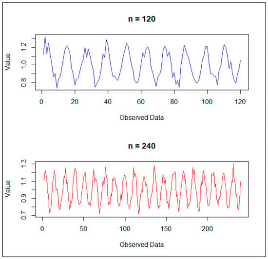
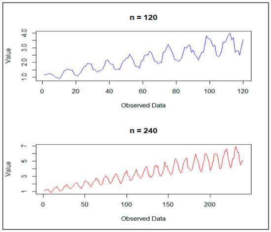
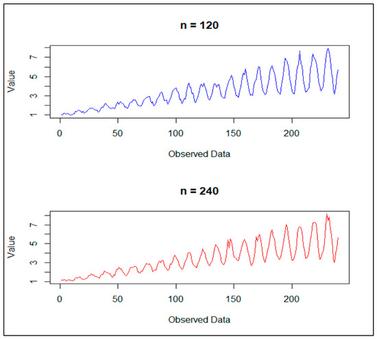
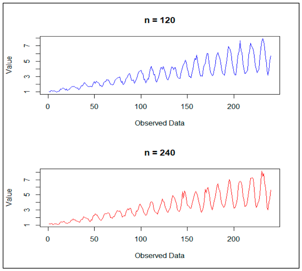
The simulated time series under the no-trend structure are illustrated in Figure 1, the trend-seasonal structure is presented in Figure 2, and the seasonal amplitude structure is shown in Figure 3. In each figure, the blue and red lines correspond to sample sizes of $n=120$ and $n=240$, respectively.

Figure 1. Simulated time series with sample sizes $n\hspace{0.17em}=$ 120 and 240, exhibiting seasonal behavior with a no-trend structure.

Figure 2. Simulated time series with sample sizes $n\hspace{0.17em}=$ 120 and 240, exhibiting seasonal behavior with a trend structure.

Figure 3. Simulated time series with sample sizes $n\hspace{0.17em}=$ 120 and 240, exhibiting seasonal behavior with seasonal amplitude.

To provide a more rigorous evaluation under sparse-data conditions, the missing-data rates were revised to 10%, 30%, and 50%, representing low, moderate, and severe levels of sparsity, respectively. In addition to the conventional seasonal setting, a changing-seasonal-amplitude scenario was introduced to examine forecasting performance when the strength of seasonality evolves over time.

Three imputation methods are implemented prior to model estimation, and seven forecasting accuracy metrics are evaluated using the Mean Absolute Percentage Error (MAPE) and Root Mean Square Error (RMSE).

The MAPE and RMSE are computed as

$$\mathrm{MAPE}\hspace{0.17em}=\hspace{0.17em}{\displaystyle \frac{100}{h}}{\displaystyle \sum _{t=1}^h\left|\frac{y_t-{\widehat{y}}_t}{y_t}\right|}, \mathrm{and} \mathrm{RMSE}\hspace{0.17em}=\hspace{0.17em}\hspace{0.17em}\sqrt{{\displaystyle \frac{{\displaystyle \sum _{t=1}^h{(y_t-{\widehat{y}}_t)}^2}}{h}}}.$$

where $y_t$ denotes the actual observed value, ${\widehat{y}}_t$ represents the corresponding forecasted value, and $h$ denotes the forecast horizon, which is fixed at 12 observations in this study. The MAPE provides a scale-independent measure of prediction accuracy, expressed as a percentage, allowing consistent comparison across different simulation scenarios and sample sizes. The RMSE measures the magnitude of prediction errors in the original scale of the data and assigns greater weight to larger errors through the squared-error formulation.

In this study, the simulation experiment is repeated 1000 times for each configuration to ensure statistical stability and reliability of the results. Consequently, the Average Mean Absolute Percentage Error (AMAPE) and Average Root Mean Squared Error (ARMSE) are computed across all replications and used as the primary performance criterion for identifying the most effective forecasting method. The AMAPE and ARMSE are defined as

$$\mathrm{AMAPE}\hspace{0.17em}=\hspace{0.17em}{\displaystyle \frac{1}{R}}{\displaystyle \sum _{r=1}^R{\mathrm{MAPE}}_r},$$

and

$$\mathrm{ARMSE}\hspace{0.17em}=\hspace{0.17em}{\displaystyle \frac{1}{R}}{\displaystyle \sum _{r=1}^R{\mathrm{RMSE}}_r}.$$

where $R=1000$ denotes the number of simulation replications, and ${\mathrm{MAPE}}_r$ and ${\mathrm{RMSE}}_r$ denote the MAPE and RMSE, respectively, obtained in the $R$th replication. The forecasting approach with the lowest AMAPE is considered the most accurate under the given experimental setting. Similarly, the lowest ARMSE indicates the approach with the smallest overall forecasting error, where lower values represent better predictive performance.

Three imputation methods are implemented prior to model estimation, namely Kalman smoothing (KS) under the Structural Time Series model, seasonal split (SS), and Stineman interpolation (ST).

Following the imputation stage, forecasting analysis is conducted using four specifications of the Generalized Bayesian Structural Time Series framework: GBSTS with Local Level component (GBSTS–LL), GBSTS with Local Linear Trend component (GBSTS–LLT), GBSTS with Local Linear Trend and Seasonal component (GBSTS–LLS), and GBSTS with Local Linear Trend and Trigonometric Seasonal component (GBSTS–LLTS). For comparative benchmarking, four established forecasting methods are also included: the Holt–Winters Seasonal method (HW), the Autoregressive Integrated Moving Average (ARIMA) model, and the Box–Cox transformation, ARMA errors, Trend, and Seasonal components (BATS) model.

Forecasting accuracy is evaluated using the AMAPE and ARMSE to assess both relative percentage errors and the magnitude of forecasting errors across simulation replications. The comparative results are summarized in Table 1, Table 2 and Table 3, providing a detailed assessment of how sample size, sparsity level, seasonal structure, and model specification influence imputation effectiveness and forecasting performance.

Table 1. Simulation results under Kalman smoothing based on the Structural Time Series model, reporting AMAPE and ARMSE for different sample sizes, missing rates, and structural scenarios.

Structural Scenarios	Sample Sizes	Missing Rate	GBSTS-LL	GBSTS-LLT	GBSTS-LLS	GBSTS-LLTS	HW	ARIMA	BATS
Seasonal	n = 120	10%	13.162	12.648	3.897	3.013	4.527	4.951	4.414
			0.148	0.159	0.048	0.038	0.056	0.059	0.054
		30%	13.315	12.909	4.281	3.238	4.965	5.351	4.597
			0.150	0.161	0.052	0.040	0.06	0.063	0.056
		50%	13.283	13.269	5.965	4.010	6.828	6.804	5.337
			0.150	0.165	0.071	0.048	0.080	0.079	0.064
	n = 240	10%	13.351	12.661	4.059	3.166	4.358	5.005	4.366
			0.150	0.155	0.050	0.039	0.053	0.060	0.054
		30%	13.169	12.541	4.326	3.291	4.776	5.299	4.456
			0.148	0.154	0.053	0.041	0.058	0.063	0.055
		50%	13.275	12.952	6.789	4.167	6.449	6.767	4.908
			0.149	0.158	0.079	0.050	0.076	0.078	0.06
Trend and Seasonal	n = 120	10%	12.175	13.044	5.968	7.108	4.521	9.656	4.869
			0.490	0.546	0.223	0.255	0.182	0.372	0.193
		30%	12.282	13.361	6.094	7.225	4.878	10.88	5.389
			0.495	0.558	0.230	0.26	0.195	0.412	0.213
		50%	12.128	13.939	10.285	6.951	6.355	10.891	6.627
			0.484	0.575	0.378	0.253	0.247	0.412	0.258
	n = 240	10%	12.452	13.017	4.745	4.205	4.297	9.076	4.536
			0.839	0.94	0.323	0.282	0.298	0.596	0.315
		30%	12.36	12.986	5.501	4.266	4.696	10.009	4.836
			0.826	0.927	0.368	0.285	0.322	0.645	0.334
		50%	12.436	13.666	14.368	4.657	6.205	11.498	5.83
			0.827	0.974	0.917	0.311	0.418	0.738	0.395
Seasonal Amplitude	n = 120	10%	24.706	23.948	12.072	6.901	6.061	25.597	9.904
			0.902	0.974	0.456	0.241	0.237	0.830	0.411
		30%	24.838	24.16	12.353	6.983	6.993	25.547	10.306
			0.904	0.983	0.470	0.246	0.279	0.826	0.417
		50%	24.800	24.753	15.146	6.827	11.309	16.796	11.246
			0.899	1.000	0.568	0.243	0.431	0.566	0.438
	n = 240	10%	25.743	24.501	11.155	4.029	5.259	22.500	7.277
			1.611	1.708	0.855	0.270	0.359	1.255	0.493
		30%	25.728	24.488	11.491	4.206	5.736	25.338	7.766
			1.596	1.700	0.871	0.280	0.396	1.410	0.517
		50%	25.891	24.991	18.107	4.897	8.267	14.26	9.308
			1.590	1.746	1.245	0.317	0.579	0.836	0.605

Note: Underlined values indicate the lowest AMAPE and RMSE within each configuration.

Table 2. Simulation results under seasonal split interpolation, reporting AMAPE and ARME for different sample sizes, missing rates, and structural scenarios.

Structural Scenarios	Sample Sizes	Missing Rate	GBSTS-LL	GBSTS-LLT	GBSTS-LLS	GBSTS-LLTS	HW	ARIMA	BATS
Seasonal	n = 120	10%	13.164	12.649	3.89	3.017	4.545	5.001	4.42
			0.148	0.158	0.048	0.038	0.056	0.06	0.054
		30%	13.325	12.908	4.331	3.255	5.061	5.535	4.654
			0.15	0.161	0.052	0.041	0.062	0.065	0.057
		50%	13.287	13.273	5.909	4.005	6.832	6.977	5.367
			0.15	0.165	0.071	0.048	0.081	0.081	0.065
	n = 240	10%	13.353	12.664	4.074	3.171	4.378	5.039	4.359
			0.150	0.155	0.05	0.040	0.054	0.06	0.053
		30%	13.325	12.908	4.331	3.255	5.061	5.535	4.654
			0.15	0.161	0.052	0.041	0.062	0.065	0.057
		50%	13.277	12.958	6.764	4.173	6.46	6.794	4.923
			0.149	0.158	0.079	0.050	0.076	0.078	0.06
Trend and Seasonal	n = 120	10%	12.216	13.154	5.924	7.258	4.483	9.832	4.889
			0.496	0.552	0.222	0.260	0.180	0.377	0.194
		30%	12.277	13.438	6.110	7.207	4.852	10.825	5.382
			0.494	0.559	0.232	0.259	0.194	0.410	0.212
		50%	12.109	13.952	10.229	6.903	6.354	11.056	6.609
			0.483	0.576	0.376	0.251	0.247	0.418	0.258
	n = 240	10%	12.462	12.99	4.815	4.168	4.305	9.035	4.573
			0.838	0.936	0.329	0.281	0.300	0.592	0.319
		30%	12.449	12.907	6.242	4.190	4.652	11.228	4.706
			0.827	0.920	0.419	0.279	0.314	0.715	0.319
		50%	12.462	13.611	14.65	4.545	6.154	11.609	5.716
			0.828	0.971	0.93	0.305	0.415	0.743	0.388
Seasonal Amplitude	n = 120	10%	24.712	23.959	12.163	6.864	6.269	24.893	10.076
			0.900	0.972	0.461	0.240	0.244	0.808	0.418
		30%	24.867	24.266	12.874	6.797	8.000	27.636	11.016
			0.899	0.978	0.497	0.241	0.311	0.887	0.436
		50%	24.874	25.271	17.863	6.623	13.981	21.190	12.879
			0.890	1.004	0.669	0.238	0.518	0.706	0.488
	n = 240	10%	25.775	24.518	11.389	3.987	5.451	20.855	7.516
			1.609	1.705	0.873	0.268	0.369	1.167	0.509
		30%	25.86	24.587	12.969	4.115	6.832	29.646	8.672
			1.587	1.694	0.979	0.280	0.456	1.619	0.566
		50%	26.056	25.379	23.412	5.065	10.661	21.976	11.671
			1.571	1.752	1.545	0.325	0.726	1.233	0.735

Note: Underlined values indicate the lowest AMAPE and RMSE within each configuration.

Table 3. Simulation results under Stine interpolation, reporting AMAPE and ARMSE for different sample sizes, missing rates, and structural scenarios.

Structural Scenarios	Sample Sizes	Missing Rate	GBSTS-LL	GBSTS-LLT	GBSTS-LLS	GBSTS-LLTS	HW	ARIMA	BATS
Seasonal	n = 120	10%	13.162	12.652	3.896	3.019	4.562	4.996	4.427
			0.148	0.159	0.048	0.038	0.056	0.060	0.055
		30%	13.318	12.909	4.291	3.269	5.054	5.472	4.608
			0.150	0.161	0.052	0.041	0.062	0.064	0.056
		50%	13.269	13.286	5.711	4.059	7.055	6.964	5.266
			0.150	0.166	0.068	0.049	0.083	0.081	0.064
	n = 240	10%	13.352	12.664	4.068	3.174	4.368	5.031	4.367
			0.150	0.155	0.050	0.040	0.054	0.060	0.054
		30%	13.198	12.688	4.356	3.353	4.815	5.428	4.484
			0.148	0.154	0.053	0.042	0.058	0.064	0.055
		50%	13.260	12.941	6.469	4.208	6.676	6.869	4.832
			0.149	0.158	0.075	0.051	0.079	0.079	0.059
Trend and Seasonal	n = 120	10%	12.056	13.005	5.561	7.144	4.306	9.847	4.731
			0.487	0.543	0.211	0.256	0.173	0.370	0.189
		30%	12.306	13.39	5.981	6.756	4.888	11.604	5.384
			0.496	0.555	0.229	0.243	0.193	0.439	0.21
		50%	12.316	14.024	9.483	7.049	6.694	9.952	6.714
			0.493	0.578	0.351	0.257	0.260	0.384	0.264
	n = 240	10%	12.53	13.073	4.796	4.319	4.337	8.262	4.572
			0.846	0.939	0.326	0.289	0.300	0.548	0.319
		30%	12.579	13.339	5.553	4.495	4.758	10.429	4.956
			0.844	0.953	0.38	0.301	0.329	0.671	0.343
		50%	12.616	13.676	13.53	4.668	6.214	10.471	5.488
			0.843	0.979	0.861	0.312	0.418	0.678	0.376
Seasonal Amplitude	n = 120	10%	24.71	23.96	12.137	6.888	6.202	25.538	9.928
			0.901	0.973	0.459	0.241	0.242	0.827	0.410
		30%	24.725	24.164	12.685	6.998	7.796	23.473	10.447
			0.898	0.976	0.481	0.246	0.305	0.766	0.419
		50%	24.862	25.347	17.628	6.818	13.538	16.249	12.531
			0.895	1.007	0.651	0.243	0.500	0.563	0.476
	n = 240	10%	25.695	24.48	11.272	4.158	5.328	22.394	7.255
			1.613	1.711	0.86	0.276	0.364	1.253	0.494
		30%	25.839	24.532	12.561	4.228	6.346	26.224	8.444
			1.588	1.699	0.954	0.281	0.429	1.449	0.555
		50%	26.159	25.473	21.197	5.377	10.89	17.651	11.441
			1.589	1.77	1.434	0.340	0.738	1.028	0.73

Note: Underlined values indicate the lowest AMAPE and RMSE within each configuration.

Table 1 presents the forecasting performance under Kalman smoothing across different sample sizes, missing rates, and structural scenarios. Overall, GBSTS–LLTS achieved the lowest AMAPE values in the Seasonal and Seasonal Amplitude scenarios, demonstrating its ability to capture seasonal dynamics. In contrast, Holt–Winters (HW) generally produced the lowest AMAPE in the Trend and Seasonal scenarios. Forecasting errors tended to increase as the missing rate increased, particularly under the more complex Seasonal Amplitude structure. The ARMSE results generally supported the AMAPE patterns, although some differences among methods were observed.

Table 2 presents the forecasting performance under seasonal split interpolation for different sample sizes, missing rates, and structural scenarios. The GBSTS–LLTS consistently achieved the lowest AMAPE values in the Seasonal and Seasonal Amplitude scenarios, indicating strong performance in modeling seasonal structures. For the Trend and Seasonal scenarios, HW generally yielded the lowest AMAPE, particularly for n = 120, while GBSTS–LLTS became competitive for n = 240 at higher missing rates. Forecasting errors generally increased with increasing missing rates, with a more pronounced effect under the Seasonal Amplitude scenario. The ARMSE results broadly complemented the AMAPE findings, although the best-performing method differed in some configurations.

Table 3 presents the forecasting performance under Stine interpolation across different sample sizes, missing rates, and structural scenarios. The GBSTS–LLTS achieved the lowest AMAPE values in the Seasonal and Seasonal Amplitude scenarios, indicating its effectiveness in capturing seasonal patterns. In contrast, Holt–Winters (HW) provided the lowest AMAPE in the Trend and Seasonal scenarios. Forecasting errors generally increased as the missing rate increased, reflecting the adverse effect of data sparsity. The ARMSE results broadly supported the AMAPE findings, although some differences among methods were observed. These results suggest that forecasting performance depends strongly on the underlying structural characteristics of the time series.

To complement the forecasting accuracy measures reported in Table 1, Table 2 and Table 3, the Diebold–Mariano (DM) [50] test was employed to formally assess whether the predictive performance of the proposed GBSTS–LLTS model differed significantly from that of the benchmark forecasting methods. The test was conducted by comparing the forecast loss of GBSTS–LLTS with those of Holt–Winters (HW), ARIMA, and BATS under each structural scenario, sample size, missing rate, and imputation strategy.

The loss differential between GBSTS–LLTS and a competing method was defined as

$$d_t\hspace{0.17em}=\hspace{0.17em}L(e_{G,t})-L(e_{B,t})$$

where $e_{G,t}$ and $e_{B,t}$ denote the forecast errors from GBSTS–LLTS and the benchmark method, respectively, and L(⋅) denotes the loss function. The null and alternative hypotheses of the DM test are

$$H_0\hspace{0.17em}\hspace{0.17em}=\hspace{0.17em}E(d_t)=0,\hspace{0.17em}\hspace{0.17em}\hspace{0.17em}\hspace{0.17em}\hspace{0.17em}\hspace{0.17em}\hspace{0.17em}\hspace{0.17em}\hspace{0.17em}\hspace{0.17em}\hspace{0.17em}\hspace{0.17em}{H}_1\hspace{0.17em}=\hspace{0.17em}E(d_t)<0,$$

indicating equal predictive accuracy between the two forecasting methods. A heteroskedasticity- and autocorrelation-consistent (HAC) variance estimator was used to account for possible serial dependence in the loss differential. A statistically significant negative DM statistic indicates that GBSTS–LLTS yields a significantly lower forecast loss than the corresponding benchmark method. The significance level was set at 5% throughout the analysis.

The DM test results therefore provide formal statistical evidence complementing the AMAPE and ARMSE comparisons reported in Table 1, Table 2 and Table 3 and help determine whether the observed differences in forecasting performance are statistically significant rather than merely numerical. Pairwise DM tests were subsequently conducted between the proposed GBSTS–LLTS model and each benchmark forecasting method under the different imputation strategies and structural scenarios. The results of these pairwise comparisons are summarized in Table 4.

Table 4. Summary of pairwise Diebold–Mariano test results comparing GBSTS–LLTS with benchmark forecasting methods across structural scenarios.

Scenario	GBSTS–LLTS vs. HW	GBSTS–LLTS vs. ARIMA	GBSTS–LLTS vs. BATS
Seasonal	Significant improvement	Significant improvement	Significant improvement
Trend and Seasonal	Mostly not significant (HW superior)	Significant in some cases	Mostly significant
Seasonal Amplitude	Mixed	Mostly significant	Mostly significant

Table 4 summarizes the pairwise Diebold–Mariano test results comparing GBSTS–LLTS with HW, ARIMA, and BATS across the three structural scenarios. Under the Seasonal scenario, GBSTS–LLTS showed statistically significant improvements over all benchmark methods, confirming its strong ability to capture seasonal patterns. For the Trend and Seasonal scenario, GBSTS–LLTS generally did not significantly outperform HW, and HW was superior in several configurations, whereas significant improvements were observed in some comparisons with ARIMA and in most comparisons with BATS. For the Seasonal Amplitude scenario, the comparison with HW produced mixed results, while GBSTS–LLTS significantly outperformed ARIMA and BATS in most configurations.

These statistical findings are consistent with the forecasting performance summarized in Table 5, further demonstrating that the relative advantage of each forecasting method depends on the underlying structural characteristics of the time series.

Table 5. Summary of the best-performing forecasting methods and the corresponding lowest AMAPE values under each imputation strategy, sample size, missing rate, and structural scenario.

Structural Scenarios	Sample Sizes	Missing Rate	KS	SS	ST
Seasonal	n = 120	10%	GBSTS-LLTS	GBSTS-LLTS	GBSTS-LLTS
			3.013	3.017	3.019
		30%	GBSTS-LLTS	GBSTS-LLTS	GBSTS-LLTS
			3.328	3.255	3.269
		50%	GBSTS-LLTS	GBSTS-LLTS	GBSTS-LLTS
			4.010	4.005	4.059
	n = 240	10%	GBSTS-LLTS	GBSTS-LLTS	GBSTS-LLTS
			3.166	3.171	3.174
		30%	GBSTS-LLTS	GBSTS-LLTS	GBSTS-LLTS
			3.291	3.255	3.535
		50%	GBSTS-LLTS	GBSTS-LLTS	GBSTS-LLTS
			4.167	4.173	4.208
Trend and Seasonal	n = 120	10%	HW	HW	HW
			4.521	4.483	4.306
		30%	HW	HW	HW
			4.878	4.852	4.888
		50%	HW	HW	HW
			6.355	6.354	6.694
	n = 240	10%	GBSTS-LLTS	GBSTS-LLTS	GBSTS-LLTS
			4.205	4.168	4.319
		30%	GBSTS-LLTS	GBSTS-LLTS	GBSTS-LLTS
			4.266	4.190	4.495
		50%	GBSTS-LLTS	GBSTS-LLTS	GBSTS-LLTS
			4.657	4.545	4.668
Seasonal Amplitude	n = 120	10%	HW	HW	HW
			6.061	6.269	6.202
		30%	GBSTS-LLTS	GBSTS-LLTS	GBSTS-LLTS
			6.983	6.797	6.998
		50%	GBSTS-LLTS	GBSTS-LLTS	GBSTS-LLTS
			6.827	6.623	6.818
	n = 240	10%	GBSTS-LLTS	GBSTS-LLTS	GBSTS-LLTS
			4.029	3.987	4.158
		30%	GBSTS-LLTS	GBSTS-LLTS	GBSTS-LLTS
			4.206	4.115	4.228
		50%	GBSTS-LLTS	GBSTS-LLTS	GBSTS-LLTS
			4.897	5.065	5.377

Note: Underlined values indicate the lowest AMAPE within each configuration.

Table 5 summarizes the results obtained from Table 1, Table 2 and Table 3 by identifying the best-performing forecasting method and the corresponding lowest AMAPE value for each imputation strategy, sample size, missing rate, and structural scenario. Overall, GBSTS–LLTS was the dominant method in the Seasonal scenario across all imputation strategies (KS, SS, and ST), while HW performed better in several Trend and Seasonal configurations. For the Seasonal Amplitude scenario, HW was preferable at a low missing rate for n = 120, whereas GBSTS–LLTS generally provided the lowest AMAPE as the missing rate increased and for n = 240. Across the three imputation strategies, seasonal split interpolation (SS) frequently produced the lowest AMAPE, although Kalman smoothing (KS) was superior in several configurations. These results demonstrate that the optimal forecasting–imputation combination depends on the structural scenario, sample size, and degree of missingness.

In general, Kalman smoothing (KS) and Seasonal Split (SS) interpolation slightly outperform the other imputation methods in several model–dataset combinations. However, the differences in AMAPE are generally small, indicating that the leading imputation methods perform comparably under specific conditions rather than demonstrating a substantial advantage of one method over the others.

5. Application in Real Data Set

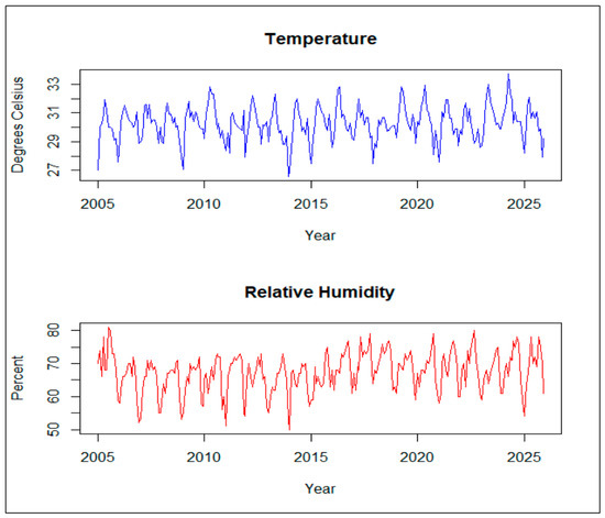
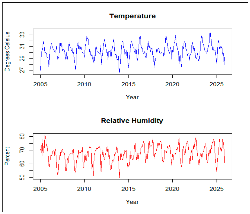
To demonstrate the practical applicability of the proposed approach, a real-world dataset consisting of monthly average temperature and relative humidity observations is analyzed. The data were collected from the Khlong Toei meteorological station in Bangkok, Thailand, covering the period from January 2005 to December 2025, from the Thai Meteorological Department (TMD) (https://www.tmd.go.th/, accessed on 9 March 2026). These variables are widely used as indicators of local climate variability and exhibit clear seasonal patterns. The time series plots of the monthly average temperature and relative humidity are shown in Figure 4, where the blue and red lines represent the monthly average temperature and relative humidity, respectively, and the corresponding descriptive statistics are summarized in Table 6.

Figure 4. Time series plots of monthly average temperature (°C) and relative humidity (%) recorded at the Khlong Toei meteorological station in Bangkok, Thailand, from January 2005 to December 2025.

Table 6. Descriptive statistics for monthly average temperature (°C) and relative humidity (%) at the Khlong Toei meteorological station in Bangkok, Thailand, from January 2005 to December 2025.

Meteorological Variables	Mean	Median	SD	Min	Max	CV	Trend	Seasonal
Temperature	30.280	30.3	1.181	26.6	33.7	3.900	0.332	0.715
Relative Humidity	67.353	68.0	6.023	50	81	8.942	0.126	0.678

Figure 4 illustrates the monthly time series of temperature and relative humidity at the Khlong Toei station, where both variables exhibit clear seasonal fluctuations throughout the observation period. This visual pattern is consistent with the descriptive statistics reported in Table 6. Specifically, the seasonal indices are relatively high for both variables (0.714 for temperature and 0.678 for relative humidity), indicating strong seasonality. The trend values (0.332 and 0.126) indicate moderate long-term variation. In addition, the summary statistics show that the mean temperature is approximately 30.28 °C with relatively low variability (SD = 1.181), while relative humidity has a mean of 67.35% and slightly higher variability (SD = 3.023). These statistical characteristics align with the seasonal patterns observed in Figure 4, supporting the dataset’s suitability for evaluating forecasting models under seasonal time-series conditions.

To evaluate the forecasting performance under sparse observations, three imputation methods are applied prior to model estimation. The original dataset contains no missing values; therefore, missing observations are artificially generated by randomly removing 10%, 30%, and 50% of the data points to simulate sparsity, and this process is repeated 1000 times. The forecasting results for the temperature series are summarized in Table 7, while the corresponding results for the relative humidity series are presented in Table 8. The values reported in both tables represent the Average Mean Absolute Percentage Error (AMAPE) and Average Root Mean Squared Error (ARMSE), calculated based on a fixed forecast horizon of 12 observations.

Table 7. Average Mean Absolute Percentage Error (AMAPE) and Average Root Mean Squared Error (ARMSE) in forecasting models for the temperature series under different imputation methods and missing rates.

Imputation Methods	Missing Rate	GBSTS-LL	GBSTS-LLT	GBSTS-LLS	GBSTS-LLTS	HW	ARIMA	BATS
KS	10%	3.479	3.669	2.892	2.189	2.700	3.101	2.196
		1.303	1.413	0.954	0.754	1.093	1.140	0.951
	30%	3.472	3.646	2.988	2.168	2.437	3.156	2.189
		1.301	1.402	0.993	0.749	0.991	1.154	0.913
	50%	3.456	3.412	3.782	2.061	2.461	3.298	2.289
		1.296	1.299	1.275	0.713	0.965	1.198	0.905
SS	10%	3.48	3.668	2.88	2.19	2.692	3.093	2.197
		1.302	1.413	0.950	0.754	1.090	1.138	0.951
	30%	3.475	3.64	2.915	2.159	2.401	3.120	2.175
		1.300	1.399	0.965	0.745	0.975	1.145	0.908
	50%	3.467	3.422	3.512	2.062	2.387	3.208	2.187
		1.299	1.306	1.185	0.725	0.908	1.173	0.85
ST	10%	3.480	3.665	2.891	2.190	2.711	3.086	2.196
		1.301	1.412	0.954	0.755	1.093	1.136	0.949
	30%	3.475	3.617	2.895	2.147	2.458	3.083	2.217
		1.298	1.391	0.959	0.741	0.992	1.135	0.916
	50%	3.474	3.453	3.299	2.072	2.400	3.137	2.155
		1.302	1.322	1.111	0.734	0.902	1.154	0.841

Note: Underlined values indicate the lowest AMAPE and RMSE within each configuration.

Table 8. Average Mean Absolute Percentage Error (AMAPE) and Average Root Mean Squared Error (RMSE) in forecasting models for the relative humidity series under different imputation methods and missing rates.

Imputation Methods	Missing Rate	GBSTS-LL	GBSTS-LLT	GBSTS-LLS	GBSTS-LLTS	HW	ARIMA	BATS
KS	10%	8.245	8.133	5.380	2.973	4.677	9.615	4.576
		6.971	6.899	4.284	2.360	4.080	7.741	3.934
	30%	8.252	8.219	5.678	3.145	5.174	9.574	4.871
		6.961	6.935	4.542	2.442	4.48	7.775	4.177
	50%	8.287	8.553	6.242	3.489	6.238	8.506	5.677
		6.969	7.157	5.059	2.734	5.273	7.038	4.804
SS	10%	8.248	8.121	5.403	2.977	4.645	11.591	4.596
		6.972	6.889	4.296	2.359	4.067	9.293	3.942
	30%	8.227	8.222	5.595	3.141	5.084	9.523	4.646
		6.966	6.942	4.478	2.402	4.456	7.667	4.040
	50%	8.32	8.882	6.393	4.003	7.920	6.920	5.024
		7.011	7.413	5.054	2.994	6.554	5.829	4.376
ST	10%	8.250	8.116	5.411	2.963	4.651	11.675	4.607
		6.973	6.888	4.300	2.351	4.077	9.325	3.949
	30%	8.251	8.226	5.552	3.140	5.103	9.419	4.619
		6.970	6.943	4.429	2.395	4.461	7.62	4.016
	50%	8.319	8.562	6.198	3.721	7.631	7.715	4.874
		7.000	7.175	4.913	2.787	6.297	6.457	4.258

Note: Underlined values indicate the lowest AMAPE and RMSE within each configuration.

Table 7 and Table 8 present the forecasting performance for the temperature and relative humidity series, respectively, under different imputation methods and missing rates. Overall, GBSTS–LLTS consistently achieved the lowest AMAPE and RMSE values across all imputation methods and missing rates for both meteorological variables, demonstrating its robust forecasting performance. For the temperature series, the differences among KS, SS, and ST were relatively small, with GBSTS–LLTS maintaining its superior performance as the missing rate increased. A similar pattern was observed for relative humidity, although forecasting errors were generally larger than those for temperature. Among the benchmark methods, HW and BATS generally performed better than ARIMA, but they were consistently outperformed by GBSTS–LLTS. These findings indicate that GBSTS–LLTS provides stable and accurate forecasts across different levels of missingness and imputation strategies in both temperature and relative humidity series.

The original meteorological datasets contained no missing observations. To provide a controlled evaluation of forecasting performance under varying levels of sparsity, missing observations were artificially introduced at 10%, 30%, and 50% rates via a random deletion mechanism. Therefore, the resulting incomplete datasets represent controlled experimental missingness rather than naturally occurring missing-data processes. This design facilitates consistent comparisons across forecasting and imputation methods, but it does not capture all mechanisms through which missing observations may arise in real-world applications.

6. Discussion

The results obtained from both the simulation study and the empirical analysis provide important insights into forecasting seasonal time series with sparse observations. The findings indicate that forecasting performance depends strongly on the underlying temporal structure, sample size, and degree of missingness. Overall, GBSTS–LLTS demonstrated strong performance for seasonal and changing-seasonal-amplitude processes, suggesting that combining a local linear trend with trigonometric seasonal components provides sufficient flexibility to capture smooth and evolving periodic patterns. This result is consistent with the structural time-series literature, which emphasizes the benefits of explicitly modeling latent trend and seasonal components [4,5,6,29], as well as previous studies highlighting the importance of flexible representations for complex seasonal patterns [13,14,16].

However, the proposed model did not uniformly dominate the competing methods. Holt–Winters was particularly competitive for the Trend and Seasonal scenario with smaller samples, whereas GBSTS–LLTS became more favorable as the sample size increased. A similar pattern occurred under changing seasonal amplitude, where Holt–Winters performed well under low missingness with smaller samples, while GBSTS–LLTS generally showed greater advantages under more complex conditions. These findings emphasize that increased model flexibility does not necessarily guarantee superior forecasting accuracy and that model performance depends on the compatibility between the model structure and the underlying data-generating process. This observation is consistent with established findings on exponential smoothing and structural time-series forecasting [5,30,37,38,39,40].

The results also demonstrate the importance of the interaction between missing-data imputation and forecasting. No imputation strategy uniformly dominated across all experimental settings, although approaches that preserved temporal and seasonal information generally produced competitive forecasts. Kalman-based methods provide a theoretically coherent state-space mechanism for reconstructing missing observations [5,6,45,46,47], whereas interpolation methods can effectively preserve smooth local and seasonal structures [31,32,48,49]. Therefore, the choice of imputation method should be considered jointly with the subsequent forecasting model rather than as an entirely independent preprocessing step.

The empirical analysis of temperature and relative humidity further supports the practical applicability of the proposed framework. GBSTS–LLTS consistently provided strong forecasting accuracy for both meteorological variables across different missing rates and imputation strategies. These results suggest that its stochastic trend and trigonometric seasonal representation are well suited to meteorological series characterized by pronounced periodic behavior. Similar applications have demonstrated the usefulness of structural time-series and flexible seasonal models for environmental and meteorological data [2,44].

Finally, comparisons with ARIMA, BATS, and Holt–Winters show that established forecasting approaches remain competitive under particular temporal structures [14,30,37,40,41,42,43,44]. Thus, the contribution of GBSTS–LLTS should not be interpreted as universal superiority over existing methods. Rather, the results demonstrate its value as a flexible Bayesian structural forecasting framework, particularly when seasonal dynamics are prominent or evolve over time. This balanced interpretation is consistent with the broader forecasting literature, which recognizes that forecasting performance is inherently dependent on the characteristics of the data and model specification [14,30].

The findings of this study should be interpreted within the scope of the experimental design. Although the proposed framework was evaluated using both simulated and empirical meteorological time series, the empirical datasets were originally complete, and missing observations were artificially introduced via a controlled random mechanism. Consequently, the results demonstrate the performance of the proposed framework under controlled sparse-data conditions but do not establish equivalent performance for naturally incomplete datasets. In particular, economic and business time series may exhibit non-random missingness, structural breaks, intermittent demand, irregular observation intervals, and abrupt changes in trend or seasonality that are not fully represented in the present experiments. Therefore, the generalizability of the current findings to such settings requires further empirical investigation.

Future research should therefore evaluate the proposed GBSTS framework under more complex data-generating processes, including structural breaks and abrupt changes in temporal dynamics, as well as a broader range of additive and multiplicative seasonal patterns. Such extensions would provide a more comprehensive assessment of the framework’s robustness under complex and dynamically evolving seasonal structures.

7. Conclusions

This study proposes a generalized Bayesian structural time series (GBSTS) framework for forecasting seasonal time series with sparse observations. The proposed approach extends the conventional BSTS formulation by integrating alternative structural components, including local level, local linear trend, and different seasonal representations, within a unified Bayesian state-space framework. We evaluated its forecasting performance using Monte Carlo simulations across different sample sizes, missing rates, and temporal structures, along with an empirical analysis of temperature and relative humidity data. The comparison was further extended to established forecasting methods, including Holt, Holt–Winters, ARIMA, and BATS.

The simulation results show that the Generalized Bayesian Structural Time Series with Local Linear Trend and Trigonometric Seasonal Component (GBSTS–LLTS) generally performed best under seasonal and changing-seasonal-amplitude scenarios, whereas Holt–Winters remained competitive and performed better in several trend and seasonal settings, particularly for smaller samples. No single imputation method consistently dominated across all conditions. The empirical analysis further showed that GBSTS–LLTS provided the lowest forecasting errors for both temperature and relative humidity across the examined missing rates and imputation strategies. The Diebold–Mariano tests with HAC variance estimation also provided statistical support for the forecasting improvements observed in several configurations. In addition, while the present study employs pairwise Diebold–Mariano tests to assess predictive accuracy, future research could consider multiple-model forecast comparison procedures, such as the Superior Predictive Ability (SPA) test [51], particularly when several competing forecasting methods are evaluated simultaneously.

A limitation of the present study is that missing observations were generated randomly at predetermined rates, whereas consecutive or blockwise missing-data patterns were not explicitly considered. In practical time-series applications, observations may be unavailable for consecutive periods due to sensor failures, data transmission interruptions, or other systematic disruptions. The performance of imputation and forecasting methods under such conditions may depend on the length, location, and frequency of the missing blocks. Future research should therefore extend the proposed GBSTS framework to investigate blockwise missingness of varying lengths and compare its robustness with that observed under randomly distributed missing-data mechanisms. Further investigation should also consider more complex time-series structures, including structural breaks and a broader range of additive and multiplicative seasonal patterns.

References

- Gianacas, C.; Liu, B.; Kirk, M.; Di Tanna, G.L.; Belcher, J.; Blogg, S.; Muscatello, D.J. Bayesian Structural Time Series, an Alternative to Interrupted Time Series in the Right Circumstances. J. Clin. Epidemiol. 2023, 163, 102–110. [Google Scholar] [CrossRef] [Scilit] [PubMed]
- Liang, W.; Li, Y.; Liu, X.; Dai, Q.; Feng, Y. AI-based Bayesian structural time series modeling for assessing PM2.5 air quality improvements during the Beijing 2022 Winter Olympics. Atmos. Environ. 2025, 358, 121328. [Google Scholar] [CrossRef] [Scilit]
- Xie, L. The analysis and forecasting COVID-19 cases in the United States using Bayesian structural time series models. Biostat. Epidemiol. 2022, 6, 1–15. [Google Scholar] [CrossRef] [Scilit]
- West, M.; Harrison, J. Bayesian Forecasting and Dynamic Models, 2nd ed.; Springer: New York, NY, USA, 1997. [Google Scholar]
- Harvey, A.C. Forecasting, Structural Time Series Models and the Kalman Filter; Cambridge University Press: Cambridge, UK, 1989. [Google Scholar]
- Durbin, J.; Koopman, S.J. Time Series Analysis by State Space Methods, 2nd ed.; Oxford University Press: Oxford, UK, 2012. [Google Scholar]
- Scott, S.L.; Varian, H.R. Predicting the Present with Bayesian Structural Time Series. Int. J. Math. Model. Numer. Optim. 2014, 5, 4–23. [Google Scholar] [CrossRef] [Scilit]
- Brodersen, K.H.; Gallusser, F.; Koehler, J.; Remy, N.; Scott, S.L. Inferring Causal Impact Using Bayesian Structural Time-Series Models. Ann. Appl. Stat. 2015, 9, 247–274. [Google Scholar] [CrossRef] [Scilit]
- Jun, S. Bayesian Structural Time Series and Regression Modeling for Sustainable Technology Management. Sustainability 2019, 11, 4945. [Google Scholar] [CrossRef] [Scilit]
- Almarashi, A.M.; Khan, K. Bayesian Structural Time Series. Nanosci. Nanotechnol. Lett. 2020, 12, 54–61. [Google Scholar] [CrossRef] [Scilit]
- Hamza, M.; Mohammad, A. A Comparison of the Bayesian Structural Time Series Technique with the ARIMA Model for Forecasting. Migr. Lett. 2024, 21, 528–538. [Google Scholar]
- Rizal, R.; Zuliana, S. Forecasting Using SARIMA and Bayesian Structural Time Series Method for Seasonal Data. Proc. Int. Conf. Data Sci. Off. Stat. 2023, 2023, 382–391. [Google Scholar] [CrossRef] [Scilit]
- Taylor, J.W. Triple Seasonal Methods for Short-Term Electricity Demand Forecasting. Eur. J. Oper. Res. 2010, 204, 139–152. [Google Scholar] [CrossRef] [Scilit]
- De Livera, A.M.; Hyndman, R.J.; Snyder, R.D. Forecasting Time Series with Complex Seasonal Patterns Using Exponential Smoothing. J. Am. Stat. Assoc. 2011, 106, 1513–1527. [Google Scholar] [CrossRef] [Scilit]
- Bandara, K.; Bergmeir, C.; Smyl, S. Forecasting Across Time Series Databases Using Recurrent Neural Networks on Groups of Similar Series: A Clustering Approach. Expert Syst. Appl. 2020, 140, 112896. [Google Scholar] [CrossRef] [Scilit]
- Gould, P.G.; Koehler, A.B.; Snyder, R.D.; Ord, J.K.; Vahid-Araghi, F. Forecasting Time-Series with Multiple Seasonal Patterns. Eur. J. Oper. Res. 2008, 191, 207–222. [Google Scholar] [CrossRef] [Scilit]
- Taieb, S.B.; Hyndman, R.J. A Gradient Boosting Approach to the Kaggle Load Forecasting Competition. Int. J. Forecast. 2014, 30, 382–394. [Google Scholar] [CrossRef] [Scilit]
- Bergmeir, C.; Hyndman, R.J.; Benítez, J.M. Bagging Exponential Smoothing Methods Using STL Decomposition and Box–Cox Transformation. Int. J. Forecast. 2016, 32, 303–312. [Google Scholar] [CrossRef] [Scilit]
- Andrews, A.; Kimpton, S. Econometric Forecasting of Tourist Arrivals Using Bayesian Structural Time-Series. Econ. Pap. 2023, 42, 200–211. [Google Scholar] [CrossRef] [Scilit]
- Petris, G.; Petrone, S.; Campagnoli, P. Dynamic Linear Models with R; Springer: New York, NY, USA, 2009. [Google Scholar]
- Carlin, B.P.; Polson, N.G.; Stoffer, D.S. A Monte Carlo Approach to Nonlinear and Non-Gaussian State-Space Models. J. Am. Stat. Assoc. 1992, 87, 493–500. [Google Scholar] [CrossRef]
- Frühwirth-Schnatter, S. Finite Mixture and Markov Switching Models; Springer: New York, NY, USA, 2006. [Google Scholar]
- Gelman, A.; Carlin, J.B.; Stern, H.S.; Dunson, D.B.; Vehtari, A.; Rubin, D.B. Bayesian Data Analysis, 3rd ed.; CRC Press: Boca Raton, FL, USA, 2013. [Google Scholar]
- Du, W.; Côté, D.; Liu, Y. SAITS: Self-attention-based imputation for time series. Expert Syst. Appl. 2023, 219, 119619. [Google Scholar] [CrossRef] [Scilit]
- Jin, K.; Blanco-Encomienda, F.J. Seasonal Decomposition-Enhanced Deep Learning Architecture for Probabilistic Forecasting. J. Forecast. 2025, 45, 880–891. [Google Scholar] [CrossRef] [Scilit]
- Lu, G.; Ou, Y.; Wang, Z.; Qu, Y.; Xia, Y.; Tang, D.; Kotenko, I.; Li, W. A Survey of Deep Learning for Time Series Forecasting: Theories, Datasets, and State-of-the-Art Techniques. Comput. Mater. Contin. 2025, 85, 2403–2441. [Google Scholar] [CrossRef] [Scilit]
- Meda-Campaña, J.A.; Velázquez-Sánchez, R.D.; García-Hernández, J.C.; Torres-Cedillo, S.; Tapia-Herrera, R. Online Sparse Identification of Nonlinear State-Space Equations via RLS. Int. J. Control Autom. Syst. 2025, 23, 2232–2246. [Google Scholar] [CrossRef] [Scilit]
- Qu, K.; Xue, S.; Zheng, X.; Yan, D.; Cao, H. Learning dynamic inter-farm dependencies for wind power forecasting via adaptive sparse graph attention network. Renew. Energy 2026, 258, 124969. [Google Scholar] [CrossRef] [Scilit]
- Prado, R.; West, M. Time Series: Modeling, Computation, and Inference; Chapman & Hall/CRC: Boca Raton, FL, USA, 2010. [Google Scholar]
- Hyndman, R.J.; Athanasopoulos, G. Forecasting: Principles and Practice, 3rd ed.; OTexts: Melbourne, Australia, 2021. [Google Scholar]
- Soper, D.S. High-Speed Scientific Computing Using Adaptive Spline Interpolation. Big Data Cogn. Comput. 2025, 9, 308. [Google Scholar] [CrossRef] [Scilit]
- Stineman, R.W. A Consistently Well-Behaved Method of Interpolation. Creat. Comput. 1980, 6, 54–57. [Google Scholar]
- Andrieu, C.; De Freitas, N.; Doucet, A.; Jordan, M.I. An Introduction to MCMC for Machine Learning. Mach. Learn. 2003, 50, 5–43. [Google Scholar] [CrossRef] [Scilit]
- Shephard, N.; Pitt, M.K. Likelihood Analysis of Non-Gaussian Measurement Time Series. Biometrika 1997, 84, 653–667. [Google Scholar] [CrossRef] [Scilit]
- Carter, C.K.; Kohn, R. On Gibbs Sampling for State Space Models. Biometrika 1994, 81, 541–553. [Google Scholar] [CrossRef] [Scilit] [PubMed]
- Chib, S.; Greenberg, E. Understanding the Metropolis–Hastings Algorithm. Am. Stat. 1995, 49, 327–335. [Google Scholar] [CrossRef] [Scilit]
- Holt, C.C. Forecasting Seasonals and Trends by Exponentially Weighted Moving Averages. Int. J. Forecast. 2004, 20, 5–10. [Google Scholar] [CrossRef] [Scilit]
- Gardner, E.S. Exponential Smoothing: The State of the Art. J. Forecast. 1985, 4, 1–28. [Google Scholar] [CrossRef] [Scilit]
- Gardner, E.S. Exponential Smoothing: The State of the Art—Part II. Int. J. Forecast. 2006, 22, 637–666. [Google Scholar] [CrossRef] [Scilit]
- Winters, P.R. Forecasting Sales by Exponentially Weighted Moving Averages. Manag. Sci. 1960, 6, 324–342. [Google Scholar] [CrossRef] [Scilit]
- Welagedara, W.A.D.M.; Haile, M.G.; Olive, D.J. ARIMA Model Selection and Prediction Intervals. Axioms 2026, 15, 228. [Google Scholar] [CrossRef] [Scilit]
- da Veiga, C.P.; da Veiga, C.R.P.; Girotto, F.M.; Marconatto, D.A.B.; Su, Z. Implementa-tion of the ARIMA model for prediction of economic variables: Evidence from the health sector in Brazil. Humanit. Soc. Sci. Commun. 2024, 11, 1068. [Google Scholar] [CrossRef] [Scilit]
- Chudo, S.B.; Terdik, G. Modeling and Forecasting Time-Series Data with Multiple Seasonal Periods Using Periodograms. Econometrics 2025, 13, 14. [Google Scholar] [CrossRef] [Scilit]
- Ray, M.; Sahoo, K.C.; Abotaleb, M.; Ray, S.; Sahu, P.K.; Mishra, P.; Al Khatib, A.M.G.; Das, S.S.; Jain, V.; Balloo, R. Modeling and forecasting metrological factors using BATS and TBATS models for Keonjhar district of Orissa. MAUSAM 2022, 73, 555–564. [Google Scholar] [CrossRef] [Scilit]
- Koopman, S.J.; Harvey, A.C. Computing Observation Weights for Signal Extraction and Filtering. J. Econ. 2003, 112, 67–88. [Google Scholar]
- Durbin, J.; Koopman, S.J. A Simple and Efficient Simulation Smoother for State Space Time Series Analysis. Biometrika 2002, 89, 603–616. [Google Scholar] [CrossRef] [Scilit]
- Moritz, S.; Bartz-Beielstein, T. imputeTS: Time Series Missing Value Imputation in R. R J. 2017, 9, 207–218. [Google Scholar] [CrossRef] [Scilit]
- Fritsch, F.N.; Carlson, R.E. Monotone Piecewise Cubic Interpolation. SIAM J. Numer. Anal. 1980, 17, 238–246. [Google Scholar] [CrossRef] [Scilit]
- Fritsch, F.N.; Butland, J. A Method for Constructing Local Monotone Piecewise Cubic Interpolants. SIAM J. Sci. Stat. Comput. 1984, 5, 300–304. [Google Scholar] [CrossRef] [Scilit]
- Cuaresma, J.C.; Hlouskova, J.; Kossmeier, S.; Obersteiner, M. Forecasting electricity spot-prices using linear univariate time-series models. Appl. Energy 2004, 77, 87–106. [Google Scholar] [CrossRef] [Scilit]
- Hansen, P.R. A Test for Superior Predictive Ability. J. Bus. Econ. Stat. 2005, 23, 365–380. [Google Scholar] [CrossRef] [Scilit]
Disclaimer/Publisher’s Note: The statements, opinions and data contained in all publications are solely those of the individual author(s) and contributor(s) and not of MDPI and/or the editor(s). MDPI and/or the editor(s) disclaim responsibility for any injury to people or property resulting from any ideas, methods, instructions or products referred to in the content. |
© 2026 by the author. Licensee MDPI, Basel, Switzerland. This article is an open access article distributed under the terms and conditions of the Creative Commons Attribution (CC BY) license.