Air-Quality Forecasting Across Monitoring, Predictor, and Validation Regimes: A Systematic Mapping Review and Decision Framework

Highlights

What are the main findings?

• Maps the evolution of air-quality forecasting from statistical to deep models.
• No single model performs best across pollutants, horizons, and data regimes.

What are the implications of the main findings?

• Model selection should reflect the forecast purpose, data availability, and validation design.
• No universal best model emerges under leakage-safe rolling evaluation.

Abstract

Air-quality forecasting models are often compared by architecture, although reported skill also depends on the pollutant, monitoring density, forecast horizon, predictor latency, validation design, and deployment objective. We conducted a systematic mapping review of 533 unique records published between 2000 and 15 June 2026; 409 met the forecasting eligibility criteria. The evidence was analysed in two layers: a metadata-derived map of the full corpus and a targeted full-text synthesis of representative studies. The non-exclusive metadata categories show that general machine learning or benchmark studies were most common ($n=207$), followed by recurrent deep learning ($n=109$), hybrid or decomposition methods ($n=60$), Transformer or attention models ($n=51$), tree ensembles ($n=48$), CNN/ConvLSTM models ($n=43$), classical statistical methods ($n=26$), graph neural networks ($n=13$), and physics-informed or CTM-coupled methods ($n=7$). These counts describe topical prevalence, not comparative effectiveness. The main contribution is a decision framework that links the forecasting setting to a defensible starting model, the evidence available for that model family, and the minimum validation needed to support temporal, spatial, or external generalisation. The synthesis favours transparent statistical and tabular baselines for short or sparse single-station records; spatial deep models only when network geometry and leave-site-out testing support them; and CTM-coupled postprocessing when operational physical fields are available at issue time. Diffusion and foundation models remain promising but unevenly validated for pollutant forecasting. A leakage-safe daily PM_2.5 case study in Naples illustrates the practical consequence: model rankings change with the metric, and every fitted model underestimates the highest 5% of concentrations.

1. Introduction

Air pollution remains a major global health risk, but the practical value of a forecast depends on more than its average error. Forecasts are used to support public-health alerts, emission-control decisions, and operational planning, so they must remain credible when concentrations rise rapidly, monitoring is sparse, or only a limited set of predictors is available at issue time. The health burden reported by the World Health Organization and the State of Global Air provides the motivation for this work [1,2,3]; the scientific challenge is to match the forecasting method to the information and validation regime actually available.

Air-quality prediction is difficult because pollutant concentrations reflect interacting emissions, chemistry, boundary-layer transport, deposition, and synoptic forcing. These processes operate at different temporal and spatial scales. A model trained on one station’s lagged concentrations therefore addresses a different question from a model supplied with a dense network, numerical weather prediction, satellite retrievals, or chemical-transport-model fields. Treating both tasks as a contest between algorithm names obscures the conditions under which a result can generalise.

Recent reviews have catalogued deep learning architectures, spatiotemporal methods, explainability tools, and the progression from recurrent to graph and Transformer models [4,5,6,7,8]. The remaining practical question is narrower and more consequential: given a pollutant, monitoring geometry, forecast horizon, issue-time predictor set, and deployment objective, which model class is scientifically defensible, and what validation would justify its use?

Table 1 shows how the present review addresses that question. Its contribution is not a universal model ranking. Instead, it combines a 409-record evidence map, a targeted full-text synthesis, and a decision matrix that links data regime and operational purpose to an appropriate model tier, comparator, and validation design. A deliberately limited single-station experiment is included to show how average accuracy can coexist with severe underprediction of high-concentration events.

Table 1. Positioning of the present review relative to recent review literature.

Review Emphasis	Principal Organising Axis	Element Added Here
General or deep learning surveys	Algorithm family and reported predictive skill	Joint consideration of model family, monitoring density, predictor latency, validation strength, and deployment constraints
Spatiotemporal systematic reviews	Spatial/temporal architecture	Explicit separation of single-station, multi-station, gridded, and transfer settings with matched tests of generalisation
Interpretability reviews	Explanation method	Integration of explanation with leakage control, uncertainty, event performance, and operational feasibility
Architecture-centred reviews	Progression from recurrent and convolutional models to graphs and Transformers	A data-regime-to-model framework supported by indicative study counts and evidence-maturity labels
Present review	Forecasting problem and operational claim	Metadata map, targeted synthesis, decision framework, and a leakage-safe illustrative case study

The manuscript follows this decision logic. Section 2 explains which observations come from metadata and which require full-text inspection. Section 3 summarises the data constraints that shape model choice. Section 4 presents the decision framework, while Section 5, Section 6, Section 7, Section 8 and Section 9 provide a concise comparative synthesis of the supporting model families. Section 10 and Section 11 address validation, uncertainty, interpretability, and decision-relevant scoring. Section 12 is an illustrative temporal stress test rather than a general benchmark.

2. Systematic Search and Study Selection

2.1. Research Question and Review Scope

This review was guided by the following main research question:

Under which pollutant, data, spatial, and operational conditions are different air-quality forecasting model classes scientifically defensible, and what validation evidence supports their use?

The revised question shifts the review from a chronological catalogue to a decision problem. It keeps forecasting, rather than static exposure assessment, as the unit of analysis and is decomposed into the following sub-questions:

• RQ1—Forecasting targets. Which pollutants or air-quality indicators have been forecast, including PM_2.5, PM₁₀, O₃, NO₂, SO₂, CO, volatile organic compounds, and composite air-quality indices?
• RQ2—Decision context and data regime. Is the task single-station, multi-station, gridded, CTM-coupled, or cross-region transfer, and which predictors are genuinely available when the forecast is issued?
• RQ3—Model family and evidence maturity. Which statistical, machine learning, deep learning, graph-based, physics-informed, generative, hybrid, or CTM-coupled families have direct air-quality evidence, and which remain prospective?
• RQ4—Generalisation claim. Does the validation test interpolation, future-time prediction, transfer to unseen stations, or deployment in an external region?
• RQ5—Decision value. Do the reported metrics address persistence-relative skill, high-concentration episodes, probabilistic calibration, interpretability, latency, and operational deployment?

The purpose is therefore not to identify a universally “best” algorithm. Such a ranking would be invalid across different pollutants, scales, horizons, and validation protocols. Instead, the review asks whether the modelling and evaluation choices support the intended generalisation claim. A model that performs well on average may still be operationally inadequate if it fails during exceedance episodes, uses predictors unavailable at issue time, or is tested only through random record-wise splitting.

2.2. Review Protocol

The article was designed as a systematic mapping review with a targeted critical synthesis. A formal meta-analysis was not appropriate because studies differed in pollutant, geographical domain, temporal resolution, forecast horizon, predictors, validation protocol, and reported metric. The review therefore separates two evidence layers throughout the manuscript.

The metadata layer covers all 409 included records and supports counts of identifiable topics, model families, pollutants, data sources, spatial settings, and validation terms. These categories are conservative and non-exclusive because abstracts and methodological details were not available for every record. The full-text synthesis layer covers representative studies selected to clarify model assumptions, validation quality, operational feasibility, and evidence maturity. Statements from this second layer are interpretive comparisons, not frequencies for the entire corpus unless a count is explicitly reported.

The protocol specified the information sources, time window, language restrictions, database-specific queries, eligibility criteria, and extraction fields. A record was retained when it described an outdoor pollutant or AQI forecasting, nowcasting, or early-warning task with temporal ordering and quantitative validation. Static exposure mapping, source apportionment without forecasting, indoor-only applications, meteorological prediction without an air-quality target, and non-evaluable publication types were excluded. Ambiguous records were checked in full text. Atmospheric-AI studies without direct pollutant forecasting evidence were retained only as clearly labelled contextual material.

Searches were last updated on 15 June 2026 and covered publications from 2000 to 2026 in Scopus, Web of Science Core Collection, IEEE Xplore, and arXiv. Records were merged and deduplicated by DOI, arXiv identifier, and normalised title. Missing methodological fields were coded as “not reported” rather than inferred. The flow diagram reports the stages that determined the mapping total; it should be read as PRISMA-style transparency for a systematic map, not as a claim of uniform full-text risk-of-bias assessment or pooled effects.

2.3. Search Strategy

The search strategy combined four conceptual blocks: air-quality targets, forecasting tasks, model families, and time-series terminology. The query was adapted to the syntax of each database, while preserving the same conceptual structure across sources.

For Scopus, the following query was used:

TITLE-ABS-KEY(("air quality" OR "air pollution" OR PM2.5 OR PM10 OR ozone OR O3 OR NO2 OR SO2 OR CO OR AQI) AND (forecast* OR predict* OR "time series" OR nowcast* OR "early warning") AND ("machine learning" OR "deep learning" OR "artificial intelligence" OR ARIMA OR SARIMA OR VAR OR "support vector regression" OR SVR OR "random forest" OR XGBoost OR LightGBM OR LSTM OR GRU OR ConvLSTM OR Transformer OR Informer OR Autoformer OR FEDformer OR PatchTST OR "graph neural network" OR GNN OR "physics-informed" OR PINN OR diffusion OR "foundation model")) AND PUBYEAR > 1999

For Web of Science, the equivalent topic search was

TS=(("air quality" OR "air pollution" OR PM2.5 OR PM10 OR ozone OR O3 OR NO2 OR SO2 OR CO OR AQI) AND (forecast* OR predict* OR "time series" OR nowcast* OR "early warning") AND ("machine learning" OR "deep learning" OR "artificial intelligence" OR ARIMA OR SARIMA OR VAR OR "support vector regression" OR SVR OR "random forest" OR XGBoost OR LightGBM OR LSTM OR GRU OR ConvLSTM OR Transformer OR Informer OR Autoformer OR FEDformer OR PatchTST OR "graph neural network" OR GNN OR "physics-informed" OR PINN OR diffusion OR "foundation model"))

For IEEE Xplore, the search was simplified as follows:

("air quality" OR "air pollution" OR PM2.5 OR PM10 OR ozone OR NO2 OR AQI) AND (forecasting OR prediction OR "time series" OR nowcasting) AND ("machine learning" OR "deep learning" OR LSTM OR GRU OR Transformer OR "graph neural network" OR GNN OR "physics-informed" OR diffusion)

For arXiv, the search was focused on recent and emerging methods, particularly those not yet fully represented in indexed journals:

("air quality forecasting" OR "air pollution forecasting" OR "PM2.5 forecasting" OR "PM10 forecasting") AND (Transformer OR diffusion OR "foundation model" OR "large language model" OR LSTM OR GNN)

The database-specific results were not pooled automatically. Instead, the search output from each source was exported, deduplicated, and screened using the same eligibility criteria. When several versions of the same work were found, the peer-reviewed version was preferred over the preprint, unless the preprint contained methodological or experimental details not available elsewhere.

2.4. Eligibility Criteria

Table 2 summarises the inclusion and exclusion criteria applied during title/abstract screening and targeted full-text checks.

Table 2. Eligibility criteria used for study selection in the systematic mapping review.

Dimension	Inclusion Criteria	Exclusion Criteria
Forecasting task	Studies reporting quantitative forecasting or nowcasting of pollutant concentrations or air-quality indices.	Studies limited to static exposure mapping, spatial interpolation without a forecasting component, or descriptive air-quality analysis only.
Target variable	Studies considering PM2.5, PM10, O3, NO2, SO2, CO, VOCs, AQI, or comparable air-quality indicators.	Studies focused only on meteorological forecasting, greenhouse-gas accounting, indoor air quality without outdoor relevance, or non-atmospheric time series.
Methodological scope	Studies using statistical, machine learning, deep learning, Transformer-based, graph-based, physics-informed, generative, hybrid, or CTM-coupled forecasting methods.	Studies presenting algorithms without an air-quality forecasting application, unless included only as frontier methodological context and clearly identified as prospective.
Evaluation	Studies reporting at least one quantitative performance metric, such as RMSE, MAE, MAPE, $R^2$, correlation, POD, FAR, exceedance accuracy, or calibration-related scores.	Studies without quantitative validation, without a test set, or without sufficient information to understand how performance was assessed.
Temporal design	Studies with explicit temporal resolution, forecast horizon, or time-series structure.	Studies where the temporal component was absent, ambiguous, or not linked to a forecasting target.
Data sources	Studies using ground observations, meteorological predictors, satellite retrievals, reanalysis data, emissions, CTM outputs, sensor networks, or combinations of these sources.	Studies whose data sources were not described sufficiently to interpret or reproduce the forecasting task.
Publication type	Peer-reviewed journal articles, peer-reviewed conference papers, and selected preprints for very recent methods.	Editorials, abstracts only, posters without full text, theses, unpublished reports, and duplicate records.
Language and period	Studies published between 2000 and 2026.	Studies outside the selected time window or not available in English.

2.5. Data Extraction and Synthesis

For every included record, metadata were used to populate the fields that could be identified without interpretation. Full texts were consulted when a record was ambiguous or when a study was used to support a comparative or operational statement. Table 3 makes this distinction explicit.

Table 3. Extraction schema and evidence source used in the systematic map and targeted synthesis.

Domain	Extracted Variables	Primary Evidence Source
Forecast target	Pollutant/AQI, temporal resolution, horizon, point or probabilistic target	Metadata where explicit; full text for missing horizon or target definition
Data regime	Station count, spatial support, observation period, missingness, predictors, and issue-time latency	Metadata for named sources; full text for geometry, latency, and preprocessing
Model	Family, spatial representation, physical/CTM coupling, decomposition, and ensemble rule	Metadata for broad family; full text for implementation and coupling
Validation	Random or temporal split, rolling origin, leave-site-out, external region/year, and tuning design	Full text unless explicitly stated in the abstract or keywords
Comparator and outcome	Persistence/statistical/ML/CTM baselines; MAE, RMSE, bias, event scores, calibration, and computation time	Full text for comparative claims
Operational evidence	High-pollution analysis, uncertainty, interpretability, code/data availability, and deployment	Full text; “not reported” when absent

The synthesis proceeded in three steps. First, metadata were used to describe topical prevalence. Second, representative studies were grouped by forecasting problem and data regime rather than by architecture alone. Third, performance claims were qualified using the appraisal criteria below. Cross-study effect sizes were not pooled because the targets, units, horizons, monitoring density, predictors, and validation protocols were too heterogeneous. Accordingly, numerical counts in the mapping tables should not be read as evidence that one model family is more accurate than another.

2.6. Quality Appraisal for Performance Claims

The mapping itself did not assign a clinical-style risk-of-bias score. For studies used to support comparative performance statements, however, we applied the reproducibility-oriented criteria in Table 4. Evidence labelled stronger used an issue-time-valid temporal, spatial, or external test and appropriate comparators; moderate evidence used a chronological test but incompletely documented tuning, missingness, or predictor latency; and limited evidence relied on random record-wise splits in autocorrelated data, unclear issue-time availability, weak comparators, or unreported station geometry. These labels qualify the generalisation claim rather than the intrinsic quality of the algorithm.

Table 4. Appraisal criteria used to qualify comparative forecasting claims.

Domain	Stronger Evidence	Threat to Validity
Temporal integrity	Rolling/blocked test after the training period; tuning restricted to training data	Random record-wise split; overlapping windows across train and test
Spatial integrity	Leave-site/region-out or genuinely external network	Random samples from the same stations used for training
Predictor availability	Every predictor available or forecast at issue time	Reanalysis, future meteorology, centred smoothing, or retrospective gap filling used as if operational
Comparators	Persistence/seasonal naive plus a credible statistical or ML baseline and ablations	Only weak or poorly tuned comparators
Outcome relevance	Physical-unit errors, bias, high-event scores, and calibration where applicable	Only correlation/$R^2$ or average error on a highly imbalanced series
Reporting and transfer	Station geometry, missingness, horizon, preprocessing, uncertainty, and code/data are documented	Essential design information is missing; external validity is asserted rather than tested

2.7. Bibliographic Screening Results and Taxonomic Mapping

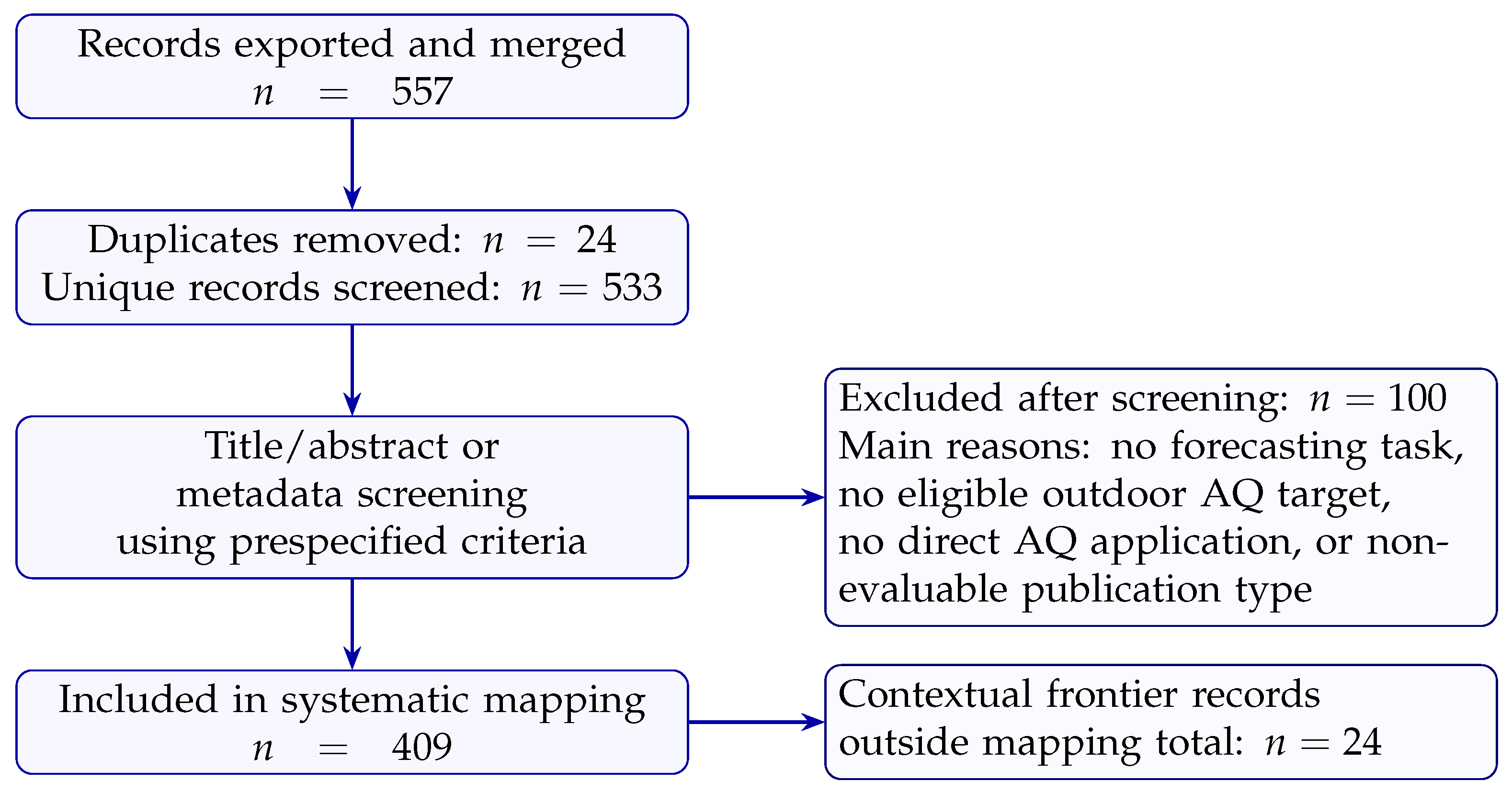
The merged database contained 557 records before deduplication. Twenty-four duplicate records were removed by DOI, arXiv identifier, or normalised title, leaving 533 unique records for screening. Applying Table 2, 409 records were retained in the forecasting map. A further 24 were kept outside the mapping total as contextual or frontier-method references because they informed atmospheric AI but did not establish a direct air-quality forecasting application. The remaining 100 were excluded, mainly because they lacked a forecasting/nowcasting task, an eligible outdoor air-quality target, a direct air-quality application, or an evaluable full publication. Figure 1 reports the selection process.

Figure 1. Screening flow for the systematic mapping review. Targeted full-text checks were used for ambiguity resolution and synthesis.

The included records were mapped along the dimensions defined by the research questions: target pollutant or air-quality indicator, model family, input-data source, temporal and spatial design, validation protocol, evaluation metric, interpretability, uncertainty treatment, and operational relevance. Because many bibliographic records did not include abstracts or full methodological descriptions, the resulting taxonomy should be interpreted as a conservative metadata-based classification. Full-text verification was used for representative studies discussed in detail and is recommended before using individual record-level classifications for secondary analyses.

The metadata map shows where the literature is concentrated, but it also shows what bibliographic records fail to reveal. General ML, recurrent DL, hybrid methods, and attention-based models are prominent, while explicit tags for rolling validation, forecast horizon, station geometry, uncertainty, and exceedance performance are uncommon. The latter absence is a reporting limitation, not evidence that these practices were never used. For this reason, the counts above support statements about topical prevalence only; the comparative conclusions in later sections come from targeted full-text reading and are signposted as such.

The map also suggests a shift from isolated time-series prediction towards multi-source and spatially coupled systems. Monitoring data are increasingly combined with meteorology, traffic or land-use proxies, satellite retrievals, and CTM output, while graph and attention mechanisms are used to represent relationships across locations. This shift strengthens the need to report issue-time availability and to distinguish interpolation within a known network from forecasting at unseen times, stations, or regions.

3. Data Constraints That Shape Model Choice

The data layer determines what can be forecast and what can be claimed. A lag-only single-station model mainly exploits persistence and seasonality. A network model can also use spatial transport signals, while a CTM-coupled system may draw on forecast meteorology, emissions, and chemical fields. These are different information regimes and should not be compared as though they were interchangeable.

Three constraints recur in the full-text synthesis. First, pollutant behaviour matters: PM_2.5 mixes primary emissions, secondary formation, humidity effects, and long-range transport; O₃ depends strongly on radiation, temperature, precursor chemistry, and NO titration; NO₂ can vary over street-scale distances; and PM₁₀ is sensitive to dust and resuspension. Second, monitoring geometry matters. Dense urban networks can support graph or convolutional models, whereas sparse or irregular networks favour hierarchical, state-space, transfer, or physically informed approaches that represent uncertainty explicitly. Third, predictor latency matters. Reanalysis fields, retrospectively corrected satellite products, centred filters, and future observations may improve retrospective fits but are not valid operational inputs unless an equivalent forecast product exists at issue time.

Preprocessing should therefore be treated as part of the forecasting model. Gap filling, scaling, decomposition, feature selection, and hyperparameter tuning must be fitted within each training fold. Performing these operations once on the complete series can leak future information even when the final train/test split is chronological. At minimum, studies should report the target and averaging period, horizon, monitoring geometry, input variables and latency, missing-data treatment, training window, validation split, and comparator set.

The metadata counts in Table 5 identify broad data-source themes but do not provide a complete census of predictor availability. The decision framework below therefore uses those counts as indicative support and relies on targeted full-text evidence for operational recommendations.

Table 5. Metadata-derived taxonomic distribution of the 409 included records. Categories are non-exclusive.

Dimension	Category	Count	% of 409
Model family	General ML/benchmark	207	50.6
	Recurrent DL	109	26.7
	Hybrid/decomposition	60	14.7
	Transformer/attention	51	12.5
	Tree ensemble/boosting	48	11.7
	CNN/ConvLSTM	43	10.5
	Regression/SVR/kernel	31	7.6
	Classic statistical methods	26	6.4
	Graph neural network	13	3.2
	Physics-informed/CTM-coupled	7	1.7
Target pollutant/indicator	Multiple/air pollutants	349	85.3
	AQI	123	30.1
	PM2.5	84	20.5
	PM10	31	7.6
	NO2/NOx	20	4.9
	O3/ozone	14	3.4
	CO	8	2.0
	SO2	7	1.7
	VOC	1	0.2
Data source	Traffic/land use/emissions	78	19.1
	Ground stations/sensors	75	18.3
	Meteorology	36	8.8
	Satellite/remote sensing	11	2.7
	CTM outputs	1	0.2
Temporal design	Hourly/sub-daily	11	2.7
	Long-term/monthly	8	2.0
	Daily/multi-day	4	1.0
Spatial setting	Urban/multi-station	87	21.3
	Regional/gridded	21	5.1
	Station-based	4	1.0
Validation protocol	Benchmark comparison	5	1.2
	Cross-validation	4	1.0
	Rolling/walk-forward	1	0.2

Note: Percentages use all 409 included records as the denominator. A study may appear in several rows, so percentages within a dimension need not sum to 100%. Low percentages for temporal, spatial, and validation descriptors indicate limited metadata reporting; they do not imply that the remaining studies lacked those characteristics.

4. Problem-Oriented Evidence Synthesis and Model-Selection Framework

The same algorithm can be appropriate in one setting and poorly justified in another. We therefore organise the synthesis by pollutant, monitoring geometry, predictor availability, and intended generalisation before discussing individual model families.

4.1. Pollutant-Specific Forecasting Challenges

PM_2.5, PM₁₀, O₃, NO₂, SO₂, CO, and AQI differ in source mixture, lifetime, spatial gradient, and regulatory use. Table 6 summarises the practical consequence: the relevant predictors and failure modes change with the target, and average RMSE can conceal the episodes that matter most.

Table 6. Pollutant-specific forecasting constraints and modelling implications derived from the targeted full-text synthesis.

Target	Dominant Forecasting Difficulty	Predictors That Become Important	Failure Mode That Average RMSE May Hide
PM2.5	Mixed primary/secondary origin, aerosol water, boundary-layer trapping, smoke, and long-range transport	Pollutant/species lags, PBL height, humidity, wind, precipitation, fire/dust indicators, and CTM fields	Underprediction of winter stagnation, smoke, dust, or holiday-emission peaks
PM10	Coarse-mode resuspension and dust superimposed on fine aerosol	Wind, precipitation, soil/dust proxies, traffic/activity, and dust or CTM forecasts	Missed dust intrusions or mechanically generated peaks
O3	Nonlinear photochemistry, NO titration, regional transport, and strong diurnal cycles	Radiation, temperature, NOx/VOC proxies, PBL and wind, upwind O3, and chemical-model output	Correct mean cycle but missed afternoon maxima or exceedance risk
NO2	Short lifetime, traffic gradients, and street-scale mixing	Traffic profiles, wind and stability, nearby-station topology, and co-pollutants	Spatial smoothing that removes roadside peaks
SO2	Directional point-source or shipping plumes and many low-concentration hours	Source-operation proxies, wind sector, plume-rise, and CTM information	Large plume errors diluted by quiet periods
CO	Strong traffic/heating cycles and regional background	Activity proxies, boundary-layer depth, wind, and co-pollutants	High correlation dominated by seasonality while short episodes are missed
AQI	Piecewise transformation controlled by the maximum pollutant sub-index	Forecasts for each constituent pollutant and local breakpoint definitions	Correct class for the wrong pollutant or discontinuous errors near thresholds

4.2. Decision Matrix: From Data Regime to Defensible Model

Table 7 gives a starting tier rather than a winner. The support column uses the non-exclusive family counts from the metadata map. It indicates how much literature is associated with the relevant family, not how many studies directly tested the exact recommendation. Where the mapping did not include a dedicated tag, we report that limitation instead of inferring a count.

Table 7. Decision matrix linking forecasting settings to model tiers, indicative mapped support, and minimum validation evidence.

Forecasting Setting	First Defensible Tier	Indicative Support in Map	Minimum Validation Evidence
One station; short or incomplete record	Persistence/seasonal naive, ARIMA/state-space, regularised regression, or tree boosting with a small issue-time feature set	Statistical $n=26$; regression/kernel $n=31$; trees $n=48$	Rolling origin after all preprocessing; persistence comparison; event-conditioned scores
Sparse network; heterogeneous missingness	Hierarchical/state-space model, local boosted trees, or transfer model with station descriptors; CTM/satellite covariates when operationally available	Statistical $n=26$; trees $n=48$; physics/CTM $n=7$	Temporal plus leave-site-out tests; results stratified by density and missingness
Dense multi-station network	Strong tabular/temporal baseline followed by GNN, ConvLSTM, or spatiotemporal attention	Recurrent $n=109$; CNN/ConvLSTM $n=43$; attention $n=51$; GNN $n=13$	Blocked temporal and leave-site/region-out tests; adjacency ablation; physical-unit errors
Regional grid with operational CTM	Calibrated CTM baseline followed by statistical or neural bias correction	Physics/CTM $n=7$; CNN/ConvLSTM $n=43$	Future-period or external-episode validation against CTM and persistence; bias and calibration
Rare exceedance warning	Quantile or probabilistic model, calibrated ensemble, or CTM-guided hybrid	No dedicated metadata code; targeted full-text evidence	POD, FAR, CSI, Brier/CRPS, and reliability in addition to MAE/RMSE; threshold fixed before testing
Transfer to a new city or region	Physics-guided predictors, hierarchical/domain-adaptation model, or pretrained model with local calibration	No dedicated transfer tag; spatial families provide indirect support	Leave-one-region-out or external-network test; recalibration separated from zero/few-shot transfer
Resource-constrained service	Parsimonious statistical/tree model or compact postprocessor	Statistical $n=26$; trees $n=48$	Accuracy–latency–memory comparison on deployment hardware

Complexity should be increased only when the additional data source or representation changes the information available to the model and improves the intended generalisation test. More parameters alone are not a sufficient reason to move beyond the first tier.

4.3. Sparse Monitoring as a Distinct Generalisation Problem

Sparse monitoring is not simply a smaller version of dense-network forecasting. Missingness is structured, station siting is selective, and a learned spatial graph may have too few informative neighbours. Hierarchical and state-space models can borrow strength while propagating uncertainty; tree ensembles remain useful when reliable meteorological, land-use, satellite, or CTM predictors are available; and transfer learning is credible only when source and target regions are separated in validation. A random record-wise split cannot establish robustness to an unseen station or region.

The practical rule is staged: establish persistence, seasonal, statistical, and tabular baselines; add deep or spatial structure only when the data geometry supports it; and retain the more complex model only if it improves the intended temporal, spatial, or external test. This prevents interpolation within a familiar network from being presented as evidence for deployment in a new one.

5. Evidence Base I: Statistical and Tabular Models

The metadata map contains 26 records tagged as classical statistical methods, 31 as regression/SVR/kernel methods, and 48 as tree ensembles. These overlapping counts do not rank performance, but they show that transparent and data-efficient approaches remain a substantial reference tier.

5.1. Transparent Temporal Baselines

Persistence, seasonal-naive forecasts, ARIMA/SARIMA, state-space models, and additive decompositions quantify how much skill follows from autocorrelation, trend, and recurring cycles alone [9,10,11]. Their main scientific value is diagnostic: a flexible model that does not beat a properly specified baseline under rolling validation has not demonstrated useful added value. State-space and Bayesian hierarchical formulations are especially attractive when observations are irregular or sparse because they separate process and measurement uncertainty. VAR/VARMA can incorporate several pollutants or meteorological series, but parameter growth is rapid and predictive lag relationships should not be read as chemical causality. GARCH-type extensions can represent clustered residual variance, although they cannot recover an emission or transport event absent from the inputs.

5.2. Tabular Machine Learning

Regularised regression, SVR, Random Forest, and gradient boosting are strong choices when the predictor set is mixed and the sample is too limited for a large neural model [12,13,14,15]. Tree ensembles are particularly effective with pollutant lags, calendar variables, meteorology, land use, and source proxies, while SVR can remain competitive in small to medium datasets. Their limitations are equally important: none provides a physical spatial representation by default, and all can exploit leaked preprocessing or unavailable predictors if the validation design is weak.

Stacking and weighted ensembles are common responses to site-to-site heterogeneity, but aggregation does not guarantee better extreme-event forecasts. Explainability tools such as SHAP can help identify influential predictors [16,17,18]; however, an explanation of a leaked or non-operational model remains non-operational. Spatiotemporal land-use regression and related hybrids can provide strong spatial estimates [19], yet interpolation skill within sampled locations should be kept distinct from future-time or unseen-site forecasting.

6. Evidence Base II: Temporal Deep Models

Recurrent deep learning is prominent in the metadata map ($n=109$), often as one component of a larger hybrid. LSTM and GRU models are well suited to long pollutant and meteorological sequences, while temporal convolutional networks offer a parallel, non-recurrent route to multi-scale lag structure [20,21,22]. Their advantage over tabular models is most plausible when the record is long, the input window contains informative dynamics, and the evaluation is chronological.

The full-text evidence does not support treating LSTM or GRU as automatic upgrades. Reported absolute errors are tied to pollutant range, station network, horizon, and split design [23,24]. Compact recurrent models can be effective for multi-horizon forecasts, but larger architectures are vulnerable to overfitting in short single-station records. They also cannot infer a sudden emission pulse or transport regime that is absent from the input sequence.

Regional extensions are more convincing when they add genuinely new information rather than capacity alone. For example, broadcasting or convolutional recurrent layers can combine station histories with WRF–CMAQ or gridded fields [25,26]. Such gains should be attributed jointly to the architecture, spatial support, and physical predictors, and should be tested at unseen times and locations.

7. Evidence Base III: Spatial, Attention, and Graph Models

Transformer/attention models ($n=51$) and GNNs ($n=13$) are smaller but rapidly growing categories. Attention can represent long temporal dependencies and interactions among variables; graph models encode stations or regions as nodes connected by distance, wind, learned adjacency, or physically motivated relations [27,28]. These capabilities are relevant when the task is genuinely multi-station or gridded.

The targeted synthesis nevertheless shows that architecture names alone are uninformative. Informer, Autoformer, FEDformer, TFT, PatchTST, and air-quality-specific attention variants differ in how they reduce sequence cost, represent periodicity, select variables, or generate multi-horizon outputs [29,30,31,32,33]. Their operational value depends on whether the same predictors are available in real time and whether gains survive comparison with strong recurrent and boosted-tree baselines. The HEART study is best read as targeted attention augmentation of an operational pipeline, not as evidence that attention is universally superior [34].

GNNs become scientifically persuasive when the graph reflects transport or chemistry and when validation leaves stations or regions out. GC-LSTM, adaptive graph models, and physics-guided graphs illustrate the range of available designs [28,35,36,37,38]. Randomly splitting records from the same stations mainly tests interpolation through familiar network structure; it does not show that the graph will transfer to a sparse or unseen network.

8. Evidence Base IV: Hybrid and Physically Coupled Models

Hybrid and decomposition methods are common in the map ($n=60$) because air-quality series contain linear persistence, nonlinear meteorology, seasonality, spatial transport, and episodic forcing. ARIMA–neural hybrids, wavelet/EMD/VMD pipelines, and stacked learners divide this structure among components [39,40,41]. Their main methodological risk is leakage: decomposition, feature selection, and optimisation must be repeated within each training fold rather than fitted once to the complete series.

CNN–LSTM, ConvLSTM, and ConvGRU systems are most defensible for spatial fields or station networks that can be embedded on a grid [24,42,43,44]. They add little if the spatial representation is artificial or if the test set shares the same stations and periods as the training data.

The strongest rationale for added complexity often comes from physical coupling. CTM-derived fields supply transport, meteorology, emissions, and chemistry that a concentration-only model cannot reconstruct. Deep data fusion and neural bias correction can then learn residual structure rather than the entire atmospheric system from scratch [26,45,46]. In the reported MCDL example, correction gains were especially visible during severe pollution, but the result remains tied to the CTM, assimilation design, region, and episode set. A calibrated CTM and a simple postprocessor should therefore remain explicit comparators.

9. Frontier Models: Evidence Maturity and Limits

Frontier methods are strategically important but less mature in the map: only seven records were tagged as physics-informed or CTM-coupled, while several foundation, diffusion, and benchmark studies were retained as contextual material. The key distinction is whether a method has been tested directly on pollutant forecasting, demonstrated only in a proof-of-concept setting, or inferred to be relevant from a neighbouring atmospheric task.

Physics-informed neural networks can incorporate transport or chemistry constraints and fuse sparse monitors with satellite and model fields [47]. Their promise is greatest where observations are sparse but governing structure is informative. Their validation must still test boundary conditions, source uncertainty, spatial transfer, and whether the imposed physics improves forecasts rather than only interpolation.

Probabilistic and Bayesian approaches address a more immediate operational gap. Quantile regression, Bayesian neural networks, Monte Carlo dropout, conformal prediction, and probabilistic ensembles can provide intervals or exceedance probabilities [48,49,50,51]. Calibration during rare events and distribution shift remains the central test; narrow intervals are not useful when their coverage collapses during high-pollution episodes.

Spatiotemporal embeddings and residual networks can improve regional estimation by representing location and calendar structure explicitly [52]. As with graph models, sample-based, spatial, and temporal cross-validation answer different questions and should not be merged into a single claim of generalisation.

Latent Diffusion, Foundation Models, and Evidence Classification

Tomasi et al. [53] used latent diffusion to downscale ERA5 meteorological fields over Italy. This result is relevant to dispersion modelling, but it is not direct evidence for reactive-pollutant downscaling. An air-quality application would need emissions and chemistry, non-negativity and mass-relevant constraints, and evaluation of extremes and spatial gradients against CTM and interpolation baselines.

The Aurora foundation model demonstrates that a shared Earth-system representation can be fine-tuned for several forecasting tasks, including air-quality prediction [54]. Broad pretraining may improve data efficiency, but it does not remove the need for pollutant-specific calibration, comparison with local operational systems, uncertainty verification, and evaluation in sparsely monitored regions. Model scale is therefore not evidence of transferability by itself.

Table 8 uses three explicit criteria. Applied evidence requires a direct pollutant or AQI forecasting task with held-out quantitative evaluation. Experimental evidence also concerns air quality, but remains a proof of concept, benchmark, preprint, or evaluation with limited operational or external validation. Prospective evidence comes from a neighbouring atmospheric or generic time-series task and has not yet demonstrated pollutant forecasting. These labels describe the maturity of the evidence cited here, not the intrinsic quality of the method.

Table 8. Evidence-maturity classification for advanced methods and the criteria used to assign each category.

Maturity	Classification Criterion	Examples	Interpretation in This Review
Applied	Direct pollutant/AQI forecast with held-out quantitative evaluation	CTM bias correction, multi-station GNN/ConvGRU, PINN data fusion, Aurora fine-tuning	Compare with physical and statistical baselines; inspect temporal/spatial holdout, extremes, and calibration
Experimental	Direct air-quality task, but proof-of-concept, benchmark/preprint, or limited external/operational testing	HEART attention augmentation, AirQualityBench, recent foundation or time-series benchmarks	Useful for hypothesis generation; publication status and evaluation scope must remain explicit
Prospective	No direct pollutant forecast; relevance inferred from an atmospheric or generic modelling task	Meteorological latent-diffusion downscaling and generic language/time-series models	Do not describe as demonstrated air-quality forecasting; state the missing chemistry, emissions, and validation tests

10. Cross-Cutting Themes

10.1. Spatiotemporal Modelling Strategies

The spatial dimension adds an additional layer of difficulty to air-quality forecasting. Treating each monitoring site in isolation ignores the fact that advection and diffusion couple distant locations, and that episodes often emerge from regional-scale patterns rather than purely local conditions. For this reason, many recent approaches move from post hoc spatial interpolation (e.g., kriging or inverse distance weighting applied to time-series forecasts) towards architectures that learn temporal and spatial structure jointly, such as ConvLSTM, STGCN, HEART, and latent diffusion models operating on gridded fields or station graphs [4,55].

10.2. Interpretability

As models become more complex, interpretability becomes a practical requirement rather than a luxury. Tree-based methods naturally expose variable importance, while SHAP values [56,57] provide a unified way to quantify the contribution of individual predictors across a wide class of models, highlighting, for example, which meteorological drivers are most associated with high PM episodes. Attention mechanisms in Transformer and graph-based networks, when carefully analysed, offer a complementary view by revealing which lags, stations, or regions attract the model’s focus during specific events.

10.3. Uncertainty Quantification

A point forecast saying “PM₁₀ will be 55 μg m⁻³ tomorrow” is less useful to an air-quality manager than one that expresses a 70% probability of exceeding the daily limit value. In operational frameworks, calibrated uncertainty is essential because it converts model output into actionable risk communication. Techniques such as Monte Carlo dropout, deep ensembles, and conformal prediction have therefore been adapted to air-quality forecasting to provide calibrated prediction intervals and exceedance probabilities, particularly for regulatory thresholds. Generative approaches, including diffusion models, further encourage an ensemble-based view in which multiple plausible trajectories are sampled, allowing users to reason about risk rather than only about point forecasts.

10.4. Multi-Task and Transfer Learning

Many air-quality applications share a common structure but differ in details such as pollutant mix, monitoring density, or emission regimes. Multi-task learning exploits these commonalities by predicting several pollutants or lead times simultaneously, which tends to improve generalisation through shared representations and cross-horizon regularisation. Transfer learning pushes this idea further by adapting models trained in data-rich regions to data-scarce settings, reducing cold-start problems for new networks or developing urban areas [4,58].

10.5. Benchmarking, Reproducibility, and Leakage Control

The systematic mapping makes clear that evaluation design is one of the least consistently reported aspects of the literature. Many metadata records identify a model family and target pollutant, but not the forecast horizon, temporal split, or predictor latency. This is not a minor reporting issue: random splits can overestimate performance when adjacent observations are strongly autocorrelated, and retrospective predictors can leak information that would not be available operationally. Future studies should therefore report the forecast issue time, lead time, training window, test window, hyperparameter-tuning strategy, and whether all predictors are available at issue time. Benchmark studies are especially useful when they enforce these constraints across model families [59,60].

10.6. Computational Efficiency

Operational services impose tight constraints on latency and computational cost, which often require dedicated workflow engines and virtual laboratories to orchestrate CTM runs, data assimilation, and postprocessing across heterogeneous HPC and cloud resources [61,62]. Efficient attention mechanisms, patch-based training strategies, and model–CTM hybrids that focus learning capacity on bias correction rather than full dynamics are promising ways to reconcile sophistication with the realities of production environments.

11. Evaluation Metrics as Decision Criteria

No single score captures operational forecast quality. MAE summarises typical absolute error, while RMSE places more weight on large misses. Bias reveals systematic over- or underprediction, and scale-free measures such as MASE can support comparisons across sites when the reference forecast is defined consistently [63,64]. Correlation or $R^2$ should not be reported alone because a model can reproduce variability while retaining substantial concentration bias.

When the objective is an alert, performance should also be conditioned on high concentrations or fixed thresholds. Probability of detection, false-alarm ratio, critical success index, and confusion matrices describe event discrimination. Probabilistic forecasts require calibration as well as sharpness, using Brier score, reliability diagrams, quantile loss, interval coverage, or CRPS [48,50,51]. The metric set should therefore follow the decision: average concentration forecasting, exceedance warning, spatial transfer, or uncertainty-aware planning.

12. Illustrative Case Study: Single-Station PM_2.5 Forecasting in Southern Italy

This experiment is a temporal stress test rather than part of the systematic map or a general benchmark. It asks three bounded questions under a common rolling protocol: whether complex learners improve on persistence and ARIMA for seven-day daily forecasts at one site; whether rankings change at high concentrations; and whether median aggregation improves average robustness without suppressing peaks. With one station, the experiment cannot test spatial transfer.

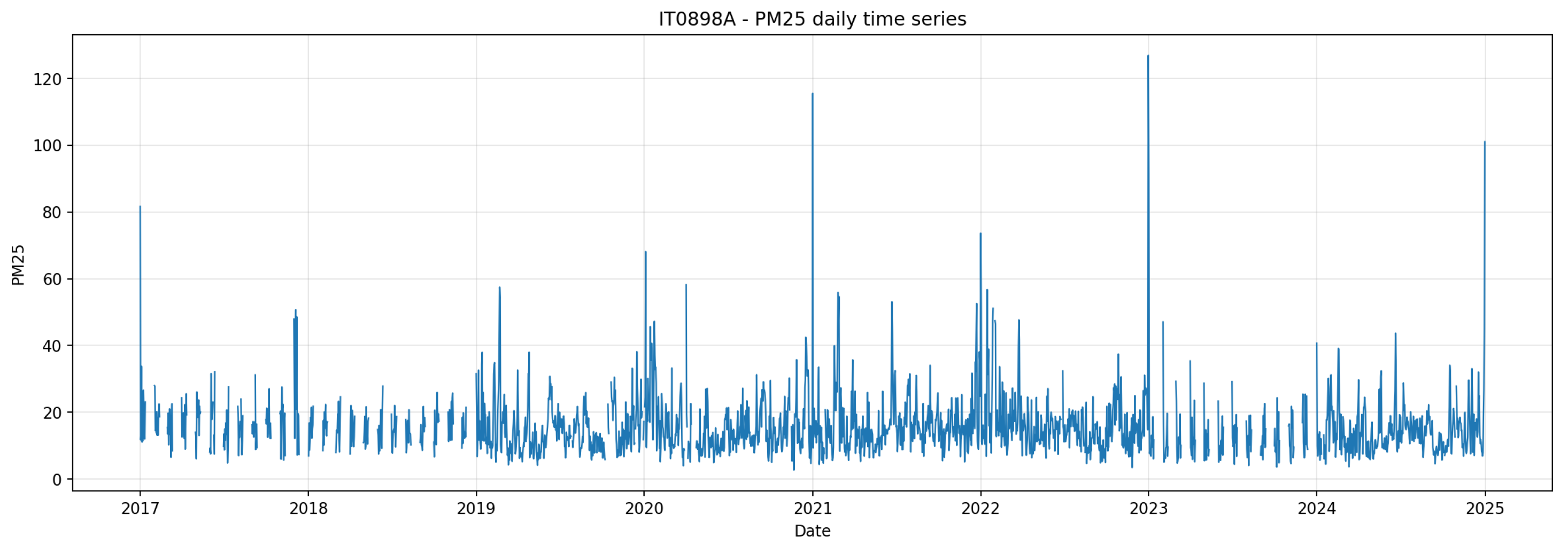
The target is the daily mean PM_2.5 concentration at EEA station IT0898, near the National Archaeological Museum in Naples (40.854167° N, 14.251111° E), over 2017–2025 (see Figure 2). The site is influenced by traffic, residential heating, regional transport, and intermittent Saharan dust [65,66]. It is a useful difficult case, but it is not statistically representative of Naples or of a monitoring network. Predictors were restricted to information available from the historical series and calendar at issue time; the comparison therefore tests lag-centred forecasting rather than a fully meteorological or CTM-informed system.

Figure 2. Daily PM_2.5 time series at station IT0898, showing seasonality, missing observations, and intermittent high-concentration episodes.

12.1. Experimental Design and Leakage-Safe Backtesting

Each fold used a contiguous historical training window and a seven-day future test window. The window then advanced, and all preprocessing, feature construction, fitting, and fallback rules were applied using training information only. This rolling-origin design produced 80 folds and 560 potential forecast cases before pairwise removal of missing observations. It is stricter than random splitting because it reproduces the information boundary faced by a forecaster.

All models were evaluated on the same folds using RMSE, MAE, bias, and MAPE. The same metrics were recomputed for observations above the station’s 50th, 75th, and 95th percentiles. Models that require explicit spatial topology or gridded physical fields—including GNNs, gridded ConvLSTM, PINNs, and CTM-coupled downscalers—were not fitted because the experiment contains only one concentration series.

12.2. Models and Implementation Scope

The main text retains only the comparison logic. Detailed model descriptions, feature construction, fitting sequence, and ensemble rule are provided in Supplementary Methods S1–S3. The tested set includes persistence and ARIMA baselines; Random Forest and histogram gradient boosting; radial-basis-function SVR; compact LSTM, GRU, and Transformer comparators; and a transparent median ensemble of successfully fitted classical and tabular members. Configurations were deliberately modest because the purpose was to compare model classes under one leakage-safe protocol, not to stage an unrestricted hyperparameter competition. The deposited code remains the definitive source for executable settings.

12.3. Results: Average Performance and Pollution Episodes

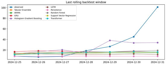
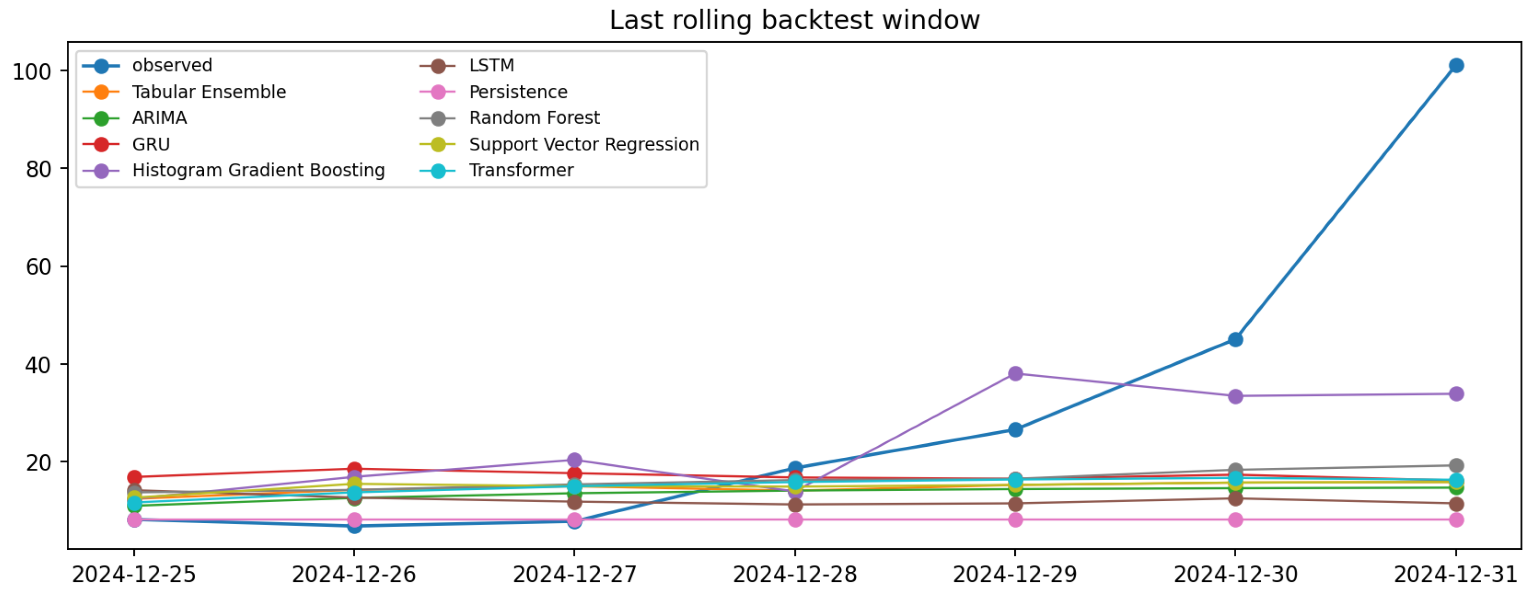
Figure 3 illustrates model behaviour during the last rolling backtest window, showing how the different algorithms track the evolution of a specific multi-day episode at the station. The final day in this window shows an abrupt concentration peak that coincides with New Year’s Eve and is plausibly influenced by firework emissions. Such emissions are episodic and are not encoded in the preceding daily concentration history, making the peak intrinsically difficult for purely autoregressive or lag-based forecasting models to reproduce. This example illustrates why average metrics can remain acceptable even when models underestimate rare extremes, and why episode-conditioned scores are essential for operational air-quality evaluation.

Figure 3. Comparison of observed daily PM_2.5 and selected forecasts during the final seven-day rolling window at station IT0898. The last-day peak coincides with New Year’s Eve and is plausibly influenced by a firework-related source that is absent from the lag-only feature set.

Table 9 summarises the performance of the completed model runs over all rolling backtest forecast cases, whereas Table 10 focuses only on high-concentration cases selected from the observed distribution. In Table 9, metrics are computed on $N=560$ pairs, i.e., 80 rolling folds × 7 forecast lead days. In Table 10, because the selection uses observed values above the threshold, the resulting counts are $N=257$ for P50, $N=131$ for P75, and $N=47$ for P95.

Table 9. Overall forecasting performance for daily PM_2.5 over the full rolling backtest. Metrics are computed on all valid observed–predicted pairs pooled across the 80 rolling folds and the seven forecast lead days. RMSE, MAE and Bias are all given in μg m⁻³.

Model	RMSE	MAE	Bias	MAPE (%)
Histogram Gradient Boosting	9.47	5.86	−0.03	41.04
Random Forest	9.90	5.76	−0.34	39.73
Tabular Ensemble	9.99	5.69	−0.63	38.50
GRU	10.10	5.78	−0.80	38.01
LSTM	10.11	5.74	−0.64	38.34
Support Vector Regression	10.15	5.64	−1.01	36.89
Persistence	10.78	6.42	−1.11	42.56
ARIMA	10.85	6.35	−0.42	43.59
Transformer	10.98	6.62	−0.45	43.81

Table 10. Percentile-conditioned rolling backtest performance for high-concentration daily PM_2.5 episodes. Thresholds are computed from the observed station series, and N denotes the number of rolling backtest forecast cases whose observed value exceeds the corresponding percentile threshold. Metrics are conditional on the selected subset and should be interpreted as episode-focused scores rather than averages over all 560 forecast cases. Threshold, RMSE, MAE and Bias are all given in μg m⁻³.

Model	Percentile	Threshold	N	RMSE	MAE	Bias	MAPE (%)
Histogram Gradient Boosting	P50	14.71	257	11.90	7.07	−5.21	25.07
Random Forest	P50	14.71	257	13.23	7.06	−6.01	22.94
Tabular Ensemble	P50	14.71	257	13.49	7.21	−6.19	23.51
LSTM	P50	14.71	257	13.61	7.54	−5.65	26.71
GRU	P50	14.71	257	13.68	7.80	−5.97	27.64
Support Vector Regression	P50	14.71	257	13.87	7.48	−6.30	25.17
Persistence	P50	14.71	257	14.13	8.26	−6.11	30.73
Transformer	P50	14.71	257	14.39	8.57	−6.04	29.95
ARIMA	P50	14.71	257	14.61	7.66	−7.01	23.44
Histogram Gradient Boosting	P75	19.22	131	16.18	11.10	−9.94	32.55
Random Forest	P75	19.22	131	18.29	11.69	−11.50	32.16
LSTM	P75	19.22	131	18.49	11.37	−10.57	32.01
GRU	P75	19.22	131	18.60	11.86	−11.20	33.61
Tabular Ensemble	P75	19.22	131	18.64	11.90	−11.80	32.73
Persistence	P75	19.22	131	18.90	11.73	−11.19	33.16
Support Vector Regression	P75	19.22	131	19.08	11.85	−11.67	32.59
Transformer	P75	19.22	131	19.55	13.28	−12.04	37.74
ARIMA	P75	19.22	131	20.35	13.44	−13.42	36.62
Histogram Gradient Boosting	P95	30.05	47	25.00	19.29	−19.22	40.91
LSTM	P95	30.05	47	29.28	20.74	−20.36	41.79
Random Forest	P95	30.05	47	29.29	22.53	−22.53	46.68
GRU	P95	30.05	47	29.31	21.71	−21.60	44.54
Persistence	P95	30.05	47	29.80	21.30	−21.30	42.62
Tabular Ensemble	P95	30.05	47	29.87	22.86	−22.86	47.24
Support Vector Regression	P95	30.05	47	30.54	23.00	−23.00	47.40
Transformer	P95	30.05	47	30.84	24.55	−24.55	51.49
ARIMA	P95	30.05	47	32.73	26.46	−26.46	55.81

When pooled across all seven lead days, histogram gradient boosting, Random Forest, SVR, and the median Tabular Ensemble improve on persistence and ARIMA in at least one principal error metric. Because Table 9 pools lead times, it does not by itself support a claim about how error changes with forecast horizon. The Tabular Ensemble remains close to the best overall MAE, but its advantage over the strongest individual members is small and does not extend to the P95 subset.

12.4. External Context and Limits of Generalisation

The Naples results estimate future-time performance for one instrument, local source mixture, and daily resolution. They do not estimate interpolation to an unmonitored site, robustness to a different station type, or transfer to another city. Multi-station studies address different questions and therefore provide context rather than a numerical validation of Table 9, Table 10 and Table 11.

Table 11. Comparison of the single-station experiment with representative multi-station or gridded benchmarks. Reported metrics are not pooled because the targets, horizons, and protocols differ.

Study Setting	Spatial/Forecast Design	What It Can Establish Beyond the Naples Experiment
Naples case study (this work)	One station; daily PM2.5; seven-day rolling windows	Temporal performance and high-percentile failure at this site; no spatial generalisation
Greater Bay Area [25]	Regional PM2.5/O3 forecasts using multiple stations and WRF–CMAQ information; 48 h	Benefit of spatial broadcasting and physical-model predictors within the evaluated regional network
Jing–Jin–Ji [28]	Station graph for PM2.5; forecasts to 72 h	Value of explicit inter-station dependence, subject to the reported spatial validation design
China MCDL [26]	Gridded CTM analysis and ConvGRU bias correction; three days	Performance of physically anchored spatiotemporal correction during a severe haze setting
AirQualityBench [59]	3720 stations, six pollutants, authentic missingness; global preprint benchmark	Robustness to fragmented monitoring coverage and the non-transferability of rankings from sanitised regional datasets

Generalisability would require a second experiment with several station types, leave-station-out testing, an external year or city, and predictors whose issue-time availability is identical across sites. The present case study is therefore retained because it demonstrates leakage-safe temporal evaluation and event underprediction, not because its numerical ranking can be exported to a network.

12.5. Discussion and Operational Insights

The contrast between the pooled scores in Table 9 and the percentile-conditioned scores in Table 10 is the main result of the case study. Histogram gradient boosting has the lowest overall RMSE (9.47 μg m⁻³), whereas SVR has the lowest overall MAE (5.64 μg m⁻³); the ranking therefore depends on the loss. More importantly, every model has a large negative bias in the P95 subset, from −19.22 to −26.46 μg m⁻³. Acceptable average error does not translate into reliable peak prediction.

The median ensemble remains close to the best average MAE but performs poorly at P95. In this experiment, aggregation dampens disagreement among members without repairing their shared underprediction of the upper tail. H1 is therefore supported for pooled average errors but not as a universal lead-specific statement; H2 is supported because rankings and biases change in the upper tail; and H3 is not supported for peak preservation.

These findings reinforce the decision framework. A strong boosted-tree or SVR baseline is difficult to beat on this short, lag-centred task, but none of the tested models contains enough information to anticipate an exogenous event such as a firework-related emission pulse. Better peak forecasts would require issue-time event indicators, meteorological or CTM predictors, an event-aware objective, or a calibrated probabilistic formulation. The case study diagnoses missing information; it does not establish a general hierarchy of algorithms.

13. Open Challenges and Future Directions

13.1. Long-Range and Extreme-Event Forecasting

Forecast skill tends to degrade quickly beyond 48–72 h, especially when the atmosphere transitions rapidly between regimes or when pollution episodes are triggered by sudden changes in emissions or long-range transport. Autoregressive decoding in deep sequence models accumulates small errors over time, and even physics-aware hybrids struggle to retain both sharpness and stability at longer lead times. Further progress will likely require architectures that embed more of the underlying transport and chemistry, for example by coupling deep networks more tightly with CTMs or by constraining latent dynamics through simplified physical models [55].

13.2. Domain Adaptation Across Urban Contexts

Most high-performing models are trained on dense networks in major cities or industrial regions, yet many policy-relevant questions arise in areas where observations are sparse or intermittent. Domain shifts in emission mixtures, meteorology, and land-use patterns make naive model transfer unreliable, often leading to biased or overconfident predictions. Spatiotemporal embedding strategies and PINN-based frameworks that assimilate satellite and reanalysis data offer promising tools for bridging this gap, but systematic methodologies for robust domain adaptation are still in their infancy.

13.3. High-Resolution Spatiotemporal Reconstruction

There is a growing demand for concentration fields at neighbourhood or street-canyon scale, driven by exposure assessment and urban planning. Traditional dynamical downscaling from CTMs at 3–15 km resolution to $\mathcal{O}\left(100\right)$ m grids is computationally demanding, which motivates the search for machine learning surrogates that can emulate small-scale variability. Latent diffusion models and U-Net-based fusion schemes that combine coarse CTM output with static and remote-sensing predictors are promising candidates, but their application to reactive air pollutants is only beginning to be explored [4].

13.4. Standardised Benchmarking

The literature on air-quality forecasting is rich in individual case studies but poor in shared benchmarks. Differences in datasets, evaluation windows, and metric choices make it difficult to assess whether a new model genuinely outperforms existing approaches or simply benefits from an easier testbed. Community efforts towards open, well-documented benchmark suites—analogous to the M-competitions in economic forecasting or to standard datasets in computer vision—would greatly clarify which advances are robust and which are context-dependent [64].

13.5. Integration with Numerical Weather Prediction

Finally, many of the most ambitious applications lie at the interface between machine learning and operational numerical weather prediction. Deep learning postprocessors can correct systematic biases and refine spatial detail in NWP and CTM outputs, while neural emulators offer the prospect of accelerating specific components such as radiation or chemistry. Realising this potential in an operational setting will require not only methodological innovation, but also careful attention to data assimilation, uncertainty propagation, and the constraints of real-time forecasting systems [55,67].

14. Conclusions

The metadata map and the targeted synthesis support different kinds of conclusions. From the metadata layer, the 409-record corpus is concentrated in general ML, recurrent DL, hybrid, attention, and tree-based studies, while explicit bibliographic reporting of rolling validation, station geometry, uncertainty, and event performance is sparse. These counts describe the literature’s emphasis; they do not establish which model family is most accurate.

From the targeted full-text synthesis, the defensible model depends on the pollutant, monitoring density, spatial support, forecast horizon, issue-time predictors, and intended generalisation claim. Statistical and tabular models remain the reference tier for short or sparse single-station records. Spatial deep models require informative network geometry and leave-site or leave-region-out evaluation. CTM-coupled correction is most compelling when forecast physical fields are available operationally. Probabilistic and event-conditioned evaluation is necessary when the decision concerns warnings rather than average reconstruction. Evidence for diffusion and foundation models is promising, but direct pollutant-specific and external validation remains uneven.

The revised decision matrix makes these recommendations more transparent by pairing each setting with indicative family counts from the map and with a minimum validation design. The counts are deliberately labelled non-exclusive and should be read as support for the breadth of an evidence family, not as votes for a recommendation. The Naples experiment provides a separate empirical illustration: there is no metric-independent winner, median ensembling does not preserve peaks, and every tested model underestimates the highest 5% of observations. In that setting, missing event and physical predictors matter more than additional architectural complexity.

The review is limited by its predominantly metadata-based map, targeted rather than uniform full-text appraisal, non-exclusive categories, and the absence of reason-specific exclusion counts in the original screening log. Cross-study metrics were therefore not pooled. The case study contains one urban station and cannot establish spatial transfer. Future work should combine open record-level screening data with issue-time-valid multi-station benchmarks, external-region tests, calibrated exceedance probabilities, and direct comparisons of physics-guided and pretrained models under sparse monitoring and distribution shift.

References

- World Health Organization. Ambient (Outdoor) Air Pollution. WHO Fact Sheet, 2024. Available online: https://www.who.int/news-room/fact-sheets/detail/ambient-(outdoor)-air-quality-and-health (accessed on 15 June 2026).
- Health Effects Institute; Institute for Health Metrics and Evaluation; UNICEF. State of Global Air Report 2024: A Special Report on Global Exposure to Air Pollution and its Health Impacts, with a Focus on Children’s Health; Technical Report; Health Effects Institute: Boston, MA, USA, 2024. [Google Scholar]
- World Health Organization. WHO Global Air Quality Guidelines: Particulate Matter (PM2.5 and PM10), Ozone, Nitrogen Dioxide, Sulfur Dioxide and Carbon Monoxide; Technical Report; World Health Organization: Bonn, Germany, 2021. [Google Scholar]
- Liao, Q.; Zhu, M.; Wu, L.; Pan, X.; Tang, X.; Wang, Z. Deep learning for air quality forecasts: A review. Curr. Pollut. Rep. 2020, 6, 399–409. [Google Scholar] [CrossRef] [Scilit]
- Kaur, M.; Singh, D.; Jabarulla, M.Y.; Kumar, V.; Kang, J.; Lee, H.N. Computational Deep Air Quality Prediction Techniques: A Systematic Review. Artif. Intell. Rev. 2023, 56, 2053–2098. [Google Scholar] [CrossRef] [Scilit]
- Agbehadji, I.E.; Obagbuwa, I.C. Systematic Review of Machine Learning and Deep Learning Techniques for Spatiotemporal Air Quality Prediction. Atmosphere 2024, 15, 1352. [Google Scholar] [CrossRef] [Scilit]
- Houdou, A.; El Badisy, I.; Khomsi, K.; Abdala, S.A.; Abdulla, F.; Najmi, H.; Obtel, M.; Belyamani, L.; Ibrahimi, A.; Khalis, M. Interpretable Machine Learning Approaches for Forecasting and Predicting Air Pollution: A Systematic Review. Aerosol Air Qual. Res. 2024, 24, 230151. [Google Scholar] [CrossRef] [Scilit] [PubMed]
- Yagnik, H.; Gupta, R.K.; Pandya, A. Deep Learning for Air Pollution Prediction: A Systematic Review of CNN, LSTM, GNN, and Transformer Architectures. Arch. Comput. Methods Eng. 2026. online first. [Google Scholar] [CrossRef] [Scilit]
- Box, G.E.; Jenkins, G.M.; Reinsel, G.C.; Ljung, G.M. Time Series Analysis: Forecasting and Control, 5th ed.; John Wiley & Sons: Hoboken, NJ, USA, 2015. [Google Scholar]
- Shumway, R.H.; Stoffer, D.S. Time Series Analysis and Its Applications: With R Examples, 4th ed.; Springer: Berlin/Heidelberg, Germany, 2017. [Google Scholar] [CrossRef] [Scilit]
- Taylor, S.J.; Letham, B. Forecasting at Scale. Am. Stat. 2018, 72, 37–45. [Google Scholar] [CrossRef] [Scilit]
- Vapnik, V.N. An Overview of Statistical Learning Theory. IEEE Trans. Neural Netw. 1999, 10, 988–999. [Google Scholar] [CrossRef] [Scilit] [PubMed]
- Breiman, L. Random Forests. Mach. Learn. 2001, 45, 5–32. [Google Scholar] [CrossRef] [Scilit]
- Chen, T.; Guestrin, C. XGBoost: A Scalable Tree Boosting System. In Proceedings of the 22nd ACM SIGKDD International Conference on Knowledge Discovery and Data Mining, San Francisco, CA, USA, 13–17 August 2016; pp. 785–794. [Google Scholar] [CrossRef] [Scilit]
- Ke, G.; Meng, Q.; Finley, T.; Wang, T.; Chen, W.; Ma, W.; Ye, Q.; Liu, T.Y. LightGBM: A Highly Efficient Gradient Boosting Decision Tree. In Proceedings of the Advances in Neural Information Processing Systems (NeurIPS), Long Beach, CA, USA, 4–9 December 2017; Volume 30, pp. 3146–3154. [Google Scholar]
- Gowri, L.; Sriya, N.S.; Sowmya, M.; Lakshmi, A.R.H.; Amirtharajan, R. Explainable AI for Urban Air Quality: SHAP Interpretation of Stacked Ensemble AQI Forecast. Theor. Appl. Climatol. 2025, 156, 533. [Google Scholar] [CrossRef] [Scilit]
- Ansari, A.; Quaff, A.R. Comparative Benchmarking of Eleven Machine Learning Regressors for Daily Air Quality Index (AQI) Forecasting: Sensitivity Analysis and SHapley Additive exPlanations (SHAP)-Based Interpretability Framework. Theor. Appl. Climatol. 2025, 156, 620. [Google Scholar] [CrossRef] [Scilit]
- Birinci, E.; Ekmekcioğlu, Ö.; Ozdemir, H.; Deniz, A. Interpretable Machine Learning Framework for Air Quality Prediction in Istanbul Using Shapley Additive Explanations (SHAP). Stoch. Environ. Res. Risk Assess. 2026, 40, 37. [Google Scholar] [CrossRef] [Scilit]
- Wang, J.; Xu, H. A novel hybrid spatiotemporal land use regression model system at the megacity scale. Atmos. Environ. 2021, 244, 117971. [Google Scholar] [CrossRef] [Scilit]
- Hochreiter, S.; Schmidhuber, J. Long Short-Term Memory. Neural Comput. 1997, 9, 1735–1780. [Google Scholar] [CrossRef] [Scilit] [PubMed]
- Cho, K.; van Merriënboer, B.; Gulcehre, C.; Bahdanau, D.; Bougares, F.; Schwenk, H.; Bengio, Y. Learning phrase representations using RNN encoder–decoder for statistical machine translation. arXiv 2014, arXiv:1406.1078. [Google Scholar]
- Bai, S.; Kolter, J.Z.; Koltun, V. An Empirical Evaluation of Generic Convolutional and Recurrent Networks for Sequence Modeling. arXiv 2018, arXiv:1803.01271. [Google Scholar]
- Zhao, J.; Deng, F.; Cai, Y.; Chen, J. Long short-term memory—Fully Connected (LSTM-FC) neural network for PM2.5 concentration prediction. Chemosphere 2019, 220, 486–492. [Google Scholar] [CrossRef] [Scilit] [PubMed]
- Huang, C.J.; Kuo, P.H. A deep CNN-LSTM model for particulate matter (PM2.5) forecasting in smart cities. Sensors 2018, 18, 2220. [Google Scholar] [CrossRef] [Scilit] [PubMed]
- Sun, H.; Fung, J.C.H.; Chen, Y.; Li, Z.; Yuan, D.; Chen, W.; Lu, X. Development of an LSTM broadcasting deep-learning framework for regional air pollution forecast improvement. Geosci. Model Dev. 2022, 15, 8439–8452. [Google Scholar] [CrossRef] [Scilit]
- Zhao, Z.; Wu, H.; Chen, K.; Kong, L.; Tang, X. Improving the Spatiotemporal Forecasting of PM2.5 by Coupling a Deep Learning Method with a Chemical Transport Model: A Severe Haze Case in China. Aerosol Sci. Eng. 2026, 10, 354–369. [Google Scholar] [CrossRef] [Scilit]
- Vaswani, A.; Shazeer, N.; Parmar, N.; Uszkoreit, J.; Jones, L.; Gomez, A.N.; Kaiser, L.; Polosukhin, I. Attention is All You Need. In Proceedings of the Advances in Neural Information Processing Systems (NeurIPS), Long Beach, CA, USA, 4–9 December 2017; Volume 30. [Google Scholar]
- Qi, Y.; Li, Q.; Karimian, H.; Liu, D. A hybrid model for spatiotemporal forecasting of PM2.5 based on graph convolutional neural network and long short-term memory. Sci. Total Environ. 2019, 664, 1–10. [Google Scholar] [CrossRef] [Scilit] [PubMed]
- Zhou, H.; Zhang, S.; Peng, J.; Zhang, S.; Li, J.; Xiong, H.; Zhang, W. Informer: Beyond Efficient Transformer for Long Sequence Time-Series Forecasting. In Proceedings of the AAAI Conference on Artificial Intelligence, Virtual Event, 2–9 February 2021; Volume 35, pp. 11106–11115. [Google Scholar] [CrossRef] [Scilit]
- Wu, H.; Xu, J.; Wang, J.; Long, M. Autoformer: Decomposition Transformers with Auto-Correlation for Long-Term Series Forecasting. In Proceedings of the Advances in Neural Information Processing Systems (NeurIPS), Virtual Event, 6–14 December 2021; Volume 34. [Google Scholar]
- Zhou, T.; Ma, Z.; Wen, Q.; Wang, X.; Sun, L.; Jin, R. FEDformer: Frequency Enhanced Decomposed Transformer for Long-term Series Forecasting. In Proceedings of the 39th International Conference on Machine Learning (ICML), Baltimore, MD, USA, 17–23 July 2022. [Google Scholar]
- Lim, B.; Arık, S.Ö.; Loeff, N.; Pfister, T. Temporal fusion transformers for interpretable multi-horizon time series forecasting. Int. J. Forecast. 2021, 37, 1748–1764. [Google Scholar] [CrossRef] [Scilit]
- Nie, Y.; Nguyen, N.H.; Sinthong, P.; Kalagnanam, J. A time series is worth 64 words: Long-term forecasting with transformers. arXiv 2022, arXiv:2211.14730. [Google Scholar]
- Bodendorfer, N. A HEART for the environment: Transformer-Based Spatiotemporal Modeling for Air Quality Prediction. arXiv 2025, arXiv:2502.19042. [Google Scholar]
- Wu, Z.; Pan, S.; Long, G.; Jiang, J.; Zhang, C. Graph WaveNet for Deep Spatial-Temporal Graph Modeling. In Proceedings of the 28th International Joint Conference on Artificial Intelligence (IJCAI), Macao, China, 10–16 August 2019; pp. 1907–1913. [Google Scholar] [CrossRef] [Scilit] [PubMed]
- Hettige, K.H.; Ji, J.; Xiang, S.; Long, C.; Cong, G.; Wang, J. AirPhyNet: Harnessing Physics-Guided Neural Networks for Air Quality Prediction. arXiv 2024, arXiv:2402.03784. [Google Scholar]
- Chen, L.; Xu, J.; Wu, B.; Lv, M.; Zhan, C.; Chen, S.; Chang, J. HighAir: A Hierarchical Graph Neural Network-Based Air Quality Forecasting Method. arXiv 2021, arXiv:2101.04264. [Google Scholar]
- Chen, L.; Xu, J.; Wu, B.; Qian, Y.; Du, Z.; Li, Y.; Zhang, Y. Group-Aware Graph Neural Network for Nationwide City Air Quality Forecasting. arXiv 2021, arXiv:2108.12238. [Google Scholar]
- Zhang, G.P. Time series forecasting using a hybrid ARIMA and neural network model. Neurocomputing 2003, 50, 159–175. [Google Scholar] [CrossRef] [Scilit]
- Torres, M.E.; Colominas, M.A.; Schlotthauer, G.; Flandrin, P. A complete ensemble empirical mode decomposition with adaptive noise. In Proceedings of the 2011 IEEE International Conference on Acoustics, Speech and Signal Processing (ICASSP), Prague, Czech Republic, 22–27 May 2011; pp. 4144–4147. [Google Scholar] [CrossRef] [Scilit]
- Dragomiretskiy, K.; Zosso, D. Variational Mode Decomposition. IEEE Trans. Signal Process. 2014, 62, 531–544. [Google Scholar] [CrossRef] [Scilit]
- Shi, X.; Chen, Z.; Wang, H.; Yeung, D.Y.; Wong, W.K.; Woo, W.C. Convolutional LSTM Network: A Machine Learning Approach for Precipitation Nowcasting. In Proceedings of the Advances in Neural Information Processing Systems (NeurIPS), Montréal, QC, Canada, 7–12 December 2015; Volume 28. [Google Scholar]
- Alléon, A.; Jauvion, G.; Quennehen, B.; Lissmyr, D. PlumeNet: Large-Scale Air Quality Forecasting Using a Convolutional LSTM Network. arXiv 2020, arXiv:2006.09204. [Google Scholar]
- Han, Y.; Zhang, Q.; Li, V.O.K.; Lam, J.C.K. Deep-AIR: A Hybrid CNN-LSTM Framework for Air Quality Modeling in Metropolitan Cities. arXiv 2021, arXiv:2103.14587. [Google Scholar]
- Lyu, B.; Huang, R.; Wang, X.; Wang, W.; Hu, Y. Deep-learning spatial principles from deterministic chemical transport models for chemical reanalysis: An application in China for PM2.5. Geosci. Model Dev. 2022, 15, 1583–1594. [Google Scholar] [CrossRef] [Scilit]
- Cai, S.; Fang, F.; Peuch, V.H.; Alexe, M.; Navon, I.M.; Wang, Y. Advancing Operational PM2.5 Forecasting with Dual Deep Neural Networks (D-DNet). arXiv 2024, arXiv:2406.19154. [Google Scholar]
- Li, B.; Hu, Q.; Gao, M.; Liu, T.; Zhang, C.; Liu, C. Physical informed neural network improving the WRF-CHEM results of air pollution using satellite-based remote sensing data. Atmos. Environ. 2023, 308, 120031. [Google Scholar] [CrossRef] [Scilit]
- Murad, A.; Kraemer, F.A.; Bach, K.; Taylor, G. Probabilistic deep learning to quantify uncertainty in air quality forecasting. Sensors 2021, 21, 8009. [Google Scholar] [CrossRef] [Scilit] [PubMed]
- Pian, Y.; Wang, T.; Zhang, S.; Xu, R.; Liu, Y. Tackling Incomplete Data in Air Quality Prediction: A Bayesian Deep Learning Framework for Uncertainty Quantification. arXiv 2025, arXiv:2511.02175. [Google Scholar]
- Borah, J.; Chakraborty, T.; Nadzir, M.S.M.; Cayetano, M.G.; Majumdar, S. WaveCatBoost for Probabilistic Forecasting of Regional Air Quality Data. arXiv 2024, arXiv:2404.05482. [Google Scholar]
- Zhang, B.; Hao, B.; Bai, W. Comparative Evaluation of LSTM, TCN, and Quantile Regression with Conformal Prediction for Time Series Forecasting under Uncertainty. In Proceedings of the CCAI, Haikou, China, 23–25 May 2025. [Google Scholar] [CrossRef] [Scilit]
- Li, T.; Cheng, X. Estimating daily full-coverage surface ozone concentration using satellite observations and a spatiotemporally embedded deep learning approach. Int. J. Appl. Earth Obs. Geoinf. 2021, 101, 102356. [Google Scholar] [CrossRef] [Scilit]
- Tomasi, E.; Franch, G.; Cristoforetti, M. Can AI be enabled to perform dynamical downscaling? A latent diffusion model to mimic kilometre-scale COSMO-5.0-CLM9 simulations. Geosci. Model Dev. 2025, 18, 2051–2078. [Google Scholar] [CrossRef] [Scilit]
- Bodnar, C.; Bruinsma, W.P.; Lucic, A.; Stanley, M.; Allen, A.; Brandstetter, J.; Garvan, P.; Riechert, M.; Weyn, J.A.; Dong, H.; et al. A foundation model for the Earth system. Nature 2025, 641, 1180–1187. [Google Scholar] [CrossRef] [Scilit] [PubMed]
- Reichstein, M.; Camps-Valls, G.; Stevens, B.; Jung, M.; Denzler, J.; Carvalhais, N.; Prabhat. Deep learning and process understanding for data-driven Earth system science. Nature 2019, 566, 195–204. [Google Scholar] [CrossRef] [Scilit] [PubMed]
- Lundberg, S.M.; Lee, S.I. A Unified Approach to Interpreting Model Predictions. In Proceedings of the Advances in Neural Information Processing Systems, Long Beach, CA, USA, 4–9 December 2017; Volume 30. [Google Scholar]
- Lundberg, S.M.; Erion, G.; Chen, H.; DeGrave, A.; Prutkin, J.M.; Nair, B.; Katz, R.; Himmelfarb, J.; Bansal, N.; Lee, S.I. From local explanations to global understanding with explainable AI for trees. Nat. Mach. Intell. 2020, 2, 56–67. [Google Scholar] [CrossRef] [Scilit] [PubMed]
- Ma, J.; Cheng, J.C.; Lin, C.; Tan, Y.; Zhang, J. Improving air quality prediction accuracy at larger temporal resolutions using deep learning and transfer learning techniques. Atmos. Environ. 2019, 214, 116885. [Google Scholar] [CrossRef] [Scilit]
- Xu, X.; Wang, X.; Zhang, Y.; Zhao, H.; Zhou, Z.; Wang, Y. AirQualityBench: A Realistic Evaluation Benchmark for Global Air Quality Forecasting. arXiv 2026, arXiv:2605.05854. [Google Scholar]
- Gondal, M.U.; Qudous, H.u.; Farhan, A.A.; Alamri, S. Interpretable PM2.5 Forecasting for Urban Air Quality: A Comparative Study of Operational Time-Series Models. arXiv 2026, arXiv:2603.25495. [Google Scholar]
- Ascione, I.; Giunta, G.; Mariani, P.; Montella, R.; Riccio, A. A grid computing based virtual laboratory for environmental simulations. In Proceedings of the European Conference on Parallel Processing; Springer: Berlin/Heidelberg, Germany, 2006; pp. 1085–1094. [Google Scholar]
- Giunta, G.; Mariani, P.; Montella, R.; Riccio, A. pPOM: A nested, scalable, parallel and Fortran 90 implementation of the Princeton Ocean Model. Environ. Model. Softw. 2007, 22, 117–122. [Google Scholar] [CrossRef] [Scilit]
- Hyndman, R.J.; Koehler, A.B. Another look at measures of forecast accuracy. Int. J. Forecast. 2006, 22, 679–688. [Google Scholar] [CrossRef] [Scilit]
- Masud, K.I.; Unnam, V.S.R.; Ali, S. Benchmarking Scientific Machine Learning Models for Air Quality Data. arXiv 2026, arXiv:2603.21039. [Google Scholar]
- Riccio, A.; Barone, G.; Chianese, E.; Giunta, G. A hierarchical Bayesian approach to the spatio-temporal modeling of air quality data. Atmos. Environ. 2006, 40, 554–566. [Google Scholar] [CrossRef] [Scilit]
- Giarra, A.; Riccio, A.; Chianese, E.; Annetta, M.; Toscanesi, M.; Trifuoggi, M. Transport Mechanisms and Pollutant Dynamics Influencing PM10 Levels in a Densely Urbanized and Industrialized Region near Naples, South Italy: A Residence Time Analysis. Atmosphere 2025, 16, 393. [Google Scholar] [CrossRef] [Scilit]
- Bauer, P.; Thorpe, A.; Brunet, G. The quiet revolution of numerical weather prediction. Nature 2015, 525, 47–55. [Google Scholar] [CrossRef] [Scilit] [PubMed]
- Camastra, F.; Capone, V.; Ciaramella, A.; Riccio, A.; Staiano, A. Prediction of environmental missing data time series by Support Vector Machine Regression and Correlation Dimension estimation. Environ. Model. Softw. 2022, 150, 105343. [Google Scholar] [CrossRef] [Scilit]
Disclaimer/Publisher’s Note: The statements, opinions and data contained in all publications are solely those of the individual author(s) and contributor(s) and not of MDPI and/or the editor(s). MDPI and/or the editor(s) disclaim responsibility for any injury to people or property resulting from any ideas, methods, instructions or products referred to in the content. |
© 2026 by the authors. Licensee MDPI, Basel, Switzerland. This article is an open access article distributed under the terms and conditions of the Creative Commons Attribution (CC BY) license.