


Highlights
What are the main findings?
- The proposed panel-based framework evaluates HEI financial risk as a multi-class temporally validated early-warning task, integrating revenue-structure, expenditure-pressure, financial-health, and institutional/contextual indicators.
- Financial-health indicators provide the strongest direct classification signal, whereas broader multidimensional indicators mainly improve contextual interpretation and governance relevance rather than substantially increasing point-classification performance.
What are the implication of the main finding?
- HEI financial risk early warning should move beyond static ratio-based assessment by combining panel-data modeling, temporal and institutional validation, leakage-aware evaluation, class-balanced performance metrics, and interpretable risk evidence.
- RPA can serve as a traceable execution layer rather than a forecasting model, supporting the conversion of risk classifications into standardized alerts, review procedures, responsibility assignment, audit trails, and feedback-based governance updates.
Abstract
High classification performance in financial-risk early-warning research may reflect recovery of a constructed contemporaneous rating rule rather than prediction of an independent future outcome. This study distinguishes these two forms of evidence through a controlled synthetic-panel experiment situated in the context of higher education institutions (HEIs). Task 1 is a contemporaneous positive-control audit in which the four components defining a deterministic three-class rating are supplied to the classifiers. Task 2 uses predictors measured at year to classify the rating at year t through strict rolling-origin evaluation under prespecified Weak, Moderate, and Strong temporal-persistence conditions. In Task 1, the four fitted classifiers achieved held-out Macro-F1 values of 0.9968–1.0000, demonstrating near-complete recovery of the disclosed rating rule but providing no prospective forecasting evidence. In Task 2, the best mean annual Macro-F1/Macro-AUC increased from 0.480/0.696 under Weak persistence to 0.549/0.747 under Moderate persistence and 0.633/0.824 under Strong persistence. The Weak–Moderate–Strong ordering was observed for both primary metrics across all four fitted classifiers, while higher model complexity provided no consistent advantage within the disclosed synthetic mechanism. These findings confirm contemporaneous rule recoverability and sensitivity to deliberately embedded temporal persistence only within the controlled experiment. They do not establish predictive validity, transportability, or decision benefit in real HEIs. The study contributes a reproducible task-to-claim approach that aligns target construction, predictor–target overlap, information timing, rolling-origin evaluation, probability quality, and model performance with the inferences that the resulting evidence can legitimately support. Real-world validation would require source-indexed longitudinal HEI data, independently adjudicated post-origin outcomes, verified information-availability dates, external testing, and prospective decision evaluation.
1. Introduction
Higher education institutions (HEIs) operate under changing conditions of enrollment, funding, expenditure, and accountability. Their financial sustainability is therefore shaped by both internal resource structures and external institutional pressures [1,2,3]. Financial monitoring can support the timely identification of vulnerability and the prioritization of professional review [4,5]. However, the evidential meaning of such monitoring depends on the relationship among outcome definition, predictor timing, validation design, and intended use.
The distinction between current-state classification and early warning is especially important. Early warning requires predictors available before a defined forecast origin and an outcome observed after that origin [6,7,8]. A contemporaneous rating may summarize current financial conditions [9], but it does not by itself demonstrate advance prediction. If variables used to construct a rating are also supplied to a classifier, a high performance may reflect the recovery of the rating rule rather than prediction of an independent later outcome [10,11,12]. A random held-out split cannot resolve this information-timing problem when target construction overlaps with the predictors. Prospective claims therefore require explicit temporal alignment and evaluation on later untouched periods [13,14].
This distinction is also consequential for machine-learning comparisons. Flexible models can approximate nonlinear thresholds and interactions more closely than restrictive parametric specifications [15], but algorithmic complexity cannot create temporal validity or outcome independence. The apparent performance may also depend on the persistence of the underlying process: a lagged predictor should be more informative when the preceding state is more strongly carried into the next period. Without a controlled mechanism, however, the effects of target overlap, temporal persistence, data quality, and model flexibility are difficult to distinguish.
To isolate these validity problems, the present study uses a fully disclosed synthetic-panel experiment as a methodological test bed. Simulation studies are appropriate when a known data-generating mechanism is required to isolate method behavior under controlled conditions [16,17]. The purpose of the experiment is not to estimate the prevalence of financial risk among HEIs but to vary a known temporal mechanism while retaining complete control over target construction and information timing. Three balanced panels represent Weak, Moderate, and Strong temporal-persistence conditions, with the persistence coefficient fixed at , , and , respectively. Each panel contains 3000 neutral synthetic units observed annually from 2015 to 2025. The three scenarios reuse the same units and random-number stream, with only varying across scenarios. This common-random-number strategy supports a more controlled comparison of the three prespecified conditions [18]. The experiment neither reproduces nor samples the financial conditions of identifiable HEIs. Public higher-education and financial materials inform only the broad interpretation of the synthetic variables.
The study objective is to determine how predictor–target overlap and prespecified temporal persistence affect the performance and interpretation of multiclass financial-risk classification within a reproducible controlled design. Two analytical tasks establish distinct evidence boundaries. Task 1 supplies the four same-year components used to construct a deterministic three-class rating and tests whether fitted classifiers recover that rule on held-out synthetic units. It is a positive-control audit rather than a forecasting test. Task 2 uses 12 predictors measured at year to classify the rating at year t through expanding-window rolling-origin evaluation across eight test years from 2018 to 2025. Task 2 therefore evaluates one-year-ahead predictability within the disclosed synthetic mechanism, but it does not establish real-world HEI early-warning performance.
Against this background, the study addresses two research questions:
- RQ1.
- To what extent can the deterministic three-class rating be recovered when its four target-defining components are supplied contemporaneously to the classifiers, and what does this reveal about the interpretation of target-inclusive performance?
- RQ2.
- How do one-year-ahead classification performance, discrimination, probability quality, and annual stability vary across prespecified Weak, Moderate, and Strong temporal-persistence conditions under rolling-origin evaluation, and do the four fitted classifiers exhibit the same scenario ordering on the two primary metrics?
Table 1 connects the research questions with their corresponding analytical tasks, evidence, and claim boundaries.
Table 1.
Alignment of research questions, analytical tasks, and evidential boundaries.
The study makes three bounded contributions. First, it provides a controlled demonstration of why target-inclusive same-year classification must be distinguished from fixed-horizon prediction. Second, it shows how a common-random-number design can isolate the effect of prespecified temporal persistence while holding synthetic units and innovation streams constant. Third, it links task definition to prespecified primary and complementary metrics, annual evaluation, archived probability outputs, and explicit claim boundaries within a reproducible reporting design. These contributions are methodological: the study provides neither a sectoral estimate of HEI financial risk nor validation of an operational early-warning system.
Any future use of automated workflows for data checks, version control, case routing, or audit recording would require separate prospective operational and decision-focused validation under accountable human oversight [19,20,21,22,23]. Automation cannot validate a constructed outcome, convert synthetic evidence into empirical validity, or replace professional judgement.
The remainder of the paper is organized as follows. Section 2 reviews early-warning validity, predictor–target overlap, temporal evaluation, and comparative model assessment and then develops the conceptual framework and prespecified checks. Section 3 specifies the synthetic data-generating process, the deterministic rating, analytical variables, integrity audits, Task 1 and Task 2 designs, model configurations, evaluation measures, and reproducibility controls. Section 4 reports the integrity checks, scenario diagnostics, task-specific performance, annual Task 2 results, and the contrast between Tasks 1 and 2. Section 5 interprets the findings and defines a staged path from synthetic experimentation to empirical and operational validation. Section 6 summarizes the principal findings, methodological contributions, and evidential boundaries.
2. Literature Review and Conceptual Framework
This section develops the conceptual basis for the controlled experiment. It first distinguishes financial monitoring from prospective early warning. It then examines constructed outcomes and predictor–target overlap, temporal persistence and rolling-origin validation, and the relationship among model flexibility, discrimination, and probability quality. The section concludes by synthesizing these issues into a conceptual framework and two prespecified checks that guide the subsequent methods and interpretation.
2.1. HEI Financial Monitoring and Prospective Early Warning
HEI financial monitoring commonly considers liquidity, solvency, budgetary control, revenue structure, and broader financial sustainability [24,25]. These dimensions are institutionally consequential, because resource and revenue structures are associated with credit assessment and academic output [26], as well as research capacity and institutional competitiveness [27,28]. Institutional and contextual information may also assist in interpretation, because HEIs differ in scale, mission, funding exposure, and operating environments [29].
HEI studies commonly analyze annual financial and institutional records [25,30]. In such applications, however, the year attached to a record is not necessarily the date on which that information became available for prediction. Failure to distinguish the observation period, release date, forecast origin, and outcome period can introduce look-ahead bias or target leakage. Researchers may also use expert- or threshold-based ratings as tractable outcomes. Such ratings can support current-state monitoring, but their construction must be disclosed, and their defining inputs must not be mistaken for independent predictors [31].
Substantive relevance does not determine predictive status. A measure observed in the same period as a rating can describe the current conditions, support rule-consistency monitoring, or inform professional review. Early-warning evidence is narrower: predictors must be available before a defined forecast origin, and the outcome must be observed after that origin. A multi-year panel can support temporal analysis, but longitudinal structure alone does not guarantee prospective validity [32]. The observation time, reporting time, and model-availability time of each field must therefore be distinguished.
This study consequently treats “early warning” as an evidential claim rather than a label that can be attached to any financial classifier. Task 1 is a contemporaneous rule-recovery audit. Task 2 imposes a one-year information boundary, but its outcome remains synthetic and rule-derived. Task 2 is therefore methodologically closer to forecasting, while remaining insufficient to support claims about actual institutional distress or real-world HEI early-warning performance.
2.2. Constructed Outcomes, Target Overlap, and Positive-Control Audits
Outcome construction is a measurement decision. A researcher-defined rating is reproducible only when its components, thresholds, class order, overrides, and boundary conditions are disclosed. If those components are subsequently reused as model inputs, predictor–target overlap is created. Flexible classifiers may then achieve very high held-out performance, because the construction rule remains stable across the split and not because the inputs independently anticipate a later event. This form of label leakage can produce overly optimistic interpretations [33].
Holding out units does not remove this circularity. Although the records in the test subset are unseen during model fitting, the same deterministic relationship connects the predictors to the labels in both the fitting and test subsets. Target-inclusive classification can nevertheless serve as a positive-control audit. Successful recovery verifies that the analytical pipeline can learn the embedded rule and reveals the performance ceiling created by direct predictor–target overlap. Its value depends on naming the task correctly and preventing the resulting performance from being presented as evidence of advance warning.
This distinction also clarifies the role of multidimensional indicators. Revenue, expenditure, financial ratios, institutional descriptors, and contextual variables may all be relevant to financial monitoring [34,35], but indicator breadth alone does not establish predictive value. Prospective evidence depends on target independence, predictor availability before the forecast origin, and performance in later untouched periods.
2.3. Temporal Persistence and Rolling-Origin Evaluation
One-year-ahead classification depends partly on temporal persistence. When a latent financial state is weakly persistent, measurements from year may contain limited information about a rating in year t. Stronger persistence should increase that information when other elements are held constant. In real data, however, temporal persistence is entangled with measurement error, institutional heterogeneity, policy change, and unobserved shocks. A controlled synthetic experiment can vary the persistence directly, but the resulting scenario ordering constitutes a mechanism check rather than an estimate of real HEI behavior [36].
Validation must respect the same temporal logic. Random splitting may mix earlier and later observations and does not emulate prospective use. Rolling-origin evaluation instead fits models using the historical information available at a given forecast origin, uses a later validation period for configuration selection, and evaluates the selected configuration on the next untouched period [37]. Repeating this process across successive forecast origins can reveal annual instability that a single pooled score may conceal.
Repeated longitudinal predictions also require an appropriate unit of inference. Predictions for the same synthetic units, test years, and common-random-number scenarios are dependent. Record-level tests that treat all saved predictions or probabilities as independent observations can create pseudoreplication. Annual test periods, effect magnitudes, and scenario-consistent patterns therefore provide the defensible basis for inference in the present design [38].
2.4. Model Flexibility, Discrimination, and Probability Quality
Financial-risk research increasingly compares statistical and machine-learning classifiers, because nonlinear learners can represent thresholds and interactions in structured data [39]. Multinomial logistic regression provides an interpretable linear benchmark, a decision tree represents recursive thresholding, and bagging and adaptive boosting provide two established ensemble strategies [40,41]. A majority-class predictor supplies a no-signal reference. This compact comparison is sufficient for testing whether more flexibility is necessary under the disclosed synthetic mechanism; it is not intended to establish a universal ranking of algorithms.
No single metric captures all relevant performance properties. Accuracy can be dominated by the largest class. Macro-F1 and balanced accuracy give more visibility to performance across the Low-, Medium-, and High-Risk classes [42,43,44], while multiclass Macro-AUC evaluates the ranking discrimination [45]. The Brier score and expected calibration error (ECE) assess different aspects of probability quality. The Brier score is a proper scoring rule for probabilistic forecasts [46,47], whereas ECE is a binned summary whose interpretation depends on the calibration definition and binning scheme [48,49,50]. A model can classify nearly all observations correctly while producing poorly calibrated probabilities. Conversely, a model may show an apparently low calibration error while providing little or no discrimination. Classification, discrimination, and calibration must therefore remain conceptually distinct.
Higher complexity is not itself evidence of superiority. Flexible models may closely recover a threshold-based target in a contemporaneous task yet provide little or no advantage once the predictors are lagged. Model selection should occur within each training–validation fold, and any claim of superiority should remain limited to the prespecified tasks, metrics, and synthetic scenario mechanism.
Analytical performance also does not establish the value or safety of downstream workflow automation. Automated data transfer, reconciliation, notification, case routing, and audit recording may support administrative processes [19,20,21], but they cannot establish the target validity, predictive transportability, or decision benefit. Any future automation would require separate source, outcome, temporal, external, calibration, operational, and decision-focused validation. Human actors would need to retain authority for corroboration, interpretation, escalation, corrective action, and closure [22,23]. Workflow automation is therefore outside the present experiment and is considered only as a bounded direction for future prospective evaluation.
2.5. Literature Synthesis, Conceptual Framework, and Prespecified Checks
The literature identifies a recurring chain of validity problems: a current-state rating may be described as early warning; target-defining components may reappear as predictors; non-temporal evaluation may be treated as prospective validation; classification performance may be conflated with probability quality; and analytical outputs may enter operational workflows before their decision value has been established. Table 2 links these problems to the controlled responses and remaining claim boundaries of the present study.
Table 2.
Literature problems, controlled study responses, and remaining boundaries.
The resulting framework has three levels. The first establishes experimental validity through a disclosed generator, a deterministic target, explicit information timing, and pre-modeling integrity gates. The second maps each analytical task to the evidence it produces and the interpretation it permits. The third defines the boundary between internally valid synthetic findings and the additional empirical, external, operational, and decision-focused evidence required for real-world use. Figure 1 visualizes this evidence-to-claim sequence.
Figure 1.
Experimental validity foundation and task-specific inferential boundaries of the controlled synthetic-panel study. Task 1 audits contemporaneous recovery of the deterministic rating rule, whereas Task 2 evaluates one-year-ahead predictability under prespecified temporal-persistence conditions.
The framework yields two prespecified checks that serve different analytical purposes. Macro-F1 is the primary class-sensitive outcome for both tasks, whereas Macro-AUC is the co-primary discrimination outcome for Task 2. Balanced accuracy, Brier score, ECE, and annual trajectories provide complementary evidence and are not treated as additional prespecified tests.
Positive-Control Expectation. When the four contemporaneous target-defining components are supplied, each of the four fitted classifiers is expected to substantially outperform the majority-class benchmark and achieve near-ceiling held-out Macro-F1 in recovering the deterministic three-class rating. Confirmation of this expectation would demonstrate rule recoverability under direct predictor–target overlap, not prospective forecasting capability.
Persistence Mechanism Check. Under strict one-year-ahead rolling-origin evaluation, the mean annual Macro-F1 and Macro-AUC are expected to increase from Weak to Moderate and Strong persistence for each of the four fitted classifiers. This ordering is expected because a higher prespecified persistence coefficient, , carries more of the preceding latent state into the outcome year. Confirmation of the ordering would verify that model performance responds to the mechanism deliberately embedded in the synthetic generator; it would not establish the same relationship in actual HEIs.
The Positive-Control Expectation addresses RQ1 through Task 1. The Persistence Mechanism Check addresses RQ2 through the three scenario-specific Task 2 analyses. The majority-class benchmark is retained solely as a no-discrimination reference and is excluded from the persistence-ordering check because it does not use the predictors.
3. Data and Methods
This study uses a controlled synthetic-panel experiment to examine two methodological questions in financial-risk modeling: how contemporaneous target-defining information affects classification performance and how one-year-ahead performance varies when only lagged information is available. A simulation design is appropriate for this purpose, because the data-generating mechanism and the factor varied across conditions can be specified explicitly [16,17].
The workflow comprises a common experimental foundation followed by two analytical tasks. Three panels were generated under prespecified Weak, Moderate, and Strong temporal-persistence conditions. A separate verification program then audited the accounting identities, rating labels, temporal pairs, variable ranges, and scenario mechanism before any model was fitted. Task 1 is a contemporaneous rule-recovery audit, whereas Task 2 is a strict one-year-ahead rolling-origin evaluation. The design therefore identifies model behavior within a fully disclosed data-generating mechanism; it does not estimate the financial condition of actual higher education institutions (HEIs).
3.1. Study Design and Evidential Scope
The analytical data consist of three fully synthetic balanced panels. Each panel contains 3000 non-identifiable analytical units observed annually from 2015 through 2025, producing 33,000 unit–year records per scenario and 99,000 records across all three scenarios. Synthetic identifiers range from S0001 to S3000. They do not identify, reproduce, or probabilistically sample actual HEIs. The synthetic type, size, and regional context fields are neutral design variables rather than classifications of named institutions or estimates of a national HEI population.
Publicly available higher-education and financial materials informed the broad selection and interpretation of variables, but no institution-specific record was transcribed into the analytical panels. The analysis contains no identity crosswalk, source-level administrative record, independently observed default, or adjudicated distress outcome. The three-class outcome is generated by a disclosed deterministic rule. Accordingly, the study permits conclusions about target overlap, information timing, and scenario-dependent model behavior, but not about real-world risk prevalence, causal effects, national representativeness, or prospective performance in actual institutions. Table 3 summarizes the experimental scope, analytical role, and permitted interpretation of the controlled synthetic-panel design.
Table 3.
Design scope, analytical role, and claim boundary.
3.2. Prespecified Data-Generating Process
All generation parameters, scenario values, rating thresholds, and random seeds were frozen for the reported experiment before Tasks 1 and 2 were executed. The parameters were selected as transparent design constants that produce positive monetary quantities, all three target classes, internally consistent accounting identities, and distinguishable levels of temporal persistence. They are not empirical estimates or calibrated descriptions of the Chinese HEI sector. A Park–Miller generator with seed 20260731 and a Box–Muller transformation for Gaussian innovations supplied the random draws [51,52].
The three scenarios used the same random-number stream; only changed. This common-random-number design reduces Monte Carlo noise in the scenario contrast and isolates the intended change in persistence [18].
Table 4 records the complete generation order. The order is methodologically important, because the 2020–2021 shifts are applied to component variables before the totals and ratios are recomputed. This dependency order preserves the accounting identities throughout the generated panels.
Table 4.
Ordered construction of each synthetic scenario.
3.2.1. Fixed Unit Heterogeneity and Annual Latent State
Each synthetic unit i received time-invariant continuous attributes for financial capacity, debt propensity, research intensity, contextual exposure, and initial scale. Neutral categorical descriptors comprised four unit types, three size classes, and four regional contexts. Let denote the fixed unit-specific stress component, and let denote the annual latent financial stress. The initial and subsequent states were generated as
where is a Gaussian innovation. The prespecified common shift equals 0.55 in 2020, 0.30 in 2021, and zero otherwise. The only parameter that differs across scenarios is : 0.20 for Weak, 0.50 for Moderate, and 0.80 for Strong persistence. A higher therefore carries more information about the preceding state into the current year. Under the Persistence Mechanism Check, Task 2 performance is expected to increase as increases if the pipeline preserves the deliberately embedded temporal signal. This expected ordering is a check of the disclosed synthetic mechanism, not an empirical proposition about actual HEIs.
3.2.2. Accounting Components, Event Shifts, and Derived Measures
The annual scale followed the deterministic nominal trend . Revenue and expenditure components were generated from unit scale, fixed attributes, the annual latent state, a shared domain innovation, and a component-specific innovation. In general form,
where is the component’s prespecified base share, is a shared revenue- or expenditure-domain innovation, and is a component-specific innovation. The shared terms induce dependence among related components; the monetary variables were not generated as mutually independent draws. Component-level coefficients and category adjustments are retained in the executable generator and parameter manifest.
For 2020 and 2021, respectively, tuition revenue was multiplied by 0.90 and 0.94, special grants by 1.20 and 1.12, and operating costs by 1.08 and 1.05. After these shifts, the monetary components were rounded to two decimal places. Stored totals were then calculated exactly as
The asset–liability ratio, budget-execution rate, and current ratio were computed only after their supporting quantities had been stored:
Here, L and denote total liabilities and total assets, denotes the planned budget, and and denote current assets and current liabilities. The generation program also maps the annual state to a six-level synthetic credit category (AAA, AA, A, BBB, BB, or B) and a non-negative historical default count. These two quantities are synthetic target components, not observed credit-agency or administrative records. The principal frozen parameters and their analytical roles are summarized in Table 5.
Table 5.
Principal frozen parameters of the synthetic experiment.
3.3. Observed Variables and Analytical Roles
The stored panels contain five revenue components, four expenditure components, their totals, accounting-support quantities, three derived ratios, a synthetic credit category, a synthetic default count, an external economic-impact index, three neutral categorical fields, the scenario indicator, and the outcome. Stored variables were assigned to one of four roles: identifier or design field, accounting component or support variable, analytical predictor, or target component. This role assignment was frozen before model fitting.
Task 1 uses only the four contemporaneous variables that define the target: asset–liability ratio, budget-execution rate, historical default count, and credit category. Credit is encoded in the ordered sequence AAA, AA, A, BBB, BB, and B. The resulting model matrix has four columns.
Task 2 uses 12 variables measured at . The eight financial predictors are fiscal appropriation, tuition revenue, research funding, total revenue, total expenditure, asset–liability ratio, budget-execution rate, and current ratio. The four non-financial predictors are unit type, size class, regional context, and the external economic-impact index. The rating at t, credit category at t, and historical default count at t are excluded. The three categorical predictors are one-hot encoded using the levels learned in the training period. With all prespecified levels present, the 12 conceptual predictors yield a 20-column encoded matrix comprising nine numeric columns and eleven indicator columns. Distinguishing conceptual predictors from encoded columns prevents the feature count from being misreported.
No statistical imputation was performed because the audited panels contain no missing cells. No target-based encoding, outcome-conditioned feature selection, or class rebalancing was used. Numeric standardization and categorical encoding were performed separately inside the relevant training partition or rolling fold, as detailed below [10,32]. The construction, timing, and analytical use of each variable group are summarized in Table 6.
Table 6.
Variable groups, construction, timing, and use in each task.
3.4. Deterministic Three-Class Rating
The outcome is a rule-based synthetic rating with three classes: Low Risk, Medium Risk, and High Risk. Let denote the asset–liability ratio in percent, the budget-execution rate in percent, the historical default count, and the credit category. The High-Risk and Medium-Risk indicators are
The hierarchical assignment is
High-Risk conditions take precedence over the other classes. The comparisons are exact: does not trigger High Risk, does not trigger Medium Risk, and does not trigger Medium Risk. These edge conditions are coded once in the disclosed rating function and independently verified through complete label recomputation. Because is constructed from , it is a synthetic rating category rather than a realized financial-distress outcome.
3.5. Pre-Modeling Integrity and Mechanism Audit
An audit program separate from the generation routine was executed before model fitting. For each scenario, it verified the following: (i) 33,000 records and 3000 unique units; (ii) 11 observations per unit covering 2015–2025; (iii) no duplicate unit–year keys; (iv) no missing cells; (v) exact revenue and expenditure identities within an absolute tolerance of ; (vi) exact agreement between stored and independently recomputed labels; (vii) admissible ranges and categories; and (viii) 30,000 unique adjacent-year pairs. The audit also calculated lag-one correlations for selected continuous variables and the High-Risk indicator. These correlations are scenario diagnostics: they test whether persistence is ordered as designed, not whether the synthetic values reproduce empirical HEI autocorrelations. Modeling proceeded only after every gate returned PASS.
3.6. Analytical Tasks and Information Boundaries
3.6.1. Task 1 Evaluation Design: Contemporaneous Rule-Recovery Audit
Task 1 supplies the four target-defining variables for the same unit and year to each fitted classifier:
Synthetic units, rather than individual records, were assigned to a common 70%/15%/ 15% training, validation, and test split using seed 20260801. All 11 annual records of each unit remained in the same partition, preventing repeated observations from that unit from appearing in both the fitting and test data. Each scenario therefore contained 2100 training units (23,100 records), 450 validation units (4950 records), and 450 untouched test units (4950 records). The realized unit assignment was identical across the three scenarios.
Candidate configurations were selected according to validation Macro-F1, after which the selected configuration was evaluated once on the untouched test set. Keeping all repeated observations from a unit in the same partition and fitting preprocessing operations only on the training data reduces cross-partition information leakage [38]. Task 1 is intentionally target-inclusive and serves as a positive-control audit. Its results measure the recoverability of the deterministic rating rule and demonstrate the performance inflation permitted by direct predictor–target overlap. They must therefore not be interpreted as prospective early-warning evidence.
3.6.2. Task 2 Evaluation Design: Strict One-Year-Ahead Rolling-Origin Evaluation
Task 2 pairs the 12 predictors recorded for unit i in year with its rule-based rating in year t:
Adjacent-year matching creates exactly 30,000 one-year-ahead pairs per scenario, covering outcome years 2016–2025. The first two outcome years initialize the expanding-window design, and formal testing covers eight outcome years from 2018 through 2025. For a test outcome year , the fitting set contains outcome years 2016 through , the immediately preceding outcome year is used only for configuration selection, and outcome year constitutes the untouched test set. Predictors for the test set therefore come exclusively from year .
This expanding-window rolling-origin structure provides repeated out-of-sample evaluation without using future periods during model development [36]. The annual training, validation, and test partitions are reported in Table 7.
Table 7.
Rolling-origin partitions used in Task 2 for every scenario.
Each validation and test year contains all 3000 units. Numeric means, standard deviations, and categorical vocabularies were estimated anew from each rolling training set and then applied unchanged to the corresponding validation and test sets. Any category absent from the training vocabulary but present in a validation or test set was represented by zeros across all training-derived indicator columns.
No test-year outcome contributed to record pairing, preprocessing, feature selection, configuration selection, model fitting, probability adjustment, or threshold selection [32]. The scenarios share the same units, years, random draws, and fold definitions. Their results are therefore paired sensitivity outcomes rather than independent samples. The information boundaries and permitted evidential claims of the two tasks are compared in Table 8.
Table 8.
Informationboundary and evidential meaning of the analytical tasks.
3.7. Benchmark and Fitted Classifiers
Both tasks compare a majority-class benchmark with four fitted classifiers: multinomial logistic regression, a decision tree, bagged trees, and adaptive boosting. This compact model set includes a no-signal reference, an interpretable linear classifier, a single nonlinear learner, and two ensemble learners representing bagging and boosting [41]. The purpose is not to establish a universal algorithm ranking, but to compare target-inclusive rule recovery with temporally ordered classification under a common evaluation framework. Neither class weighting nor synthetic resampling was applied.
For each fitted classifier, the candidate configurations were trained using the designated training data and ranked by validation Macro-F1. Ties were resolved using the deterministic ordering implemented in the analysis program: smaller C for multinomial logistic regression; lower maximum depth followed by larger minimum leaf size for the decision-tree and adaptive-boosting grids; and larger minimum leaf size for the bagged-tree grid. These rules favor the simpler candidate when validation performance is identical. The selected configuration was then evaluated once, without further adjustment, on the corresponding untouched test data.
The majority-class benchmark required no configuration selection. It always predicted the most frequent class in the relevant training set, and its probability vector was defined by the corresponding three-class training distribution. The prespecified specifications and candidate configurations for both tasks are reported in Table 9.
Table 9.
Prespecified candidate configurations for the official analyses.
The official reported results were generated under Python 3.12.13 using scikit-learn 1.8.0 [53], NumPy, and pandas. Task 1 used seed 20260801. Task 2 used base seed 20260802 with deterministic scenario–year offsets recorded in the hyperparameter manifest. The saved run record includes the realized Task 1 unit split, all 24 rolling folds, every selected configuration, class distributions, confusion matrices, record-level predicted classes, and aligned three-class probability vectors. These version-locked outputs, rather than an alternative software translation, define the decimals reported in the Results.
3.8. Evaluation Measures and Aggregation
Macro-F1 was designated the primary class-sensitive performance measure for both tasks, because it assigns equal weight to the Low-, Medium-, and High-Risk classes [44]. For Task 2, Macro-AUC—the macro average of the three one-vs-rest ROC-AUC values—was designated the co-primary discrimination measure [45]. Accuracy, balanced accuracy, and weighted F1 were secondary classification measures. This hierarchy was frozen before analysis and corresponds to the prespecified checks stated in Section 2.5. The class ordering Low Risk, Medium Risk, High Risk was fixed in every confusion matrix and probability file.
The probabilistic performance was evaluated using multiclass Brier score and log loss as proper scoring rules [47], together with a 10-bin confidence-based expected calibration error (ECE) [50]. For observation i and class k, let be the predicted probability and the one-hot outcome. The Brier score was
For ECE, observations were grouped into ten equal-width bins according to the maximum predicted class probability. The absolute difference between the mean confidence and observed accuracy in each non-empty bin was weighted by the bin’s sample proportion. This confidence-based measure assesses overall calibration and is not a class-conditional calibration guarantee [49].
Task 1 metrics were calculated on 4950 held-out records per scenario. The Positive-Control Expectation was assessed by determining whether each of the four fitted classifiers substantially outperformed the majority-class benchmark and achieved near-ceiling held-out Macro-F1 when supplied with the four contemporaneous target-defining components. This assessment concerns the rule recoverability under direct predictor–target overlap and does not constitute a forecasting test.
Task 2 metrics were first calculated separately for each of the eight test years. The principal Task 2 summaries are the mean and sample standard deviation of the eight annual values; so, years—not the 24,000 pooled records—form the repeated evaluation units. Pooled out-of-time metrics across 24,000 test predictions per scenario and method are reported only as complementary descriptive summaries. The 360,000 saved Task 2 prediction rows equal three scenarios multiplied by eight years, 3000 units, and five prediction-producing methods; they do not represent 360,000 independent experimental units.
Scenario contrasts were assessed by their direction, magnitude, and stability across the eight matched test years. The Persistence Mechanism Check was evaluated by determining whether the mean annual Macro-F1 and Macro-AUC followed the prespecified Weak < Moderate < Strong ordering for each of the four fitted classifiers. Because the scenarios share the same random draws, and the outcome is synthetic, conventional population-level p-values were not interpreted as evidence about actual HEIs. The majority-class benchmark was retained solely as a no-discrimination reference and was excluded from the persistence-ordering check, because it does not use the predictors. The contrast between Tasks 1 and 2 distinguishes deterministic contemporaneous rule recovery from temporally ordered classification.
3.9. Reproducibility, Reporting, and Ethical Boundary
The reproducibility archive contains (i) the generation program, (ii) the frozen parameter and seed manifest, (iii) all three synthetic panels, (iv) the data dictionary and feature manifest, (v) independent integrity-audit code and outputs, (vi) the official Task 1 and Task 2 programs, (vii) the realized unit split and rolling-fold manifest, (viii) selected hyperparameters and run logs, and (ix) record-level predictions, probabilities, and confusion matrices. The archive follows the principle that code, data, parameters, and computational steps should be retained together to permit reproducible verification [54,55].
The Task 1 archive contains 74,250 test-prediction rows (), representing three scenarios, 4950 held-out records, and five prediction-producing methods. The Task 2 archive contains 360,000 rows (), representing three scenarios, eight test years, 3000 units, and five methods. Each probability vector was verified to be finite, to lie in , and to sum to one within numerical tolerance.
Any change to the generation parameters, rating thresholds, variable roles, scenario values, seeds, pairing rule, or candidate grids constitutes a new experiment and requires complete regeneration and re-evaluation; local editing of released records is not permitted. Because the panels contain no human participants, identifiable institutions, private records, or linked administrative data, no participant-level consent or privacy inference is involved. The absence of identifiable data does not expand the evidential scope. Any prospective application would still require independently observed post-origin outcomes, verified historical availability dates, external institutional samples, and a separately evaluated human-governed deployment process.
4. Empirical Results
This section follows the analytical sequence specified in Section 3. Section 4.1 first examines whether the generated records satisfy the structural, accounting, label, and temporal conditions required for analysis. Section 4.2 then reports Task 1, the prespecified positive-control audit of same-year deterministic-rule recovery. Section 4.3 reports Task 2, the strict one-year-ahead rolling-origin evaluation of . Finally, Section 4.4 contrasts the conclusions supported by these two non-equivalent tasks.
This sequence addresses the two research questions underlying the study: how much apparent performance is produced by contemporaneous target overlap, and how one-year-ahead performance changes when information is lagged and temporal ordering is enforced. All results concern the disclosed synthetic experiment; none estimates the financial-risk prevalence or predictive performance in actual higher education institutions (HEIs).
4.1. Synthetic-Panel Integrity and Scenario Diagnostics
The independently executed pre-modeling audit returned PASS for every gate in all three scenarios. As shown in Table 10, each panel contains 33,000 records for 3000 synthetic units, with 11 consecutive annual observations per unit. No duplicate unit–year keys or missing required values were detected. Revenue and expenditure totals agreed with their stored components within the prespecified tolerance of , and independent recomputation reproduced every stored class label. Each scenario also yielded exactly 30,000 unique adjacent-year pairs. Consequently, no record required repair, deletion, or imputation before modeling.
Table 10.
Pre-modeling integrity audit across the three synthetic scenarios.
Table 11 summarizes the class composition and lag-one mechanism diagnostics. All three classes are represented in every scenario. The High-Risk share increases from 26.05% in the Weak condition to 29.02% in the Moderate condition and 35.53% in the Strong condition. These percentages describe outcomes generated by the experimental mechanism and must not be interpreted as estimates of sectoral prevalence.
Table 11.
Outcomecomposition and lag-one diagnostics by persistence scenario.
The lag-one correlations of the three financial-state indicators and the High-Risk indicator increase monotonically with the prespecified persistence parameter . For example, the lag-one correlation of the asset–liability ratio increases from 0.497 in the Weak condition to 0.610 in the Moderate condition and 0.752 in the Strong condition. The corresponding correlation for the High-Risk indicator rises from 0.307 to 0.412 and 0.558. These ordered results confirm that the scenario generator produced the intended temporal-persistence contrast before model fitting.
Figure 2 presents the annual class shares under the three persistence conditions. Before 2020, the class composition is comparatively stable within each scenario. At the onset of the prespecified event period, the Low-Risk share declines and the High-Risk share increases in all three panels. The subsequent paths differ by persistence: the Weak condition returns toward its pre-event composition relatively quickly, whereas the Moderate and especially the Strong conditions retain a larger High-Risk share for longer. The figure therefore confirms both components of the intended mechanism—a common event disturbance and scenario-dependent persistence—without implying that the displayed shares estimate actual HEI prevalence.
Figure 2.
Annualclass composition in the controlled synthetic panels under the Weak, Moderate, and Strong temporal-persistence conditions. The shaded interval identifies the prespecified 2020–2021 event period. The series are mechanism diagnostics and must not be interpreted as estimates of financial-risk prevalence among actual HEIs.
4.2. Task 1: Contemporaneous Rule-Recovery Audit
Task 1 is the prespecified positive-control audit. Each fitted classifier receives the four same-year variables used to construct the outcome. The held-out results therefore quantify recovery of the embedded deterministic rule under direct predictor–target overlap, rather than prospective prediction. Each scenario uses the same unit-level split: 2100 units for training, 450 for validation, and 450 for testing, corresponding to 23,100, 4950, and 4950 records, respectively.
Table 12 reports the independent test results. The majority-class benchmark yields a Macro-F1 ranging from 0.1804 to 0.2100 and a balanced accuracy of 0.3333. Its observed accuracy therefore reflects the largest class rather than meaningful multiclass discrimination. In contrast, multinomial logistic regression achieves Macro-F1 values of 0.9968–0.9990, while the three tree-based classifiers recover the rule almost exactly.
Table 12.
Task 1 held-out performance in the contemporaneous rule-recovery audit.
Across the Weak, Moderate, and Strong scenarios, multinomial logistic regression produces 16, 5, and 10 test errors, respectively. The decision tree, bagged trees, and adaptive boosting produce no test errors in the Weak and Strong scenarios and one error each in the Moderate scenario.
Classification performance and probability quality should nevertheless be distinguished. Adaptive boosting achieves near-perfect class assignment, but its Brier score remains between 0.4450 and 0.4571 and its ECE between 0.5435 and 0.5508. By comparison, multinomial logistic regression, the decision tree, and bagged trees yield substantially lower probability errors.
The majority-class benchmark further illustrates why ECE should not be interpreted as a measure of discrimination. Its ECE is small because its constant confidence approximately matches the observed frequency of the class that it always predicts, despite a Macro-AUC of 0.5000 and a balanced accuracy of 0.3333. Near-perfect class assignment therefore does not establish that the corresponding scores are well-calibrated risk probabilities. More fundamentally, the near-ceiling Task 1 results are the expected consequence of supplying classifiers with the variables that directly define the target.
4.3. Task 2: Strict One-Year-Ahead Rolling-Origin Evaluation
Task 2 evaluates over eight untouched test outcome years from 2018 through 2025. For each year, each classifier is trained only on outcomes through , configuration selection uses outcome year , and the test predictors come exclusively from . Each annual test set contains all 3000 synthetic units.
Before performance was summarized, the saved Task 2 outputs were checked against the partition, alignment, and probability requirements specified in Section 3. Table 13 shows that all 24 scenario–year folds satisfy the intended temporal relation, sample-size requirements, and feature roles. The 360,000 prediction rows are model-specific outputs generated from shared test observations; they do not represent 360,000 independent institutional cases.
Table 13.
Execution and output verification for Task 2.
Metrics were first calculated separately for each test year. Table 14 reports the mean and sample standard deviation of the eight annual values. Strict temporal ordering produces results far below the near-ceiling Task 1 values. Under Weak persistence, the highest mean annual Macro-F1 is 0.480 and the highest Macro-AUC is 0.696. Under Moderate persistence, these values increase to 0.549 and 0.747, respectively. Under Strong persistence, they reach 0.633 and 0.824. The same monotonic ordering occurs for every fitted classifier. This pattern is consistent with the prespecified mechanism: as more of the preceding latent state is retained, year- measurements contain more information about the year-t rule-based outcome.
Table 14.
Strictone-year-ahead Task 2 performance across the three temporal-persistence scenarios.
No consistent advantage from greater model complexity is observed in these synthetic scenarios. Multinomial logistic regression provides the strongest joint classification, discrimination, and Brier performance in all three scenarios. Bagged trees produce similar results in the Strong condition, whereas adaptive boosting achieves a nearly identical Macro-F1 but a materially higher Brier score. Within the disclosed generator, the strength of the temporal signal therefore contributes more to the observed performance differences than the move from a linear classifier to a more complex ensemble.
Table 15 presents the annual results for multinomial logistic regression. The scenario ordering is retained in every test year for both Macro-F1 and Macro-AUC. Performance declines during the prespecified 2020 event year in all three scenarios. Relative to 2019, Macro-F1 decreases from 0.503 to 0.432 under Weak persistence, from 0.557 to 0.508 under Moderate persistence, and from 0.646 to 0.588 under Strong persistence. This temporary reduction is consistent with the designed event shift and demonstrates why mean performance alone is insufficient to characterize temporal robustness.
Table 15.
AnnualTask 2 results for multinomial logistic regression.
Because the fitted-classifier trajectories are nearly coincident within several scenario–year combinations, Figure 3 presents the annual Macro-F1 results as annotated performance matrices rather than overlapping line plots. Rows identify prediction-producing methods, and columns identify test outcome years. The four fitted classifiers share a fixed color scale across all three panels, while each cell reports the exact model–year value. The substantially lower majority-class benchmark is retained as a visually neutral reference row so that it does not compress the color differences among the fitted classifiers. The short rules above the 2020 and 2021 columns mark the prespecified event period.
Figure 3.
Annual Macro-F1 under strict one-year-ahead rolling-origin evaluation in the controlled synthetic panels. Rows denote prediction-producing methods, and columns denote test outcome years. The four fitted classifiers share a common color scale across all persistence conditions, and the numerical labels give the exact model–year values. The majority-class benchmark is shown as a visually neutral reference row. The short header rules above the 2020 and 2021 columns identify the prespecified event period.
4.4. Task Contrast, Prespecified Checks, and Evidential Boundaries
The central empirical contrast is between a same-year positive-control audit with direct target overlap and a temporally ordered evaluation using lagged predictors. For multinomial logistic regression, Macro-F1 decreases from 0.9968 in Task 1 to a mean annual value of 0.4799 in Task 2 under Weak persistence, from 0.9990 to 0.5488 under Moderate persistence, and from 0.9978 to 0.6332 under Strong persistence. The corresponding absolute reductions are 0.5169, 0.4502, and 0.3647.
Across the three nonlinear classifiers, the Macro-F1 reduction between Tasks 1 and 2 ranges from 0.517 to 0.542 in the Weak condition, from 0.457 to 0.468 in the Moderate condition, and from 0.367 to 0.375 in the Strong condition. By contrast, the majority-class benchmark remains near its no-discrimination level in both tasks.
Table 16 reports the contrast for every fitted classifier. The gap narrows as temporal persistence increases but remains substantial even in the Strong scenario. Because Tasks 1 and 2 differ intentionally in both predictor timing and target overlap, this gap is a diagnostic contrast rather than an estimate of ordinary out-of-sample performance decay.
Table 16.
Macro-F1 contrast between Tasks 1 and 2.
Figure 4 visualizes the same contrast as paired horizontal estimates. For each classifier, the square gives the Task 1 held-out Macro-F1, the circle gives the Task 2 mean annual Macro-F1, and the connecting segment represents the absolute reduction. The common zero-to-one scale preserves comparability across scenarios, while the paired design avoids the redundancy of plotting 12 near-ceiling Task 1 bars. The large separation between the endpoints should not be interpreted as conventional performance decay because the two tasks use intentionally different information sets and temporal relations.
Figure 4.
Macro-F1 contrast between contemporaneous deterministic-rule recovery (Task 1) and strict one-year-ahead rolling-origin evaluation (Task 2). Squares and circles denote Task 1 and Task 2, respectively, and the connecting segments represent the absolute reductions. Task 1 includes the four target-defining components, whereas Task 2 uses only lagged predictors. The comparison is diagnostic and does not represent two equivalent forecasting tasks.
Both prespecified checks are confirmed within the boundaries of the controlled experiment. The Positive-Control Expectation is confirmed because every fitted classifier recovers the target-inclusive Task 1 relation with a held-out Macro-F1 of at least 0.9968, whereas the majority-class benchmark remains at the no-discrimination level. The Persistence Mechanism Check is also confirmed: for each of the four fitted classifiers, both mean annual Macro-F1 and mean annual Macro-AUC in Task 2 follow the prespecified ordering Weak < Moderate < Strong.
Macro-F1 is the primary class-sensitive outcome for both tasks, and Macro-AUC is the co-primary discrimination outcome for Task 2. The Brier score, ECE, balanced accuracy, and annual model–year results provide complementary evidence and are not treated as additional prespecified checks.
Table 17 summarizes the supported and unsupported interpretations. Three conclusions follow directly from the reported evidence. First, the regenerated panels satisfy the prespecified structural, accounting, label, and temporal-pairing checks. Second, near-perfect same-year classification is explained by deterministic target overlap. Third, strict one-year-ahead performance is lower but increases systematically with the amount of temporal persistence embedded in the generator. The experiment does not establish real-world HEI prediction, external validity, causal risk factors, or an operational early-warning system.
Table 17.
Empirical findings and their evidential boundaries.
No population-level significance test is attached to the scenario contrasts. The three scenarios share the same synthetic units, common random-number stream, years, and outcome mechanism, while the eight annual test sets are repeated evaluations within a designed experiment. Accordingly, the analysis emphasizes the direction, magnitude, annual stability, and two prespecified mechanism checks. Treating the 360,000 saved prediction rows as independent experimental units would constitute pseudoreplication and produce anti-conservative inference.
In summary, the results answer the two research questions without extending beyond the synthetic design. Direct target overlap permits almost complete recovery of the same-year rating rule in Task 1. Once this overlap is removed and all predictors are lagged, Task 2 performance falls markedly and varies with the persistence deliberately embedded in the generator. The results therefore support a methodological conclusion about leakage control, temporal ordering, and reporting discipline; real-world HEI forecasting and deployment remain untested.
5. Discussion
This controlled synthetic-panel experiment distinguishes the contemporaneous recovery of a deterministic rating rule from strict one-year-ahead classification. Section 5.1 interprets the predictor–target overlap examined in Task 1. Section 5.2 discusses the temporal persistence and the prespecified event shift in Task 2. Section 5.3 considers the model complexity, calibration, and model choice. Section 5.4 then answers the two research questions and evaluates the two prespecified checks. Section 5.5 and Section 5.6 conclude by defining the methodological contribution, evidential boundaries, and staged validation requirements.
Three findings guide the discussion. First, the near-ceiling Task 1 results are explained by the inclusion of the same-year variables used to construct the rating. Second, Task 2 performance is substantially lower but increases with the temporal persistence deliberately embedded in the generator. Third, higher model complexity does not consistently improve the temporally ordered results, while accurate class assignment does not necessarily imply reliable probability estimates. These findings concern the methodological validity within the disclosed synthetic experiment. They do not establish financial-risk prevalence, prospective prediction, or operational early-warning performance in actual higher education institutions (HEIs).
5.1. Target Overlap and the Interpretation of Task 1
Task 1 addresses a diagnostic rather than a prospective question. Its four same-year predictors—leverage, budget execution, credit rating, and historical defaults—are the components used by the hierarchical rating rule defined in Section 3.4. The held-out Macro-F1 values of 0.9968–1.0000 in Table 12 therefore demonstrate that the fitted classifiers can recover the disclosed rule on unseen synthetic units. They do not show that the models anticipate a later independently observed adverse outcome.
This distinction is important, because an unseen test set does not by itself eliminate target overlap. When the variables defining an outcome are reused as predictors, a model may learn the target-construction function rather than an independent risk relationship. Task 1 consequently functions as a positive-control audit: its near-ceiling results confirm that the deterministic label is recoverable and illustrate the apparent performance that direct predictor–target overlap can produce.
Differences among the Task 1 classifiers are consistent with the structure of the rating rule. The rule combines threshold conditions, a High-Risk override, and a residual Medium-Risk category. Tree-based classifiers can represent such partitions directly, whereas multinomial logistic regression approximates them through linear decision surfaces. The virtually exact tree-based results and the small residual error of logistic regression are therefore unsurprising. They demonstrate function approximation under the synthetic rule, not the inherent superiority of nonlinear models for real-world HEI forecasting.
The probability results provide a separate warning. Adaptive boosting attains almost exact class assignment but has Brier scores of 0.4450–0.4571 and ECE values of 0.5435–0.5508. Conversely, the majority-class benchmark has a small ECE despite a Macro-AUC of 0.5000 and balanced accuracy of 0.3333. These results show that class assignment, discrimination, and probability calibration measure different properties. Accurate predicted classes do not justify interpreting raw classifier scores as institutional risk probabilities.
5.2. Temporal Persistence and the Interpretation of Task 2
Task 2 imposes the prospective information boundary . All predictors precede the outcome year, the configuration selection uses the immediately preceding validation year, and each test year from 2018 to 2025 remains untouched until final evaluation. The design therefore removes the direct same-year target overlap present in Task 1 and aligns the analysis with a fixed one-year horizon.
The contrast between Tasks 1 and 2 is the principal empirical comparison. Table 16 shows a substantial Macro-F1 reduction for every fitted classifier and persistence condition. This reduction is not a conventional generalization gap, because the two tasks intentionally use different predictor roles and temporal relations. Task 1 assesses the recovery of a known contemporaneous rule, whereas Task 2 assesses next-year classification under a prespecified persistence mechanism. Their difference shows how both performance and evidential meaning change when the information boundary changes; it is not a transportable estimate of prospective performance loss.
Within Task 2, the performance improves monotonically, as the persistence coefficient increases from to and . The strongest mean annual Macro-F1/Macro-AUC results rise from 0.480/0.696 under Weak persistence to 0.549/0.747 under Moderate persistence and 0.633/0.824 under Strong persistence. The same ordering occurs for each of the four fitted classifiers. This pattern is consistent with the generator: higher persistence carries more of the preceding latent state into the next year, making the lagged predictors more informative about the subsequent rule-derived rating. Because this contrast was specified by design, it should not be interpreted as an empirical estimate of persistence in actual HEIs.
The annual results also demonstrate sensitivity to the prespecified event shift. Multinomial-logistic Macro-F1 decreases in the 2020 test year under all three persistence conditions, as shown in Table 15. This designed decline does not estimate the effect of a real-world disruption. It instead shows that averages across years can conceal deterioration when the generating environment changes. Empirical HEI studies would therefore require prespecified stress-period analysis, recalibration checks, and evaluation on later untouched periods.
Although the Task 2 archive contains 360,000 method-specific prediction rows, the repeated evaluation units are the eight test years within each scenario. The methods predict the same unit–year records, and the three scenarios reuse the same synthetic units under a common-random-number design. Treating the prediction rows as independent observations would therefore create pseudoreplication. The appropriate interpretation rests on the effect magnitude, annual variation, and the prespecified scenario ordering rather than inflated record-level precision.
5.3. Model Complexity, Probability Quality, and Model Choice
The temporally ordered results do not show a general advantage for the more complex classifiers. Multinomial logistic regression provides the strongest joint Macro-F1, Macro-AUC, and Brier performance in all three scenarios. Bagged trees approach its performance under Strong persistence, while adaptive boosting attains a nearly identical Macro-F1 but produces a higher Brier error. Within the disclosed mechanism, the strength of the temporal signal has a larger influence on performance than the move from a linear classifier to a more flexible ensemble.
This finding does not establish the universal superiority of logistic regression. The generator contains a limited set of latent processes, fixed functional relations, and a deterministic target rule. Authentic institutional data may contain nonlinear lag structures, measurement error, missingness, policy changes, reporting delays, and more heterogeneity. The defensible conclusion is narrower: model complexity cannot compensate for an invalid information boundary and should be justified through locked temporal evaluation rather than same-year performance alone.
Model selection for early-warning use would also require more than maximizing the Macro-F1. Discrimination, calibration, temporal stability, false-negative costs, review capacity, and alert burden address different aspects of decision use. The present experiment estimates neither an operational threshold nor the consequences of missed and false alerts. None of the Task 2 scores should therefore be converted into an institutional alert without external calibration and decision-focused validation.
Table 18 connects the designed mechanisms, observed results, defensible interpretations, and methodological implications. It synthesizes the evidence reported in Section 4 and does not constitute an additional statistical analysis.
Table 18.
Mechanism-to-inference synthesis of the principal findings.
5.4. Research-Question Answers and Prespecified Checks
The findings provide direct but task-bounded answers to the two research questions. For RQ1, the four fitted classifiers recover the deterministic contemporaneous rating rule with held-out Macro-F1 values of 0.9968–1.0000 when its defining components are supplied as same-year predictors. The result establishes rule recoverability under the disclosed positive-control design; it does not establish independent early-warning validity.
For RQ2, both the mean annual Macro-F1 and Macro-AUC increase from Weak to Moderate and Strong persistence for each of the four fitted classifiers under strict one-year-ahead evaluation. The absolute performance and probability quality remain dependent on the classifier and scenario. The majority-class benchmark is excluded from this ordering assessment, because it does not use the predictors, and its Macro-AUC remains at the no-discrimination value of 0.500.
The Positive-Control Expectation is therefore confirmed: every fitted classifier achieves the prespecified near-ceiling pattern in Task 1 and substantially outperforms the majority-class benchmark. The Persistence Mechanism Check is also confirmed, because each fitted classifier follows
for both the mean annual Macro-F1 and Macro-AUC in Task 2. These checks confirm rule recoverability and sensitivity to the persistence mechanism embedded in the generator. They do not establish that actual HEIs exhibit the same persistence levels, performance values, or model ordering. Balanced accuracy, Brier score, ECE, and annual trajectories provide complementary interpretation and are not additional prespecified checks.
5.5. Methodological Contribution and Implications for HEI Research
The contribution of the study is methodological rather than sector-estimating or system-validating. By disclosing the rating rule, persistence parameters, event mechanism, seeds, model configurations, and verification procedures, the experiment demonstrates three related risks of misinterpretation: deterministic rule recovery may be mistaken for prediction; non-temporal evaluation may leave the information boundary unresolved; and accurate class assignment may be mistaken for calibrated probability estimation.
The experiment also clarifies the evidential role of multidimensional indicators. Financial, operational, and contextual variables may all be substantively relevant to HEI monitoring, but their inclusion does not by itself establish predictive value. Predictive evidence depends on when each field becomes available, whether it overlaps with the outcome definition, and whether it improves performance on a later untouched period. The indicator breadth and prospective validity are therefore distinct properties.
For future HEI applications, analytical outputs should remain subordinate to evidence quality and accountable human governance. Automated processes may support authorized data checks, version control, case routing, deadline tracking, and audit recording. However, the present study does not evaluate the workload, institutional acceptance, decision quality, intervention effects, or operational safety. An RPA or alert-routing layer is therefore a future implementation option, not an empirically validated component of the present study.
5.6. Boundary Conditions and Staged Validation Agenda
Six conditions delimit the findings. First, the panels are fully synthetic: no row represents an identifiable HEI, and the scenario parameters are design constants rather than empirical estimates. Second, the outcome is a deterministic three-class rating rather than an independently adjudicated event such as default, liquidity failure, credit deterioration, or formal intervention. Third, the scenarios simplify institutional heterogeneity, measurement error, missingness, policy change, and reporting delay. Fourth, the 2020–2021 disturbance is a prespecified stress mechanism rather than an estimate of an actual event. Fifth, Task 2 contains only eight annual test periods. Sixth, no external cohort, prospective workflow, or decision consequence is evaluated.
These conditions delimit rather than negate the internal computational finding. The audit in Table 10 establishes that the 99,000 generated records satisfy the disclosed structural, accounting, label, range, and temporal checks. It does not establish measurement validity, sectoral prevalence, or model transportability. Internal computational validity and external empirical validity must therefore remain separate claims.
The common-random-number design also means that the three scenarios are controlled paired experimental conditions rather than independent institutional samples. Their monotonic ordering is useful for verifying the sensitivity to the intended persistence mechanism but cannot support a population interpretation.
Table 19 translates these boundaries into a cumulative validation agenda. The sequence matters, because operational piloting cannot substitute for establishing data provenance, outcome independence, temporal validity, external performance, and decision usefulness.
Table 19.
Staged agenda for empirical and operational validation.
These stages are cumulative rather than interchangeable. Successful workflow automation cannot compensate for predictor–target overlap, incorrectly timed information, poor external calibration, or the absence of demonstrated decision benefit. The present experiment therefore supports a methodological distinction between contemporaneous rule-recovery auditing and temporally ordered evaluation. Empirical validity, decision usefulness, and operational performance remain to be established.
6. Conclusions
This study used a controlled synthetic-panel experiment to distinguish contemporaneous recovery of a deterministic HEI financial-risk rating from strict one-year-ahead classification. Task 1 served as a positive-control audit in which the four components defining the same-year rating remained available to the classifiers. Task 2 used lagged predictors and rolling-origin testing under prespecified Weak, Moderate, and Strong persistence conditions. The two tasks therefore addressed different inferential questions rather than successive stages of the same forecasting exercise.
Task 1 produced held-out Macro-F1 values of 0.9968–1.0000 across the four fitted classifiers, confirming that the disclosed deterministic rule is recoverable when its defining information is supplied. Under Task 2, the strongest mean annual Macro-F1/Macro-AUC results increased from 0.480/0.696 under Weak persistence to 0.549/0.747 under Moderate persistence and 0.633/0.824 under Strong persistence. Each fitted classifier followed the same scenario ordering, although higher model complexity provided no consistent advantage. The Positive-Control Expectation and Persistence Mechanism Check were therefore confirmed within the controlled experiment. Neither result establishes equivalent relationships or predictive performance in actual HEIs.
The principal contribution is methodological. The study demonstrates that classification performance must be interpreted in relation to target construction, predictor–target overlap, information availability, forecast origin, temporal evaluation, and probability quality. Near-perfect same-year classification may reflect the recovery of a constructed rule rather than prediction of an independent future outcome. Likewise, temporally ordered performance within a synthetic mechanism does not establish external predictive validity, institutional decision benefit, or operational early-warning effectiveness.
The conclusions remain bounded by the fully synthetic panels, deterministic rule-derived outcome, simplified institutional heterogeneity, prespecified persistence and event mechanisms, eight annual test periods, and the absence of an external institutional cohort or prospective decision evaluation. Future research should construct source-indexed longitudinal HEI data with verified availability dates and independently adjudicated post-origin outcomes. Locked rolling-origin and external validation should then evaluate discrimination, calibration, temporal robustness, and decision usefulness under prespecified review capacities and error costs.
Only after these empirical and decision-validation stages should authorized RPA functions for technical checking, case routing, deadline tracking, and audit recording be piloted prospectively. Interpretation, escalation, corrective action, override, and case closure must remain under accountable human authority. The present study therefore establishes an internally reproducible methodological demonstration, not validated financial-risk prediction, institutional decision benefit, or operational RPA effectiveness in real HEIs.
Author Contributions
Conceptualization, Y.C.; methodology, Y.C., N.F.E. and Y.Y.; software, Y.C.; validation, Y.C. and Y.Y.; formal analysis, Y.C. and M.F.; data curation, Y.C.; visualization, Y.C. and M.F.; writing—original draft preparation, Y.C.; writing—review and editing, N.F.E., Y.Y., R.J. and M.F.; supervision, N.F.E. and R.J. All authors have read and agreed to the published version of the manuscript.
Funding
This research received no external funding.
Institutional Review Board Statement
Not applicable.
Informed Consent Statement
Not applicable.
Data Availability Statement
The three fully synthetic analytical panels and supporting reproducibility materials are publicly available on Zenodo(Version 2.0.0) at https://doi.org/10.5281/zenodo.16783986. Each panel contains 33,000 unit–year records representing 3000 non-identifiable synthetic analytical units observed annually from 2015 to 2025. The Weak, Moderate, and Strong temporal-persistence scenarios contain 99,000 records in total. The repository includes the frozen data-generation specification, parameter settings, random seeds, data dictionary, MATLAB generation and integrity-audit programs, version-locked Python analysis programs and outputs, realized data-split and rolling-origin fold manifests, model hyperparameters, record-level predictions and probabilities, and confusion matrices for Tasks 1 and 2. No deposited record represents or can be linked to an actual higher education institution. The three-class outcome is a deterministic rule-based synthetic rating rather than an independently observed financial-distress outcome. Accordingly, the repository supports reproducibility of the controlled methodological experiment but does not provide evidence of real-world HEI risk prevalence, national representativeness, external predictive validity, or prospective deployment performance.
Acknowledgments
During the preparation of this manuscript, the authors used ChatGPT Plus(web version, OpenAI, San Francisco, CA, USA; accessed on 7 August 2026) solely for language refinement. MATLAB R2025b was used for synthetic-data generation, integrity auditing, and visualization. Python 3.12.13 with scikit-learn 1.8.0 was used for model implementation and analysis. The authors reviewed and verified all AI-assisted revisions and take full responsibility for the final content of the manuscript.
Conflicts of Interest
The authors declare no conflicts of interest.
Abbreviations
The following abbreviations are used in this manuscript:
| HEI | Higher Education Institution |
| HEIs | Higher Education Institutions |
| RPA | Robotic Process Automation |
| SHAP | SHapley Additive exPlanations |
| AUC | Area Under the Curve |
| OvR | One-versus-Rest |
| SD | Standard Deviation |
| MLP | Multilayer Perceptron |
References
- Chen, W.; He, L. Cause analysis and management control research on financial risk of university. J. Discret. Math. Sci. Cryptogr. 2018, 21, 6. [Google Scholar] [CrossRef] [Scilit]
- Hou, Y.; Halim, H.A.; Basri, M.F. The impact of revenue structure on the financial performance of general colleges and universities in China. Int. J. Eval. Res. Educ. 2025, 14, 1114–1123. [Google Scholar] [CrossRef] [Scilit]
- Baltaru, R.-D.; Manac, R.-D.; Ivan, M.-D. Do rankings affect universities’ financial sustainability? Financial vulnerability to rankings and elite status as a positional good. Stud. High. Educ. 2022, 47, 2323–2335. [Google Scholar] [CrossRef] [Scilit]
- Chao, Y.; Elias, N.F.; Yahya, Y.; Jenal, R. Technologies on intelligent financial risk early warning in higher education institutions: A systematic review. Int. J. Inform. Vis. 2024, 8, 1487–1495. [Google Scholar] [CrossRef] [Scilit]
- Gottesman, A.; Ismailescu, I. Student selectivity and higher education institutions credit ratings. J. Financ. Econ. Policy 2021, 13, 1. [Google Scholar] [CrossRef] [Scilit]
- Chen, S.; Huang, Y.; Ge, L. An early warning system for financial crises: A temporal convolutional network approach. Technol. Econ. Dev. Econ. 2024, 30, 688–711. [Google Scholar] [CrossRef] [Scilit]
- Reimann, C. Predicting financial crises: An evaluation of machine learning algorithms and model explainability for early warning systems. Rev. Evol. Political Econ. 2024, 5, 51–83. [Google Scholar] [CrossRef] [Scilit]
- Yang, L.; Zhu, M. Misstatement detection lag and prediction evaluation. Account. Rev. 2026, 101, 395–417. [Google Scholar] [CrossRef] [Scilit]
- Guzmán-Garzón, R.; Galindo-Villardón, P.; Vicente-Galindo, P. Crisis monitoring in financial sectors using CAMEL partial triadic analysis model. IEEE Access 2025, 13, 15650–15682. [Google Scholar] [CrossRef] [Scilit]
- Kapoor, S.; Narayanan, A. Leakage and the reproducibility crisis in machine-learning-based science. Patterns 2023, 4, 100804. [Google Scholar] [CrossRef] [Scilit] [PubMed]
- Ramadan, B.; Liu, M.-C.; Burkhart, M.C.; Parker, W.F.; Beaulieu-Jones, B.K. Diagnostic codes in AI prediction models and label leakage of same-admission clinical outcomes. JAMA Netw. Open 2025, 8, e2550454. [Google Scholar] [CrossRef] [Scilit] [PubMed]
- Kaufman, S.; Rosset, S.; Perlich, C.; Stitelman, O. Leakage in data mining: Formulation, detection, and avoidance. ACM Trans. Knowl. Discov. Data 2012, 6, 15. [Google Scholar] [CrossRef] [Scilit]
- Tashman, L.J. Out-of-sample tests of forecasting accuracy: An analysis and review. Int. J. Forecast. 2000, 16, 437–450. [Google Scholar] [CrossRef] [Scilit]
- Cerqueira, V.; Torgo, L.; Mozetič, I. Evaluating time series forecasting models: An empirical study on performance estimation methods. Mach. Learn. 2020, 109, 1997–2028. [Google Scholar] [CrossRef] [Scilit]
- Bentéjac, C.; Csörgo, A.; Martínez-Muñoz, G. A comparative analysis of gradient boosting algorithms. Artif. Intell. Rev. 2021, 54, 1937–1967. [Google Scholar] [CrossRef] [Scilit]
- Morris, T.P.; White, I.R.; Crowther, M.J. Using simulation studies to evaluate statistical methods. Stat. Med. 2019, 38, 2074–2102. [Google Scholar] [CrossRef] [Scilit] [PubMed]
- Boulesteix, A.-L.; Lauer, S.; Eugster, M.J.A. A plea for neutral comparison studies in computational sciences. PLoS ONE 2013, 8, e61562. [Google Scholar] [CrossRef] [Scilit] [PubMed]
- Kahn, H.; Marshall, A.W. Methods of reducing sample size in Monte Carlo computations. J. Oper. Res. Soc. Am. 1953, 1, 263–278. [Google Scholar] [CrossRef] [Scilit]
- Eulerich, M.; Waddoups, N.; Wagener, M.; Wood, D.A. Development of a framework of key internal control and governance principles for robotic process automation (RPA). J. Inf. Syst. 2024, 38, 29–49. [Google Scholar] [CrossRef] [Scilit]
- Moffitt, K.C.; Rozario, A.M.; Vasarhelyi, M.A. Robotic process automation for auditing. J. Emerg. Technol. Account. 2018, 15, 1–10. [Google Scholar] [CrossRef] [Scilit]
- Kokina, J.; Blanchette, S. Early evidence of digital labor in accounting: Innovation with robotic process automation. Int. J. Account. Inf. Syst. 2019, 35, 100431. [Google Scholar] [CrossRef] [Scilit]
- Tofan, D.O.; Airinei, D. Risks and benefits in using RPA in financial reporting. Audit Financ. 2024, 22, 174. [Google Scholar] [CrossRef] [Scilit]
- Raisch, S.; Krakowski, S. Artificial intelligence and management: The automation–augmentation paradox. Acad. Manag. Rev. 2021, 46, 192–210. [Google Scholar] [CrossRef] [Scilit]
- Gorbachev, A.A. Ensuring factors for financial sustainability of the higher education organizations. Obs. Polit. Ekon. Pravo 2024, 5. [Google Scholar] [CrossRef] [Scilit]
- Jaafar, J.A.; Abdul Latiff, A.R.; Mat Daud, Z.; Osman, M.N.H. Does revenue diversification strategy affect the financial sustainability of Malaysian public universities? A panel data analysis. High. Educ. Policy 2023, 36, 116–143. [Google Scholar] [CrossRef] [Scilit]
- Mao, J.; Chen, W.; Wang, Z. Relationship among the scale of university funding, structure of revenue and expenditure, and academic output: Evidence from China’s 36 World-Class universities under construction, 2013–2022. Stud. High. Educ. 2024, 49, 12. [Google Scholar] [CrossRef] [Scilit]
- Lee, S.Y. Development strategies of fiscal programs for universities in Korea-with focused on estimation of effect of restructuring of university financial support project on university competitiveness. Univers. J. Educ. Res. 2019, 7, 5. [Google Scholar] [CrossRef] [Scilit]
- Ahn, H.; Clermont, M.; Langner, J. The impact of selected input and output factors on measuring research efficiency of university research fields: Insights from a purpose-, field-, and method-specific perspective. J. Bus. Econ. 2022, 92, 8. [Google Scholar] [CrossRef] [Scilit]
- Lugovyi, V.; Slyusarenko, O.; Talanova, Z. Development of university research potential as the basis of competitive quality of higher education in the United States: Experience for Ukraine. Int. Sci. J. Univ. Leadersh. 2021, 11, 86–115. [Google Scholar] [CrossRef] [Scilit]
- Chao, Y.; Elias, N.F.; Yahya, Y.; Jenal, R. CNN-LSTM based temporal modeling for university financial risk forecasting with multi-year institutional data. In Proceedings of the 2025 IEEE International Conference on Computing (ICOCO), Kuching, Malaysia, 6–8 October 2025; pp. 413–417. [Google Scholar] [CrossRef] [Scilit]
- Guerdan, L.; Saxena, D.; Chancellor, S.; Wu, Z.S.; Holstein, K. Measurement as bricolage: Examining how data scientists construct target variables for predictive modeling tasks. Proc. ACM Hum.-Comput. Interact. 2025, 9, 1–37. [Google Scholar] [CrossRef] [Scilit]
- Apicella, A.; Isgrò, F.; Prevete, R. Don’t push the button! Exploring data leakage risks in machine learning and transfer learning. Artif. Intell. Rev. 2025, 58, 339. [Google Scholar] [CrossRef] [Scilit]
- Rosenblatt, M.; Tejavibulya, L.; Jiang, R.; Noble, S.; Scheinost, D. Data leakage inflates prediction performance in connectome-based machine learning models. Nat. Commun. 2024, 15, 1829. [Google Scholar] [CrossRef] [Scilit] [PubMed]
- Sarantseva, E.G.; Chelmakina, L.A. Analysis of economic sustainability of educational organizations of higher education. Vestn. Altaiskoi Akad. Ekon. I Prava 2023, 2, 4. [Google Scholar] [CrossRef] [Scilit]
- Hu, Y. Research on financial early warning mechanism of colleges and universities based on neural network. In Proceedings of the 2024 IEEE 2nd International Conference on Image Processing and Computer Applications, ICIPCA 2024, Shenyang, China, 28–30 June 2024. [Google Scholar] [CrossRef] [Scilit]
- Bergmeir, C.; Hyndman, R.J.; Koo, B. A note on the validity of cross-validation for evaluating autoregressive time series prediction. Comput. Stat. Data Anal. 2018, 120, 70–83. [Google Scholar] [CrossRef] [Scilit]
- Nadeau, C.; Bengio, Y. Inference for the generalization error. Mach. Learn. 2003, 52, 239–281. [Google Scholar] [CrossRef] [Scilit]
- Roberts, D.R.; Bahn, V.; Ciuti, S.; Boyce, M.S.; Elith, J.; Guillera-Arroita, G.; Hauenstein, S.; Lahoz-Monfort, J.J.; Schröder, B.; Thuiller, W.; et al. Cross-validation strategies for data with temporal, spatial, hierarchical, or phylogenetic structure. Ecography 2017, 40, 913–929. [Google Scholar] [CrossRef] [Scilit]
- Chao, Y.; Elias, N.F.; Yahya, Y.; Jenal, R. Research on dynamic hyperparameter optimization algorithm for university financial risk early warning based on multi-objective Bayesian optimization. Forecasting 2025, 7, 61. [Google Scholar] [CrossRef] [Scilit]
- Breiman, L. Bagging predictors. Mach. Learn. 1996, 24, 123–140. [Google Scholar] [CrossRef] [Scilit]
- Freund, Y.; Schapire, R.E. A decision-theoretic generalization of on-line learning and an application to boosting. J. Comput. Syst. Sci. 1997, 55, 119–139. [Google Scholar] [CrossRef] [Scilit]
- Hinojosa Lee, M.C.; Braet, J.; Springael, J. Performance metrics for multilabel emotion classification: Comparing micro, macro, and weighted F1-scores. Appl. Sci. 2024, 14, 9863. [Google Scholar] [CrossRef] [Scilit]
- Mosquera, C.; Ferrer, L.; Milone, D.H.; Luna, D.; Ferrante, E. Class imbalance on medical image classification: Towards better evaluation practices for discrimination and calibration performance. Eur. Radiol. 2024, 34, 7895–7903. [Google Scholar] [CrossRef] [Scilit] [PubMed]
- Sokolova, M.; Lapalme, G. A systematic analysis of performance measures for classification tasks. Inf. Process. Manag. 2009, 45, 427–437. [Google Scholar] [CrossRef] [Scilit]
- Hand, D.J.; Till, R.J. A simple generalisation of the area under the ROC curve for multiple class classification problems. Mach. Learn. 2001, 45, 171–186. [Google Scholar] [CrossRef] [Scilit]
- Brier, G.W. Verification of forecasts expressed in terms of probability. Mon. Weather Rev. 1950, 78, 1–3. [Google Scholar] [CrossRef] [Scilit]
- Gneiting, T.; Raftery, A.E. Strictly proper scoring rules, prediction, and estimation. J. Am. Stat. Assoc. 2007, 102, 359–378. [Google Scholar] [CrossRef] [Scilit]
- Edlinger, M.; van Smeden, M.; Alber, H.F.; Wanitschek, M.; Van Calster, B. Risk prediction models for discrete ordinal outcomes: Calibration and the impact of the proportional odds assumption. Stat. Med. 2022, 41, 1334–1360. [Google Scholar] [CrossRef] [Scilit] [PubMed]
- Guo, C.; Pleiss, G.; Sun, Y.; Weinberger, K.Q. On calibration of modern neural networks. Proc. Int. Conf. Mach. Learn. 2017, 70, 1321–1330. Available online: https://proceedings.mlr.press/v70/guo17a.html (accessed on 5 August 2026).
- Van Calster, B.; McLernon, D.J.; van Smeden, M.; Wynants, L.; Steyerberg, E.W. Calibration: The Achilles heel of predictive analytics. BMC Med. 2019, 17, 230. [Google Scholar] [CrossRef] [Scilit] [PubMed]
- Park, S.K.; Miller, K.W. Random number generators: Good ones are hard to find. Commun. ACM 1988, 31, 1192–1201. [Google Scholar] [CrossRef] [Scilit]
- Box, G.E.P.; Muller, M.E. A note on the generation of random normal deviates. Ann. Math. Stat. 1958, 29, 610–611. [Google Scholar] [CrossRef] [Scilit]
- Pedregosa, F.; Varoquaux, G.; Gramfort, A.; Michel, V.; Thirion, B.; Grisel, O.; Blondel, M.; Prettenhofer, P.; Weiss, R.; Dubourg, V.; et al. Scikit-learn: Machine learning in Python. J. Mach. Learn. Res. 2011, 12, 2825–2830. Available online: https://jmlr.org/papers/v12/pedregosa11a.html (accessed on 5 August 2026).
- Sandve, G.K.; Nekrutenko, A.; Taylor, J.; Hovig, E. Ten simple rules for reproducible computational research. PLoS Comput. Biol. 2013, 9, e1003285. [Google Scholar] [CrossRef] [Scilit] [PubMed]
- Peng, R.D. Reproducible research in computational science. Science 2011, 334, 1226–1227. [Google Scholar] [CrossRef] [Scilit] [PubMed]
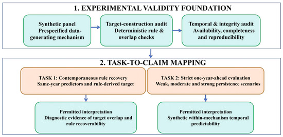
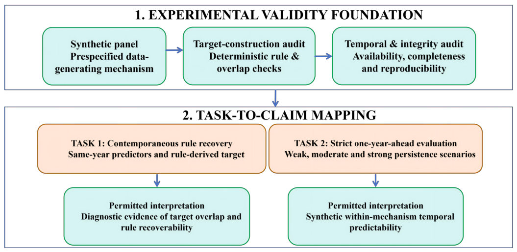
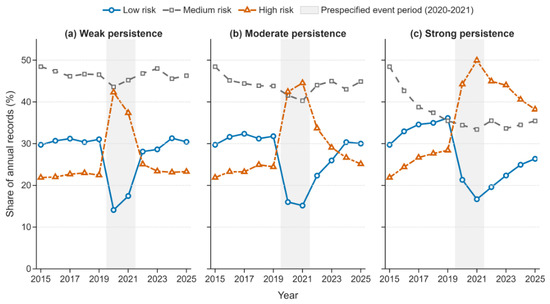
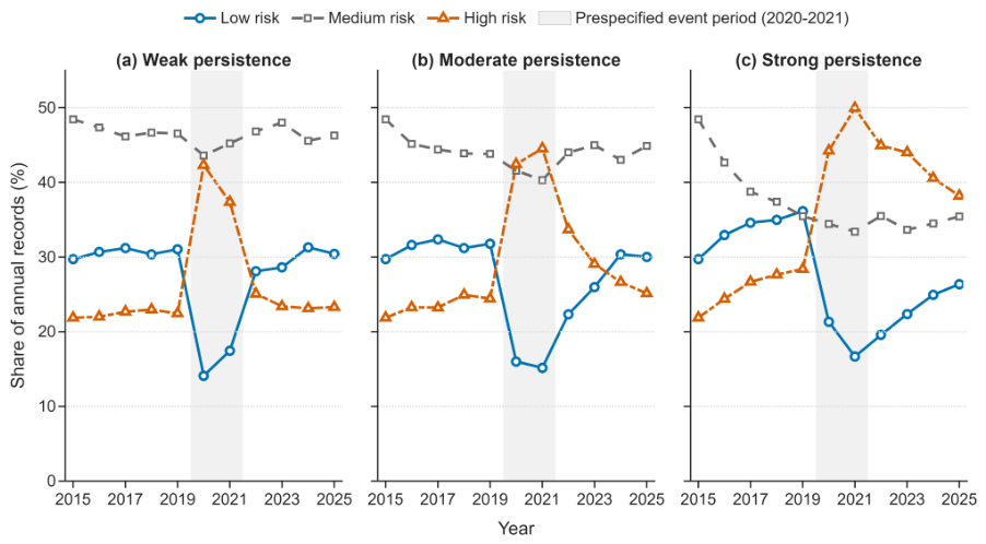
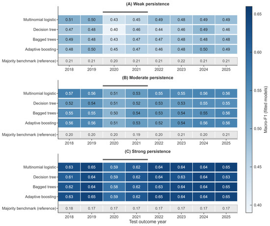
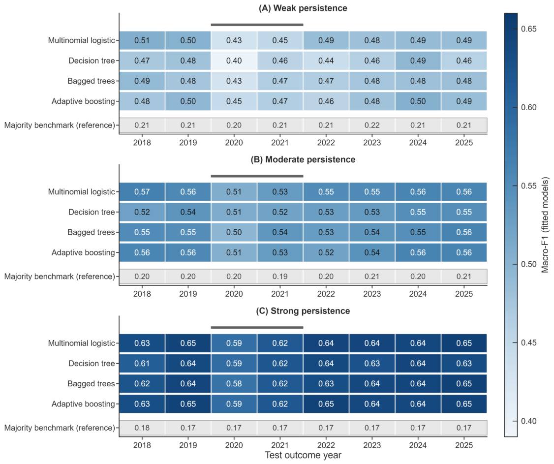
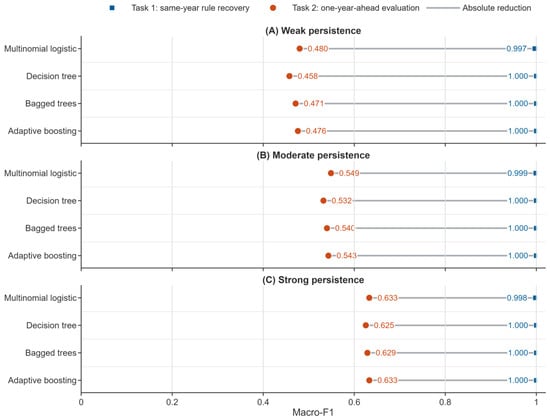
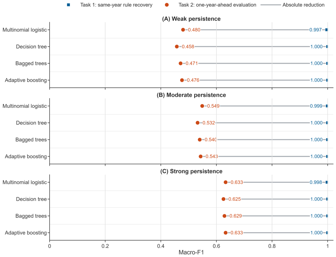

Disclaimer/Publisher’s Note: The statements, opinions and data contained in all publications are solely those of the individual author(s) and contributor(s) and not of MDPI and/or the editor(s). MDPI and/or the editor(s) disclaim responsibility for any injury to people or property resulting from any ideas, methods, instructions or products referred to in the content. |
© 2026 by the authors. Licensee MDPI, Basel, Switzerland. This article is an open access article distributed under the terms and conditions of the Creative Commons Attribution (CC BY) license.