


Highlights
What are the main findings?
- The COVID-19 shock in 2020 and the 2008 financial crisis emerged as the most influential extreme events affecting U.S. GDP and unemployment during the period examined.
- Machine-learning and hybrid forecasting approaches, especially Gradient Boosting and ensemble-based models, generally outperformed traditional time-series methods in capturing nonlinear extreme event effects.
What are the implications of the main findings?
- Forecasting models of economic disruption should incorporate crisis-sensitive bottleneck variables such as pandemic-related losses, industrial-sector disruption, DJIA movements, and federal interest-rate changes.
- Combining traditional time-series methods with flexible machine learning models can improve the forecasting of unstable macroeconomic behaviour during rare shocks.
Abstract
This paper contributes to the stream of literature on extreme event modelling and forecasting by comparing various forecasting methods for predicting extreme movements in GDP and unemployment in the United States. The data were obtained from multiple open sources for the USA, including CNBC, the U.S. National Library of Medicine, the National Institutes of Health, the Centres for Disease Control and Prevention, the Bureau of Transportation Statistics site, Investing Com, the U.S. Bureau of Labour Statistics, Yahoo Finance, The Balance and Wikipedia. The research focuses on identifying the optimal forecasting method between Machine Learning and time-series forecasting algorithms, for predicting extreme values of GDP and unemployment, accounting for natural disasters and industrial and economic factors. The statistical and analytical insights derived from this study, if used judiciously, can inform policymaking and planning.
1. Introduction
Research, to date, on the forecasting and economic impact of extreme events has been sparse and domain-specific. To that end, we contribute to this contemporary literature by applying machine learning and time-series methods to forecast extreme events affecting the USA. The contribution of this study to the forecasting literature is threefold. First, it offers a comparison between traditional time-series, machine learning, and hybrid forecasting methods in the context of macroeconomic extreme events. Second, it examines the outcomes using two main indicators, GDP and unemployment, which are at the centre of economic policy during periods of extreme disruption. Third, it combines calamity-related, industrial sector, economic, and combined datasets to identify crisis-sensitive variables that influence macroeconomic performance and recovery.
This research provides guidance for the duration of disruptions from different focal points and a rough indication of the recovery approach. As the well-known aphorism goes: “a failure to plan, is a plan to fail”; and thus, the “Raison d’être” for this research is to play a significant role in forecasting, planning and preparation for future extreme events. Indeed, these rare events cannot be accurately predicted, if at all; therefore, (responsible) governments should implement precautionary measures—in line with this analysis.
This paper is organised as follows: firstly, an in-depth literature review is discussed based on rare event forecasting, deep learning forecasting methods and historical epidemic/pandemic consequences, this gives an insight about the research gaps from past studies, helps in forming the research questions to be answered and gives an overview of how the research flow has to be carried out. Then, using a quantitative, broadly positivistic approach, secondary data from open sources are retrieved, cleaned, and pre-processed for analysis. This approach is appropriate as it examines observable macro indicators and assesses forecasting performance by using measurable statistics. However, we acknowledge that extreme events result from complex dynamics that cannot be captured fully by quantitative indicators alone.
Among several technical approaches, methods inspired by prior research and novel techniques are applied, and based on performance metrics, the best method is selected to forecast the revival period of the economy and the job market. This is followed by a discussion of the strengths, weaknesses, and prospects of this research.
In our work, preliminary empirical evidence suggests that, among several calamities in the past two decades, COVID-19 and the 2008 financial crisis have been the most influential events in affecting other economic and industrial factors, leading to the collapse of the economy and the job market. These economic and industrial factors can be considered as bottlenecks which can be further exploited as per the “Theory of Constraints”. In this paper, the “Theory of Constraints” is used only as a supporting conceptual lens.
2. The Pertinent Literature
In prior studies, quantitative models have demonstrated their ability to successfully extrapolate the primary trend-cycle of business and economic time series [1,2], but less so for an extreme event [3]—that is defined as a rare, unexpected occurrence that is beyond one’s imagination [4]. Several prior studies suggest that forecasters could rely on judgement, intuition, and experience to develop forecasts for extreme events [5]; nevertheless, with limited success [6].
In the past few decades, several studies have sought to develop efficient machine learning forecasting models. Lee and Yum [7] developed a framework to adjust the forecaster’s time-series judgments using an Artificial Neural Network (ANN). In another study using TV ratings data, Nikolopoulos et al. [8] concluded that ANN was slightly more efficient than the forecaster’s judgement, Multiple Linear Regression (MLR), and Nearest Neighbours methods. Nikolopoulos [9] evidenced that the EXPRT1 model (based on MLR) even with its superior result was less promising then the EXPRT2 model (based on ANN) because its performance supremacy might be due to the specific simulated data and the fact that EXPRT1 assumed that if R2 value is more than 95% or R2MLR is greater than R2ANN, the relationship between the features is linear. However, real-life data might be nonlinear.
Part of the problem is that data generated by natural phenomena are often chaotic and thus contain extreme values [10]. Nevertheless, few methods reliably generate models of chaotic time series, particularly for long-term predictions. To that end, in 2014, GenericPred was proposed by Golestani & Gras [11] using financial time series (Dow Jones Industrial Average), medical time series (Epileptic seizures) and climate time series (Global Historical Climatology Network Monthly and International Comprehensive Ocean–Atmosphere). For both short-term predictions (vs. Learning Financial Agent-Based Simulator (L-FABS), Multi-Layer Perceptron-MLP) as well as long-term ones (vs. ARIMA, GARCH, VAR), GenericPred was found to be more accurate. Buffa, Cosgrove and Lute [12] conducted a study to create a short-interval forecasting model of emergency phone calls (911) to estimate the workload on the operators, with Indianapolis Police Department (IPD) data using a Box–Jenkins univariate time-series approach. As with IPD, the banking industry also exhibits several characteristics, including demand patterns that are unevenly distributed over time, multiple cycles within a time series, and special events, such as holidays, that do not recur at regular intervals. To gain a better understanding of these parameters, six forecasting models were analysed: One Year Lag (OYL), Zero/One Regression (ZOR), multiplicative/additive (MA), ZORA with adjustment, MA with adjustment (MAA), and ARIMA. ZORA and MAA were found to perform better, with lower MAPE values, shorter processing times, and lower core requirements.
Service-based companies, such as Uber, rely heavily on an extreme event forecasting model for anomaly detection, optimal resource allocation, budget planning, and related tasks. Accurate prediction of rare events (e.g., holidays, sporting events) facilitates optimal driver allocation and thus reduces passenger waiting time. Most recent algorithms are based on the combination of a univariate forecasting method (e.g., Holt–Winters) and an ML method (e.g., Random Forest). However, these methods are laborious to incorporate external variables (e.g., weather, city population rates) and to scale and tune [13]. The past literature based on Long Short-Term Memory (LSTM) network—an artificial recurrent neural network [14]—shows that LSTM can incorporate exogenous variables, can do end-to-end modelling, can automatically extract the features, and can model complex nonlinear feature interactions [15].
However, in this case, a vanilla LSTM was unable to adapt to time-series data with a single neural network. Inspired by vanilla LSTM, Laptev, Yosinski, Li and Smyl [16] in Uber Technologies suggested an end-to-end Bayesian Neural network that generated both forecasting and estimation of the uncertainties. This model incorporated an Autoencoder for feature extraction, a prediction network to mitigate prediction uncertainty, and a Monte Carlo dropout framework to prevent changes in the neural network. Compared with the Naïve model, Quantile Random Forest (QRF), and LSTM, the Bayesian Deep model was found to be the most efficient, with nearly 95% uncertainty coverage.
Nonlinear autoregressive exogenous (NARX) models use nonlinear mapping to improve prediction [17]. However, their ability to learn from the input is limited by their shallow architecture [18]. To address these issues, considerable effort has been invested in studying deep neural networks (DNNs), as they enable better feature extraction. Among frameworks such as Boltzmann Machines [19], Convolutional Networks, and RNNs, RNNs appear to be a promising approach for time-series analysis. Based on this knowledge, Diaconescu [20] suggested combining an RNN with an NARX model to significantly reduce prediction errors. Due to the positive aspects of RNN, several amendments have been imposed on it to yield better results, such as Long-Short Term Memory and Gated Recurrent Unit (GRU). However, DNN models remain weak at forecasting due to their quadratic loss (based on Extreme Value Theory). To overcome this obstacle, Ding et al. [21], inspired by EVT, proposed the concept of Extreme Value Loss (EVL) to detect rare future events. In addition, they used a memory network framework to memorise the most extreme past data point. After extensive investigation of real stock and climate datasets, the proposed EVL-memory network was superior to competing models, including LSTM, Time-LSTM, GRU, and a memory network alone.
Makridakis, Spiliotis, and Assimakopoulos [22] respond to the literature advocating machine learning and deep learning models that promise higher accuracy than traditional models yet provide insufficient supporting evidence. The eight traditional time-series models used are as follows: Naive 2 (a random walk model adjusted for seasonality), Simple Exponential Smoothing (SES), Holt, Damped Exponential Smoothing, Average of SES-Holt-Damped, Theta method, ARIMA (automatic), and ETS (automatic). The ten ML methods used are as follows: Multi-Layer Perceptron (MLP), Bayesian Neural Network (BNN), Radial Basis Functions (RBFs), Generalised Regression Neural Networks (GRNN or kernel regression), K-Nearest Neighbour regression (KNN), CART regression trees (CART), Support Vector Regression (SVR), Gaussian Processes (GPs), Recurrent Neural Network (RNN), and Long Short-Term Memory (LSTM). Based on results from the M3 competition, MLP and BNN were the best-performing ML algorithms, whereas surprisingly, RNN and LSTM performed poorly. These methods have better model fitting but poor forecasting accuracy.
Nevertheless, based on results from the M3 competition, ETS and ARIMA were the best-performing methods overall for one-step forecasting, and Theta [2], ARIMA, and a combination of exponential smoothing (Comb) were the best-performing models in multi-step forecasting. However, based on more recent M4 competition it was found that a “hybrid model”, i.e., a combination of traditional time series methods and ML algorithm [23] was found to be 10% more accurate than Comb (used as a benchmark) as compared to the champion model of M3, that was 4% more accurate than Comb. This hybrid model was the integration of exponential smoothing and a “black box” RNN forecasting engine.
M-competitions are known for introducing novel and efficient forecasting models; however, the datasets used by them are not particularly complex. The suggested algorithms have not been tested on a dataset with missing information, complex structure, heavy noise, and complex interrelationships among variables. Also, Fildes and Makridakis [24] propose a forecasting model that combines and utilises the strengths of models suited to short- and long-term forecasting. The M1 competition [25] demonstrated that traditional methods were as accurate as, or more accurate than, sophisticated statistical methods. The M2 competition [26] showed that additional information and judgement had little effect on the accuracy of time-series forecasting. The M3 competition validated the results of M1 and introduced new, more accurate forecasting approaches. Finally, the M4 competition introduced a “hybrid” method, confirmed the superiority of an integrated model that included an ML framework to enhance accuracy, and introduced several powerful new methods for calculating KPIs. More recently, two more incarnations of these competitions, M5 and M6, provided the latest evidence on the empirical forecasting ‘horserace’ field [27,28].
Recent studies in this stream of literature directly connected to the predictability of extreme macroeconomic events have enhanced univariate forecasting, hybrid GDP forecasting, high-frequency macroeconomic indicators, GDP nowcasting, and probabilistic evaluation [29,30,31,32,33]. Similarly, evidence is supported and strengthened for examining crisis-related forecasting designs, including other macro indicators such as unemployment claims with online trends, big data, and nowcasting on COVID-19, interrupted time-series forecasting, and data-rich modelling of economic indicators [34,35,36,37,38].
Since 2020, due to the COVID-19 pandemic, numerous types of literature have emerged, and the work is still ongoing. To tackle the impact of the pandemic, several policies and amendments are proposed and stored in Baldwin and Weder di Mauro [39]. Economists have used accumulated data to study the relationship between pandemic incidence and its economic impacts, such as the impact of the 1918 Spanish flu, as analysed by Brainerd and Siegler [40], and more recently by Barro et al. [41]. However, most of the literature focuses on a single event in a single location. However, large-scale pandemics like COVID-19 affect all countries because of widespread transmission or interconnected trade and markets.
Most recent studies focus on short-term impacts due to mitigating circumstances [42]. Based on data from fifteen historical pandemics, including the Black Death, Jordà et al. [43] conducted a time-series analysis of the medium- to long-term impacts of COVID-19. This literature is inspired by the pandemic’s global macroeconomic ramifications, using historical data on pandemics in Europe. The economy centres on monetary policy, which largely depends on the real interest rate. This variable may affect the labour market, economic growth, and commodity prices. This literature concludes that the impact of pandemics can persist for several decades, with weakened investment opportunities. However, prior studies suggest that pandemics respond differently. For example, pandemics like Black Death and the Spanish flu resulted in the decline in the real interest rate due to the loss of labour without significant destruction of capital, whereas pandemics like wars result in elevated real interest rates for the next few decades due to the loss of labour along with the destruction of capital.
Barro and Ursúa [44] developed a regression model to estimate the impact of different pandemics on GDP. Based on this analysis, the three most severe events in terms of macroeconomic shocks worldwide after 1870 were World War II, the Great Depression (the early 1930s), and World War I, followed by the Spanish Flu. In one of the regression models, the two variables selected were GDP and personal consumer expenditure during the Great Influenza pandemic and World War I. It was found that Influenza reduced GDP by 6.2%, whereas war reduced it by 8.4% in affected countries. However, the model predicted potential growth in the years ahead. In another regression model, the two variables selected during the same period were stock returns and returns on short-term government bills. The results predicted that the market would recover after a short-term decline and that the net impact of war on returns would be negligible. Although both the Spanish flu and the war increased the inflation rate for some time. The more recent literature on the coronavirus pandemic [41] predicts a reduction in stock prices, increases in stock-price volatility, a decrease in nominal interest rates and 6% and 8% decline in GDP and private consumption, respectively, which is like the numbers seen during the global recession of 2008–2009. The depletion could be due to countries adopting policies to reduce real GDP, particularly in the travel and commerce sectors, to control the spread.
Non-pharmaceutical interventions (NPIs), such as social distancing and lockdowns, are the primary measures implemented during pandemics to reduce mortality. However, NPIs can also have a significant impact on the economy. Correia, Luck, and Verner [42] studied the effect of NPIs across the U.S. during the 1918 Spanish Flu period using an OLS difference-in-differences model. Based on the variation and intensity of NPIs, the economic impact was evaluated. In the short term, economic deprivation was similar across both firm and liberal NPI-imposed cities.
Although the implementation of NPIs led to unemployment and demand restrictions across many industries, especially manufacturing, in the medium term, evidence suggests that cities with stricter NPIs experienced a relative increase in economic activity by 1919. This is because stricter NPIs were associated with a lower mortality rate. However, several conditions vary in the case of the influenza pandemic as compared to COVID-19, such as the 1918 pandemic at the end of WWI, where the economy was already trembling, different economic policies were present, the female workforce was lower in 1918, a different cross-country trade framework was implemented, and there were no or limited options of work from home, etc. NPIs implemented in 2020 have reduced the spread of disease and thus prevented further significant economic downturn [45,46], and countries that implemented NPIs at earlier stages of the outbreak have shown relatively better short-term economic output [47].
Finally, a pertinent body of literature emerging in the post-COVID era concerns supply chain viability. Supply chain viability has emerged as a distinct area within operations research and management science during the COVID-19 pandemic [48]. The key idea was to represent and analyse a new quality of resilience, i.e., the ability of the supply chain to “maintain itself and survive in a changing environment through a redesign of structures and re-planning of performance with long-term impacts” [49]. Two recent special issues on supply chain viability in Omega [48] and IJPR [50], which together have published over 30 articles and received more than 100 submissions, have confirmed the growing interest in this area.
3. Methodology
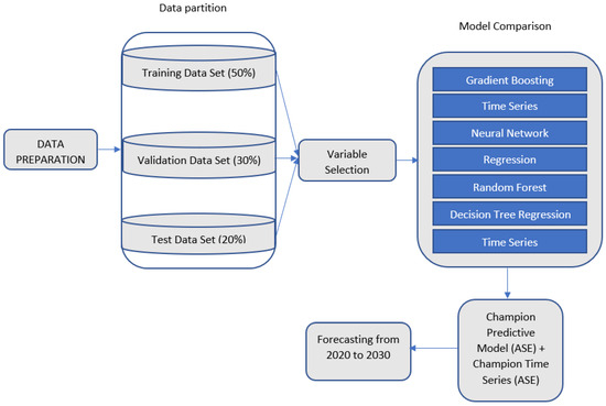
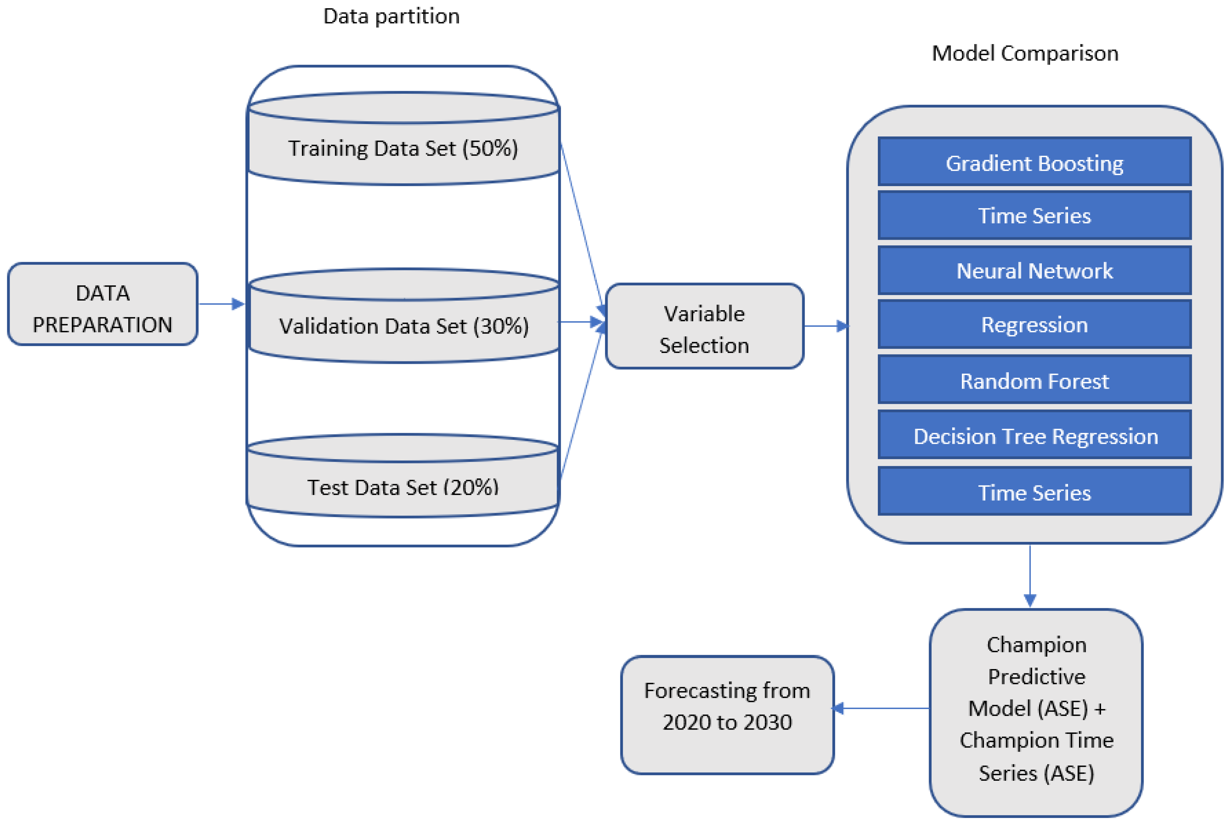
Our forecasting methodological flow is illustrated in Figure 1.
Figure 1.
Methodological workflow: data preparation, variable selection, model estimation, model comparison, and forecasting of GDP and unemployment under extreme event conditions.
After cleaning and preparing the data, variable selection is the next critical step to create the most robust model possible that fits the data effectively, thereby yielding more accurate predictions and more detailed interpretations. Since all datasets comprised rare events, the data could be linear or nonlinear. So, using SAS Enterprise Miner 15.3, several variable selection techniques (LARS, Decision Tree, variable clustering, variable selection) were applied, which would take both linear and nonlinear data into consideration, then combined with a regression node and compared against stepwise regression (specifically for linear data) via a model comparison node to find the best approach for variable selection. The surviving variables of this process, for calamities, industry, and economics, are presented in Table 1, Table 2 and Table 3, respectively. Nominal GDP is the dependent variable (target variable) in the “GDP model” while the total unemployment is the dependent variable (target variable for the “Unemployment-rate model”. Variables named “Selected predictor” were retained after the variable selection procedure. The variables labelled “Not selected” were excluded from the final model specification.
Table 1.
Calamity variables.
Table 2.
Industry variables.
Table 3.
Economics variables.
Prior to modelling, the data were cleaned, checked, and arranged into a common time-series structure. Since the variables were collected from different secondary sources and reported in different formats, they were converted into a consistent frequency to make comparisons possible across datasets. Missing observations were examined and treated depending on the variable and the extent of missing data. The cleaning process included checking the consistency of units, removing duplicate observations, correcting clear coding errors, and standardising date formats. Where appropriate, variables were normalised to make indicators with different scales more comparable within the modelling framework.
4. Results and Discussions
We ran seven (7) different types of forecasting methods: Neural Network (MLP, GLM, ORBFUN, ORBFEQ), Decision Tree (Decision Tree Regression), Regression (Linear regression), Random Forest, Gradient Boosting, ensemble (MLP, GLM, ORBFUN, ORBFEQ, Gradient Boosting, Decision Tree, Regression) and time series (VAR, Exponential Smoothing). We used the Average Squared Error (ASE) as the error metric to measure performance. The results are presented in Table 4.
Table 4.
Comparative performance of forecasting methods.
Table 5 highlights all the extreme events detected. It is evident that 2008 and 2020 were extreme events; hence, they can be termed crucial rare events that affected U.S. GDP and the unemployment rate the most. Thus, the Financial Crisis of 2008 and the Financial Crisis of 2020, caused by COVID-19 and by COVID-19 itself, have taken the greatest toll in terms of GDP decline and unemployment increase over the past two decades.
Table 5.
Outliers/rare events detected.
Changes reported in Table 5 represent a relative percentage change from the relevant previous reference value, rather than percentage point changes in the reported macroeconomic statistic.
5. Conclusions and the Future Directions
Based on analyses of all datasets, the most impactful calamity was the 2020 coronavirus outbreak, which resulted in a steep decline in GDP and a sharp rise in the unemployment rate, followed by the 2008 financial crisis. In this research, different focal points were used to forecast GDP and unemployment rate. Thus, this research has a broad spectrum for analysis. The secondary data for this study were obtained from multiple sources to create four datasets based on calamity, industrial sectors, economic indicators, and combo (industrial + economic). Due to rare, random events over the past two decades, the data are noisy and do not exhibit any discernible trend.
For the calamity, a statistical analysis was performed to find the contribution of each selected variable to the GDP. Epidemic/pandemic damage to infrastructure and other assets affected GDP most, particularly in 2020. Using the forecasting model (Gradient Boosting + ES), rare events were shortlisted in the outlier table, and the model forecasts that GDP will re-stabilise by March 2029.
For industrial, with GDP as the target, the rise of the pharmaceutical industry (AstraZeneca) impacted GDP the most (positively) during the pandemic period. Using the forecasting model (ensemble + ES), rare events were shortlisted in the outlier table, and the model forecasts that GDP will re-stabilise by May 2021. With the unemployment rate as the target, the automotive industry’s financial losses from probable supply chain restrictions during lockdowns adversely affected the job market. In the forecasting model (ORBFUN + ES), rare events were shortlisted in the outlier table, and the model was inefficient at representing the true unemployment forecast.
From an economic perspective, with GDP as the target, a decline in the DJIA closing value played a crucial role in the decline in GDP. Using the forecasting model (Gradient Boosting + ES), rare events were shortlisted in the outlier table, and the model forecasts that GDP will re-stabilise by February 2026. Given that the unemployment rate is the primary target, the reduction in the federal funds rate during the 2020 COVID-19 pandemic and the 2009 financial crisis is associated with a deteriorating labour market. Using the forecasting model (Gradient Boosting + ES), rare events were shortlisted in the outlier table, and the model forecasts that the unemployment rate will return to normal by September 2022.
For combo, with GDP as the target, the DJIA closing value has the greatest effect on GDP. Using the forecasting model (Gradient Boosting + ES), rare events were shortlisted in the outlier table, and the model forecasts that GDP will re-stabilise by November 2024. Given that the unemployment rate is the target, financial losses in the automotive or manufacturing industry may lead to unemployment. In the forecasting model (ORBFUN + ES), rare events were shortlisted in the outlier table, and the forecast reached saturation; hence, it was inefficient at predicting the re-stabilisation period for unemployment.
Predictors such as epidemic/pandemic damage cost, pharmaceutical industry, automotive industry, DJIA closing value and Federal interest rate can be termed as the bottlenecks as per their relationship with the economy as GDP and unemployment rate depends on these factors the most, and by the “Theory of Constraints”, these bottlenecks can be exploited the most as an attempt to boost the economy during the ongoing pandemic.
Author Contributions
Conceptualization, R.S., K.N., A.A. and V.B.; methodology, K.N. and R.S.; software, A.A. and R.S.; validation, K.N. and V.B.; formal analysis, R.S. and A.A.; investigation, R.S., A.A., V.B. and K.N.; data curation, R.S.; writing-original draft preparation, R.S.; writing-review and editing, K.N. and V.B.; visualization, R.S., supervision, K.N.; project administration, K.N. All authors have read and agreed to the published version of the manuscript.
Funding
This research received no external funding.
Data Availability Statement
Data are available upon request from R. Shankar.
Conflicts of Interest
The authors declare no conflict of interest.
References
- Makridakis, S.; Hibon, M. The M3-Competition: Results, conclusions and implications. Int. J. Forecast. 2000, 16, 451–476. [Google Scholar] [CrossRef] [Scilit]
- Assimakopoulos, V.; Nikolopoulos, K. The theta model: A decomposition approach to forecasting. Int. J. Forecast. 2000, 16, 521–530. [Google Scholar] [CrossRef] [Scilit]
- Nikolopoulos, K.; Bougioukos, N.; Giannelos, K.; Assimakopoulos, V. Estimating the impact of shocks with artificial neural networks. In Artificial Neural Networks—ICANN 2007; Lecture Notes in Computer Science; Springer: Berlin/Heidelberg, Germany, 2007; Volume 4669, pp. 476–485. [Google Scholar]
- Taleb, N.N. The Black Swan: The Impact of the Highly Improbable; Random House: New York, NY, USA, 2007. [Google Scholar]
- Armstrong, J.S. Principles of Forecasting: A Handbook for Researchers and Practitioners; Kluwer Academic Publishers: Boston, MA, USA, 2001. [Google Scholar]
- Goodwin, P. Integrating management judgment and statistical methods to improve short-term forecasts. Omega 2002, 30, 127–135. [Google Scholar] [CrossRef] [Scilit]
- Lee, J.K.; Yum, B.J. Judgmental adjustment in time series forecasting using neural networks. Decis. Support Syst. 1998, 22, 135–154. [Google Scholar] [CrossRef] [Scilit]
- Nikolopoulos, K.; Goodwin, P.; Patelis, A.; Assimakopoulos, V. Forecasting with cue information: A comparison of multiple regression with alternative forecasting approaches. Eur. J. Oper. Res. 2007, 180, 354–368. [Google Scholar] [CrossRef] [Scilit]
- Nikolopoulos, K. Forecasting with quantitative methods: The impact of special events in time series. Appl. Econ. 2010, 42, 947–955. [Google Scholar] [CrossRef] [Scilit]
- Romanelli, L.; Figliola, M.A.; Hirsch, F.A. Deterministic chaos and natural phenomena. J. Stat. Phys. 1988, 53, 991–994. [Google Scholar] [CrossRef] [Scilit]
- Golestani, A.; Gras, R. Can we predict the unpredictable? Sci. Rep. 2014, 4, 6834. [Google Scholar] [CrossRef] [Scilit] [PubMed]
- Buffa, E.S.; Cosgrove, M.J.; Luce, B.J. An integrated work shift scheduling system. Decis. Sci. 1976, 7, 620–630. [Google Scholar] [CrossRef] [Scilit]
- Horne, J.; Manzenreiter, W. Football Goes East: Business, Culture and the People’s Game in China, Japan and South Korea; Routledge: London, UK, 2004. [Google Scholar]
- Hochreiter, S.; Schmidhuber, J. Long short-term memory. Neural Comput. 1997, 9, 1735–1780. [Google Scholar] [CrossRef] [Scilit]
- Assaad, M.; Boné, R.; Cardot, H. A new boosting algorithm for improved time-series forecasting with recurrent neural networks. Inf. Fusion 2008, 9, 41–55. [Google Scholar] [CrossRef] [Scilit]
- Laptev, N.; Yosinski, J.; Li, L.E.; Smyl, S. Time-series extreme event forecasting at scale. In Proceedings of the International Conference on Machine Learning, Sydney, Australia, 6–11 August 2017; pp. 1–5. [Google Scholar]
- Lin, T.; Horne, B.G.; Tino, P.; Giles, C.L. Learning long-term dependencies in NARX recurrent neural networks. IEEE Trans. Neural Netw. 1996, 7, 1329–1338. [Google Scholar]
- Bengio, Y.; Lamblin, P.; Popovici, D.; Larochelle, H. Greedy layer-wise training of deep networks. In Advances in Neural Information Processing Systems 19; MIT Press: Cambridge, MA, USA, 2006. [Google Scholar]
- Dasgupta, S.; Osogami, T. Nonlinear dynamic Boltzmann machines for time-series prediction. In Proceedings of the Thirty-First AAAI Conference on Artificial Intelligence, San Francisco, CA, USA, 4–9 February 2017; pp. 1833–1839. [Google Scholar]
- Diaconescu, E. The use of NARX neural networks to predict chaotic time series. WSEAS Trans. Comput. Res. 2008, 3, 182–191. [Google Scholar]
- Ding, D.; Zhang, M.; Pan, X.; Yang, M.; He, X. Modeling extreme events in time series prediction. In Proceedings of the 25th ACM SIGKDD International Conference on Knowledge Discovery & Data Mining, Anchorage, AK, USA, 4–8 August 2019; pp. 1114–1122. [Google Scholar]
- Makridakis, S.; Spiliotis, E.; Assimakopoulos, V. Statistical and machine learning forecasting methods: Concerns and ways forward. PLoS ONE 2018, 13, e0194889. [Google Scholar] [CrossRef] [Scilit] [PubMed]
- Smyl, S. A hybrid method of exponential smoothing and recurrent neural networks for time series forecasting. Int. J. Forecast. 2020, 36, 75–85. [Google Scholar] [CrossRef] [Scilit]
- Fildes, R.; Makridakis, S. The impact of empirical accuracy studies on time series analysis and forecasting. Int. Stat. Rev. 1995, 63, 289–308. [Google Scholar] [CrossRef] [Scilit]
- Makridakis, S.; Andersen, A.; Carbone, R.; Fildes, R.; Hibon, M.; Lewandowski, R.; Newton, J.; Parzen, E.; Winkler, R. The accuracy of extrapolation/time series methods: Results of a forecasting competition. J. Forecast. 1982, 1, 111–153. [Google Scholar] [CrossRef] [Scilit]
- Makridakis, S.; Chatfield, C.; Hibon, M.; Lawrence, M.; Mills, T.; Ord, K.; Simmons, L.F. The M2-Competition: A re-al-time judgementally based forecasting study. Int. J. Forecast. 1993, 9, 5–22. [Google Scholar] [CrossRef] [Scilit]
- Makridakis, S.; Petropoulos, F.; Spiliotis, E. The M5 competition: Conclusions. Int. J. Forecast. 2022, 38, 1576–1582. [Google Scholar] [CrossRef] [Scilit]
- Makridakis, S.; Spiliotis, E.; Hollyman, R.; Petropoulos, F.; Swanson, N.; Gaba, A. The M6 forecasting competition: Bridging the gap between forecasting and investment decisions. Int. J. Forecast. 2025, 41, 1315–1354. [Google Scholar] [CrossRef] [Scilit]
- Petropoulos, F.; Spiliotis, E. The wisdom of the data: Getting the most out of univariate time series forecasting. Forecasting 2021, 3, 478–497. [Google Scholar] [CrossRef] [Scilit]
- Chapman, J.T.; Desai, A. Macroeconomic predictions using payments data and machine learning. Forecasting 2023, 5, 652–683. [Google Scholar] [CrossRef] [Scilit]
- Le Gal La Salle, J.; David, M.; Lauret, P. A set of new tools to measure the effective value of probabilistic forecasts of continuous variables. Forecasting 2025, 7, 30. [Google Scholar] [CrossRef] [Scilit]
- Assunção, J.B.; Fernandes, P.A. Nowcasting GDP: An application to Portugal. Forecasting 2022, 4, 717–731. [Google Scholar] [CrossRef] [Scilit]
- Tampouris, A.; Dritsaki, C. GDP forecasting with ARIMA, hidden Markov models, and an HMM–LSTM hybrid: Evidence from five economies. Forecasting 2026, 8, 30. [Google Scholar] [CrossRef] [Scilit]
- Aaronson, D.; Brave, S.A.; Butters, R.A.; Fogarty, M.; Sacks, D.W.; Seo, B. Forecasting unemployment insurance claims in realtime with Google Trends. Int. J. Forecast. 2022, 38, 567–581. [Google Scholar] [CrossRef] [Scilit]
- Barbaglia, L.; Frattarolo, L.; Onorante, L.; Pericoli, F.M.; Ratto, M.; Pezzoli, L.T. Testing big data in a big crisis: Nowcasting under COVID-19. Int. J. Forecast. 2023, 39, 1548–1563. [Google Scholar] [CrossRef] [Scilit]
- Hyndman, R.J.; Rostami-Tabar, B. Forecasting interrupted time series. J. Oper. Res. Soc. 2025, 76, 790–803. [Google Scholar] [CrossRef] [Scilit]
- Kynigakis, I.; Panopoulou, E. Modeling the distribution of key economic indicators in a data-rich environment: New empirical evidence. J. Oper. Res. Soc. 2025, 76, 2071–2090. [Google Scholar] [CrossRef] [Scilit]
- Kourentzes, N.; Svetunkov, I. Incorporating risk preferences in forecast selection. J. Oper. Res. Soc. 2026, 1–16. [Google Scholar] [CrossRef] [Scilit]
- Baldwin, R.; di Mauro, B.W. (Eds.) Economics in the Time of COVID-19; Centre for Economic Policy Research: London, UK, 2020. [Google Scholar]
- Brainerd, E.; Siegler, M.V. The Economic Effects of the 1918 Influenza Epidemic; CEPR Discussion Paper No. 3791; Centre for Economic Policy Research: London, UK, 2003. [Google Scholar]
- Barro, R.J.; Ursúa, J.F.; Weng, J. The Coronavirus and the Great Influenza Pandemic: Lessons from the “Spanish Flu” for the Coronavirus’s Potential Effects on Mortality and Economic Activity; NBER Working Paper No. 26866; National Bureau of Economic Research: Cambridge, MA, USA, 2020. [Google Scholar]
- Correia, S.; Luck, S.; Verner, E. Pandemics depress the economy, public health interventions do not: Evidence from the 1918 flu. J. Econ. Hist. 2022, 82, 917–957. [Google Scholar] [CrossRef] [Scilit]
- Jordà, Ò.; Singh, S.R.; Taylor, A.M. Longer-run economic consequences of pandemics. Rev. Econ. Stat. 2022, 104, 166–175. [Google Scholar] [CrossRef] [Scilit]
- Barro, R.J.; Ursúa, J.F. Macroeconomic crises since 1870. Brook. Pap. Econ. Act. 2008, 2008, 255–350. [Google Scholar] [CrossRef] [Scilit]
- Andersen, A.L.; Hansen, E.T.; Johannesen, N.; Sheridan, A. Consumer responses to the COVID-19 crisis: Evidence from bank account transaction data. Scand. J. Econ. 2022, 124, 905–929. [Google Scholar] [CrossRef] [Scilit]
- Lin, Z.; Meissner, C.M. Health vs. Wealth? Public Health Policies and the Economy During COVID-19; NBER Working Paper No. 27099; National Bureau of Economic Research: Cambridge, MA, USA, 2020. [Google Scholar]
- Demirgüç-Kunt, A.; Pedraza, A.; Ruiz-Ortega, C. Banking Sector Performance During the COVID-19 Crisis; World Bank Policy Research Working Paper No. 9363; World Bank: Washington, DC, USA, 2020. [Google Scholar]
- Ivanov, D.; Keskin, B.B. Post-pandemic adaptation and development of supply chain viability theory. Omega 2023, 116, 102806. [Google Scholar] [CrossRef] [Scilit]
- Ivanov, D. Correction to: Viable supply chain model: Integrating agility, resilience and sustainability perspectives—Lessons from and thinking beyond the COVID-19 pandemic. Ann. Oper. Res. 2022, 319, 1411–1431. [Google Scholar] [CrossRef] [Scilit] [PubMed]
- Ivanov, D.; Dolgui, A.; Blackhurst, J.V.; Choi, T.M. Toward supply chain viability theory: From lessons learned through COVID-19 pandemic to viable ecosystems. Int. J. Prod. Res. 2023, 61, 2402–2415. [Google Scholar] [CrossRef] [Scilit]

Disclaimer/Publisher’s Note: The statements, opinions and data contained in all publications are solely those of the individual author(s) and contributor(s) and not of MDPI and/or the editor(s). MDPI and/or the editor(s) disclaim responsibility for any injury to people or property resulting from any ideas, methods, instructions or products referred to in the content. |
© 2026 by the authors. Licensee MDPI, Basel, Switzerland. This article is an open access article distributed under the terms and conditions of the Creative Commons Attribution (CC BY) license.