


Highlights
What are the main findings?
- The accuracy of the developed wind speed forecasting model based on a Gaussian process (GP) for residual modelling largely depends on the local wind regime.
- The GP model improved forecast accuracy by up to 16.3% at high-elevation inland stations. In contrast, the model was ineffective at the low-elevation coastal stations.
What are the implications of the main findings?
- The success of sophisticated residual modelling techniques, including the Gaussian process model, cannot be generalised and should be adapted to particular geographical and meteorological regimes.
- The forecasting process should account for the clustering of monitoring stations by geographical location and elevation, e.g., inland or coastal areas.
Abstract
Accurate wind speed forecasting is essential for the efficient integration of wind energy into power systems, as it directly influences generation scheduling, grid stability, and energy market operations. Forecast errors can lead to significant economic losses, including increased balancing costs, inefficient dispatch of backup generation, and penalties in electricity markets. However, wind behaviour is highly complex due to the influence of synoptic weather systems, terrain variability, and turbulence, which makes accurate prediction particularly challenging. This paper proposes a hybrid modelling framework that combines a linear regression mean model with Gaussian process (GP) residual modelling to improve forecast accuracy. Monitoring stations were grouped based on geographic coordinates and elevation, with cluster validation using the Hopkins statistic and silhouette analysis. The results show that for high-elevation inland stations (cluster 2), GP residual modelling improves forecast accuracy by up to 16.3%. In contrast, for low-elevation coastal stations (cluster 1), the GP approach does not yield improvements, indicating that its effectiveness depends strongly on the underlying wind regime.
1. Introduction
1.1. Overview
Wind speed forecasting plays a critical role in the integration of wind energy into modern power systems, particularly as countries transition towards low-carbon energy sources. Accurate forecasts are essential for generation scheduling, grid stability, and participation in electricity markets. Forecast errors can have significant economic and operational consequences: overestimation of wind power may lead to unnecessary curtailment and financial penalties, while underestimation can result in reliance on costly backup generation and increased balancing costs. Furthermore, the inherent variability and intermittency of wind pose substantial challenges for grid integration, requiring system operators to manage uncertainty across multiple spatial and temporal scales. Despite its importance, wind behaviour remains difficult to model due to its complex, intermittent spatial and temporal dynamics, which are influenced by atmospheric conditions, topography, and local turbulence. Linear models are often effective in capturing large-scale trends but fail to account for localised dependencies, while purely data-driven approaches may achieve high predictive accuracy at the expense of interpretability and uncertainty quantification.
The use of GPs is advantageous for spatio-temporal forecasting because the method is probabilistic, allowing for uncertainty and covariance to be explicitly incorporated into the modelling process. But GPs have limitations: they are computationally intensive when applied to large datasets, and they may become redundant when applied to raw wind speed measurements. The proposed alternative here is to use GPs in the residual part of a mean model. There are also issues of variability across different wind regimes by geographic location; there is a significant difference in wind characteristics between low-elevation coastal areas and high-elevation inland areas. It would negatively affect forecast performance if the spatial heterogeneity of the wind regime was not taken into account. The current study, therefore, suggests using a combined approach combining linear regression and Gaussian process models for residual analysis.
1.2. Literature Review
Accurate forecasting of wind speeds is critical for integrating wind energy into the grid and for various meteorological needs. Unfortunately, the chaotic behaviour of wind, influenced by large-scale atmospheric conditions, local topography, and turbulence, makes wind speed forecasting a complex problem. This review traces the chronological and thematic developments of wind speed forecasting techniques, from earlier physical and statistical models to modern hybrid and probabilistic models. It focuses on the developments of Gaussian process regression (GPR) and the utilisation of clustering techniques, both of which are significant to the proposed research. A brief overview of the major models is presented in Table 1.
Table 1.
Comparison of wind speed forecasting methods.
1.2.1. Classical Methods: Physical and Statistical Models
Traditionally, wind speed forecasting was carried out using Numerical Weather Prediction (NWP) models, which simulate atmospheric physics to predict wind speeds. These are certainly essential in wind speed forecasting; however, these models are subject to systematic errors and lack spatial resolution, which are often overcome by post-processing these results to increase their accuracy locally [1]. To overcome these problems, statistical time-series models such as ARIMA and SARIMA were widely applied. These models are effective in capturing linear trends and seasonality in wind speeds; however, they are not effective in capturing rapid, nonlinear changes in wind speeds, which are characteristic of wind speeds in general [2]. More adaptive models, such as Kalman Filters, were then applied to correct errors in short-term forecasts; however, these filters rely on linear assumptions and are prone to noise, limiting their application to wind speed forecasting over longer time scales and in spatially heterogeneous domains [3].
1.2.2. The Ascent of Machine Learning and Deep Learning
The limitations of linear models triggered the development and application of machine learning (ML) and deep learning (DL) techniques. ML and DL models, including random forests, Convolutional Neural Networks (CNNs), and Long Short-Term Memory (LSTM), are very effective at learning complex, nonlinear relationships directly from historical data, often resulting in significant accuracy gains in forecasts [4]. The hybrid model, combining NWP model results and LSTM, is also very effective for forecasting complex terrain, including nonlinear relationships and temporal dependencies [5]. However, ML/DL-based models are computationally intensive, require careful tuning, and often struggle to generalise across different locations. Additionally, ML/DL models are considered “black box” models, which limits their interpretability, making interpretability a driving need for finding models that are effective yet transparent and physically plausible [4,5].
1.2.3. Probabilistic Forecasting and Gaussian Process Regression
As the need to quantify uncertainty in grid operations increases, probabilistic forecasting has become a crucial area of study. Unlike point forecasts, probabilistic forecasting can offer predictive distributions for better risk-informed decision-making [6]. Bayesian methods, including Bayesian neural networks and Bayesian-Optimised models, inherently offer uncertainty quantification. However, their site-specific calibration can be a hindrance for real-time applications [7].
Within this paradigm, Gaussian process regression (GPR) has emerged as a prominent nonparametric tool for probabilistic forecasting. GPR is particularly prized for its capacity to yield a mean estimate and a well-founded interval estimate, which capture the essential randomness of wind phenomena [8]. The efficacy of GPR is critically dependent on its covariance function (kernel), which embodies assumptions regarding the underlying process, e.g., smoothness, periodicity, etc. GPR has been successfully utilised in hybrid frameworks, e.g., coupling GPR with support vector regression to post-process NWP forecasts for short-term forecasting (1 to 6 h ahead) [9]. Another hybrid model, which is a focus of this research, is a linear mean model coupled with a GPR model for forecasting residuals. This model balances interpretability with the power of GPR for modelling complex, spatially correlated error structures. However, standard GPR is known to scale poorly to large datasets, requiring a cubic time complexity () for its implementation [9,10].
1.2.4. Spatio-Temporal Modelling and the Role of Clustering
The spatial correlations in wind fields suggest that using data from adjacent areas can improve local predictions. A more advanced version of GPR, known as kriging, which is analogous to geostatistics, has been employed to interpolate wind fields while accounting for spatial correlations. It provides predictions along with their uncertainties [9]. More recent models seek to address complex spatio-temporal interactions. For example, dynamic versions of GPR that incorporate local clustering for improving accuracy have been presented [11]. Bayesian models for spatio-temporal forecasting for renewable energy forecasting have also been presented, but their success relies on the availability of dense data [12].
A notable result of the recent research is the recognition that wind speed statistical properties are not necessarily homogeneous over vast geographical areas. Various regimes, depending on the presence or absence of factors such as coastal areas and altitude, exhibit unique properties, including levels of non-stationarity, turbulence, and autocorrelation. This means that rather than seeking an optimal model applicable over the global domain, the regime-based approach of dividing the domain into homogeneous areas is more advisable. Grouping stations by their physical properties, such as geographic coordinates and altitude, is a statistically sound approach for dividing the domain.
Recent research emphasizes the potential of using the latest GP variants. For example, the application of hybrid GP approaches, which integrate spatial correlation with corrected NWP forecast information, has been found to offer better accuracy than the standard GP model [13]. Another GP model variant, the multi-task GP, is also found to be beneficial, particularly when applied to data-scarce locations, where information from data-rich locations can be exploited [14]. However, the current GP model variants, including the complex residual model, have the limitation that their added value is assumed to be applicable uniformly across the study area.
1.3. Summary of Literature Review
This research addresses the limitation of the complex residual model directly by proposing a hybrid linear-GP model, not over the entire study area but over geographically and elevation-based clusters. This is to evaluate the added value of the complex residual model across regimes, providing a physically informed, computationally efficient tool to improve the accuracy of wind speed forecasts.
A summary of the comparison of wind speed forecasting methods, including the key studies discussed, highlighting their temporal focus, uncertainty quantification, computational cost and limitations, is given in Table 1.
Despite significant advances in wind speed prediction techniques, several critical shortcomings remain. Traditional statistical models have drawbacks associated with their linear nature and their inability to incorporate more complex spatial relationships. Although machine learning and deep learning algorithms improve accuracy, they are not always interpretable and cannot provide proper uncertainty estimates. In turn, Gaussian processes solve both problems; however, they are computationally expensive. Finally, although hybrid and spatio-temporal models can offer more accurate predictions, they implicitly assume that improvements in model performance can be applied universally, regardless of local conditions such as terrain height and proximity to the coast. As a result, no algorithms can deliver high performance across interpretability, computation time, uncertainty estimation, and spatial heterogeneity. This gap motivates the proposed hybrid framework, which combines a linear mean model with Gaussian process residual modelling while explicitly incorporating regime-based clustering to account for spatial variability in wind behaviour.
1.4. Contribution and Research Highlights
The main contribution of the study under discussion is to demonstrate that hybrid models of linear and Gaussian processes for wind speed prediction must be used selectively, depending on the wind regime. Using clustering of elevations and coordinates, it is established that the Gaussian process residuals can be highly beneficial in high-variability areas (with up to 16.3% RMSE improvement) but potentially harmful in homogeneous clusters.
The main research highlights of this study are as follows:
- The hybrid linear–Gaussian process model considers the wind speed as a sum of two components, namely, the linear mean and GP residual, ensuring both clarity and spatial interactions between locations.
- Cluster analysis based on geographic coordinates and elevation allows for location-dependent analysis of the wind speed.
- The probabilistic nature of the GP component gives information about predictive uncertainty, making risk-based decisions possible for wind energy management.
- Systematic selection and optimisation of hyperparameters ensure capturing of spatial and temporal interaction in the wind regime.
- The study shows strong dependence of GP residual modelling effectiveness on wind regime.
The rest of the paper is organised as follows. Section 2 briefly discusses materials and methods, including the Hopkins variable selection method, temporal GP regression, linear temporal regression, the hybrid, and the evaluation metrics. Section 4 presents the results, the discussion is presented in Section 5, and the conclusion is in Section 6.
2. Materials and Methods
- Flowchart of the process
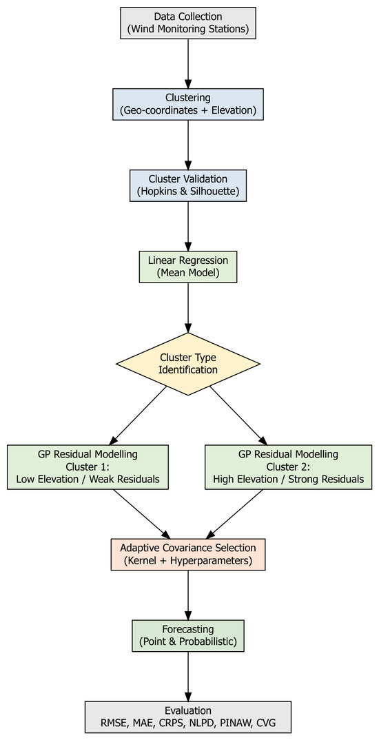
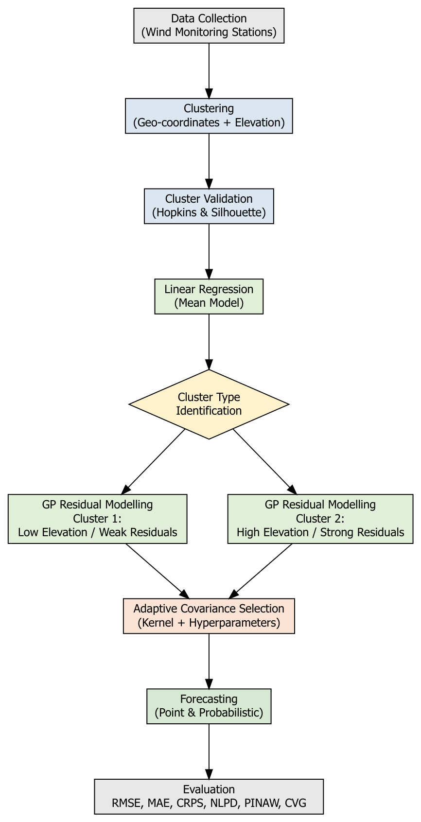
Figure 1 shows the flowchart of the structure of the paper. The process starts with collecting the required data from wind sensors, after which clustering is performed based on geo-coordinates and altitude. Cluster quality is assessed using the Hopkins and Silhouette measures. Clusters are created based on altitude and residual magnitude. Each type of residual model (low- and high-altitude) uses a Gaussian Process (GP) model with adaptive covariance selection.
Figure 1.
Flowchart of the structure of the paper.
Data Description and Clustering
The data used in this study are from the Wind Atlas South Africa (WASA) at https://wasadata.csir.co.za/wasa1/WASAData?pscreen=nwa&pemail=nimo@risoe.dtu.dk (accessed on 16 January 2025). The WASA data was obtained from the website [15]. Wind speed data from 10 stations were collected, each with multiple meteorological predictors (e.g., temperature and pressure). The variables included are as follows: Wind speed (m/s) at hub height (62 m). The data also feature the temporal aspect, which is the time of the day; the spatial aspect, which is the coordinates; and the meteorological aspect, which includes temperature, barometric pressure, relative humidity, and wind direction. These measurements were recorded every 10 min for all variables.
- Clustering
Wind conditions in several neighbouring wind farms are likely similar to each other because they are subject to similar weather conditions. To reduce computation, several wind farms can be combined into clusters, enabling forecasts based on clusters rather than individual wind farms. There is an advantage to combining information from several wind farms in the cluster, as it may help iron out local weather extremes.
To capture regime-dependent wind dynamics, stations were clustered using geographical coordinates (longitude and latitude) and elevation. We first used the Hopkins test to assess the dataset’s tendency to form clusters and determine whether the data are meaningfully clustered or randomly distributed (i.e., not clusterable). According to the method proposed by Hopkins and Skellam [16], the clustering tendency can be quantified using the Hopkins statistic H defined as
where suggests strong evidence of the cluster structure, while suggests little or no cluster tendency. Thereafter, we used hierarchical clustering to group the data. This is a method of cluster analysis that builds a hierarchy of clusters to uncover the underlying structure in a dataset. It does not rely on probability distributions, making it a nonparametric method, suitable even when the underlying data distribution is unknown. It also produces a dendrogram, a tree diagram, that provides a visual, flexible representation of how clusters form at different levels. This allows for users to choose the number of clusters by cutting the tree at the desired level.
- Variable selection—Relaxed Lasso
The Relaxed Lasso is a two-stage modification of the standard Lasso regression that aims to reduce the bias introduced by Lasso’s shrinkage, particularly in high-dimensional settings [17]. Lasso performs both variable selection and shrinkage by minimising Equation (2): Lasso estimates regression coefficients by solving Equation (2). As shown in Equation (2), the Lasso introduces an -penalty to enforce sparsity.
where is the response vector, is the predictor matrix, and is the vector of regression coefficients. The notation denotes the -norm (Euclidean norm), and denotes the -norm, defined as the sum of absolute values of the vector components. The regularisation parameter controls the trade-off between model fit and sparsity.
The factor expresses the loss as average empirical risk; alternative scalings (e.g., ) are equivalent up to a rescaling of the tuning parameter . While effective for variable selection, the Lasso tends to over-shrink coefficient estimates, leading to biased results.
where is the Lasso solution at regularisation level , and is the ordinary least squares estimator computed on the subset of variables selected by the Lasso. The parameter is a relaxation parameter controlling the degree of shrinkage. When , the estimator reduces to the standard Lasso; when , it corresponds to unregularised least squares on the Lasso-selected model. Intermediate values of provide a bias–variance trade-off.
The Relaxed Lasso addresses the tendency of the Lasso to over-shrink coefficients by decoupling variable selection and coefficient estimation. Specifically, it first performs variable selection using the Lasso and then refits the model with reduced shrinkage on the selected variables, improving estimation accuracy.
3. Methodology
3.1. GPR Models for Wind Forecasting
Gaussian processes are a powerful nonparametric Bayesian approach to regression and classification introduced by [18]. These processes are conceptualised as components of spatial–temporal modelling, specifically within a defined region where stations are located at different sites. Spatial analysis seeks to construct an optimal model for generating outputs by considering inputs from diverse locations over various time frames. Throughout this section, denotes the spatial location of station i, and t denotes time. The observed response is denoted by , while represents the vector of covariates at location and time t. The regression coefficients are denoted by . The latent spatial–temporal Gaussian process is denoted by , and represents independent Gaussian measurement noise.
Equation (4) describes a spatio-temporal GP model:
- 1.
- Model equation:
- is the p-dimensional covariate vector of s at .
- is the vector of regression coefficients.
- is the latent Gaussian process capturing spatio-temporal correlation.
- is independent Gaussian noise with variance .
- 2.
- Prior to the latent process:
The independent Gaussian process (GP) model is specified hierarchically by
for each and , where we assume that and are independent, and each is normally distributed with its respective parameters. The notation will be used to denote the so-called nugget effector the pure error term, which is assumed to be independently normally distributed as
where is the unknown pure error variance and I is the identity matrix.
The spatio-temporal random effects will be denoted by , and these will be assumed to follow
independently in time
Let denote all the random effects , for and . Let
denote all the parameters of this model, and let denote the prior distribution.
The logarithm of the joint posterior distribution of the parameters and the missing data for this GP model is given by
where denotes the total number of observations. The matrix denotes the spatial covariance matrix induced by the Gaussian process kernel. The term represents latent or unobserved quantities associated with the posterior formulation.
- 3.
- Linear models:
The very first attempt at modelling a spatio-temporal response variable is to consider the linear regression models. The multiple linear regression model is written in Equation (10) as
where is the spatio-temporal error term. The error term is assumed to be a zero-mean spatio-temporal Gaussian process with a separable covariance structure, given by
where is an anisotropic correlation function of the spatial distance between two locations and , which may depend on the parameter , which may be more than one in number.
3.2. Hybrid Model
The proposed hybrid GP regression combines a linear regression model with a Gaussian process (GP) applied to residuals, enabling both interpretable trend estimation and flexible modelling of spatio-temporal dependencies.
- Hybrid Model Formulation
Let denote the wind speed observed at spatial location and time t. The proposed model is defined as
with
and
In the hybrid formulation, the Gaussian process is applied to the residual component of the linear model. This allows for the linear term to capture large-scale trends, while the GP accounts for nonlinear spatio-temporal dependencies in the residual structure.
As shown in Equation (11), the model combines a linear regression component with a Gaussian process for residuals. This two-stage formulation enables a clear separation between deterministic structure and stochastic variability. The linear component captures large-scale spatio-temporal patterns using meteorological and temporal covariates. Model parameters are estimated using ordinary least squares. The fitted linear model serves as a baseline and provides residuals for subsequent GP modelling.
- Gaussian Process Residual Model
The residual process () is modelled using a zero-mean GP with covariance function (k). Multiple covariance structures are considered, including Matérn covariance with smoothness parameters (), exponential covariance, and Gaussian (squared exponential) covariance. Each covariance structure encodes different assumptions about the smoothness of the residual wind speed field.
- Covariance Selection Procedure
For every validation split of residuals, GP models with different covariance functions are employed. Estimation of the hyperparameters is conducted through maximum likelihood optimisation. When selecting the best covariance function, a choice is made based on the validation RMSE and probabilistic performance measures.
- Validation Strategy and Evaluation Metrics
A leave-one-station-out cross-validation method was used to evaluate the model’s performance. In each iteration, validation was performed on one station, and training was conducted on the remaining stations. This repetition continued until all stations were used for validation once. Hence, for four stations, 25% of the data was utilised for validation; for six stations, 16.7% was utilised. This checks the model’s ability to make predictions at unobserved locations of wind measurement.
3.3. Validation Metrics
Bayesian evaluation metrics are used to evaluate the performance of Bayesian models, such as Bayesian neural networks. These metrics often go beyond traditional accuracy measures to incorporate uncertainty estimates, which are a key feature of Bayesian methods. The following techniques are used to evaluate the models and are classified as deterministic and probabilistic. The deterministic metrics are the Root Mean Square Error (RMSE) and Mean Absolute Error (MAE), and the probabilistic metrics are the continuous ranked probability score (CRPS), the coverage probability (CVG), the negative log predictive density (NLPD), PINAD, and PINAW.
RMSE (Root Mean Squared Error):
MAE (Mean Absolute Error):
where is the wind speed, is the forecast of the wind speed, and N is the number of forecasts. RMSE measures the average magnitude of forecast errors, giving a higher weight to larger errors, whereas MAE measures the average absolute difference between predicted and actual values.
The probabilistic metrics are given below:
The continuous ranked probability score (CRPS) can be written in expectation form [19] as
where F is the predictive cumulative distribution function (CDF), y is the observed value , are independent random variables drawn from the forecast distribution F, and denotes the expectation under the distribution F. CRPS evaluates the quality of a probabilistic forecast by comparing the forecast’s cumulative distribution function (CDF) with the observed value. CVG measures the proportion of true observations that fall within a predicted confidence interval of a given nominal level (e.g., 95%). The predictive coverage of the confidence interval is measured using the coverage (CVG) metric. For n observations, let and denote the lower and upper bounds of the predicted confidence interval for the ith observation. The empirical coverage is then
where is the observed value at test point i, and is the indicator function, returning 1 if the condition is true and 0 otherwise. CVG represents the proportion of observations falling within their corresponding predictive intervals. A well-calibrated model should achieve , reflecting accurate uncertainty quantification.
Negative log predictive density (NLPD) evaluates uncertainty calibration. For a single forecast-observation pair,
where y is the observed value, and is the predictive probability density at y given training data .
For N test points, the average NLPD is
The negative log predictive density (NLPD) measures how likely the model thinks the observed data are, accounting for both the mean and the uncertainty. The prediction interval normalised average width (PINAW) measures the average width of the prediction interval, normalised by the range of observed values. Narrower intervals indicate higher precision. It is defined as
where k is the number of validation points, and are the upper and lower bounds of the prediction interval for the i-th observation, and is the range of the observed values.
The prediction interval normalised average deviation (PINAD) measures the average deviation of the midpoint of the prediction interval from the true values, normalised by the range. It indicates the calibration of the prediction intervals. It is defined as
where the symbols have the same meaning as above, and lower values of PINAD indicate that the prediction interval is well centred around the observed values.
3.4. Summary of Experimental Setup
The objective of the experiments is to evaluate the effectiveness of the proposed hybrid linear–Gaussian process (GP) model for short-term wind forecasting across two distinct wind regimes. Wind speed data from South African monitoring stations were used, clustered based on geographic coordinates and elevation. This regime-aware clustering aims to capture location-specific wind patterns and topographic effects that influence forecast accuracy.
Clusters: Two clusters were identified:
- Cluster 1: Low-to-mid elevation, coastal stations.
- Cluster 2: High elevation, interior stations.
Models Compared:
- Linear regression baseline (mean model).
- Standard GP models on raw data.
- Hybrid linear–GP model (GP applied to residuals of the linear model).
GP Specifications: Candidate kernels included Gaussian and Matérn variants; hyperparameters were optimised via grid search. Covariance selection was performed adaptively for each cluster to match residual structures.
Validation and Metrics: Models were evaluated using three-fold temporal validation splits. Point forecasts were evaluated using RMSE to quantify prediction accuracy, while probabilistic forecasts were assessed through their predictive variance and reliability, capturing the uncertainty associated with each prediction.
4. Results
In this section, the exploratory data analysis will be outlined and evaluated. R statistical software version 4.5.2 was used for the data analysis.
4.1. Exploratory Data Analysis (EDA)
As part of analysing wind speed data, exploratory data analysis (EDA) uses statistical measures and various forms of data visualisation. EDA, in particular, becomes important when forming spatio-temporal data models, as it reveals inherent data trends, structures, and patterns, providing the foundation for selecting an ideal model and specifying parameters.
Clustering
In spatio-temporal predictions, clustering the locations balances efficiency, accuracy, and interpretability. This makes clustering a powerful strategy for large-scale forecasting tasks such as weather, traffic, and energy production.
- Hopkins Test
The Hopkins statistic is a method for evaluating whether a dataset has a meaningful clustering structure, i.e., its tendency to form clusters. It is often used before applying clustering algorithms to spatial data. The Hopkins test is used to assess the tendency for clustering in a dataset.
Null Hypothesis (H0).
The data is uniformly randomly distributed in the feature space (i.e., there is no meaningful cluster structure).
Alternative Hypothesis (H1).
The data is not uniformly random and exhibits a clustering tendency.
- Decision Rule:
- If the Hopkins statistic , we fail to reject —the data is likely random.
- If (typically ), we reject —the data shows a significant cluster tendency.
Since the Hopkins statistic is , we reject the null hypothesis and conclude that the data is clusterable.
- Clustering
Since we established that our data is clusterable, the next step is to estimate the optimal or maximum number of clusters that can be meaningfully formed. The silhouette measures how well each point fits within its own cluster relative to other points. It provides a more quantitative evaluation and suggests that two clusters can be used for the data. Table 2 shows the stations grouped into two clusters according to their geographic location and elevation.
Table 2.
Station data with clusters.
- Spatial distribution of clusters
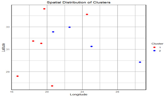
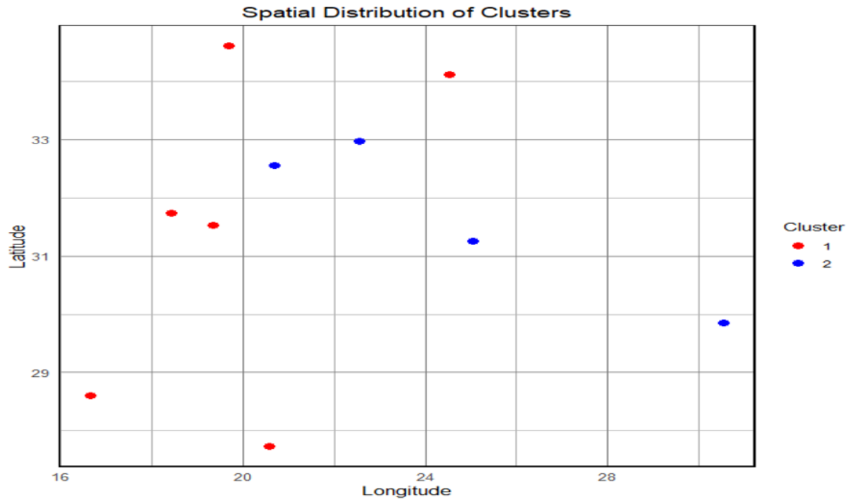
The scatterplot Figure 2 illustrates the spatial distribution of clusters based on station coordinates in terms of latitude and longitude. The two clusters are visually distinct—cluster 1 (shown in red) is primarily located in the western region with lower longitude values. In contrast, cluster 2 (shown in blue) is positioned toward the eastern part of the study area. Lastly, the coverage of the spread of cluster 1 stations reveals a rather wide latitude range, demonstrating greater dispersion, unlike the cluster 2 stations, which are few and geographically concentrated. This spatial differentiation is reflected in the clusters obtained, underscoring the importance of the geographical factor in their formation and highlighting climatic differences among the WASA stations.
Figure 2.
Spatial distribution of station clusters.
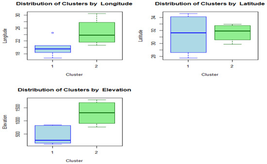
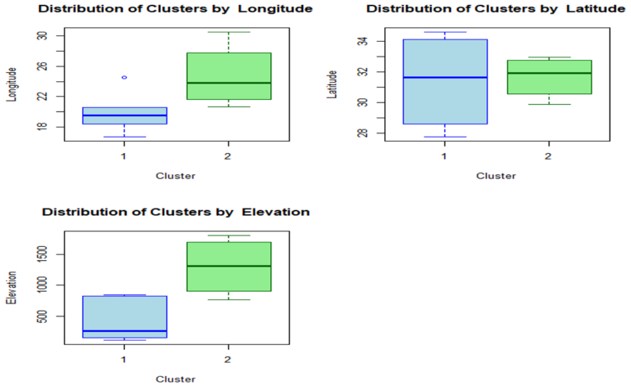
Figure 3 displays the spatial and topographical characteristics of two clusters based on their longitude, latitude, and elevation status. The longitude plot shows that stations in cluster 1 are primarily in a lower-latitude zone, whereas those in cluster 2 are located farther east, with higher longitudes. The plot showing the distribution based on latitude shows that while cluster 1 covers a broader zone, extending further into the northern latitudes, cluster 2 stations are concentrated within a narrower zone of lower latitudes. Finally, based on elevation, a notable difference between the two clusters is observed in Figure 3. In this regard, stations within cluster 1 are concentrated in lower-elevation zones, whereas those within cluster 2 are concentrated in higher-elevation zones. Overall, Figure 3 shows notable differences between clusters, thus supporting a spatial coherence between clusters based on longitude, latitude, and elevation status.
Figure 3.
Distribution of clusters by coordinates and elevation.
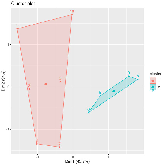
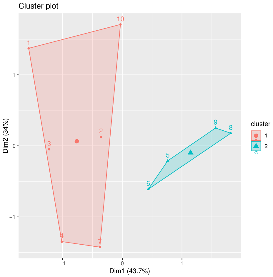
Figure 4 includes two clusters, 1 and 2, with each cluster included in a polygon that denotes the cluster boundary. Here, Dim1 accounts for 43.7% of the variance, while Dim2 accounts for 34%. These values add up to over 77%. Thus, it is evident that this plot includes most of the clusters. In Figure 4, it is evident that the spatial distribution of the clusters is demonstrated through hierarchical methods. All the clusters generated by the dendrogram are clearly separated, demonstrating that hierarchical clustering effectively distinguishes between them. In this plot, it is evident that the clusters are well separated in Dim1, indicating that it is an important dimension for distinguishing between them.
Figure 4.
Hierarchical cluster plot.
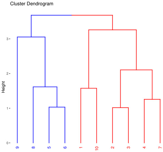
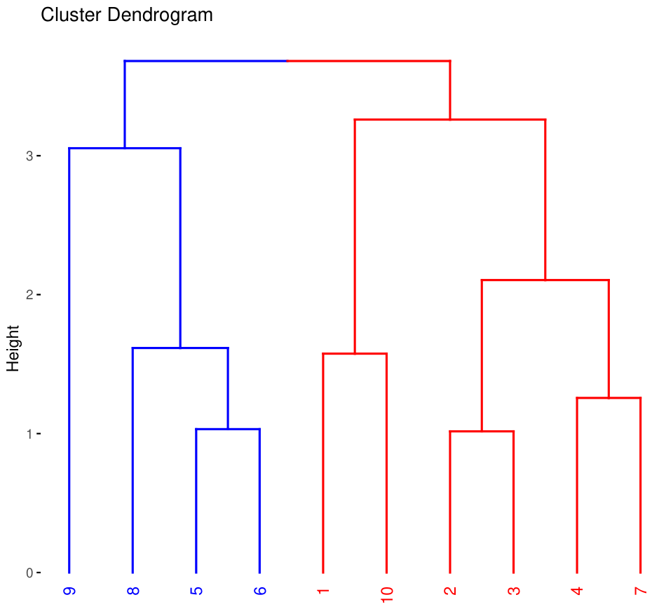
Figure 5 shows a dendrogram for clustering ten different stations labelled from 1 to 10. The vertical axis is labelled “Height,” indicating the degree of dissimilarity or the distance at which clustering occurs. The degree of dissimilarity is higher for points clustered at higher positions than for those clustered at lower positions. From the given dendrogram, two clusters are marked within dashed boxes. The first cluster consists of stations 9, 8, 5, and 6, whereas the second cluster consists of stations 1, 10, 2, 3, 4, and 7.
Figure 5.
The dendrogram.
- Multivariate exploratory data analysis
Table 3 lists the summary statistics of wind data across stations. Many stations exhibit moderate to high variability, with median wind speeds typically 6–7.5 m/s. The highest wind activity comes from stations 3 and 4, while Station 9 is the calmest. The maximum wind speed is close to 24 m/s, suggesting occasional high-wind events.
Table 3.
Summary statistics for wind speed data (stn1 to stn10).
Also, the average values across the stations are quite different as indicated in Table 3. Alternatively, for Station 1 (stn1), the mean is higher than the median, suggesting the data may be right-skewed. Also, the difference between Q3 and the maximum is very high, suggesting the presence of outliers or a long tail.
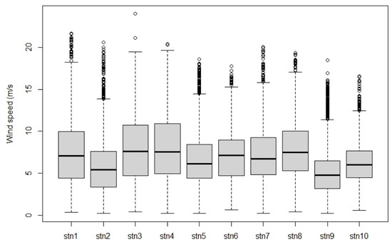
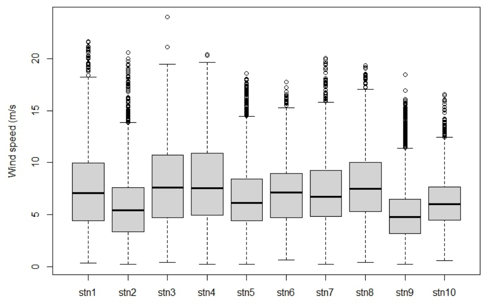
Figure 6 is a boxplot showing the distribution of wind speed (in m/s) across 10 stations (stn1 to stn10). Each box shows the central 50% of the data (interquartile range), the line within the box shows the median wind speed, and the dots represent outliers. Stations such as stn4, stn6, and stn7 exhibit higher wind speeds and greater variability, while others, such as stn1, stn2, and stn8, have lower, more consistent wind speeds.
Figure 6.
Boxplot of the distribution of wind speed (in m/s) across all stations.
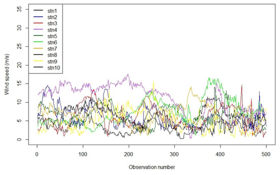
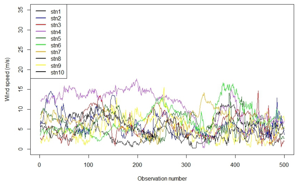
The plot in Figure 7 is a time-series line plot showing the wind speed (in m/s) recorded at 10 different stations over a series of observations. A sample of 500 was taken to improve visualisation of wind speed. Each line represents the variation in wind speed at a specific station, showing temporal fluctuations and variability. The overlapping lines illustrate how wind speed trends differ and coincide between stations during the observed period.
Figure 7.
Time-series plot for all the stations.
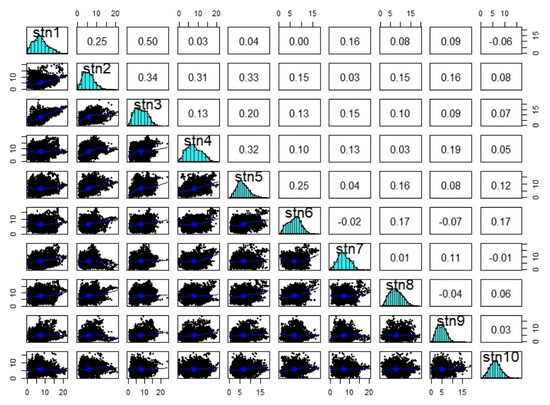
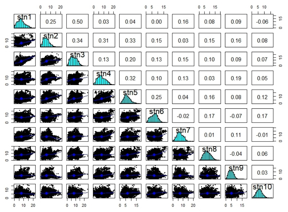
Figure 8 shows a scatterplot matrix combined with histograms and correlation coefficients for wind speed data. This plot is useful for understanding the pairwise relationships and dependencies among wind speed measurements across different stations. The histograms show the wind speed distribution for each station. The scatterplots show pairwise relationships between wind speeds at different stations. Each plot has a fitted smooth curve (blue line) to show trends. Correlation coefficients between wind speeds at pairs of stations are also presented. These values quantify the strength and direction of linear relationships (positive, negative, or near zero). The correlation coefficients are mostly positive but low to moderate (generally below 0.4), indicating a weak linear association. Stations such as stn1 and stn2, or stn2 and stn3, have somewhat higher correlations.
Figure 8.
Correlation plot for all the stations.
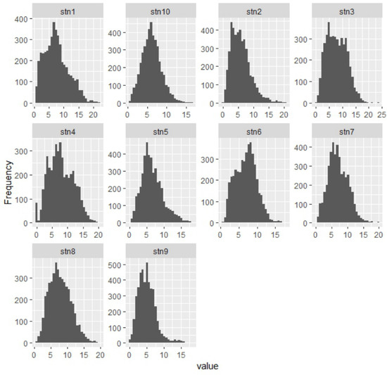
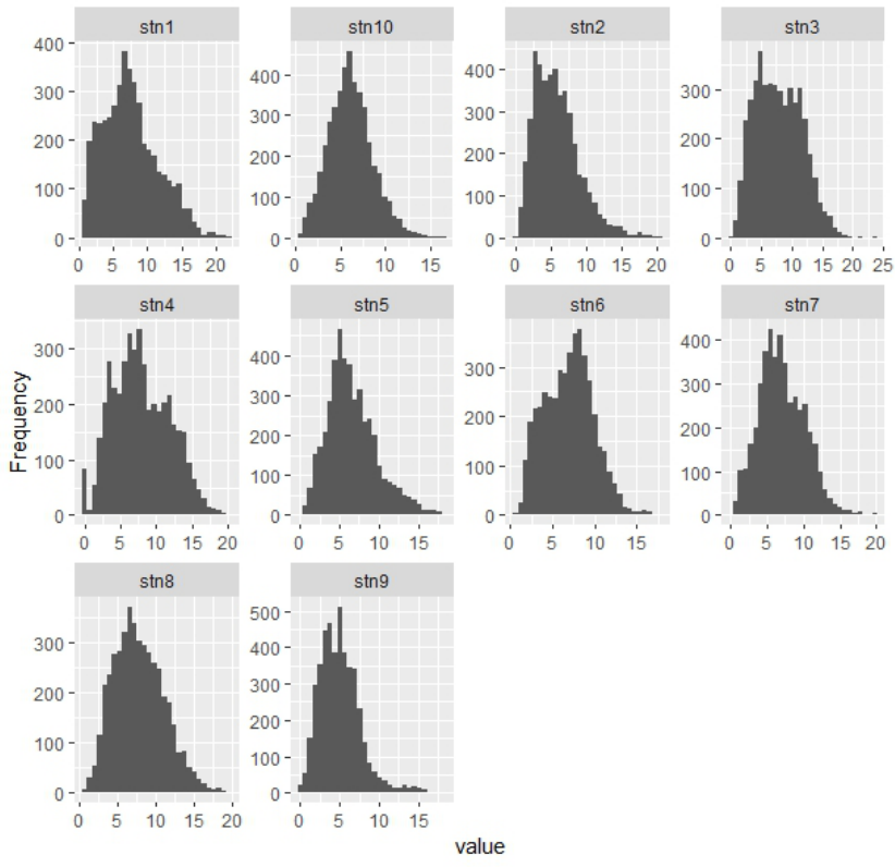
Figure 9 gives a clear visualisation of how wind speed is distributed at each station. Most stations experience wind speeds typically between 0 and 15 m/s, with varying frequencies. Differences in histogram shape suggest variations in local wind speed patterns across stations.
Figure 9.
Histogram of all the stations.
4.2. Results for the Models
The results for the models are presented in the following sections in two stages. Firstly, Section 3.1 presents the results for the linear and Gaussian process (GP) models applied to all possible combinations of training and testing stations, providing a comprehensive evaluation of predictive performance and metrics such as RMSE, NLPD, CVG, and acceptance rate . These results establish the baseline behaviour of the GP models across clusters and highlight the effects of station selection and spatial coverage.
In contrast, Section 3.2 evaluates the hybrid linear–Gaussian process framework. Here, a linear regression model is first estimated to capture large-scale spatio-temporal trends, and a GP is subsequently applied to the residuals to model local deviations. Within this second stage, a variety of covariance structures are rigorously assessed, including Matérn functions with smoothness parameters , as well as exponential and Gaussian covariances. The final covariance choice is determined based on validation performance. Because the hybrid model explicitly separates linear and residual components, the train–test splits, validation folds, and reported metrics differ from Section 3.1. Metrics such as are not always relevant for residual modelling, and certain summary metrics (e.g., CRPS) are computed only where meaningful for the hybrid framework. This structure ensures that the evaluation in Section 3.2 reflects the performance of the hybrid approach in capturing both large-scale trends and local residuals rather than replicating the exhaustive GP-only analysis.
4.2.1. Results for the Linear and GP Models
- Variable selection
Relaxed Lasso is a variation of the Lasso (Least Absolute Shrinkage and Selection Operator) regression method, designed to improve variable selection by reducing the bias introduced by Lasso’s strong penalty. In the first step, Lasso is applied to select a subset of relevant variables by shrinking some coefficients exactly to zero. Then, in the second step, a less-penalised or unpenalised regression (like OLS) is fit only on the selected variables, allowing the model to estimate their coefficients more accurately. This two-stage process helps maintain Lasso’s variable selection strength while improving the accuracy and interpretability of the prediction by relaxing the amount of shrinkage applied.
- Forecast evaluation
We perform modelling using the spTimer package in R, and we use an MCMC approach to estimate the posterior distributions of the model parameters. The following MCMC settings were used: number of iterations (N): 2000; burn-in period: 300 iterations; thinning interval: 1; number of chains: 3; and reporting interval (report): 3. Such settings mean that the program was run for 2000 iterations, of which the initial 300 were considered as burn-in to minimise the impact of initial values. Thinning of 1 means that the entire set of post-burn samples is utilised for posterior analysis. Running the chains enables convergence diagnosis, ensuring proper parameter evaluation. The report = 3 settings ensure that the algorithm reports every third iteration, thus enabling tracking of the execution of the sampling function. Such settings ensure an appropriate trade-off between computational efficiency and the sample size required to approximate the posterior distribution.
Evaluation for cluster 1
- Training and testing for cluster 1
In cluster 1, we use the ratio to generate all possible combinations of data for the test set, with test set sizes ranging from one to three samples. We used the configurations , and , which resulted in 41 unique train–test partitions. In each configuration, the selected subset of stations served as the test set and the remaining stations were used for training. The objective of this exhaustive enumeration is to evaluate the robustness of spatial generalisation with respect to the specific choice of held-out stations. By considering every possible hold-out combination, we eliminate randomness due to fold assignment and provide a complete assessment of how sensitive model performance is to station selection. The combinations resulting from the testing and training sets are in Table A1 in the Appendix.
- Results for cluster 1
Table 4 summarises predictive performance across all 41 spatial hold-out configurations. When a single station is held out (leave-one-station-out validation), the model is trained on five stations and evaluated on one. As expected, this setting yields the lowest RMSE, MAE, NLPD, and CRPS values because the training set is largest and the extrapolation domain is minimal. When two stations are held out, predictive performance degrades moderately across all proper scoring rules. This reflects both the reduced amount of spatial information available for training and the increased geographic extent of the test domain. The most challenging setting occurs when three stations are held out. In this case, the model is trained on only half of the available stations and must extrapolate to a substantially larger unseen spatial region. Consequently, RMSE, MAE, CRPS, and NLPD increase consistently in relation to cases of one and two stations.
Table 4.
Performance metrics for different station combinations (compact view).
This monotonic degradation pattern indicates that performance is sensitive to the degree of spatial data removal rather than to any specific station combination. Importantly, coverage (CVG) remains stable across configurations, suggesting that predictive uncertainty is well-calibrated even as extrapolation difficulty increases. The variability observed within each group (for example, across different three-station subsets) reflects heterogeneity in spatial information content across stations, highlighting that some station combinations are inherently more informative for spatial interpolation than others. Therefore, Table 4 quantifies how predictive accuracy deteriorates as the spatial extrapolation task becomes more challenging. In this sense, the table illustrates the sensitivity of model performance to the degree of spatial data removal, providing a structured robustness assessment of spatial extrapolation performance. The metric quantifies the relative contribution of each train–test combination within the fusion scheme. Specifically, for combination j, is defined as
where represents the weight or influence assigned to combination j based on its predictive performance. CVG and other metrics are used to determine in a manner that emphasizes well-performing combinations. The resulting values are expressed as percentages, highlighting which combinations contribute the most to the overall fused prediction. It represents the acceptance rate in the GPR fusion scheme, highlighting the train–test combinations that contribute most reliably to the final predictive ensemble. The metric further highlights the combinations that contribute the most within the fusion scheme, with certain station sets, such as 2, 3, 3–5, 3–6, and 2–5–6, receiving higher relevance scores, suggesting that these combinations provide more informative predictors for the model.
- Prediction plots
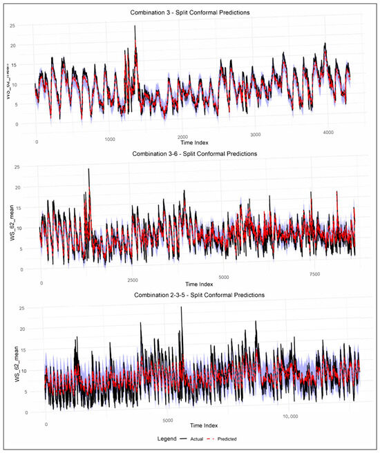
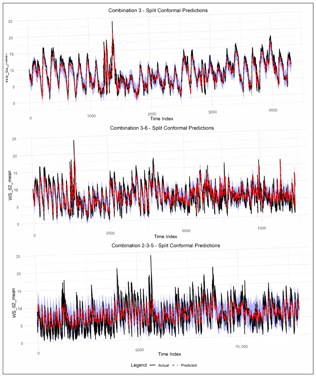
Pairwise combinations tend to report higher NLPD, wider prediction intervals, and greater RMSEs as model complexity increases due to greater spatial variability. This phenomenon is reinforced when visualised within Figure 10, where combined stations report wider bands of conformal prediction and less smooth trends for the mean trajectories, while the prediction intervals report perfectly well-calibrated performance across the different combinations, reporting the desired true coverage of 95% as affirmed by the CVG values reported within Table 4.
Figure 10.
Prediction plots for cluster 1 high-performing stations.
Importantly, the adaptive extension of the prediction interval in the regime of high wind variability, evident from Figure 10, shows the capability of the split conformal method in handling the dynamic uncertainty without sacrificing the guarantees. These examples reveal an interesting balance between the sharpness of predictions and the level of aggregation, indicating that although aggregation can be valuable, it might also entail a penalty in the loss of local wind dynamics, which is of principal importance.
Evaluation for cluster 2
- Testing and Training sets
The training set is the data used to train the model, allowing it to learn patterns and relationships. In contrast, the testing set is a separate portion of data used to assess how well the model performs on new, unseen inputs. By splitting data into these two sets, we can ensure the model learns effectively without simply memorising the data, helping to avoid overfitting and giving a more accurate measure of how the model will perform in real-world scenarios. Table A2 in the Appendix shows the test–train sets for cluster 2.
To evaluate the model’s performance and generalisation, two data-splitting strategies were employed, each using combinations of four spatial locations. We used the two configurations , which denote combinations in which subsets of four components are split into training and testing sets. These combinations provide a systematic way to assess the model’s robustness under varying data availability scenarios and to evaluate predictive performance across different spatial partitions.
- Results for Cluster 2
Table A3 presents a comparative evaluation of the performance of the model in various training and testing configurations using key statistical metrics: Root Mean Square Error (RMSE), Mean Absolute Error (MAE), continuous ranked probability score (CRPS), probability of prediction interval coverage (PICP), negative log predictive density (NLPD), normalised average width of prediction interval (PINAW), and normalised average deviation of prediction interval (PINAD).
From Table 5, among all configurations, Combination 1 achieves the best overall performance, yielding the lowest values of NLPD, RMSE, MAE, and CRPS, together with the narrowest prediction intervals (PINAW). Combination 2 shows comparable but slightly inferior performance, while Combination 3 and Combination 4 exhibit noticeably higher error metrics and wider prediction intervals. Pairwise station combinations generally lead to higher prediction errors and greater uncertainty than single-station cases, with Combination 2–3 showing the weakest performance across most metrics.
Table 5.
Performance metrics for different combinations (best in bold).
Across all configurations, the empirical coverage (CVG) remains close to the nominal level of 0.95, indicating that the probabilistic forecasts are well-calibrated regardless of the station combination. The relative improvement metric indicates consistent performance gains over the linear baseline, with the largest improvements observed for single-station configurations.
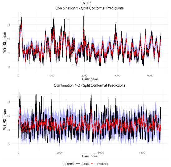
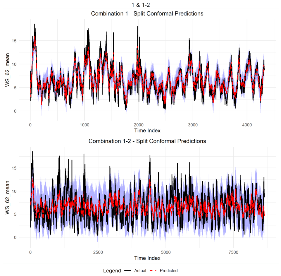
Figure 11 presents the split conformal prediction results for Combination 1 and Combination 1–2, while the corresponding quantitative performance metrics are reported in Table 5. For Combination 1, the predicted mean closely tracks the observed wind speed, with relatively narrow prediction intervals, consistent with the low RMSE (1.15), MAE (0.88), CRPS (0.76), and PINAW (0.25) values reported in the table. In contrast, Combination 1–2 exhibits wider prediction intervals and increased variability in the predicted mean, which aligns with the higher RMSE (2.44), MAE (1.97), CRPS (1.39), and PINAW (0.51) observed in Table 5. In both cases, the empirical coverage shown in Figure 11 is consistent with the nominal level, in agreement with the CVG value of approximately 0.95 reported in the table. The split conformal prediction method provides prediction intervals (shown as shaded regions) that effectively capture the variability in the observed wind speed data (black line). The predicted values (red dashed line) closely follow the actual measurements, and the uncertainty bands adapt over time, widening during more volatile periods and narrowing during more stable periods. This shows that split conformal prediction generates well-calibrated, dynamic-width intervals that reflect the true uncertainty in predictions across disparate time indices.
Figure 11.
Prediction plots for cluster 2 high-performing stations.
4.2.2. Results for the Hybrid Linear–Gaussian Process
- Cluster setup
The dataset used for the hybrid model was divided into two clusters based on elevation, longitude, and latitude to account for spatial heterogeneity in wind behaviour. Cluster 1 consists of lower to mid-elevation stations (152–848 m), while cluster 2 contains higher-elevation stations (770–1806 m). This is important for accounting for heterogeneity in wind speed dynamics. Model performance was evaluated separately for each cluster using multiple validation splits. This strategy allows for assessment of whether the proposed hybrid framework performs consistently across regimes with different statistical and physical characteristics.
- Validation Setup
The proposed hybrid modelling framework was evaluated using a two-fold validation strategy. A leave-one-station-out cross-validation approach was used to evaluate model performance. In each iteration, data from one wind station were withheld for validation, while the remaining stations were used for model training. This procedure was repeated until each station had served as the validation site once. For cluster 1 (total sample size 25,914), each validation set comprised 16.7% of the available observations (4319 samples per split), and for cluster 2 (total sample size 17,276), each validation set comprised 25% of the available observations (4319 samples per split). For each split, a two-stage process was used. First, a linear regression model was estimated to account for large-scale spatio-temporal effects, followed by a GP analysis of the residuals. A variety of covariance structures were rigorously evaluated within the second stage, including several Matérn covariance functions with smoothness and ; an exponential covariance; and a Gaussian covariance. The best-performing covariance structure is based on validation performance.
Results for Cluster 1: Weak or Unstable Residual Structure
- Predictive Performance
In respect of cluster 1, the improved linear–Gaussian process (GP) hybrid model performance was reported as mixed, with varying levels of improvement depending on the residual errors it could model relative to the purely linear model. From the results presented in Table 6, the three distinct validation set RMSEs were 3.127, 21.779, and 2.828, while the linear model reported values were 3.125, 21.431, and 2.844. Here, the enhancements reported ranged from −1.622 to 0.576, indicating that this approach is indeed useful for modelling the nonlinear residuals. However, the overall improvement is limited by the varying spatial residuals in cluster 1. In one of the folds, it reports an improvement of 0.576, despite the overall spatial correlation in the residuals.
Table 6.
Model performance metrics by clusters and validations.
- Covariance Selection and Residual Structure
In all three model validation cases, the Gaussian (squared exponential) covariance was selected as optimal. This suggests that the residuals of cluster 1 could be best modelled as having a stationary covariance structure. Additionally, the negative improvement in the GP fold indicates that the residuals’ spatial structure is neither strong nor stationary, resulting in little improvement from the GP method. Covariance-based feature selection cannot always adequately compensate for residual heterogeneity.
- Probabilistic Forecast Quality
The hybrid method provided well-calibrated uncertainty estimates. The coverage (CVG) was kept at 0.95 for all the folds, and the PINAW values ranged from 0.465 to 2.511. Low PINAD values across most folds indicate little bias in interval centring. This shows that even when point prediction was not significantly improved, the GP component still provided good predictions; hence, decisions could be made accordingly.
- Implications for Wind Speed Forecasting
The results for cluster 1 should be kept in mind for the practical application of the wind forecast method. In particular, the usefulness of the hybrid GP modelling method depends on the spatial coherence of the residuals; a lack of heterogeneity in the residuals could prevent efficient RMSE improvement within the clusters. The selection of covariance should be based on validation performance, but this may require non-stationary and/or multi-scale kernels for more accurate terrain-effect modelling. Probabilistic forecasts remain robust, and a small improvement in point predictions underscores the scope for risk-informed decision-making with hybrid models, especially in wind energy applications. The findings from cluster 1 highlight that modelling strategies should vary across clusters, accounting for trends and residual spatial structures, especially in complex terrain and heterogeneous winds.
Results for Cluster 2: Strong Spatio-Temporal Dependence
- Predictive performance
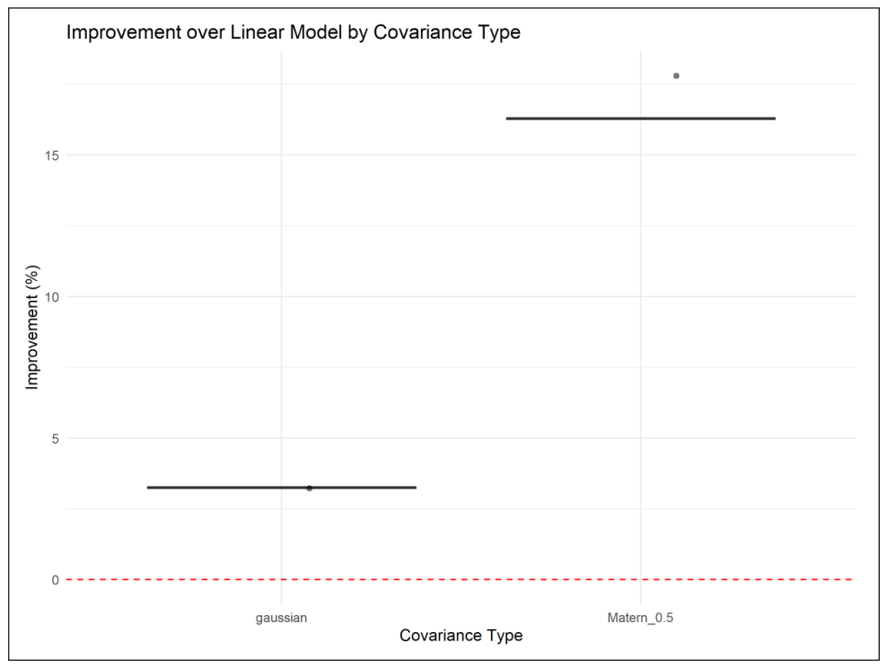
In both sets of validation data, the proposed hybrid linear–GP model significantly performed better than the linear-only model, validating the presence of underlying spatio-temporal correlation in the residual wind speed field (Table 6). For the first validation set, the proposed model showed improved performance, achieving an RMSE of 2.51, compared with the linear model, which achieved an RMSE of 2.99. The performance improvements in the proposed model were hence 16.3%. On the second set, the improvements were slightly lower, at 3.2%, as indicated by the reduced RMSE from 2.39 to 2.31.
- Covariance Selection and Residual Structure
Different optimal covariance structures were selected based on the validation splits reported by the machine learning algorithm, using the automatic covariance structure selection method implemented in the code. In the first validation set, the Matérn covariance structure with was consistently selected, while in the second set, the Gaussian covariance structure was preferred. The Matérn covariance structure essentially corresponds to a rough, even non-differentiable, stochastic process, which is typically preferred for modelling abrupt changes in the underlying dynamics, for instance, those characterising localised variability in the wind field. The optimal structure found for the first set suggests that the dynamics of the residual wind field were characterised by particularly rough variability, potentially linked to factors such as gustiness and rapid regime changes. On the contrary, the optimal choice of the Gaussian kernel was observed in the second set, where the proportion of the original variability explained by the linear model was also particularly large.
- Probabilistic Forecast Quality
Aside from point prediction accuracy, the hybrid models also demonstrated excellent probabilistic performance. Also, the Matérn performed best in terms of the smallest negative log predictive density, well-centred prediction intervals, and almost nominal empirical coverage of about 95%. Even though the prediction intervals generated by the Gaussian kernel were narrower and the CRPS was slightly reduced, the model also showed some underdispersion, indicating overconfidence in the predictions. These findings reveal a balance between point prediction accuracy and probabilistic calibration, with rougher covariance structures yielding a more realistic quantification of uncertainty in wind speed predictions.
- Implications for Wind Speed Forecasting
The results show the capability of hybrid linear-GP approaches with adaptive covariance selection in spatio-temporal prediction of wind speed while being physically consistent. The linear model demonstrates its capability to capture larger trends, while the GP model captures the localised stochastic component. The tendency toward rough covariance structures supports the non-smooth nature of the underlying wind speed processes, justifying the use of Matérn kernels in this context. The presented model offers greater prediction accuracy, more precise quantification of uncertainty, and greater interpretability of predictions than traditional linear models.
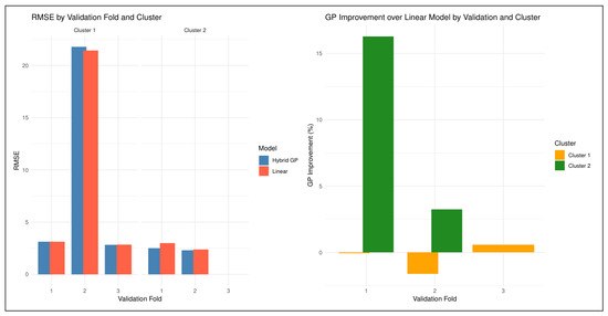
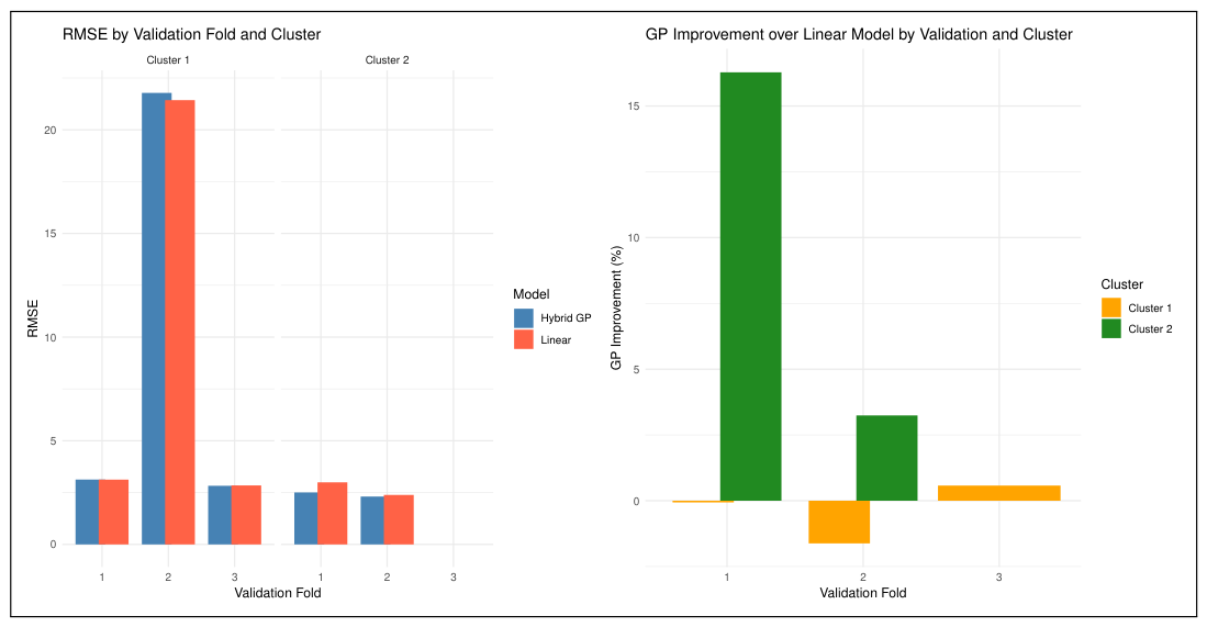
As shown in Figure 12, the figure compares the predictive performance of the linear and hybrid GP regression models across two data clusters and various validation sets. The left-hand side of the figure illustrates a representation of the Root Mean Square Error (RMSE) for the linear model and the hybrid GP model. In cluster 1, the RMSE improvements are inconsistent: one validation fold shows a small gain, while the others show minor degradation relative to the linear model. In cluster 2, all validation folds show meaningful RMSE reductions with the GP component, emphasizing the strong spatio-temporal correlations in high-elevation stations. As is apparent, the RMSE is a vital measure that effectively quantifies error. As such, lower error values are desirable compared to higher ones. This figure effectively compares the relative performance of including the GP model in improving overall wind speed prediction across different data clusters. On the other hand, the right-hand side of Figure 12 demonstrates the percentage improvement in the hybrid GP model over the basic linear model.
Figure 12.
Comparison of predictive performance between linear and hybrid GP models across clusters and validation sets.
5. Discussion
5.1. Discussion of Results
The suggested hybrid approach was evaluated on two different clusters based on wind speed data. The hybrid linear–Gaussian process approach showed different levels of performance across the two clusters distinguished by clustering.
Cluster 1 (low elevation/weak residuals): In the three validation groups from cluster 1, GP residual modelling yielded contrasting results. For validation 1 and 2, the use of the Gaussian process slightly undermined forecast accuracy, with RMSE changes of −0.065% and −1.622%, respectively. This finding agrees with the presence of high levels of noise in the residual terms in validation 2, as evidenced by the high NLPD value of 185.534. Only for validation 3, the GP showed slight gains (+0.576%) due to lower RMSE and MAE values. This suggests that, in a loosely structured wind regime, there is little to learn from residuals, and adding a Gaussian process will not necessarily improve the results. Predictive performance was still satisfactory overall, with well-calibrated probabilistic predictions, as indicated by a stable calibration of 0.95.
Cluster 2 (high altitude/residuals are strong): On the other hand, for cluster 2, the hybrid model always performed well. In the two validation rounds, the GP model reduced the RMSE by 16.279% and 3.242% compared to the linear model. Small PINAW and PINAD values were observed, indicating that the hybrid model’s predictive intervals were well-calibrated. It is important to note that the covariance function mattered because it determined the model’s predictive power. Specifically, the use of the kernel outperformed in validation 1, while validation 2 only needed a Gaussian kernel. The probabilistic criteria for the CRPS and NLPD indicated that the hybrid model provided accurate uncertainty estimates.
On the whole, these findings highlight the importance of regime sensitivity when evaluating the predictive power of GP residual modelling. While additional complexity will be meaningless for regions with low spatial correlation (cluster 1), it becomes highly valuable for regimes with high variability (cluster 2). In practical terms, these findings underscore the importance of regime-aware modelling methodologies. Overusing sophisticated stochastic models can lead to unnecessary computational costs and reduced forecasting accuracy.
5.2. Limitations and Future Work
Firstly, the assumption of stationarity within the clusters generated by the Gaussian process residual model does not account for regime shifts, which may be inherent to atmospheric processes. This problem might be especially relevant for cluster 1, based on the validation outcomes. The second potential drawback of the Gaussian process approach is its sensitivity to sparsity/outliers, which can be observed occasionally during model validation. It must be acknowledged that the problem can be alleviated by implementing adaptive covariance estimation. Finally, although the two-stage technique offers greater interpretability and computational efficiency, no physical constraints were incorporated into the model.
6. Conclusions
This study used a hybrid linear–Gaussian process model for short-term prediction of wind speed data. The proposed model was tested for clustering wind speed datasets based on elevation and geographic coordinates. The main results obtained show that the applicability of the hybrid model strongly relies on the properties of the cluster. In particular, residual modelling via Gaussian processes did not yield substantial benefits in cluster 1; on the contrary, in several validation exercises, it caused even minor performance losses due to the low-residual structure of the cluster.
On the other hand, in cluster 2, consistent advantages of using Gaussian processes were observed across both point and probabilistic predictions, with up to a 16.3% improvement in RMSE. Another important finding was the role of kernel selection and the need to adapt this process to each cluster, as evidenced by the superior performance of the adaptive Gaussian process over the adaptive Matérn kernel with . As for probabilistic prediction, good calibration was observed across all experiments (coverage probability of 0.95). This demonstrates that the hybrid model provides reliable uncertainty estimates suitable for operational decision-making.
Operationally speaking, the findings suggest that regime-specific modelling is valid. In other words, there is no need to employ Gaussian process residuals indiscriminately in regions with consistent wind regimes, where this might not only prove superfluous but even detrimental. At the same time, there is immense potential to utilise them in regions with prominent spatial variation. Overall, the hybrid approach is a balanced solution that maintains transparency, considers spatial dependence, and ensures accurate uncertainty estimation.
Author Contributions
Conceptualisation, T.H.T. and C.S.; methodology, T.H.T.; software, T.H.T.; validation, T.H.T., C.S., T.B.D. and S.N.; formal analysis, T.H.T.; investigation, T.H.T., C.S., T.B.D. and S.N.; data curation, T.H.T.; writing—original draft preparation, T.H.T.; writing—review and editing, T.H.T., C.S., T.B.D. and S.N.; visualisation, T.H.T.; supervision, C.S., T.B.D. and S.N.; project administration, C.S., T.B.D. and S.N. All authors have read and agreed to the published version of the manuscript.
Funding
This research received no external funding.
Data Availability Statement
The data in brief can be accessed at https://github.com/csigauke/A-Hybrid-Linear--Gaussian-Process-Framework-for-Spatio-Temporal-Wind-Speed-Forecasting (accessed on 16 January 2025).
Acknowledgments
The authors thank the anonymous reviewers for their helpful comments on this paper.
Conflicts of Interest
The authors declare no conflicts of interest.
Abbreviations
The following abbreviations are used in this manuscript:
| MAE | Mean Absolute Error |
| MASE | Mean Absolute Scaled Error |
| RMSE | Root Mean Squared Error |
| MCMC | Markov Chain Monte Carlo |
| CRPS | Continuous Ranked Probability Score |
| PICP | Probability of Prediction Interval Coverage |
| NLPD | Negative Log Predictive Density |
| PINAW | Normalised Average Width of Prediction Interval |
| PINAD | Normalised Average Deviation of Prediction Interval |
Appendix A. Supplementary Results
Table A1.
Testing and training set combinations (grouped into 6C1–6C2 and 6C3).
Table A2.
Testing and training set combinations for cluster 2.
Table A3.
Model performance for LM and GPR across station combinations.
- Hybrid model plots
Figure A1.
RMSE for cluster 1.
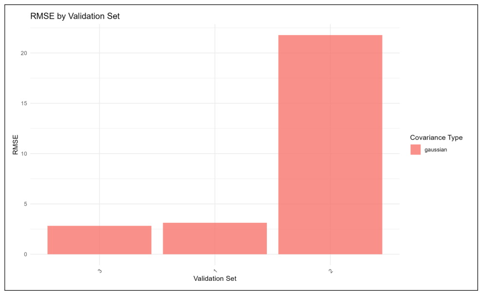
Figure A2.
RMSE for cluster 2.
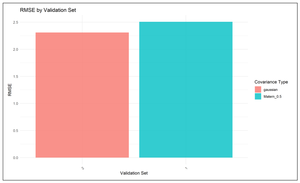
Figure A3.
Improvement for cluster 1.
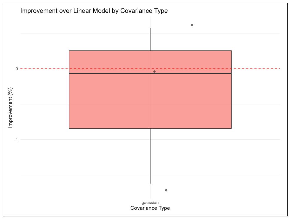
Figure A4.
Improvement for cluster 2.
Appendix B. Modelling Specification: An Extensive Hierarchical Bayesian Formulation with MCMC Sampling
Appendix B.1. Hybrid Model Specification
Let denote the response variable wind speed at location and time . The complete model is
where
- is a vector of covariates;
- are regression coefficients;
- is a zero-mean Gaussian process;
- is the measurement error (nugget effect);
- is the covariance function with parameters .
Appendix B.2. Two-Stage Estimation Procedure
Appendix B.2.1. Stage 1: Linear Regression
The very first attempt at modelling a spatio-temporal response variable is to consider the linear regression models. First, estimate the linear component via ordinary least squares:
The linear predictions are
Residuals for GP modelling:
Appendix B.2.2. Stage 2: Gaussian Process on Residuals
Model the residuals as follows:
where .
Appendix B.3. Covariance Structures
Appendix B.3.1. General Form of Covariance Functions
For spatio-temporal modelling, we consider separable covariance functions:
where is the marginal variance.
Appendix B.3.2. Matérn Family of Covariance Functions
The Matérn covariance function is defined as
where
- is the Euclidean distance;
- is the smoothness parameter;
- is the range parameter;
- is the variance parameter;
- is the modified Bessel function of the second kind.
Appendix B.3.3. Special Cases
- 1.
- Exponential covariance ():
- 2.
- Matérn with :
- 3.
- Matérn with :
- 4.
- Gaussian/squared exponential ():
- Exponential covariance () models rough processes with less smoothness.
- Gaussian covariance () assumes very smooth processes.
- Matérn covariance with intermediate balances smoothness and flexibility.
Appendix B.3.4. Rational Quadratic Covariance
Appendix B.4. Likelihood and Estimation
Appendix B.4.1. Gaussian Process Likelihood
For n observations , the log-likelihood is
where is the covariance matrix with entries .
Appendix B.4.2. Maximum Likelihood Estimation
The MLE estimates are obtained by
Appendix B.4.3. Predictive Distribution
For a new location , the predictive distribution is Gaussian:
with
where .
Appendix B.5. Hierarchical Bayesian Formulation
Appendix B.5.1. Complete Bayesian Model
Appendix B.5.2. Posterior Distribution
Appendix B.5.3. Gibbs Sampling
- 1.
- Sample (conjugate):
- 2.
- Sample (conjugate):
- 3.
- Sample covariance parameters (Metropolis–Hastings):Accept with probability:
Appendix B.6. Model Comparison and Selection
Appendix B.6.1. Information Criteria
Appendix B.6.2. Cross-Validation
For K-fold CV:
Appendix B.7. Uncertainty Quantification
- Prediction Intervals
For a new location , the predictive distribution of the response is Gaussian. The prediction interval:
where . This provides both a point prediction () and an uncertainty measure () for the new location.
Appendix B.8. Conformal Prediction
- 1.
- Compute residuals: .
- 2.
- Find -quantile: .
- 3.
- Prediction interval: .
Appendix B.9. Computational Aspects
Appendix B.9.1. Scalability Challenges
Exact GP: . Solutions:
- Low-rank approximations: , .
- Sparse covariance methods.
- Stochastic Variational Inference.
Appendix B.9.2. Numerical Stability
- Add jitter: .
- Use Cholesky decomposition with pivoting.
- Compute log-determinant via Cholesky factors.
Appendix B.10. Theoretical Properties
Appendix B.10.1. Consistency
Under regularity conditions, as :
Appendix B.10.2. Asymptotic Normality
For fixed-domain asymptotics:
where is the Fisher information matrix.
References
- Yang, M.; Jiang, Y.; Che, J.; Han, Z.; Lv, Q. Short-Term Forecasting of Wind Power Based on Error Traceability and Numerical Weather Prediction Wind Speed Correction. Electronics 2024, 13, 1559. [Google Scholar] [CrossRef] [Scilit]
- Szostek, K.; Mazur, D.; Drałus, G.; Kusznier, J. Analysis of the Effectiveness of ARIMA, SARIMA, and SVR Models in Time Series Forecasting: A Case Study of Wind Farm Energy Production. Energies 2024, 17, 4803. [Google Scholar] [CrossRef] [Scilit]
- Xu, J.; Xiao, Z.; Lin, Z.; Li, M. System bias correction of short-term hub-height wind forecasts using the Kalman filter. Prot. Control Mod. Power Syst. 2021, 6, 37. [Google Scholar] [CrossRef] [Scilit]
- Liu, Z.; Guo, H.; Zhang, Y.; Zuo, Z. A Comprehensive Review of Wind Power Prediction Based on Machine Learning: Models, Applications, and Challenges. Energies 2025, 18, 350. [Google Scholar] [CrossRef] [Scilit]
- Che, G.; Zhou, D.; Wang, R.; Zhou, L.; Zhang, H.; Yu, S. Wind Energy Assessment in Forested Regions Based on the Combination of WRF and LSTM-Attention Models. Sustainability 2024, 16, 898. [Google Scholar] [CrossRef] [Scilit]
- Bessa, R.J.; Miranda, V.; Gama, J. The Role of Predictive Distributions in Modern Wind Power Forecasting Frameworks. Int. J. Forecast. 2022, 38, 601–615. [Google Scholar] [CrossRef] [Scilit]
- Elshaboury, N.; Elmousalami, H. Wind speed and power forecasting using Bayesian optimised machine learning models in Gabal Al-Zayt, Egypt. Sci. Rep. 2025, 15, 28500. [Google Scholar] [CrossRef] [Scilit] [PubMed]
- Yang, Q.; Huang, G.; Li, T.; Xu, Y.; Pan, J. A Novel Short-Term Wind Speed Prediction Method Based on Hybrid Statistical-Artificial Intelligence Model with Empirical Wavelet Transform and Hyperparameter Optimization. J. Wind Eng. Ind. Aerodyn. 2023, 239, 105499. [Google Scholar] [CrossRef] [Scilit]
- Cai, H.; Jia, X.; Feng, J.; Li, W.; Hsu, Y.-M.; Lee, J. Gaussian Process Regression for Numerical Wind Speed Prediction Enhancement. Renew. Energy 2020, 146, 2112–2123. [Google Scholar] [CrossRef] [Scilit]
- Heaton, M.J.; Gelfand, A.E.; Vecchia, D.J.; Guinness, J.R. A Case Study Competition Among Methods for Analysing Large Spatial Data. J. Agric. Biol. Environ. Stat. 2019, 24, 398–425. [Google Scholar] [CrossRef] [Scilit] [PubMed]
- Wang, B.; Yan, L.; Rong, Q.; Chen, J.; Shen, P.; Duan, X. Dynamic Gaussian Process Regression for Spatio-Temporal Data Based on Local Clustering. Chin. J. Aeronaut. 2024, 37, 245–257. [Google Scholar] [CrossRef] [Scilit]
- Sigauke, C.; Chandiwana, E.; Bere, A. Spatio-Temporal forecasting of global horizontal Irradiance Using Bayesian Inference. Appl. Sci. 2023, 13, 201. [Google Scholar] [CrossRef] [Scilit]
- Hu, S.; Xiang, Y.; Zhang, H.; Xie, S.; Li, J.; Gu, C.; Sun, W.; Liu, J. Hybrid Forecasting Method for Wind Power Integrating Spatial Correlation and Corrected Numerical Weather Prediction. Appl. Energy 2021, 293, 116951. [Google Scholar] [CrossRef] [Scilit]
- Liao, Q.; Cao, D.; Chen, Z.; Blaabjerg, F.; Hu, W. Probabilistic Wind Power Forecasting for Newly-Built Wind Farms Based on Multi-Task Gaussian Process Method. Renew. Energy 2023, 217, 119054. [Google Scholar] [CrossRef] [Scilit]
- CSIR. WASA Data Portal. Available online: https://wasadata.csir.co.za/wasa1/WASAData?pscreen=nwa&pemail=nimo@risoe.dtu.dk (accessed on 16 January 2025).
- Hopkins, B.; Skellam, J.G. A new method for determining the type of distribution of plant individuals. Ann. Bot. 1954, 18, 213–227. [Google Scholar] [CrossRef] [Scilit]
- Meinshausen, N. Relaxed Lasso. Comput. Stat. Data Anal. 2007, 52, 374–393. [Google Scholar] [CrossRef] [Scilit]
- Williams, C.K.I.; Rasmussen, C.E. Gaussian Processes for Machine Learning; MIT Press: Cambridge, MA, USA, 2006; Available online: http://www.gaussianprocess.org/gpml/ (accessed on 23 July 2025).
- Gneiting, T.; Raftery, A.E. Strictly Proper Scoring Rules, Prediction, and Estimation. J. Am. Stat. Assoc. 2007, 102, 359–378. [Google Scholar] [CrossRef] [Scilit]

Disclaimer/Publisher’s Note: The statements, opinions and data contained in all publications are solely those of the individual author(s) and contributor(s) and not of MDPI and/or the editor(s). MDPI and/or the editor(s) disclaim responsibility for any injury to people or property resulting from any ideas, methods, instructions or products referred to in the content. |
© 2026 by the authors. Licensee MDPI, Basel, Switzerland. This article is an open access article distributed under the terms and conditions of the Creative Commons Attribution (CC BY) license.