Garbage In, Garbage Out? The Impact of Data Quality on the Performance of Financial Distress Prediction Models

Highlights

What are the main findings?

• Economically grounded data preparation substantially improves the predictive performance of financial distress models across most classification methods, with average gains of approximately 15.6 percentage points in accuracy and 26.9 percentage points in specificity across all six modelling techniques examined.
• The contribution of data quality to predictive performance amounts to roughly half the performance variation attributable to algorithm choice, supporting the “garbage in, garbage out” principle: models trained on raw, unprocessed financial data consistently underperform their counterparts trained on cleaned and validated data under identical modelling conditions, confirming that input data quality is a major but underexplored driver of model reliability.

What are the implications of the main findings?

• For researchers, preprocessing decisions, including economic plausibility screening, missing value treatment, and class balancing, should be treated as substantive methodological choices and reported transparently, as they materially affect model outcomes and the comparability of findings.
• For practitioners in banking, auditing, and corporate risk management, structured data validation and economically grounded preprocessing should be considered integral components of financial distress model development, as algorithm optimisation alone is insufficient to achieve reliable predictive performance when input data quality is poor.

Abstract

Financial distress prediction remains a central topic in corporate finance and risk management, with extensive research devoted to improving classification accuracy through increasingly sophisticated statistical and machine learning techniques. Nevertheless, the influence of data preparation on predictive performance has received comparatively less systematic attention. This study examines how an economically grounded data-preparation process affects the predictive performance of selected statistical and machine-learning models dedicated to predicting corporate financial distress. Using the chosen financial ratios, generally accepted indicators of corporate financial stability and economic performance, financial distress models are estimated on both raw, unprocessed input data and pre-processed data involving the exclusion of economically implausible accounting values, treatment of missing observations, and class balancing. In light of the above, the study adopts a structured methodological approach to assess the predictive performance of selected classification models, namely decision tree algorithms (CART, CHAID, and C5.0), artificial neural networks (ANNs), logistic regression (LR), and linear discriminant analysis (DA), using confusion-matrix–based evaluation and a comprehensive set of evaluation measures. The results suggest that the process of input data preparation is a critical factor, significantly improving the predictive performance of financial distress prediction models across most modelling techniques employed. The most pronounced gains are observed in decision tree models. ANNs also demonstrate marked improvement after input data preparation, whereas LR benefits more moderately, and linear DA remains limited despite preprocessing. The average gain in accuracy across all six modelling techniques, calculated as the difference between pre-processed and raw performance for each method and averaged across methods, was approximately 15.6 percentage points, with specificity improving by approximately 26.9 percentage points on average, amounting to roughly half the performance variation attributable to algorithm choice, which underscores that data preparation is a primary determinant of model reliability alongside algorithm selection. A step-level detailed analysis further shows that missing value imputation is the dominant driver of improvement for tree-based models, while class balancing contributes most for ANNs and logistic regression. The findings highlight that reliable financial distress prediction depends not only on technique selection but also on the consistency and economic plausibility of the input data, underscoring the central role of structured data preparation in developing robust early-warning models.

1. Introduction

Companies’ financial difficulties constitute a critical indicator of their financial health and may be a significant driver of economic instability, with consequences for company owners, employees, investors, creditors, suppliers, and governmental bodies. In contrast, a financially healthy company possesses sufficient liquidity to meet its obligations and can respond flexibly to potential changes in the economic environment without jeopardising its operations [1], while consistently achieving an adequate return on invested capital given the risks associated with its business activities [2]. Early identification of financial deterioration is therefore crucial, as it enables stakeholders to implement preventive restructuring measures and thereby limit the broader economic consequences of company failure [3,4,5]. For this reason, the development of reliable financial distress prediction models remains a core topic in financial economics and applied corporate risk management [6,7].

Financial distress prediction models are widely used by investors, creditors, auditors, regulators, and corporate managers, and their outputs often inform credit allocation, restructuring decisions, and regulatory supervision. Consequently, the reliability and stability of these models are of substantial practical and economic importance [8] and may become even more critical under crisis conditions and regime shifts, when model effectiveness can deteriorate and early-warning signals may change [9].

Over the past decades, advances in data availability and computational techniques have substantially expanded the methodological toolbox for predicting financial distress. Traditional statistical techniques, such as discriminant analysis and logistic regression, dominated early research due to their interpretability and relatively modest data requirements. More recently, machine learning methods, including decision trees and ANNs, have gained prominence, promising higher predictive accuracy and improved adaptability across heterogeneous company populations [10]. At the same time, recent research on distress prediction increasingly integrates multiple information sources, further amplifying practical challenges related to heterogeneity and incomplete data across views [11]. However, the practical effectiveness of these approaches depends not only on algorithmic sophistication but also on the quality and consistency of the underlying input data.

The key instruments in financial distress prediction models are financial indicators that convey information about corporate and sector-level economic conditions. In real-world corporate datasets, these indicators are primarily derived from accounting statements—the aggregated outputs of financial reporting—from which financial ratios are subsequently calculated. These ratios frequently serve as decisive factors in classifying financially healthy and financially distressed companies. It should be noted, however, that financial statements inevitably simplify complex economic reality and may therefore obscure important contextual information; for this reason, they should be complemented in analytical work with more detailed data sources, qualitative insights, and careful data cleaning [12]. Financial ratios are frequently affected by the quality of financial reporting, which may be compromised by reporting errors, missing values, extreme observations caused by very small denominators, accounting inconsistencies, or sector-specific structural differences. Such imperfections may distort estimated relationships and reduce the stability of predictive models, regardless of the modelling technique employed [13,14]. Moreover, the inclusion of irrelevant or economically implausible observations may degrade model performance even when sophisticated algorithms are applied [15]. Furthermore, distressed companies often exhibit unstable or incomplete reporting behaviour, resulting in higher rates of missing or implausible values, particularly in observations most relevant for prediction. These issues are compounded by severe class imbalance, as financially distressed companies typically represent only a small fraction of the corporate population, further complicating model training and evaluation [16,17] and often requiring dedicated resampling or imbalance-aware ensemble designs, with performance best assessed using minority-class-sensitive metrics such as AUPR rather than overall accuracy [18].

While methodological innovation in financial distress prediction continues to advance rapidly, considerably less attention is typically paid to the systematic evaluation of data preparation strategies. In many empirical studies, preprocessing steps are treated as routine technical adjustments rather than as substantive methodological choices that may strongly influence results [15,19]. This limits the comparability and replicability of published findings and complicates the transfer of research outcomes into applied financial risk management environments, where practitioners often face datasets with substantial imperfections and must decide how extensively to clean and validate the data before use [20]. In addition, incorporating economically meaningful constraints into preprocessing, such as validating the admissible ranges of financial ratios, can prevent models from learning spurious relationships driven by accounting artefacts rather than genuine financial mechanisms [21]. However, most studies on financial distress employ accounting and market-based indicators without explicitly accounting for financial reporting quality [22]. These considerations suggest that improvements in predictive performance often stem not only from algorithmic sophistication but also from disciplined data preparation grounded in financial theory and a thorough understanding of accounting processes.

Against this background, the present study focuses explicitly on the role of data preparation in financial distress prediction. Rather than proposing new modelling techniques, the objective is to quantify how predictive performance changes when identical models are estimated on raw versus carefully cleaned and economically validated financial data. By applying multiple widely used classification methods to both datasets, this study aims to disentangle the effects of data quality from those of algorithm choice and to identify which modelling approaches are most sensitive to input data deficiencies. In doing so, the study seeks to contribute to a more balanced understanding of predictive modelling as an integrated process in which data quality constitutes a central component of model reliability and practical usefulness.

The following sections of the paper are organised as follows. The literature review provides an overview of current research on financial distress prediction, highlighting the importance of data quality. The methodology section presents the research design, briefly introduces the modelling techniques employed, and describes the data used in the study. The results section presents and discusses the outputs of models estimated on both raw and pre-processed data. The concluding section summarises the key findings and underscores the importance of careful data preparation for building reliable prediction models and deploying them in the practice of financial assessment and decision-making.

Literature Review

The scientific foundations for predicting the financial development of companies, and thus for financial distress prediction itself, date to the 1930s and initially reflected the practical needs of creditors, management, and other stakeholders with an interest in the economic performance and financial stability of business entities [23]. This need persists today, as early identification of financial difficulties enables preventive action, minimises losses, and supports the stability of the economic system [3,4]. The significance of financial distress prediction increases further in an environment of growing economic uncertainty, globalisation, and business complexity, where reliable predictive tools constitute a key prerequisite for timely and well-founded decisions [24,25]. Research on financial distress prediction has traditionally relied on statistical classification techniques, particularly discriminant analysis and logistic regression, which remain widely used due to their interpretability and modest data requirements [7,26]. Decisions are, however, only as good as the information on which they are based [27], and data imperfections present in financial statements may lead to misrepresentation of a company’s financial performance and sustainability [28], compromising not only financial informativeness but also the predictive ability of models [22].

Models based on discriminant analysis typically assume linear relationships between financial ratios and default probability and rely on distributional assumptions that may not hold in heterogeneous corporate populations—particularly the assumption of normally distributed independent variables and the equality of variance-covariance matrices between financially distressed and non-distressed companies. Models based on logistic regression partially mitigate these strict distributional requirements but remain sensitive to data heterogeneity and multicollinearity among explanatory variables [29]. Empirical evidence indicates that such assumptions often limit predictive performance, especially in datasets characterised by skewed distributions and strong multicollinearity among financial indicators [8] and may render developed models non-generalisable when these conditions are violated [26,30,31,32].

The limitations of traditional models have motivated the adoption of machine learning approaches, including decision trees, ANNs, and ensemble techniques. These methods can model non-linear relationships and complex interactions without requiring strict parametric assumptions [33]. Arno et al. [34] and Ha et al. [29] demonstrate that machine learning models that incorporate both structured financial data and additional information sources achieve superior predictive performance, while Beade et al. [8] report greater stability of genetic programming models over time compared to classical benchmarks. Nevertheless, these gains are not guaranteed and may depend strongly on data characteristics, including noise levels, variable distributions, and class imbalance. In the context of corporate financial data, this is further complicated by issues of accounting reliability and reporting quality, as inaccuracies, inconsistencies, or differing accounting practices may propagate into financial ratios and subsequently affect model performance [22,35]. For instance, even though ANNs and ensemble models are often regarded as robust to noisy inputs, their performance remains sensitive to data preprocessing choices. Gyaneshwar et al. [36] note that even the most advanced deep ANNs can fail when high-quality, pre-processed data are unavailable. Heinrich et al. [15] also demonstrate that incomplete or inconsistent input data significantly reduce prediction accuracy even when advanced algorithms are applied and further confirm that while incorporating additional relevant information may improve predictive performance, the inclusion of irrelevant variables may substantially degrade model outcomes. In contrast, traditional statistical models are particularly vulnerable to violations of normality and homoscedasticity arising from data imperfections, leading to unstable parameter estimates and misleading inference [7].

Financial distress prediction is inherently framed as a binary classification problem, in which each firm is assigned to one of two mutually exclusive classes, distressed or non-distressed [37]. This binary structure, while conceptually straightforward, introduces specific methodological challenges concerning both the selection of appropriate evaluation metrics and the sensitivity of classifiers to the distributional properties of the training data. Standard accuracy-based metrics can be misleading in this setting, and the receiver operating characteristic curve together with the area under the curve have become the preferred performance measures for binary financial distress classifiers, as they capture discrimination across the full range of classification thresholds [38]. Despite widespread recognition that the quality of training data shapes classifier performance, the binary classification literature in financial distress prediction has devoted comparatively limited attention to systematically isolating the effect of data quality from the effect of algorithmic choice. A notable exception is the work of Tsai et al. [39], who explicitly frame data quality improvement as a primary research objective in financial distress prediction, demonstrating that both feature selection and data resampling represent substantive preprocessing decisions whose sequencing and combination materially affect binary classification outcomes. Similarly, Papikova and Papik [38] analyse nearly 90,000 SME observations using seven classification methods combined with three resampling and seven feature selection strategies, finding that the application of these data-quality-oriented preprocessing methods does not uniformly improve binary classification performance. This result underscores the need to treat preprocessing as an empirical question rather than a default procedural step.

Class imbalance is a persistent problem in financial distress datasets, as distressed companies typically constitute only a small fraction of the total sample. Chen [16] shows that classifiers trained on imbalanced datasets tend to favour the majority class, resulting in systematically weaker detection of distressed companies. This bias becomes even more pronounced in complex settings with many predictors, where standard learners may overfit the majority class and fail to learn informative patterns in the minority class. In this context, Gao et al. [17] demonstrate that high-dimensional imbalanced datasets require specialised ensemble and resampling strategies to improve minority-class prediction, confirming that data distribution properties substantially affect classification outcomes. Building on this evidence, recent studies emphasise that imbalance-aware preprocessing can materially influence reported performance and even change the relative ranking of algorithms. For example, Papik and Papikova [40] and Hou et al. [41] document substantial performance differences between SMOTE and alternative resampling settings, even under automated model selection, indicating that gains attributed to modelling techniques may partly reflect how class imbalance is handled rather than inherent algorithmic superiority.

Beyond class imbalance, data completeness and consistency are central concerns in financial modelling, because the quality of accounting inputs directly shapes the reliability of derived financial ratios. In ratio analysis, extreme values often arise from accounting conventions or very small denominators rather than from genuine economic signals, producing economically implausible ratios that distort parameter estimates and, if left untreated, dominate the learning dynamics of flexible machine learning models. Recent work, therefore, highlights that those preprocessing choices, including winsorisation and economically grounded ratio transformations, can materially affect both predictive performance and model stability. For instance, Magrini [42] shows that alternative representations of financial statements can substantially reduce outlier sensitivity and redundancy while preserving predictive accuracy, suggesting that part of the accuracy gain often attributed to algorithms may instead reflect differences in data treatment. This observation is consistent with broader evidence from machine learning research, as Li et al. [43] systematically investigate the effect of data cleaning on classification tasks across fourteen real-world datasets, finding that data quality meaningfully influences the performance of seven different machine learning models, yet the direction and magnitude of the effect depend on the error type, the cleaning method chosen, and the classifier applied, implying that the relationship between data quality and predictive performance is highly context-dependent rather than uniformly positive, and, more generally, the quality of training data has been recognized as having a substantial impact on the efficiency, accuracy, and complexity of machine learning tasks, with errors introduced during collection, aggregation, or annotation propagating into model outputs in ways that are difficult to anticipate [44]. Consistent with this argument, studies increasingly emphasise that data preprocessing, encompassing the cleaning, treatment of extremes, and validation of accounting plausibility, should be treated as a substantive methodological stage for creating reliable financial distress models, rather than a purely technical necessity [22,28,45]. According to Wong and Wong [46], data quality significantly influences the reliability of decision-making systems in business practice, and unclean data reduces model accuracy, whereas high-quality inputs represent a significant competitive advantage. Neves et al. [14] address the issue of missing or incomplete data by recommending imputation to improve model quality and further highlight that inappropriate handling of missing data may introduce systematic bias and distort estimated relationships, particularly when missingness is non-random. Hasan and Chu [13] show that data noise decreases classification accuracy, increases model complexity, and increases training time. On the other hand, Bargagli-Stoffi et al. [21] show that missing-value patterns themselves may contain predictive information about company distress, implying that preprocessing decisions influence both noise reduction and information extraction. Importantly, missingness may not be purely noise, as it can reflect systematic non-reporting behaviour associated with adverse information, which makes missingness patterns potentially informative for prediction [47].

Another underdiscussed driver of potentially inflated model performance lies in validation design. The use of random cross-validation may violate the temporal structure of financial statements and introduce information leakage, thereby overstating real-world generalisation ability. Recent contributions therefore advocate out-of-time validation frameworks to ensure robustness across periods and economic regimes, particularly in rare-event distress settings characterised by strong temporal dependence [48].

Despite the extensive literature on modelling techniques and algorithmic optimisation, relatively few studies explicitly quantify the effect of data preparation itself on predictive performance while holding modelling approaches constant. In many empirical applications, preprocessing steps are reported only briefly, and their impact on model outcomes is not systematically assessed [15,19]. The challenge is compounded by the fact that, in binary financial distress classification, preprocessing choices interact with both the classifier architecture and the class distribution in ways that make isolated attribution of performance gains difficult [38,39]. Recent surveys further underscore that published findings are difficult to compare because datasets differ not only across countries, sectors, and time horizons, but also in data quality and in the documentation of preprocessing procedures, motivating explicit and transparent reporting of dataset preparation choices [37]. Addressing these gaps, the present study highlights the contribution of data quality to predictive performance by comparing identical classification methods applied to raw and carefully cleaned, economically validated financial datasets. By employing a diverse set of commonly used statistical and machine learning techniques, the analysis further examines whether different modelling approaches exhibit heterogeneous sensitivity to data imperfections and whether improvements in data quality translate into uniform or method-specific gains in classification accuracy. This design enables a direct assessment of the trade-off between data preprocessing effort and achievable predictive improvement—a question of high relevance in practical settings where data cleaning is costly and resource-intensive. Consequently, the study contributes to the literature by shifting part of the analytical focus from model optimisation to data reliability, and by providing empirical evidence on the extent to which predictive performance is driven by preprocessing decisions rather than by the adoption of increasingly complex algorithms.

2. Research Methodology

This study is designed to isolate the contribution of data quality to the predictive performance of financial distress models by applying identical classification approaches to two parallel datasets: one containing raw, unprocessed financial data and one that has been subjected to rigorous economic plausibility screening, missing value treatment, and class balancing. The methodological framework draws on financial ratio analysis as the primary instrument for characterising company financial condition, standard statistical procedures for data cleaning and validation, a range of established statistical and machine learning classification techniques, and a comprehensive set of performance metrics enabling robust evaluation of predictive quality.

2.1. Financial Indicators

Eighteen financial ratios were selected as input variables for the financial distress prediction models. Their selection was guided by insights from established financial distress prediction research and by their relevance for characterising a company’s financial situation across dimensions of liquidity, leverage, activity, and profitability. Table 1 presents an overview of these ratios along with their economic interpretation.

Table 1. Overview of financial ratios as input variables used in the analysis.

Label	Name of the Ratio	Brief Meaning
x1	Cash ratio (L1)	It expresses the company’s ability to meet its short-term liabilities exclusively with cash and cash equivalents. An extremely low value may signal the risk of immediate insolvency, while a value that is too high may indicate inefficient tying up of funds. The optimal level depends on the industry, cash flow stability, and access to external financing.
x2	Quick ratio (L2)	It expresses the company’s ability to meet short-term liabilities with liquid assets excluding inventories. The predictive power of the indicator is significantly influenced by the quality and collectability of short-term receivables.
x3	Current ratio (L3)	It expresses the company’s ability to meet short-term liabilities with current assets. The predictive power of the indicator is significantly influenced by the quality and collectability of short-term receivables and the real marketability of inventory.
x4	Total Debt Ratio	It expresses what proportion of the company’s assets are financed through debt. A higher ratio suggests greater financial risk and leverage, while a lower ratio indicates stronger financial stability.
x5	Inventory Turnover Period	It expresses the average time inventory is held before being sold. A shorter inventory turnover period is generally desirable, as it implies more efficient capital utilisation and faster inventory conversion to sales. Its length depends on product marketability, industry characteristics, seasonality, and inventory quality.
x6	Accounts Receivable Turnover Period	It expresses the average collection time for trade receivables, reflecting the efficiency of debt collection and receivables management.
x7	Accounts Receivable Turnover Period Including Accruals	It expresses the average collection time for receivables and accruals, providing an extended measure of receivables recovery.
x8	Accounts short-term receivable turnover period including accruals	It expresses the average collection time for short-term receivables and short-term accruals. It is a partial indicator of the previous ratio.
x9	Short-term Payables Turnover Period Based on Expenses	It expresses the average time taken to pay short-term payables. Longer payment periods can improve cash flow, but excessively long maturities may indicate insolvency problems. Values vary by industry, supplier agreements, seasonality, and cash management policy.
x10	Equity (Self-financing) Ratio	It expresses the share of assets financed through the company’s own funds. A higher ratio generally indicates greater financial independence and lower risk of insolvency.
x11	Total Debt to Equity	It expresses the relative share of equity and debt in financing the company’s assets, serving as an indicator of financial structure and financing risk.
x12	Financial Leverage	It expresses how many times a company’s total assets exceed its equity, indicating the extent to which debt is used to finance assets, and reflecting both the potential increase in return on equity and the associated financial risk.
x13	Short-term Insolvency Indicator	It expresses a company’s ability to generate real cash resources to cover its liabilities. It is an indicator of the risk of problems in meeting short-term liabilities at a given level of operating cash flow generation.
x14	Short-term Liabilities Repayment Period Based on Accounting Cash Flow	It expresses the number of days required to repay short-term liabilities from accounting cash flow. A lower positive value signals a higher ability to meet liabilities from internal resources; a negative value signals a serious risk of short-term insolvency.
x15	Liabilities Repayment Period Based on Accounting Cash Flow	It expresses the number of days required to repay total debt from accounting cash flow. A lower positive value signals stronger debt repayment capacity; a negative value signals a serious risk of insolvency.
x16	Net Return on Assets	It expresses a company’s ability to generate profit from total assets, regardless of whether they are financed by equity or debt.
x17	Gross Return on Equity	It expresses the ability of a company to generate gross profit from the capital provided by its owners.
x18	Net Return on Equity	It expresses the owners’ actual return on their capital after accounting for all costs and taxes.

Source: own elaboration (2026).

Table 1. Overview of financial ratios as input variables used in the analysis.

Label	Name of the Ratio	Brief Meaning
x1	Cash ratio (L1)	It expresses the company’s ability to meet its short-term liabilities exclusively with cash and cash equivalents. An extremely low value may signal the risk of immediate insolvency, while a value that is too high may indicate inefficient tying up of funds. The optimal level depends on the industry, cash flow stability, and access to external financing.
x2	Quick ratio (L2)	It expresses the company’s ability to meet short-term liabilities with liquid assets excluding inventories. The predictive power of the indicator is significantly influenced by the quality and collectability of short-term receivables.
x3	Current ratio (L3)	It expresses the company’s ability to meet short-term liabilities with current assets. The predictive power of the indicator is significantly influenced by the quality and collectability of short-term receivables and the real marketability of inventory.
x4	Total Debt Ratio	It expresses what proportion of the company’s assets are financed through debt. A higher ratio suggests greater financial risk and leverage, while a lower ratio indicates stronger financial stability.
x5	Inventory Turnover Period	It expresses the average time inventory is held before being sold. A shorter inventory turnover period is generally desirable, as it implies more efficient capital utilisation and faster inventory conversion to sales. Its length depends on product marketability, industry characteristics, seasonality, and inventory quality.
x6	Accounts Receivable Turnover Period	It expresses the average collection time for trade receivables, reflecting the efficiency of debt collection and receivables management.
x7	Accounts Receivable Turnover Period Including Accruals	It expresses the average collection time for receivables and accruals, providing an extended measure of receivables recovery.
x8	Accounts short-term receivable turnover period including accruals	It expresses the average collection time for short-term receivables and short-term accruals. It is a partial indicator of the previous ratio.
x9	Short-term Payables Turnover Period Based on Expenses	It expresses the average time taken to pay short-term payables. Longer payment periods can improve cash flow, but excessively long maturities may indicate insolvency problems. Values vary by industry, supplier agreements, seasonality, and cash management policy.
x10	Equity (Self-financing) Ratio	It expresses the share of assets financed through the company’s own funds. A higher ratio generally indicates greater financial independence and lower risk of insolvency.
x11	Total Debt to Equity	It expresses the relative share of equity and debt in financing the company’s assets, serving as an indicator of financial structure and financing risk.
x12	Financial Leverage	It expresses how many times a company’s total assets exceed its equity, indicating the extent to which debt is used to finance assets, and reflecting both the potential increase in return on equity and the associated financial risk.
x13	Short-term Insolvency Indicator	It expresses a company’s ability to generate real cash resources to cover its liabilities. It is an indicator of the risk of problems in meeting short-term liabilities at a given level of operating cash flow generation.
x14	Short-term Liabilities Repayment Period Based on Accounting Cash Flow	It expresses the number of days required to repay short-term liabilities from accounting cash flow. A lower positive value signals a higher ability to meet liabilities from internal resources; a negative value signals a serious risk of short-term insolvency.
x15	Liabilities Repayment Period Based on Accounting Cash Flow	It expresses the number of days required to repay total debt from accounting cash flow. A lower positive value signals stronger debt repayment capacity; a negative value signals a serious risk of insolvency.
x16	Net Return on Assets	It expresses a company’s ability to generate profit from total assets, regardless of whether they are financed by equity or debt.
x17	Gross Return on Equity	It expresses the ability of a company to generate gross profit from the capital provided by its owners.
x18	Net Return on Equity	It expresses the owners’ actual return on their capital after accounting for all costs and taxes.

Source: own elaboration (2026).

2.2. Data Preparation

For the purposes of the study, two parallel datasets were prepared. The first contains raw accounting data obtained from companies’ financial statements, preserving the original attributes typically present at the stage of initial data acquisition. The second contains pre-processed data that underwent rigorous, sequential preparation. Both datasets share the same origin and initial structure: they include domestic and foreign business entities operating under a legal form in accordance with Act No. 513/1991 Coll. (the Commercial Code, as amended) and registered in the Commercial Register of the Slovak Republic, spanning different industries. Input data were obtained from two sources: the Register of Financial Statements, a publicly accessible database ensuring the public disclosure of basic financial information about business entities in Slovakia, and a commercial database provided by FinStat, s.r.o, Plynárenská 7/B, 821 09 Bratislava, Slovakia. The financial statements comprised in both datasets represent a mix of those prepared under Slovak Accounting Standards and those prepared under IAS/IFRS, allowing the study to include companies with differing statutory reporting obligations while ensuring the economic consistency and comparability of the input data. The analysis covers the period 2022 to 2023. Financial statements and financial ratios were computed from 2022 data, while the financial condition of companies was evaluated in 2023. The models developed in this study are therefore one-year-ahead prediction models.

The preparation of the pre-processed dataset involved three sequential and formally specified steps: (1) economic plausibility screening, (2) treatment of missing values, and (3) class balancing. Each step involved explicit decision rules applied in the order described below, with the output of each step serving as the input to the next.

• Step 1: Economic Plausibility Screening

All financial ratio values were subjected to economic plausibility screening to identify accounting or reporting errors before any further processing. This screening process was grounded in the substantive, formal, and logical relationships among financial data, including temporal consistency, compliance between individual components of the financial statements, and adherence to the definitional constraints of financial ratios, which together enable the identification of discrepancies, disproportions, and potential distortions of economic reality. A ratio value is considered economically implausible if it falls outside the admissible range defined by the ratio’s formula and its underlying accounting components—that is, if it represents a value that cannot arise from valid, internally consistent financial data, regardless of the company’s financial condition. Such values are interpreted as consequences of data entry errors, accounting misclassifications, denominator effects arising from aggregation errors, or systematic inconsistencies between financial statement components [45,49,50].

The decision rule for exclusion was as follows: if the computed value of any financial ratio fell outside its economically admissible range as defined in

Table A1. Economic plausibility constraints and missing values treatment applied during data preparation.

Label	Ratio	Admissible Range	Economic Justification	Missing Values
x1	Cash ratio (L1)	≥0	Both numerator and denominator are non-negative; a negative value signals a data entry or accounting error.	sector mean
x2	Quick ratio (L2)	≥0	Same logic as x1.	sector mean
x3	Current ratio (L3)	≥0	Same logic as x1.	sector mean
x4	Total debt ratio	≥0	Both numerator and denominator are non-negative; a negative value signals a data entry or accounting error.	sector mean
x5	Inventory turnover period	≥0	Both numerator and denominator are non-negative; a negative value signals a data entry or accounting error.	sector mean
x6	Accounts receivable turnover period	≥0	Same logic as x5.	sector mean
x7	Accounts receivable turnover period incl. accruals	≥0	Same logic as x5.	sector mean
x8	Accounts short-term receivable turnover period incl. accruals	≥0	Same logic as x5.	sector mean
x9	Short-term payables turnover period based on expenses	≥0	Numerator (a balance sheet item) and denominator (an income statement item) are non-negative; a negative value signals a data entry or accounting error.	sector mean
x10	Equity (self-financing) ratio	No lower bound; upper bound ≤100	The numerator can legitimately be negative, producing a negative ratio; such values are economically meaningful and may reflect financial distress and the company’s dependence on financing its needs solely through debt. Equity expressed as a percentage of total assets cannot exceed 100%; therefore, values of x10 > 100 reflect data recording errors rather than genuine financial conditions and were excluded.	sector mean
x11	Total debt to equity	No lower bound	No lower bound was directly imposed on x11. Negative x11 values were removed by the non-negativity constraint applied to x4.	sector mean
x12	Financial leverage	No lower bound	Same logic as x10 since it represents its reciprocal form.	sector mean
x13	Short-term insolvency indicator	≥0	Numerator and denominator are non-negative balance sheet items; a negative value is definitionally impossible and signals a data entry or accounting error.	sector mean
x14	Short-term liabilities repayment period (accounting CF)	No lower bound	Denominator (the sum of income statement items, a CF statement item) can legitimately be negative since a negative value is economically meaningful.	sector mean
x15	Liabilities repayment period (accounting CF)	No lower bound	Same logic as x14.	sector mean
x16	Net return on assets	No lower bound	Numerator (an income statement item) can legitimately be negative; a negative value is economically meaningful.	delete (missing value signals a data entry or accounting error)
x17	Gross return on equity	No lower bound	Numerator (an income statement item) can legitimately be negative; a negative value of the indicator can arise solely due to the effect of loss, not due to a negative equity value (during the calculation, a negative equity value is taken in absolute terms).	delete (missing value signals a data entry or accounting error)
x18	Net return on equity	No lower bound	Same logic as x17.	delete (missing value signals a data entry or accounting error)

Source: own elaboration (2026).

in Appendix A, the corresponding observation (company-year) was excluded from the pre-processed dataset in its entirety. Exclusion was therefore triggered by a single ratio violation. This strict rule is justified by the nature of financial statement data: a single definitionally impossible ratio value, for example, a negative cash ratio, signals an underlying inconsistency in the source financial statements that is likely to affect multiple derived indicators simultaneously. In practice, violations of admissible ranges were rarely isolated; in the overwhelming majority of affected observations, multiple ratios were simultaneously implausible, consistent with the interpretation that such records reflect incorrectly reported or internally inconsistent financial statements rather than individual computation errors. The single-violation rule is thus both conservative and empirically well-motivated: rather than attempting to correct individual values within a fundamentally unreliable record, it removes the entire observation to prevent corrupted data from propagating into any of the derived ratios.

Table A1 in Appendix A presents the admissible ranges applied to each ratio and the economic justification for each constraint. The constraints fall into two groups. The first group comprises ten ratios (x1–x9 and x13) for which a non-negativity constraint was directly applied: their numerators and denominators are inherently non-negative balance sheet or income statement items, such that a negative computed value cannot arise from genuine economic behaviour and must reflect a recording error, an accounting misclassification, or a denominator inconsistency. The second group comprises eight ratios (x10, x11, x12, and x14–x18) for which no direct lower bound was imposed. For most of these—x10, x12, and x14–x18—negative values are economically meaningful and were intentionally retained as genuine distress signals: for example, a negative equity ratio (x10) reflects genuine over-indebtedness, negative repayment periods (x14, x15) reflect negative operating cash flows, and negative return ratios (x16–x18) reflect losses. The case of x11 (total debt to equity) warrants specific comment: no direct constraint was applied to it, yet the pre-processed data contains no negative values for this ratio. The explanation is precise and verifiable: negative x11 values in the raw data arose exclusively from observations in which total liabilities were recorded as negative—a logically impossible accounting outcome reflecting a data recording error. Such observations were removed by the non-negativity constraint on x4 (total debt ratio), which shares the same numerator—total liabilities. Since both x4 and x11 contain total liabilities in the numerator, the x4 constraint indirectly but completely eliminated all negative x11 values. This was confirmed empirically: in the raw data, negative values of x4 and x11 occur in exactly the same observations without exception.

In contrast to the treatment of incorrect and missing values, extreme but economically admissible values of financial ratios were retained throughout the entire preprocessing pipeline. Financial ratios derived from corporate accounts are well-documented to exhibit heavy-tailed distributions and abrupt shifts, particularly in periods preceding financial distress, due to collapsing equity bases, liquidity shortages, and denominator effects associated with shrinking balance-sheet items [42]. Several studies emphasise that such extreme observations may reflect genuine deterioration processes rather than statistical noise and may therefore carry substantial predictive information about impending insolvency [45,50,51]. Removing such outliers would risk concealing early-warning signals and biasing models towards average firm behaviour, thereby reducing their sensitivity to severe distress. The adopted preprocessing strategy thus follows an economically grounded distinction between invalid measurements and financially meaningful extremes: by excluding only those observations that violate accounting logic while preserving extreme but feasible ratio values, the approach aims to enhance data quality without erasing the tail behaviour that is most informative for financial distress detection. It is important to note that the boundary between observations classified as economically implausible and those classified as extreme but admissible is defined solely by the constraints in Table A1 and is not based on any statistical threshold, such as percentile cutoffs, standard deviation multiples, or interquartile range rules. Any observation that satisfies all admissible range constraints is retained in the pre-processed dataset. This operationalisation ensures that the distinction between implausible and extreme observations is grounded exclusively in the economic construction of each ratio rather than in the empirical distribution of the data or statistical outlier detection methods.

The number of observations identified as economically inadmissible for each ratio is documented in

Table A2. Summary of economically implausible and missing observations per ratio.

Label	Economically Implausible	Economically Plausible	Missing Values	Non-Missing Values
x1	4021 (1.5%)	261,572 (98.5%)	57,522 (22.5%)	197,649 (77.5%)
x2	3158 (1.2%)	262,435 (98.8%)	57,522 (22.5%)	197,649 (77.5%)
x3	2857 (1.1%)	262,736 (98.9%)	57,522 (22.5%)	197,649 (77.5%)
x4	2060 (0.8%)	263,533 (99.2%)	54,289 (21.3%)	200,882 (78.7%)
x5	1095 (0.4%)	264,498 (99.6%)	54,289 (21.3%)	200,882 (78.7%)
x6	2027 (0.8%)	263,566 (99.2%)	54,289 (21.3%)	200,882 (78.7%)
x7	1983 (0.7%)	263,610 (99.3%)	54,289 (21.3%)	200,882 (78.7%)
x8	1986 (0.7%)	263,607 (99.3%)	54,289 (21.3%)	200,882 (78.7%)
x9	2234 (0.8%)	263,359 (99.2%)	56,540 (22.2%)	198,631 (77.8%)
x10	2080 (0.8%)	263,513 (99.2%)	54,289 (21.3%)	200,882 (78.7%)
x11	0 (0%)	265,593 (100%)	54,353 (21.3%)	200,818 (78.7%)
x12	0 (0%)	265,593 (100%)	54,353 (21.3%)	200,818 (78.7%)
x13	4561 (1.7%)	261,032 (98.3%)	251 (0.1%)	254,920 (99.9%)
x14	0 (0%)	265,593 (100%)	54,607 (21.4%)	200,564 (78.6%)
x15	0 (0%)	265,593 (100%)	54,607 (21.4%)	200,564 (78.6%)
x16	0 (0%)	265,593 (100%)	54,289 (21.3%)	200,882 (78.7%)
x17	0 (0%)	265,593 (100%)	54,353 (21.3%)	200,818 (78.7%)
x18	0 (0%)	265,593 (100%)	54,353 (21.3%)	200,818 (78.7%)
Overall	10,422 (3.9%)	255,171 (96.1%)

Source: own elaboration (2026). Note: All percentages are computed within rows. Percentages for economically plausible and implausible observations are based on the total number of enterprises. Percentages for missing and non-missing values are calculated using the overall number of economically admissible observations only.

in Appendix A.

• Step 2: Missing Value Treatment

Following plausibility screening, the remaining observations were examined for missing values in the eighteen financial ratios. The treatment rule was applied separately for each ratio and each observation as follows. Where the value of a given ratio was missing for a company, imputation was performed using the arithmetic mean of that ratio computed across all non-missing observations within the same SK NACE sector division (two-digit level) in the pre-processed dataset at that point in the pipeline—that is, after implausible observations had already been removed. Sector-mean imputation was chosen because financial ratio distributions differ substantially across industries, and using a global mean would introduce systematic bias for companies in sectors with structurally different financial profiles [14]. Imputation was performed unconditionally whenever a sector-level mean could be computed. No minimum observation count was required for the sector mean to be used, on the grounds that even several valid sector observations provide a more economically meaningful reference value than a global mean, particularly for ratios whose distributions differ substantially across industries. The sector classification used for imputation is based on 33 aggregated economic activity groupings derived from the SK NACE classification, covering the full range of industries represented in the dataset—from large sectors such as Construction (approximately 12.3% of observations) and Law, Consulting and Accounting (approximately 9.3%) to small sectors such as Public Administration (approximately 0.01%). For very small sectors, the sector mean is less statistically stable; however, it was still preferred over a cross-sector global mean to avoid introducing systematic cross-industry bias. This ensures that imputation never introduces values that are structurally inappropriate for the company’s industry context.

However, sector-mean imputation was not applied universally across all ratios. For certain ratios, replacing a missing value with the sector mean would be economically inappropriate. In such cases, the company was excluded from the pre-processed dataset rather than imputed. The decision on whether imputation was appropriate or exclusion was warranted was made individually for each ratio, based on its economic construction and the nature of the missingness, and is documented for each ratio in Table A1 in Appendix A.

No imputation was applied to the raw dataset. Missing values in the raw data were preserved as originally recorded, with each modelling technique handling missingness according to its default behaviour. This asymmetry is intentional and constitutes part of the experimental design: it reflects the real-world condition in which raw data are used without correction, allowing the impact of missing values to be observed directly in model performance.

As documented in Table A2 in Appendix A, the pattern of missing values is largely consistent across groups of ratios, indicating that missingness is primarily company-level rather than ratio-specific. Companies with incomplete financial statements tend to have missing values across multiple ratios simultaneously, corresponding to unreported sections of their accounts. In such cases, sector-mean imputation is equivalent to treating the affected company as a financially average company within its industry, which is a conservative and economically defensible assumption in the absence of more detailed information. Importantly, the sector means used for imputation were computed exclusively from observations that had already passed the economic plausibility screening in Step 1, ensuring that the reference values are free from the distorting influence of economically implausible entries and accurately reflect the typical financial behaviour of companies within each industry sector.

• Step 3: Train-test split

To assess the models’ predictive performance, a hold-out validation strategy was implemented. The dataset was randomly partitioned into two mutually exclusive subsets of approximately equal size: a training set comprising 50% of the data and a test set comprising the remaining 50%. Since each company appears exactly once in the dataset, the random split assigns each company in its entirety to either the training or the test set. No company appears in both partitions, and since all observations share the same predictor year (2022) and the same outcome year (2023), there is no temporal ordering within the dataset that a random split could violate, precluding any risk of temporal information leakage between the two partitions.

The training set was used to develop the models, whereas the test set was used solely to evaluate predictive performance on previously unseen data. This 50:50 split ratio was chosen to ensure sufficient numbers of observations in both subsets, thereby balancing the reliability of model training and the robustness of performance assessment [52]. The validation procedure was applied to both the raw and the pre-processed versions of the dataset. It should be emphasised that while all models were estimated on the training dataset, all evaluation metrics reported in this study—mentioned in the model evaluation section—were computed exclusively on the held-out test set. No performance results derived from the training data are reported. This ensures that the reported metrics reflect out-of-sample predictive performance and are not subject to optimistic bias arising from in-sample fit.

• Step 4: Class Balancing

The final preprocessing step addressed the class imbalance between financially healthy and distressed companies. A common challenge in financial distress prediction arises when one group of companies is substantially larger than the other, typically leading to low predictive performance for the minority class [16,17]. In such settings, overall accuracy tends to be high and majority-class specificity strong, while minority-class sensitivity may approach zero. In the present dataset, the number of distressed and healthy companies is significantly imbalanced, posing a risk of biased learning. To address this, oversampling was applied to the minority class in the training data of the pre-processed dataset exclusively. This oversampling involved selecting observations from the minority class with replacement and replicating them until the training set reached an approximately balanced class distribution. This approach was chosen for its several features that mitigate the risk of oversampling-induced overfitting. First, the test set was constructed from the data (both raw and pre-processed) prior to any oversampling and was kept entirely separate throughout the balancing procedure. It preserves the natural, unbalanced class distribution of the population, and all evaluation metrics reported in this study were computed on this held-out test set exclusively. Therefore, if oversampling had induced overfitting, inflated training performance would be expected to fail to transfer to the test set; the use of an unmodified held-out set ensures that this risk is directly observable and controllable. Second, the technique employed was simple replication of minority-class observations, rather than synthetic oversampling methods such as SMOTE, which generate artificial data points by interpolating between existing observations. Oversampling does not introduce any new data points and preserves the original empirical distribution of the minority class [41] that further limits the risk of the model learning spurious patterns from artificially generated samples. Finally, thanks to more than 42,000 minority-class observations in the training set in the raw data and more than 26,000 in the pre-processed data even before oversampling, the replicated observations represent an increase in the number of cases in an already large sample, rather than a multiplication of a small number of observations that could lead the model to memorise specific instances.

Oversampling was applied exclusively to the training data and not to the test set, ensuring that model evaluation was conducted on the natural, unmodified class distribution. This design prevents information leakage from the balancing procedure into the performance assessment and ensures that evaluation metrics reflect real-world conditions in which distressed companies represent a minority of the population [40].

Table 2 presents basic descriptive statistics for all financial ratios included in the analysis for both the raw dataset and the pre-processed data. The table documents how data preparation procedures affected the distribution of input variables, particularly by reducing economically implausible values and missing observations. This descriptive comparison provides a transparent basis for interpreting subsequent differences in model performance between raw and adjusted data.

Table 2. Descriptives of variables used in the study.

Data	Uncleaned Raw Data				Pre-Processed Data
Variable	Mean	Median	Min	Max	Mean	Median	Min	Max
x1	16.1	0.8	−29,018.3	172,832.0	17.2	0.9	0.0	172,832.0
x2	21.6	1.6	−32,787.5	178,393.5	23.1	1.8	0.0	178,393.5
x3	23.4	1.9	−32,787.5	178,393.5	25.1	2.0	0.0	178,393.5
x4	547.0	53.0	−1,113,230.2	74,494,600.0	583.4	53.3	0.0	74,494,600.0
x5	3434.2	0.0	−2,677,822.5	162,086,371.3	3559.4	0.0	0.0	162,086,371.3
x6	16,631.4	45.2	−2,846,053.4	912,500,000.0	15,159.8	45.9	0.0	912,500,000.0
x7	16,640.0	46.5	−2,846,057.3	912,500,000.0	15,168.6	47.2	0.0	912,500,000.0
x8	16,637.9	46.4	−2,846,057.3	912,500,000.0	15,166.4	47.1	0.0	912,500,000.0
x9	9039.1	153.4	−300,685,852.9	187,735,560.0	10,940.8	158.6	0.0	187,735,560.0
x10	−447.0	46.9	−74,494,500.0	1,113,330.2	−483.5	46.7	−74,494,500.0	100.0
x11	1625.7	107.4	−26,759.7	11,979,366.7	1616.1	108.5	0.0	11,979,366.7
x12	8.1	1.4	−82,093.7	119,794.7	7.8	1.5	−82,093.7	119,794.7
x13	22.4	0.4	−76,695.0	769,895.3	25.3	0.9	0.0	769,895.3
x14	3838.2	518.9	−178,509,820.0	83,958,851.3	3968.9	540.7	−178,509,820.0	83,958,851.3
x15	3782.1	496.6	−178,509,820.0	83,958,851.3	3915.7	516.8	−178,509,820.0	83,958,951.3
x16	22.7	3.4	−2,043,400.0	11,397,250.0	19.1	3.4	−2,043,400.0	11,397,250.0
x17	−67.2	10.5	−694,400.0	541,700.0	−67.1	10.8	−694,400.0	541,700.0
x18	−76.0	8.2	−694,400.0	459,600.0	−76.0	8.4	−694,400.0	459,600.0

Source: own elaboration (2026).

Table 2. Descriptives of variables used in the study.

Data	Uncleaned Raw Data				Pre-Processed Data
Variable	Mean	Median	Min	Max	Mean	Median	Min	Max
x1	16.1	0.8	−29,018.3	172,832.0	17.2	0.9	0.0	172,832.0
x2	21.6	1.6	−32,787.5	178,393.5	23.1	1.8	0.0	178,393.5
x3	23.4	1.9	−32,787.5	178,393.5	25.1	2.0	0.0	178,393.5
x4	547.0	53.0	−1,113,230.2	74,494,600.0	583.4	53.3	0.0	74,494,600.0
x5	3434.2	0.0	−2,677,822.5	162,086,371.3	3559.4	0.0	0.0	162,086,371.3
x6	16,631.4	45.2	−2,846,053.4	912,500,000.0	15,159.8	45.9	0.0	912,500,000.0
x7	16,640.0	46.5	−2,846,057.3	912,500,000.0	15,168.6	47.2	0.0	912,500,000.0
x8	16,637.9	46.4	−2,846,057.3	912,500,000.0	15,166.4	47.1	0.0	912,500,000.0
x9	9039.1	153.4	−300,685,852.9	187,735,560.0	10,940.8	158.6	0.0	187,735,560.0
x10	−447.0	46.9	−74,494,500.0	1,113,330.2	−483.5	46.7	−74,494,500.0	100.0
x11	1625.7	107.4	−26,759.7	11,979,366.7	1616.1	108.5	0.0	11,979,366.7
x12	8.1	1.4	−82,093.7	119,794.7	7.8	1.5	−82,093.7	119,794.7
x13	22.4	0.4	−76,695.0	769,895.3	25.3	0.9	0.0	769,895.3
x14	3838.2	518.9	−178,509,820.0	83,958,851.3	3968.9	540.7	−178,509,820.0	83,958,851.3
x15	3782.1	496.6	−178,509,820.0	83,958,851.3	3915.7	516.8	−178,509,820.0	83,958,951.3
x16	22.7	3.4	−2,043,400.0	11,397,250.0	19.1	3.4	−2,043,400.0	11,397,250.0
x17	−67.2	10.5	−694,400.0	541,700.0	−67.1	10.8	−694,400.0	541,700.0
x18	−76.0	8.2	−694,400.0	459,600.0	−76.0	8.4	−694,400.0	459,600.0

Source: own elaboration (2026).

The train–test split was applied consistently across both the raw and pre-processed datasets prior to any oversampling. The resulting dataset sizes are documented in Table 3 below.

Table 3. Distribution of companies in the raw and pre-processed datasets.

Raw Data			Pre-Processed Data
Financial State	Training (%)	Test (%)	Financial State	Training Unbalanced (%)	Balance Weight	Training Balanced (%)	Test (%)
Healthy	42,585 (32.06)	42,731 (32.18)	Healthy	26,302 (26.28)	2.8126	73,981 (50.06)	26,224 (26.18)
Distressed	90,231 (67.94)	90,046 (67.82)	Distressed	73,790 (73.72)	1.0	73,790 (49.94)	73,945 (73.82)
Total	132,816	132,777	Total	100,092	—	147,771	100,169

Source: own elaboration (2026).

Table 3. Distribution of companies in the raw and pre-processed datasets.

Raw Data			Pre-Processed Data
Financial State	Training (%)	Test (%)	Financial State	Training Unbalanced (%)	Balance Weight	Training Balanced (%)	Test (%)
Healthy	42,585 (32.06)	42,731 (32.18)	Healthy	26,302 (26.28)	2.8126	73,981 (50.06)	26,224 (26.18)
Distressed	90,231 (67.94)	90,046 (67.82)	Distressed	73,790 (73.72)	1.0	73,790 (49.94)	73,945 (73.82)
Total	132,816	132,777	Total	100,092	—	147,771	100,169

Source: own elaboration (2026).

2.3. Outcome Variable

The outcome variable Y denotes the financial condition of companies, where a value of 1 indicates financial distress and a value of 0 indicates financial health. The classification criteria are derived from the current wording of the Bankruptcy and Restructuring Act and reflect the exact economic criteria on the basis of which a company may be identified as being in crisis prior to any formal legal steps such as bankruptcy, restructuring, or liquidation. A company is classified as financially distressed (Y = 1) if at least one of the following three conditions is satisfied in the evaluation year (2023).

Insufficient equity relative to liabilities (undercapitalisation criterion): a company is classified as being in crisis if the ratio of equity to total liabilities (including accrued ones) is less than 0.08:

$${\displaystyle \frac{Equity}{Liabilities+accrued liabilities}}<0.08$$

(1)

Over-indebtedness: a company is considered over-indebted if the value of its equity is non-positive:

$$Equity<0$$

(2)

Payment insolvency: a company is considered insolvent if:

$$\left(current liabilities-cash assets\right)>0.3·cash assets$$

(3)

Otherwise, the company is classified as financially healthy (Y = 0). Table 3 presents the counts of healthy and distressed companies for both the raw and the pre-processed datasets. For the pre-processed data, both the unbalanced and balanced training sets are presented, together with the balance weights applied.

2.4. Modelling Techniques

To empirically validate this hypothesis, a series of predictive models was built using raw and pre-processed datasets. The models were subsequently evaluated and compared based on multiple performance metrics.

In the modelling phase, several widely recognised predictive techniques were employed: CART, CHAID, and C5.0 Decision Trees, ANN, LR, and DA. These methods are well-known and suitable for solving a classification task of predicting financial distress in companies. In the following paragraphs, we briefly characterise these methods.

Decision Trees (DT) are a widely used machine learning technique for classification and regression tasks [53]. The technique seeks to identify a sequence of split rules on financial ratios that progressively separates distressed from healthy companies. This study employed three distinct DT techniques: CART (Classification and Regression Trees), CHAID (Chi-squared Automatic Interaction Detector), and C5.0. These algorithms have been repeatedly applied to financial distress prediction because they provide transparent decision logic while capturing non-linear interactions among financial ratios [54].

In general, the DT model begins at a root node and consists of internal decision nodes, branches, and terminal (leaf) nodes. The DT learning process involves recursive partitioning of the dataset into increasingly homogeneous subsets based on predictor values [55,56]. At each node, the algorithm automatically selects the predictor variable and its split point that yields the most informative division of the data according to a predefined splitting criterion. The splitting criteria depend on the algorithm used: CART employs measures such as Gini impurity; CHAID uses Chi-Square statistics; and C5.0 optimises information gain [57,58]. These criteria serve to quantify the reduction in uncertainty or impurity in the class distribution of the outcome variable after the split. The tree grows until a stopping condition is met, such as a maximum depth, a minimum number of samples per node, or a point at which further splitting no longer significantly reduces impurity [59]. At the end of the tree growth, each internal node corresponds to a decision rule defined by a predictor variable and its threshold value, while each terminal node represents a predicted outcome class [60,61].

One of the key advantages of DTs is their interpretability. Each path from the root node to a leaf represents a decision rule composed of a sequence of explanatory variables and thresholds. This interpretability facilitates stakeholder understanding, regulatory compliance, and post hoc model validation. Another advantage of DTs is their ability to model non-linear relationships without requiring assumptions about the distribution of input variables [62].

However, decision trees are also sensitive to noisy or imbalanced data and prone to overfitting, especially when grown to their full depth. Consequently, it is common practice to apply pruning techniques, which involve removing branches that provide little predictive power on test data. Pruning serves to improve the model’s generalisation ability and mitigate overfitting [63].

CART constructs binary decision trees by recursively splitting the dataset into two subsets based on a selected predictor variable and a split point that maximises the homogeneity of the outcome variable within both child nodes. For classification tasks, such as financial distress prediction, the splitting criterion is typically based on impurity measures such as the Gini index or entropy [64].

In this study, we used the Gini index to measure a node’s purity. A node is considered pure if it contains instances from only one class (solely distressed or healthy companies). The Gini index quantifies the degree of impurity by calculating the likelihood that a randomly selected company from the node would be incorrectly classified if it were randomly labelled according to the node’s class distribution. Mathematically, it is defined as:

$$Gini\left(t\right)=1-\left(p_1^2+p_2^2\right)$$

(4)

where $Gini\left(t\right)$ is the impurity of node $t$, $p_1$ is the proportion of distressed companies in node $t$, and $p_2$ is the proportion of healthy companies in node $t$, where $p_1+p_2=1$ [60,65].

The splitting process continues recursively until a stopping rule is met. In this study, we used the following stop criteria for CART: maximum tree depth of 5; minimum records in the parent branch of 2% and in the child branch of 1%; and minimum change in impurity of 0.0001 (measured by the Gini index).

CHAID extends the basic principles of decision trees by employing statistical hypothesis testing to determine optimal data splits [66]. The core principle of the CHAID algorithm lies in its use of the Chi-Squared test of independence to evaluate the association between the outcome variable and each of the predictor variables. At each node, CHAID constructs a contingency table for each categorical predictor and computes the chi-squared statistic as follows:

$${\chi }^2=\sum _{i=1}^R\sum _{j=1}^C{\displaystyle \frac{\left(O_{ij}−E_{ij}{)}^2\right.}{E_{ij}}}$$

(5)

where $E_{ij}$is the expected frequency, calculated by:

$$E_{ij}={\displaystyle \frac{n_{i·} n_{·j}}{n}},$$

(6)

${\chi }^2$ is the Chi-Squared statistic, $R$ is the number of categories (rows) of the predictor variable, $C$ is the number of classes (columns) of the target variable (in our case, $C=2)$, $O_{ij}$ is the observed frequency in cell $\left(i,j\right)$, $n_{i·}$ is row total of observed frequencies and $n_{·j}$ is a column total of observed frequencies.

For each potential split, the algorithm assesses whether the distribution of the outcome variable differs significantly across categories of the predictor variable. Among the statistically significant predictors, the one with the strongest statistical association is selected to form the split at that node [50]. CHAID produces multi-way splits at each node rather than binary splits [63,67].

To improve the reliability of the Chi-Squared test in cases where expected frequencies are small, CHAID merges categories of predictor variables that do not show statistically significant differences in their outcome class distributions. This process of category merging helps reduce the risk of overfitting and improves the model’s generalisability. A notable feature of CHAID is its ability to handle both categorical and continuous predictor variables. Continuous variables are first discretised into a set of non-overlapping intervals through an optimal binning procedure. This makes CHAID especially useful in practical applications involving financial ratios [68].

As the stopping criteria, the following were used in this study: maximum tree depth of 5, minimum records in the parent branch of 2%, and in the child branch of 1%; significance level for splitting and merging of 0.05, adjust the significance values using Bonferroni method, minimum change in expected cell frequencies of 0.001 and maximum number of iterations for convergence of 100.

The C5.0 algorithm is an advanced decision tree method developed by Quinlan [60] as an improved successor to the earlier C4.5 algorithm [69]. It is designed for supervised learning tasks with categorical or continuous predictors and a categorical target variable. C5.0 builds a decision tree using the principle of information gain derived from the entropy impurity measure. At each node, the algorithm selects the predictor that yields the greatest information gain, thereby reducing uncertainty about the target variable [70]. The splitting criterion is based on the entropy formula:

$$Entropy\left(t\right)=-\left(p_1{\log }_2{p}_1+p_2{\log }_2{p}_2\right)$$

(7)

where $p_1$ and $p_2$ are the proportions of companies in node $t$ that belong to the class of distressed companies and healthy companies, respectively. Entropy reaches its maximum value of 1 in the case of equal proportions of companies ($p_1=p_2=0.5$), indicating maximum uncertainty or impurity (i.e., both classes are equally represented in the node). A node is considered pure in case of zero entropy, when either $p_1=1$ or $p_2=1$, indicating a pure node with only one class present. Finally, information gain quantifies the expected reduction in entropy when a dataset is partitioned by a given predictor variable [71].

Artificial Neural Networks (ANNs) are a class of non-linear machine learning models inspired by the structure and function of the human brain. They are particularly effective at capturing complex, non-linear relationships between input predictors and outcome variables without requiring explicit model assumptions [67]. In the field of financial distress prediction, ANNs have been widely applied due to their capacity to model intricate dependencies among financial indicators, which often exhibit non-linearity and interaction effects [70,72].

An ANN consists of layers of interconnected nodes (neurons), typically organised into an input layer, one or more hidden layers, and an output layer [73,74]. Each neuron computes a weighted sum of its inputs and passes the result through an activation function, which introduces non-linearity and enables the network to model complex relationships. The learning process involves adjusting the weights by minimising a loss function [75]. Through this iterative adjustment, ANNs progressively learn to map input features to desired outputs [76]. The mathematical operation of a neuron in a hidden layer can be expressed as:

$$z^{\left(l\right)}=f\left(\sum _{i=1}^n{w}_i^{\left(l\right)}{x}_i+b^{\left(l\right)}\right)$$

(8)

where $z^{\left(l\right)}$ is the output of neuron $l$, $x_i$ are the input predictors, $w_i^{\left(l\right)}$ are the weights associated with the inputs, $b^{\left(l\right)}$ is the bias term, and $f$ is the activation function applied to the weighted input. In this study, a multilayer perceptron neural network is used to classify companies as financially distressed or healthy. The architecture consists of a single hidden layer with a variable number of neurons, determined in this study automatically by the software’s internal optimisation procedure.

Due to their flexibility, ANNs are robust to multicollinearity and noise in the data. However, they also have several limitations, including a requirement for relatively large training datasets, a tendency to overfit when data are scarce or unbalanced, and limited interpretability compared to rule-based models such as decision trees [77,78].

Logistic Regression (LR) was selected for its widespread use in predicting financial distress. LR estimates the probability that a company is financially distressed using financial ratios as explanatory variables [79,80]. The model is especially valued for its interpretability, simplicity, and ability to provide probabilistic outputs.

The logistic regression model takes the following functional form:

$$P(Y=1\mid X)={\displaystyle \frac{1}{1+e^{-z}}},$$

(9)

where

$$\mathrm{z}={\beta }_0+{\beta }_1{x}_1+{\beta }_2{x}_2+\cdots +{\beta }_k{x}_k$$

(10)

Here, $P(Y=1\mid X)$ is the estimated probability that the outcome variable $Y$ (distress status) equals 1, given the predictor vector $X$; ${\beta }_0$ is the intercept; ${\beta }_1,{\beta }_2,\dots ,{\beta }_k$ are the coefficients of the predictor variables $x_1,x_2,\dots ,x_k$.

The model parameters ${\beta }_j$ are typically estimated via maximum likelihood estimation. The estimated values are $b_0,b_1, \dots ,b_k$. The logistic regression model assumes that the logarithm of the odds (log-odds) of the event occurring is linearly related to the predictor variables. This relationship is expressed by the following logit function:

$$\log {\displaystyle \frac{P\left(Y=1\right)}{1-P\left(Y=1\right)}}={\beta }_0+{\beta }_1{x}_1+{\beta }_2{x}_2+\cdots +{\beta }_k{x}_k$$

(11)

This transformation allows the model to map the linear combination of predictors to the $\left[0,1\right]$ interval, ensuring that estimated probabilities remain valid. The exponentiated estimated coefficients $\exp { b}_j$ can be interpreted as odds ratios, indicating how a one-unit change in predictor $x_j$ affects the odds of the outcome, holding other variables constant [81]. However, in this study, LR is employed primarily to assess how data preparation affects predictive performance, rather than to interpret coefficient estimates or draw conclusions about economic relationships. This allows the analysis to isolate the contribution of preprocessing choices by examining performance differences between raw and pre-processed datasets under identical modelling conditions [82].

Finally, Discriminant Analysis (DA) was employed as a classical statistical technique to classify observations into predefined groups based on their predictor variables. In financial applications, particularly for predicting corporate failure and bankruptcy, DA has long served as a benchmark [83]. Despite the emergence of more flexible machine learning methods, DA remains a popular baseline and is routinely included in recent comparative studies alongside modern machine learning models, owing to its simplicity, interpretability, and efficiency [49].

DA seeks to find a linear combination of explanatory variables that best separates the classes given by the outcome variable. In this study, the outcome variable has two classes: distressed and healthy companies. Mathematically, the linear discriminant function takes the form:

$$D\left(x\right)=w_0+w_1{x}_1+w_2{x}_2+\cdots +w_k{x}_k$$

(12)

where $D\left(x\right)$ is the discriminant score for company $x$; $x_1,\dots ,x_k$ are the predictor variables, $w_0$ is a constant term, and $w_j$ are the discriminant coefficients estimated by maximising the ratio of between-group variance to within-group variance. The classification rule assigns an observation to one of the classes depending on whether its discriminant score exceeds a certain threshold.

The resulting classification rule and its threshold should be used both to classify companies and to understand the contribution of individual variables to group separation [63]. However, in this study, DA is used primarily to evaluate how data preparation affects predictive performance, rather than to interpret relationships between predictors and outcomes. Its inclusion is particularly informative in the present context because DA relies on several assumptions, most notably multivariate normality within groups and equality of covariance matrices across classes [84]. Recent large-sample evidence confirms that DA remains a relevant baseline in insolvency modelling, often compared directly with logistic regression and other methods to establish performance benchmarks under practical conditions [85].

It should be emphasised that all hyperparameter settings and stopping criteria for each modelling technique were fixed a priori and held identical across both the raw and pre-processed datasets. This ensures that any observed differences in predictive performance between the two datasets are attributable solely to the difference in data quality rather than to any difference in model configuration.

2.5. Model Evaluation

All modelling techniques were applied to both the raw and pre-processed datasets. Model performance was evaluated using metrics derived from the confusion matrix, which summarises the relationship between the true class labels and the model predictions. In the present setting, $Y=1$ denotes a financially distressed company (positive class) and $Y=0$ denotes a financially healthy company (negative class). The confusion matrix consists of four outcomes:

-

true positives (TP) is the number of distressed companies correctly predicted by the models as distressed;

-

true negatives (TN) is the number of healthy companies correctly predicted as healthy;

-

false positives (FP) is the number of healthy companies incorrectly predicted as distressed;

-

false negatives (FN) is the number of distressed companies incorrectly predicted as healthy.

Based on TP, TN, FP and FN, the following evaluation measures were calculated:

-

Accuracy represents the overall proportion of correctly classified companies among all companies:

$$Acc={\displaystyle \frac{TP+TN}{TP+FP+TN+FN}}$$

(13)

Although accuracy is intuitive, it may be misleading in imbalanced datasets where healthy companies dominate, because high accuracy can be achieved by favouring the majority class [86]. Therefore, additional class-specific measures were used [87]:

-

Sensitivity quantifies the model’s ability to detect distressed companies among the distressed companies:

$$Sens={\displaystyle \frac{TP}{TP+FN}}$$

(14)

-

Specificity measures the model’s ability to recognise healthy companies correctly:

$$Spec={\displaystyle \frac{TN}{TN+FP}}$$

(15)

-

Precision evaluates how reliable positive predictions are by the ratio of correctly identified distressed companies to all companies predicted as distressed:

$$Prec={\displaystyle \frac{TP}{TP+FP}}$$

(16)

-

F1-score provides a single summary measure that balances precision and sensitivity via their harmonic mean:

$$F1 score={\displaystyle \frac{2TP}{2TP+FP+FN}}$$

(17)

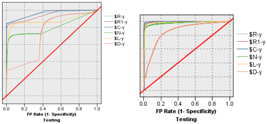
In addition to the confusion-matrix-based metrics described above, the Area Under the Receiver Operating Characteristic Curve (AUC-ROC) was computed for each model. The ROC curve plots the TP rate (sensitivity) against the FP rate (1 − specificity) across all possible classification thresholds, providing a threshold-independent measure of a model’s overall discriminative ability. The AUC summarises the ROC curve as a single scalar value ranging from 0.5 (no discriminative ability, equivalent to random classification) to 1.0 (perfect discrimination). AUC is particularly valuable for imbalanced datasets because, unlike accuracy, it is not influenced by class distribution and assesses the model’s ability to distinguish distressed from healthy companies across the full range of decision thresholds [86]. ROC curves for all models estimated on both the raw and pre-processed datasets, and AUC values are reported in Section 3.

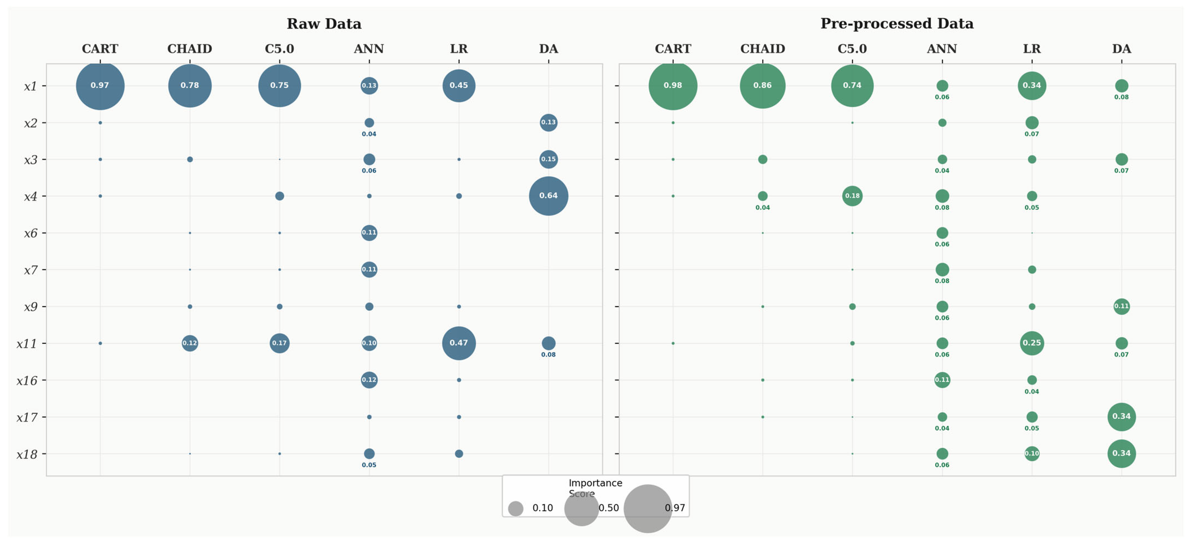
In the Results Section of this study, the details of the individual predictive models are not reported because this research does not aim to propose new predictive models for financial distress. Instead, this study examines and highlights the influence of data preparation on the predictive performance of various modelling techniques. Accordingly, the Results Section presents and compares predictive performance across raw and pre-processed datasets, using confusion matrices and evaluation metrics (10)–(14) for each model. Additionally, to provide insight into the models, we present charts that illustrate the importance of individual predictors for each modelling technique. These charts depict the relative importance of the predictors, with the sum of their importance across all predictors in the study equal to 1.

All calculations were conducted using IBM SPSS Statistics, version 27, and IBM SPSS Modeler, version 18.0. When necessary, a significance level of 0.05 was used for hypothesis testing.

3. Results

The Results Section compares the predictive performance of all modelling techniques estimated on both the raw and pre-processed datasets. The analysis focuses on confusion matrices and key evaluation metrics: accuracy (Acc), sensitivity (Sens), specificity (Spec), precision (Prec), F1 score, and area under the ROC curve (AUC), in order to quantify the impact of data preparation under identical modelling conditions. For each model, predictor importance profiles are also discussed to assess whether data cleaning modifies the financial indicators driving classification decisions. All confusion matrices and evaluation metrics presented below were computed on the held-out testing set.

Table 4 compares the predictive performance and predictor importance of the two CART models using raw versus pre-processed data.

Table 4. Evaluation of prediction performance of CART models.

CART Raw				CART Pre-Processed
	Predicted		%		Predicted		%
Actual	0	1		Actual	0	1
0	27,105	15,626	Spec = 63.43	0	26,217	7	Spec = 99.97
1	2643	87,403	Sens = 97.06	1	2626	71,319	Sens = 96.45
%		Prec = 84.83	Acc = 86.24	%		Prec = 99.99	Acc = 97.37

Source: own elaboration (2026).

Table 4. Evaluation of prediction performance of CART models.

CART Raw				CART Pre-Processed
	Predicted		%		Predicted		%
Actual	0	1		Actual	0	1
0	27,105	15,626	Spec = 63.43	0	26,217	7	Spec = 99.97
1	2643	87,403	Sens = 97.06	1	2626	71,319	Sens = 96.45
%		Prec = 84.83	Acc = 86.24	%		Prec = 99.99	Acc = 97.37

Source: own elaboration (2026).

The results in Table 4 indicate that data preparation leads to a pronounced improvement in CART performance. The model trained on raw data achieves an accuracy of slightly over 86%, whereas the model estimated on pre-processed data achieves slightly over 97%, representing a substantial gain in overall classification accuracy. This improvement is driven primarily by a dramatic increase in specificity, rising from nearly 64% to almost 100%, indicating a near-complete elimination of false-positive classifications of financially healthy companies, with the number of false positives decreasing from more than 15,600 to just 7. From an economic perspective, this is highly significant: in the raw-data model, a large share of financially healthy companies would be incorrectly flagged as distressed, potentially triggering unwarranted credit restrictions or restructuring interventions. The pre-processed model effectively resolves this problem, making its distress signals far more reliable in practice. Sensitivity remains high in both cases, decreasing only marginally from slightly over 97% to slightly under 97%, indicating that the improvement in overall accuracy is achieved by substantially better discrimination of healthy companies while preserving strong detection of distressed ones. Precision increases from nearly 85% to almost 100%, reflecting the near-elimination of false positives and confirming that almost every company labelled as distressed in the cleaned dataset is genuinely at risk. The F1 score increases from slightly over 90% to slightly over 98%, indicating that the pre-processed-data model achieves a more consistent and balanced performance overall. This conclusion is further supported by the AUC, which increases from 0.95 for the raw data model to 0.98 for the pre-processed data model, confirming an improvement in the model’s overall discriminative ability across classification thresholds.

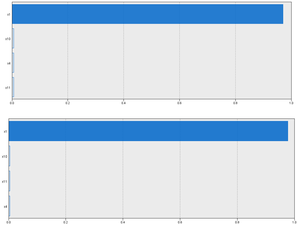
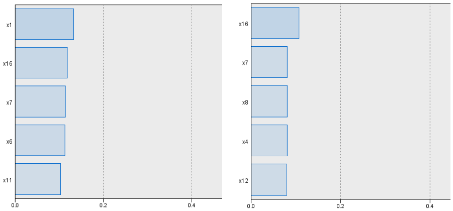
Figure 1 illustrates predictor importance for both CART models. The upper panel belongs to the CART model developed on the raw data, whereas the lower panel corresponds to the model developed on the pre-processed data.

Figure 1. Importance of predictors in CART models. Source: own elaboration (2026).

Figure 1. Importance of predictors in CART models. Source: own elaboration (2026).

In both the raw and pre-processed datasets, cash ratio (x1) is by far the most influential predictor, with all remaining variables contributing only marginally to the tree’s decisions. This strong dominance of a single liquidity indicator suggests that CART relies on a small number of highly discriminative split rules centred on immediate payment capacity, and that these rules become substantially more effective once data imperfections are removed. Taken together, the results imply that CART is highly sensitive to data imperfections: when applied to uncleaned inputs, the model generates numerous false alarms for healthy companies, whereas cleaning and economic validation stabilise the splitting process and enable the tree to separate healthy and distressed companies far more reliably.

Table 5 presents the confusion matrices and evaluation metrics for CHAID models trained on raw and pre-processed data.

Table 5. Evaluation of prediction performance of CHAID models.

CHAID Raw				CHAID Pre-Processed
	Predicted		%		Predicted		%
Actual	0	1		Actual	0	1
0	40,968	1763	Spec = 95.87	0	25,470	754	Spec = 97.12
1	14,614	75,432	Sens = 83.77	1	2243	71,702	Sens = 96.97
%		Prec = 97.72	Acc = 87.67	%		Prec = 98.96	Acc = 97.01

Source: own elaboration (2026).

Table 5. Evaluation of prediction performance of CHAID models.

CHAID Raw				CHAID Pre-Processed
	Predicted		%		Predicted		%
Actual	0	1		Actual	0	1
0	40,968	1763	Spec = 95.87	0	25,470	754	Spec = 97.12
1	14,614	75,432	Sens = 83.77	1	2243	71,702	Sens = 96.97
%		Prec = 97.72	Acc = 87.67	%		Prec = 98.96	Acc = 97.01

Source: own elaboration (2026).

The results in Table 5 indicate a substantial improvement in predictive performance after data preparation. Overall accuracy increases from nearly 88% for the raw-data model to slightly over 97% for the pre-processed-data model. Unlike the pattern observed with CART, the primary driver of this improvement is a pronounced increase in sensitivity, rising from nearly 84% to almost 97%, indicating a considerable reduction in missed distress cases—false negatives decrease from more than 14,600 to slightly over 2200. This is economically important: the raw-data CHAID model fails to identify many genuinely distressed companies, posing a serious risk to creditors, investors, and other stakeholders who rely on the model’s predictions to support their decisions. The pre-processed model reduces this risk substantially by capturing a much higher proportion of truly distressed firms. At the same time, specificity improves modestly, from nearly 96% to slightly over 97%, reflecting a further reduction in false alarms among healthy companies, with false positives decreasing from slightly over 1700 to slightly under 800. Precision increases from nearly 98% to almost 99%, and the F1 score rises markedly from slightly over 90% to nearly 98%, confirming that the pre-processed-data model achieves substantially stronger, more balanced overall performance in identifying distressed firms while keeping false distress signals low. A similar pattern can be observed in the AUC, which rises from 0.94 for the raw data model to 0.97 for the pre-processed model, further underscoring the stronger discriminative performance achieved after data preparation.

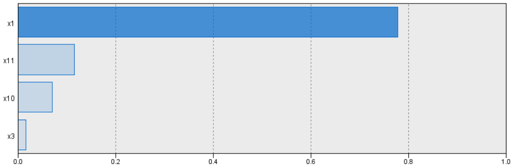
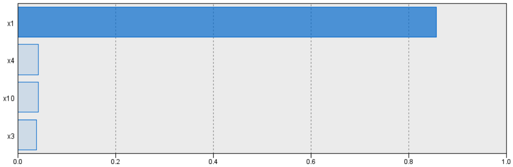
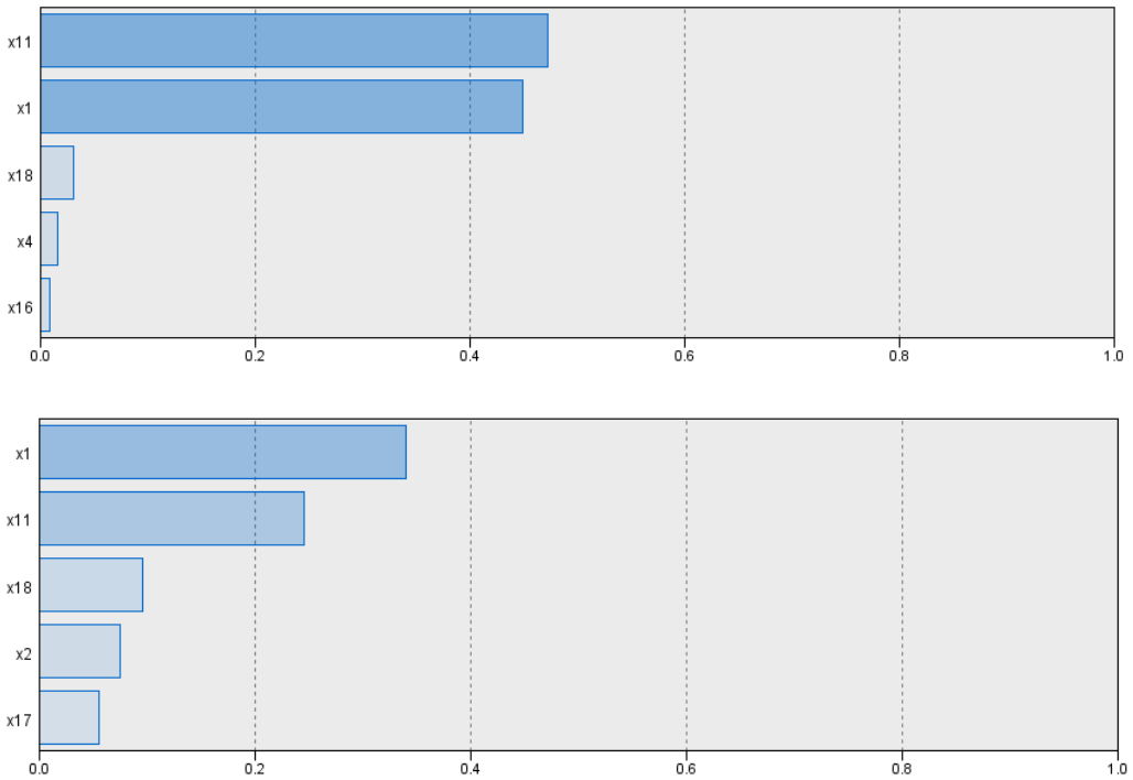
Figure 2 illustrates predictor importance for the most important predictors in the CHAID models, where the upper panel corresponds to the model estimated on raw data and the lower panel to the model estimated on pre-processed data.

Figure 2. Importance of predictors in CHAID models. Source: own elaboration (2026).

Figure 2. Importance of predictors in CHAID models. Source: own elaboration (2026).

In both datasets, cash ratio (x1) remains the most influential predictor by a wide margin, confirming the central role of immediate liquidity in tree-based classification. Beyond this leading variable, the raw-data model assigns relatively greater importance to leverage and capital-structure measures, most notably total debt to equity (x11) and equity ratio (x10), while current ratio (x3) plays only a minor role. In contrast, in the pre-processed-data model, total debt ratio (x4) emerges as the second most influential predictor, while equity ratio (x10) remains among the contributing variables with a smaller relative weight. This shift suggests that data preparation affects how CHAID allocates importance across financial indicators, likely by removing noise and economically implausible values that distort the model’s splitting criteria in the raw data, allowing indebtedness measures to emerge more clearly as discriminative signals.

Table 6 presents the confusion matrices and evaluation metrics for the C5.0 decision tree models trained on raw and pre-processed data.

Table 6. Evaluation of prediction performance of C5 models.

C5.0 Raw				C5.0 Pre-Processed
	Predicted		%		Predicted		%
Actual	0	1		Actual	0	1
0	25,381	17,350	Spec = 59.40	0	25,876	348	Spec = 98.67
1	1307	88,739	Sens = 98.55	1	1515	72.43	Sens = 97.95
%		Prec = 83.65	Acc = 85.95	%		Prec = 99.52	Acc = 98.14

Source: own elaboration (2026).

Table 6. Evaluation of prediction performance of C5 models.

C5.0 Raw				C5.0 Pre-Processed
	Predicted		%		Predicted		%
Actual	0	1		Actual	0	1
0	25,381	17,350	Spec = 59.40	0	25,876	348	Spec = 98.67
1	1307	88,739	Sens = 98.55	1	1515	72.43	Sens = 97.95
%		Prec = 83.65	Acc = 85.95	%		Prec = 99.52	Acc = 98.14

Source: own elaboration (2026).

The results in Table 6 show a pronounced improvement in predictive performance after data preparation, broadly consistent with the pattern observed for CART. Accuracy increases from nearly 86% for the raw-data model to slightly over 98% for the pre-processed-data model. This improvement is driven mainly by a dramatic increase in specificity, which rises from nearly 60% to almost 99%, reflecting a near-elimination of false-positive classifications of healthy companies, where the false positives decreased from more than 17,300 to just under 350. As with CART, the economic implication is significant: the raw-data C5.0 model generates a large number of false alarms for healthy firms, which would undermine the practical utility of the model in credit risk assessment and financial monitoring. After data preparation, this problem is effectively resolved. Sensitivity remains very high in both cases, decreasing only slightly from nearly 99% to slightly under 98%, indicating that the model retains a strong ability to detect genuinely distressed firms after cleaning, though it misses marginally more distressed cases (false negatives increase slightly from slightly over 1300 to slightly over 1500). Precision improves from nearly 84% to slightly over 99%, and the F1 score increases from slightly over 90% to nearly 99%, reflecting that the pre-processed-data model produces far more reliable distress classifications while maintaining near-perfect detection performance. This positive shift is also evident in the AUC, which increases from 0.96 for the raw data model to 0.99 for the pre-processed data model, highlighting the excellent discriminative capacity of the cleaned data specification.

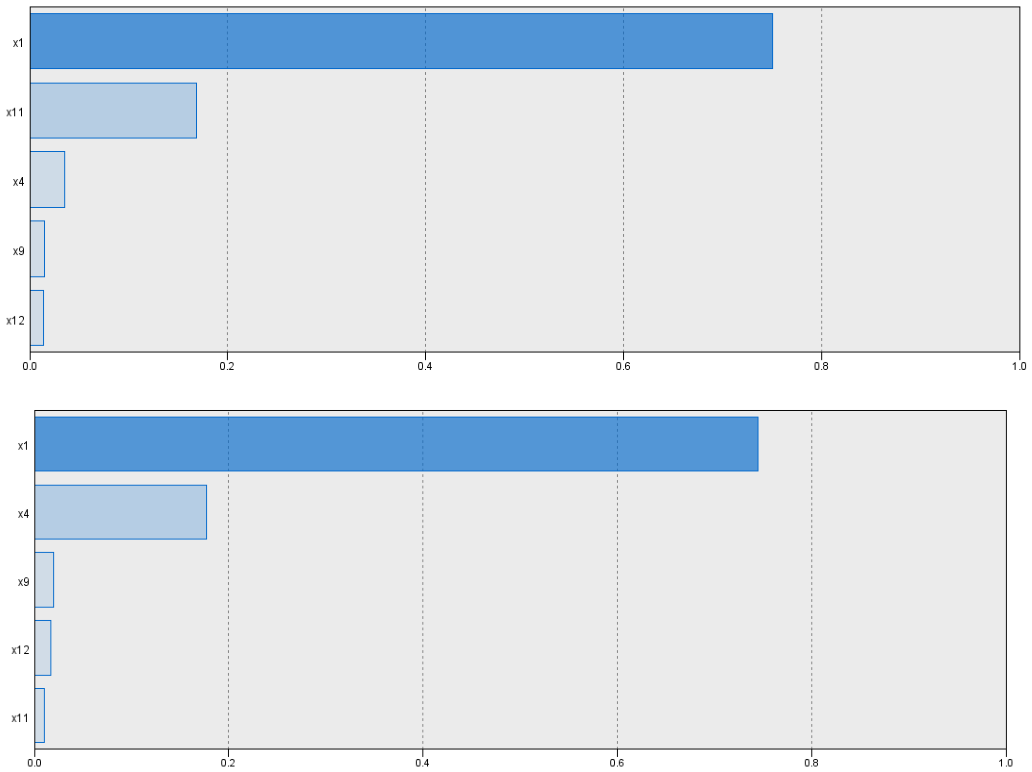
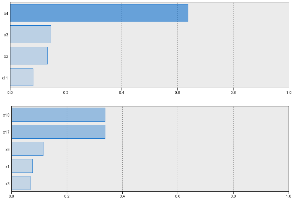
Figure 3 illustrates the predictor importance of the most important predictors in the C5.0 models, where the upper panel corresponds to the model estimated on raw data and the lower panel to the model estimated on pre-processed data.

Figure 3. Importance of predictors in C5 models. Source: own elaboration (2026).

Figure 3. Importance of predictors in C5 models. Source: own elaboration (2026).

Cash ratio (x1) remains by far the most influential predictor in both datasets, while the contribution of the remaining variables is comparatively smaller. In the raw-data model, the second most important variable is total debt to equity (x11), followed by total debt ratio (x4), with short-term payables turnover period (x9) and financial leverage (x12) contributing only marginally. After pre-processing, the ranking among secondary predictors changes: total debt ratio (x4) becomes the clear second most influential variable, while total debt to equity (x11) drops out of the top contributors and is replaced by short-term payables turnover period (x9). This shift suggests that data cleaning makes the importance structure more economically consistent, enabling the model to rely more on fundamental solvency and payment-discipline indicators rather than leverage ratios that may be distorted by extreme or implausible values in the raw data.

Table 7 presents the confusion matrices and evaluation metrics for the ANN models trained on both raw and pre-processed data.

Table 7. Evaluation of the prediction performance of ANN models.

ANN Raw					ANN Pre-Processed
	Predicted		Unpredicted	%		Predicted		%
Actual	0	1			Actual	0	1
0	12,597	3921	26,213	Spec = 29.48	0	24,633	1591	Spec = 93.93
1	1371	64,118	24,557	Sens = 71.21	1	4257	69,688	Sens = 94.24
%		Prec = 94.24		Acc = 57.78	%		Prec = 97.77	Acc = 94.16

Source: own elaboration (2026).

Table 7. Evaluation of the prediction performance of ANN models.

ANN Raw					ANN Pre-Processed
	Predicted		Unpredicted	%		Predicted		%
Actual	0	1			Actual	0	1
0	12,597	3921	26,213	Spec = 29.48	0	24,633	1591	Spec = 93.93
1	1371	64,118	24,557	Sens = 71.21	1	4257	69,688	Sens = 94.24
%		Prec = 94.24		Acc = 57.78	%		Prec = 97.77	Acc = 94.16

Source: own elaboration (2026).

The results in Table 7 reveal the most dramatic performance improvement across all modelling techniques. ANN accuracy increases from slightly under 58% on raw data to slightly over 94% on pre-processed data. The raw-data ANN model is severely compromised by the presence of a large number of unpredicted cases, with more than 26,000 for healthy companies and nearly 25,000 for distressed companies, reflecting the model’s inability to process observations containing economically implausible values or extreme inputs. This failure to produce predictions for a substantial share of the test set has direct practical consequences: in a real-world application, such a model would be unable to assess a large proportion of companies, severely limiting its operational usefulness. After data preparation, no unclassified cases occur, indicating that the preprocessing resolves the input incompatibility that prevented the ANN from functioning reliably on the raw data.

The most notable individual improvement after preprocessing is observed in specificity, which increases from slightly under 30% to nearly 94%, reflecting a sharp reduction in false-positive classifications of healthy companies. From an economic standpoint, a specificity of under 30% in the raw-data model means that roughly seven out of ten financially healthy companies would be incorrectly identified as distressed—an outcome that would render the model practically unusable for credit assessment or regulatory monitoring. Sensitivity also improves substantially, rising from slightly over 71% to slightly over 94%, indicating that the pre-processed model identifies a much higher proportion of genuinely distressed firms. Precision increases from slightly over 9% to nearly 98%, and the F1 score improves substantially from approximately 70% to around 96%, indicating that preprocessing significantly enhances the balance between precision and recall. This suggests that the observed performance gains are driven not only by improved class separation, reflected in higher specificity and sensitivity, but also by a more consistent and reliable identification of both classes. The same development is reflected in the AUC, which rises from 0.80 for the raw data model to 0.98 for the pre-processed model, pointing to a very substantial improvement in overall classification quality across decision thresholds.

Figure 4 illustrates the importance of the most important financial ratios used as predictors in these ANN models, where the left panel shows the model estimated on raw data and the right panel on pre-processed data.

Figure 4. Importance of predictors in ANN models. Source: own elaboration (2026).

Figure 4. Importance of predictors in ANN models. Source: own elaboration (2026).

The predictor importance rankings differ noticeably between the two models. In the raw-data model, cash ratio (x1) and net return on assets (x16) are among the most influential variables, with accounts receivable turnover period including accruals (x7) and total debt to equity (x11) also contributing. In contrast, the pre-processed model places greater emphasis on profitability and receivables management, with net return on assets (x16) becoming the leading predictor, followed by accounts receivable turnover period, including accruals (x7) and accounts short-term receivable turnover period including accruals (x8). The disappearance of the cash ratio (x1) from the top predictors in the pre-processed ANN model is noteworthy and suggests that, once implausible liquidity values are removed, the network can identify more nuanced patterns in profitability and receivables behaviour as the primary signals of financial distress. This redistribution of importance confirms that data preparation not only improves ANN performance but also fundamentally alters the model’s internal structure and the financial mechanisms it captures.

Table 8 presents the confusion matrices and evaluation metrics for the LR models trained on raw and pre-processed data.

Table 8. Evaluation of prediction performance of LR models.

LR Raw				LR Pre-Processed
	Predicted		%		Predicted		%
Actual	0	1		Actual	0	1
0	17,114	8102	Spec = 40.05	0	15,618	10,606	Spec = 59.56
1	732	76,885	Sens = 85.38	1	762	73,183	Sens = 98.97
%		Prec = 90.47	Acc = 70.79	%		Prec = 87.34	Acc = 88.65

Source: own elaboration (2026).

Table 8. Evaluation of prediction performance of LR models.

LR Raw				LR Pre-Processed
	Predicted		%		Predicted		%
Actual	0	1		Actual	0	1
0	17,114	8102	Spec = 40.05	0	15,618	10,606	Spec = 59.56
1	732	76,885	Sens = 85.38	1	762	73,183	Sens = 98.97
%		Prec = 90.47	Acc = 70.79	%		Prec = 87.34	Acc = 88.65

Source: own elaboration (2026).

The results in Table 8 show that LR benefits from data preparation primarily through a substantial improvement in its ability to identify distressed companies. Accuracy increases from slightly over 70% in the raw-data model to nearly 89% in the pre-processed-data model, while sensitivity rises markedly from slightly over 85% to nearly 99%, indicating that the cleaned model captures almost all genuinely distressed firms and misses very few (false negatives increase only marginally from slightly over 730 to slightly under 770). From an economic perspective, this improvement in sensitivity is particularly valuable, as undetected financial distress represents a critical failure in early-warning systems: one that can lead to material losses for creditors and other stakeholders who rely on timely signals.

However, LR exhibits a distinct pattern compared to the tree-based models and ANN: specificity remains relatively low even after preprocessing, improving only from slightly over 40% to nearly 60%. This indicates that a substantial share of financially healthy companies remains classified as distressed. Indeed, false positives increase from slightly over 8100 to slightly over 10,600 after cleaning, suggesting that LR becomes more inclined to predict the distressed class following preprocessing, likely due to the oversampling applied to the training set, which shifts the decision boundary towards the distressed class. This tendency is reflected in a decrease in precision from slightly over 90% to slightly over 87% and a slight decline in the F1 score from slightly under 95% to slightly under 93%. Taken together, these results suggest that while data preparation enhances LR’s sensitivity and overall accuracy, the model’s inherent structural limitations, particularly its linear decision boundary and distributional assumptions, constrain its ability to achieve a well-balanced separation between healthy and distressed companies, even when input data quality is substantially improved. This is also visible in the AUC, which increases from 0.87 for the raw data model to 0.98 for the pre-processed model, indicating a substantial improvement in overall discriminative ability despite the persistence of weaker specificity. Taken together, these findings imply that data preparation strengthens LR mainly by improving its capacity to identify distressed firms, but its structural characteristics, especially the linear decision boundary and underlying distributional assumptions, still limit its ability to cleanly distinguish between healthy and distressed companies.

Figure 5 illustrates predictor importance for the LR models, where the upper panel corresponds to the model estimated on raw data and the lower panel to the model estimated on pre-processed data.

Figure 5. Importance of predictors in LR models. Source: own elaboration (2026).

Figure 5. Importance of predictors in LR models. Source: own elaboration (2026).

In the raw-data model, the highest importance is assigned to total debt to equity (x11) and cash ratio (x1), indicating that the model is driven primarily by leverage structure and immediate liquidity, while the remaining predictors—net return on equity (x18), total debt ratio (x4), and net return on assets (x16)—contribute only marginally. In the pre-processed LR model, the ranking changes: cash ratio (x1) becomes the dominant predictor, followed by total debt to equity (x11), with the set of secondary contributors expanding to include net return on equity (x18), quick ratio (x2), and gross return on equity (x17). These importance profiles should be interpreted with caution given the still-low specificity of both LR models: the reported importance partly reflects the model’s tendency to classify a large share of firms as distressed rather than a genuinely balanced discrimination between healthy and distressed companies.

Similarly, Table 9 presents a comparison of prediction performance between the two models developed using the DA method.

Table 9. Evaluation of prediction performance of DA models.

DA Raw				DA Pre-Processed
	Predicted		%		Predicted		%
Actual	0	1		Actual	0	1
0	283	42,448	Spec = 0.66	0	284	25,940	Spec = 1.08
1	890	89,156	Sens = 99.01	1	258	73,687	Sens = 99.65
%		Prec = 67.75	Acc = 67.36	%		Prec = 73.96	Acc = 73.85

Source: own elaboration (2026).

Table 9. Evaluation of prediction performance of DA models.

DA Raw				DA Pre-Processed
	Predicted		%		Predicted		%
Actual	0	1		Actual	0	1
0	283	42,448	Spec = 0.66	0	284	25,940	Spec = 1.08
1	890	89,156	Sens = 99.01	1	258	73,687	Sens = 99.65
%		Prec = 67.75	Acc = 67.36	%		Prec = 73.96	Acc = 73.85

Source: own elaboration (2026).

The results in Table 9 indicate that DA performs very poorly at separating financially healthy from distressed companies, primarily due to near-zero specificity across both datasets. In the raw-data model, specificity is well under 1%, meaning that only slightly over 280 financially healthy companies are correctly classified as healthy (true negatives), while more than 42,000 healthy firms are incorrectly labelled as distressed (false positives). Although sensitivity is near-perfect at slightly over 99%, the overall accuracy of slightly over 67% reflects an almost complete inability to distinguish healthy from distressed companies, as the model effectively assigns the distressed label to nearly all observations.

A similarly problematic pattern persists after pre-processing. Sensitivity remains almost perfect at slightly under 100%, and accuracy improves only modestly to slightly under 74%, but specificity rises merely to just over 1%. As a result, only slightly more than 280 healthy companies are correctly identified, whereas nearly 26,000 are still falsely classified as distressed. From a practical perspective, this severely limits the usefulness of the model, since such an excessive number of false alarms would make it unsuitable for credit risk assessment, financial surveillance, or regulatory decision-making. Although the AUC increases from 0.72 for the raw data model to 0.85 for the pre-processed-data model, suggesting better overall ranking performance, this improvement is not sufficiently reflected in the final classification outcomes. Thus, while pre-processing enhances the model’s discriminatory potential to some extent, DA remains ineffective in operational terms. This points to an inherent methodological limitation rather than a problem that can be resolved through better data preparation alone, particularly given the method’s dependence on assumptions such as multivariate normality and equal covariance matrices.

Figure 6 illustrates the predictor importance of the most important predictors in the DA models, where the upper panel corresponds to the model estimated on raw data and the lower panel to the model estimated on pre-processed data.

Figure 6. Importance of predictors in DA models. Source: own elaboration (2026).

Figure 6. Importance of predictors in DA models. Source: own elaboration (2026).

In the raw-data model, the importance profile is strongly concentrated in total debt ratio (x4), which dominates the ranking by a wide margin, with current ratio (x3) and quick ratio (x2) contributing modestly. After pre-processing, the profile shifts markedly towards profitability indicators, with net return on equity (x18) and gross return on equity (x17) becoming the most influential predictors jointly, while short-term payables turnover period (x9) and liquidity ratios play a smaller role. This shift from debt and liquidity dominance in the raw-data model to profitability dominance in the pre-processed model is economically interesting, as it suggests that once implausible debt-related values are removed, DA identifies profitability deterioration as the primary discriminating signal. However, given the near-zero specificity of both models, these importance profiles should be interpreted with considerable caution, as the reported weights largely reflect a model that predicts the distressed class for virtually all observations rather than a model that genuinely discriminates between financially healthy and distressed companies.

To provide an overall comparison across modelling techniques, Figure 7 presents the ROC curves for all models created using the raw data (left side) and pre-processed data (right side).

Figure 7. ROC curves for all models on raw data (left) and pre-processed data (right). Source: own elaboration (2026).

Figure 7. ROC curves for all models on raw data (left) and pre-processed data (right). Source: own elaboration (2026).

To disentangle the contribution of each preprocessing step to the observed performance improvements, Table 10 presents evaluation metrics at each stage of the pipeline: raw data, after Step 1 (economic plausibility screening) only, after Steps 1 and 2 (plausibility screening and missing value imputation), and after all three steps (the fully pre-processed dataset).

Table 10. Comparative evaluation of model performance on raw and pre-processed datasets.

Data	Raw Data						Step 1
Modelling technique	Acc	Sens	Spec	Prec	F1	AUC	Acc	Sens	Spec	Prec	F1	AUC
CART	86.24	97.06	63.43	84.83	90.54	0.95	85.93	97.93	63.12	84.38	90.27	0.95
CHAID	87.67	83.77	95.87	97.72	90.21	0.94	87.6	83.29	96.45	97.97	90.03	0.96
C5.0	85.95	98.55	59.4	83.65	90.49	0.96	85.45	98.59	58.47	82.98	90.11	0.96
ANN	57.78	71.21	29.48	94.24	96.04	0.8	58.04	70.63	32.19	96.47	69.36	0.8
LR	70.79	85.38	40.05	90.47	94.57	0.87	57.23	70.4	30.18	95.18	68.88	0.8
DA	67.36	99.01	0.66	67.75	80.45	0.72	67.17	65.51	62.09	78.44	73.37	0.75
Data	Step 2						Pre-Processed Data
Modelling technique	Acc	Sens	Spec	Prec	F1	AUC	Acc	Sens	Spec	Prec	F1	AUC
CART	97.38	96.46	99.97	99.99	98.19	0.98	97.37	96.45	99.97	99.99	98.19	0.98
CHAID	96.56	96.1	97.85	99.21	97.63	0.99	97.01	96.97	97.12	98.96	97.95	0.97
C5.0	98.28	98.34	98.13	99.33	98.83	0.99	98.14	97.95	98.67	99.52	98.73	0.99
ANN	74.61	82.17	53.41	97.47	82.67	0.86	94.16	94.24	93.93	97.77	95.97	0.98
LR	71.28	80.09	46.59	94.6	80.43	0.85	88.65	98.97	59.56	87.34	92.79	0.98
DA	72.94	98.4	1.6	73.7	84.28	0.93	73.85	99.65	1.08	73.96	84.91	0.85

Source: own elaboration (2026).

Table 10. Comparative evaluation of model performance on raw and pre-processed datasets.

Data	Raw Data						Step 1
Modelling technique	Acc	Sens	Spec	Prec	F1	AUC	Acc	Sens	Spec	Prec	F1	AUC
CART	86.24	97.06	63.43	84.83	90.54	0.95	85.93	97.93	63.12	84.38	90.27	0.95
CHAID	87.67	83.77	95.87	97.72	90.21	0.94	87.6	83.29	96.45	97.97	90.03	0.96
C5.0	85.95	98.55	59.4	83.65	90.49	0.96	85.45	98.59	58.47	82.98	90.11	0.96
ANN	57.78	71.21	29.48	94.24	96.04	0.8	58.04	70.63	32.19	96.47	69.36	0.8
LR	70.79	85.38	40.05	90.47	94.57	0.87	57.23	70.4	30.18	95.18	68.88	0.8
DA	67.36	99.01	0.66	67.75	80.45	0.72	67.17	65.51	62.09	78.44	73.37	0.75
Data	Step 2						Pre-Processed Data
Modelling technique	Acc	Sens	Spec	Prec	F1	AUC	Acc	Sens	Spec	Prec	F1	AUC
CART	97.38	96.46	99.97	99.99	98.19	0.98	97.37	96.45	99.97	99.99	98.19	0.98
CHAID	96.56	96.1	97.85	99.21	97.63	0.99	97.01	96.97	97.12	98.96	97.95	0.97
C5.0	98.28	98.34	98.13	99.33	98.83	0.99	98.14	97.95	98.67	99.52	98.73	0.99
ANN	74.61	82.17	53.41	97.47	82.67	0.86	94.16	94.24	93.93	97.77	95.97	0.98
LR	71.28	80.09	46.59	94.6	80.43	0.85	88.65	98.97	59.56	87.34	92.79	0.98
DA	72.94	98.4	1.6	73.7	84.28	0.93	73.85	99.65	1.08	73.96	84.91	0.85

Source: own elaboration (2026).

The results reveal that the three preprocessing steps contribute unevenly across modelling techniques. For tree-based models—CART, CHAID, and C5.0—missing value imputation (Step 2) accounts for the dominant share of the accuracy gains, contributing more than 95% of the total improvement in each case, while plausibility screening alone (Step 1) produces negligible or marginally negative changes. This pattern reflects the sequential dependency of the pipeline: Step 1 removes implausible observations but does not address incomplete data, leaving models with a cleaner but reduced and still incomplete training set. Step 2 resolves this by replacing missing values with sector-mean imputations, enabling tree-based models to build stable, reliable splitting rules. For ANN and LR, the contribution of class balancing (Step 3) is substantially larger, adding almost 20 and over 17 percentage points of accuracy, respectively—consistent with the well-documented sensitivity of these methods to class imbalance. DA exhibits a distinctive pattern: specificity rises markedly after Step 1 before reverting to near-zero after Step 2, attributable to DA’s treatment of missing values temporarily reducing class imbalance in the effective sample. While specificity remains near zero throughout—rendering the model practically unusable for financial distress detection—AUC improves more meaningfully across the preprocessing stages, rising from 0.72 on raw data to 0.93 after Step 2, before settling at 0.85 in the fully pre-processed dataset. This suggests that data preparation does improve DA’s underlying discriminative ability to some extent, but cannot overcome its fundamental methodological constraints.

To summarise the overall impact of data preparation, the average gain in each evaluation metric was computed for each modelling technique as the difference between its performance on the pre-processed dataset and its performance on the raw dataset, and these differences were then averaged across all six models. On average, overall accuracy increased by approximately 15.6 percentage points, ranging from 6.5 percentage points for DA to 36.4 percentage points for ANN, and specificity increased by approximately 26.9 percentage points following data preparation. At the same time, the variation in accuracy across the six modelling techniques narrowed from nearly 30 percentage points in the raw dataset to slightly above 24 percentage points in the pre-processed dataset.

To complement the performance comparison in Table 10, Table 11 summarises the three most influential predictors identified by each modelling technique for both datasets.

Table 11. Comparison of top predictor rankings by model type for raw and pre-processed datasets.

Data	Modelling Technique	1st Predictor (Importance)	2nd Predictor (Importance)	3rd Predictor (Importance)
Raw data	CART	X1 (0.97)	X10 (0.01)	X4 (0.01)
	CHAID	X1 (0.78)	X11 (0.12)	X10 (0.07)
	C5.0	X1 (0.75)	X11 (0.17)	X4 (0.04)
	ANN	X1 (0.13)	X16 (0.12)	X7 (0.11)
	LR	X11 (0.47)	X1 (0.45)	X18 (0.03)
	DA	X4 (0.64)	X3 (0.15)	X2 (0.13)
Pre-processed data	CART	X1 (0.98)	X10 (0.01)	X11 (0.01)
	CHAID	X1 (0.86)	X4 (0.04)	X10 (0.04)
	C5.0	X1 (0.74)	X4 (0.18)	X9 (0.02)
	ANN	X16 (0.11)	X7 (0.08)	X8 (0.08)
	LR	X1 (0.34)	X11 (0.25)	X18 (0.10)
	DA	X18 (0.34)	X17 (0.34)	X9 (0.11)

Source: own elaboration (2026).

Table 11. Comparison of top predictor rankings by model type for raw and pre-processed datasets.

Data	Modelling Technique	1st Predictor (Importance)	2nd Predictor (Importance)	3rd Predictor (Importance)
Raw data	CART	X1 (0.97)	X10 (0.01)	X4 (0.01)
	CHAID	X1 (0.78)	X11 (0.12)	X10 (0.07)
	C5.0	X1 (0.75)	X11 (0.17)	X4 (0.04)
	ANN	X1 (0.13)	X16 (0.12)	X7 (0.11)
	LR	X11 (0.47)	X1 (0.45)	X18 (0.03)
	DA	X4 (0.64)	X3 (0.15)	X2 (0.13)
Pre-processed data	CART	X1 (0.98)	X10 (0.01)	X11 (0.01)
	CHAID	X1 (0.86)	X4 (0.04)	X10 (0.04)
	C5.0	X1 (0.74)	X4 (0.18)	X9 (0.02)
	ANN	X16 (0.11)	X7 (0.08)	X8 (0.08)
	LR	X1 (0.34)	X11 (0.25)	X18 (0.10)
	DA	X18 (0.34)	X17 (0.34)	X9 (0.11)

Source: own elaboration (2026).

To complement the ranked overview in Table 11, Figure 8 presents the full importance scores visually across all models and both datasets simultaneously. In the bubble plot, only predictors with importance ≥0.09 in at least one model are shown. Bubble size reflects the importance score. The plot allows a direct comparison of the importance structure across modelling techniques and illustrates how data preparation affects the relative contribution of individual predictors to model decisions.

Figure 8. Predictor importance scores across models and datasets. Source: own elaboration (2026).

Figure 8. Predictor importance scores across models and datasets. Source: own elaboration (2026).

In the raw-data models, the importance structure is strongly centred on liquidity and capital-structure measures. Cash ratio (x1) is the leading predictor for CART, CHAID, C5.0, and ANN, while total debt to equity (x11) and equity ratio (x10) repeatedly appear among the most influential variables in the tree-based models. LR is driven mainly by total debt to equity (x11) and cash ratio (x1), suggesting a reliance on leverage and immediate liquidity when models are estimated on uncleaned data. DA stands out as the exception, relying primarily on total debt ratio (x4) alongside liquidity measures, consistent with its tendency to assign excessive weight to highly skewed debt-ratio distributions present in the raw data.

After pre-processing, the relative emphasis shifts towards indebtedness and payment-discipline indicators, particularly within the tree-based models. While cash ratio (x1) remains the dominant predictor for CART, CHAID, and C5.0, total debt ratio (x4) becomes markedly more prominent in CHAID and C5.0, and short-term payables turnover period (x9) enters the top predictors for C5.0. This shift suggests that once implausible liquidity values are removed, the tree-based models are able to identify more structural solvency signals as key discriminating factors. ANN undergoes the most notable transformation: cash ratio (x1) drops out of the top predictors entirely, replaced by net return on assets (x16) as the leading variable and receivables management indicators—accounts receivable turnover period including accruals (x7) and accounts short-term receivable turnover period including accruals (x8)—as secondary contributors. This suggests that the pre-processed ANN captures deteriorating profitability and receivables collection capacity as the primary early-warning signals of financial distress, which is economically meaningful. DA shows the most significant turnaround in predictor structure: in the raw-data model, it relies primarily on debt and liquidity ratios, whereas after cleaning, it shifts towards profitability indicators, with net return on equity (x18) and gross return on equity (x17) dominating, though this shift must again be interpreted cautiously given the near-zero specificity of both DA models.

4. Discussion

The quantitative comparisons summarised in Table 10 allow the relative contribution of data quality and algorithm choice to be assessed directly. The average gain in overall accuracy from preprocessing, calculated as the difference between pre-processed and raw accuracy for each modelling technique, averaged across all six methods, was approximately 15.6 percentage points, ranging from 6.5 percentage points for DA to 36.4 percentage points for ANN. By contrast, the variation in accuracy attributable to algorithm choice was approximately 29.9 percentage points within the raw dataset and 24.3 percentage points within the pre-processed dataset. This suggests that data preparation accounts for roughly one-third of the total performance variation observed across both dimensions combined—a substantial contribution that challenges the prevailing assumption that algorithm selection is the dominant driver of predictive performance. This finding is particularly notable in the context of binary classification, where each observation is assigned to one of two mutually exclusive classes, distressed or non-distressed, and where the distributional properties of the training data interact directly with the decision boundaries learned by each classifier [38,39]. Notably, preprocessing also reduces the variation in performance across algorithms, from 29.9 to 24.3 percentage points, indicating that data quality improvements partially offset the differences between modelling techniques and that all methods benefit from better input data. The effect is particularly pronounced for specificity, with an average gain of approximately 26.9 percentage points, rising from 48.1% on raw data to 75.1% on pre-processed data. Given that data preparation has received far less systematic attention in the financial distress prediction literature than methodological innovation, these figures underscore that improving input data quality is not merely a minor technical adjustment but a primary, underexplored lever for enhancing model reliability.

This finding directly supports the central premise of the “garbage in, garbage out” principle: predictive outcomes are not solely driven by algorithmic sophistication but also by the consistency and economic plausibility of the input data. This principle has been confirmed across a range of classification settings, as Li et al. [43] systematically demonstrate across fourteen real-world datasets that data cleaning meaningfully influences classifier performance. Yet, the direction and magnitude of the improvement depend on the error type, the cleaning method applied, and the classifier used, implying that the relationship between data quality and predictive performance is inherently context-dependent rather than uniformly positive. More broadly, Mohammed et al. [44] empirically confirm across nineteen machine learning algorithms that the quality of training data, measured along dimensions of accuracy, completeness, and consistency, has a substantial impact on model efficiency and reliability, with errors introduced during data collection or aggregation propagating into outputs in ways that are difficult to anticipate. Critically, these broader findings from the machine learning literature are echoed within the financial distress prediction domain itself, as Tsai et al. [39] show that feature selection and data resampling, as core data quality interventions, materially affect binary classification outcomes in financial distress prediction and that their sequencing and combination matter, a finding directly relevant to the present study’s design. A complementary and important question raised by these results concerns the relative contribution of model selection versus data preparation to overall predictive performance, as several recent studies suggest that well-designed preprocessing can enable even standard machine learning models to achieve strong and competitive results without requiring algorithmic complexity. For instance, straightforward ensemble classifiers applied with careful feature engineering and preprocessing have demonstrated robust predictive performance in financial forecasting tasks, suggesting that gains attributed to sophisticated model architectures may sometimes reflect the quality and preparation of the input data rather than inherent algorithmic superiority [88,89]. The quantitative findings reported above provide direct empirical support for this interpretation.

The strongest effects of data preparation are observed for the decision tree models. For CART and C5.0, preprocessing substantially reduces false-positive classifications, resulting in a dramatic increase in specificity while maintaining or improving sensitivity and translating into substantial improvements in overall accuracy. Similar improvements are observed for CHAID, where both sensitivity and overall accuracy increased markedly after data preparation. These results are consistent with earlier studies showing that tree-based methods are highly sensitive to data quality and distributional irregularities. Nyitrai and Virag [50] demonstrate that untreated data artefacts and implausible ratio values can inflate misclassification rates, particularly for healthy companies. The present findings extend this evidence by showing that economically grounded data preparation can stabilise tree structures and significantly improve the balance of classifications without suppressing distress signals. Comparable patterns are also reported in broader credit-risk settings, where feature selection, normalisation, and resampling improve performance across multiple classifiers under scale sensitivity and class imbalance [83].

ANN also benefits markedly from data preparation. In contrast to the raw-data model, which achieves high precision but limited performance on other evaluation metrics, the pre-processed-data ANN achieves not only high precision but also high accuracy, sensitivity, and specificity. This result aligns with empirical findings reported by Aydin et al. [67] and Dube et al. [74], who document that ANN performance in distress prediction is strongly conditioned on the quality and consistency of financial inputs. While ANN is theoretically capable of capturing complex non-linear relationships, its practical effectiveness depends on well-conditioned data, particularly when financial ratios exhibit extreme variability. The improvement observed in this study suggests that preprocessing mitigates noise and scale distortions that otherwise hinder ANN learning. This is consistent with evidence that targeted feature-selection procedures can improve prediction accuracy across several model families, including ANN and decision trees [19].

LR shows more moderate but still meaningful improvements after data preparation. Although all metrics increased substantially, specificity remained relatively low compared to tree-based models and ANN. This pattern is consistent with prior research indicating that LR, while robust and interpretable, struggles with non-linear effects and asymmetric class distributions commonly present in financial distress data [51,79]. The results of the present study confirm that data preparation enhances the predictive capability of logistic models but does not fully overcome their structural limitations in distinguishing distressed from non-distressed firms. It is worth noting, however, that prior studies have demonstrated that logistic regression, when applied to well-prepared data with a carefully selected set of predictors, can achieve competitive binary classification performance without recourse to more complex models, and that the incremental predictive gain from algorithmic complexity may be modest when data quality is high [9]. More broadly, prior work emphasises that preprocessing decisions and validation design can materially shape the apparent robustness of bankruptcy prediction models, particularly for simpler parametric approaches [51].

DA performs poorly in both raw and pre-processed data settings, exhibiting near-perfect sensitivity but extremely low specificity. This behaviour reflects the well-known failure of discriminant methods when distributional assumptions are violated—a common issue in corporate financial ratio datasets, where non-normality and unequal covariance structures are pervasive. Similar findings are reported in earlier comparative studies, where DA tends to overclassify distress when applied to heterogeneous corporate datasets [49]. The negligible improvement in specificity after data preparation confirms that, for this method, data cleaning alone cannot compensate for fundamental methodological constraints.

The detailed analysis provides additional insight into the relative contribution of each preprocessing step to the overall performance improvements. The results reveal a clear pattern: for tree-based models, missing value imputation accounts for the dominant share of the accuracy gains, contributing more than 95% of the total improvement in each case, while plausibility screening alone produces only negligible changes. This reflects the sequential dependency of the pipeline: plausibility screening removes incorrect observations but does not address incomplete data, and it is the subsequent imputation of missing values with economically grounded sector means that enables tree-based models to build stable and reliable splitting rules. For ANN and LR, class balancing emerges as the most impactful step, contributing 19.55 and 17.37 percentage points to accuracy, respectively, consistent with the well-documented sensitivity of these methods to class imbalance. DA follows a distinctive trajectory driven by its internal treatment of missing values, and its AUC improves most substantially after imputation, rising from 0.75 to 0.93, before settling at 0.85 in the fully pre-processed dataset. Taken together, these findings suggest that the relative importance of each preprocessing step is not uniform across methods but depends on the specific sensitivity of each algorithm. Tree-based methods benefit most from complete data, while probability-based and distance-based methods are more sensitive to class distribution. This has practical implications for applied financial distress modelling: rather than applying a one-size-fits-all preprocessing pipeline, practitioners may benefit from tailoring the emphasis of data preparation to the characteristics of the modelling technique employed.

An important aspect of the preprocessing strategy adopted in this study is the distinction between economically incorrect values and extreme but plausible observations. Companies with financially impossible ratio values were excluded as likely reporting errors, while outliers reflecting severe but feasible financial conditions were retained. This approach is consistent with recent methodological recommendations emphasising that extreme ratio values often represent genuine distress dynamics rather than statistical noise [42,50]. The strong performance improvement of most models after preprocessing suggests that preserving economically meaningful extremes contributes to effective early-warning detection, whereas removing incorrect values prevents models from learning artefactual patterns driven by data entry errors or accounting misclassifications rather than actual financial deterioration.

A natural question arising from the magnitude of the observed performance improvements, particularly the near-perfect specificity achieved by tree-based models after preprocessing, is whether these gains partly reflect overfitting induced by the preprocessing procedure itself rather than genuine improvements in predictive validity. This concern deserves explicit consideration. Several features of the study design, however, collectively argue against an interpretation of overfitting induced by preprocessing.

First, and most fundamentally, all performance metrics reported in this study were computed on a held-out test set that was kept strictly separate from the training data and left entirely unmodified throughout the preprocessing and oversampling pipeline. Oversampling was applied exclusively to the training data, and the test set preserves the original, unbalanced class distribution. If the pre-processed models were overfitting to artefacts introduced by the cleaning procedure, this would be expected to manifest as inflated training performance that fails to transfer to the test set. The fact that the improvements in evaluation measures are observed on the held-out test data, not merely on the training set, provides direct evidence against overfitting as the primary explanation for the performance gains. Second, the nature of the preprocessing intervention is important. The approach did not involve smoothing, winsorisation, normalisation, or any transformation that would artificially reduce the variance of the input data or alter the distribution of valid observations. The only modification was the removal of observations with economically impossible ratio values—values that cannot arise from genuinely reported financial data, regardless of the company’s financial condition. Critically, extreme but economically admissible values were deliberately retained, including the heavy-tailed distributions characteristic of financially distressed companies. This is a conservative and information-preserving form of data cleaning that reduces noise without suppressing the genuine signal. Third, the pattern of improvements across methods is consistent with a data-quality-restoration interpretation rather than an overfitting interpretation. Overfitting induced by preprocessing would be expected to inflate performance uniformly across all methods, including those most susceptible to overfitting, such as decision trees. Instead, the observed pattern is heterogeneous: tree-based models benefit primarily through reductions in false positives, LR improves mainly in sensitivity, and DA remains poor despite preprocessing. This method-specific heterogeneity is more naturally explained by the differential sensitivity of each algorithm to the types of data imperfections removed, particularly the elimination of economically implausible values that distorted splitting criteria in tree-based models and caused the ANN to fail entirely on a large share of observations, than by a uniform preprocessing artefact. Fourth, the ANN result provides particularly compelling evidence. In the raw-data setting, the ANN was unable to produce predictions for more than 50,000 observations, which is a fundamental operational failure rather than a modest performance limitation. The improvement after preprocessing, therefore, represents a transition from a non-functional to a functional model, driven by the resolution of input incompatibilities caused by economically implausible and missing values. This pattern cannot plausibly be attributed to overfitting. These considerations together support the interpretation that the observed performance improvements reflect genuine data quality restoration—the removal of noise that was actively misleading the classifiers—rather than artefacts of the preprocessing procedure. Taken together, the results reinforce a broader conclusion from recent literature: preprocessing choices, encompassing feature selection, scaling and normalisation, resampling, and missing-value handling, can systematically improve distress and credit-risk prediction across different algorithm families, not only within a single modelling paradigm [83,90].

Evidence from more complex learners further indicates that carefully designed preprocessing can enhance performance in high-dimensional or otherwise challenging settings, including boosting-based approaches [91] and hybrid feature-selection and ensemble designs [92], while explicitly modelling missingness patterns can improve predictions when missingness is non-random [21]. Complementary work also shows that dedicated imputation and aggregation strategies can increase robustness in datasets affected by missing values [93], and that imbalance and dimensionality issues often require advanced preprocessing to avoid unstable or inflated error rates [17].

It should also be acknowledged that the present study is limited to binary classification of financial distress, in which each firm is assigned exclusively to one of two outcome classes. This design, while standard in the financial distress prediction literature and appropriate for the study’s objectives, does not capture the gradations of financial difficulty that may be relevant in practice, such as early warning stages, temporary liquidity difficulties, or multi-year trajectories toward insolvency. Multi-class or ordinal approaches, as well as survival and hazard-based methods, offer complementary perspectives that binary classifiers cannot provide. The binary framing also means that the evaluation metrics and preprocessing strategies reported here, particularly those related to class imbalance correction, are specific to two-class settings and may require adaptation if the framework is extended to multi-class prediction contexts [37,39].

While the findings provide clear evidence that data preparation substantially influences the predictive performance of financial distress models, several limitations of the study need to be acknowledged. First, the empirical analysis focuses on Slovak companies and on a one-year-ahead prediction horizon. The one-year-ahead prediction horizon is a deliberate and standard methodological choice in financial distress prediction research. The overwhelming majority of studies in this field, from foundational works such as Altman [3] to recent contributions (e.g., [4,24]), adopt a one-year lag between the financial statement date and the distress evaluation year, reflecting both the annual reporting cycle that practitioners rely on and the well-documented decline in predictive power of financial ratios at longer horizons. Although this setting enables a controlled assessment of the effects of data preparation within a homogeneous environment, prior research suggests that prediction performance and variable relevance may vary across countries and economic regimes [9,49]. This introduces a second study limitation concerning cross-country generalisability of the results. The Slovak institutional context has several features that may affect the transferability of the findings. Slovak companies report under a mix of Slovak Accounting Standards and IAS/IFRS, the legal definition of financial distress is grounded in the Slovak Bankruptcy and Restructuring Act, and the sector composition of the dataset reflects the structure of the Slovak economy. These features influence both the distribution of financial ratios and the prevalence and nature of reporting errors and implausible values in the data. It is therefore plausible that the magnitude of preprocessing effects may differ across countries with different accounting frameworks, reporting cultures, and legal definitions of distress. On the other hand, the core argument of this study that economically implausible values distort model performance and that their removal improves predictive accuracy is grounded in the general properties of financial ratio construction rather than in any country-specific feature and is, therefore, expected to hold broadly across institutional contexts. Prior research confirms that prediction performance and variable relevance vary across countries and economic regimes [9,49], and extending the present framework to multi-country datasets would offer valuable insight into whether the magnitude and pattern of preprocessing benefits are stable across different financial systems. Such an extension is identified as a priority direction for future research.

Third, the study employs a comprehensive yet specific data preparation procedure involving economic plausibility checks, missing-value imputation, and class balancing. The strong performance gains observed indicate that such preprocessing is highly effective in this context. At the same time, the recent literature highlights that alternative imputation strategies and imbalance treatments may also lead to complementary improvements [41,42]. Exploring a wider range of preprocessing configurations would further expand best-practice guidelines for applied distress modelling. Additionally, class imbalance was addressed through oversampling in the training data, a widely adopted approach in rare-event prediction. While this technique significantly improved minority-class detection in the current study, future research could compare it with other methods that have shown encouraging results in recent financial applications [16,17], thereby enhancing the robustness of performance conclusions. Next, the modelling framework includes widely used statistical and machine learning techniques but does not cover more recent ensemble approaches, such as boosting and stacking, which often achieve high accuracy in comparable settings [10,92]. Given that the pre-processed models already achieve near-ceiling performance across the key evaluation metrics, the marginal gains that ensemble methods might deliver are expected to be limited in this setting. Nevertheless, including such methods in subsequent research would help assess whether the strong influence of data preparation persists even under more complex predictive architectures.

A related methodological point concerns validation design. The present study employs a single train-test split rather than k-fold cross-validation. This choice is justified on two grounds. First, the dataset is exceptionally large, with more than 130,000 observations in both the training and test sets. At this scale, a single held-out test set provides highly stable and reliable performance estimates; cross-validation is principally designed to address estimation instability in small samples, where a single split would be sensitive to the particular observations assigned to each partition. In the present setting, the statistical reliability of the performance estimates is not in question. Second, the software environment used for model estimation (IBM SPSS Modeler 18.0) does not support k-fold cross-validation for the majority of the classification methods employed in the study, namely CART, CHAID, ANN, LR, and DA. Implementing cross-validation for C5.0 alone while using a train-test split for all other methods would produce an inconsistent evaluation framework across techniques, undermining the direct comparability of results that is central to the study’s design. Finally, replicating the analysis in an open-source environment such as R or Python would allow for greater methodological flexibility, including the implementation of k-fold cross-validation across all modelling techniques and the exploration of a broader range of preprocessing configurations.

Overall, these considerations do not detract from the study’s main contribution but rather delineate promising directions for extending the analysis. The consistent improvements observed across most modelling techniques underscore that rigorous data preparation is a central component of reliable financial distress prediction and should be treated as a substantive methodological stage alongside model selection—one that deserves explicit attention both in empirical research and in the practical deployment of early-warning systems.

5. Conclusions

This study examined the impact of data preparation on the predictive performance of selected statistical and machine learning models in financial distress prediction. By comparing models estimated on raw financial ratio data with models trained on economically pre-processed data, the analysis provides direct empirical evidence on the practical relevance of the “garbage in, garbage out” principle in corporate risk modelling. The results show that data preparation substantially improves predictive performance across most applied methods. The strongest effects are observed with decision tree algorithms (CART, CHAID, and C5.0), in which preprocessing yields a pronounced reduction in false-positive classifications and a significant increase in overall accuracy, while maintaining high sensitivity. ANN also benefits markedly from prepared data, achieving balanced and robust class discrimination after preprocessing. LR exhibits moderate improvement, particularly in sensitivity, although specificity remains limited compared to more flexible methods. DA performs weakly in both settings, indicating that data cleaning alone cannot compensate for restrictive distributional assumptions.

These findings demonstrate that model outputs are not determined solely by the selected algorithm. Instead, they are strongly influenced by how consistently and economically plausibly the input data are prepared. Removing economically implausible financial-ratio values enhances data integrity, while retaining extreme yet feasible observations preserves important distress signals. In this respect, the study confirms that careful preprocessing can yield substantial improvements in predictive performance, with average accuracy gains of approximately 15.6 percentage points across all modelling techniques, amounting to roughly half the performance variation attributable to algorithm choice, thus demonstrating that data quality is a primary determinant of model reliability alongside algorithm selection. A step-level detailed analysis further reveals that the contribution of each preprocessing step is not uniform across methods: missing value imputation accounts for the dominant share of performance gains in tree-based models, while class balancing is the most impactful step for ANN and LR, reflecting the differential sensitivity of each algorithm to data completeness and class distribution, respectively. From a practical perspective, the results highlight that risk assessment systems based exclusively on algorithm optimisation, without systematic attention to data quality, may fail to reach their predictive potential. For practitioners in banking, auditing, and corporate risk management, structured data validation and economically grounded preprocessing should therefore be considered integral components of model development rather than purely technical preliminary steps.

Several directions for future research emerge from this study. First, the analysis could be extended to multi-country datasets to examine whether the magnitude of preprocessing effects differs across institutional and accounting environments. Second, future studies may incorporate additional modelling techniques, particularly ensemble and boosting approaches, to evaluate whether the influence of data preparation persists in more complex predictive architectures. Finally, alternative preprocessing strategies, such as different imputation methods, transformation techniques, or imbalance treatments, could be systematically compared to identify optimal combinations of data cleaning and modelling procedures.

In summary, the study provides empirical support for the view that reliable financial distress prediction depends not only on methodological sophistication but also on disciplined and economically justified data preparation. The evidence suggests that improving data quality is a fundamental step toward developing robust, practically applicable early-warning models.