Assessing Historical and Simulating Future Land-Use and Land-Cover Change Through an Integrated Cellular Automata and Machine-Learning Framework in Urbanizing Areas

Highlights

What are the main findings?

• The CA–ANN model reproduced the observed 2021 LULC map using transition relationships learned from the 2001–2011 period and initialized with the 2011 baseline map, with 90.9% correctness and Kappa = 0.84, accurately capturing the observed spatial distribution of built-up areas near Forney, Terrell, Crandall, and Kaufman, replacing cropland and open areas.
• The model projects an increase of nearly 30% in built-up land by 2051 under the assumed continuation of observed transition dynamics, primarily along the I-20 corridor, U.S. Highway 175, and State Highway 34.

What are the implications of the main findings?

• Corridor-oriented rapid land development on the western and central side of Kaufman County highlights areas where future urban expansion may intersect with agricultural zones and flood-prone corridors such as the Trinity River and Cedar Creek tributaries, indicating the need for targeted zoning and coordinated flood-risk planning.
• The CA–ANN model offers a powerful open-source tool to map suburban expansion hotspots and support land-use planning for fast-growing Texas counties.

Abstract

Rapid urbanization has transformed the face of Texas by converting agricultural and natural lands into expanding built-up areas. This study analyzes and simulates land-use and land-cover (LULC) changes in Kaufman County, Texas, one of the fastest-growing counties in the United States, using a hybrid Cellular Automata–Artificial Neural Network (CA–ANN) model within the Quantum Geographic Information System (QGIS) Modules for Land-Use Change Evaluation (MOLUSCE) framework. Multitemporal NLCD datasets (2001, 2011, and 2021) and six spatial drivers: Elevation, Slope, Aspect, Distance from Roads and Rivers, and Built-up Density were used in the modeling framework. Transition relationships were calibrated using the 2001–2011 LULC data, and the model was validated by simulating the 2021 LULC map from the 2011 baseline. The calibrated model was then used to simulate future LULC scenarios for 2031, 2041, and 2051. Model validation yielded an overall Kappa value of 0.84 and a correctness of 90.9%, indicating high similarity between the observed and simulated maps. The results indicate simulated urban expansion, with built-up areas increasing by nearly 30% by 2051 at the expense of cropland and open areas, with forest and water bodies slightly increasing, and wetlands remaining stagnant. The CA–ANN model effectively captured the nonlinear, spatially dependent land-transition patterns using open-source tools. These findings provided useful information for sustainable land-use planning and environmental management, with the potential to incorporate spatial modeling into regional development strategies in rapidly urbanizing areas of Texas.

1. Introduction

Land-use and land-cover (LULC) transition studies are gaining increasing importance in environmental change research because of accelerated urban growth, rising population, migration, and infrastructure in rapidly urbanizing countries. These processes exert substantial pressure on the natural environment [1,2]. LULC represents both the physical characteristics of the Earth’s surface (land cover) and the human uses that determine its utilization (land use) [3]. The most visible consequence of urbanization is the conversion of agricultural, forest, and wetland areas into urban and built-up lands, leading to significant impacts on ecological integrity [4], food security, water resources, and climate resilience [5]. Remote sensing (RS) and Geographic Information Systems (GIS) tools have become ideal for monitoring and modeling the changes that allow quantification and scenario-based simulation of LULC changes over historical and future periods [2,6,7,8].

Studies have been undertaken in urban areas of the Middle East and South Asia regarding LULC changes and their impacts. From Nepal’s Terai plains [2] and India’s Western Himalayas [9] to conflict-affected Yemen [10] and Iraq’s low folded zone [11], urbanization is one of the most dominant driving factors of landscape change. In Pakistan’s Lahore City, built-up areas increased by more than 300% between 1994 and 2014 [12]. Additionally, in the Kabul River Basin, Afghanistan, urban erosion and vegetation loss have been exacerbated by population and migration pressures [13]. These changes are followed by losses of vegetation, forest, and arable lands, and have consequences for environmental degradation and climate change impacts [14,15,16]. Understanding the implications of these studies, similar studies need to be performed for the United States (US) to quantify the LULC changes for building an understanding of why those changes occurred and what they imply about the future.

Long-term LULC-change studies in the US have played a crucial role in understanding the dynamics of human–environment interactions at various spatial scales. Nationwide-scale programs such as the National Land-Cover Database (NLCD) initiative conducted by the U. S. Geological Survey (USGS) have produced continuous Landsat-based data from 1985 to the present. These tools have shown that agricultural and forested land is rapidly being converted to developed and urban land, particularly in the southeastern states, the Great Plains, and major metropolitan corridors [17,18]. The NLCD 2016 assessment indicated that 5.8% of the conterminous U.S. land cover was developed land, primarily replacing cultivated croplands and deciduous forest land-cover types [17]. Similarly, the Forecasting Scenarios of Land-Use Change (FORE-SCE) model projects that urban expansion will continue through 2100, with the East Coast, Midwest, and West Coast expected to experience the fastest growth [19]. Rapidly growing metropolitan areas in the southeast, such as Atlanta, have some of the fastest rates of built-up growth and significantly increased land surface temperatures [20]. Similar patterns of urbanization and ecological transformation were also seen in Texas, with Landsat-based analysis revealing the rapid conversion of agricultural and prairie land to urbanized land in outlying counties such as Fort Bend (Houston metro), Rockwall (Dallas metro), and Williamson (Austin metro), while central metropolitan counties grew more slowly, and outlying counties expanded extraordinarily, and urbanization moved north. Taken together, these observations showed the ongoing transformation of Texas to a state dominated by an extensive impervious surface and underlain by dwindling vegetation cover [21,22]. Therefore, it becomes crucial to analyze these ongoing transformations and accurately predict future LULC changes to guide sustainable development and informed land-use planning.

The existing literature consistently highlights the socio-economic and environmental effects of unregulated LULC modification. Forest cover losses not only threaten biodiversity but also carbon sequestration, while farmland reductions affect food security. Water scarcity underlies all, with encroachment of watersheds in the Indrayani basin [23] and the Pasighat region [24]. Rapid urban agglomeration expansion in Iraq and India threatens the risk of flooding [25,26,27], pollution, and urban heat islands [6,11]. These studies have reinforced the need for sustainable urban planning and policy intervention in fast-changing, urbanizing countries. The combination of spatial analysis, predictive models, and simulations under different scenarios provides a framework to show how predominant land management trajectories may evolve, and how negative impacts might be averted through evidence-based solutions [1,28]. While many of these documented impacts originate from rapidly urbanizing regions in Asia and the Middle East, similar development pressures are increasingly observed in fast-growing counties in the United States, including parts of Texas.

Traditional models such as Markov Chains, Logistic Regression (LR), Weights of Evidence (WoE), and Conversion of Land Use and Its Effects at Small Regional Extent (CLUE-S) have been used for LULC prediction with drawbacks. Markov models account for the time probability but not the spatial interaction between neighboring pixels. LR and WoE models assume linearity and cannot capture the complex, nonlinear relationship between land transitions and multiple drivers [11]. CLUE-S and SLEUTH are spatial models with numerous calibration parameters, resulting in high computational costs [29,30]. In contrast, the Cellular Automata–Artificial Neural Network (CA–ANN) model integrates CA’s spatial diffusion mechanism with ANN-based transition potential modeling, where the ANN learns nonlinear relationships during calibration and applies them to different spatial driver configurations during simulation, thereby providing strong agreement with observed historical patterns and spatially coherent simulation patterns [31,32]. CA captures the spatial contiguency, which models the state of each cell inferred from the states of neighborhood cells, while ANN learns nonlinear relationships between driving variables (such as elevation, slope, distance to roads, distance to rivers, and built-up density) and is capable of generating spatially coherent future land-transition scenarios under specified assumptions. ANN utilizes nonlinear learning to capture the complex relationships between driving variables and land transitions, while cellular automata introduce spatial feedback that mimics real neighborhood growth and fragmentation. It is highly flexible and scalable, can handle various datasets and scales, has demonstrated strong predictive agreement with observed historical LULC patterns in various empirical applications, and is user-friendly. It can be easily implemented through the Modules for Land-Use Change (MOLUSCE) plugin in Quantum Geographic Information System (QGIS), providing an open-source, user-friendly, interpretable, and reproducible modeling framework without complex coding.

The recent studies reviewed in the literature demonstrated the effectiveness of the CA–ANN in varied climates. In Tellippalai, Sri Lanka, Saha (2024) [33] presented 91% of accuracy and a Kappa = 0.89 for built-up expansion predictions. Kumari & Roy (2025) [9] implemented the same method in the Western Himalayas and validated it with 82% accuracy for long-term projections to 2055. Similarly, the Mand catchment in India used MOLUSCE to simulate the LULC change in India; the Kappa value was around 0.88 and could map the land change trends, such as settling in the area. In the same way, CA–ANN models showed > 90% correctness for the Low Folded Zone, Iraq [11] and 0.86–0.91 Kappa in Malaysia’s Perak River Basin [34]. Although the integrated CA–ANN model has emerged as a dominant theme in the recent literature, the individual components of the Neural Network and Cellular Automaton have been separately validated as effective tools in land-use modeling, specifically in the United States of America. For example, Pijanowski et al. [35] used an ANN-based Land Transformation Model (LTM) to simulate the urban growth processes at the national level, which proved that machine-learning techniques outperform traditional statistical techniques in dealing with the high-dimensional data of the National Land-Cover Database (NLCD). Supporting this, Sun et al. [36] used a CA model to map the spatial processes of rapid expansion in Orange County, Florida, which was effective in dealing with the issue of suburbanization in the region. Most recent work by Vahid and Aly [37] used an integrated CA-Markov model to simulate the land-use changes in the state of Arkansas, USA, which resulted in a maximum Kappa coefficient of 0.90. These models have emerged as the empirical basis of using a hybrid stochastic model coupled with a neural network approach. The applicability of this framework is supported by structural similarities between these U.S. case studies and Kaufman County, which exhibits comparable exurban expansion and agricultural land conversion along major transportation corridors of the Dallas–Fort Worth metropolitan region. Furthermore, the county-scale analysis at 30 m resolution and the driver variables used, including proximity to roads, slope, and elevation, are consistent with those applied in previous LULC simulations. By integrating these two effective techniques into a single CA–ANN model, this study aims to capture both the nonlinear transition probabilities and the spatial growth patterns characteristic of the American landscape.

While the application of CA–ANN models has been extensively implemented for projecting the dynamics of LULC changes across various global regions, the majority of the research has focused on regional scales or environmentally sensitive landscapes. Recent applications of the model across the United States, such as Mehla and Jagadish (2025) [32], have also demonstrated the performance of the model across broader spatial scales. However, the analysis of the dynamics of land transitions across the county level, especially for the rapidly expanding suburban fringe landscapes, has not been extensively addressed by the existing research. Kaufman County was selected for the analysis due to the sustained rates of population expansion and built-up land growth observed over the past two decades. According to U.S. Census Bureau population estimates [38], the county experienced a 36.1% population increase between 2020 and 2024, making it one of the fastest-growing counties in Texas, while NLCD data indicate a substantial increase in built-up land between 2001 and 2021, consistent with metropolitan fringe expansion along the Dallas–Fort Worth corridor [39,40]. The county is representative of the metropolitan fringe, providing an ideal setting for the analysis of corridor effects on the dynamics of land transitions across the county level. The analysis is based on the application of consistent multi-temporal NLCD data (30 m resolution) for the period 2001–2021, along with the simulation of scenarios for the period 2021–2051. This study provides a scale-specific assessment of the magnitude and spatial distribution of land conversion associated with suburban growth. These findings offer spatially explicit evidence of where and how suburban expansion is projected to occur within the county that can support land-use planning discussions related to growth management, agricultural land preservation, and infrastructure development at the county scale. The overall aim of this study is to assess land-transition dynamics and evaluate future suburban expansion patterns at the county scale to support spatial planning in rapidly urbanizing regions. The objectives of the present study are as follows:

• Analyze and quantify the spatiotemporal land-use and land-cover (LULC) changes in Kaufman County, Texas, from 2001 to 2021 using NLCD datasets.
• Identify and evaluate key spatial drivers: elevation, slope, aspect, distance to roads and rivers, and built-up density that influence LULC transitions.
• Simulate future LULC scenarios for 2031, 2041, and 2051 using the CA–ANN model within the QGIS MOLUSCE framework.

2. Materials and Methods

2.1. Study Area

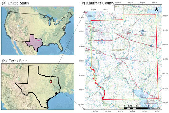
Kaufman County, Texas, is located in the eastern part of the Dallas–Fort Worth metropolitan area. It covers an area of about 808 square miles (i.e., about 2090 km²), of which 781 square miles are land, and it is surrounded by Dallas, Rockwall, Hunt, Van Zandt, Henderson, and Ellis counties (Figure 1). It includes the fast-growing cities of Forney, Terrell, Kaufman, and Crandall. Kaufman County lies in the southern part of the Blackland Prairie [41] and is relatively flat to gently rolling, with elevations ranging 300–550 feet. The land is primarily drained by the East Fork of the Trinity River and its tributaries in the west and by Cedar Creek and its tributaries that feed Cedar Creek Reservoir in the south. Flood-prone areas exist along major channels and low-lying areas. The climate is humid subtropical with hot summers and mild winters; typical July temperatures range from about 72 to 97 °F, and typical January temperatures range from about 33 to 54 °F. The mean annual precipitation is near 39 inches. These conditions support prairie grasslands, riparian woodlands, and agriculture. However, the spread of impervious cover increases the runoff sensitivity [42]. Transportation corridors such as I-20 and US-175 connect the county to regional job centers and have guided suburban growth. This accessibility is reflected in its rapid growth. According to Census-based reporting, the county was the fastest-growing county in Texas [43] and has continued to experience rapid population growth in recent years, reinforcing its relevance as a representative suburban fringe case. Hydrologically, the East Fork of the Trinity River [44] is monitored near Forney and Crandall, highlighting a need for dynamic flood risk management [45] along the main stem and tributaries through rapidly urbanizing areas.

Figure 1. Location map of Kaufman County, Texas: (a) Continental USA showing the position of Texas State, (b) Texas State highlighting Kaufman County, and (c) Detailed map of Kaufman County, with the red boundary representing the study area.

2.2. Data Collection and Preparation

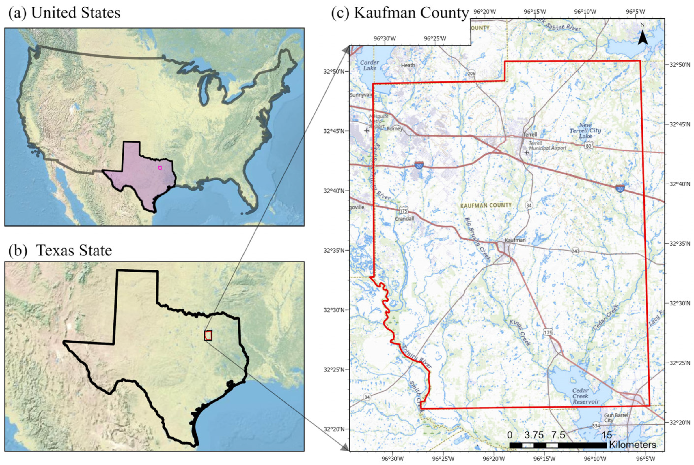
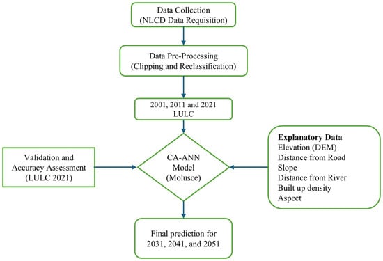
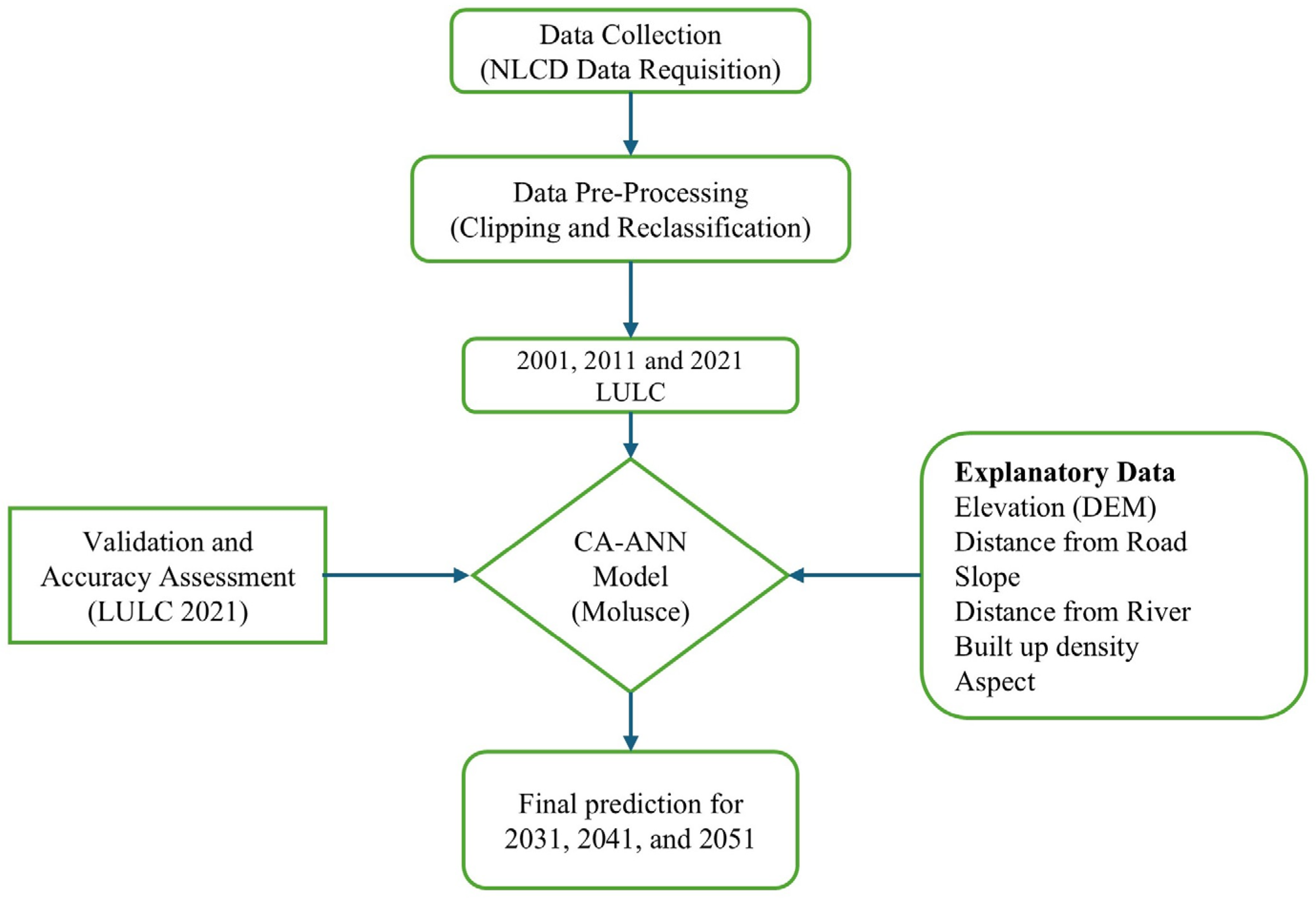
Spatial datasets used in this study were compiled from authoritative open-access sources and were processed to ensure spatial consistency and analytical reliability. The data types used in this research, along with their sources, are provided in Table 1. The National Land-Cover Database (NLCD) from the Multi-Resolution Land Characteristics (MRLC) consortium provided LULC maps for 2001, 2011, and 2021 at 30 m spatial resolution. The Digital Elevation Model (DEM) was obtained from the SRTM 1 Arc Second Global dataset and used to obtain slope and aspect maps. Road networks were obtained from the TIGER Line database of the U.S. Census Bureau, corresponding to data for 2001–2011 training, 2021 validation, and future projection. River networks were extracted from the National Hydrography Dataset Plus (NHDPlus). The creation of distance-from-road and distance-from-river layers was achieved by using Euclidean distance extraction from ArcGIS Pro 3.5.0. Built-up density was created from the Euclidean distance extraction with an 11 × 11 cell (330 m × 330 m) moving-window method. All datasets were projected to NAD 1983 StatePlane Texas North Central FIPS 4202 (Meters), resampled at 30 m, and clipped to the Kaufman County boundary before integration into the model. The 2001 and 2011 LULC maps were used to train the CA–ANN model (using the MOLUSCE plugin version 5.1.0 in QGIS 3.42.3-Münster), and this was achieved through the capture of the observed land-cover transitions from 2001 to 2011 using explanatory variables of 2001. For the model validation, the CA–ANN model was initialized using the 2011 LULC map and the corresponding static and dynamic spatial drivers. One CA iteration was used to simulate the 2021 LULC map. The simulated 2021 LULC map was then validated against the observed 2021 NLCD dataset, and the accuracy of the model was determined. After the validation of the model, future LULC maps were simulated for 2031, 2041, and 2051 using the 2021 spatial drivers as the baseline condition. The projection years (2031, 2041, and 2051) were selected to align with regional planning cycles and ensure CA–ANN mathematical consistency. Specifically, 2031 captures the first policy updates following the 2030 U.S. Census, while 2051 allows for a post-implementation assessment of the North Central Texas Council of Governments (NCTCOG) Mobility 2050 Plan. This ensures the simulation is synchronized with the administrative benchmarks used for infrastructure development in Kaufman County. Maintaining these 10-year decadal intervals preserves the integrity of the transition probability matrix by matching the historical training steps and preventing temporal scaling errors. Figure 2 provides the schematic representation of the methodology used in this research.

Table 1. Datasets used in this study, along with their resolution/Feature type, and Sources.

Sr. No	Parameter	Datasets Used	Spatial Resolution/Feature Type	Source
1	Land-Use and Land-Cover (LULC)	National Land-Cover Database (NLCD) from the Multi-Resolution Land Characteristics (MRLC) Consortium	30 m Raster	https://www.mrlc.gov/ (accessed on 30 September 2025)
2	Digital Elevation Model (DEM)	SRTM 1-Arc Second Global	30 m Raster	https://earthexplorer.usgs.gov/ (accessed on 29 September 2025)
3	Road Network	Topologically Integrated Geographic Encoding and Referencing System (TIGER)	Line Vector	https://www.census.gov/geographies/mapping-files/time-series/geo/tiger-line-file.html (accessed on 30 September 2025)
4	River	National Hydrography Dataset Plus (NHDPlus)	Line Vector	https://apps.nationalmap.gov/downloader/ (accessed on 7 October 2025)
5	Distance from Road	Calculated from Road Network	30 m Raster
6	Distance from River	Calculated from River	30 m Raster
7	Slope	Derived from DEM	30 m Raster
8	Aspect	Derived from DEM	30 m Raster
9	Built-up Density	Derived from Built-up Boundary	30 m Raster

Figure 2. Methodological framework for LULC Simulation using Cellular Automata–Artificial Neural Network (CA–ANN) model in QGIS MOLUSCE.

2.3. Spatial Driving Factors

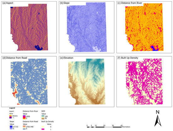
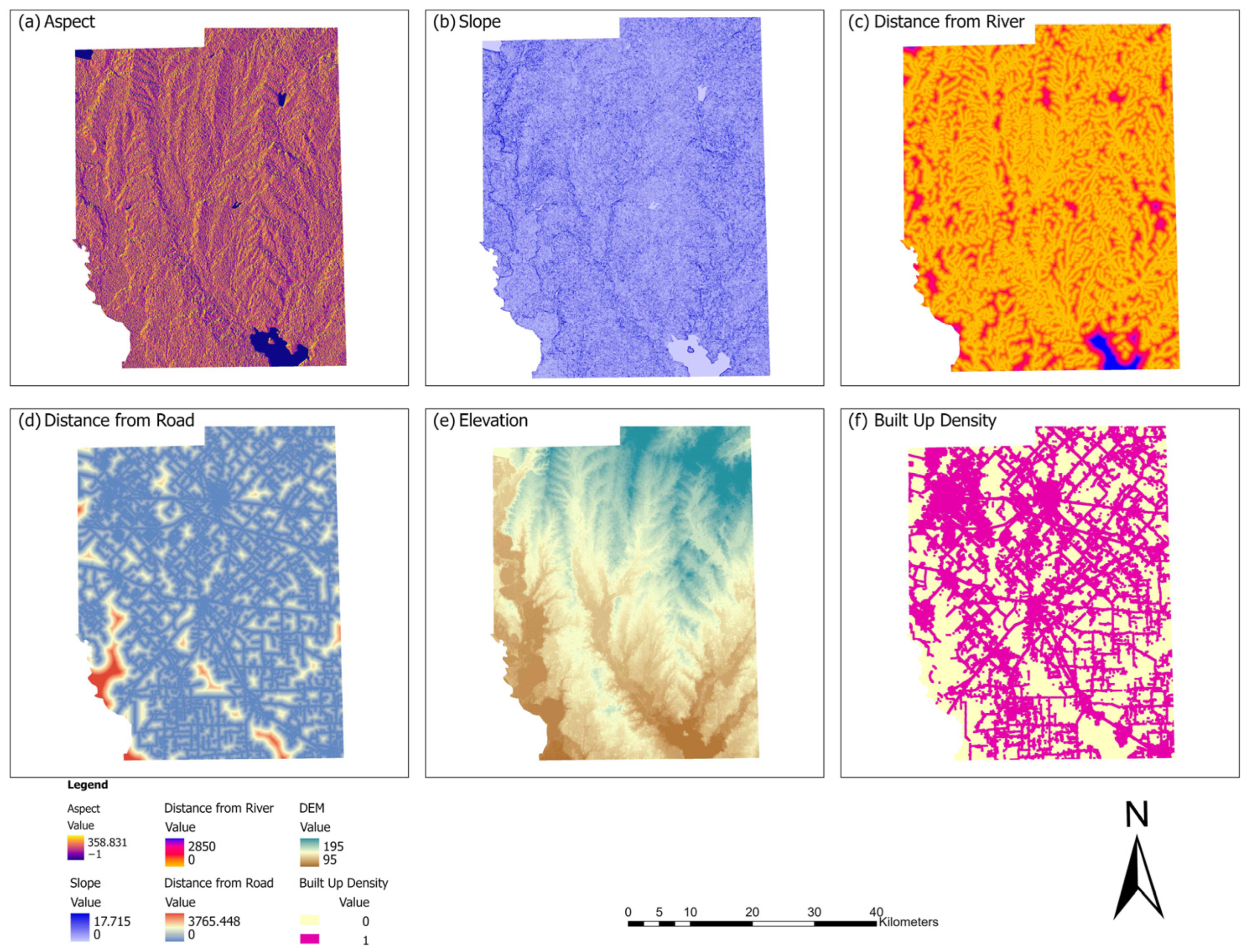
Spatially, six variables representing elevation (DEM), slope, aspect, distance to roads, distance to rivers, and built-up density (Figure 3) were used based on Pearson’s correlation coefficient [46,47] to represent the major physical and accessibility factors of land-use transitions in Kaufman County. Topographic parameters represent terrain suitability and environmental limitations, while distance and density parameters represent accessibility and urban development pressure factors. Each dataset was resampled to 30 m and normalized to a range of 0–1 to facilitate stable and fast learning for the ANN model [7]. The spatial coverage of each layer was cropped and fine-tuned to ensure all layers had the same spatial extent and resolution, to avoid scale differences in the analysis. The formatted data were loaded into the MOLUSCE plugin within QGIS version 3.42.3-Münster and used by the CA–ANN model to generate transition-potential surfaces [48] and simulate future spatiotemporal LULC patterns in Kaufman County, Texas.

Figure 3. Spatial explanatory variables used in this study.

2.4. LULC Classification Scheme

The original land-use and land-cover data were obtained from the NLCD, which has a detailed hierarchical classification system. For this study, the NLCD categories were reclassified into the six generalized classes (Table 2) for modeling and interpretation in the CA–ANN framework [18]. The six classes adopted for this study are based on regional land characteristics and previous LULC studies. The six final classes are: Built-up area, Forest, Open area, Cropland, Water, and Wetlands. The built-up area represents all impervious surfaces and man-made structures (e.g., residential, commercial, industrial, roads), the forest represents all tree-covered and dense vegetated land [49], and the open area represents sparsely vegetated land (e.g., grassland, rock, sand). The cropland [50] represents all cultivated and agricultural land, and the water represents all rivers, ponds, lakes, and reservoirs. Wetlands represent waterlogged areas, and marshes or swamps [51].

Table 2. Description of land-use and land-cover (LULC) classes.

	Class	Description
1	Built-up area	Areas covered by man-made infrastructure, including residential, commercial, and industrial zones, as well as roads and impervious surfaces.
2	Forest	Densely vegetated regions comprising trees and forested land, representing natural or semi-natural vegetation cover.
3	Open area	Land with sparse vegetation such as grasslands, shrublands, parks, and barren surfaces, including rocks and sand.
4	Cropland	Cultivated agricultural areas characterized by visible crop patterns or farming activities.
5	Water	Includes all forms of surface water such as rivers, lakes, ponds, and reservoirs.
6	Wetlands	Ecologically sensitive zones with a mix of water and vegetation, including marshes and swamps, that support rich biodiversity.

The aggregation of the NLCD subclasses to six general categories was performed to minimize the thematic fragmentation and imbalance in the sparsely distributed NLCD classes. Some of the NLCD subclasses have limited spatial extent in the study area, Kaufman County. These subclasses also have low transition frequency, which could cause instabilities during the ANN training process. The barren land NLCD subclass (NLCD 31) had a limited extent and was thus aggregated to the Green/Open area class. Although the individual NLCD subclasses may have localized variations in the transitions, the purpose of this study was to investigate the dominant land transition dynamics at the county level. Therefore, the results should be interpreted at the aggregated class level. All the explanatory variables were normalized to the range 0 to 1 before the modeling to ensure numerical stability during the ANN training process.

2.5. Transition Potential Modeling and Spatiotemporal Change Detection

The MOLUSCE plugin workflow involves importing datasets, correlation analysis, ANN training, and scenario simulation using CA model [8]. A change map was generated by overlaying the classified LULC layers from the two consecutive years. The change map shows the spatial distribution of expansion and reduction in the LULC classes. This indicates the direction of spatiotemporal change in the LULC, such as urban growth, vegetation loss, and agricultural transformation. Cross-tabulation analysis was used to compare LULC between the two periods and generated the transition matrix from observed pixel changes, indicating the proportion of the different LULC classes that changed. The ANN component was then trained to learn the nonlinear relationships between historical LULC transitions and spatial driving factors, producing transition potential maps that identify the spatial likelihood of change. While the transition matrix controls the quantity of change, the ANN-derived transition potential determines the spatial allocation of future LULC dynamics within the CA framework. Overall, the transition matrix and the classified change layer were used as inputs in the CA–ANN modeling to simulate and predict the future LULC dynamics in Kaufman County, Texas.

We used the Annual Rate of Change (ARC) [2,11,24] to figure out how fast and how big the changes in land use and land cover were for each class over the course of the study. This indicator shows the percentage change from one year to the next between two time periods. This makes it possible to compare growth and decline trends across categories. The ARC was computed using the following equation:

$$\mathrm{ARC}(\mathrm{\%})={\displaystyle \frac{F_y-I_y}{I_y\times t}}\times 100$$

(1)

where F_y and I_y represent the final and initial area (km²) of a given LULC category, respectively, and t is the time interval (years) between the two periods.

This method makes it possible to see how quickly each LULC class grew or shrank, showing how the landscape changed in Kaufman County over time, both in the past and in simulations.

2.6. CA–ANN Model Configuration

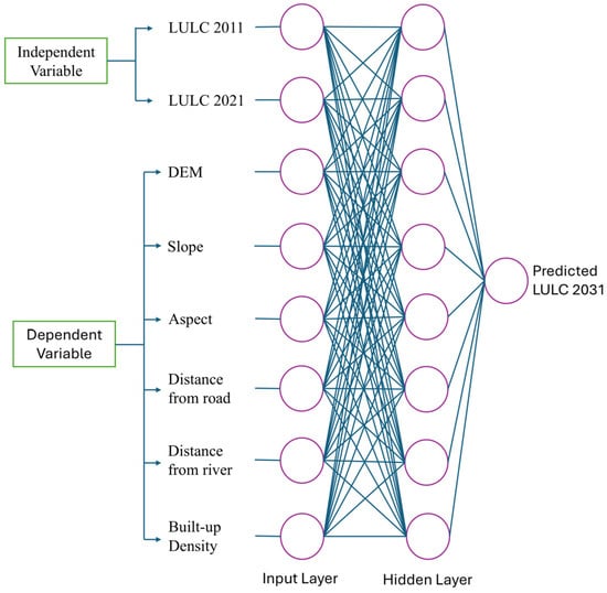
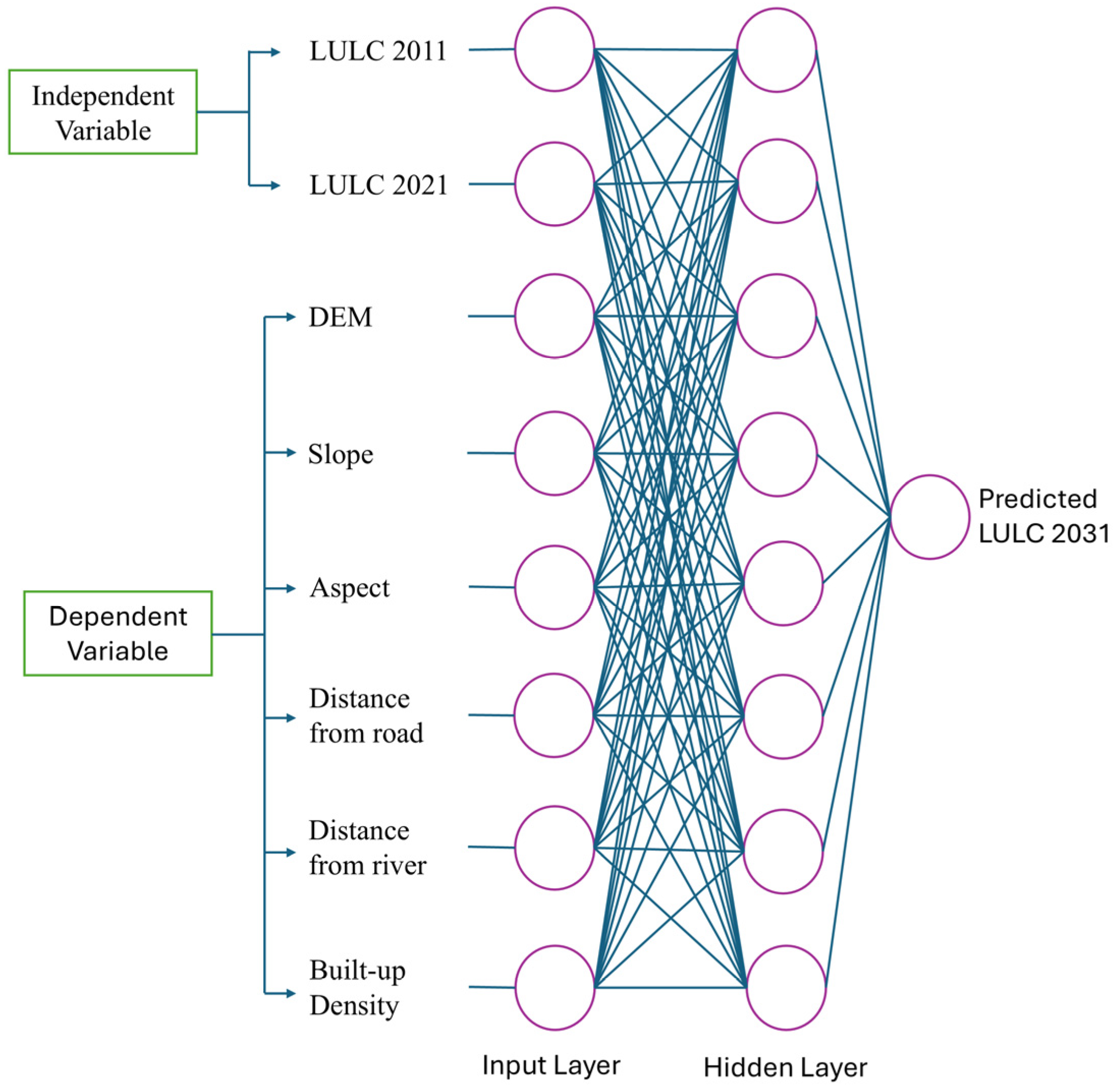
The Cellular Automata–Artificial Neural Network (CA–ANN) model [7] was prepared using the MOLUSCE plugin of QGIS. The CA–ANN model combines the strengths of both the ANN and CA. The ANN model (Figure 4) has powerful predictive capabilities of quantitative relationships between driving factors, while the CA model spatially transforms the LULC changes. The CA–ANN model, therefore, captures both quantitative and spatial dynamics of LULC. The ANN employed a multilayer perceptron architecture trained using stratified sampling [52,53] with 15,000 samples to ensure balanced representation across classes. The training samples were automatically generated in MOLUSCE by comparing the initial and final LULC maps (2001–2011), where sample pixels were selected from observed transition classes using stratified sampling to ensure that both stable and changing LULC categories were proportionally represented. The key parameters included a learning rate of 0.001, momentum of 0.05, maximum iterations of 1000, and 12 hidden neurons (units) within single hidden layers, with a 1-pixel neighborhood (3×3 pixel) defining spatial influence [6,10,32,54]. The transition potential maps generated from the ANN were then integrated into the CA framework to simulate spatial transitions based on neighborhood rules and transition probabilities. This allowed land-use transitions to propagate algorithmically through iterative CA steps, where the 3×3 neighborhood re-evaluates spatial contagion at each iteration, ensuring gradual expansion from adjacent cells rather than a fixed-window constraint. After validation, the calibrated CA–ANN model was used to simulate future LULC projection using the transition potentials and spatial driving factors in Kaufman County, Texas.

Figure 4. Architecture of the Artificial Neural Network (ANN) integrated within the CA–ANN model, where circles represent neurons (nodes) and connecting lines indicate weighted connections between layers.

2.7. Model Validation and Accuracy Assessment

Comparison of the simulated LULC map for the year 2021 with the observed NLCD 2021 data was carried out to determine the accuracy of the model during the historical validation stage. The accuracy of the model was determined using several statistical parameters, such as overall accuracy, Kappa (overall), Kappa (histogram), and Kappa (location). Overall accuracy is the ratio of the number of correctly classified pixels in the simulated and observed maps. Kappa (overall) is a parameter that shows the agreement in the simulated and observed maps, excluding the chance occurrence. Kappa (histogram) is a parameter that shows the similarity in the quantities of the classes in the simulated and observed maps. It shows the accuracy in the total area covered by each class in the land-use maps. Kappa (location) shows the accuracy in the distribution of the classes in the land-use maps. The accuracy results showed that the model performance was satisfactory, as the overall accuracy was 90.9%, Kappa (overall) was 0.84, Kappa (histogram) was 0.99, and Kappa (location) was 0.85 [55].

After the model performance was validated to be within acceptable limits, the trained CA–ANN model was used to produce transition potential maps using spatial driving factors that represented the conditions in the year 2021. Transition matrices based on historical LULC changes between 2011 and 2021 were used to determine the amount of land-use conversions, while transition potential maps were used to determine the spatial distribution of the conversions in the Cellular Automata simulation. Following this historical validation, conditional future LULC maps were produced for the years 2031, 2041, and 2051 using the CA allocation process, where one iteration in the simulation process represented a period of 10 years. Therefore, one, two, and three iterations in the CA simulation process were used to produce the LULC maps for the years 2031, 2041, and 2051, respectively. It is assumed that the relationship between the driving factors and land-use conversions that were evident in the historical period will still be evident in the projection period.

3. Results and Discussion

3.1. Historical LULC Dynamics

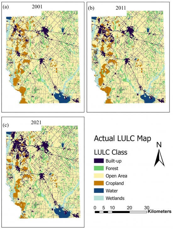
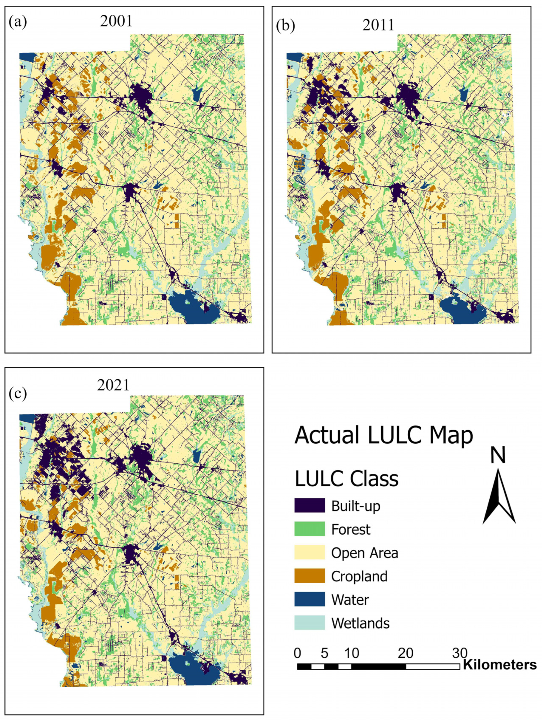
The overall area and ARC for each class are shown in Table 3. Built-up areas expanded from 180.44 km² (8.59%) in 2001 to 258.70 km² (12.32%) in 2021, recording the highest growth rate (ARC = 2.17%). In contrast, open area and cropland declined throughout the study period. Forest cover increased by approximately 8 km² per decade, while wetlands showed a negligible reduction. Water showed a decrease during 2001–2011 but gained in the second decade, likely reflecting enhanced surface-water storage and reservoir development. Table 3 shows the decadal change in each LULC class. Built-up areas increased by 38.04 km² (17.41%) from 2001–2011 and 40.22 km² (15.55%) from 2011–2021, with the highest transformation. Natural and agricultural land continued to decline, while forest and water slightly increased. Wetlands exhibited minimal net area change over the study period. Spatial distribution of historical LULC for 2001, 2011, and 2021 is shown in Figure 5.

Table 3. Area statistics, Area change with percentage variation, and annual rate of change (ARC) of LULC categories in Kaufman County (2001–2021).

LULC Type	2001		2011		2021		2001–2011		2011–2021		ARC%
	km2	%	km2	%	km2	%	km2	%	km2	%
Built-up	180.44	8.59	218.48	10.40	258.70	12.32	38	17.41	40.22	15.55	2.17
Forest	205.80	9.80	213.93	10.19	222.12	10.58	8.13	3.8	8.19	3.69	0.40
Open Area	1402.64	66.79	1372.53	65.36	1334.46	63.55	−30.1	−2.19	−38.1	−2.85	−0.24
Cropland	136.07	6.48	124.77	5.94	105.35	5.02	−11.3	−9.06	−19.4	−18.4	−1.13
Water	62.30	2.97	57.59	2.74	68.10	3.24	−4.71	−8.18	10.51	15.43	0.47
Wetlands	112.71	5.37	112.64	5.36	111.23	5.30	−0.07	−0.06	−1.41	−1.27	−0.07

Figure 5. LULC maps of Kaufman County for (a) 2001, (b) 2011, and (c) 2021.

Spatial and temporal distribution of LULC in Kaufman County in 2001, 2011, and 2021 reveals a pattern of long-term land transformation, where there has been rapid growth in built-up areas. From the temporal distribution of LULC in Kaufman County in 2001, 2011, and 2021, it is evident that the area of built-up is consistently increasing, especially along the transportation corridors. The spatial distribution of built-up area growth along the transportation corridors implies that accessibility and availability of infrastructural facilities are the major driving forces behind land transformation in Kaufman County. The fact that the area of cropland and open area is consistently declining implies that there has been a progressive transformation in land use in Kaufman County, where land is being converted to urban and infrastructural uses. This implies that there has been a structural transformation in land use in Kaufman County, where the focus has shifted from rural land use to urban land use. Forest and wetland areas have remained unchanged, while the area covered by water has increased.

The continued expansion of built-up areas in both decades validates the idea that urban growth is not a temporary phenomenon but is structurally embedded in the county’s growth pattern. The continued decline in cropland reflects a decrease in provisioning ecosystem services such as agricultural production potential. The conversion of cropland and open land into impervious surfaces may also reflect a decline in the infiltration capacity of the land, potentially leading to an increase in runoff and changes in hydrological processes. Although there is a moderate increase in forest cover, this should be considered in an ecological context. Forest expansion can reflect an increase in regulating ecosystem services such as carbon sequestration, microclimate moderation, erosion protection, and habitat provision. However, if this expansion is in fragmented patches rather than continuous expanses, this may not be effective in promoting ecological connectivity and biodiversity provision. The fluctuation and subsequent increase in water bodies during the second decade may reflect an improvement in regulating ecosystem services such as flood protection, surface water supply, and water supply reliability. Nevertheless, increasing urbanization may counteract some hydrological benefits by expanding impervious surfaces and accelerating runoff generation.

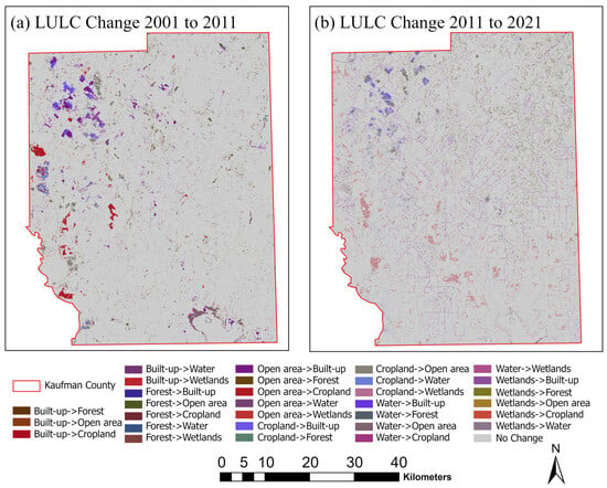
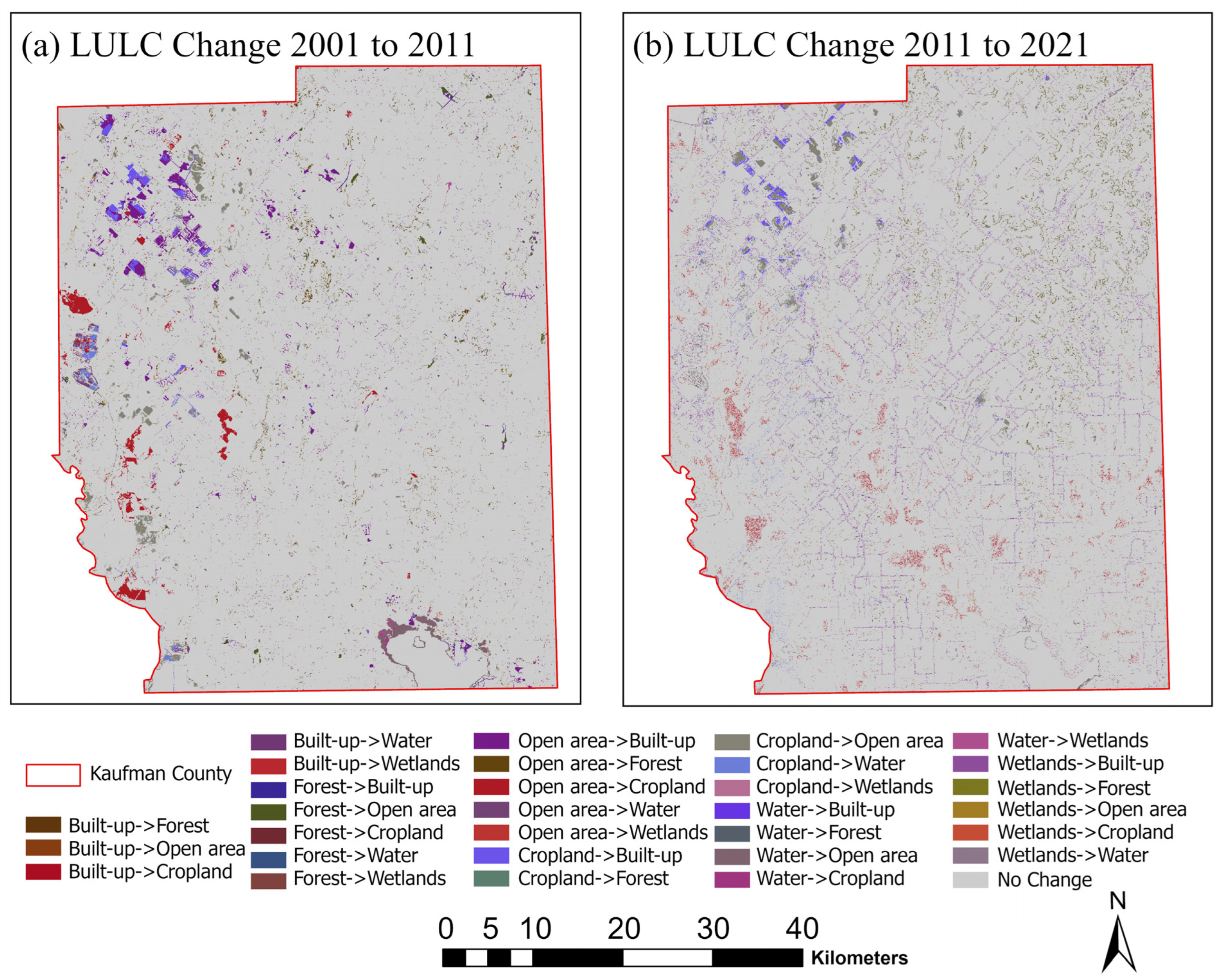
In general, these results reflect the overall conversion trend towards increasing urban intensification and the gradual loss of agricultural and open landscapes, consistent with regional urbanization patterns in the fast-growing Texas counties. The dominant transition from open and cropland to built-up land suggests that urban expansion is the primary mechanism driving landscape restructuring in Kaufman County. This directional pattern indicates a progressive shift toward urban land dominance, which may have long-term implications for land sustainability, ecosystem service provision, and spatial planning strategies. The distribution of these transitions across the county can be seen in the LULC change maps (Figure 6), showing the gain and loss areas for each LULC class. The spatial gain–loss patterns further confirm that built-up expansion largely corresponds with the spatial contraction of open and agricultural lands, reinforcing the interpretation that urbanization is the central force shaping recent landscape dynamics.

Figure 6. Spatial LULC change map for (a) 2001–2011, and (b) 2011–2021.

Overall, globally, rapid urbanization driven by population growth, economic development, and infrastructure expansion continues to transform natural landscapes [56]. A similar pattern is observed in Kaufman County, Texas, recently identified as the fastest-growing county in the state and the second fastest in the United States [39]. This remarkable demographic growth has also accelerated suburban sprawl, reflected in the historical and simulated LULC changes. The built-up area has increased rapidly along western and central corridors within the Dallas–Fort Worth metropolitan region, especially near Forney, Terrell, and Kaufman City. The transformation displaced cropland and open areas, creating a typical metropolitan-fringe pattern consistent with metropolitan-fringe development patterns commonly associated with population growth and infrastructure expansion [57]. Accessibility along major transportation corridors (e.g., U.S. 175, SH-34, and I-20) strongly constrains spatial growth, but environmental conditions such as topography and flood exposure may also influence development trends at the regional scale.

3.2. Transition Analysis

The transition matrix provides quantitative information about the likelihood of a given LULC class converting into another class for given time intervals. It expresses the percentage of pixels that changed from one category to another between two time periods. The rows of the matrix represent the initial LULC classes, while the columns represent the same classes in the final year. The values along the main class-to-class correspondence indicate the proportion of land that remained in the same category between the compared years, reflecting class stability. The off-class values represent transitions from one land-cover category to another during the specified interval. These matrices help to identify the dominant path of landscape change and how human activities, planning policies, and environmental constraints shape the spatial evolution in Kaufman County. In this study, transition matrices were first derived from observed historical LULC maps (2001–2011 and 2011–2021). These historical transition matrices were then integrated with ANN-derived transition potential maps within the CA framework to simulate future LULC patterns for 2031, 2041, and 2051. This modeling workflow follows the standard CA–ANN implementation within the MOLUSCE framework, as applied in previous studies by Abbas et al. [58].

For the 2001–2011 time period (Table 4), the built-up and wetlands categories showed the highest stability with probabilities 0.9919 and 0.9810, respectively, while the cropland showed the lowest transition potential (probability 0.8021 to remain in the same category), with the highest transition probability to built-up of 0.0563. Open areas showed intermediate stability (0.9537) and contributed roughly 2.16% to built-up and 1.08% to cropland, reflecting a phase of transition of open peri-urban areas around developing municipalities. For 2011–2021 (Table 4), the built-up category was the most stable (0.9931), followed by forest (0.9669) and water (0.9120). The Cropland category was the most dynamic, with 6.55% to built-up and 14.47% to open. This indicates a sustained land-use transformation reflecting the expanding influence of the Dallas–Fort Worth metropolitan area.

Table 4. Multi-Decadal LULC Transition Matrix for the Period 2001–2051.

From Class	To Class	2001–2011	2011–2021	2021–2031	2031–2041	2041–2051
Built-up	Built-up	0.9919	0.9931	0.9941	0.9871	0.9848
Built-up	Forest	0.0005	0.0002	0.0002	0.0003	0.0004
Built-up	Open Area	0.0074	0.0061	0.0052	0.0116	0.0132
Built-up	Cropland	0.0001	0.0000	0.0000	0.0001	0.0002
Built-up	Water	0.0002	0.0005	0.0005	0.0004	0.0005
Built-up	Wetlands	0.0000	0.0000	0.0000	0.0004	0.0008
Forest	Built-up	0.0058	0.0049	0.0041	0.0039	0.0037
Forest	Forest	0.9612	0.9669	0.9687	0.9565	0.9463
Forest	Open Area	0.0316	0.0251	0.0242	0.0353	0.0447
Forest	Cropland	0.0000	0.0001	0.0001	0.0002	0.0002
Forest	Water	0.0010	0.0025	0.0024	0.0031	0.0037
Forest	Wetlands	0.0004	0.0005	0.0005	0.0011	0.0015
Open Area	Built-up	0.0216	0.0235	0.0243	0.0269	0.0289
Open Area	Forest	0.0108	0.0109	0.0112	0.0137	0.0164
Open Area	Open Area	0.9537	0.9523	0.9508	0.9419	0.9306
Open Area	Cropland	0.0108	0.0048	0.0049	0.0081	0.0101
Open Area	Water	0.0026	0.0080	0.0083	0.0087	0.0131
Open Area	Wetlands	0.0005	0.0006	0.0006	0.0008	0.0010
Cropland	Built-up	0.0563	0.0655	0.0774	0.0710	0.0243
Cropland	Forest	0.0001	0.0003	0.0001	0.0003	0.0007
Cropland	Open Area	0.1199	0.1447	0.0886	0.0775	0.0838
Cropland	Cropland	0.8021	0.7721	0.8134	0.7992	0.8161
Cropland	Water	0.0208	0.0170	0.0201	0.0512	0.0739
Cropland	Wetlands	0.0008	0.0003	0.0004	0.0007	0.0012
Water	Built-up	0.0023	0.0016	0.0004	0.0012	0.0024
Water	Forest	0.0116	0.0025	0.0011	0.0037	0.0052
Water	Open Area	0.1518	0.0338	0.0284	0.0274	0.0823
Water	Cropland	0.0079	0.0410	0.0347	0.0651	0.0779
Water	Water	0.8078	0.9120	0.9277	0.8955	0.8242
Water	Wetlands	0.0186	0.0091	0.0077	0.0070	0.0080
Wetlands	Built-up	0.0014	0.0016	0.0019	0.0040	0.0048
Wetlands	Forest	0.0019	0.0014	0.0021	0.0029	0.0037
Wetlands	Open Area	0.0108	0.0061	0.0092	0.0094	0.0109
Wetlands	Cropland	0.0002	0.0006	0.0005	0.0008	0.0015
Wetlands	Water	0.0047	0.0159	0.0159	0.0159	0.0173
Wetlands	Wetlands	0.9810	0.9745	0.9703	0.9669	0.9618

For the three projected decades, the transition matrices for 2031, 2041, and 2051 (Table 4) show a gradual intensification of the urban dominance. In 2031, the built-up category is still the most stable (0.9941), while cropland shows increased conversion to built-up of 7.74% and open areas of 8.86%. In 2051, the stability of the built-up category decreases slightly to 0.9848 while cropland further increases the conversion to built-up with 0.0243 and water with 0.0739. Open areas contributed moderately to the built-up conversion of 0.0289. Therefore, the 0.4043 persistence indicates a small transfer of open areas to built-up areas in the following decades.

Overall, the transition matrices show that the built-up category is highly persistent, while cropland and open are the major contributors to urban conversion. The forest, water, and wetland categories show high stability and may be linked to their spatial distribution in areas prone to flooding [59], conservation areas, or low-development areas. The small but persistent loss of cropland indicates high pressure on land use, likely related to rapid population growth and the sprawl of urban fragments. These quantitative transition relationships form the basis for the CA–ANN-based simulation of future LULC changes, and each category is then simulated to spatially reflect the transition probabilities from its historical transformations under the existing development pattern in Kaufman County.

3.3. Driving Factor Screening and Multicollinearity Analysis

Pearson’s correlation analysis (Table 5) was conducted to examine linear relationships among the selected driving variables and identify potential multicollinearity before CA–ANN model calibration. Variables exhibiting strong intercorrelation were evaluated for redundancy to ensure model stability and reduce overlapping explanatory effects. The initially selected variables were DEM, slope, distance from river, distance from road, distance from built-up areas, built-up density, and aspect. The Pearson correlation values vary between −1 and +1, and values closer to −1 or +1 indicate a stronger relationship. Values close to 0 show no or negligible correlation.

Table 5. Pearson correlation matrix of explanatory variables.

	DEM	Distance from Road	Slope	Distance from River	Built-Up Density	Aspect
DEM	--
Distance from Road	−0.3295	--
Slope	0.0217	−0.0739	--
Distance from River	−0.1495	0.1605	−0.1305	--
Built-up Density	0.1976	−0.5482	0.0198	−0.0134	--
Aspect	0.0436	−0.0617	0.1065	−0.1249	0.0303	--

The correlation matrix showed a moderate negative relationship for the distance from the road and DEM (r = −0.3295), meaning that higher elevation areas tend to be closer to the road, while lower-lying areas are generally farther away. The moderate negative correlation between Distance from road and Built-up density (r = −0.5482) shows that the urban growth is often clustered along the roads. A strong positive correlation coefficient value of r = 0.813 was found for the variables “distance from built-up” and “distance from road.” This suggests a potential redundancy for these two accessibility-related variables. To minimize this multicollinearity issue, “distance from built-up” was not included in the final CA–ANN model configuration; however, “distance from road” was included as a predictor for infrastructure accessibility. Other predictor variables had weak to moderate linear correlations, which suggests a lack of redundancy for these variables. The nonlinear effects of the selected drivers for LULC changes were modeled within the ANN component of the CA–ANN model. Pearson’s correlation analysis was mainly employed for the exploration of linear relationships, as well as for the detection of possible multicollinearity between the explanatory variables, rather than for the assessment of the relative importance of the drivers in the CA–ANN model. The ANN part of the model is able to detect the nonlinear relationships between the drivers of the land transitions during the training of the model, which cannot be achieved by the linear correlation coefficients. Hence, the correlation matrix was employed for the improvement of the stability of the model, while the relative importance of the drivers is implicitly incorporated during the calibration of the CA–ANN model.

3.4. Calibration and Validation Performance of the CA–ANN Model

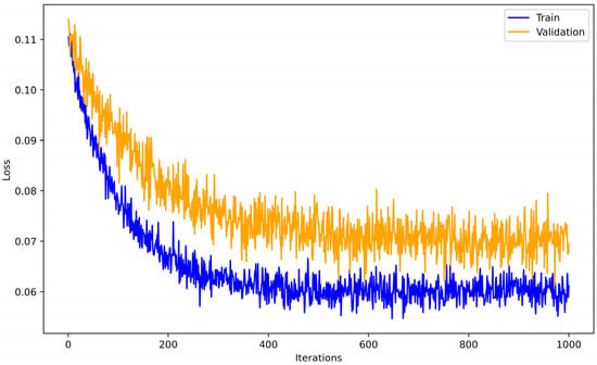
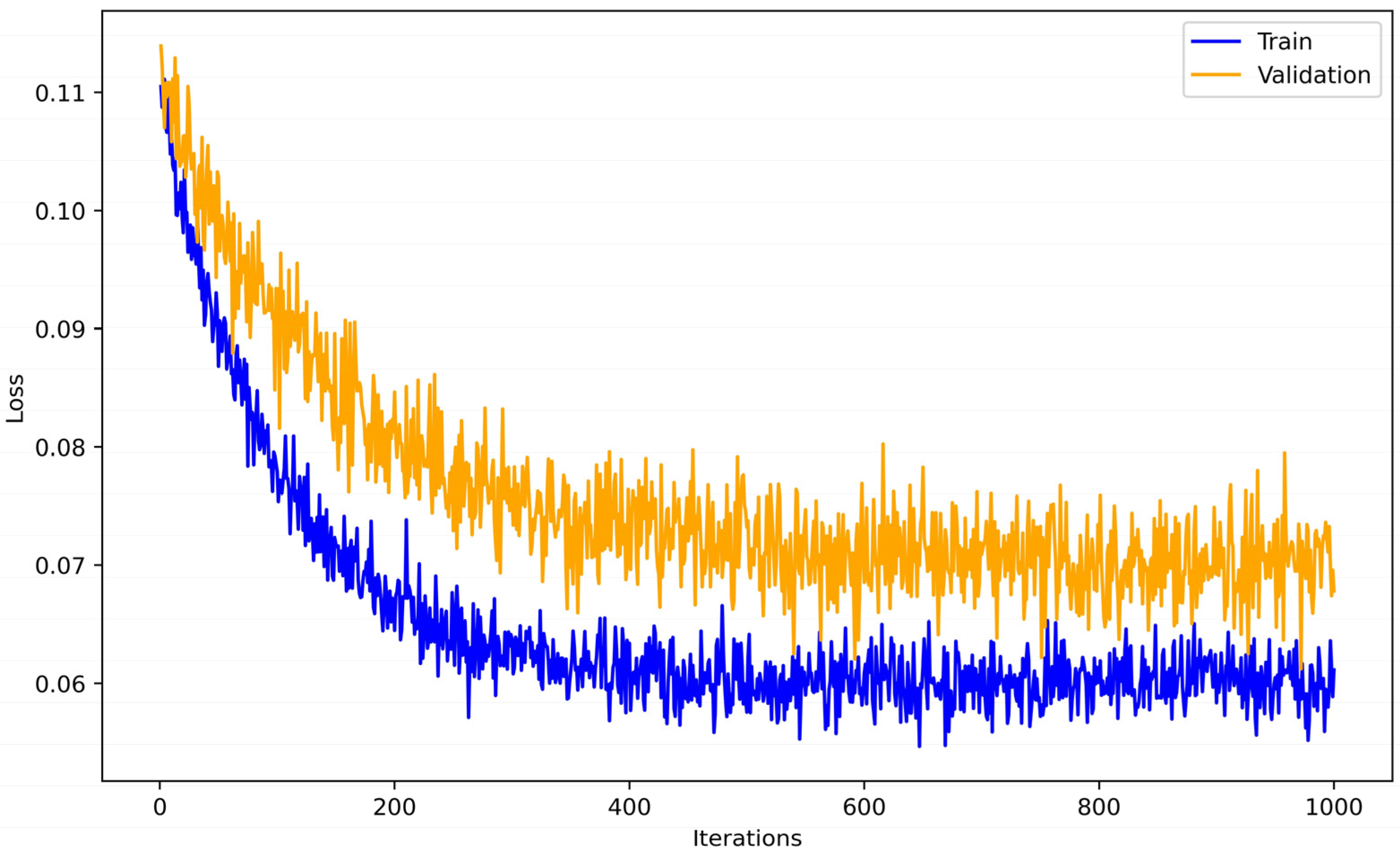
The neural network learning curve [2,24,60,61] in Figure 7 shows a clear and constant decrease in training and validation errors before stabilizing around 800 iterations. This indicates the convergence of the model and good learning. Results confirmed that the CA–ANN model was well-calibrated and captured the spatial complexity of land-use changes, and the high accuracy supports its application for long-term LULC prediction in Kaufman County.

Figure 7. Neural Network Learning curve during calibration period.

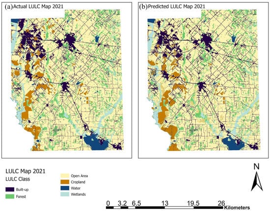
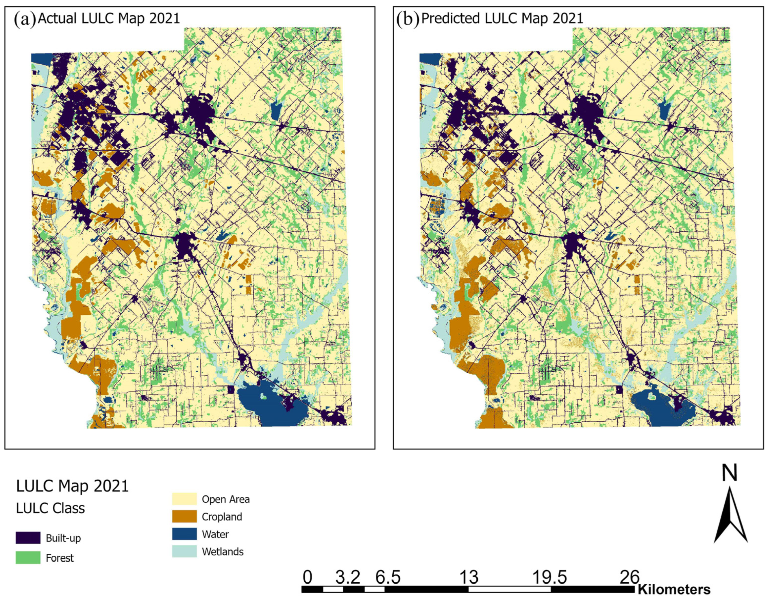
Model validation was performed using spatial drivers of 2011 and setting iteration as 1 while keeping 2001 LULC as initial and 2011 LULC as final for initial setup and checking the accuracy of the CA–ANN simulation by comparing the actual LULC and simulated 2021 LULC. These results (Table 6) show high consistency and confirm the model’s reliability in reproducing the observed 2021 LULC (Figure 8). The total area under each LULC category showed only a small deviation from the total area, with built-up, forest, and open areas showing the highest consistency between simulated and actual values. The model had Kappa (overall) = 0.84, Kappa (histogram) = 0.99, Kappa (location) = 0.85, and an overall percent correctness of 90.9%. This indicated a high spatial and categorical agreement between the predicted and actual LULC, confirming the model was well-calibrated and indicating strong agreement between simulated and observed LULC during the historical validation period. The high Kappa (location) value indicates that the model effectively reproduced the spatial allocation of land-cover classes, while the high Kappa (histogram) value reflects strong agreement in class quantity distribution. The relatively small differences in total area among major classes suggest that transition potentials were appropriately captured during training. Together, these results indicate that the CA–ANN model reliably represented both spatial configuration and class proportions during the historical validation interval.

Table 6. Validation of the CA–ANN model showing strong agreement between actual and projected LULC for 2021.

LULC Type	Actual 2021		Projected 2021		Kappa Value			% of Correctness
	km2	%	km2	%	Overall	Histogram	Location
Built-up	258.70	12.32	256.55	12.22	0.84	0.99	0.85	90.9
Forest	222.12	10.58	222.23	10.58
Open Area	1334.46	63.55	1339.64	63.79
Cropland	105.35	5.02	116.16	5.53
Water	68.10	3.24	53.71	2.56
Wetlands	111.23	5.30	111.67	5.32

Figure 8. Comparison of actual and projected LULC maps for 2021: (a) Actual LULC derived from NLCD data, and (b) Projected LULC from the CA–ANN model.

Overall, the agreement between observed and simulated 2021 maps demonstrates that the model can reproduce observed spatial transition patterns based on the selected explanatory variables. The hybrid framework successfully captured the nonlinear urban pattern with 30 m NLCD data, but small inaccuracies with the cropland and water categories result from the static nature of the explanatory variables and the decadal nature of the data. Therefore, the CA–ANN model proved reliable for regional-scale simulation predictions, consistent with observed regional urban expansion trends.

3.5. Future LULC Projections and Spatial Change Analysis

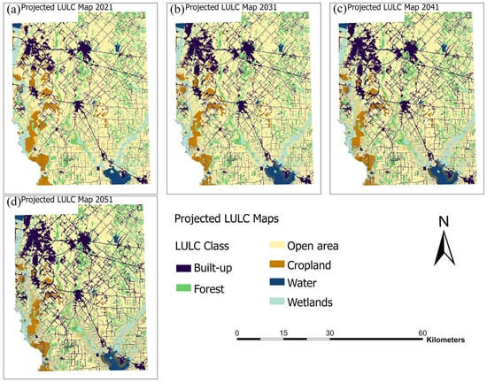
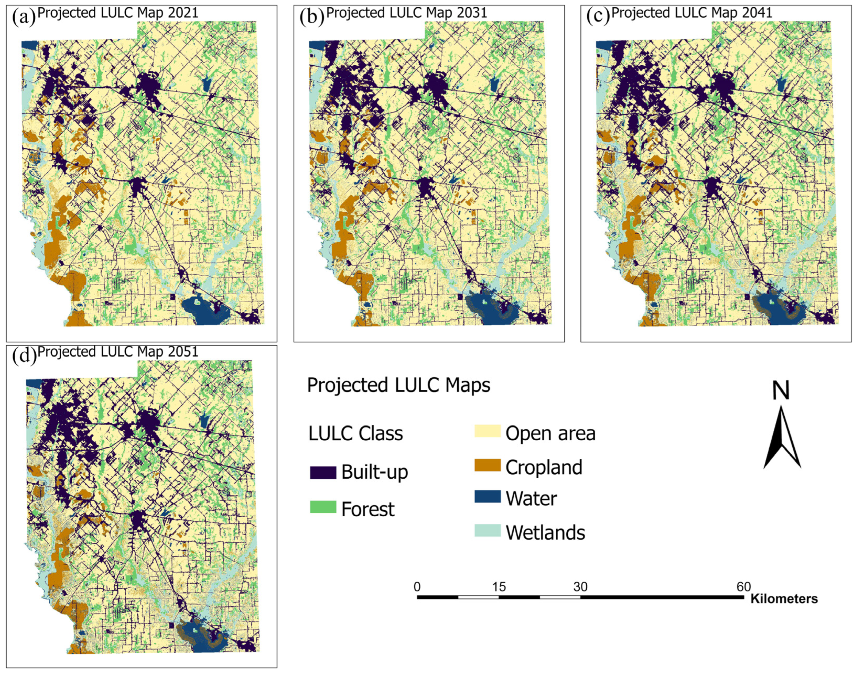
The calibrated CA–ANN model was used to simulate the LULC for the years 2031, 2041, and 2051 using the 2011–2021 transition probability and spatial factors as conditional simulations. The projected LULC category distribution is shown in Table 7, and projected LULC maps for the years 2031, 2041, and 2051 are shown in Figure 9.

Table 7. Baseline (2021) and Projected Land-Use/Land-Cover Changes for 2031, 2041, and 2051 with percentage change.

Class Category	2021 Baseline	2031 Projection			2041 Projection			2051 Projection
	2021 Area (km2)	2031 Area (km2)	2031 Change (km2)	2031% Change	2041 Area (km2)	2041 Change (km2)	2041% Change	2051 Area (km2)	2051 Change (km2)	2051% Change
Built-up	258.7	298.91	40.21	13.45	337.82	79.12	23.42	372.17	113.47	30.49
Forest	222.12	230.43	8.31	3.61	238.79	16.67	6.98	247.2	25.08	10.15
Open Area	1334.46	1287.79	−46.67	−3.62	1235.12	−99.34	−8.04	1180.7	−153.76	−13.02
Cropland	105.35	94.7	−10.65	−11.24	91.35	−14	−15.33	94.31	−11.04	−11.71
Water	68.1	78.74	10.64	13.52	89.11	21.01	23.58	99.27	31.17	31.4
Wetlands	111.23	109.38	−1.85	−1.69	107.77	−3.46	−3.21	106.31	−4.92	−4.63

Figure 9. Projected LULC maps generated using the CA–ANN model (a) 2021, (b) 2031, (c) 2041, and (d) 2051.

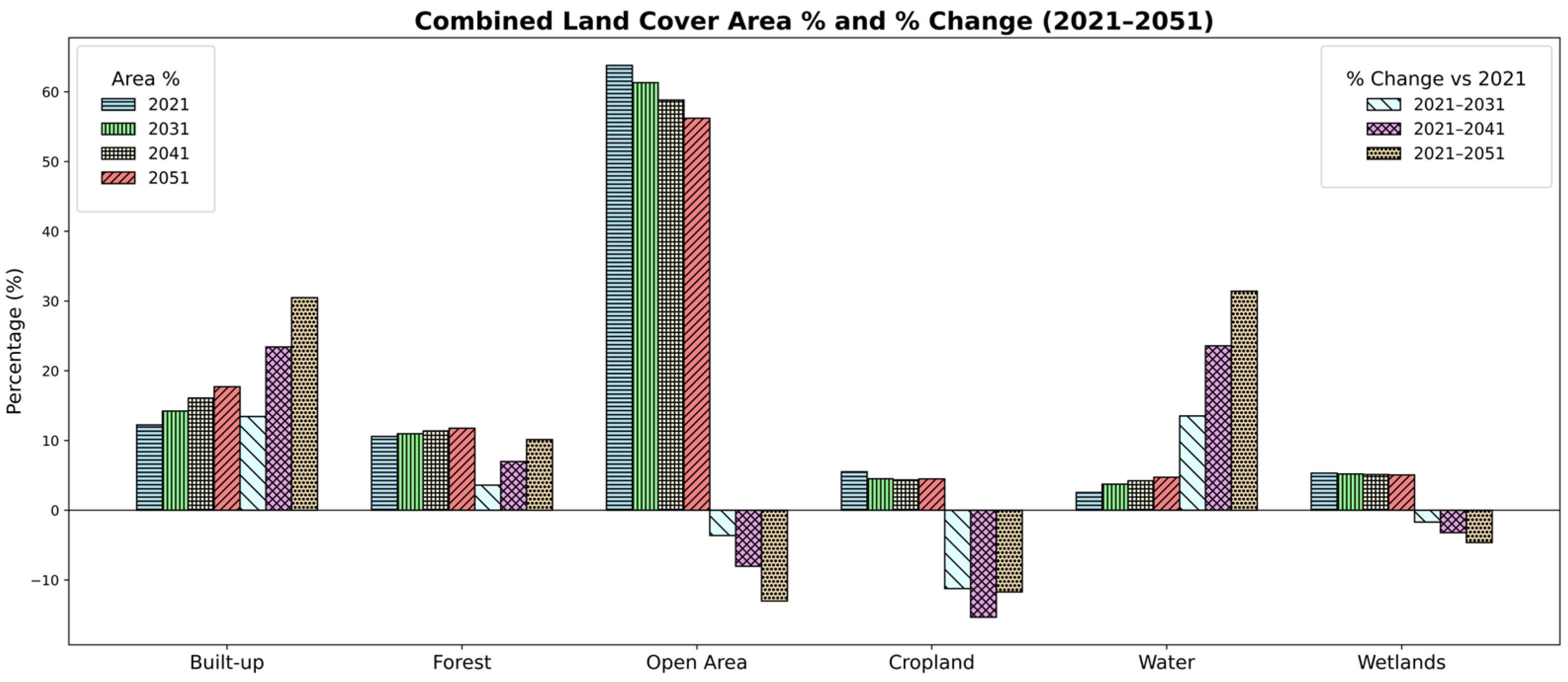
From 2021 to 2031, built-up area is predicted to increase from 258.70 km² to 298.91 km² (+13.45%) due to continued suburban sprawl (especially in western Kaufman County) driven by the nearby Dallas–Fort Worth metropolitan region. Forest area (+3.61%) and water (+13.52%) are predicted to increase, whereas open area (−3.62%), cropland (−11.24%), and wetlands (−1.69%) are predicted to decrease (Table 7). By 2041, the built-up class continues to increase to 337.82 km² (+23.42%) along U.S. Highway 175, State Highway 34, and Interstate 20. Cropland and open areas continue to decrease (−15.33% and −8.04%), while water (+23.58%) increases significantly (Table 7). By 2051, the built-up land will reach 372.17 km² (+30.49%), indicating sustained urbanization. Open areas (−13.02%) and cropland (−11.71%) continue to decrease, while forest (+10.15%) and water (+31.40%) increase moderately, and wetlands show a gradual decline of about 4.6% during the simulation period (Table 7).

The projected decline in cropland and open areas, together with sustained built-up expansion, suggests a continued shift from permeable and productive landscapes toward more impervious and development-dominated surfaces. This transition may influence multiple ecosystem functions, including reduced agricultural production capacity, altered hydrological response through increased runoff potential, and fragmentation of semi-natural habitats. Although forest and water areas show moderate increases in total extent, the ecological benefits of these gains depend on spatial configuration and connectivity. If forest expansion occurs in isolated or edge-dominated patches, improvements in carbon sequestration, habitat quality, or biodiversity support may remain limited. Similarly, increases in water surface area may reflect hydrological redistribution rather than the enhancement of aquatic ecosystem services. Therefore, while aggregate area changes indicate directional trends, the spatial arrangement of land-cover transitions plays a critical role in determining their functional implications at the county scale.

This pattern of corridor-oriented suburbanization and conversion of agricultural land is consistent with studies of the urban fringe in rapidly growing metropolitan regions. For instance, such a study was performed by Kocur-Bera et al. in the urbanizing area of Poland, Surya et al. in Metropolitan Urban Area of South Sulawesi Province, Indonesia, and Sanchez et al. in urban development and state highway project corridors in Oregon [62,63,64], where transportation accessibility is a primary driver of urban expansion. Similar to these studies, the pattern of built-up expansion in Kaufman County is concentrated along major highway corridors and adjacent to existing urban clusters, suggesting an edge-driven pattern of expansion rather than dispersed growth. Regional CA–ANN studies in rapidly growing environments, such as the future LULC simulation study performed by Jain et al. for Delhi and Zhao et al. for Ya’an City area of China [8,65], also show similar results for cropland and open land as the primary source classes for urban expansion, where distance to road and proximity to development variables strongly influence transition probabilities. The results obtained in this study match the documented transition paths while offering a county-level evaluation in a US metropolitan fringe context. Unlike megacity studies, this work emphasizes the role of suburbanization dynamics in a lower-density environment.

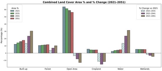
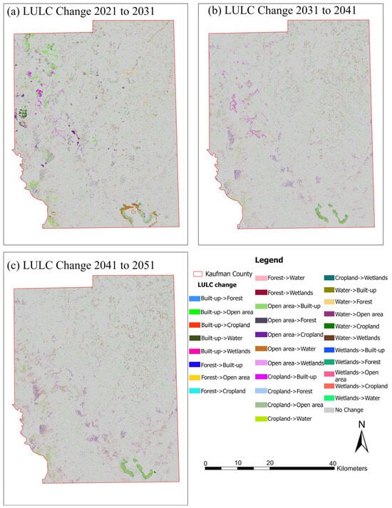
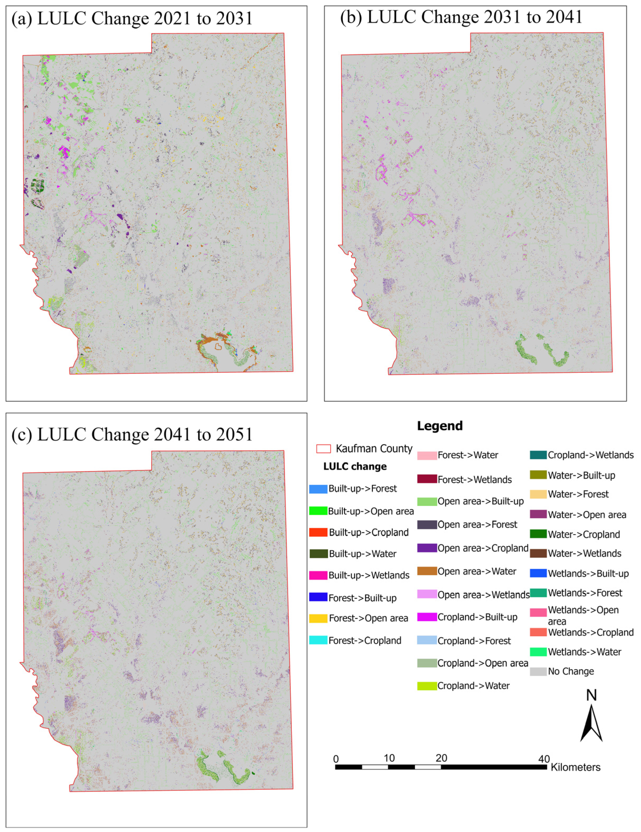
The comparative bar chart (Figure 10) shows the area proportion and percentage change for each LULC class for 2021, 2031, 2041, and 2051, clearly depicting the dominance of built-up growth and the steady loss of cropland and open areas. The simulated LULC maps and change-detection maps (Figure 11) further demonstrate that the most active urban expansion zones are also around Forney, Terrell, and central Kaufman County, extending mainly along major transportation corridors. Spatial change detection maps show that expansion of built-up areas is primarily concentrated along existing transportation corridors and near existing urban clusters. This suggests an edge expansion pattern for Kaufman County. The major transition pattern for all projection intervals is cropland-to-built-up changes, followed by open area-to-built-up changes. These changes show a contiguous pattern, implying accessibility and proximity to existing development as the primary driver for land conversion. Large portions of eastern and southern Kaufman County exhibit relative stability, with limited transitions outside major infrastructure corridors. Forest and water changes do not show a widespread pattern throughout Kaufman County but appear localized. This spatial pattern indicates that projected growth is structured and corridor-oriented rather than uniformly distributed.

Figure 10. Combined bar chart showing LULC area proportion and percentage change from 2021 to 2031, 2041, and 2051.

Figure 11. Change-detection maps for (a) 2021–2031, (b) 2031–2041, and (c) 2041–2051.

Overall, Future projections indicate that built-up land will increase by nearly 30% by 2051, mainly at the expense of cropland and open areas. Forest and water are projected to expand moderately according to the simulated land-cover transition trends. Wetlands show a gradual decline, reaching about 4–5% by 2051, with slight localized reductions observed in the projections. These transitions present larger tradeoffs between urban growth and ecological sustainability [66], where continuous expansion can intensify runoff [67], reduce agricultural productivity, and fragment vegetative cover [68]. Such outcomes are consistent with the current developed pattern driven by unprecedented population growth in Kaufman County, highlighting the need for growth management and environmental preservation. These results may contribute to informing policy and planning [69]. The county’s Comprehensive Plan supports corridor-based development, but the simulated spillover into growth zones suggests the need for stricter zoning, infrastructure controls, and conservation initiatives. Incorporating CA–ANN projections into regional planning can help identify urban hotspots, allocate land, and prioritize greenbelt preservation [70].

3.6. Policy Implications and Planning Relevance

The results obtained in the form of scenarios using the CA–ANN model provide useful information for the decision-maker to identify the areas where land-use transitions are likely to occur under scenario-based simulations. Even though the model does not include the projection of demographic changes, zoning regulations, conservation strategies, and floodplain constraints, the results obtained can provide useful insights to the decision-maker to identify the areas where land-use transitions are likely to occur. With the results obtained using the proposed CA–ANN model, the decision-maker can benefit in the following ways:

Strategic Spatial Screening: Areas identified with higher probabilities for the expansion of built-up land use can be identified and further analyzed for infrastructure capacity and services.

Agricultural Land Consideration: Zones showing increased likelihood of cropland-to-built transitions may warrant closer evaluation within local land preservation or growth management frameworks, depending on policy objectives.

Green Space and Ecological Planning Dialogue: Spatial patterns of simulated landscape change may help planners identify locations where maintaining ecological connectivity or open-space continuity could be strategically evaluated.

Integrated Planning Discussions: The outputs can serve as a complementary decision-support layer when combined with regulatory, environmental, and socio-economic datasets not included in the present model.

It is important to emphasize that these implications are conditional upon the modeled assumptions and historical transition relationships. The projections should therefore be interpreted as spatial likelihood scenarios rather than deterministic forecasts of future development.

3.7. Limitations of This Study

Although the CA–ANN model achieved strong agreement during validation, several limitations should be acknowledged. First, A formal uncertainty or sensitivity analysis was not conducted to quantify how variations in input drivers or model parameters may influence projected outcomes [57]. As a result, the robustness of long-term projections (2031–2051) to alternative driver configurations or parameter settings was not explicitly tested. Model validation was performed through forward simulation from 2011 to 2021 using independent temporal data; however, additional validation strategies such as back-casting across multiple historical intervals could further strengthen the assessment of temporal transferability and structural robustness. Second, the future simulations were generated using the 2021 spatial driver layers as fixed baseline conditions. This assumption implies continuation of observed spatial relationships and does not account for potential changes in infrastructure, climate conditions, or policy interventions [58]. Therefore, the projected maps should be interpreted as scenario-based simulations under constant driver assumptions rather than deterministic forecasts. Third, the 30 m NLCD data, although adequate for regional-scale applications, may ignore finer-scale urban infill changes and wetlands [71]. In addition, the original NLCD subclasses were aggregated into six broader land-cover classes to reduce class imbalance and improve model stability. This aggregation may mask finer distinctions within subclasses, and results should therefore be interpreted at the aggregated class level. Finally, this study applied a single CA–ANN framework. Although widely used in LULC modeling, a systematic comparison with alternative models (e.g., CA–Markov or CLUE-S) was not performed. Multi-model comparison could provide additional insight into model performance under different structural assumptions. Future research may incorporate structured sensitivity testing, dynamic socio-economic projections, stakeholder engagement, participatory scenario development, higher-resolution datasets, and comparative modeling approaches to further enhance robustness and practical applicability.

4. Conclusions

This study utilized a hybrid Cellular Automata–Artificial Neural Network model within the QGIS MOLUSCE platform to examine historical land-use and land-cover change dynamics in Kaufman County, Texas. The model reproduced observed transitions between 2001 and 2021 with strong validation performance (Kappa = 0.84; overall accuracy = 90.9%), indicating its capacity to simulate spatial transition patterns based on the selected explanatory drivers.

Under the assumption of continued historical transition trends, it is projected that built-up land-use classes show a considerable increase in Kaufman County by 2051, primarily at the expense of cropland and open land classes. Forest and water land-use classes show moderate expansion in this scenario, while wetland classes show minor changes. These projected patterns reflect the statistical relationships embedded in the CA–ANN framework and should be interpreted as scenario-based simulations rather than deterministic forecasts.

The simulated results indicate a potential increase in landscape imperviousness if the current transition trajectories continue. Although this model does not explicitly include demographic, zoning, conservation, or floodplain regulatory layers within the landscape change process, it does offer a level of spatial insight into where landscape change is more likely to occur.

The study demonstrates the applicability of CA–ANN modeling using accessible, open-source tools for examining nonlinear spatial dynamics of urbanization. However, future work could enhance robustness by incorporating additional drivers (e.g., socio-economic variables, climate indicators), conducting formal sensitivity and uncertainty analysis, and exploring alternative hybrid frameworks (e.g., CA–ANN–Markov or agent-based approaches). Such improvements would strengthen the interpretability and policy relevance of long-term scenario simulations.

References

- Gaur, S.; Singh, R. A Comprehensive Review on Land Use/Land Cover (LULC) Change Modeling for Urban Development: Current Status and Future Prospects. Sustainability 2023, 15, 903. [Google Scholar] [CrossRef] [Scilit]
- Mishra, O.; Khatiwada, N.; Joshi, D.; Gharti, S.; Khatri, B. Prediction of Land Use Land Cover Change Using a Coupled CA-ANN Modeling in Dhanusha District of Nepal. Res. Sq. 2024. [Google Scholar] [CrossRef] [Scilit]
- Amoah, M.K.M.; Gorsevski, P.V. Predicting Land Use Land Cover Changes and Impact on Urban Wetlands Using Cellular Automata and Artificial Neural Networks Approach, a Case Study in Greater Accra, Ghana. Sci. Afr. 2025, 28, e02767. [Google Scholar] [CrossRef] [Scilit]
- Dahal, D.; Bhattarai, N.; Silwal, A.; Shrestha, S.; Shrestha, B.; Poudel, B.; Kalra, A. A Review on Climate Change Impacts on Freshwater Systems and Ecosystem Resilience. Water 2025, 17, 3052. [Google Scholar] [CrossRef] [Scilit]
- Poudel, B.; Dahal, D.; Shrestha, S.; Sewa, R.; Kalra, A. Developing a Composite Drought Indicator Using PCA Integration of CHIRPS Rainfall, Temperature, and Vegetation Health Products for Agricultural Drought Monitoring in New Mexico. Atmosphere 2025, 16, 818. [Google Scholar] [CrossRef] [Scilit]
- Baghel, S.; Kothari, M.K.; Tripathi, M.P.; Singh, P.K.; Bhakar, S.R.; Dave, V.; Jain, S.K. Spatiotemporal LULC Change Detection and Future Prediction for the Mand Catchment Using MOLUSCE Tool. Environ. Earth Sci. 2024, 83, 66. [Google Scholar] [CrossRef] [Scilit]
- Gharaibeh, A.; Shaamala, A.; Obeidat, R.; Al-Kofahi, S. Improving Land-Use Change Modeling by Integrating ANN with Cellular Automata-Markov Chain Model. Heliyon 2020, 6, e05092. [Google Scholar] [CrossRef] [Scilit]
- Jain, M. Future Land Use and Land Cover Simulations with Cellular Automata-Based Artificial Neural Network: A Case Study over Delhi Megacity (India). Heliyon 2024, 10, e34662. [Google Scholar] [CrossRef] [Scilit] [PubMed]
- Kumari, S.; Roy, A. Simulation of Land Use and Land Cover Using the MOLUSCE Plugin Integrated with QGIS for the Western Himalayan Region of India. Int. Arch. Photogramm. Remote Sens. Spat. Inf. Sci. 2025, 48, 81–85. [Google Scholar] [CrossRef] [Scilit]
- Alshari, E.A.; Gawali, B.W. Modeling Land Use Change in Sana’a City of Yemen with MOLUSCE. J. Sens. 2022, 2022, 7419031. [Google Scholar] [CrossRef] [Scilit]
- Sabri, N.Q.; Khayyun, T.S. Spatiotemporal Prediction of Future LULC Changes, Northern and Northeastern Parts of Iraq with MOLUSCE. J. Ecohumanism 2024, 3, 2417–2433. [Google Scholar] [CrossRef] [Scilit]
- Tahir, Z.; Haseeb, M.; Mahmood, S.A.; Batool, S.; Abdullah-Al-Wadud, M.; Ullah, S.; Tariq, A. Predicting Land Use and Land Cover Changes for Sustainable Land Management Using CA-Markov Modelling and GIS Techniques. Sci. Rep. 2025, 15, 3271. [Google Scholar] [CrossRef] [Scilit]
- Wahdatyar, R.; Khokhar, M.F.; Ahmad, S.; Rahil, M.U.; Stanikzai, M.A.; Khan, J.A.; Kamran. Exploring the Dynamics and Future Projections of Land Use Land Cover Changes by Exploiting Geospatial Techniques; A Case Study of the Kabul River Basin. Heliyon 2024, 10, e39020. [Google Scholar] [CrossRef] [Scilit]
- Alkaraki, K.F.; Hazaymeh, K.; Al-Tarawneh, O.M.; Jawarneh, R.N. Deep Learning-Based Modeling of Land Use/Land Cover Changes Impact on Land Surface Temperature in Greater Amman Municipality, Jordan (1980–2030). GeoJournal 2024, 89, 170. [Google Scholar] [CrossRef] [Scilit]
- Megersa, W.; Deribew, K.T.; Abreha, G.; Liqa, T.; Moisa, M.B.; Hailu, S.; Worku, K. Stochastic Modeling of Urban Growth Using the CA-Markov Chain and Multi-Scenario Prospects in the Tropical Humid Region of Ethiopia: Mettu. Geocarto Int. 2023, 38, 2240285. [Google Scholar] [CrossRef] [Scilit]
- Khan, D.; Khan, N. Modelling Urban Future: Integrating CA-ANN Model for Comprehensive Understanding of Land Use, Land Cover Changes, and Temperature Dynamics in Lucknow City, India. Geol. Ecol. Landsc. 2025, 1–26. [Google Scholar] [CrossRef] [Scilit]
- Homer, C.; Dewitz, J.; Jin, S.; Xian, G.; Costello, C.; Danielson, P.; Gass, L.; Funk, M.; Wickham, J.; Stehman, S.; et al. Conterminous United States Land Cover Change Patterns 2001–2016 from the 2016 National Land Cover Database. ISPRS J. Photogramm. Remote Sens. 2020, 162, 184–199. [Google Scholar] [CrossRef] [Scilit] [PubMed]
- Yang, L.; Jin, S.; Danielson, P.; Homer, C.; Gass, L.; Bender, S.M.; Case, A.; Costello, C.; Dewitz, J.; Fry, J.; et al. A New Generation of the United States National Land Cover Database: Requirements, Research Priorities, Design, and Implementation Strategies. ISPRS J. Photogramm. Remote Sens. 2018, 146, 108–123. [Google Scholar] [CrossRef] [Scilit]
- Sohl, T.L.; Sayler, K.L.; Bouchard, M.A.; Reker, R.R.; Friesz, A.M.; Bennett, S.L.; Sleeter, B.M.; Sleeter, R.R.; Wilson, T.; Soulard, C.; et al. Spatially Explicit Modeling of 1992–2100 Land Cover and Forest Stand Age for the Conterminous United States. Ecol. Appl. 2014, 24, 1015–1036. [Google Scholar] [CrossRef] [Scilit]
- Oli, D.; Gyawali, B.; Neupane, B.; Oshikoya, S. Assessment of Land Use Land Cover Change and Its Impact on Variations of Land Surface Temperature in Atlanta, USA. Environ. Sustain. Indic. 2025, 26, 100712. [Google Scholar] [CrossRef] [Scilit]
- Guo, J.; Zhang, M.; Biłozor, A.; Salvati, L. Exploring the Patterns and Drivers of Urban Expansion in the Texas Triangle Megaregion. Land 2021, 10, 1244. [Google Scholar] [CrossRef] [Scilit]
- Zhao, C.; Weng, Q.; Hersperger, A.M. Characterizing the 3-D Urban Morphology Transformation to Understand Urban-Form Dynamics: A Case Study of Austin, Texas, USA. Landsc. Urban Plan. 2020, 203, 103881. [Google Scholar] [CrossRef] [Scilit]
- Saharkar, U.R.; Shahapure, S.S. Identification of Land Use Land Cover (LULC) Changes Using Geo-Spatial Tools for Indrayani River Basin. SSRG Int. J. Civ. Eng. 2024, 11, 65–78. [Google Scholar] [CrossRef] [Scilit]
- Borah, P.B.; Rahman, S.A.; Dutta, B.; Deka, K.; Muchahary, A.; Gogoi, H. Assessment of Land Use Land Cover Change detection and Future Prediction: A GIS Based Study of Pasighat, Arunachal Pradesh, India. Ecol. Environ. Conserv. 2024, 30, 1037–1047. [Google Scholar]
- Sewa, R.; Poudel, B.; Shrestha, S.; Dahal, D.; Kalra, A. Assessing Flood Susceptibility Using a Data-Driven, GIS-Based Frequency Ratio Model. Atmosphere 2026, 17, 231. [Google Scholar] [CrossRef] [Scilit]
- Banjara, M.; Bhusal, A.; Ghimire, A.B.; Kalra, A. Impact of Land Use and Land Cover Change on Hydrological Processes in Urban Watersheds: Analysis and Forecasting for Flood Risk Management. Geosciences 2024, 14, 40. [Google Scholar] [CrossRef] [Scilit]
- Shrestha, B.; Rajbhandari, E.; Bhakta Kayastha, R.; Shrestha, S.; Dahal, D. Assessing Flood Susceptibility and Frequency Analysis in Himalayan River Basins: A GIS-Based Multi-Criteria Approach. Kathmandu Univ. J. Sci. Eng. Technol. 2025, 19. [Google Scholar] [CrossRef] [Scilit]
- Haydar, M.; Hosan, S.; Rafi, A.H. Assessment of Urban Expansion Susceptibility in Major Urban Units of Bangladesh Leveraging Machine Learning and Geostatistical Approach. J. Urban Manag. 2025, 14, 451–467. [Google Scholar] [CrossRef] [Scilit]
- Verburg, P.H.; Soepboer, W.; Veldkamp, A.; Limpiada, R.; Espaldon, V.; Mastura, S.S.A. Modeling the Spatial Dynamics of Regional Land Use: The CLUE-S Model. Environ. Manag. 2002, 30, 391–405. [Google Scholar] [CrossRef] [Scilit]
- Chaudhuri, G.; Clarke, K. The SLEUTH Land Use Change Model: A Review. Available online: https://www.researchgate.net/publication/237052846_The_SLEUTH_land_use_change_model_A_review (accessed on 1 November 2025).
- Muhammad, R.; Zhang, W.; Abbas, Z.; Guo, F.; Gwiazdzinski, L. Spatiotemporal Change Analysis and Prediction of Future Land Use and Land Cover Changes Using QGIS MOLUSCE Plugin and Remote Sensing Big Data: A Case Study of Linyi, China. Land 2022, 11, 419. [Google Scholar] [CrossRef] [Scilit]
- Mehla, M.K.; Jagadish, K. Spatiotemporal Dynamics, Trends, Predictions of Land Use and Land Cover Changes in Texas High Plains. Environ. Res. Commun. 2025, 7, 105004. [Google Scholar] [CrossRef] [Scilit]
- Saha, J.; Majumdar, M.; Perera, G.A.I.; Kolonne, K.A.N.N.; Tiwari, P.S.; Pande, H. Cloud-based Geospatial Analysis to Assess LULC Changes and Prediction of Future Scenario Using a Coupled CA-ANN Model: Case Examples from Sri Lanka. In Proceedings of the 45th Asian Conference on Remote Sensing (ACRS 2024), Colombo, Sri Lanka, 17–21 November 2024; Asian Association on Remote Sensing (AARS): Pathumthani, Thailand, 2024; Available online: https://acrs-aars.org/proceedings2024/ (accessed on 15 March 2026).
- Zeshan, M.T.; Mustafa, M.R.U.; Baig, M.F. Monitoring Land Use Changes and Their Future Prospects GIS and ANN-CA for Perak River Basin, Malaysia. Water 2021, 13, 2286. [Google Scholar] [CrossRef] [Scilit]
- Pijanowski, B.C.; Tayyebi, A.; Doucette, J.; Pekin, B.K.; Braun, D.; Plourde, J. A Big Data Urban Growth Simulation at a National Scale: Configuring the GIS and Neural Network Based Land Transformation Model to Run in a High Performance Computing (HPC) Environment. Environ. Model. Softw. 2014, 51, 250–268. [Google Scholar] [CrossRef] [Scilit]
- Sun, J.; Zhang, L.H.; Peng, C.L.; Peng, Z.R.; Xu, M. CA-Based Urban Land Use Prediction Model: A Case Study on Orange County, Florida, U.S. Jiaotong Yunshu Xitong Gongcheng Yu Xinxi/J. Transp. Syst. Eng. Inf. Technol. 2012, 12, 85–92. [Google Scholar] [CrossRef] [Scilit]
- Vahid, R.; Aly, M.H. An Integrated CA–Markov Modeling Framework for Forecasting Land Use and Land Cover Dynamics in Arkansas, USA. Geomatics 2025, 5, 62. [Google Scholar] [CrossRef] [Scilit]
- Federal Reserve Bank of St. Louis. Annual Estimates of the Resident Population for Counties: April 1, 2020 to July 1, 2024; U.S. Census Bureau Data via FRED: St. Louis, MO, USA, 2024; Available online: https://fred.stlouisfed.org/release?rid=118 (accessed on 15 March 2026).
- U.S. Census Bureau. QuickFacts: Kaufman County, Texas; U.S. Department of Commerce: Washington, DC, USA, 2025. Available online: https://www.census.gov/quickfacts/fact/table/kaufmancountytexas/PST045224 (accessed on 15 March 2026).
- Fechter, J. These Four Texas Counties Are Among the Fastest Growing in the Country. The Texas Tribune, 13 March 2025. Available online: https://www.texastribune.org/2025/03/13/texas-urban-population-census-2024/ (accessed on 15 March 2026).
- Griffith, G.; Bryce, S.; Omernik, J.; Rogers, A. Ecoregions of Texas; Project Report to Texas Commission on Environmental Quality; Dynamac Corporation: Corvallis, OR, USA, 2007. Available online: https://www.tceq.texas.gov/assets/public/comm_exec/pubs/as/199.pdf (accessed on 15 March 2026).
- Taylor, J.L.; Acevedo, W.; Auch, R.F.; Drummond, M.A. (Eds.) Status and Trends of Land Change in the Great Plains of the United States—1973 to 2000; Professional Paper 1794-B; U.S. Geological Survey: Reston, VA, USA, 2015; pp. 1–180. [CrossRef] [Scilit]
- Rubin, M. Texas Counties Lead the U.S. in Population Growth, Census Says—The Texas Tribune. Available online: https://www.texastribune.org/2024/03/14/texas-counties-rapid-population-growth/ (accessed on 5 November 2025).
- Interagency Flood Risk Management (InFRM). Watershed Hydrology Assessment for the Trinity River Basin; Federal Emergency Management Agency (FEMA) and U.S. Army Corps of Engineers (USACE): Fort Worth, TX, USA, 2021. Available online: https://webapps.usgs.gov/infrm/home/ (accessed on 15 March 2026).
- Shrestha, S.; Dahal, D.; Bhattarai, N.; Regmi, S.; Sewa, R.; Kalra, A. Machine Learning-Based Flood Risk Assessment in Urban Watershed: Mapping Flood Susceptibility in Charlotte, North Carolina. Geographies 2025, 5, 43. [Google Scholar] [CrossRef] [Scilit]
- Tola, B.; Deyassa, G. A Modeling Approach for Evaluating and Predicting the Impacts of Land Use Land Cover Changes on Groundwater Recharge in Walga Watershed, Upper Omo Basin, Central Ethiopia. J. Hydrol. Reg. Stud. 2024, 51, 101659. [Google Scholar] [CrossRef] [Scilit]
- Rawat, P.; Bagri, D.S.; Kumar, S. Decadal Assessment and Future Prediction of Land Use Land Cover Changes in the Upper Yamuna Basin Using CA-ANN Modeling. Discov. Geosci. 2026, 4, 47. [Google Scholar] [CrossRef] [Scilit]
- Fontana, A.G.; Nascimento, V.F.; Ometto, J.P.; do Amaral, F.H.F. Analysis of Past and Future Urban Growth on a Regional Scale Using Remote Sensing and Machine Learning. Front. Remote Sens. 2023, 4, 1123254. [Google Scholar] [CrossRef] [Scilit]
- Khadka, S.; Gyawali, B.R.; Shrestha, T.B.; Cristan, R.; Banerjee, S.; Antonious, G.; Poudel, H.P. Exploring Relationships among Landownership, Landscape Diversity, and Ecological Productivity in Kentucky. Land Use Policy 2021, 111, 105723. [Google Scholar] [CrossRef] [Scilit]
- Lark, T.J.; Mueller, R.M.; Johnson, D.M.; Gibbs, H.K. Measuring Land-Use and Land-Cover Change Using the U.S. Department of Agriculture’s Cropland Data Layer: Cautions and Recommendations. Int. J. Appl. Earth Obs. Geoinf. 2017, 62, 224–235. [Google Scholar] [CrossRef] [Scilit]
- United States Environmental Protection Agency, Office of Water. Methods for Evaluating Wetland Condition: #7 Wetlands Classification. 2002. Available online: https://nepis.epa.gov/Exe/ZyNET.exe/20003IIO.TXT?ZyActionD=ZyDocument&Client=EPA&Index=2000+Thru+20 (accessed on 15 March 2026).
- Gar-On Yeh, A.; Li, X. Urban Simulation Using Neural Networks and Cellular Automata for Land Use Planning. In Advances in Spatial Data Handling: 10th International Symposium on Spatial Data Handling; Springer: Berlin/Heidelberg, Germany, 2002. [Google Scholar]
- Moghaddam, H.K.; Samadzadegan, F. Urban Simulation Using Neural Networks and Cellular Automata for Land Use Planning. In Proceedings of REAL CORP 2009, Sitges, Spain, 22–25 April 2009; Springer: Berlin/Heidelberg, Germany, 2009; pp. 573–580. ISBN 978-39502139-7-3. Available online: https://www.corp.at/archive/CORP2009_54.pdf (accessed on 15 March 2026).
- Kamaraj, M.; Rangarajan, S. Predicting the Future Land Use and Land Cover Changes for Bhavani Basin, Tamil Nadu, India Using QGIS MOLUSCE Plugin. Environ. Sci. Pollut. Res. 2021, 29, 86337–86348. [Google Scholar] [CrossRef] [Scilit] [PubMed]
- Liping, C.; Yujun, S.; Saeed, S. Monitoring and Predicting Land Use and Land Cover Changes Using Remote Sensing and GIS Techniques—A Case Study of a Hilly Area, Jiangle, China. PLoS ONE 2018, 13, e0200493. [Google Scholar] [CrossRef] [Scilit]
- Seto, K.C.; Güneralp, B.; Hutyra, L.R. Global Forecasts of Urban Expansion to 2030 and Direct Impacts on Biodiversity and Carbon Pools. Proc. Natl. Acad. Sci. USA 2012, 109, 16083–16088. [Google Scholar] [CrossRef] [Scilit]
- Seto, K.C.; Fragkias, M.; Güneralp, B.; Reilly, M.K. A Meta-Analysis of Global Urban Land Expansion. PLoS ONE 2011, 6, e23777. [Google Scholar] [CrossRef] [Scilit]
- Abbas, Z.; Yang, G.; Zhong, Y.; Zhao, Y. Spatiotemporal Change Analysis and Future Scenario of Lulc Using the CA-ANN Approach: A Case Study of the Greater Bay Area, China. Land 2021, 10, 584. [Google Scholar] [CrossRef] [Scilit]
- Aryal, A.; Bhusal, A.; Kalra, A. Evaluating Dry and Wet Season Precipitation from Remotely Sensed Data Using Artificial Neural Networks for Floodplain Mapping in an Ungauged Watershed. Environ. Prot. Res. 2023, 3, 150–165. [Google Scholar] [CrossRef] [Scilit]
- Lukas, P.; Melesse, A.M.; Kenea, T.T. Prediction of Future Land Use/Land Cover Changes Using a Coupled CA-ANN Model in the Upper Omo–Gibe River Basin, Ethiopia. Remote Sens. 2023, 15, 1148. [Google Scholar] [CrossRef] [Scilit]
- Sajan, B.; Mishra, V.N.; Kanga, S.; Meraj, G.; Singh, S.K.; Kumar, P. Cellular Automata-Based Artificial Neural Network Model for Assessing Past, Present, and Future Land Use/Land Cover Dynamics. Agronomy 2022, 12, 2772. [Google Scholar] [CrossRef] [Scilit]
- Kocur-Bera, K.; Pszenny, A. Conversion of Agricultural Land for Urbanization Purposes: A Case Study of the Suburbs of the Capital of Warmia and Mazury, Poland. Remote Sens. 2020, 12, 2325. [Google Scholar] [CrossRef] [Scilit]
- Surya, B.; Ahmad, D.N.A.; Sakti, H.H.; Sahban, H. Land Use Change, Spatial Interaction, and Sustainable Development in the Metropolitan Urban Areas, South Sulawesi Province, Indonesia. Land 2020, 9, 95. [Google Scholar] [CrossRef] [Scilit]
- Sanchez, T.W. Land Use and Growth Impacts from Highway Capacity Increases. J. Urban Plan. Dev. 2004, 130, 75–82. [Google Scholar] [CrossRef] [Scilit]
- Zhao, J.; Zhu, X.; Zhang, F.; Gao, L. A Two-Layer SD-ANN-CA Model Framework for Multi-Typed Land Use and Land Cover Change Prediction under Constraints: Case Study of Ya’an City Area, Western China. Land 2024, 13, 714. [Google Scholar] [CrossRef] [Scilit]
- D’Amour, C.B.; Reitsma, F.; Baiocchi, G.; Barthel, S.; Güneralp, B.; Erb, K.H.; Haberl, H.; Creutzig, F.; Seto, K.C. Future Urban Land Expansion and Implications for Global Croplands. Proc. Natl. Acad. Sci. USA 2017, 114, 8939–8944. [Google Scholar] [CrossRef] [Scilit]
- Kalra, A.; Shrestha, S.; Dahal, D.; Banjara, M.; Paudel, B.; Gupta, R. Assessing the Performance of HEC-HMS and SWMM Models for Rainfall-Runoff Simulation for Urban Watershed. In World Environmental and Water Resources Congress 2025; American Society of Civil Engineers: Reston, VA, USA, 2025; pp. 1230–1242. [Google Scholar] [CrossRef] [Scilit]
- Zhang, D.; Nan, Y.; Zhu, W.; He, C.; Liu, Z.; Yang, Y. Indirect Impacts of Future Urban Expansion on Ecosystem Services in the Transnational Area of China, North Korea, and Russia. Land Degrad. Dev. 2023, 34, 2334–2348. [Google Scholar] [CrossRef] [Scilit]
- Zhang, L.; Liao, Z. The Prediction of Urban Growth Boundary Based on the ANN-CA Model: An Application to Guangzhou. Heliyon 2024, 10, e38052. [Google Scholar] [CrossRef] [Scilit]
- Kirby, M.G.; Scott, A.J.; Walsh, C.L. A Greener Green Belt? Co-Developing Exploratory Scenarios for Contentious Peri-Urban Landscapes. Landsc. Urban Plan. 2025, 255, 105268. [Google Scholar] [CrossRef] [Scilit]
- Li, X.; Chen, G.; Zhang, Y.; Yu, L.; Du, Z.; Hu, G.; Liu, X. The Impacts of Spatial Resolutions on Global Urban-Related Change Analyses and Modeling. iScience 2022, 25, 105660. [Google Scholar] [CrossRef] [Scilit] [PubMed]
Disclaimer/Publisher’s Note: The statements, opinions and data contained in all publications are solely those of the individual author(s) and contributor(s) and not of MDPI and/or the editor(s). MDPI and/or the editor(s) disclaim responsibility for any injury to people or property resulting from any ideas, methods, instructions or products referred to in the content. |
© 2026 by the authors. Licensee MDPI, Basel, Switzerland. This article is an open access article distributed under the terms and conditions of the Creative Commons Attribution (CC BY) license.