Bayesian Joint Modeling of Multivariate Longitudinal and Time-to-Event Data Using Multivariate Skew-Normal Random Errors

Abstract

Joint models have become the standard framework for simultaneously analyzing longitudinal biomarkers and time-to-event outcomes because they account for their underlying association. However, most existing joint models are restricted to a single longitudinal outcome and assume multivariate normal random errors. These assumptions are often unrealistic in chronic disease studies where multiple correlated biomarkers are measured repeatedly and exhibit asymmetric distributions. Ignoring these features may lead to biased estimation and reduced efficiency. A Bayesian multivariate joint model is proposed that simultaneously accommodates multiple correlated longitudinal outcomes and survival data by incorporating a skewed multivariate normal distribution for random errors. The methodology is motivated by chronic disease fasting blood sugar (FBS), systolic blood pressure (SBP), and time to chronic complications among individuals with type 2 diabetes (T2D) and hypertension, and its performance is assessed via a simulation study. Bayesian inference is conducted using Markov chain Monte Carlo (MCMC) algorithms implemented in Just Another Gibbs Sampler (JAGS). The limited simulation comparison suggests differences in estimation performance between the models but does not establish uniform superiority. In the application dataset, the proposed model captured dependence and asymmetry in the longitudinal biomarkers. The estimated association between the SBP random-slope component and the hazard of chronic complications was positive, although the 95% credible interval included zero, indicating substantial uncertainty regarding the direction and magnitude of the association.

1. Introduction

Joint modeling of time-to-event and longitudinal data has become an important statistical method for simultaneously analyzing repeated biomarker measurements and survival outcomes, as it explicitly accounts for their underlying association through shared random effects [1,2,3,4]. Compared with separate analyses of longitudinal and survival processes, joint models improve estimation efficiency, appropriately account for informative dropout, reduce bias in parameter estimation, and provide more accurate dynamic prediction of clinical outcomes [4,5,6]. Consequently, Bayesian joint modeling has become an increasingly important analytical framework for investigating disease progression, evaluating treatment response, and identifying prognostic biomarkers in chronic diseases such as diabetes, human immunodeficiency virus (HIV), cancer, chronic kidney disease, and cardiovascular disease [1,6,7]. Previous epidemiological research has also demonstrated the utility of frailty and mixed-effects models for analyzing clustered health outcomes. For example, [8] used a shared frailty survival model to account for village-level heterogeneity in malaria incidence and a mixed-effects Poisson model to examine mosquito abundance.

Many longitudinal clinical studies routinely collect multiple correlated biomarkers together with one or more clinically meaningful time-to-event outcomes. For example, in studies of T2D and hypertension, FBS and SBP are repeatedly measured to monitor disease progression, while the occurrence of chronic complications is recorded through follow-up. These biomarkers are biologically interdependent and jointly reflect metabolic and cardiovascular dysfunction. Modeling them simultaneously can account for their shared temporal evolution and provide information about their association with disease progression [6]. Despite substantial methodological developments, several important statistical challenges remain unresolved.

First, most existing joint modeling approaches have been developed for a single longitudinal outcome linked to a single survival endpoint [1,4,6]. Although this framework is appropriate when only one longitudinal biomarker is available, many biomedical studies routinely collect multiple correlated longitudinal outcomes whose joint evolution provides substantially more prognostic information than any individual biomarker. Analyzing these outcomes separately, without accounting for the underlying correlation structure, reduces statistical efficiency and can produce biased effect estimates and misleading conclusions [9,10].

Second, most Bayesian joint models assume that both random effects and random errors follow multivariate normal distributions because these distributions are mathematically tractable and computationally convenient [4,11]. However, longitudinal biomarkers frequently depart from the Gaussian assumption and exhibit asymmetric (skewed) distributions due to biological heterogeneity, disease severity, treatment-response heterogeneity, and measurement variability. Under such circumstances, Gaussian joint models may produce biased parameter estimates and underestimate uncertainty [10,12,13].

Third, methodological developments addressing multivariate longitudinal outcomes, flexible distributional assumptions, and joint modeling have largely evolved independently. Multivariate mixed-effects models have been proposed to accommodate correlated repeated outcomes [9,10], whereas skew-normal and skew-t mixed-effects models have focused primarily on modeling asymmetric longitudinal responses [12,13,14]. More recently, flexible Bayesian semiparametric mixed-effects models have demonstrated improved performance for correlated longitudinal data exhibiting nonlinearity and skewness [10,14]. Similarly, Bayesian joint models have been successfully developed to link survival and longitudinal outcomes [1,6,7]. Related methodological work by [15] established the likelihood equivalence between frailty-based survival models and mixed Poisson regression models under specific assumptions, highlighting the importance of accounting for unobserved heterogeneity in clustered time-to-event data. However, these methodological developments generally address only one statistical challenge at a time. Existing multivariate joint models largely retain the multivariate Gaussian assumption, whereas skew-normal mixed-effects models rarely incorporate survival outcomes within a unified Bayesian joint modeling framework. Consequently, a Bayesian framework that simultaneously accommodates multiple correlated longitudinal outcomes, multivariate skew-normal random errors, and time-to-event data remains largely unexplored.

This methodological limitation is particularly important in chronic disease research, where multiple biomarkers evolve jointly over time and are intrinsically associated with disease progression. In T2D and hypertension, FBS and SBP are repeatedly measured throughout follow-up and jointly determine the risk of chronic complications. Modeling these biomarkers independently ignores their shared temporal evolution and may underestimate their combined contribution to disease progression. A unified Bayesian framework capable of simultaneously modeling correlated longitudinal biomarkers and survival outcomes while relaxing the restrictive Gaussian assumption may improve estimation and clinical interpretation under suitable model assumptions.

Motivated by these methodological challenges and a clinical case, we propose a Bayesian joint model for time-to-event data and multivariate longitudinal measurements, in which the random errors follow a multivariate skew-normal distribution. The proposed framework simultaneously models multiple correlated longitudinal biomarkers and survival outcomes through shared random effects while relaxing the conventional Gaussian assumption. Bayesian inference is conducted using MCMC algorithms implemented in JAGS. The proposed methodology is evaluated through simulation studies and illustrated with longitudinal FBS, SBP, and time to chronic complications among individuals with T2D and hypertension.

The methodological contribution of this study is threefold. First, it extends Bayesian joint models by simultaneously accommodating multiple correlated longitudinal outcomes within a unified survival modeling framework. Second, it introduces multivariate skew-normal random errors, thereby relaxing the restrictive multivariate normality assumption commonly adopted in existing joint models. Third, it illustrates the proposed methodology through a limited simulation study and a biomedical application, while acknowledging that a broader evaluation is required to establish its general performance.

2. Joint Modeling for Multivariate Longitudinal and Time-to-Event Data

Joint modeling of survival and longitudinal data is an advanced statistical approach that simultaneously analyzes time-to-event and longitudinal outcomes. It extends the univariate joint model by incorporating multiple longitudinal exposures. It consists of two submodels: a time-to-event submodel and a longitudinal submodel. This study uses a multivariate linear mixed-effects model to analyze FBS and SBP (longitudinal submodel) and a Cox proportional hazards model to analyze time to chronic complications (survival submodel). These two submodels are connected through shared random effects that represent the association between the time-to-event and longitudinal outcomes.

2.1. The Longitudinal Outcome Submodel

Let $y_{ijk}$ denote outcome $k\in \{1,2\}$ for subject i at visit $j=1,\dots ,n_i$. Define ${\mathbf{y}}_{ik}={(y_{i1k},\dots ,y_{i{n}_{i}k})}^{\top }\in {\mathbb{R}}^{n_i}$ and ${\mathbf{y}}_i={({\mathbf{y}}_{i1}^{\top },{\mathbf{y}}_{i2}^{\top })}^{\top }\in {\mathbb{R}}^{2n_i}$. For each outcome, the longitudinal mixed-effects model is

$${\mathbf{y}}_{ik}=X_{ik}{\beta }_k+Z_{ik}{\mathbf{b}}_{ik}+{\mathbf{e}}_{ik}.$$

(1)

Here, $X_{ik}\in {\mathbb{R}}^{n_i\times p_k}$ is the fixed-effects design matrix, ${\beta }_k\in {\mathbb{R}}^{p_k}$ is the corresponding fixed-effects coefficient vector, $Z_{ik}\in {\mathbb{R}}^{n_i\times 2}$ is the random-effects design matrix, ${\mathbf{b}}_{ik}\in {\mathbb{R}}^2$ contains the random intercept and random slope for outcome k, and ${\mathbf{e}}_{ik}\in {\mathbb{R}}^{n_i}$ is the longitudinal residual vector. The stacked random-effects vector ${\mathbf{b}}_i={(b_{i11},b_{i21},b_{i12},b_{i22})}^{\top }$ follows $N_4(\mathbf{0},{\Sigma }_b)$ with a symmetric positive-definite $4\times 4$ covariance matrix ${\Sigma }_b$. For the two longitudinal outcomes measured at the same visits, let ${\Sigma }_e=\left(\begin{array}{cc}{\sigma }_{11}& {\sigma }_{12}\\ {\sigma }_{12}& {\sigma }_{22}\end{array}\right)$ denote the $2\times 2$ within-visit residual scale matrix, where the diagonal elements describe outcome-specific variability and the off-diagonal element represents cross-outcome dependence in the Gaussian component of the errors. The complete residual vector for subject i is ${\mathbf{e}}_i={({\mathbf{e}}_{i1}^{\top },{\mathbf{e}}_{i2}^{\top })}^{\top }\in {\mathbb{R}}^{2n_i}$. Under the skew-normal specification, the conditional Gaussian covariance must be distinguished from the marginal residual covariance, which also depends on the skewness parameters. This distinction is made explicit in the Bayesian latent-variable formulation presented below.

2.2. The Time-to-Event Submodel

The survival model is used to describe the time until chronic complications occur. Let $C_i$ be the censoring time and let $T_i^{*}$ be the true event time. The observed event time for subject i is defined as

$$T_i=\min \left(T_i^{*},C_i\right)$$

Define the event indicator by ${\tau }_i=\mathbb{I}(T_i^{*}\le C_i)$, where ${\tau }_i=1$ denotes an observed event and ${\tau }_i=0$ denotes right censoring. We assume that the distribution of the underlying event time $T_i^{*}$ depends on the subject-specific random-effects vector ${\mathbf{b}}_i$ and the baseline covariate vector ${\mathbf{X}}_i$. The corresponding conditional hazard function at time t is specified as follows:

$$\lambda (t\mid {\mathbf{b}}_i,{\mathbf{X}}_i)={\lambda }_0\left(t\right)\exp \left({\gamma }^{\top }{\mathbf{b}}_i+{\alpha }^{\top }{\mathbf{X}}_i\right),$$

(2)

where ${\lambda }_0\left(t\right)$ denotes the baseline hazard function, $\mathit{\gamma }$ is the vector of association parameters corresponding to the subject-specific random-effects vector ${\mathbf{b}}_i$, and $\mathit{\alpha }$ is the vector of regression coefficients for the baseline covariates ${\mathbf{X}}_i$. The parameter vector $\mathit{\gamma }$ links the longitudinal and survival submodels by characterizing the associations between the subject-specific longitudinal random effects and the hazard of chronic complications. The corresponding cumulative hazard is

$$\begin{array}{cc}\hfill H_i(t\mid {\mathbf{b}}_i,{\mathbf{X}}_i)& ={\int }_0^t\lambda (s\mid {\mathbf{b}}_i,{\mathbf{X}}_i)ds\hfill \\ & =\exp \left({\mathit{\gamma }}^{\top }{\mathbf{b}}_i+{\mathit{\alpha }}^{\top }{\mathbf{X}}_i\right)H_0\left(t\right),\hfill \end{array}$$

where

$$H_0\left(t\right)={\int }_0^t{\lambda }_0\left(s\right)ds$$

denotes the baseline cumulative hazard.

In this study, the survival outcomes are subject to right censoring. Assuming noninformative right censoring conditional on the modeled covariates and random effects, the individual contribution to the survival likelihood is

$$L_{Si}={\left[\lambda (t_i\mid {\mathbf{b}}_i,{\mathbf{X}}_i)\right]}^{{\tau }_i}\exp \{-H_i(t_i\mid {\mathbf{b}}_i,{\mathbf{X}}_i)\}.$$

When an event is observed (${\tau }_i=1$), the contribution includes the hazard at the observed event time and the probability of surviving up to that time. If the event is not observed during the study period or the subject leaves the study without a known event status (a right-censored observation), that is, if ${\tau }_i=0$, the hazard term equals 1, leaving only the probability of surviving through the observed follow-up time.

2.3. Bayesian Inference

Joint statistical inference on all parameters across both the survival and longitudinal models is essential for describing the underlying relationships between the longitudinal process and the time-to-event process. The frequentist approach to parameter estimation is a well-established method for estimating all unknown parameters using the joint likelihood function. However, this approach can be computationally demanding and may encounter convergence issues, particularly when the joint likelihood is applied to a model that assumes a multivariate skew-normal distribution for the random errors in the longitudinal component [16,17]. The Bayesian inference approach reduces computational complexity and allows the incorporation of prior information for unknown parameters. Therefore, the Bayesian method of parameter estimation was used to estimate all parameters in Equations (1) and (2) simultaneously. We introduce a positive-half-normal latent vector ${\mathbf{w}}_i\in {\mathbb{R}}^{2n_i}$ with independent components and mean $c=\sqrt{2/\pi }$. Let ${\mathbf{1}}_{2n_i}$ be a vector of ones. Under the componentwise latent specification, the centered skewness term is ${\Delta }_i({\mathbf{w}}_i-c{\mathbf{1}}_{2n_i})$, where ${\Delta }_i$ is $2n_i\times 2n_i$. The latent-variable dimension and dependence structure must match those implemented in JAGS.

$$\begin{array}{cc}\hfill {\mathbf{y}}_i\mid {\mathbf{b}}_i,{\mathbf{w}}_i,\mathrm{\Omega }& \sim N_{2n_i}\left(X_i\mathit{\beta }+Z_i{\mathbf{b}}_i+{\Delta }_i({\mathbf{w}}_i-c{\mathbf{1}}_{2n_i}),R_i\right),\hfill \\ \hfill {\mathbf{b}}_i\mid \mathrm{\Omega }& \sim N_4(\mathbf{0},{\Sigma }_b),\hfill \\ \hfill {\mathbf{w}}_i& \sim N_{2n_i}(\mathbf{0},I_{2n_i})\mid ({\mathbf{w}}_i>\mathbf{0}),\hfill \\ \hfill L_{S,i}& =\lambda {(T_i\mid {\mathbf{b}}_i,{\mathbf{X}}_i)}^{{\tau }_i}\exp \{-H_i(T_i\mid {\mathbf{b}}_i,{\mathbf{X}}_i)\}.\hfill \end{array}$$

(3)

Here $R_i$ is the conditional Gaussian covariance, not automatically the marginal covariance of the skew-normal errors. In particular, the marginal residual covariance is $R_i+(1-2/\pi ){\Delta }_i{\Delta }_i^{\top }$ under this independent componentwise latent specification.

To carry out Bayesian inference, prior distributions are specified for the unknown model parameters. Let $\mathrm{\Omega }=(\mathit{\beta },\mathit{\gamma },\mathit{\alpha },{\Sigma }_b,{\Sigma }_e,\mathit{\delta })$ denote the population-level parameters of the longitudinal and survival submodels. Multivariate normal prior distributions are assigned to the fixed-effect coefficients $\mathit{\beta }$, the survival regression coefficients $\mathit{\alpha }$, the association parameters $\mathit{\gamma }$, and the skewness parameters $\mathit{\delta }$. Inverse-Wishart prior distributions are assigned to the covariance matrices of the random effects and the conditional Gaussian residual errors. These priors are specified as follows:

$$\begin{array}{cc}\hfill \beta & \sim N({\beta }_0,{\mathrm{\Psi }}_{\beta }),\gamma \sim N({\gamma }_0,{\mathrm{\Psi }}_{\gamma }),\alpha \sim N({\alpha }_0,{\mathrm{\Psi }}_{\alpha }),\hfill \\ \hfill {\delta }_k& \sim N({\delta }_{k0},{\mathrm{\Psi }}_1),{\Sigma }_{eK}\sim IW({\mathrm{\Psi }}_2,{\omega }_1),{\Sigma }_{bk}\sim IW({\mathrm{\Psi }}_3,{\omega }_2).\hfill \end{array}$$

(4)

For the convenience of implementation, we assume that the hyperparameter matrices ${\mathrm{\Psi }}_{\beta }$, ${\mathrm{\Psi }}_{\gamma }$, ${\mathrm{\Psi }}_{\alpha }$, ${\mathrm{\Psi }}_1$, ${\mathrm{\Psi }}_2$, and ${\mathrm{\Psi }}_3$ are diagonal. Furthermore, we assume that all parameters in the parameter space $\left(\mathrm{\Omega }\right)$ are independent of each other, that is $\pi \left(\mathrm{\Omega }\right)=\pi \left(\beta \right)\pi \left(\gamma \right)\pi \left(\alpha \right)\pi \left({\Sigma }_b\right)\pi \left({\Sigma }_k\right)\pi \left({\delta }_k\right)$. Let $D_n=\{{\mathbf{y}}_i,T_i,{\tau }_i,X_i:i=1,\dots ,n\}$ denote the observed data, and let $\mathrm{\Omega }$ collect the population parameters. Conditional on subject-level random effects and skewness variables, assume the longitudinal and survival contributions factor as specified above. The observed-data likelihood integrates over both unobserved vectors:

$$\begin{array}{cc}\hfill L(\mathrm{\Omega };D_n)={\displaystyle \prod _{i=1}^n}{\int }_{{\mathbb{R}}^4}{\int }_{{\mathbb{R}}_{+}^{2n_i}}& f({\mathbf{y}}_i\mid {\mathbf{b}}_i,{\mathbf{w}}_i,\mathrm{\Omega })f({\mathbf{b}}_i\mid \mathrm{\Omega })\hfill \\ \hfill & \times f({\mathbf{w}}_i\mid \mathrm{\Omega })L_{S,i}d{\mathbf{w}}_{i}d{\mathbf{b}}_i.\hfill \end{array}$$

(5)

The marginal posterior is $\pi (\mathrm{\Omega }\mid D_n)\propto L(\mathrm{\Omega };D_n)\pi \left(\mathrm{\Omega }\right)$. In contrast, the augmented posterior used by a latent-variable MCMC algorithm retains the unobserved vectors:

$$\begin{array}{cc}\hfill \pi (\mathrm{\Omega },\mathbf{b},\mathbf{w}\mid D_n)\propto \pi \left(\mathrm{\Omega }\right){\displaystyle \prod _{i=1}^n}& f({\mathbf{y}}_i\mid {\mathbf{b}}_i,{\mathbf{w}}_i,\mathrm{\Omega })f({\mathbf{b}}_i\mid \mathrm{\Omega })\hfill \\ \hfill & \times f({\mathbf{w}}_i\mid \mathrm{\Omega })L_{S,i}.\hfill \end{array}$$

(6)

Bayesian estimates obtained by directly using the joint posterior density in Equation (6) are not practically achievable. Nevertheless, the JAGS syntax provides tools to conduct Bayesian analyses of complex statistical models using MCMC techniques. We obtained samples from the full conditional posterior distributions of the parameters through the Metropolis–Hastings algorithm combined with the Gibbs sampler, as specified in Equation (6).

2.4. Application of Type 2 Diabetes and Hypertension Data

This study is motivated by longitudinal and time-to-event data obtained from individuals with T2D and hypertension. It is a retrospective cohort analysis of subjects for five years, specifically from January 2018 to December 2022. The cohort includes all individuals diagnosed with T2D and hypertension who started T2D and hypertension treatment in 2018, had at least two measurements of FBS and SBP, and did not have any prior history of chronic complications (such as retinopathy, nephropathy, heart disease, or stroke) at the start of treatment.

To illustrate the proposed methods, we selected 220 subjects according to the specified inclusion and exclusion criteria. From each study subject, the clinical, demographic, and biochemical data were extracted from their medical chart. The onset of complications, the censoring time, and the repeated measurements of FBS and SBP were extracted from the patients’ medical records. Chronic complications, including retinopathy, nephropathy, heart disease, stroke, and neuropathy, were assessed and, if present, recorded by physicians at each follow-up visit.

The following table and figure represent the details of the motivating data set. Table 1 presents the baseline demographic, clinical, and biochemical characteristics of the study subjects by event status (non-event, free from chronic complications; Event, developing chronic complications during the study period). During the five-year follow-up period, 73 (33.20%) individuals experienced chronic complications. Among the 220 people with hypertension and T2D, 132 (60%) were male. The average SBP and FBS were 142 mmHg and 200.90 mg/dL, respectively. The mean age of people with hypertension and T2D was 53.75 years, with a standard deviation of 11.09 years.

Table 1. Descriptive statistics of baseline characteristics by event status. Categorical variables are presented as frequency (percentage), with percentages calculated using the total sample size ($N=220$) as the denominator, including the Non-Event and Event columns. Continuous variables are reported as mean (standard deviation). All values are unstandardized.

Variables	Total	Non-Event	Event
Number of patients	220	147 (66.80%)	73 (33.20%)
Gender
Male	132 (60.00%)	87 (39.55%)	45 (20.45%)
Female	88 (40.00%)	60 (27.27%)	28 (12.72%)
Marital status
Single	72 (32.72%)	52 (23.63%)	20 (9.09%)
Married	148 (67.27%)	95 (43.18%)	53 (24.09%)
Residence
Urban	143 (65.00%)	95 (43.18%)	48 (21.81%)
Rural	77 (35.00%)	52 (23.63%)	25 (11.36%)
Type of treatment
Others	76 (34.55%)	49 (22.27%)	27 (12.27%)
Metformin	144 (65.45%)	98 (44.54%)	46 (20.90%)
Family history
Yes	99 (45.00%)	67 (30.45%)	32 (14.54%)
No	121 (55.00%)	80 (36.36%)	41 (18.63%)
Baseline continuous variables
Age (years)	53.75 (11.09)	52.31 (11.08)	56.61 (10.61)
BMI (kg/m2)	22.46 (3.78)	20.64 (2.85)	26.11 (2.67)
HDL (mg/dL)	45.36 (15.25)	49.81 (15.63)	36.39 (9.50)
LDL (mg/dL)	113.12 (37.94)	97.12 (32.04)	145.00 (26.91)
Triglycerides (mg/dL)	191.15 (59.53)	166.13 (51.60)	241.52 (39.10)
Total cholesterol (mg/dL)	190.27 (63.38)	165.76 (57.48)	239.64 (42.67)
FBS (mg/dL)	200.90 (62.27)	205.14 (66.33)	192.35 (79.15)
DBP (mmHg)	92.00 (5.40)	91.00 (5.45)	93.43 (7.15)
SBP (mmHg)	142.15 (14.21)	146.19 (13.19)	133.91 (12.58)

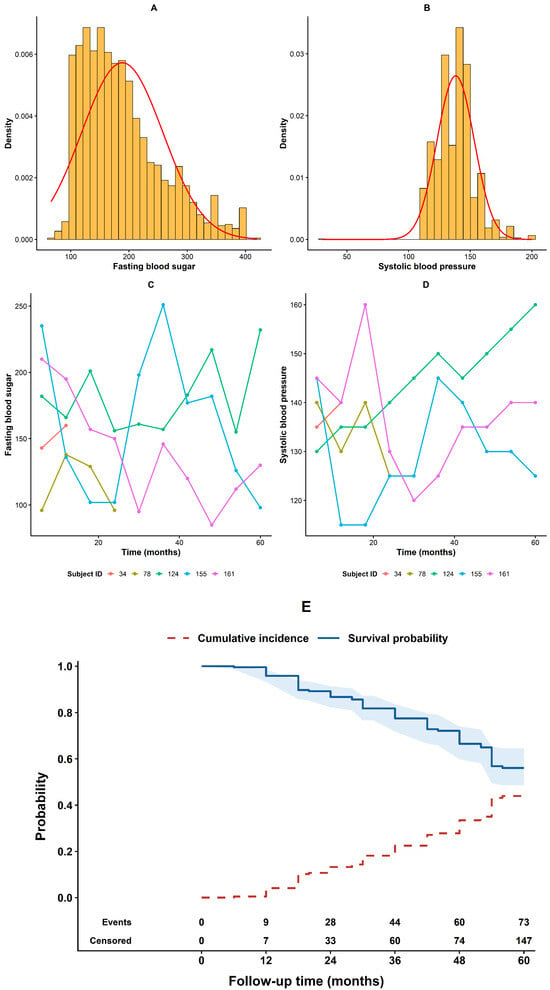
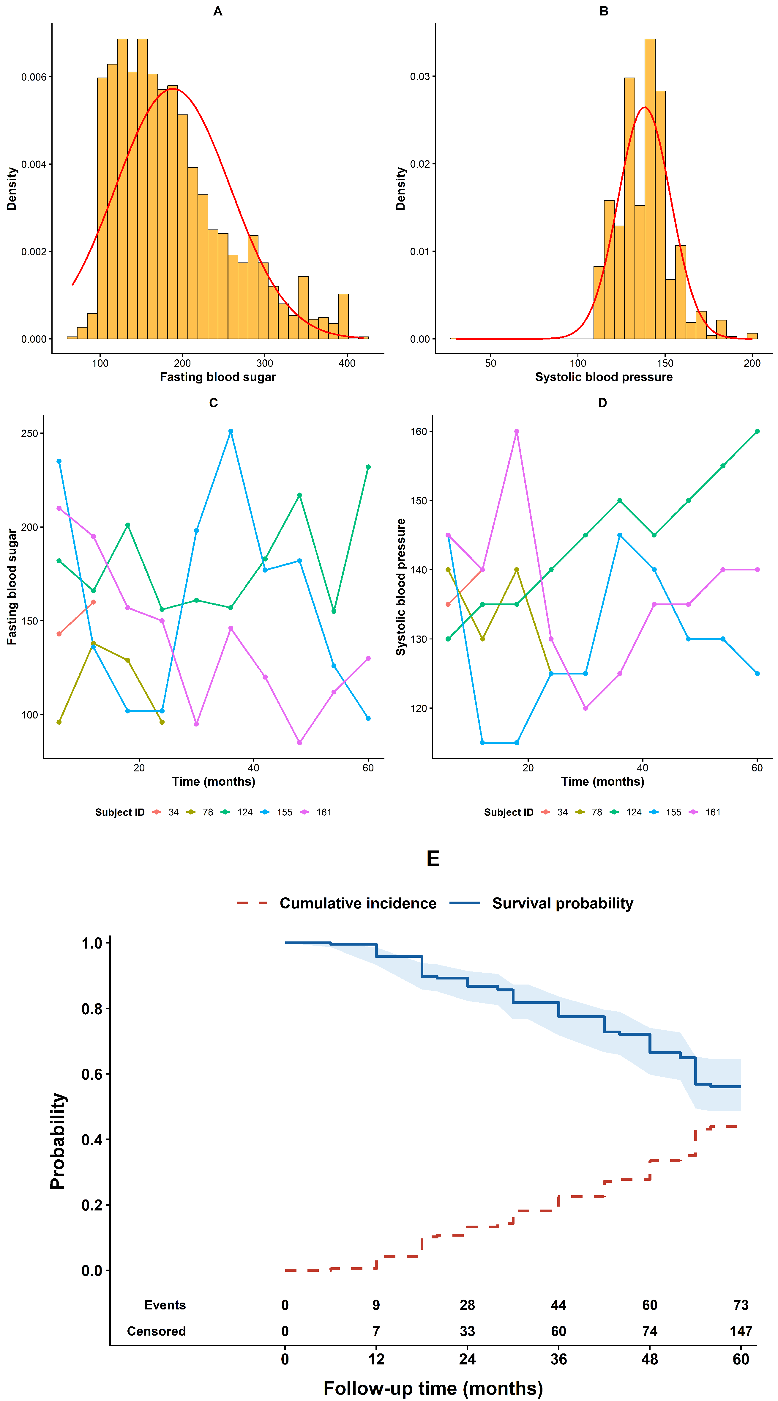
Figure 1A,B present histograms of FBS and SBP. As shown in these graphs, the distributions of SBP and FBS deviate from normality and are positively skewed. Figure 1C,D display SBP and FBS trajectories for five randomly selected patients, and these trajectories clearly demonstrate fluctuations over time. The survival and cumulative incidence functions depict the progression of time to the onset of chronic complications. It indicates that the cumulative incidence of chronic complications among individuals with T2D and hypertension is 28 individuals at 24 months, 44 individuals at 32 months, 60 individuals at 48 months, and 73 individuals at 60 months. As shown in the figure, the cumulative incidence is rising sharply at each follow-up time. We are mainly focused on how the cumulative incidence of chronic complications presented in Figure 1E is influenced by the trajectories of FBS and SBP (Figure 1C,D).

Figure 1. Exploratory plots of longitudinal and survival data in people with T2D and hypertension. Plots (A,B) are histograms of FBS and SBP with a normal curve that shows an asymmetric (right-skewed) distribution. Plots (C,D) display the longitudinal trajectories of fasting blood sugar and systolic blood pressure for five randomly selected subjects, while Plot (E) presents the Kaplan–Meier survival curve and the corresponding estimated cumulative incidence of chronic complications.

2.5. Model Implementation

The study presents a multivariate joint modeling approach that incorporates FBS and SBP as correlated longitudinal outcomes, with time to chronic complications as the event outcome. The multivariate linear mixed-effects model incorporates covariates such as measurement time (time), age, residence (0 = urban, 1 = rural), and sex (0 = male, 1 = female). As shown in Equation (1), the multivariate linear mixed-effects model is specified as follows:

$$Y_{ijk}=({\beta }_{1k}+b_{ik1})+({\beta }_{2k}+b_{ik2}){\mathrm{time}}_{ijk}+{\beta }_{3k}{\mathrm{age}}_i+{\beta }_{4k}{\mathrm{sex}}_i+{\beta }_{5k}{\mathrm{residence}}_i+e_{ijk}$$

(7)

where, $k=1$ and 2 represent FBS (mg/dL) and SBP (mmHg), respectively, for the $i^{\mathrm{th}}$ subject, measured at time $t_{ij}$, where $i=1,2,\dots ,220$ and $j=0,6,12,\dots ,54$. The fixed-effect parameter vector is ${\beta }^T={({\beta }_{11},{\beta }_{21},{\beta }_{31},{\beta }_{41},{\beta }_{51},{\beta }_{12},{\beta }_{22},{\beta }_{32},{\beta }_{42},{\beta }_{52})}^T$, denoting the intercept and the effects of time, age, sex, and residence on FBS and SBP. The random-effect vector is $b_i={(b_{i11},b_{i21},b_{i12},b_{i22})}^T$, denoting the random intercepts and random slopes. The $e_{ijk}$ are the random errors for FBS and SBP, respectively.

Chronic complications are the events of interest for the time-to-event outcomes. A study subject may either be under follow-up at the end of the study period or lose follow-up during the study period, which is considered right censoring $\left(C_i\right)$. Alternatively, during the study period, the subject may develop chronic complications at any time $T_i^{*}$. Then, for each study subject, the observed event time $\left(T_i\right)$ would be a $\min (T_i^{*},C_i)$. Body mass index (BMI), age, triglycerides, low-density lipoprotein (LDL), and high-density lipoprotein (HDL) were included as predictors of the time to occurrence of chronic complications. The time to onset of chronic complications can be modeled using a Cox regression model as follows:

$$\begin{array}{cc}\hfill \lambda (t\mid {\mathbf{X}}_i,{\mathbf{b}}_i)=& {\lambda }_0\left(t\right)\exp ({\gamma }_1{b}_{i11}+{\gamma }_2{b}_{i21}+{\gamma }_3{b}_{i12}+{\gamma }_4{b}_{i22}\hfill \\ \hfill & +{\alpha }_1{\mathrm{age}}_i+{\alpha }_2{\mathrm{BMI}}_i+{\alpha }_3{\mathrm{HDL}}_i\hfill \\ \hfill & +{\alpha }_4{\mathrm{LDL}}_i+{\alpha }_5{\mathrm{Triglyceride}}_i).\hfill \end{array}$$

(8)

where $\lambda (t\mid {\mathbf{X}}_i,{\mathbf{b}}_i)$ denotes the conditional hazard of chronic complications at time t, and ${\lambda }_0\left(t\right)$ is the baseline hazard function corresponding to zero values of the covariates and random effects. The parameter vector $\mathit{\gamma }={({\gamma }_1,{\gamma }_2,{\gamma }_3,{\gamma }_4)}^{\top }$ represents the associations between the subject-specific random intercepts and slopes of FBS and SBP and the hazard of chronic complications, whereas $\mathit{\alpha }={({\alpha }_1,{\alpha }_2,{\alpha }_3,{\alpha }_4,{\alpha }_5)}^{\top }$ represents the associations of age, BMI, HDL, LDL, and triglycerides with the hazard of chronic complications.

The longitudinal outcome variables of FBS and SBP exhibit a skewed multivariate normal distribution, as shown in Figure 1A,B. Consequently, multivariate linear mixed-effects models that assume a multivariate normal distribution for the random error could result in inaccurate parameter estimates [6,18]. Thus, we examine how skewness in the distribution of model errors affects the precision of parameter estimation by comparing two models.

• Model- Normal: Model with a multivariate normal distribution for both random errors and random effects.
• Model- skew Normal: Model with a multivariate skew-normal distribution for the random errors and a multivariate normal distribution for the random effects.

To carry out the Bayesian inference process, we must assign specific values to the hyperparameters in the prior distribution’s Equation (4). Vague priors with large variances were specified for all parameters in both the longitudinal and survival models. The fixed-effects vectors $\beta$, $\gamma$, and $\alpha$, as well as the skewness parameter $\Delta$, follows independent normal distribution with mean zero and variance 100, i.e., $N(0,100)$. The variance–covariance matrices of the random effects, ${\Sigma }_b$, and random errors, ${\Sigma }_k$, follow inverse Wishart distribution with ${\mathrm{\Omega }}_{{\Delta }_{bk}}=\mathrm{diag}(0.01,0.01,0.01,0.01)$ and 5 degrees of freedom, and ${\mathrm{\Omega }}_{{\Delta }_{ek}}=\mathrm{diag}(0.01,0.01)$ and 3 degrees of freedom, respectively.

Statistical analyses were conducted using the R software (version 4.6.0), with Bayesian estimation performed in JAGS through the bugs() function of the R2jags package. Convergence of the MCMC chains was assessed using graphical diagnostics, including trace plots and posterior density plots, as well as the Gelman–Rubin convergence diagnostic [19].

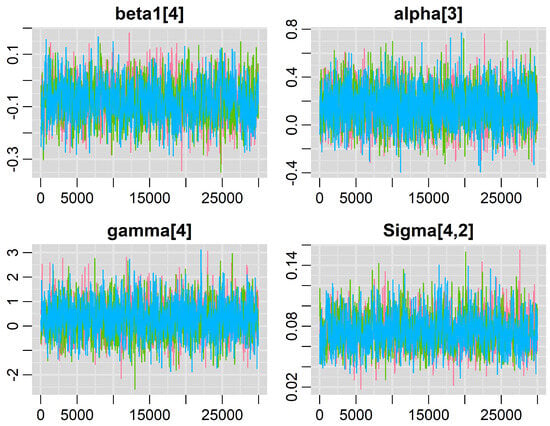
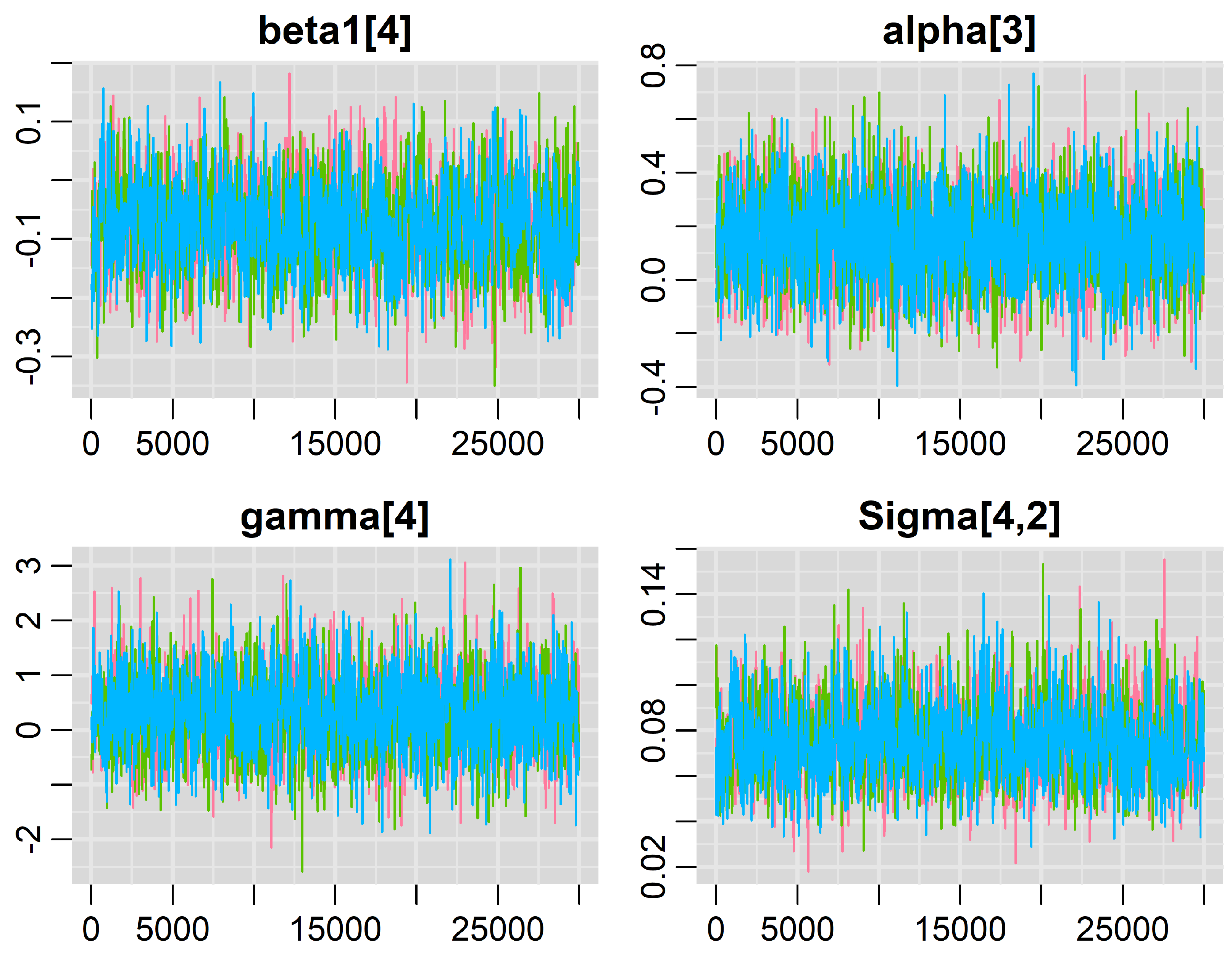
We ran three MCMC chains, each with 40,000 iterations, using the default randomly generated initial values. We discarded the first 10,000 iterations as burn-in and retained every 20th sample thereafter. Thus, we obtained 4500 posterior samples, which we used to draw statistical inferences. Figure 2 displays trace plots for selected regression coefficients. The trace plots show that the lines from the three chains are well mixed, indicating that the algorithm has converged.

Figure 2. Trace plots for selected parameters under the skew-normal model.

MCMC convergence was assessed using the Gelman–Rubin diagnostic ($\widehat{R}$), effective sample size (ESS), and Monte Carlo standard error (MCSE), as summarized in Table 2. The reported $\widehat{R}$ values ranged from approximately 1.001 to 1.035, suggesting no major convergence problems according to this diagnostic. However, several parameters had relatively low effective sample sizes, with the smallest ESS being 240, indicating that the Monte Carlo precision may be limited for some parameter estimates. Therefore, although the convergence diagnostics provide reasonable support for the stability of the MCMC results, the posterior estimates should be interpreted with appropriate caution.

Table 2. Results of the Gelman–Rubin convergence diagnostic ($\hat{R}$), effective sample size (ESS), and Monte Carlo standard error (MCSE) for each parameter.

Parameter	$\widehat{\mathit{R}}$	ESS	MCSE
${\beta }_{11}$	1.035	240	0.0030
${\beta }_{21}$	1.031	690	0.0010
${\beta }_{31}$	1.017	270	0.0019
${\beta }_{41}$	1.005	2000	0.0013
${\beta }_{51}$	1.007	530	0.0028
${\beta }_{12}$	1.009	510	0.0025
${\beta }_{22}$	1.035	3300	0.0005
${\beta }_{32}$	1.009	4400	0.0005
${\beta }_{42}$	1.008	270	0.0046
${\beta }_{52}$	1.006	340	0.0041
${\alpha }_1$	1.001	4500	0.0016
${\alpha }_2$	1.002	860	0.0055
${\alpha }_3$	1.006	4500	0.0019
${\alpha }_4$	1.002	2200	0.0031
${\alpha }_5$	1.002	3300	0.0024
${\gamma }_1$	1.016	600	0.0220
${\gamma }_2$	1.011	4500	0.0110
${\gamma }_3$	1.001	590	0.0129
${\gamma }_4$	1.003	760	0.0260
$v_{11}$	1.003	340	0.0016
$v_{22}$	1.004	580	0.0005
$v_{33}$	1.0042	820	0.0011
$v_{44}$	1.003	1000	0.0006
$v_{12}$	1.004	680	0.0005
$v_{13}$	1.010	460	0.0009
$v_{14}$	1.003	460	0.0007
$v_{23}$	1.005	660	0.0005
$v_{34}$	1.005	710	0.0007
${\delta }_1$	1.002	680	0.0011
${\delta }_2$	1.002	600	0.0018

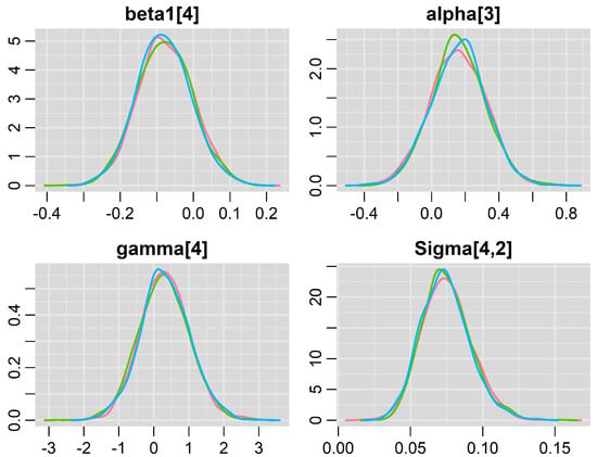
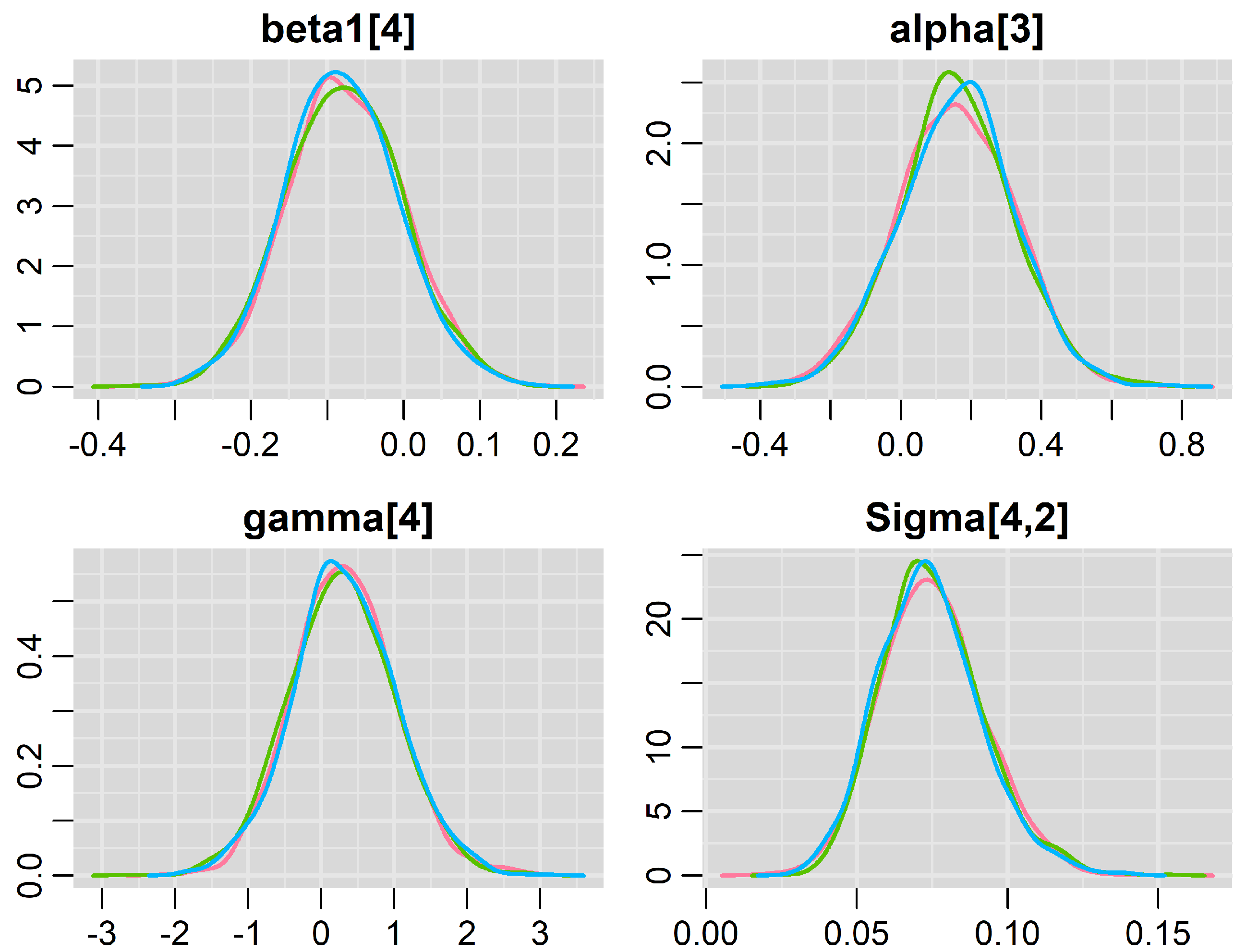
Additionally, the posterior density plots in Figure 3 offer valuable insights: the density plots from each chain closely overlap and have the same shape, indicating that the algorithm has converged.

Figure 3. Posterior density plots for selected parameters under the skew-normal model.

3. Data Analysis and Results

To reduce variability from measurement errors and improve the efficiency of the estimation algorithm, the longitudinal data for SBP and FBS are standardized. The quantitative covariates are also standardized to avoid unstable estimates. Consequently, the results are expressed in standard units rather than in the original measurement units.

In the multivariate linear mixed-effects model, the estimated random-effect covariance parameters provide information about the variability and dependence structure of the longitudinal FBS and SBP trajectories, as presented in Table 3. Under the skew-normal model, the estimated covariance between the FBS random intercept and the SBP random intercept was 0.074, while the covariance between their random slopes was 0.040. Both estimates were positive, and their corresponding 95% credible intervals excluded zero, suggesting positive posterior associations between the corresponding subject-specific random effects. The estimated within-outcome covariances between random intercepts and slopes were also positive for FBS (0.071) and SBP (0.060). These findings indicate a positive dependence structure among the modeled random effects. However, because these parameters represent covariances rather than correlations, their magnitudes should not be interpreted directly as measures of correlation strength without appropriate standardization.

Table 3. Summary of the estimated posterior mean (PM) of variance–covariance matrix parameters for random errors and random effects, standard deviation (SD), and 95% credible intervals (CI) for each model.

Parameter	Model-Normal			Model-Skew Normal
	PM	SD	95% CI	PM	SD	95% CI
${\sigma }_{11}^2$	0.603	0.023	0.559, 0.649	0.034	0.006	0.029, 0.049
${\sigma }_{22}^2$	0.652	0.025	0.606, 0.702	0.592	0.027	0.549, 0.653
${\sigma }_{12}^2$	0.206	0.017	0.173, 0.241	0.021	0.015	0.011, 0.051
$v_{11}$	0.288	0.040	0.218, 0.372	0.167	0.023	0.151, 0.215
$v_{22}$	0.144	0.023	0.104, 0.194	0.075	0.013	0.065, 0.104
$v_{33}$	0.239	0.036	0.214, 0.315	0.219	0.031	0.198, 0.286
$v_{44}$	0.126	0.020	0.112, 0.169	0.110	0.018	0.097, 0.149
$v_{12}$	0.108	0.022	0.093, 0.155	0.071	0.013	0.061, 0.099
$v_{13}$	0.121	0.020	0.091, 0.169	0.074	0.019	0.061, 0.115
$v_{14}$	0.107	0.022	0.091, 0.152	0.079	0.015	0.068, 0.111
$v_{23}$	0.058	0.021	0.044, 0.101	0.035	0.014	0.026, 0.064
$v_{34}$	0.073	0.019	0.059, 0.112	0.060	0.018	0.048, 0.097
$v_{24}$	0.075	0.019	0.037, 0.086	0.040	0.019	0.034, 0.109

Table 4 presents the posterior means, standard deviations (SD), and 95% credible intervals for all parameters from the multivariate joint model, accounting for the distribution of random errors.

Table 4. Posterior mean, standard deviation (SD), and 95% credible intervals (CI) for parameters under model normal and model skew-normal.

Parameter	Model Normal			Model Skew Normal
	Posterior Mean	SD	95% CI	Posterior Mean	SD	95% CI
Multivariate linear mixed-effects model parameters estimates
${\beta }_{11}$	0.008	0.058	(−0.104, 0.121)	0.022	0.046	(−0.073, 0.112)
${\beta }_{21}$	0.071	0.033	(0.006, 0.138)	0.041	0.027	(−0.012, 0.095)
${\beta }_{31}$	0.045	0.037	(−0.026, 0.117)	0.028	0.031	(−0.021, 0.116)
${\beta }_{41}$	−0.078	0.075	(−0.224, 0.072)	0.011	0.056	(−0.100, 0.116)
${\beta }_{51}$	0.120	0.079	(−0.032, 0.275)	0.018	0.064	(−0.062, 0.131)
${\beta }_{12}$	0.030	0.057	(−0.083, 0.145)	0.028	0.056	(−0.095, 0.121)
${\beta }_{22}$	0.067	0.032	(0.006, 0.131)	0.055	0.031	(0.003, 0.125)
${\beta }_{32}$	0.112	0.037	(0.043, 0.185)	0.107	0.035	(0.042, 0.182)
${\beta }_{42}$	−0.078	0.076	(−0.226, 0.066)	−0.042	0.076	(−0.197, 0.095)
${\beta }_{52}$	0.045	0.077	(−0.107, 0.191)	0.012	0.076	(−0.115, 0.176)
${\delta }_1$				1.285	0.029	(1.266, 1.342)
${\delta }_2$				0.423	0.044	(0.393, 0.509)
Survival model parameters estimates
${\gamma }_1$	0.239	0.425	(−0.603, 1.083)	−0.620	0.540	(−1.217, 0.912)
${\gamma }_2$	−0.510	0.609	(−1.781, 0.622)	−0.027	0.740	(−1.834, 1.047)
${\gamma }_3$	0.283	0.320	(−0.362, 0.917)	0.234	0.314	(−0.348, 0.886)
${\gamma }_4$	0.312	0.709	(−1.054, 1.731)	0.520	0.717	(−0.978, 1.882)
${\alpha }_1$	0.038	0.109	(−0.178, 0.246)	0.026	0.107	(−0.181, 0.236)
${\alpha }_2$	0.159	0.162	(−0.162, 0.474)	0.220	0.161	(−0.112, 0.502)
${\alpha }_3$	0.042	0.130	(−0.215, 0.299)	0.007	0.129	(−0.232, 0.272)
${\alpha }_4$	−0.121	0.146	(−0.402, 0.171)	−0.081	0.147	(−0.383, 0.193)
${\alpha }_5$	−0.066	0.140	(−0.347, 0.212)	−0.029	0.139	(−0.145, 0.100)
DIC	9105.747			3738.161

In the multivariate linear mixed-effects submodel, the parameter estimates ($\beta$) under the model normal are slightly higher than those under the model skew normal. There are some differences in the magnitude of the coefficient ($\alpha$) between the two models, and there is substantial variation in the estimates of the association parameter ($\gamma$). This is particularly evident for the random intercept and slope for FBS. These results indicate substantial variation in the estimated association parameter for longitudinal and time-to-event data under different distributional assumptions for the random errors.

The Deviance Information Criterion (DIC), as proposed by [20], is used to select the model that best fits the data. Like other model selection criteria, it is important to note that DIC is not intended to identify the “correct” model but rather to facilitate comparisons among models that provide a reasonable fit to the data. Table 4 summarizes the DIC values for the two models. The model skew normal provides a better fit to the data, as its DIC value is smaller than that of the other model. Therefore, the multivariate joint model with multivariate skew-normal random errors is used for subsequent interpretation and discussion.

Under the skew-normal model, the estimated skewness parameters were positive for both FBS (${\delta }_1=1.285$; 95% credible interval: 1.266–1.342) and SBP (${\delta }_2=0.423$; 95% credible interval: 0.393–0.509), as shown in Table 4. These results provide evidence of positive asymmetry in the modeled longitudinal error distributions. The skew-normal model also yielded a lower DIC than the normal model, suggesting a better relative fit, provided that the DIC values were computed using comparable likelihood definitions. Regarding the longitudinal fixed effects, the estimated effects of measurement time and age on SBP were positive, with 95% credible intervals excluding zero. For FBS, the corresponding posterior mean estimates were also positive, but their 95% credible intervals included zero. Although the estimated residence and sex effects varied in direction and magnitude, their 95% credible intervals included zero under the skew-normal model. Therefore, the data do not provide conclusive evidence of differences in longitudinal FBS or SBP trajectories by residence or sex after accounting for the other modeled variables.

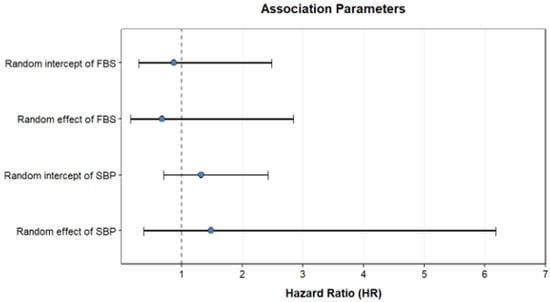
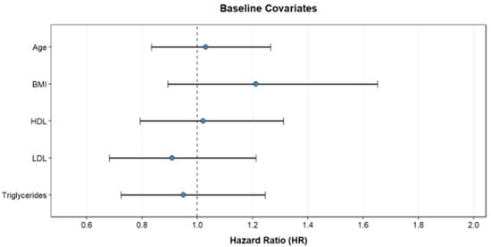
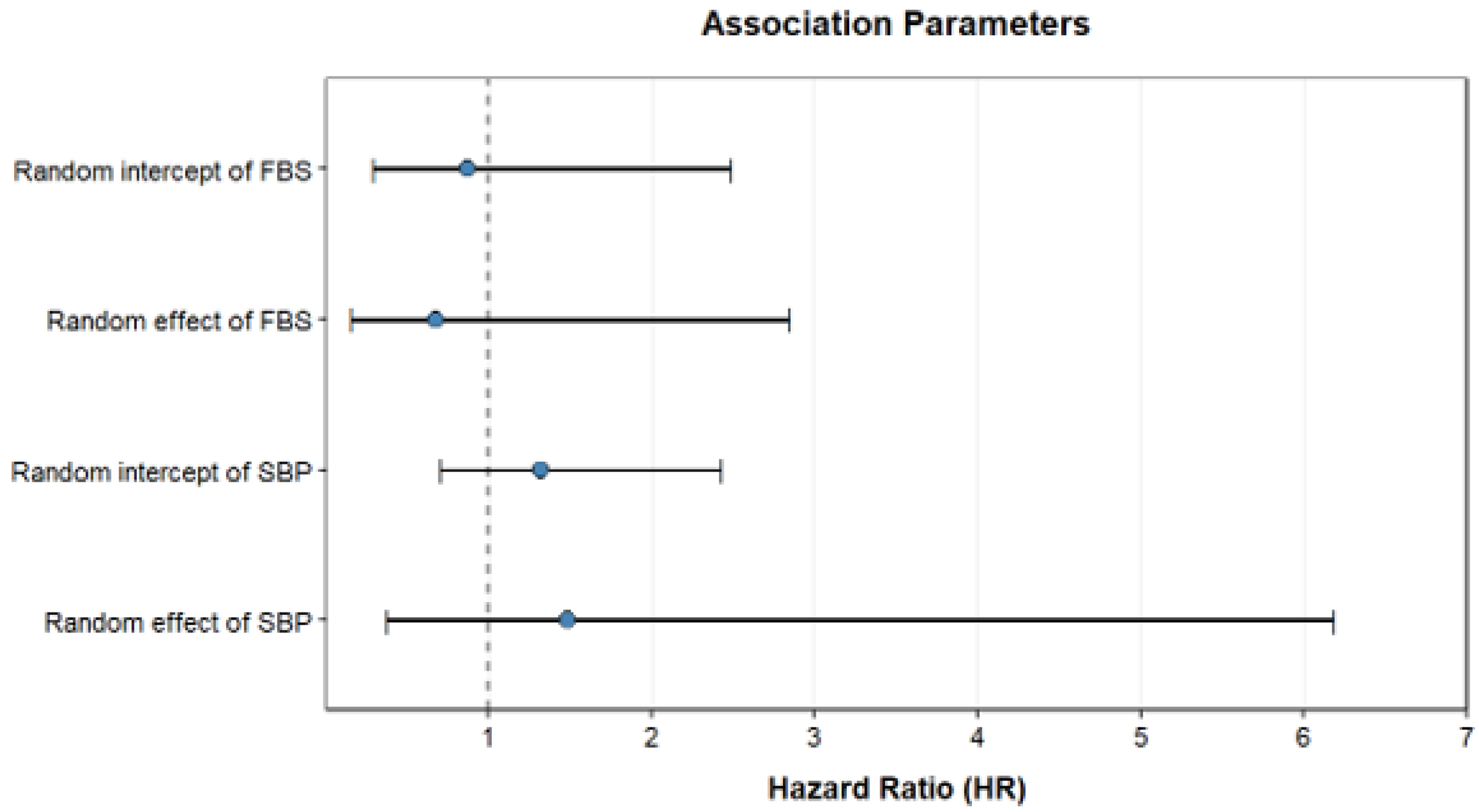
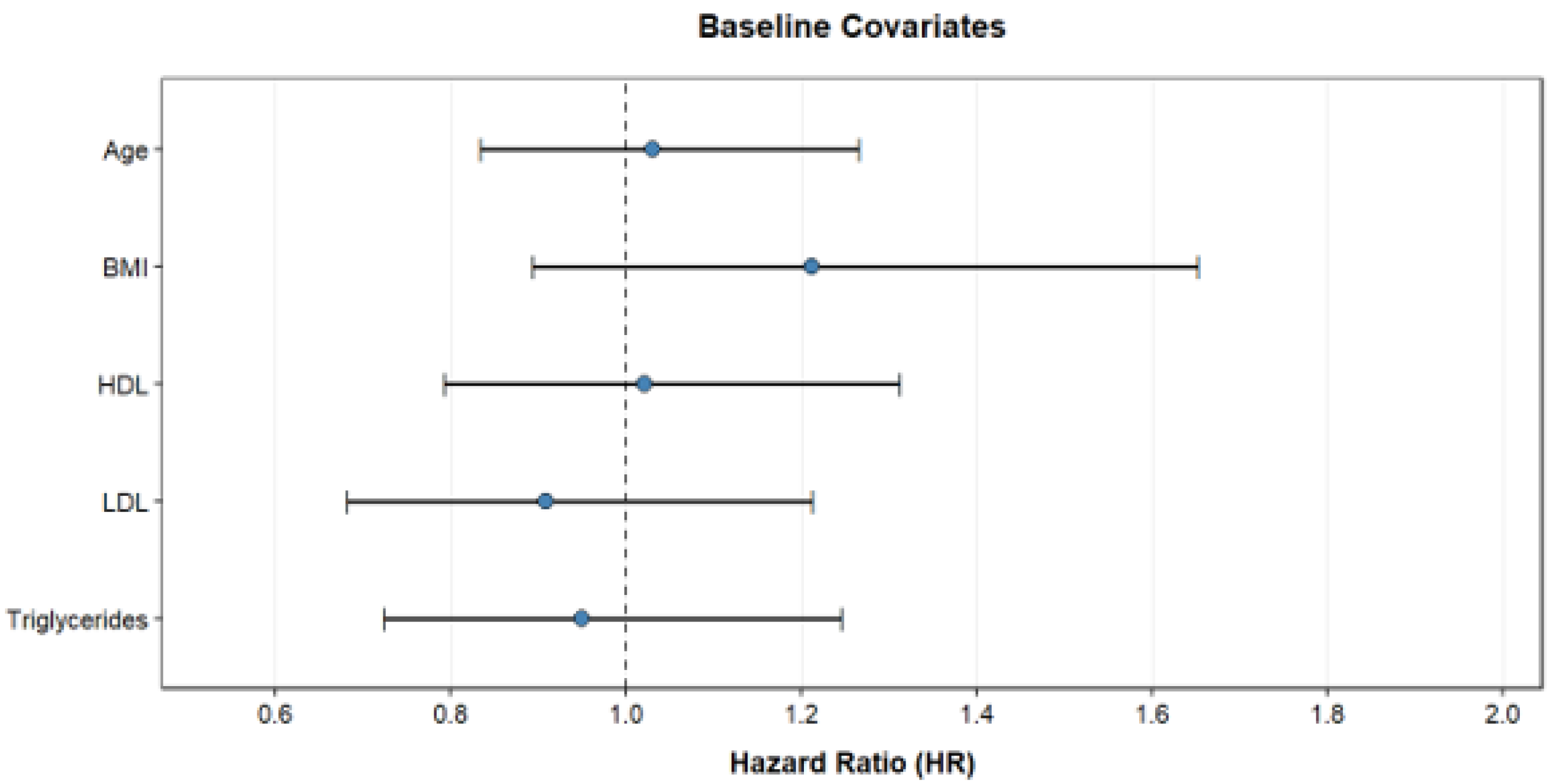
The estimated parameters $\alpha$ and $\gamma$ in the results of the survival sub-model indicate how longitudinal measurements, clinical and biochemical variables, influence the time to onset of chronic complications. The SBP random-intercept and random-slope association parameters are ${\gamma }_3$ and ${\gamma }_4$, respectively. The posterior mean for ${\gamma }_4$ is 0.520, corresponding to a conditional hazard ratio $\exp \left(0.520\right)=1.682$ for a one-unit increase in the SBP random-slope component, holding the other modeled quantities fixed. The reported 95% credible interval for ${\gamma }_4$, $(-0.978,1.882)$, transforms to an approximate hazard-ratio interval of $(0.376,6.567)$, which includes 1. Therefore, these data do not establish a positive SBP slope–hazard association. This effect should not be described as a one-unit increase in measured SBP or as a causal effect. Other covariate associations should likewise be interpreted in light of their credible intervals. Figure 4 illustrates the hazard ratio (HR), longitudinal effects of FBS and SBP, and covariates related to the risk of chronic complications.

Figure 4. Hazard ratio of the survival submodel based on the model skew-normal; longitudinal effects of FBS, SBP, and covariates on the risk of chronic complications.

3.1. Simulation Studies

We conducted limited simulation studies to compare the proposed multivariate joint model under different random error distributions and to assess how asymmetry in the longitudinal biomarker affects the results. The design of the simulated dataset was similar to the application using T2D and hypertension data. We generated two longitudinal outcomes, one time-to-event outcome, and covariates. Longitudinal measurements were taken twice per year, with a maximum follow-up of 5 years, and visit intervals were identical for all subjects. The multivariate, correlated longitudinal outcomes were generated using the multivariate linear mixed-effects submodel described in Equation (1). We set the true values of the model parameters to those obtained from the real data analysis for the model skew-normal, which are presented in Table 4. ${\beta }_1=({\beta }_{11},{\beta }_{21},{\beta }_{31},{\beta }_{41},{\beta }_{51})=(0.022,0.041,0.028,0.011,0.018)$, ${\beta }_2=({\beta }_{12},{\beta }_{22},{\beta }_{32},{\beta }_{42},{\beta }_{52})=(0.028,0.055,0.107,-0.042,0.012)$, $\gamma =({\gamma }_1,{\gamma }_2,{\gamma }_3,{\gamma }_4)=(-0.620,-0.027,0.234,0.520)$, and $\alpha =({\alpha }_1,{\alpha }_2,{\alpha }_3,{\alpha }_4,{\alpha }_5)=(0.026,0.220,0.007,-0.081,-0.029)$. The random-effects vector was simulated from a multivariate normal distribution with mean zero and a specified variance-covariance matrix; its values are shown in Table 3. For the longitudinal data, random errors for SBP and FBS were generated from a Gamma distribution with shape and scale parameters both equal to 1. The generated values were centered by subtracting their theoretical mean of 1, yielding zero-mean, positively skewed errors. Thus, the simulated errors followed a centered Gamma distribution rather than a skew-normal distribution. This design allowed us to assess the performance of the proposed skew-normal joint model under a non-normal, asymmetric data-generating mechanism. We simulated the time-to-event data using the proportional hazards model described in Equation (2). For each subject, survival time was simulated from an exponential distribution with a constant baseline hazard rate of 0.1. Censoring times were generated from an exponential distribution, independently of the simulated event times. The numerical censoring parameter is not specified here because its rate-versus-mean convention cannot be established from the available simulation description; the empirical censoring proportion is likewise unavailable. Event times were generated from an exponential distribution with a subject-specific rate that depends on the random-effects process for the longitudinal outcomes and the covariates. In contrast, the random censoring times was generated independently of the event times. We assume that censoring is noninformative, meaning that the censoring event does not depend on either the random-effects process for the longitudinal outcomes or the covariates. Let $C_i$ be the censoring time and let $T_i^{*}$ be the true event time. Thus, the observed survival time of the $i^{\mathrm{th}}$ subject was computed as $T_i=\min (T_i^{*},C_i).$ The event status for the $i^{\mathrm{th}}$ subject was denoted by

$${\tau }_i=\left\{\begin{array}{cc}1,\hfill & \mathrm{if}{T}_i^{*}\le C_i,\hfill \\ 0,\hfill & \mathrm{otherwise}.\hfill \end{array}\right.$$

The covariates included in both sub-models are mimicked from the real dataset and simulated based on variable types. For example, the qualitative covariates sex (with male as the reference) and residence (with urban as the reference) were simulated from Bernoulli distributions with success probabilities of 0.40 and 0.32, respectively. The continuous covariates were generated from a normal distribution, with parameter values chosen according to the application dataset.

Because of the extensive computation required, we simulated only 50 data sets, each with 150 subjects, to keep the study feasible. Although a larger number of replications and subjects is recommended for a more robust simulation study, in our case this would have required substantially more computation time, as analyzing each data set took over 2 h. Then each dataset is fitted with the model normal and model skew-normal to determine which model fits the data well and to identify which model provides a relatively unbiased parameter estimate. The Bayesian inference used to estimate the parameters of each model, including the specification of prior distributions and the convergence diagnostic tools, was similar to that used for the applied data set. To compare the performance of parameter estimates under the two models, we computed

$$\mathrm{RMSE}\left(\theta \right)=\sqrt{{\displaystyle \frac{1}{m}}\sum _{i=1}^m{\left({\widehat{\theta }}_i-{\theta }_T\right)}^2},$$

$$B\left(\theta \right)={\displaystyle \frac{1}{m}}{\displaystyle \sum _{i=1}^m}{\widehat{\theta }}_i-{\theta }_T,$$

and the DIC, where ${\widehat{\theta }}_i$ is the estimate of the true parameter ${\theta }_T$ from the $i^{\mathrm{th}}$ simulation, ${\theta }_T$ is the true parameter value obtained from the application data set, and m is the total number of replications.

Table 5 summarizes the simulation results for the two models, including the true parameter (TP) values, bias, and root-mean-square error (RMSE) for the fixed-effect parameters. Positive bias indicates overestimation of the corresponding true parameter, whereas negative bias indicates underestimation. The direction and magnitude of the reported biases vary across parameters and between the two models. Smaller absolute bias and RMSE values generally indicate more accurate estimation under the simulated conditions. However, the relative performance of the models should be evaluated across all parameters rather than on the basis of individual estimates alone.

Table 5. Summary of true parameter (TP) values, bias, and RMSE for the Model normal and model skew-normal.

Parameter	TP	Model Normal		Model Skew-Normal
		Bias	RMSE	Bias	RMSE
${\beta }_{11}$	0.022	−1.490	1.494	−1.490	1.494
${\beta }_{21}$	0.041	−0.006	0.087	−0.001	0.086
${\beta }_{31}$	0.028	−0.020	0.089	−0.014	0.087
${\beta }_{41}$	0.011	−0.031	0.180	−0.039	0.186
${\beta }_{51}$	0.018	−0.030	0.214	−0.020	0.218
${\beta }_{12}$	0.028	−1.242	1.429	−1.286	1.293
${\beta }_{22}$	0.055	−0.009	0.094	−0.001	0.104
${\beta }_{32}$	0.107	−0.023	0.093	−0.026	0.100
${\beta }_{42}$	−0.042	0.043	0.195	0.021	0.197
${\beta }_{52}$	0.012	0.024	0.236	0.020	0.236
${\gamma }_1$	−0.620	0.001	0.298	0.000	0.296
${\gamma }_2$	−0.027	−0.039	0.257	−0.034	0.265
${\gamma }_3$	0.234	0.066	0.342	0.012	0.252
${\gamma }_4$	0.520	−0.522	0.820	−0.068	0.314
${\alpha }_1$	0.026	0.070	0.274	0.069	0.276
${\alpha }_2$	0.220	0.062	0.282	0.062	0.273
${\alpha }_3$	0.007	0.033	0.275	0.030	0.266
${\alpha }_4$	−0.081	−0.046	0.224	−0.038	0.224
${\alpha }_5$	−0.029	0.015	0.234	0.014	0.232
DIC	7369			6600

The simulation results showed differences in estimation performance between the normal and skew-normal models. The skew-normal model produced smaller absolute biases and RMSE values for several parameters, particularly some of the survival association parameters. However, these improvements were not uniform across all parameters. The lower DIC obtained for the skew-normal model suggests a better relative fit under the simulated conditions, provided that the DIC values were computed on a comparable basis. Overall, these findings provide preliminary evidence that accommodating asymmetric random errors may improve model performance in certain settings, although broader simulation studies are needed to establish the generality of these results.

3.2. Discussion

As more studies are conducted, collecting repeated measurements over time becomes increasingly important for evaluating human health with joint models for longitudinal and time-to-event data. However, most existing joint modeling analyses rely on a univariate framework with a single time-to-event outcome and a single longitudinal outcome, and they assume that the random errors follow a normal distribution. Motivated by hypertension and diabetes, this study extends univariate joint models to multivariate joint models by accounting for the skewness of the longitudinal outcomes SBP and FBS. The two submodels are linked through shared random effects to assess the relationship between the longitudinal and time-to-event processes.

We compared two multivariate joint models with different distributional assumptions for the longitudinal random errors. The first model assumed multivariate normal distributions for both the random effects and random errors, whereas the second model incorporated multivariate skew-normal random errors while retaining normally distributed random effects. Under the skew-normal model, the estimated skewness parameters for FBS and SBP were positive, providing evidence of asymmetry in the modeled longitudinal error distributions. The skew-normal model yielded a lower DIC in the application, suggesting improved relative fit if the DIC values were computed on a comparable basis. The simulation results also indicated smaller absolute biases and RMSE values for some parameters under the skew-normal model, although these improvements were not consistent across all parameters. Overall, these findings suggest that accommodating asymmetric longitudinal errors may be beneficial in multivariate joint modeling. However, the limited simulation design does not establish uniform superiority of the skew-normal model across different data-generating mechanisms. Previous studies [21,22] have also investigated flexible distributional assumptions in joint modeling, providing relevant methodological context for the present findings.

When we consider the clinical implications, the overall incidence of chronic complications in people with T2D and hypertension was 33.20% over the five-year study period. These findings are similar to previous research in Bahir Dar, Ethiopia (32.4% over seven years) [23], Gondar, Ethiopia (28% during a follow-up of 6 years) [24] and Wollega, Ethiopia (31.2%) [25]. There is a strong association between changes in FBS and SBP in individuals with T2D and hypertension. Although previous studies have linked elevated FBS and SBP to adverse clinical outcomes, the estimated associations between the subject-specific biomarker trajectories and the hazard of chronic complications in our analysis were subject to substantial posterior uncertainty. Previous studies have reported associations between blood pressure variability and adverse clinical outcomes [26,27]. Although our findings do not establish a statistically conclusive association between the longitudinal biomarker trajectories and the hazard of chronic complications, they support the importance of investigating FBS and SBP jointly in future studies.

Among the covariates included in the proportional hazards submodel, the posterior mean estimates for age, BMI, and HDL were positive, whereas those for triglycerides and LDL were negative. However, the corresponding 95% credible intervals included zero for all five covariates, indicating substantial posterior uncertainty regarding the direction and magnitude of these associations. Consequently, our findings do not provide conclusive evidence of an association between these individual covariates and the hazard of chronic complications after accounting for the other variables in the joint model. Previous studies [28,29] have investigated the relationships between clinical and lipid-related factors and diabetes-related complications. Although these studies provide relevant clinical context, differences in study populations, outcomes, and statistical methodologies limit direct comparisons with our findings.

Our results illustrate the potential clinical relevance of jointly examining SBP and FBS trajectories in relation to the risk of chronic complications among individuals with T2D and hypertension. Although the estimated association between the SBP random-slope component and the hazard of chronic complications was positive, its 95% credible interval included zero, indicating substantial uncertainty regarding the direction and magnitude of this association. Therefore, these findings should not be interpreted as conclusive evidence that increasing SBP trajectories are associated with a higher risk of chronic complications. The estimated associations involving FBS should likewise be interpreted in light of their posterior uncertainty. Nevertheless, the proposed joint modeling framework provides a unified approach for examining the relationships between multiple correlated longitudinal biomarkers and time-to-event outcomes while accounting for their underlying dependence structure. This framework allows the simultaneous assessment of repeated biomarker measurements and their potential associations with the timing of chronic complications.

Our findings regarding SBP can be considered in the context of previous studies examining associations between blood pressure and cardiovascular or diabetes-related complications. Li et al. [30] reported a 1.70-fold increase in the risk of heart failure for each standardized unit increase in SBP. Similarly, Ceriello et al. [31] found that patients with high variability in both body weight and blood pressure had an elevated risk of cardiovascular disease (HR = 1.81; 95% confidence interval: 1.61–2.05) compared with patients with low variability in both body weight and total cholesterol. Furthermore, Dorajoo et al. [32] investigated the association between HbA1c variability and new-onset albuminuria among patients with type 2 diabetes. Although these studies provide evidence of associations between longitudinal biomarker measures and adverse clinical outcomes, direct comparisons with our findings are limited by differences in predictors, endpoints, and statistical models. In our analysis, the estimated association between the SBP random-slope component and the hazard of chronic complications was positive, although its 95% credible interval included zero, indicating substantial uncertainty regarding the direction and magnitude of the association. Therefore, our results do not provide conclusive evidence of a positive association. Moreover, because these estimates are based on observational data, they should not be interpreted as establishing a causal relationship between SBP trajectories and the risk of chronic complications.

This study has limitations that should be acknowledged. First, the survival submodel considers a single event type, whereas individuals with T2D and hypertension may experience different types of chronic complications. Future extensions could incorporate competing-risks survival models to account for multiple event types [1,7,30]. Second, the longitudinal submodel assumes linear trajectories over time for FBS and SBP. Although this assumption provides a parsimonious representation of the longitudinal processes, the underlying biomarker trajectories may exhibit nonlinear patterns that cannot be fully captured by a linear mixed-effects model [10]. If such nonlinearity is present, the assumed linear trajectories may lead to model misspecification and affect the estimated associations between the longitudinal biomarkers and the hazard of chronic complications. A possible extension would be to incorporate flexible semiparametric mixed-effects models with nonparametric smoothing functions of time. Third, the application was based on a relatively small sample of 220 individuals, with 73 observed events, which may limit the precision and stability of the parameter estimates. Furthermore, sensitivity analyses were not conducted to evaluate the effects of sample size, number of observed events, alternative association structures, or varying degrees of skewness on model performance. Future research should address these limitations through more extensive simulation studies and applications to larger datasets, while exploring flexible longitudinal trajectories and competing-risks extensions of the proposed joint modeling framework.

4. Conclusions

We proposed a Bayesian joint model for multivariate longitudinal and time-to-event data that simultaneously accommodates multiple correlated longitudinal biomarkers and survival outcomes while relaxing the multivariate normality assumption by using a multivariate skew normal distribution for the random errors. By jointly modeling multiple longitudinal processes with shared random effects, the proposed framework effectively addresses within-subject correlation, between-outcome dependence, and asymmetric longitudinal measurements within a unified inferential structure.

The limited simulation study revealed differences in estimation performance between the normal and skew-normal models. Although the skew-normal model yielded smaller absolute biases and RMSE values for some parameters, these improvements were not uniform across all parameters, and the limited simulation design does not establish general superiority. In the motivating application involving individuals with T2D and hypertension, the proposed framework jointly modeled the longitudinal trajectories of FBS and SBP and their associations with the time to chronic complications. The estimated association between the SBP random-slope component and the hazard of chronic complications was positive. However, its 95% credible interval included zero, indicating substantial posterior uncertainty regarding the direction and magnitude of this association. Thus, the application illustrates the utility of the proposed framework without establishing a definitive association between increasing SBP trajectories and the risk of chronic complications.

Although motivated by a diabetes and hypertension study, the proposed methodology is broadly applicable to biomedical and epidemiological research involving multiple correlated longitudinal biomarkers and time-to-event outcomes. The framework provides a flexible extension of existing Bayesian joint models for settings in which the Gaussian assumption is unrealistic. Future research may extend the proposed model to accommodate multiple survival outcomes, competing risks, recurrent events, high-dimensional biomarkers, and more flexible distributional assumptions, including skew-t and nonparametric Bayesian formulations.

References

- Hu, W.; Li, G.; Li, N. A Bayesian approach to joint analysis of longitudinal measurements and competing risks failure time data. Stat. Med. 2009, 28, 1601–1619. [Google Scholar] [CrossRef] [Scilit] [PubMed]
- Ibrahim, J.G.; Chu, H.; Chen, L.M. Basic concepts and methods for joint models of longitudinal and survival data. J. Clin. Oncol. 2010, 28, 2796–2801. [Google Scholar] [CrossRef] [Scilit] [PubMed]
- Lawrence Gould, A.; Boye, M.E.; Crowther, M.J.; Ibrahim, J.G.; Quartey, G.; Micallef, S.; Bois, F.Y. Joint modeling of survival and longitudinal non-survival data: Current methods and issues. Report of the DIA Bayesian joint modeling working group. Stat. Med. 2015, 34, 2181–2195. [Google Scholar] [CrossRef] [Scilit] [PubMed]
- Andrinopoulou, E.R.; Rizopoulos, D.; Takkenberg, J.J.; Lesaffre, E. Combined dynamic predictions using joint models of two longitudinal outcomes and competing risk data. Stat. Methods Med. Res. 2017, 26, 1787–1801. [Google Scholar] [CrossRef] [Scilit] [PubMed]
- Crowther, M.J.; Abrams, K.R.; Lambert, P.C. Joint modeling of longitudinal and survival data. Stata J. 2013, 13, 165–184. [Google Scholar] [CrossRef] [Scilit]
- Huang, Y.; Chen, J.; Xu, L.; Tang, N.S. Bayesian Joint Modeling of Multivariate Longitudinal and Survival Data with an Application to Diabetes Study. Front. Big Data 2022, 5, 812725. [Google Scholar] [CrossRef] [Scilit] [PubMed]
- Ferede, M.M.; Mwalili, S.; Dagne, G.; Karanja, S.; Hailu, W.; El-Morshedy, M.; Al-Bossly, A. A semiparametric Bayesian joint modelling of skewed longitudinal and competing risks failure time data: With application to chronic kidney disease. Mathematics 2022, 10, 4816. [Google Scholar] [CrossRef] [Scilit]
- Yewhalaw, D.; Getachew, Y.; Tushune, K.; W/Michael, K.; Kassahun, W.; Duchateau, L.; Speybroeck, N. The effect of dams and seasons on malaria incidence and anopheles abundance in Ethiopia. BMC Infect. Dis. 2013, 13, 161. [Google Scholar] [CrossRef] [Scilit] [PubMed]
- Bandyopadhyay, D.; Lachos, V.H.; Abanto-Valle, C.A.; Ghosh, P. Linear mixed models for skew-normal/independent bivariate responses with an application to periodontal disease. Stat. Med. 2010, 29, 2643–2655. [Google Scholar] [CrossRef] [Scilit] [PubMed]
- Mekonen, M.W.; Alibrandi, A.; Asfaw, T.W.; Kifle, Y.G.; Konietschke, F.; Asfaw, Z.G. A Flexible Bayesian Semi-Parametric Multivariate Mixed-Effect Model Framework for Skewed Longitudinal Data. Mathematics 2026, 14, 2030. [Google Scholar] [CrossRef] [Scilit]
- Sahu, S.K.; Dey, D.K.; Branco, M.D. A new class of multivariate skew distributions with applications to Bayesian regression models. Can. J. Stat. 2003, 31, 129–150. [Google Scholar] [CrossRef] [Scilit]
- Arellano-Valle, R.B.; Bolfarine, H.; Lachos, V.H. Bayesian inference for skew-normal linear mixed models. J. Appl. Stat. 2007, 34, 663–682. [Google Scholar] [CrossRef] [Scilit]
- Huang, Y.; Dagne, G. Skew-normal Bayesian nonlinear mixed-effects models with application to AIDS studies. Stat. Med. 2010, 29, 2384–2398. [Google Scholar] [CrossRef] [Scilit] [PubMed]
- Ferede, M.M.; Dagne, G.A.; Mwalili, S.M.; Bilchut, W.H.; Engida, H.A.; Karanja, S.M. Flexible Bayesian semiparametric mixed-effects model for skewed longitudinal data. BMC Med. Res. Methodol. 2024, 24, 56. [Google Scholar] [CrossRef] [Scilit] [PubMed]
- Getachew, Y.; Janssen, P.; Yewhalaw, D.; Speybroeck, N.; Duchateau, L. Coping with time and space in modelling malaria incidence: A comparison of survival and count regression models. Stat. Med. 2013, 32, 3224–3233. [Google Scholar] [CrossRef] [Scilit] [PubMed]
- Wu, L. A joint model for nonlinear mixed-effects models with censoring and covariates measured with error, with application to AIDS studies. J. Am. Stat. Assoc. 2002, 97, 955–964. [Google Scholar] [CrossRef] [Scilit]
- Wu, L.; Liu, W.; Hu, X. Joint inference on HIV viral dynamics and immune suppression in presence of measurement errors. Biometrics 2010, 66, 327–335. [Google Scholar] [CrossRef] [Scilit] [PubMed]
- Chen, G.; Luo, S. Bayesian hierarchical joint modeling using skew-normal/independent distributions. Commun. Stat.-Simul. Comput. 2018, 47, 1420–1438. [Google Scholar] [CrossRef] [Scilit] [PubMed]
- Gelman, A.; Rubin, D.B. Inference from iterative simulation using multiple sequences. Stat. Sci. 1992, 7, 457–472. [Google Scholar] [CrossRef] [Scilit]
- Spiegelhalter, D.J.; Best, N.G.; Carlin, B.P.; Van Der Linde, A. Bayesian measures of model complexity and fit. J. R. Stat. Soc. Ser. B (Stat. Methodol.) 2002, 64, 583–639. [Google Scholar] [CrossRef] [Scilit]
- Baghfalaki, T.; Ganjali, M.; Berridge, D. Robust joint modeling of longitudinal measurements and time to event data using normal/independent distributions: A Bayesian approach. Biom. J. 2013, 55, 844–865. [Google Scholar] [CrossRef] [Scilit] [PubMed]
- Huang, Y.; Tang, N.S.; Chen, J. Multivariate piecewise joint models with random change-points for skewed-longitudinal and survival data. J. Appl. Stat. 2022, 49, 3063–3089. [Google Scholar] [CrossRef] [Scilit] [PubMed]
- Shita, N.G.; Muluneh, E.K. Predictors of blood glucose change and vascular complication of type 2 diabetes mellitus patients in Felege Hiwot Referral Hospital, North West Ethiopia. Sci. Rep. 2021, 11, 12974. [Google Scholar] [CrossRef] [Scilit] [PubMed]
- Wolde, H.F.; Atsedeweyen, A.; Jember, A.; Awoke, T.; Mequanent, M.; Tsegaye, A.T.; Alemu, S. Predictors of vascular complications among type 2 diabetes mellitus patients at University of Gondar Referral Hospital: A retrospective follow-up study. BMC Endocr. Disord. 2018, 18, 52. [Google Scholar] [CrossRef] [Scilit] [PubMed]
- Korsa, A.T.; Genemo, E.S.; Bayisa, H.G.; Dedefo, M.G. Diabetes mellitus complications and associated factors among adult diabetic patients in selected hospitals of West Ethiopia. Open Cardiovasc. Med. J. 2019, 13, 41–48. [Google Scholar] [CrossRef] [Scilit]
- Viazzi, F.; Bonino, B.; Mirijello, A.; Fioretto, P.; Giorda, C.; Ceriello, A.; Guida, P.; Russo, G.T.; De Cosmo, S.; Pontremoli, R.; et al. Long-term blood pressure variability and development of chronic kidney disease in type 2 diabetes. J. Hypertens. 2019, 37, 805–813. [Google Scholar] [CrossRef] [Scilit] [PubMed]
- Wan, E.Y.F.; Yu, E.Y.T.; Chin, W.Y.; Fong, D.Y.T.; Choi, E.P.H.; Lam, C.L.K. Association of visit-to-visit variability of systolic blood pressure with cardiovascular disease, chronic kidney disease and mortality in patients with hypertension. J. Hypertens. 2020, 38, 943–953. [Google Scholar] [CrossRef] [Scilit] [PubMed]
- Jelinek, H.F.; Osman, W.M.; Khandoker, A.H.; Khalaf, K.; Lee, S.; Almahmeed, W.; Alsafar, H.S. Clinical profiles, comorbidities and complications of type 2 diabetes mellitus in patients from United Arab Emirates. BMJ Open Diabetes Res. Care 2017, 5, e000427. [Google Scholar] [CrossRef] [Scilit] [PubMed]
- Liu, W.; Du, J.; Ge, X.; Jiang, X.; Peng, W.; Zhao, N.; Shen, L.; Xia, L.; Hu, F.; Huang, S. The analysis of risk factors for diabetic kidney disease progression: A single-centre and cross-sectional experiment in Shanghai. BMJ Open 2022, 12, e060238. [Google Scholar] [CrossRef] [Scilit] [PubMed]
- Li, S.; Nuyujukian, D.S.; McClelland, R.L.; Reaven, P.D.; Zhou, J.; Zhou, H.; Li, G. A joint model of the individual mean and within-subject variability of a longitudinal outcome with a competing risks time-to-event outcome. arXiv 2023, arXiv:2301.06584. [Google Scholar]
- Ceriello, A.; Lucisano, G.; Prattichizzo, F.; La Grotta, R.; Franzén, S.; Gudbjörnsdottir, S.; Eliasson, B.; Nicolucci, A. Risk factor variability and cardiovascular risk among patients with diabetes: A nationwide observational study. Eur. J. Prev. Cardiol. 2023, 30, 719–727. [Google Scholar] [CrossRef] [Scilit] [PubMed]
- Dorajoo, S.R.; Ng, J.S.L.; Goh, J.H.F.; Lim, S.C.; Yap, C.W.; Chan, A.; Lee, J.Y.C. HbA1c variability in type 2 diabetes is associated with the occurrence of new-onset albuminuria within three years. Diabetes Res. Clin. Pract. 2017, 128, 32–39. [Google Scholar] [CrossRef] [Scilit] [PubMed]
Disclaimer/Publisher’s Note: The statements, opinions and data contained in all publications are solely those of the individual author(s) and contributor(s) and not of MDPI and/or the editor(s). MDPI and/or the editor(s) disclaim responsibility for any injury to people or property resulting from any ideas, methods, instructions or products referred to in the content. |
© 2026 by the authors. Licensee MDPI, Basel, Switzerland. This article is an open access article distributed under the terms and conditions of the Creative Commons Attribution (CC BY) license.