An Adaptive Generalized M-Ridge Estimator with Bounded Influence for Contaminated Multicollinear Data

Abstract

Linear regression estimation can be adversely affected by multicollinearity and outliers in both the response and predictor variables. Ridge regression addresses multicollinearity but remains sensitive to outliers, whereas robust M-estimation reduces the influence of response outliers without directly addressing multicollinearity. Existing robust ridge estimators generally rely on fixed loss functions and plug-in shrinkage parameters, limiting their adaptability to diverse data structures. This paper proposes ATLAS-Ridge, a data-adaptive penalized generalized M-estimator that estimates the loss-function parameters from the data, assigns observation-specific robustness weights using robust distances, and selects the ridge parameter through generalized cross-validation. The proposed method aims to combine robust initialization, adaptive weighting, and ridge regularization within a unified estimation framework. A Monte Carlo study comprising 1408 design configurations, with 1000 replications per configuration, shows that ATLAS-Ridge attains the smallest mean squared error in 79.5% of contaminated configurations. Applications to four real datasets further demonstrate its coefficient stability. With tuning parameters fixed at their full-sample values, removing bad-leverage observations produces coefficient changes 2.7 to 5.8 times smaller than those of the best-performing competitor on three datasets and smaller than those of all competing estimators on the fourth. However, predictive performance is not uniformly superior: cross-validated prediction error ranges from a tie for first place to last among the eleven methods considered. Overall, these results suggest that ATLAS-Ridge offers a promising approach to robust linear regression under multicollinearity, although its relative performance depends on the contamination setting and evaluation criterion.

1. Introduction

Multiple linear regression is widely used for quantitative analysis in engineering, environmental science, and other applied disciplines [1,2,3]. However, two violations of its assumptions frequently arise together and can substantially reduce the reliability of the estimates: multicollinearity and data contamination. Multicollinearity, caused by strong linear dependence among predictors, inflates the variance of the ordinary least squares (OLS) estimator and leads to unstable coefficient estimates [4,5,6,7]. Data contamination, arising from outliers or influential observations, further degrades estimation accuracy and may produce biased or misleading inferences [8,9].

Ridge regression [4] controls variance inflation caused by multicollinearity by adding a quadratic penalty, and a substantial amount of literature has focused on selecting the appropriate shrinkage constant [10,11,12,13]. Several alternative biased estimators based on different shrinkage formulations have subsequently been proposed [14,15,16], and the behavior of the ridge solution under collinearity continues to be examined, including its capacity for variable selection [17] and its use when the predictors are measured with error [18]. Despite these developments, ridge regression remains a least-squares estimator and therefore inherits OLS sensitivity to outlying observations. In contrast, robust regression replaces the quadratic loss by a bounded function of the scaled residuals to reduce the influence of anomalous observations [19,20,21]. High-breakdown procedures such as least median of squares [22], S-estimation [23] and $MM$-estimation [24] provide substantial resistance to contamination, while bounded-influence estimators further improve robustness against both vertical outliers and high-leverage observations [25,26]. Quantile regression [27] also offers resistance in the response direction. However, these robust methods do not explicitly address multicollinearity, and their estimation variance can remain large when the design matrix is nearly singular.

Robust ridge M-estimation combines ridge regularization with robust estimation to address multicollinearity and outlier contamination simultaneously [28,29]. Recent developments include robust ridge M-estimators [30], quantile-based constructions [31,32], two-parameter formulations [33,34], Kibria-type ridge M-estimators [35,36], Stein-type robust estimators [37], bagging-based aggregations [38], weighted improved Kibria and Lukman constructions [39], and extensions to generalized linear models [40,41,42]. These methods address aspects of robust estimation under multicollinearity, but many use fixed loss functions or predetermined shrinkage rules. Such choices can limit flexibility when contamination patterns vary across observations. Three methodological limitations remain.

First, the robust loss function is specified a priori. Common choices, including the Huber, bisquare, and Hampel $\psi$-functions, employ tuning constants selected to achieve a prespecified Gaussian efficiency, regardless of the tail behavior observed in the data. A separate line of work tunes the loss through the density power divergence of Basu et al. [43], in which a single constant $\alpha$ indexes a continuum between least squares and increasingly resistant fits. Riani et al. [44] develop this for regression and show that $\alpha$ can be set in closed form from either a target Gaussian efficiency or a target breakdown point. That constant is nevertheless fixed in advance and applied identically to every observation, and the regressors are held fixed throughout, so the resulting resistance is to contamination in the response. Prior work has examined adaptive loss tuning in unpenalized estimation [45], and the adaptive strategy of [46] modifies only the shrinkage parameter, leaving the loss unchanged. The present study integrates adaptive loss tuning with penalized generalized M-estimation; Section 3.1 sets out what this adds to the fixed-constant formulations above.

Second, the shrinkage parameter is typically estimated using plug-in expressions based on the residual variance and the norm of a preliminary coefficient estimate. Since both quantities may themselves be affected by outliers, the resulting shrinkage parameter can inherit the influence of contaminated observations, thereby reducing the robustness of the final estimator.

Third, the influence functions of existing robust ridge M-estimators are generally bounded only with respect to response contamination. Consequently, bad-leverage observations may continue to exert undue influence because robustness in the design direction is not explicitly incorporated.

To address these limitations, the proposed estimator (i) estimates the shape and scale of the robust loss adaptively from a trimmed tail index computed from the residuals of a high-breakdown preliminary estimator, in contrast to the fixed-loss formulations of [30,31,33,35]; the member of the family at $q=2$ coincides with the density power divergence score discussed in [44], and what is added here is the estimation of the shape alongside the scale, as set out in Section 3.1; (ii) selects the shrinkage parameter by minimizing a reference-weighted generalized cross-validation criterion rather than using the plug-in expressions adopted in [28,29,32,34]; and (iii) incorporates a leverage-coupling mechanism that yields bounded influence in both the response and design directions for fixed tuning, extending the bounded-influence framework of [25,26] to an adaptive penalized regression setting. These methodological developments are presented in Section 3 and Section 4 and evaluated through simulation studies and real-data applications in Section 5 and Section 6.

The remainder of the paper is organized as follows. Section 2 introduces the model and contamination framework. Section 3 develops the adaptive redescending loss family, and Section 4 presents the proposed ATLAS-Ridge estimator, its tuning, and theoretical properties. Section 5 reports the Monte Carlo study, Section 6 presents the real-data applications, and Section 7 concludes the paper.

2. Model and Contamination Framework

Consider the linear model

$$y_i={\mathbf{x}}_i^{\top }\beta +{\epsilon }_i,i=1,\dots ,n,$$

(1)

where $y_i$ is the response, ${\mathbf{x}}_i$ is the vector of regressors, $\beta \in {\mathbb{R}}^p$ is unknown, and the errors ${\epsilon }_i$ are independent with distribution F and scale $\sigma$. Collecting the n observations gives the matrix form $\mathbf{y}=\mathbf{X}\beta +\epsilon$, where $\mathbf{y}={(y_1,y_2,\dots ,y_n)}^{\top }$, $\epsilon ={({\epsilon }_1,{\epsilon }_2,\dots ,{\epsilon }_n)}^{\top }$ and $\mathbf{X}\in {\mathbb{R}}^{n\times p}$ has rows ${\mathbf{x}}_i^{\top }$. The columns of $\mathbf{X}$ are linearly independent, so ${\mathbf{X}}^{\top }\mathbf{X}$ is invertible and the ordinary least squares estimator exists. Strong correlation among those columns leaves it invertible but close to singular. Regressors and response are standardized to correlation form, and estimates are returned to the original scale after fitting.

The error distribution is not assumed to equal a light-tailed central model $F_0$. Instead F is allowed to lie in the contamination neighborhood

$${\mathcal{F}}_{\delta }=\left\{F:F=(1-\delta )F_0+\delta H\right\},0\le \delta <\frac{1}{2},$$

(2)

with H arbitrary [8,9]. Here $\delta$ denotes the contamination proportion, the fraction of observations drawn from the arbitrary distribution H rather than from the central model $F_0$, and $\delta <1/2$ keeps the uncontaminated component in the majority. The estimator requires no knowledge of $\delta$, which is neither specified nor estimated; the contamination it can tolerate is governed instead by the breakdown point of Proposition 2, approximately $1/4$ under the settings adopted here and when the selection rule for the shrinkage constant is restricted to the positive grid. The simulation study uses $\delta \in \{0,0.05,0.10,0.20\}$. Contamination may affect the response, producing vertical outliers; the design, producing high-leverage observations; or both simultaneously. An observation that is outlying in the regressor space while remaining consistent with the majority trend is termed good leverage, and one that is outlying in the regressor space and inconsistent with the trend is termed bad leverage. Since bad-leverage observations combine extreme design values with atypical responses, they exert disproportionate influence on conventional and many existing robust ridge estimators. The proposed methodology is specifically designed to attenuate their influence.

The design is assumed to be ill-conditioned, in the sense that the condition number $\kappa ={\lambda }_{\max }\left({\mathbf{X}}^{\top }\mathbf{X}\right)/{\lambda }_{\min }\left({\mathbf{X}}^{\top }\mathbf{X}\right)$ is large or several variance inflation factors exceed ten [5,47,48]. Under the contamination model in Equation (2), OLS and conventional ridge regression remain susceptible to outlying observations, whereas unpenalized robust estimators, although resistant to contamination, do not alleviate the variance inflation induced by severe multicollinearity.

3. An Adaptive Redescending Loss Family

3.1. The Loss Family

Let the loss function be defined as

$${\rho }_{c,q}\left(u\right)={\int }_0^{\left|u\right|}t\exp \left\{-{(t/c)}^q\right\}dt={\displaystyle \frac{c^2}{q}}\gamma \left({\displaystyle \frac{2}{q}},{\left(\left|u\right|/c\right)}^q\right),$$

(3)

where $\gamma (·,·)$ is the lower incomplete gamma function, $c>0$ and $q\ge 2$. Differentiating Equation (3) gives the score function

$${\psi }_{c,q}\left(u\right)={\rho }_{c,q}^{\prime }\left(u\right)=u\exp \left\{-{\left(\left|u\right|/c\right)}^q\right\},$$

(4)

and the associated weight function is therefore given by

$$w_{c,q}\left(u\right)={\displaystyle \frac{{\psi }_{c,q}\left(u\right)}{u}}=\exp \left\{-{\left(\left|u\right|/c\right)}^q\right\},w_{c,q}\left(0\right)=1.$$

(5)

Equation (4) is the derivative of Equation (3) by construction, since Equation (3) is defined as the integral of Equation (4); the estimator is specified through Equations (4) and (5), and Equation (3) is reported so that the objective function is available in closed form.

The family is bounded and redescending for every $q\ge 2$, with ${\sup }_u\left|{\psi }_{c,q}\left(u\right)\right|=c{q}^{-1/q}{e}^{-1/q}$. Redescending means that the weight an observation receives returns toward zero once its standardized residual grows large, so that a sufficiently extreme observation contributes almost nothing to the fit. The Welsch estimator [49] is recovered at $q=2$. That case coincides with an established score family. Setting $q=2$ gives ${\psi }_{c,2}\left(u\right)=u\exp (-u^2/c^2)$, which is the estimating-equation score of density power divergence regression under a normal model, $u\exp (-\alpha u^2/2)$, with

$$\alpha ={\displaystyle \frac{2}{c^2}}.$$

Riani et al. [44] study this family and give closed-form calibration of $\alpha$ against a target breakdown point $1-{(1+\alpha )}^{-1/2}$ or Gaussian efficiency ${(1+2\alpha )}^{3/2}{(1+\alpha )}^{-3}$, holding the regressors fixed.

At $q=2$ the proposed score therefore reduces to an established family. The contribution lies in the three elements placed around it: q is estimated rather than fixed at 2, which leaves that family whenever $\widehat{q}\ne 2$; the constant is made observation-specific through the leverage attenuation of Section 3.4, giving bounded influence in the design direction that a fixed-$\alpha$ analysis on scaled residuals does not provide; and the whole is embedded in a penalized criterion with a data-driven shrinkage parameter. Section 6 reports the implied $\alpha =2/{\widehat{c}}_0^2$ on the one dataset where $\widehat{q}$ is close to 2. The associated weight function decreases monotonically from unity, so that an observation consistent with the fit retains full weight. The shape parameter q controls the rate of redescent: a large value of q produces near-linear behavior close to the origin followed by an abrupt descent, which suits contamination that is well separated from the bulk of the data, whereas $q=2$ produces a gradual descent better matched to smoothly heavy-tailed errors. Treating $(c,q)$ as quantities to be estimated converts Equation (4) from a single score function into a continuum of robustness and efficiency configurations.

3.2. Estimating the Tail Index

Let ${\widehat{\beta }}^{\left(0\right)}$ and $\widehat{\sigma }$ denote a high-breakdown preliminary fit and scale, and let $t_i=(y_i-{\mathbf{x}}_i^{\top }{\widehat{\beta }}^{\left(0\right)})/\widehat{\sigma }$. Order the absolute standardized residuals of the observations not rejected by the preliminary fit as ${\left|t\right|}_{\left(1\right)}\le \cdots \le {\left|t\right|}_{\left(n^{\ast }\right)}$. The trimmed Hill-type estimator [50] of the tail index is

$$\widehat{\alpha }={\left[{\displaystyle \frac{1}{m}}{\displaystyle \sum _{j=1}^m}\log \left({\left|t\right|}_{(n^{\ast }-j+1)}/{\left|t\right|}_{(n^{\ast }-m)}\right)\right]}^{-1},$$

(6)

with $m=\lfloor {\left(n^{\ast }\right)}^{0.6}\rfloor$. Large $\widehat{\alpha }$ indicates light tails and $\widehat{\alpha }\le 3$ indicates heavy tails. Trimming is essential: without it, gross outliers already rejected by the preliminary fit would be read as evidence of heavy tails and would induce an unnecessarily aggressive loss.

Equation (6) is used as an ordinal index of tail weight, not as an estimate of a tail index, and the distinction matters for the error laws of Section 5. A Hill-type statistic estimates a tail index only under regular variation. Of the six laws used here, only $t_3$ and $t_5$ qualify, and even there $m=\lfloor {\left(n^{\ast }\right)}^{0.6}\rfloor$ leaves few order statistics and biases the statistic downward. The normal, Laplace, and contaminated normal have exponential tails and the log-normal, though heavier tailed, is not regularly varying; for these four, no tail index exists to converge to. The statistic still takes finite values and orders the laws stably, which is all Equations (8) and (9) require. Table 1 gives its median over 4000 samples for the five laws not governed by a further parameter; the contaminated normal depends on its mixture weight and scale and is omitted.

Table 1. Median of the statistic in Equation (6) across error distributions, with the true tail index where one exists.

Error Distribution	Tail Index	Median $\widehat{\mathit{\alpha }}$, $\mathit{n}=100$	Median $\widehat{\mathit{\alpha }}$, $\mathit{n}=1000$
Normal	none	3.92	5.57
Laplace	none	2.63	3.57
$t_5$	5	2.84	3.47
$t_3$	3	2.29	2.60
Log-normal	none	1.55	1.70

Note. Variates standardized by the median absolute deviation. A tail index exists only for the two t laws; the statistic orders all of them by tail weight, as Section 3.2 explains.

3.3. Efficiency Calibration

The pair $({\widehat{c}}_0,\widehat{q})$ is obtained by solving

$${\displaystyle \frac{{\left[\int {\psi }_{c_0,q}^{\prime }\left(u\right)d{F}_0\left(u\right)\right]}^2}{\int {\psi }_{c_0,q}^2\left(u\right)d{F}_0\left(u\right)}}=e\left(\widehat{\alpha }\right),$$

(7)

where the target efficiency is

$$e\left(\widehat{\alpha }\right)=0.85+0.10\min \left(1,\widehat{\alpha }/10\right),$$

(8)

with $F_0=\mathsf{\Phi }$. The calibration is applied jointly with the shape rule

$$\widehat{q}=2+2\left[1-\min \left(1,3/\widehat{\alpha }\right)\right]\in [2,4].$$

(9)

For light-tailed distributions, the target efficiency $e\left(\widehat{\alpha }\right)$ approaches 0.95 and the loss redescends sharply, so that high efficiency is maintained on clean data; when the tails are heavy, the target efficiency relaxes toward 0.85, and the redescent becomes gradual. The integrals in Equation (7) are one-dimensional and are evaluated by quadrature, after which Equation (7) is solved for $c_0$ by a bracketing search at the shape $\widehat{q}$ given by Equation (9). The calibration is fully data-driven and requires no user-specified constants.

The two rules are bounded by construction, and this limits how far the estimated tail weight can move the fitted loss. Equation (8) confines the target efficiency to $[0.85,0.95]$ and Equation (9) confines the shape to $[2,4]$, so a wide range of $\widehat{\alpha }$ maps into a narrow range of ${\widehat{c}}_0$. Table 2 traces the chain from $\widehat{\alpha }$ through Equations (8) and (9) to the constant obtained from Equation (7). Over a thirteen-fold range of $\widehat{\alpha }$, from $1.5$ to 20, the calibrated constant stays within $[2.14,2.90]$, a change of about one third, and the corresponding density power divergence parameter $\alpha =2/{\widehat{c}}_0^2$ stays between $0.40$ and $0.44$ wherever $\widehat{q}=2$. The calibration is therefore insensitive to moderate error in $\widehat{\alpha }$, which is the property the ordinal reading of Section 3.2 requires.

Table 2. Sensitivity of the calibrated loss to the estimated tail weight.

$\widehat{\mathit{\alpha }}$	$\mathit{e}\left(\widehat{\mathit{\alpha }}\right)$	$\widehat{\mathit{q}}$	${\widehat{\mathit{c}}}_0$	$\mathit{\alpha }=2/{\widehat{\mathit{c}}}_0^2$
1.5	0.865	2.000	2.142	0.436
2.0	0.870	2.000	2.172	0.424
3.0	0.880	2.000	2.236	0.400
4.0	0.890	2.500	2.363	—
5.6	0.906	2.929	2.494	—
7.0	0.920	3.143	2.604	—
10.0	0.950	3.400	2.897	—
20.0	0.950	3.700	2.884	—

Note. The last column applies only where $\widehat{q}=2$, that is for $\widehat{\alpha }\le 3$.

One consequence follows. The upper end of Equation (8) is reached only when $\widehat{\alpha }\ge 10$, and clean normal errors do not produce such values at the sample sizes used here: the median of Equation (6) is $3.92$ at $n=100$ and $5.57$ at $n=1000$, giving target efficiencies of $0.889$ and $0.906$. The nominal ceiling of $0.95$ is therefore an upper limit of the rule rather than the efficiency attained at the central model, and the clean-data results of Section 5, in which ridge regression with a generalized cross-validation constant attains the smallest median mean squared error, are consistent with that.

3.4. Leverage Coupling

Let $(\widehat{\mu },\widehat{\mathsf{\Sigma }})$ be the deterministic minimum covariance determinant estimates of location and scatter of the rows of $\mathbf{X}$ [51,52], with 75% coverage and the usual reweighting step, and let

$$R{D}_i^2={\left({\mathbf{x}}_i-\widehat{\mu }\right)}^{\top }{\widehat{\mathsf{\Sigma }}}^{-1}\left({\mathbf{x}}_i-\widehat{\mu }\right).$$

(10)

The attenuation factor and the observation-specific tuning constant are given by

$${\omega }_i=\min \left\{1,{\left({\chi }_{p,0.975}^2/R{D}_i^2\right)}^{\gamma /2}\right\},c_i={\widehat{c}}_0{\omega }_i,$$

(11)

with $\gamma \ge 1$. Observations with low leverage retain the calibrated constant ${\widehat{c}}_0$, whereas high-leverage observations face a proportionally tighter redescent threshold. The consequence is deliberate and asymmetric. A bad-leverage observation is assigned negligible weight through exponential decay in ${\left(|t_i|/c_i\right)}^{\widehat{q}}$, so it is effectively rejected. A good-leverage observation is retained with substantial weight at moderate leverage, but at extreme leverage the attenuated constant becomes small enough that it too is downweighted. This behavior is not a design choice but a consequence of the boundedness result: as shown in Section 4.4, bounding the influence in the design direction requires $\omega \left(\mathbf{x}\right)\to 0$ as $\parallel \mathbf{x}\parallel \to \infty$, irrespective of the residual. The estimator therefore exchanges efficiency under informative leverage for resistance to bad leverage, and Section 5 and Section 6 quantify both sides of this exchange. Throughout, $\gamma =1.5$ is used.

4. The ATLAS-Ridge Estimator

4.1. Definition

For a shrinkage constant $k\ge 0$, the estimator solves the penalized generalized M estimating equation

$${\displaystyle \sum _{i=1}^n}{\psi }_{c_i,\widehat{q}}\left({\displaystyle \frac{y_i-{\mathbf{x}}_i^{\top }\beta }{\widehat{\sigma }}}\right){\mathbf{x}}_i={\displaystyle \frac{k}{\widehat{\sigma }}}\beta ,$$

(12)

equivalently

$${\widehat{\beta }}_k=\arg \underset{\beta }{\min }\left\{{\widehat{\sigma }}^2{\displaystyle \sum _{i=1}^n}{\rho }_{c_i,\widehat{q}}\left({\displaystyle \frac{y_i-{\mathbf{x}}_i^{\top }\beta }{\widehat{\sigma }}}\right)+{\displaystyle \frac{k}{2}}{\parallel \beta \parallel }_2^2\right\}.$$

(13)

The preliminary fit is the $MM$-estimator [24] with a 50%-breakdown S-estimation start [23,53]; the S-stage supplies $\widehat{\sigma }$, which is held fixed thereafter, a standard device that stabilizes redescending M-estimation and preserves the breakdown point [54,55].

4.2. Computation

With $w_i^{\left(t\right)}=w_{c_i,\widehat{q}}\left(r_i^{\left(t\right)}/\widehat{\sigma }\right)$ and ${\mathbf{W}}^{\left(t\right)}=\mathrm{diag}\left(w_1^{\left(t\right)},\dots ,w_n^{\left(t\right)}\right)$, the iteratively reweighted ridge step is

$${\beta }^{(t+1)}={\left({\mathbf{X}}^{\top }{\mathbf{W}}^{\left(t\right)}\mathbf{X}+k{\mathbf{I}}_p\right)}^{-1}{\mathbf{X}}^{\top }{\mathbf{W}}^{\left(t\right)}\mathbf{y},$$

(14)

iterated until $\parallel {\beta }^{(t+1)}-{\beta }^{\left(t\right)}\parallel /\parallel {\beta }^{\left(t\right)}\parallel <{10}^{-8}$. Equation (14) has the algebraic form of a ridge step, but the contamination model of Equation (2) enters through the weight matrix. The weights $w_i^{\left(t\right)}$ decline as the standardized residual grows, attenuating observations whose responses are drawn from H, and the leverage coupling $c_i={\widehat{c}}_0\omega \left({\mathbf{x}}_i\right)$ attenuates them further when ${\mathbf{x}}_i$ lies far from the bulk of the design. Setting ${\mathbf{W}}^{\left(t\right)}={\mathbf{I}}_n$ recovers the ordinary ridge estimator; it is this dependence on the residuals and on the design that distinguishes the two and that bounds the influence function of Proposition 1 in both directions. Each iteration decreases Equation (13), since ${\rho }_{c,q}\left(\sqrt{v}\right)$ is concave in v for the family in Equation (3), so the standard majorization argument for iteratively reweighted least squares applies [21]. Because the objective in Equation (13) is nonconvex, the iteration converges to a stationary point and no global minimum is guaranteed. The $MM$ initialization is intended to place the iteration in a region associated with the uncontaminated majority of the observations. Proposition 2 is stated for this computed sequence and does not assume global minimization.

The procedure is intended for the classical regime in which p is fixed and smaller than n. The binding constraint is not the ridge step, which is well defined for any p when $k>0$, but the robust scatter estimate of Section 3.4: the minimum covariance determinant estimate requires n comfortably larger than p for the $75\%$ coverage subset to be non-singular. The simulation study imposes $n\ge 5p$ and examines p up to 20, and the applications have p between 3 and 10. The method is not designed for $p\ge n$, where the scatter estimate and the leverage weights it supplies are unavailable.

4.3. Selection of the Shrinkage Parameter

Let ${\mathbf{W}}_{ref}=\mathrm{diag}\left(w_1^{ref},\dots ,w_n^{ref}\right)$ be the diagonal matrix of robustness weights obtained from the $MM$ reference fit and held fixed throughout the shrinkage path. The corresponding robust effective degrees of freedom are defined as

$$d{f}_R\left(k\right)=\mathrm{tr}\left[\mathbf{X}{\left({\mathbf{X}}^{\top }{\mathbf{W}}_{ref}\mathbf{X}+k{\mathbf{I}}_p\right)}^{-1}{\mathbf{X}}^{\top }{\mathbf{W}}_{ref}\right].$$

(15)

The shrinkage parameter is selected by minimizing the reference-weighted generalized cross-validation criterion

$$\widehat{k}=\arg \underset{k\in \mathcal{K}}{\min }{\displaystyle \frac{\frac{1}{n}{\sum }_{i=1}^n{w}_i^{ref}{\left(y_i-{\mathbf{x}}_i^{\top }{\widehat{\beta }}_k\right)}^2}{{\left[1-d{f}_R\left(k\right)/n\right]}^2}},$$

(16)

where $\mathcal{K}$ is a logarithmically spaced grid of 39 values ranging from ${10}^{-4}$ to ${10}^4$, together with $k=0$. The criterion in Equation (16) extends the generalized cross-validation criterion [13,56] by incorporating robust reference weights. Weighting the residual sum of squares limits the influence of gross outliers on the estimated prediction risk. The weights are held fixed for a specific reason. If instead they were re-evaluated at each k, then as k grows and the fit collapses toward the null the residuals approach the responses themselves, and a redescending weight function assigns an observation with a large standardized response a contribution of $y_i^2\exp \{-(|y_i|/\widehat{\sigma }{c}_i{)}^{\widehat{q}}\}$, which is largest at $|y_i|=\widehat{\sigma }{c}_i{(2/\widehat{q})}^{1/\widehat{q}}$ and decays to zero beyond it. The value such a criterion assigns to complete shrinkage is therefore bounded by ${\widehat{\sigma }}^2{\widehat{c}}_0^2{(2/\widehat{q})}^{2/\widehat{q}}{e}^{-2/\widehat{q}}$, a quantity determined by the scale and the loss tuning alone, so the criterion stops charging for the signal it discards. Holding the weights at their reference values removes this mechanism; Proposition S3 of the Supplementary Materials gives the comparison. That comparison motivates the use of fixed reference weights in Equation (16); it does not establish a robustness property of the selected shrinkage parameter itself. The coefficient estimates retain the fully adaptive observation-specific weighting scheme.

The complete tuning vector $\left({\widehat{c}}_0,\widehat{q},\left\{{\omega }_i\right\},\widehat{k}\right)$ is determined adaptively from the data within a unified estimation procedure. The computational complexity is $O\left(\left|\mathcal{K}\right|Tn{p}^2\right)$, where T denotes the number of iterative updates, and the evaluation over the grid $\mathcal{K}$ is fully parallelizable.

4.4. Theoretical Properties

Consider $\lambda =k/n$ and let $T_{\lambda }\left(F\right)$ denote the functional defined by the population form of Equation (12), obtained by dividing both sides by n, so that the estimator of Equation (13) is ${\widehat{\beta }}_k=T_{k/n}\left(F_n\right)$ with $F_n$ the empirical distribution. The same normalization is used throughout the Supplementary Materials. For $\lambda >0$, the penalized functional $T_{\lambda }\left(F\right)$ is not in general equal to $\beta$; Remark S1 of the Supplementary Materials gives $T_0\left(F\right)=\beta$ and $T_{\lambda }\left(F\right)\to \beta$ as $\lambda \downarrow 0$. The results below differ in which parts of the procedure they treat as known. We refer collectively to the tuning quantities: the scale $\widehat{\sigma }$, the location and scatter functionals $(\widehat{\mu },\widehat{\mathsf{\Sigma }})$ and the attenuation weights ${\omega }_i$ they determine, the loss parameters $({\widehat{c}}_0,\widehat{q})$, and the shrinkage constant $\widehat{k}$. Each result states which of these it holds fixed.

Assumption 1.

$F_0$ has a symmetric, unimodal density that is positive on $\mathbb{R}$; ${\mathbb{E}\parallel \mathbf{x}\parallel }^4<\infty$ under the central model; and for each $\lambda \ge 0$ the matrix $M_{\lambda }={\sigma }^{-1}{\mathbb{E}}_F\left[{\psi }_{c\left(\mathbf{x}\right),q}^{\prime }\left({\displaystyle \frac{y-{\mathbf{x}}^{\top }{T}_{\lambda }\left(F\right)}{\sigma }}\right)\mathbf{x}{\mathbf{x}}^{\top }\right]+{\sigma }^{-1}\lambda {\mathbf{I}}_p$ is nonsingular, and $M_{\lambda }$ at $\lambda =0$ equals ${\sigma }^{-1}{M}_0$, with $M_0$ the matrix appearing in Theorem 1.

Proposition 1

(Joint boundedness of the influence function). Under Assumption 1, for fixed σ, $(\mu ,\mathsf{\Sigma })$, $(c_0,q)$ and $\lambda >0$, the influence function of $T_{\lambda }$ at F in the direction of a point mass at $({\mathbf{x}}_0,y_0)$ is

$$\mathbf{I}F\left(({\mathbf{x}}_0,y_0);T_{\lambda },F\right)=M_{\lambda }^{-1}\left[{\psi }_{c\left({\mathbf{x}}_0\right),q}\left({\displaystyle \frac{y_0-{\mathbf{x}}_0^{\top }{T}_{\lambda }\left(F\right)}{\sigma }}\right){\mathbf{x}}_0-{\displaystyle \frac{\lambda }{\sigma }}{T}_{\lambda }\left(F\right)\right],$$

(17)

and for $\gamma \ge 1$ it satisfies ${\sup }_{{\mathbf{x}}_0,y_0}∥\mathbf{I}F\left(({\mathbf{x}}_0,y_0);T_{\lambda },F\right)∥<\infty$.

Proof. 

Boundedness in $y_0$ follows from the boundedness of ${\psi }_{c,q}$. In the design direction, ${\sup }_u\left|{\psi }_{c,q}\left(u\right)\right|={\kappa }_{q}c$ with ${\kappa }_q=q^{-1/q}{e}^{-1/q}<\infty$, so $\parallel {\psi }_{c\left({\mathbf{x}}_0\right),q}(·){\mathbf{x}}_0\parallel \le {\kappa }_q{\widehat{c}}_0\omega \left({\mathbf{x}}_0\right)\parallel {\mathbf{x}}_0\parallel$. By Equation (11), $\omega \left({\mathbf{x}}_0\right)=O\left(\parallel {\mathbf{x}}_0{\parallel }^{-\gamma }\right)$ as $\parallel {\mathbf{x}}_0\parallel \to \infty$, so the product is $O\left(\parallel {\mathbf{x}}_0{\parallel }^{1-\gamma }\right)$ and is bounded for $\gamma \ge 1$. The requirement that $\omega \left({\mathbf{x}}_0\right)\to 0$ irrespective of the residual is what makes the bound hold, and it is the source of the efficiency exchange described in Section 3.4. A complete proof is given in Section S3 of the Supplementary Materials, where Remark S2 shows that the vanishing of the attenuation is necessary and not merely sufficient. The penalty term is bounded because $\parallel T_{\lambda }\left(F\right)\parallel \le \sigma {\left(2{\rho }_{c_0,q}^{\max }/\lambda \right)}^{1/2}$, where ${\rho }_{c,q}^{\max }=(c^2/q)\Gamma (2/q)$ is the supremum of the loss in Equation (3); this follows from the coercivity of the penalized objective and is proved in the same section.    □

Proposition 1 is a conditional statement. It holds with all of the tuning quantities held fixed, and it does not establish the influence function of the composite functional in which these quantities are themselves estimated from the data. Remark S3 of the Supplementary Materials sets out that distinction, explains why the composite influence function is not derived here, and records what does bear on the fully adaptive procedure.

Proposition 2

(Breakdown point). Let $\left\{{\widehat{\beta }}_k^{\left(t\right)}\right\}$ be the sequence produced by Equation (14) started at the $MM$ fit, with the tuning quantities other than k held fixed along the iteration. For every $k>0$ the iterates satisfy

$${∥{\widehat{\beta }}_k^{\left(t\right)}∥}^2\le {\displaystyle \frac{2n{\widehat{\sigma }}^2{\rho }_{{\widehat{c}}_0,\widehat{q}}^{\max }}{k}}+{∥{\widehat{\beta }}_{MM}^{\left(0\right)}∥}^2\mathit{for}\mathit{every}t,$$

(18)

so the computed estimator cannot diverge, without any assumption of global minimization. If the selection rule is restricted to the positive grid, so that $\widehat{k}\in \mathcal{K}\setminus \left\{0\right\}$ and hence $\widehat{k}\ge k_{\min }=\min (\mathcal{K}\setminus \left\{0\right\})>0$ for every sample considered, the finite-sample replacement breakdown point satisfies

$${\epsilon }_n^{\ast }\left({\widehat{\beta }}_{\widehat{k}}\right)\ge \min \left\{{\epsilon }_n^{\ast }\left(\widehat{\sigma }\right),{\epsilon }_n^{\ast }\left({\widehat{\beta }}_{MM}^{\left(0\right)}\right),{\epsilon }_n^{\ast }(\widehat{\mu },\widehat{\mathsf{\Sigma }})\right\},$$

which is approximately $1/4$ for the $75\%$ coverage adopted in Section 3.4, the scatter functional being the binding term. The case $\widehat{k}=0$ is not covered; Remark S5 of the Supplementary Materials sets out what would be required.

The estimating equation is redescending, so $\mathsf{\Psi }\left(b\right)\to 0$ as $\parallel b\parallel \to \infty$ and several roots may exist. Nonsingularity of the derivative at $\beta$ identifies $\beta$ locally but does not make it a well-separated zero on a large set. Section S5 of the Supplementary Materials therefore establishes that, with probability tending to one, the estimating equation has exactly one root in a fixed small ball about $\beta$ and that this root is consistent, and states as Condition 5 that the computational procedure returns it. That condition is an assumption about the algorithm; the reasons to expect it to hold, namely the consistency of the $MM$ start and the descent property of Proposition S2(i) of the Supplementary Materials, are given there.

Theorem 1

(Consistency and asymptotic normality). Under Assumption 1 and Condition S5 of the Supplementary Materials, with $(c_0,q)$ fixed and any selected $\widehat{k}$ taking values in the fixed grid $\mathcal{K}$,

$$\sqrt{n}\left({\widehat{\beta }}_{\widehat{k}}-\beta \right){\to }_d\mathcal{N}\left(0,{\sigma }^2{M}_0^{-1}Q{M}_0^{-1}\right),$$

(19)

with $M_0=\mathbb{E}\left[{\psi }_{c\left(\mathbf{x}\right),q^{\ast }}^{\prime }(\epsilon /\sigma )\mathbf{x}{\mathbf{x}}^{\top }\right]$ and $Q=\mathbb{E}\left[{\psi }_{c\left(\mathbf{x}\right),q^{\ast }}^2(\epsilon /\sigma )\mathbf{x}{\mathbf{x}}^{\top }\right]$, estimated consistently by the sandwich formula

$$\widehat{\mathrm{Cov}}\left({\widehat{\beta }}_{\widehat{k}}\right)={\widehat{\sigma }}^2{\left({\mathbf{X}}^{\top }\widehat{D}\mathbf{X}+\widehat{k}{\mathbf{I}}_p\right)}^{-1}\left(\sum _i{\psi }_{c_i,\widehat{q}}^2\left({\widehat{t}}_i\right){\mathbf{x}}_i{\mathbf{x}}_i^{\top }\right){\left({\mathbf{X}}^{\top }\widehat{D}\mathbf{X}+\widehat{k}{\mathbf{I}}_p\right)}^{-1},$$

(20)

where $\widehat{D}=\mathrm{diag}\left({\psi }_{c_i,\widehat{q}}^{\prime }\left({\widehat{t}}_i\right)\right)$. The requirement $\widehat{k}/\sqrt{n}\to 0$ needs no separate argument: $\mathcal{K}$ is a fixed finite subset of $[0,{10}^4]$ that does not depend on n, so $\widehat{k}\le {10}^4$ with probability one whatever the selection rule.

Theorem 1 holds with the tuning quantities other than $\widehat{k}$ treated as fixed and known. Theorem 2 removes the last of these. The effect of estimating $\widehat{\sigma }$ and $(\widehat{\mu },\widehat{\mathsf{\Sigma }})$ is not covered by either result; Remark S6 of the Supplementary Materials sets out the division.

Theorem 2

(Adaptation). Under Assumption 1, whose symmetry requirement is essential, and Condition S5 of the Supplementary Materials, if $\widehat{\alpha }{\to }_p{\alpha }_0$, the maps in Equations (7)–(9) are continuous at ${\alpha }_0$, and the empirical process indexed by the loss parameters over their compact admissible set is asymptotically equicontinuous, then $\left({\widehat{c}}_0,\widehat{q}\right){\to }_p\left(c_0^{\ast },q^{\ast }\right)$ and $\sqrt{n}\left\{{\widehat{\beta }}_{\widehat{k}}\left({\widehat{c}}_0,\widehat{q}\right)-{\widehat{\beta }}_{\widehat{k}}\left(c_0^{\ast },q^{\ast }\right)\right\}{\to }_{p}0$, so the limiting distribution in Equation (19) is unaffected by plug-in estimation of the loss.

Remark 1

(Scope of Theorem 2). Theorem 2 concerns the loss parameters $(c_0,q)$ alone. The remaining tuning quantities are held fixed and common to both terms of the comparison. The theorem states that replacing $(c_0^{\ast },q^{\ast })$ by $({\widehat{c}}_0,\widehat{q})$ leaves the first-order behavior unchanged; it says nothing about the effect of estimating the remaining components, and in particular nothing about the variability introduced by selecting $\widehat{k}$ through Equation (16). It is also an equivalence between two estimators rather than a statement about the distance of either from β, which is the content of Theorem 1.

Consistency of  $\widehat{\alpha }$ and continuity of the calibration maps are not by themselves sufficient for the conclusion. They deliver $({\widehat{c}}_0,\widehat{q}){\to }_p(c_0^{\ast },q^{\ast })$, and two further ingredients turn that into the stated $\sqrt{n}$-equivalence. The first is that the population score vanishes at β for every admissible pair $(c_0,q)$, which is where the symmetry required in Assumption 1 enters, so that substituting the estimated pair introduces no drift of order $\sqrt{n}$. The second is asymptotic equicontinuity of the empirical process indexed jointly by the coefficient vector and the loss parameters over a compact neighborhood, which holds here because the score is Lipschitz in those arguments with a square-integrable envelope under the fourth-moment condition of Assumption 1. Both steps are carried out in the proof of the corresponding theorem in the Supplementary Materials.

The argument rests on the symmetry of the central error distribution assumed in Assumption 1. Under asymmetric contamination the population score is no longer zero for every admissible $(c_0,q)$, the orthogonality property that underlies the proof fails, and the loss tuning enters at first order. The conclusion would then require $\widehat{\theta }-{\theta }^{\ast }=o_p\left(n^{-1/2}\right)$, which the trimmed tail-index estimator of Equation (6) does not provide: it is based on $m=\lfloor {\left(n^{\ast }\right)}^{0.6}\rfloor$ order statistics and its rate is $O_p\left(m^{-1/2}\right)=O_p\left(n^{-0.3}\right)$. Under asymmetric contamination the target of estimation also moves away from β, so Theorem 1 does not apply in that case either. Remark S8 of the Supplementary Materials gives the detail.

Theorem 2 is asymptotic. It does not describe the finite-sample variability of the tuning pipeline itself, and Section 6 reports empirical evidence that this variability is not negligible at moderate sample sizes. The simulation study does not isolate this effect: its sample-size levels aggregate configuration sets of unequal composition, as Section 5.4 explains, and therefore cannot be read as describing how the estimator behaves as n grows. Characterizing that behavior would require a design in which the error distribution and the error variance are held fixed across sample sizes.

Two comparisons with existing estimators follow from these results. Plug-in robust ridge estimators with a fixed loss bound the influence of an outlying response, but not that of an outlying regressor vector, because the score is not attenuated in the design direction; Proposition 1 bounds both, which is what the attenuation of Section 3.4 supplies. Theorem 2 states that estimating the loss parameters is first-order equivalent to holding them fixed, so the adaptive calibration carries no asymptotic cost relative to a correctly specified fixed loss. Neither result claims uniformly smaller asymptotic variance than every competing estimator, and none is established here; the comparisons reported in Section 5 and Section 6 are finite-sample and empirical.

Complete proofs of Propositions S1 and S2 and of Theorems S1 and S2, together with the regularity conditions under which they hold, are given in the Supplementary Materials. That document also records the orthogonality property that underlies Theorem 2 and a proposition comparing the limiting values of a criterion that re-evaluates the redescending weights along the shrinkage path with those of the reference-weighted criterion of Equation (16), which shows that the former assigns the null fit a value bounded independently of the responses.

5. Monte Carlo Study

5.1. Design

Regressors are generated by the McDonald and Galarneau scheme [11],

$$x_{ij}={\left(1-{\rho }^2\right)}^{1/2}{z}_{ij}+\rho z_{i,p+1},z_{ij}\sim \mathcal{N}(0,1),$$

(21)

which induces pairwise correlation ${\rho }^2$ among the regressors. The regression coefficient vector is taken as the normalized eigenvector of ${\mathbf{X}}^{\top }\mathbf{X}$ associated with the largest eigenvalue, corresponding to the direction of the maximum variance in the design matrix [4,12]. This orientation is the most favorable one for a penalized estimator, since the shrinkage then falls on directions that carry no signal. Section S8 of the Supplementary Materials reports the same comparison with the coefficient vector placed on the smallest eigenvector and on an equal mixture of the eigendirections. Responses are generated according to Equation (1). Vertical outliers are created by adding $10\sigma$ to the response. Good-leverage points are placed at ten times the data range along the first principal component while remaining on the true regression plane, whereas bad-leverage points are placed at the same locations with responses generated independently of the regression plane, following the configuration of [57].

Table 3 summarizes the simulation factors, their levels, and the notation used for each. The sample size n, the dimension p, the collinearity $\rho$, and the error variance ${\sigma }^2$ carry the notation already in use; the error law is written $F_{\epsilon }$ and the contamination scheme $\mathcal{C}$. These six symbols label the panels of Table 4. All combinations of the collinearity level, error distribution, error variance, and contamination type are evaluated at the reference configuration $(n,p)=(100,8)$, while all combinations of n, p, and $\rho$ are evaluated at each contamination type with the error distribution restricted to $\mathcal{N}(0,1)$ and $t_3$; configurations violating $n\ge 5p$ are excluded. This yields 1408 configurations, each replicated 1000 times. Estimation accuracy is evaluated using the mean squared error criterion $MSE\left(\widehat{\beta }\right)=N^{-1}{\sum }_s{\parallel {\widehat{\beta }}^{\left(s\right)}-\beta \parallel }_2^2$, where N denotes the number of replications and ${\widehat{\beta }}^{\left(s\right)}$ the estimate obtained in replication s.

Table 3. Factors and levels of the simulation design.

Factor	Symbol	Levels
Sample size	n	$50,100,200,500$
Predictors	p	$4,8,12,20$
Collinearity	$\rho$	$0.80,0.90,0.95,0.99$
Error distribution	$F_{\epsilon }$	Normal, $t_5$, $t_3$, Laplace, contaminated normal, log-normal
Error variance	${\sigma }^2$	$1,5,10$
Contamination	$\mathcal{C}$	none; vertical 5/10/20%; good leverage 10%; bad leverage 5/10/20%

Note. Configurations violating $n\ge 5p$ are excluded.

Table 4. Median mean squared error of each estimator by level of each design factor.

Factor	Level	OLS	Ridge (HK)	Ridge (GCV)	M (Hub.)	M (bisq.)	MM	RRM (Hub.)	RRM (bisq.)	RRMM	GM-Ridge	ATLAS-Ridge
$\mathcal{C}$	Clean	0.865	0.385	0.130	0.690	0.700	0.816	0.351	0.347	0.389	0.349	0.178
	Good leverage 10%	0.894	0.389	0.081	0.757	0.766	0.868	0.369	0.363	0.401	0.377	0.253
	Vertical 5%	4.699	1.433	0.521	0.823	0.725	0.823	0.409	0.336	0.351	0.405	0.175
	Vertical 10%	8.803	2.672	0.884	1.030	0.759	0.818	0.507	0.330	0.312	0.501	0.183
	Vertical 20%	16.841	4.912	1.654	2.041	0.914	0.899	0.941	0.304	0.241	0.894	0.220
	Bad leverage 5%	2.179	0.977	0.954	2.480	2.586	0.810	1.022	1.051	0.346	0.351	0.220
	Bad leverage 10%	2.753	1.068	0.980	3.036	3.188	0.811	1.173	1.234	0.309	0.363	0.217
	Bad leverage 20%	3.785	1.268	0.995	4.209	4.546	0.986	1.534	1.749	0.325	0.360	0.252
n	$n=50$	4.774	1.358	0.992	2.204	2.042	0.784	1.118	1.061	0.302	0.497	0.298
	$n=100$	9.379	2.266	1.053	3.795	3.362	1.903	1.425	1.217	0.566	0.882	0.464
	$n=200$	2.340	1.031	0.940	1.318	1.241	0.390	0.967	0.956	0.176	0.236	0.105
	$n=500$	1.335	0.972	0.913	1.050	1.036	0.135	0.929	0.813	0.097	0.109	0.047
p	$p=4$	1.401	1.002	0.977	1.075	1.038	0.186	0.981	0.979	0.116	0.145	0.090
	$p=8$	7.821	2.031	1.043	3.346	2.882	1.705	1.315	1.157	0.484	0.764	0.417
	$p=12$	3.369	1.053	0.941	1.642	1.465	0.445	0.979	0.956	0.208	0.277	0.125
	$p=20$	6.255	1.274	0.908	2.844	2.514	0.949	1.054	1.000	0.356	0.465	0.174
$\rho$	$\rho =0.80$	1.929	1.005	0.968	1.212	1.130	0.232	0.978	0.945	0.139	0.183	0.115
	$\rho =0.90$	3.276	1.111	0.972	1.636	1.500	0.441	0.995	0.973	0.214	0.297	0.147
	$\rho =0.95$	5.634	1.439	0.972	2.481	2.313	0.842	1.064	1.028	0.330	0.475	0.214
	$\rho =0.99$	23.892	4.810	1.317	9.862	8.371	4.141	2.327	1.744	1.036	1.730	0.698
$F_{\epsilon }$	Normal	3.359	1.103	0.967	1.800	1.663	0.796	1.015	0.998	0.291	0.383	0.195
	$t_5$	10.280	2.455	1.081	4.410	3.728	3.601	1.592	1.278	0.765	1.254	0.666
	$t_3$	3.450	1.117	0.967	1.504	1.356	0.405	0.995	0.978	0.192	0.263	0.114
	Laplace	10.158	2.421	1.085	4.407	3.451	3.221	1.574	1.269	0.764	1.270	0.613
	Contaminated normal	18.432	4.941	1.977	7.209	5.627	5.828	2.405	1.712	1.381	1.989	0.959
	Log-normal	9.875	2.566	1.179	2.474	2.258	1.402	1.165	1.084	0.378	0.548	0.313
${\sigma }^2$	${\sigma }^2=1$	2.796	1.058	0.958	1.460	1.349	0.431	0.991	0.979	0.202	0.270	0.133
	${\sigma }^2=5$	20.502	3.801	1.334	4.680	3.771	2.810	1.661	1.385	0.775	1.180	0.628
	${\sigma }^2=10$	39.489	7.954	2.392	8.061	6.420	5.781	2.583	1.940	1.462	2.225	0.989

Note. Factor symbols are defined in Table 3. Smallest value in each row in bold. The $\mathcal{C}$ panel covers all 1408 configurations, the others the 1056 contaminated ones; they are unbalanced, as Section 5.4 explains.

5.2. Competing Estimators and Software

Eleven estimators are included in the comparison: OLS; ridge with the Hoerl and Kennard constant [10]; ridge with a generalized cross-validation constant [13]; the Huber and bisquare M-estimators [19,20]; the $MM$-estimator [24]; three plug-in robust ridge M-estimators built on Huber, bisquare, and $MM$ weights in the manner of [28,30]; a Mallows-type generalized M ridge estimator [25,58]; and ATLAS-Ridge. All computations were carried out in R [59]. The robustbase package [60] was used to compute the deterministic minimum covariance determinant and $MM$ estimators, and the MASS package [61] was used for the M-estimators. All remaining procedures were implemented directly from the methodology developed in Section 3 and Section 4.

5.3. Computational Cost

The estimator adds three preparatory stages to a penalized M-fit, each executed once. The deterministic minimum covariance determinant estimate costs order $n{p}^2+p^3$; the MM preliminary fit costs $N_S(p^3+np)$ for the S-stage over $N_S$ subsamples plus $T(n{p}^2+p^3)$ for the reweighting; and the trimmed statistic of Equation (6) costs $n\log n$, the calibration of Equations (7)–(9) being scalar root-finding independent of n and p. The shrinkage search then evaluates Equation (16) at the 40 points of $\mathcal{K}$, each an iteratively reweighted loop at order $n{p}^2+p^3$, giving $\left|\mathcal{K}\right|T(n{p}^2+p^3)$ in total; the reference weights are fixed across the grid, by the construction of Section 4.3, so they are formed once rather than 40 times. The estimator therefore retains the same asymptotic order in n and p as the robust ridge procedures it builds on. Its additional stages multiply the time per fit by a bounded constant rather than altering the rate at which that time grows with n and p.

Table 5 reports elapsed time per fit at three combinations of sample size and dimension under $10\%$ bad leverage with $\rho =0.95$ and $t_3$ errors, each entry the median of ten batched measurements, obtained single-threaded on an Intel Core i5-6600 at 3.30 GHz under R 4.6.0 for Windows. The proposed estimator is the slowest of the eleven at every size, costing $1.7$ to $2.3$ times an MM-based robust ridge estimator and $1.6$ to $2.1$ times the MM estimator it uses for initialization. Growth is no worse than that of the estimators it is built on: from $(n,p)=(100,8)$ to $(500,20)$ the time rises by a factor of $10.4$, against $12.5$ for MM and $14.4$ for the MM-based robust ridge estimator.

Table 5. Median elapsed time per fit in milliseconds for each estimator at three combinations of sample size and dimension.

n	p	OLS	Ridge (HK)	Ridge (GCV)	M (Hub.)	M (Bisq.)	MM	RRM (Hub.)	RRM (Bisq.)	RRMM	GM-Ridge	ATLAS-Ridge
100	8	0.09	0.13	1.29	1.56	1.78	77.5	1.84	1.95	63.4	25.9	147.5
200	12	0.17	0.25	1.84	2.07	2.19	168.8	2.23	2.68	191.3	64.7	360.0
500	20	0.55	0.83	4.00	5.31	5.55	970.0	5.39	6.02	915.0	287.5	1530.0

Note. Median of ten batched measurements per cell.

The stage decomposition locates that cost, and it does not fall where the number of tuning steps might suggest. At $(n,p)=(200,12)$ the median shares are approximately $16.7\%$ for the robust scatter estimate, $52.8\%$ for the MM initialization, and $30.6\%$ for the shrinkage search, while the trimmed statistic of Equation (6) and the calibration of Equations (7)–(9) together account for less than $0.1\%$. The adaptive calibration is therefore free in computational terms; what the estimator pays for is the high-breakdown initialization, a cost it shares with every MM-based competitor. The same shares were obtained to within two percentage points on a second machine under a different operating system and version of R 4.6.1.

5.4. Simulation Findings

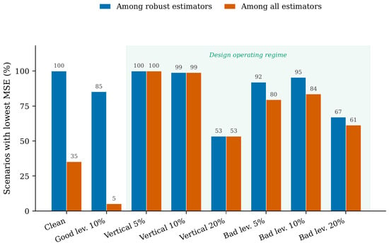
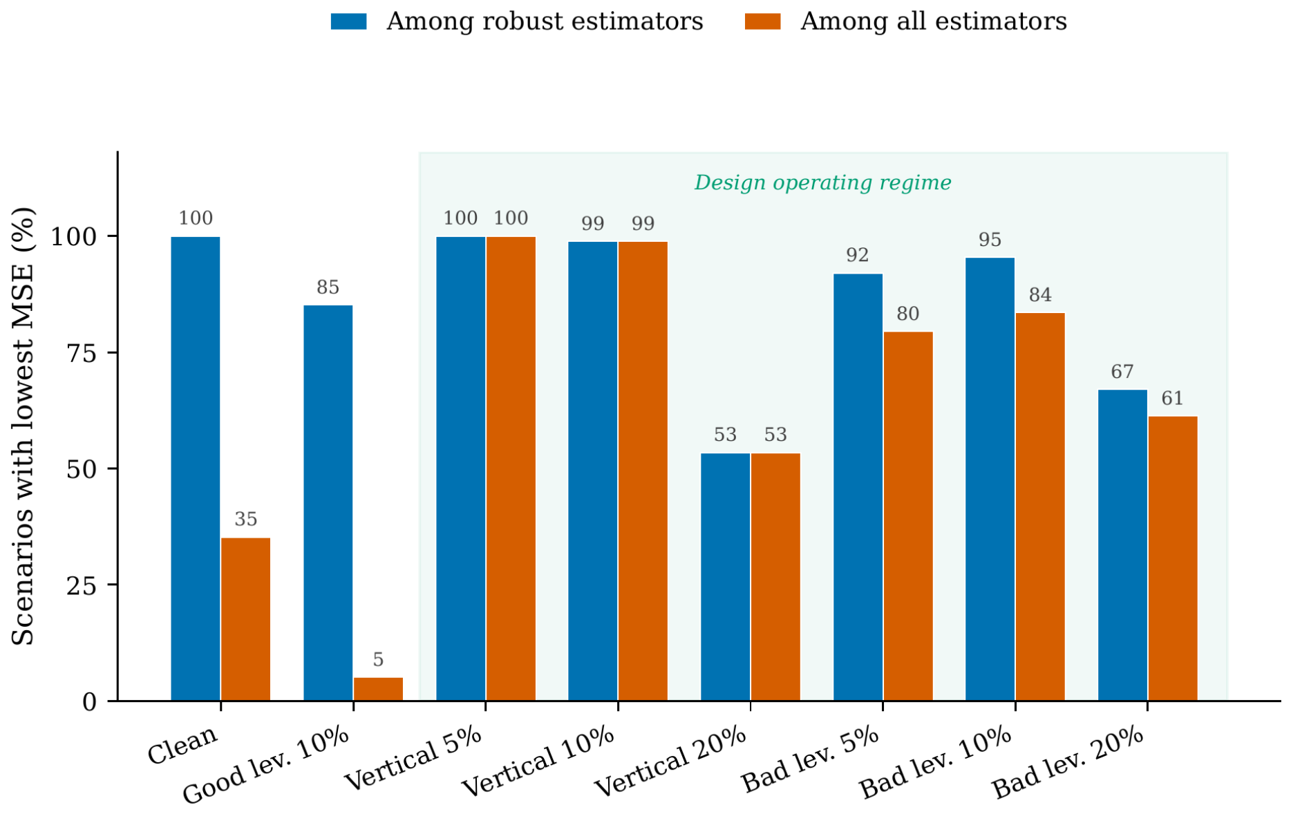
Figure 1 reports the percentage of simulation configurations in which ATLAS-Ridge attains the smallest mean squared error, by contamination type, both among the robust estimators and among the full set of eleven estimators. The corresponding median mean squared errors and median ratios to the best competing estimator are reported in Table 6.

Figure 1. Percentage of simulation configurations in which ATLAS-Ridge attains the smallest mean squared error, by contamination type, among the robust estimators and among all eleven.

Table 6. Mean squared error of ATLAS-Ridge relative to the competing estimators, by contamination type.

Contamination	Cfg.	Median MSE	Lowest (%)	Median Ratio
Clean	176	0.178	35.2	1.263
Good leverage 10%	176	0.253	5.1	2.800
Vertical 5%	176	0.175	100.0	0.650
Vertical 10%	176	0.183	98.9	0.729
Vertical 20%	176	0.220	53.4	0.964
Bad leverage 5%	176	0.220	79.5	0.792
Bad leverage 10%	176	0.217	83.5	0.815
Bad leverage 20%	176	0.252	61.4	0.911

Note. Median mean squared error of ATLAS-Ridge relative to the best competing estimator. Percentages are against all eleven.

Across the 1056 contaminated configurations, ATLAS-Ridge attains the smallest mean squared error in 79.5% of cases among all estimators and in 84.5% among the robust estimators, with a median performance ratio of 0.791 relative to the best competitor. The advantage is largest under vertical contamination, where the proposed estimator attains the smallest median mean squared error in $100.0\%$ of configurations at the $5\%$ level and $98.9\%$ at the $10\%$ level. The figure falls as the contamination level rises, to $53.4\%$ under $20\%$ vertical contamination and $61.4\%$ under $20\%$ bad leverage, reflecting the increasing difficulty of estimation near the breakdown region. In contrast, under 10% good-leverage contamination, the win rate among all estimators was 5.1%, indicating that when leverage observations remain consistent with the underlying regression model, conventional non-robust estimators may retain superior efficiency. This behavior is consistent with the theoretical properties established in Proposition 1.

Good leverage is the setting in which the estimator performs least favorably. The median ratio in Table 6 is $2.800$ there, almost three times the best competitor, against $0.650$ to $0.964$ under genuine contamination. Table 4 locates it: ridge with a generalized cross-validation constant attains $0.081$ against $0.253$ for ATLAS-Ridge. The winner is not a robust estimator; among the seven robust competitors, the proposal still has the smallest median, $0.253$ against $0.363$. The deficit is therefore against lightly penalized least squares, which is as expected: when no observation departs from the model, attenuating high-leverage points discards the most informative ones for nothing in return. This loss is intrinsic to the design, and the estimator should not be used where leverage points are believed sound.

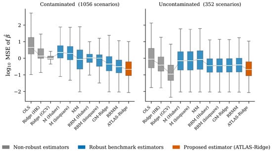
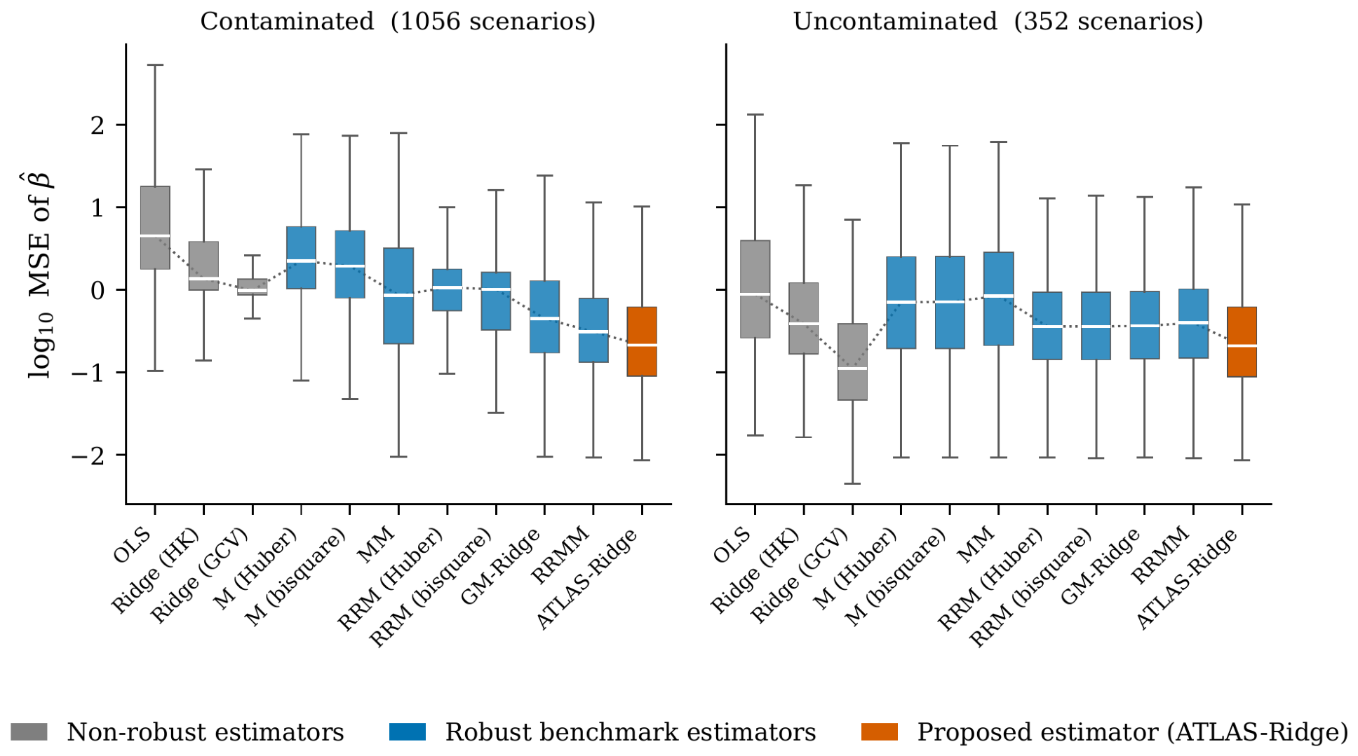
Figure 2 compares the distribution of ${\log }_{10}MSE$ for all estimators, under contaminated and uncontaminated configurations, while Table 7 summarizes their median mean squared error and mean rank. Under contaminated configurations, ATLAS-Ridge achieves the lowest median mean squared error (0.213) and the best overall mean rank (1.25), compared with 0.310 and 2.29, respectively, for the strongest competing estimator. These results indicate that the proposed method provides consistently superior estimation accuracy across a wide range of contaminated scenarios. The criterion throughout this section is the estimation error $\parallel \widehat{\beta }{-\beta \parallel }_2^2$ of Section 5.1. No predictive criterion is evaluated in the simulation study, and the conclusions drawn here therefore concern the recovery of $\beta$ and not out-of-sample prediction, which is examined separately in Section 6.

Figure 2. Distribution of the mean squared error of each estimator across the simulation configurations.

Table 7. Mean squared error and mean rank of each estimator over the simulation configurations.

Estimator	Median MSE		Ratio to	Mean Rank
	Contam.	All	ATLAS-Ridge
OLS	4.520	3.538	21.22	10.19
Ridge (HK)	1.353	1.147	6.35	7.81
Ridge (GCV)	0.979	0.954	4.60	5.79
M (Huber)	2.245	1.774	10.54	9.15
M (bisquare)	1.944	1.618	9.13	8.30
$MM$	0.863	0.856	4.05	6.22
RRM (Huber)	1.064	0.998	5.00	5.96
RRM (bisquare)	1.014	0.962	4.76	5.07
RRMM	0.310	0.328	1.46	2.29
GM-Ridge	0.447	0.411	2.10	3.97
ATLAS-Ridge	0.213	0.212	1.00	1.25

Note. Ratios and ranks refer to contaminated configurations.

Table 4 reports the median mean squared error of each estimator across the levels of the simulation factors. The first panel summarizes results by contamination type over all configurations, while the remaining five panels report results by sample size, number of predictors, collinearity level, error distribution, and error variance over the contaminated configurations.

Four observations emerge from Table 4. First, the ranking of the estimators is stable across levels of every factor: across contaminated configurations, ATLAS-Ridge attains the smallest median mean squared error at every sample size, dimension, collinearity level, error distribution, and error variance. Second, under uncontaminated conditions, shown in the first two rows of the first panel of Table 4, ridge regression with a generalized cross-validation constant attains the smallest median mean squared error. This is the expected outcome when no observation departs from the model, and it is consistent with the boundedness property established in Proposition 1. Third, the proposed estimator improves on the best plug-in robust ridge estimator at every error law, by a factor ranging from $1.15$ under $t_5$ errors to $1.68$ under $t_3$, with no monotone relation to tail weight. Fourth, the median mean squared error increases with collinearity and, subject to the qualification below, with error variance, consistently across the estimators. It does not decline monotonically with the sample size. For all eleven estimators the median is higher at $n=100$ than at $n=50$, before declining at $n=200$ and $n=500$. This is an artifact of the aggregation rather than a property of the estimators. The next paragraph gives the reason.

The cause is that the design of Section 5.1 is the union of two arms rather than a full factorial. One arm varies the error law over all six and the error variance over ${\sigma }^2\in \{1,5,10\}$, but only at the reference configuration $(n,p)=(100,8)$; the other varies n, p, and $\rho$ with ${\sigma }^2=1$ and only the normal and $t_3$ laws. The first arm lies entirely at $n=100$. Of the 576 contaminated configurations there, half have ${\sigma }^2\in \{5,10\}$, whereas all 96 at $n=50$ and all 192 at each of $n=200$ and $n=500$ have ${\sigma }^2=1$. Since the mean squared error scales with ${\sigma }^2$, the median at $n=100$ is raised by the composition of its set. The restriction $n\ge 5p$ adds a second imbalance, leaving only $p\in \{4,8\}$ at $n=50$. Two of the six panels are balanced: contamination, at 176 configurations per level, and collinearity, at 264, both with identical composition across levels. The other four are not, because the extra error laws and variances occur only at $(n,p)=(100,8)$.

What every panel does support, balanced or not, is comparison between estimators within a row, since all eleven are evaluated on the same configurations at each level. The four observations above are of that kind, and so is the first claim in this section. Comparison down a column is reliable only in the contamination and collinearity panels. The aggregate statements that do not depend on the balance of any panel are those of Figure 2 and Table 7, where the estimators are compared on the whole contaminated set at once.

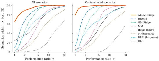
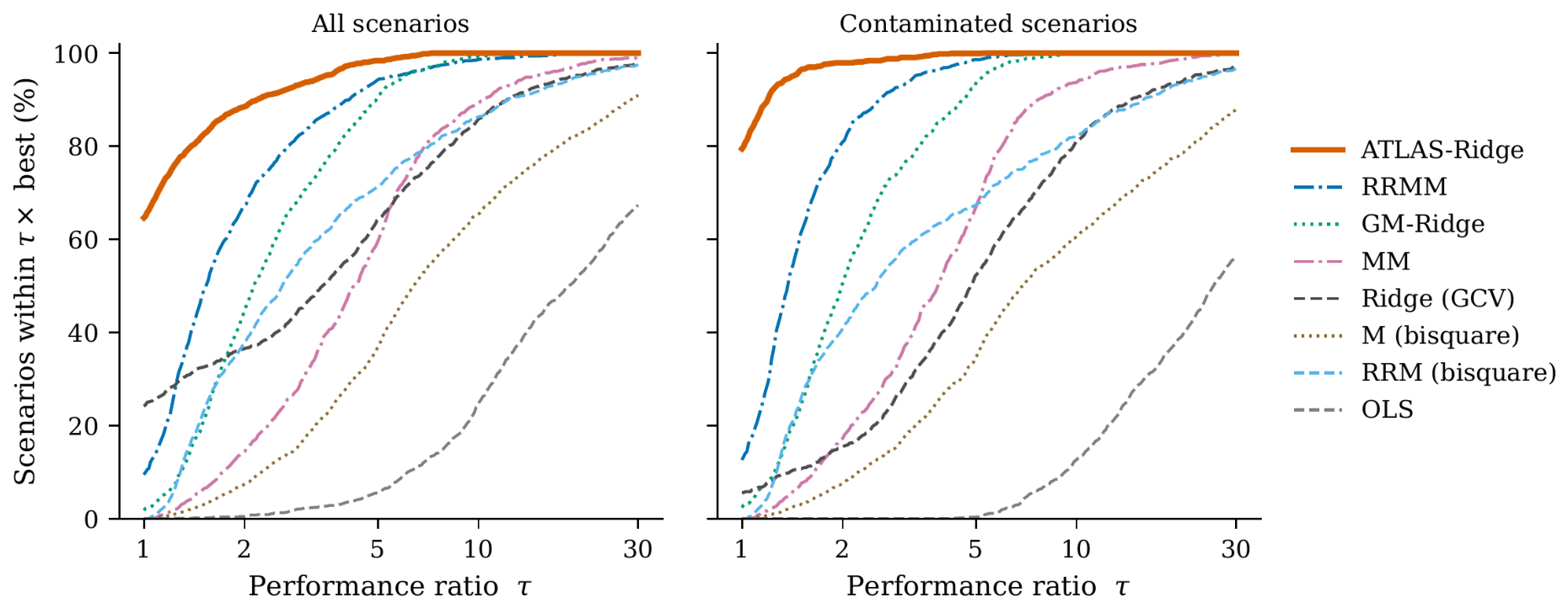
Figure 3 presents performance profiles [62], which report the fraction of configurations in which an estimator is within a factor $\tau$ of the best estimator. ATLAS-Ridge is within a factor of two of the best estimator in more than 90% of contaminated configurations, a level reached by no competing estimator below $\tau =4$.

Figure 3. Performance profiles of the estimators over the simulation configurations.

6. Application to Real Data

6.1. Entry Criteria and Data Sources

Datasets were selected using the following criteria: continuous predictors and response; $n\ge 8p$; a condition number of at least 30 or at least two variance inflation factors exceeding ten; at least four bad-leverage observations identified jointly in the design and residual spaces; and a total flagged fraction below the 25% breakdown point of the robust scatter estimator. An absolute count is used rather than a proportion because contamination in curated datasets is low, the largest bad-leverage fraction among the three observational datasets being $3.4\%$.

The Air Quality data [63] contain hourly measurements from a gas multisensor device, with carbon monoxide concentration as the response; cross-sensitivity among the sensors induces substantial multicollinearity. The Concrete Compressive Strength data [64] relate compressive strength to mixture composition and curing age. The Boston Housing data [65] relate median home value in 506 census tracts to nine predictors. The first two are obtained from the UCI Machine Learning Repository [66], and the third is distributed with the MASS package [61]. The Hawkins, Bradu, and Kass data [57] are a constructed benchmark that includes a planted bad-leverage cluster.

The Boston Housing data deviate from the criteria in that the flagged fraction is 31.6% and the bad-leverage fraction 3.4%. The excess arises from the good-leverage class, since three predictors are recorded at the town rather than the census-tract level [67], so the resulting high-leverage observations reflect measurement resolution rather than contamination. The data are retained because they contain 17 bad-leverage observations in ten distinct clusters.

Observations are classified as regular, vertical outliers, good leverage, or bad leverage using the robust distance in Equation (10) and standardized $MM$ residuals, against the thresholds ${\chi }_{p,0.975}^2$ and 2.5 [68]. Table 8 reports the resulting diagnostics.

Table 8. Characteristics of the datasets used in the application study.

Characteristic	Air Quality	Concrete	Boston	HBK
Observations n	3500	1030	506	75
Predictors p	10	8	9	3
Condition number	261.3	75.9	30.3	154.2
VIFs exceeding ten	4	0	0	3
Regular	2687	853	346	61
Vertical outliers	130	8	9	0
Good leverage	577	150	134	10
Bad leverage	106	19	17	4
Flagged fraction (%)	23.2	17.2	31.6	18.7

Note. The air quality data were analyzed on a random subsample.

6.2. Evaluation Criteria

Since $\beta$ is unknown for real data, the mean squared error of $\widehat{\beta }$ cannot be evaluated. Three computable criteria are therefore used. The first is the change in the coefficient vector when the observations classified as bad leverage are deleted,

$$\mathsf{\Delta }=100\times ∥{\widehat{\beta }}_{\mathrm{full}}-{\widehat{\beta }}_{\mathrm{deleted}}∥/∥{\widehat{\beta }}_{\mathrm{deleted}}^{MM}∥,$$

(22)

which is a finite-sample diagnostic motivated by the property bounded in Proposition 1, computed both with the tuning held at its full-sample values and with the tuning determined on the reduced sample. The denominator is the norm of the $MM$ fit on the reduced sample and is the same for every estimator, so that displacements are comparable across estimators; normalizing each by its own coefficient norm would favor an estimator that shrinks more. The two regimes correspond to the distinction drawn in Section 4.4. Holding the tuning fixed corresponds to the regime of the conditional bound of Proposition 1, in which the tuning quantities are held fixed; determining the tuning on the reduced sample measures the displacement of the fully adaptive estimator, for which no influence function is derived. The gap between the two is therefore an empirical measure of how much the adaptive tuning contributes to the coefficient displacement. The second is the ten-fold cross-validated prediction error with 10% symmetric trimming. The third comprises the bootstrap variance $\mathrm{tr}\left(\widehat{\mathrm{Var}}\right)/{\parallel \widehat{\beta }\parallel }^2$ and the split-half stability $\parallel {\widehat{\beta }}_1-{\widehat{\beta }}_2\parallel /\parallel \widehat{\beta }\parallel$, based on 200 resamples and 100 random half-splits.

These criteria measure two different things and are not expected to be optimized together. The displacement of Equation (22), the bootstrap variance, and the split-half stability all concern the coefficient vector; the cross-validated prediction error concerns the fitted response and is evaluated on the observed data, contamination included. An estimator that downweights high-leverage observations forfeits the fit at the points contributing most to the predictive sum of squares, so a gain on the first group is bought at a cost on the second. The two groups are therefore reported separately rather than combined into one ranking. Note also that Equation (16) minimizes a reference-weighted estimate of prediction risk, with outliers and high-leverage points downweighted, while the error reported here is computed over the full sample; selecting $\widehat{k}$ by a predictive criterion therefore implies nothing about unweighted prediction error.

6.3. Results and Discussion

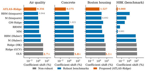
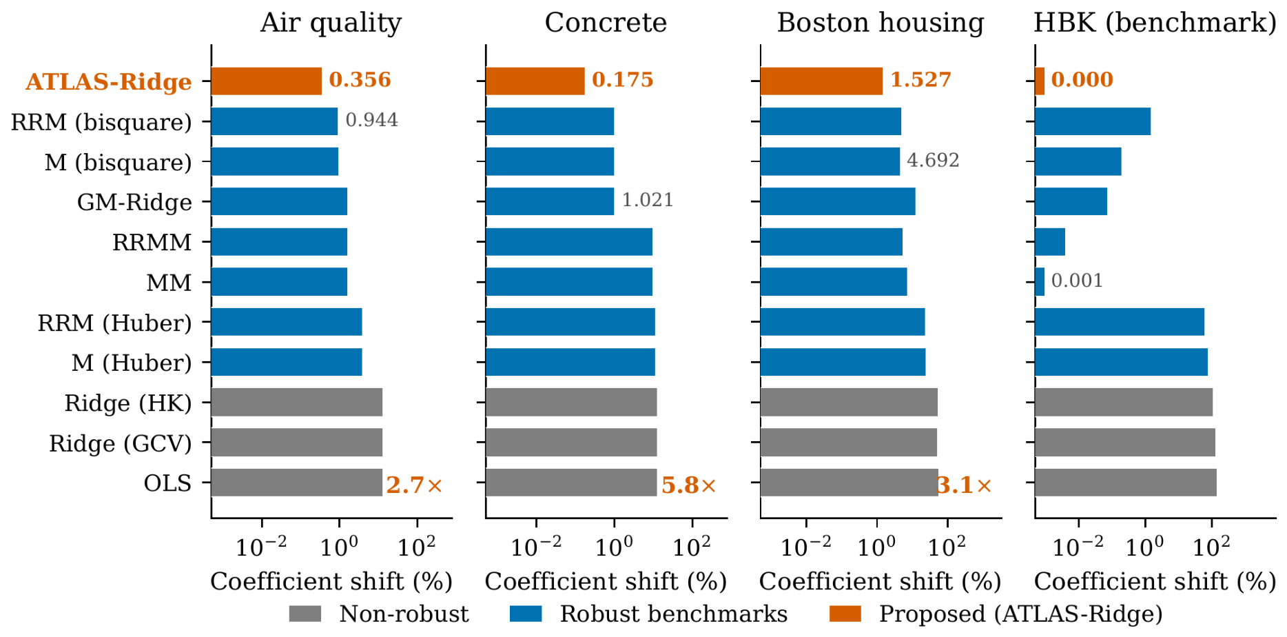
Figure 4 compares the estimators in terms of the quantity defined in Equation (22), namely the change in the estimated coefficient vector when the bad-leverage observations are deleted, expressed as a percentage of the coefficient norm. A small value indicates that an estimator is little affected by those observations. ATLAS-Ridge attains the smallest value on all four datasets. Each comparison below is made against the estimator that attains the second smallest value on that dataset. On the air quality data, the coefficients of ATLAS-Ridge change by $0.487\%$, against $1.628\%$ for the robust ridge M-estimator with bisquare loss. On the concrete data they change by $0.175\%$, against $0.667\%$ for the Mallows-type generalized M ridge estimator. On the Boston data, the change is below $0.001\%$, against $2.341\%$ for the same estimator. The corresponding reductions are by factors of $3.3$, $3.8$, and more than two orders of magnitude. On the benchmark the change is 0.000%, since the planted observations receive zero weight, whereas the coefficients of OLS change by 142% and one of them reverses sign.

Figure 4. Relative change in the estimated coefficients after deletion of the bad-leverage observations, by estimator and dataset.

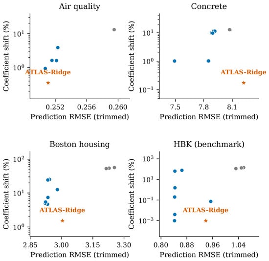
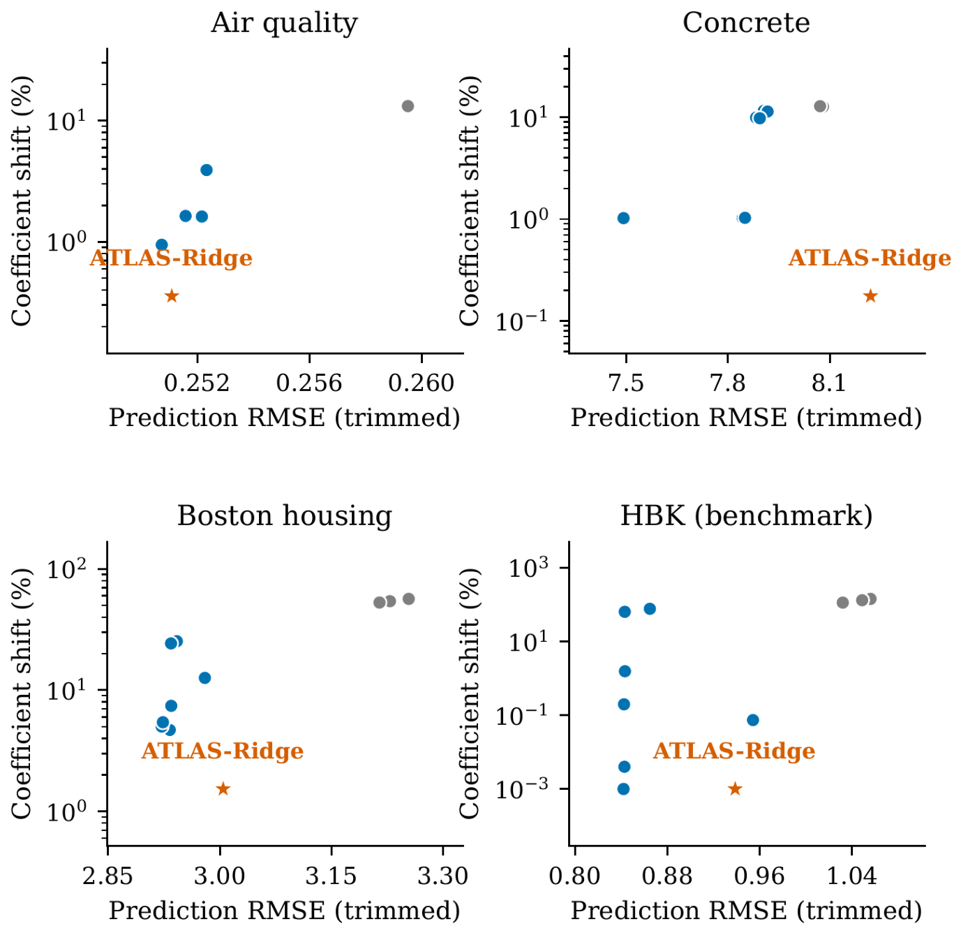
Table 9 summarizes the performance of the eleven estimators across the four evaluation criteria and datasets. ATLAS-Ridge achieves the smallest coefficient displacement across all four datasets when the tuning is held at its full-sample value, while its rankings for prediction error, bootstrap variance, and split-half stability vary by dataset. The prediction ranking varies most, and it does not favor the proposed estimator. On the air quality data, it ties for first with two bisquare M-estimators at $0.251$; on HBK and Boston it places seventh and eighth of eleven, exceeding the best competitor by $11.5\%$ and $2.8\%$; and on the concrete data it places last, at $8.220$ against $7.492$ for GM-Ridge, a shortfall of $9.7\%$. Across the four datasets, it matches the best competitor on one and records higher prediction error on the other three. The shortfall does not track contamination: it is largest on HBK and concrete, at flagged fractions of $18.7\%$ and $17.2\%$, and smallest, among the three datasets on which one arises at all, on Boston, whose flagged fraction is the largest at $31.6\%$. It reflects instead the mechanism noted with Figure 5, that design-direction attenuation acts on all high-leverage observations, not only the harmful ones. The variability of those rankings is consistent with Remark 1 of Section 4.4, since the adaptive tuning estimates several quantities from the data and is therefore more variable with moderate sample sizes.

Table 9. Coefficient robustness and predictive accuracy of each estimator on the four real datasets.

Estimator	Displacement (%)				Prediction Error				Bootstrap Variance ($\times {10}^{-3}$)				Split-Half Stability (%)
	Air				Air				Air				Air
	Quality	Concrete	Boston	HBK	Quality	Concrete	Boston	HBK	Quality	Concrete	Boston	HBK	Quality	Concrete	Boston	HBK
OLS	13.23	12.92	56.53	142.3	0.260	8.066	3.254	1.056	10.6	18.2	42.2	514	20.7	22.0	45.9	128.2
Ridge (HK)	13.15	12.71	54.11	112.4	0.259	8.079	3.229	1.032	10.3	18.9	45.9	648	20.2	22.1	40.3	136.6
Ridge (GCV)	13.21	12.87	52.70	130.8	0.260	8.071	3.215	1.049	10.5	19.5	40.8	630	20.6	23.0	38.9	134.6
M (Huber)	3.93	11.56	25.28	76.5	0.252	7.905	2.942	0.865	4.3	17.1	42.0	513	13.2	22.1	41.2	127.4
M (bisquare)	0.95	1.02	4.69	0.198	0.251	7.843	2.933	0.842	4.5	30.4	35.2	871	12.7	29.7	36.8	113.7
$MM$	1.64	9.94	7.42	0.001	0.252	7.882	2.935	0.842	4.3	21.8	36.1	239	12.6	24.5	38.2	82.9
RRM (Huber)	3.92	11.39	24.23	63.6	0.252	7.916	2.934	0.843	4.3	17.8	40.8	656	13.0	22.4	38.0	137.3
RRM (bisquare)	0.94	1.03	5.00	1.550	0.251	7.850	2.922	0.843	4.4	30.9	28.4	899	12.5	29.7	32.4	93.7
RRMM	1.64	9.79	5.42	0.004	0.252	7.893	2.924	0.843	4.3	22.6	34.8	176	12.5	24.6	35.1	60.6
GM-Ridge	1.62	1.02	12.61	0.074	0.252	7.492	2.980	0.954	3.6	9.2	30.8	146	11.9	17.0	31.6	57.1
ATLAS-Ridge	0.36	0.18	1.53	0.000	0.251	8.220	3.005	0.939	3.8	24.7	15.5	230	12.2	25.5	22.8	84.1

Note. Displacement, bootstrap variance and split-half stability measure coefficient robustness; the prediction error measures predictive accuracy. Displacement is defined in Equation (22); the prediction error is the ten-fold cross-validated trimmed root mean squared error. Bold marks the columns in which ATLAS-Ridge attains the smallest value.

Figure 5. Relative change in the estimated coefficients after deletion of the bad-leverage observations against cross-validated prediction error, by estimator and dataset.

The Boston Housing data provide the strongest evidence for the estimator, which attains the best performance on three of the four criteria: coefficient displacement below $0.001\%$ against $2.341\%$, normalized bootstrap variance $15.5\times {10}^{-3}$ against $28.4\times {10}^{-3}$, and split-half stability 22.8% against 31.6%, while its prediction error exceeds that of the best competitor by 2.8%. The selected shrinkage constant is $\widehat{k}=18.33$, so the penalty acts on the poorly determined directions while leaving the leading ones essentially unshrunk, and the observed stability reflects the adaptive loss and the penalty together.

Figure 5 displays the coefficient displacement and prediction error jointly. ATLAS-Ridge occupies the lower region of every panel, while its prediction error varies across datasets. Bounded influence in the design direction requires the attenuation of all high-leverage observations, including informative ones; since these outnumber bad-leverage observations by between two and a half and eight to one, the loss in predictive efficiency is incurred more broadly than the robustness benefit is realized.

Table 10 reports the tuning selected for each dataset and the change in the coefficients when the tuning is determined on the reduced sample rather than on the full sample. Table 11 gives both quantities for all eleven estimators on all four datasets, with the tuning of every estimator held at its full-sample value in one column and determined on the reduced sample in the other, so that the two regimes are compared on the same footing. The estimated tail index ranges from 3.01 to 4.40 and the shrinkage constant $\widehat{k}$ from 0 to 127.4, so the procedure adapts to each dataset. Determining the tuning on the reduced sample increases the displacement for the air quality and concrete data, most markedly for the latter, where it rises from 0.175% to 11.558%.

Table 10. Selected tuning constants and coefficient displacement under full-sample and reduced-sample tuning.

Quantity	Air Quality	Concrete	Boston	HBK
Tail index $\widehat{\alpha }$	3.31	4.25	2.88	4.40
Shape $\widehat{q}$	2.19	2.59	2.00	2.64
Scale ${\widehat{c}}_0$	2.29	2.39	2.23	2.40
Implied $\alpha =2/{\widehat{c}}_0^2$	–	–	0.402	–
Shrinkage $\widehat{k}$	4.281	127.4	18.33	0.000
Displacement, full-sample tuning (%)	0.487	0.175	0.000	0.000
Displacement, reduced-sample tuning (%)	0.737	11.558	7.434	0.001

Note. Displacement is defined in Equation (22). The implied constant is reported only where $\widehat{q}$ is close to 2.

Table 11. Coefficient displacement of each estimator under full-sample and reduced-sample tuning, by dataset. Displacement is defined in Equation (22).

	Air Quality		Concrete		Boston		HBK
Estimator	Full	Reduced	Full	Reduced	Full	Reduced	Full	Reduced
OLS	21.44	21.44	12.92	12.92	58.14	58.14	142.25	142.25
Ridge (HK)	20.90	21.18	12.80	12.71	54.77	55.33	116.29	112.45
Ridge (GCV)	20.71	21.51	12.87	12.87	54.00	54.00	122.61	130.82
M (Huber)	6.07	8.48	7.36	11.56	18.95	26.54	74.02	76.53
M (bisquare)	1.66	2.12	0.70	1.02	3.59	5.41	0.00	0.20
$MM$	2.87	3.66	5.70	9.94	6.39	8.95	0.00	0.00
RRM (Huber)	6.00	8.42	7.31	11.39	18.04	25.52	60.04	63.63
RRM (bisquare)	1.63	2.12	0.70	1.03	3.41	5.26	0.00	1.55
RRMM	2.82	3.65	5.65	9.79	6.05	8.70	0.00	0.00
GM-Ridge	2.19	3.49	0.67	1.02	2.34	28.24	0.00	0.07
ATLAS-Ridge	0.49	0.74	0.18	11.56	0.00	7.43	0.00	0.00

Note. Full denotes the tuning of every estimator held at its full-sample value; Reduced denotes the tuning of every estimator determined by its own rules on the reduced sample. Values are percentages. The smallest value in each column is in bold. On the concrete data, the absolute movement of ATLAS-Ridge is $2.359$ against $0.208$ for GM-Ridge, on a coefficient norm of $13.21$ against $21.65$.

That sixty-six-fold increase is the largest instability in the application study. Two observations bear on it, neither conclusive. The concrete fit is the only one with a materially active penalty, $\widehat{k}=127.4$ against $2.637$ and $0.000$; and the absolute movement of its coefficient vector, $2.359$ on the standardized scale, is of the same size as that of the M- and $MM$-based estimators, whose displacements are similar once the common normalizer is applied. Whether the first is causal is not established: a simulated experiment varying $\widehat{k}$ through the collinearity level found no positive association between its size and the increase under reduced-sample tuning, the rank correlation being negative. The result is therefore reported as an instability whose mechanism is not identified. That experiment did show re-selection to be common, the search on the reduced sample returning a different constant in half of the replications, which locates the instability in the selection step.

Two qualifications follow. The displacement under full-sample tuning, $0.175\%$, is a finite-deletion diagnostic computed in the regime to which Proposition 1 applies, the tuning quantities being held fixed. The proposition bounds infinitesimal influence and does not bound this finite percentage, so the figure is empirical evidence consistent with bounded influence rather than an instance of the bound. It remains the smallest among the eleven estimators on this dataset; the figure under reduced-sample tuning measures something the theory does not cover, namely the composite functional in which the scale, the scatter, the loss parameters, and the shrinkage constant are all determined from the data. The gap between the two is the empirical cost of adaptivity, and on the concrete data that cost is high. Since the procedure is presented as adaptive, this is a limitation of the proposal and not an artifact of the displacement measure: a user who determines the whole pipeline anew after removing suspect observations should allow for the coefficients moving appreciably, and the present evidence does not identify in advance the datasets on which that will happen. Stabilizing the selection of k under resampling, for instance by averaging the criterion over subsamples rather than minimizing it once, is the natural remedy and is not attempted here.

The Boston fit gives a direct check on the correspondence of Section 3.1. There $\widehat{q}=2.00$, so the loss coincides with the Welsch score and the implied density power divergence constant is $\alpha =2/{\widehat{c}}_0^2=0.402$. Substituting that value into the asymptotic efficiency expression of Riani et al. [44] returns $0.879$, against the target $0.879$ set by Equation (8) at $\widehat{\alpha }=2.88$. The calibration of Equation (7) therefore reproduces, on real data, the efficiency that those authors tabulate for the fixed-tuning density power divergence estimator, which locates the fitted loss inside an established family. The air quality, concrete, and HBK fits select $\widehat{q}=2.19$, $2.59$, and $2.64$ and so fall outside it; for these the shape itself, rather than the scale alone, carries the adaptation.

One entry of Table 10 requires comment. The shrinkage selected on the HBK data is reported as $\widehat{k}=0.000$, which is the smallest value the grid admits at the reported precision. Proposition 2 is stated for $k>0$ and for a selected $\widehat{k}$ lying in $\mathcal{K}\setminus \left\{0\right\}$, so if the criterion has in fact chosen the unpenalized member of the grid on this dataset, the breakdown statement does not cover that particular fit; the bound of Equation (18), which also requires $k>0$, likewise does not. The displacement of $0.000\%$ recorded for HBK is therefore an empirical observation about the leverage-weighted M-fit on these data and is not an instance of the proposition. The planted observations in this dataset lie far enough from the bulk in the design space that the attenuation of Section 3.4 reduces their weights to numerical zero, which accounts for the result without appeal to the penalty.

The evidence supports a specific rather than a universal claim. Under simultaneous contamination and severe multicollinearity, ATLAS-Ridge attains the smallest mean squared error in most simulated configurations and the smallest coefficient displacement on every real dataset under full-sample tuning. Two qualifications belong with that claim. Good leverage is the one simulated setting in which it is reversed, and determining the whole pipeline anew rather than holding the tuning fixed raises the displacement on the concrete data by a factor of sixty-six, so the stability of the estimator is established for the conditional quantity of Proposition 1 and not for the adaptive procedure taken as a whole. In cross-validated prediction error, it matches the best competitor on one dataset and records higher error on the other three, and on one of the four it is the least accurate predictor of the eleven estimators compared. The two findings concern different quantities and both are retained here: the estimator is recommended where the coefficients are the object of inference, and it is not recommended where out-of-sample prediction is the objective, for which the bisquare M-estimators and GM-Ridge are preferable on these datasets. Its advantage therefore lies in estimation robustness rather than in uniformly superior prediction.

Three limitations should be acknowledged. First, bounded influence in the design direction necessarily attenuates all high-leverage observations, including informative ones, so the resulting loss of predictive efficiency is intrinsic to the estimator rather than a consequence of implementation. The simulation study quantifies this trade-off. Under $10\%$ good-leverage contamination, the proposed estimator has the smallest mean squared error in only $5.1\%$ of configurations and a median ratio of $2.800$ to the best competitor, both the worst values it records anywhere in the study. Good leverage is the one setting in which the design is deliberately informative and nothing is wrong with the data, and it is precisely there that attenuation costs most. Second, the adaptive tuning introduces finite-sample variability, since the loss parameters and the shrinkage constant are estimated from the data, and this variability can affect stability in moderate samples. The asymptotic results cover part of it: the bounded grid makes the penalty contribution negligible in Theorem 1, and Theorem 2 concerns the loss parameters under the symmetry conditions of Assumption 1. Neither establishes that estimating the scale and the scatter has no first-order effect. The boundedness result of Proposition 1 is likewise conditional on the tuning, and the influence function of the composite functional, in which the scale, the scatter, the loss parameters, and the shrinkage constant are all estimated, is not derived here. Third, the real-data evaluation is constrained by the low prevalence of bad-leverage observations in observational data, so the applications illustrate robustness under mild contamination but provide no evidence at the more severe levels examined in the simulation study. It is also constrained in design. Stability is assessed by deleting the observations that the diagnostics of Section 6.1 classify as bad leverage, and those diagnostics use the same robust distance and the same MM residuals that the estimator itself uses. An estimator built on a given notion of outlyingness will tend to look stable when judged against that notion. Evidence from a perturbation scheme that does not share the diagnostic, such as random case resampling, coordinatewise contamination of a fixed fraction of cells [69,70], or small displacements applied to observations the diagnostics regard as regular, would be complementary and is not reported here. The advantage reported in Section 5 is also specific to the orientation of the coefficient vector used there: with the signal on the smallest eigenvector or spread equally over the eigendirections, the Mallows-type generalized M ridge estimator attains the smaller median mean squared error in every contamination scheme, as Section S8 of the Supplementary Materials reports. The comparison under reduced-sample tuning in Table 10 does not escape this dependence: the same diagnostics determine which observations are deleted, and reduced-sample tuning changes the treatment of the tuning rather than the selection of the deleted cases. The concrete result in that table is the reason the issue is raised.

7. Conclusions

This paper proposed ATLAS-Ridge, a penalized generalized M-estimator for linear regression under multicollinearity and data contamination. The method combines an adaptive redescending loss function, robust-distance-based observation weights, and ridge parameter selection through a reference-weighted generalized cross-validation criterion. Simulation studies and real-data applications demonstrate competitive estimation performance and improved coefficient stability under bad-leverage contamination when tuning parameters are fixed at their full-sample values. However, this stability advantage weakens when the tuning is determined on the reduced sample, particularly for the concrete dataset. The estimator also performs least favorably under good-leverage contamination, while its predictive accuracy ranges from best to worst among the eleven methods considered. The simulation advantage is specific to the orientation of the coefficient vector adopted in the design and does not persist when the signal lies in the poorly identified directions. These findings highlight the trade-off between estimation robustness and predictive performance. Future research will focus on improving the finite-sample stability of adaptive tuning, extending the method to generalized linear models, and accommodating cellwise contamination.

References

- Iftikhar, H.; Shah, S.F.; Almuhayfith, F.E.; Canas, P. A Kernel Regression-Based Hybrid Forecasting Framework for Highly Volatile Energy Commodity Markets. Aims Math. 2026, 11, 24877–24912. [Google Scholar] [CrossRef] [Scilit]
- Iftikhar, H.; Shah, S.F.; Rodrigues, P.C.; Alamri, O.A.; Alsaedi, B.S.O. A Novel Kernel Regression-Based Decomposition Hybrid Framework for Forecasting Cryptocurrency Markets. IEEE Access 2026, 14, 133335–133360. [Google Scholar] [CrossRef] [Scilit]
- Iftikhar, H.; Shah, S.F.; Almuhayfith, F.E.; Rodrigues, P.C. A Flexible Kernel Regression Decomposition-Based Hybrid Framework for Forecasting Foreign Exchange Rates: Uncovering Symmetric and Asymmetric Market Dynamics. Symmetry 2026, 18, 1372. [Google Scholar] [CrossRef] [Scilit]
- Hoerl, A.E.; Kennard, R.W. Ridge regression: Biased estimation for nonorthogonal problems. Technometrics 1970, 12, 55–67. [Google Scholar] [CrossRef] [Scilit]
- Marquardt, D.W.; Snee, R.D. Ridge regression in practice. Am. Stat. 1975, 29, 3–20. [Google Scholar] [CrossRef] [Scilit]
- Shah, I.; Iftikhar, H.; Ali, S. Modeling and Forecasting Electricity Demand and Prices: A Comparison of Alternative Approaches. J. Math. 2022, 2022, 3581037. [Google Scholar] [CrossRef] [Scilit]
- Nawaz, S.; Haider, B.; Zaman, Q. Combine Solution to Multicollinearity and Outlier: A New Family of Estimators Based on old Robust Ridge M-Estimator. J. Multidiscip. Appl. Stat. Sci. 2026, 2, 01–22. [Google Scholar] [CrossRef]
- Huber, P.J. Robust estimation of a location parameter. Ann. Math. Stat. 1964, 35, 73–101. [Google Scholar] [CrossRef] [Scilit]
- Hampel, F.R. The influence curve and its role in robust estimation. J. Am. Stat. Assoc. 1974, 69, 383–393. [Google Scholar] [CrossRef] [Scilit]
- Hoerl, A.E.; Kennard, R.W.; Baldwin, K.F. Ridge regression: Some simulations. Commun. Stat. 1975, 4, 105–123. [Google Scholar] [CrossRef] [Scilit]
- McDonald, G.C.; Galarneau, D.I. A Monte Carlo evaluation of some ridge-type estimators. J. Am. Stat. Assoc. 1975, 70, 407–416. [Google Scholar] [CrossRef]
- Kibria, B.M.G. Performance of some new ridge regression estimators. Commun. Stat. Simul. Comput. 2003, 32, 419–435. [Google Scholar] [CrossRef] [Scilit]
- Golub, G.H.; Heath, M.; Wahba, G. Generalized cross-validation as a method for choosing a good ridge parameter. Technometrics 1979, 21, 215–223. [Google Scholar] [CrossRef] [Scilit]
- Norouzirad, M.; Arashi, M. Preliminary test and Stein-type shrinkage ridge estimators in robust regression. Stat. Pap. 2019, 60, 1849–1882. [Google Scholar] [CrossRef] [Scilit]
- Arashi, M.; Norouzirad, M.; Ahmed, S.E.; Yuzbasi, B. Rank-based Liu regression. Comput. Stat. 2018, 33, 1525–1561. [Google Scholar] [CrossRef] [Scilit]
- Liu, K. A new class of biased estimate in linear regression. Commun. Stat. Theory Methods 1993, 22, 393–402. [Google Scholar] [CrossRef] [Scilit]
- Wu, Y. Can’t Ridge Regression Perform Variable Selection? Technometrics 2021, 63, 263–271. [Google Scholar] [CrossRef] [Scilit]
- Chen, L.-P. Variable selection via penalized ridge regression with error-prone variables. Ann. Inst. Stat. Math. 2026, 78, 225–261. [Google Scholar] [CrossRef] [Scilit]
- Huber, P.J. Robust regression: Asymptotics, conjectures and Monte Carlo. Ann. Stat. 1973, 1, 799–821. [Google Scholar] [CrossRef] [Scilit]
- Beaton, A.E.; Tukey, J.W. The fitting of power series, meaning polynomials, illustrated on band-spectroscopic data. Technometrics 1974, 16, 147–185. [Google Scholar] [CrossRef] [Scilit]
- Holland, P.W.; Welsch, R.E. Robust regression using iteratively reweighted least-squares. Commun. Stat. Theory Methods 1977, 6, 813–827. [Google Scholar] [CrossRef] [Scilit]
- Rousseeuw, P.J. Least median of squares regression. J. Am. Stat. Assoc. 1984, 79, 871–880. [Google Scholar] [CrossRef]
- Rousseeuw, P.J.; Yohai, V.J. Robust regression by means of S-estimators. In Robust and Nonlinear Time Series Analysis; Lecture Notes in Statistics; Springer: New York, NY, USA, 1984; Volume 26, pp. 256–272. [Google Scholar]
- Yohai, V.J. High breakdown-point and high efficiency robust estimates for regression. Ann. Stat. 1987, 15, 642–656. [Google Scholar] [CrossRef] [Scilit]
- Simpson, D.G.; Ruppert, D.; Carroll, R.J. On one-step GM estimates and stability of inferences in linear regression. J. Am. Stat. Assoc. 1992, 87, 439–450. [Google Scholar] [CrossRef] [Scilit]
- Coakley, C.W.; Hettmansperger, T.P. A bounded influence, high breakdown, efficient regression estimator. J. Am. Stat. Assoc. 1993, 88, 872–880. [Google Scholar] [CrossRef]
- Koenker, R.; Bassett, G. Regression quantiles. Econometrica 1978, 46, 33–50. [Google Scholar] [CrossRef] [Scilit]
- Silvapulle, M.J. Robust ridge regression based on an M-estimator. Aust. J. Stat. 1991, 33, 319–333. [Google Scholar] [CrossRef] [Scilit]
- Askin, R.G.; Montgomery, D.C. Augmented robust estimators. Technometrics 1980, 22, 333–341. [Google Scholar] [CrossRef] [Scilit]
- Wasim, D.; Khan, S.A.; Suhail, M. Modified robust ridge M-estimators for linear regression models: An application to tobacco data. J. Stat. Comput. Simul. 2023, 93, 2703–2724. [Google Scholar] [CrossRef] [Scilit]
- Wasim, D.; Khan, S.A.; Suhail, M. Quantile-based robust ridge M-estimator for linear regression model in presence of multicollinearity and outliers. Commun. Stat. Simul. Comput. 2023, 52, 6134–6154. [Google Scholar]
- Wasim, D.; Khan, S.A.; Suhail, M. Quantile-based two-parameter robust ridge M-estimators for linear regression model. Statistics 2026. [Google Scholar] [CrossRef] [Scilit]
- Alharthi, M.F.; Akhtar, N. Newly improved two-parameter ridge estimators: A better approach for mitigating multicollinearity in regression analysis. Axioms 2025, 14, 186. [Google Scholar] [CrossRef] [Scilit]
- Akhtar, N.; Alharthi, M.F.; Khan, M.S. Mitigating multicollinearity in regression: A study on improved ridge estimators. Mathematics 2024, 12, 3027. [Google Scholar] [CrossRef] [Scilit]
- Ashraf, A.; Akhtar, N.; Alharthi, M.F. Robust Kibria estimators for mitigating multicollinearity and outliers in a linear regression model. Stats 2025, 8, 119. [Google Scholar] [CrossRef] [Scilit]
- Yasmin, N.; Kibria, B.M.G.; Bursac, Z. A Comparative Study of Robust and Improved Shrinkage Estimators Under Multicollinearity and Outliers Using Multiple Performance Criteria with Application to Health Data. Stats 2026, 9, 62. [Google Scholar] [CrossRef] [Scilit]
- Dawoud, I.; Abonazel, M.R.; Awwad, F.A. Robust-Stein estimator for overcoming outliers and multicollinearity. Sci. Rep. 2023, 13, 8949. [Google Scholar] [CrossRef] [Scilit] [PubMed]
- Suhail, M.; Khan, S.A.; Wasim, D. Bagging-based robust ridge M-estimators in linear regression model for mitigating multicollinearity and outliers. Commun. Stat. Theory Methods 2026. [Google Scholar] [CrossRef] [Scilit]
- Wasim, D.; Khan, S.A. Weighted robust improved KL M-estimators for linear regression model in presence of multicollinearity and outliers: Simulation and applications. Stat. Theory Relat. Fields 2026, 4, 2641776. [Google Scholar] [CrossRef] [Scilit]
- Abonazel, M.R.; Dawoud, I.; Awwad, F.A. New robust estimator for handling outliers and multicollinearity in gamma regression model with application to breast cancer data. Sci. Rep. 2025, 15, 38436. [Google Scholar] [CrossRef] [Scilit] [PubMed]
- Hammad, A.T.; Elbatal, I.; Almetwally, E.M.; Abd El-Raouf, M.M.; El-Qurashi, M.A.; Gemeay, A.M. A novel robust estimator for addressing multicollinearity and outliers in Beta regression: Simulation and application. AIMS Math. 2025, 10, 21549–21580. [Google Scholar] [CrossRef] [Scilit]
- Lukman, A.F.; Kibria, B.M.G.; Ayinde, K. Robust ridge estimators for handling multicollinearity and outliers in linear regression. Concurr. Comput. Pract. Exp. 2024, 36, e7975. [Google Scholar] [CrossRef] [Scilit]
- Basu, A.; Harris, I.R.; Hjort, N.L.; Jones, M.C. Robust and efficient estimation by minimising a density power divergence. Biometrika 1998, 85, 549–559. [Google Scholar] [CrossRef] [Scilit]
- Riani, M.; Atkinson, A.C.; Corbellini, A.; Perrotta, D. Robust regression with density power divergence: Theory, comparisons, and data analysis. Entropy 2020, 22, 399. [Google Scholar] [CrossRef] [Scilit] [PubMed]
- Sun, Q.; Zhou, W.-X.; Fan, J. Adaptive Huber regression. J. Am. Stat. Assoc. 2020, 115, 254–265. [Google Scholar] [CrossRef] [Scilit] [PubMed]
- Khan, S.A.; Wasim, D.; Suhail, M. Mitigating multicollinearity and outliers in regression: Comparison of some new and old robust ridge M-estimators. J. Stat. Comput. Simul. 2025, 95, 3526–3547. [Google Scholar] [CrossRef] [Scilit]
- Belsley, D.A.; Kuh, E.; Welsch, R.E. Diagnostics for collinearity. J. Am. Stat. Assoc. 1980, 75, 753–754. [Google Scholar]
- Jin, Y.; Olive, D.J. Large Sample Theory for Some Ridge-Type Regression Estimators. Stats 2026, 9, 65. [Google Scholar] [CrossRef] [Scilit]
- Dennis, J.E.; Welsch, R.E. Techniques for nonlinear least squares and robust regression. Commun. Stat. Simul. Comput. 1978, 7, 345–359. [Google Scholar] [CrossRef] [Scilit]
- Hill, B.M. A simple general approach to inference about the tail of a distribution. Ann. Stat. 1975, 3, 1163–1174. [Google Scholar] [CrossRef] [Scilit]
- Rousseeuw, P.J.; Van Driessen, K. A fast algorithm for the minimum covariance determinant estimator. Technometrics 1999, 41, 212–223. [Google Scholar] [CrossRef]
- Hubert, M.; Rousseeuw, P.J.; Verdonck, T. A deterministic algorithm for robust location and scatter. J. Comput. Graph. Stat. 2012, 21, 618–637. [Google Scholar] [CrossRef] [Scilit]
- Salibian-Barrera, M.; Yohai, V.J. A fast algorithm for S-regression estimates. J. Comput. Graph. Stat. 2006, 15, 414–427. [Google Scholar] [CrossRef] [Scilit]
- Maronna, R.A.; Yohai, V.J. Robust regression with both continuous and categorical predictors. J. Stat. Plan. Inference 2000, 89, 197–214. [Google Scholar] [CrossRef] [Scilit]
- Croux, C.; Dhaene, G.; Hoorelbeke, D. Robust Standard Errors for Robust Estimators; Discussion Paper Series DPS 03.16; Katholieke Universiteit Leuven: Leuven, Belgium, 2003. [Google Scholar]
- Craven, P.; Wahba, G. Smoothing noisy data with spline functions. Numer. Math. 1979, 31, 377–403. [Google Scholar] [CrossRef] [Scilit]
- Hawkins, D.M.; Bradu, D.; Kass, G.V. Location of several outliers in multiple regression data using elemental sets. Technometrics 1984, 26, 197–208. [Google Scholar] [CrossRef]
- Mallows, C.L. On Some Topics in Robustness; Technical Memorandum; Bell Telephone Laboratories: Murray Hill, NJ, USA, 1975. [Google Scholar]
- R Core Team. R: A Language and Environment for Statistical Computing; R Foundation for Statistical Computing: Vienna, Austria, 2024. [Google Scholar]
- Maechler, M.; Rousseeuw, P.; Croux, C.; Todorov, V.; Ruckstuhl, A.; Salibian-Barrera, M.; Verbeke, T.; Koller, M.; Conceicao, E.L.T.; Anna di Palma, M. Robustbase: Basic Robust Statistics; R Package Version 0.99; R Core Team: Vienna, Austira, 2024. [Google Scholar]
- Venables, W.N.; Ripley, B.D. Modern Applied Statistics with S, 4th ed.; Springer: New York, NY, USA, 2002. [Google Scholar]
- Dolan, E.D.; Moré, J.J. Benchmarking optimization software with performance profiles. Math. Program. 2002, 91, 201–213. [Google Scholar] [CrossRef] [Scilit]
- De Vito, S.; Massera, E.; Piga, M.; Martinotto, L.; Di Francia, G. On field calibration of an electronic nose for benzene estimation in an urban pollution monitoring scenario. Sens. Actuators B Chem. 2008, 129, 750–757. [Google Scholar] [CrossRef] [Scilit]
- Yeh, I.-C. Modeling of strength of high-performance concrete using artificial neural networks. Cem. Concr. Res. 1998, 28, 1797–1808. [Google Scholar] [CrossRef] [Scilit]
- Harrison, D.; Rubinfeld, D.L. Hedonic housing prices and the demand for clean air. J. Environ. Econ. Manag. 1978, 5, 81–102. [Google Scholar] [CrossRef] [Scilit]
- Kelly, M.; Longjohn, R.; Nottingham, K. The UCI Machine Learning Repository; University of California: Irvine, CA, USA, 2024; Available online: https://archive.ics.uci.edu (accessed on 1 August 2026).
- Gilley, O.W.; Pace, R.K. On the Harrison and Rubinfeld data. J. Environ. Econ. Manag. 1996, 31, 403–405. [Google Scholar] [CrossRef] [Scilit]
- Filzmoser, P.; Maronna, R.; Werner, M. Outlier identification in high dimensions. Comput. Stat. Data Anal. 2008, 52, 1694–1711. [Google Scholar] [CrossRef] [Scilit]
- Rousseeuw, P.J.; Van den Bossche, W. Detecting deviating data cells. Technometrics 2018, 60, 135–145. [Google Scholar] [CrossRef] [Scilit]
- Agostinelli, C.; Leung, A.; Yohai, V.J.; Zamar, R.H. Robust estimation of multivariate location and scatter in the presence of cellwise and casewise contamination. TEST 2015, 24, 441–461. [Google Scholar] [CrossRef] [Scilit]
- van der Vaart, A.W. Asymptotic Statistics; Cambridge University Press: Cambridge, UK, 1998. [Google Scholar]
- van der Vaart, A.W.; Wellner, J.A. Weak Convergence and Empirical Processes; Springer: New York, NY, USA, 1996. [Google Scholar]
- Foutz, R.V. On the unique consistent solution to the likelihood equations. J. Am. Stat. Assoc. 1977, 72, 147–148. [Google Scholar] [CrossRef]
Disclaimer/Publisher’s Note: The statements, opinions and data contained in all publications are solely those of the individual author(s) and contributor(s) and not of MDPI and/or the editor(s). MDPI and/or the editor(s) disclaim responsibility for any injury to people or property resulting from any ideas, methods, instructions or products referred to in the content. |
© 2026 by the authors. Licensee MDPI, Basel, Switzerland. This article is an open access article distributed under the terms and conditions of the Creative Commons Attribution (CC BY) license.