Goodness of Chi-Square for Linearly Parameterized Fitting

Abstract

The paper shows an alternative perspective of the reduced chi-square as a measure of the goodness of fitting methods. The reduced chi-square is given by the ratio of the fitting over the propagation errors, that is, a universal relationship that holds for any linearity, but not for a nonlinearly parameterized fitting model. We begin by providing the proof for the traditional examples of one-parametric fitting of a constant and the bi-parametric fitting of a linear model, and then, for the general case of any linearly multi-parameterized model. We also show that this characterization is not generally true for nonlinearly parameterized fitting. Finally, we demonstrate these theoretical developments with an application in real data from the plasma protons in the heliosphere.

1. Introduction

The paper revisits a well-known concept—the reduced chi-square—and introduces and formalizes a novel interpretation of the ratio between fitting and propagation errors. This supports the usage of the reduced chi-square and the criterion of its deviation from one as a measure of the goodness of fitting.

The chi-square sums the squares of the residuals between a given dataset and a model, and is suitable for fitting this dataset [1]. Given the dataset of N observations, ${\left\{y_i\right\}}_{i=1}^N$, the respective modeled values ${\left\{f_i\right\}}_{i=1}^N$ are determined as $f_i\equiv f(x_i)$ from the statistical model $f(x)$, which is expected to best describe the data. Often, the statistics of observational data are unknown, thus a general fitting method is employed to adjust the respective modeled values to data by minimizing their total deviations ${\displaystyle {\sum }_{i=1}^N\mathrm{\Phi }(y_i-f_i)}$ defined through a norm Φ. For the Euclidean norm, the sum of the square deviations is used, given by ${\displaystyle {\sum }_{i=1}^N{(y_i-f_i)}^2}$.

A mono-parametric fitting model, $f(x;p)$, depends on one single parameter p, e.g., the simple case of fitting a constant, $f(x;p)=p$. A bi-parametric fitting model $f(x;p_1,p_2)$ depends on two independent parameters $p_1$ and $p_2$, e.g., the famous least-square methods of a linear fit, $f(x;p_1,p_2)=p_1+p_2\cdot x$. In general, we consider a multi-parametric fitting model $f(x;{\left\{p_k\right\}}_{k=1}^M)$ that depends on M independent parameters, ${\left\{p_k\right\}}_{k=1}^M=p_1,\hspace{0.17em}{p}_2,\hspace{0.17em}\dots ,\hspace{0.17em}{p}_M$. In all of the cases, the fitting method involves finding the optimal values of the parameters that minimize the sum of the squares ${\displaystyle {\sum }_{i=1}^N{(y_i-f_i)}^2}$ [2,3]. The chi-square is a similar sum expression to be minimized but also includes the data uncertainties.

Observational data are typically accompanied by the respective uncertainties, ${\{y_i\pm {\sigma }_{yi}\}}_{i=1}^N$, which are used for normalizing the deviation of data with the fitted model, ${\{\hspace{0.17em}\left|y_i-f_i\right|/{\sigma }_{yi}\}}_{i=1}^N$. These ratios are summed up to construct the chi-square, using the Euclidean norm L₂, that is, by adding the squares,

$${\chi }^2\equiv {{\displaystyle \sum _{i=1}^N\left(\frac{y_i-f_i}{{\sigma }_{yi}}\right)}}^2.$$

(1)

There are four straightforward generalizations of the chi-square. These are described and formulated as follows:

(1)

When a non-Euclidean norm, L_q, is being used to sum the vector components ${\{\hspace{0.17em}\left|y_i-f_i\right|/{\sigma }_{yi}\}}_{i=1}^N$, then, we minimized the chi-q (instead of the chi-square), defined by [4,5,6]

$${\chi }^q\equiv {{\displaystyle \sum _{i=1}^N\left|\frac{y_i-f_i}{{\sigma }_{yi}}\right|}}^q.$$

(2)

The optimization involves finding, aside from the optimal value of the fitting parameters, the optimal value of q that characterizes the non-Euclidean norm, L_q.

(2)

When the observations of the independent variable x have significant uncertainties ${\{x_i\pm {\sigma }_{xi}\}}_{i=1}^N$, then, the optimization involves minimizing the chi-square defined by [7].

$${\chi }^2\equiv {\displaystyle \sum _{i=1}^N\frac{{\left(y_i-f_i\right)}^2}{{{\sigma }_{yi}}^2+{(\partial f_i/\partial x_i)}^2{{\sigma }_{xi}}^2}}.$$

(3)

(3)

When the vector components are characterized by correlations, then, a non-diagonal covariance matrix ${\sigma }_{\hspace{0.17em}\hspace{0.17em}\hspace{0.17em}ij}^2$ exists, whose inverse matrix is involved in the construction of the chi-square [8], i.e.,

$${\chi }^2\equiv {\displaystyle \sum _{i=1}^N{\displaystyle \sum _{j=1}^N\left(y_i-f_i\right){({\sigma }^2)}_{\hspace{0.17em}ij}^{-1}\left(y_j-f_j\right)}}.$$

(4)

(4)

The relation between degrees of freedom and information is significant in statistics and information theory. Degrees of freedom represent the number of independent values in a dataset that can vary while satisfying statistical constraints. Therefore, this number indicates the amount of information available to estimate parameters. Furthermore, when a significant variability characterizes the uncertainties of observations, then, a potential statistical bias exists in their use as statistical weights (expressed as inverse variance). This bias is reduced through the effective statistical degrees of freedom N_e (replacing the number of data points, N), which is as follows [9]:

$$N_{\mathrm{e}}\equiv {\left({\displaystyle \sum _{i=1}^N{\sigma }_{yi}^{\hspace{0.17em}\hspace{0.17em}\hspace{0.17em}-2}}\right)}^2/{\displaystyle \sum _{i=1}^N{\sigma }_{yi}^{\hspace{0.17em}\hspace{0.17em}\hspace{0.17em}-4}}.$$

(5)

This is reduced to the number of observations, N, when all the uncertainties are equal, ${\{{\sigma }_{yi}={\sigma }_y\}}_{i=1}^N$. Then, the effective independent degrees of freedom are given by $N_{\mathrm{e}}-M$, instead of $N-M$, where $M$ is the number of the independent parameters to be optimized by the fitting. The notation of the effective independent degrees of freedom is used for formulating the reduced chi-square.

All the above four scenarios are well-studied and used in statistical analyses (e.g., see the cited references). In this paper, we focus on the standard form of (1), in order to demonstrate the statistical meaning of the chi-square in characterizing the goodness of fitting.

The statistical model is expressed by a function, f, of the independent variable x and of a number of independent parameters ${\left\{p_k\right\}}_{k=1}^M$, in order to describe the observations of ${\{y_i\pm {\sigma }_{yi}\}}_{i=1}^N$ over ${\left\{x_i\right\}}_{i=1}^N$, so that $y_i=f\left(x_i;{\left\{p_k\right\}}_{k=1}^M\right)+e_i$, where e_i is the error term that follows a probability distribution (typically assumed to be a normal distribution). A linearly parametric model is referred to as a linear relationship of the model’s function with the involved parameter(s), and not with the variable x; e.g., the model function $f(x;p)=x^2+p\cdot x^3$ is linearly parameterized, while the function $f(x;p)=p+p^2\cdot x$ is nonlinear.

In general, the linearly parameterized model function can be written as

$$f\left(x;{\left\{p_k\right\}}_{k=1}^M\right)=g_0(x)+{\displaystyle \sum _{k=1}^M{p}_k\cdot g_k(x)}$$

(6)

which involves arbitrary functions of the variable x, ${\{g_k(x)\}}_{k=0}^M$.

Minimization of the constructed chi-square,

$${\chi }^2\left({\left\{p_k\right\}}_{k=1}^M\right)\equiv {\displaystyle \sum _{i=1}^N{\left[\frac{y_i-f\left(x_i;{\left\{p_k\right\}}_{k=1}^M\right)}{{\sigma }_{yi}}\right]}^{\hspace{0.17em}2}},$$

(7)

involves finding the optimal values of the fitting parameters, ${\{p_k=p_k^{\hspace{0.17em}\hspace{0.17em}\hspace{0.17em}*}\}}_{k=1}^M$, so that

$$\partial {\chi }^2\left({\left\{p_k^{\hspace{0.17em}\hspace{0.17em}\hspace{0.17em}*}\right\}}_{k=1}^M\right)/\partial p_j=0,\hspace{0.17em}\mathrm{for} \mathrm{all} j: 1, \dots , M.$$

(8)

The minimum value of the chi-square, ${\chi }^2\left({\left\{p_k^{\hspace{0.17em}\hspace{0.17em}\hspace{0.17em}*}\right\}}_{k=1}^M\right)$, equals the sum of the residuals and can provide a measure of the goodness of the fitting. This is precisely given by the minimum reduced chi-square, that is, the chi-square over the independent degrees of freedom $N-M$,

$${\chi }_{\mathrm{red}}^{\hspace{0.17em}2}\equiv \frac{1}{N-M}\cdot {\chi }_{\min }^{\hspace{0.17em}2}.$$

(9)

How can a chi-square be used to characterize the goodness of a fitting method? The first thought is that the smaller the minimum chi-square value, the better the fitting. Ideally, the fitting is perfect when the sum of the residuals turns into zero for some value of the fitting parameters, ${\{p_k=p_k^{\hspace{0.17em}\hspace{0.17em}\hspace{0.17em}*}\}}_{k=1}^M$; when this occurs, all the vector components of the data-model deviation (fitting residuals) are zero, ${\{\hspace{0.17em}\left|y_i-f_i^{*}\right|=0\}}_{i=1}^N$; (note that we used the abbreviation $f_i^{*}\equiv f(x_i;{\left\{p_k^{\hspace{0.17em}\hspace{0.17em}\hspace{0.17em}*}\right\}}_{k=1}^M)$). Such a fitting would have been meaningful, if the observation uncertainties were negligible, ${\{\hspace{0.17em}{\sigma }_{yi}~0\}}_{i=1}^N$. On the contrary, when these uncertainties are finite and not negligible, such an adaptation of a perfect fitting becomes meaningless; indeed, what is the point of having residuals between observations and the model tending to zero $\left|y_i-f_i^{*}\right|~0$, if the uncertainties of these observations are significantly larger than these deviations, i.e., ${\sigma }_{yi}>>\left|y_i-f_i^{*}\right|$?

The fit, once optimized, is considered good when the respective residuals are neither larger, $\left|y_i-f_i^{*}\right|>{\sigma }_{yi}$ (underfitting), nor smaller, $\left|y_i-f_i^{*}\right|<{\sigma }_{yi}$ (overfitting), than the observations uncertainties, but rather, when they have near values, $\left|y_i-f_i^{*}\right|~{\sigma }_{yi}$. Ideally, the observation uncertainty ${\sigma }_{yi}$ would be equal to the minimum value of each data-model deviation, $\left|y_i-f_i^{*}\right|$, instead of being equal to zero, in order for the fitting to be considered meaningful. In this case, the summation on all the points to derive the best chi-square value simply provides the number of points, ${({\chi }^2)}^{*}~N$, while the average of all the vector components ${\{\hspace{0.17em}\left|y_i-f_i\right|/{\sigma }_{yi}\}}_{i=1}^N$ provides unity, $\frac{1}{N}{({\chi }^2)}^{*}~1$. The average chi-square approximates its reduced value, whose optimal value is ~1.

In a more detailed derivation, the reduced chi-square is exactly involved in this interpretation. In particular, let the observation’s uncertainties to be equal, ${\{{\sigma }_{yi}={\sigma }_y\}}_{i=1}^N$; then, the chi-square is ${\chi }^2={\sigma }_y^{\hspace{0.17em}\hspace{0.17em}\hspace{0.17em}-2}\cdot {\displaystyle {\sum }_{i=1}^N{\left(y_i-f_i\right)}^2}$ and its reduced value is ${\chi }_{\mathrm{red}}^{\hspace{0.17em}2}\equiv \frac{1}{N-M}\cdot {\chi }^2$ $={\sigma }_y^{\hspace{0.17em}\hspace{0.17em}\hspace{0.17em}-2}\cdot \frac{1}{N-M}\cdot {\displaystyle {\sum }_{i=1}^N{\left(y_i-f_i\right)}^2}$. The averaged squared residuals, that is, the variance between the data ${\left\{y_i\right\}}_{i=1}^N$ and model ${\left\{f_i\right\}}_{i=1}^N$ values, are determined by ${\overline{\left|y-f\right|}}^{\hspace{0.17em}2}$ $=\frac{1}{N-M}\cdot {\displaystyle {\sum }_{i=1}^N{\left(y_i-f_i\right)}^2}$; hence,

$$\overline{\left|y-f\right|}=\sqrt{\frac{1}{N-M}\cdot {\displaystyle \sum _{i=1}^N{\left(y_i-f_i\right)}^2}}=\sqrt{{\chi }_{\mathrm{red}}^{\hspace{0.17em}2}}\cdot {\sigma }_y.$$

(10)

Therefore, the standard deviation $\overline{\left|y-f\right|}$ is minimized to its smallest meaningful value, that is, the standard deviation of the observation values, ${\sigma }_y$, only when ${\chi }_{\mathrm{red}}^{\hspace{0.17em}2}$ is equal to unity, i.e., $\overline{\left|y-f^{*}\right|}~{\sigma }_y\iff {\chi }_{\mathrm{red}}^{\hspace{0.17em}2}~1$. This observation is fundamental, interwoven with the definition, rather than a simple property, of the chi-square.

The concept and interpretation of the chi-square is interwoven with two types of errors characterizing the fitting parameters. The first, the fitting error, comes from the regression, caused by the nonzero deviation between the data and modeled values, $\overline{\left|y-f\right|}$. The second, the propagation error, comes from the existence of the observation data uncertainties, that is, the nonzero value of ${\sigma }_y$. Equation (10) provides insights that the chi-square expresses the ratio between the two types of errors, the fitting over the propagation error. We demonstrate this relation between the errors in Figure 1.

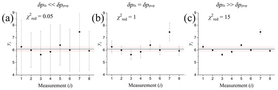
Figure 1. A constant statistical model fits eight data points with different errors: (a) when the errors are too large (overestimation), the reduced chi-square is less than 1, the fitted line that represents the average of data points (black line) does pass through all the data points or their error lines, but the variation in the fitted model (red lines) is small compared to the size of errors, leading to a meaningless rate of good fitting. (c) When the errors are too small (underestimation), the calculated reduced chi-square is more than 1, and the fitted line does not pass through all the data points or their error lines, leading to an obvious bad fitting. (b) In the case where the errors are similar to the deviations of the data points from the model, the reduced chi-square is about 1, and the fitting is characterized as good.

In particular, Figure 1 shows the fitting of eight data values with a constant fitting model (a special case of a linear model is shown in detail in Section 2.1; see: [10,11,12]). This fitting is performed to test the statistical hypothesis that the data values are well represented by a constant. The characterization of the fitting depends on the accompanying observational uncertainties. Too large uncertainties (Figure 1a) lead to small value of the reduced chi-square (${\chi }_{\mathrm{red}}^{\hspace{0.17em}2}<1$); if the fitting model is the right choice, then, this result indicates that there is an error overestimation characterizing the observational data. On the other hand, too small uncertainties (Figure 1c) lead to a large value of the reduced chi-square (${\chi }_{\mathrm{red}}^{\hspace{0.17em}2}>1$); again, if the fitting model is the right choice, then, this outcome indicates that there is an error underestimation of the observational data. The optimal fitting goodness would be for observation uncertainties similar to the data variation (Figure 1b), meaning that the two types of errors are about the same, and the reduced chi-square is about one (${\chi }_{\mathrm{red}}^{\hspace{0.17em}2}~1$).

The statistical behavior of chi-squared values derived from model residuals has been thoroughly understood for over a century, thanks to the foundational work of R.A. Fisher [13,14]. Fisher not only performed the necessary algebraic derivations but also rigorously established the associated probability distributions. Building on this classical framework, the current study introduces a fresh algebraic and intuitive perspective on reduced chi-squared statistics.

The purpose of this paper is to show an alternative perspective to the statistical meaning of the reduced chi-square as a measure of the goodness of fitting methods, and finally, to demonstrate it with several examples and applications. This expression is given by the ratio between the two types of errors, the fitting over the propagation error, which holds for any linearly parameterized fitting. We show this characterization of chi-square, as follows. We first work with the traditional examples of one-parametric fitting of a constant and the bi-parametric fitting of a linear model; then, we provide the proof for the general case of any linearly multi-parameterized model. Nevertheless, we present a counterexample of this characterization of chi-square, showing that it is not generally true for nonlinearly parameterized fitting. Furthermore, we focus on the nature of the two types of errors and show their independent origin. We also examine how the observation uncertainties affect the formulations of the fitting and propagation errors and the reduced chi-square. The developments of this paper in regard to the chi-square formulation and characterization are applied in the case of plasma protons of the heliosheath; we find that the acceptable characterization of the fitting goodness is given by one order of magnitude of the reduced chi-square around its optimal unity value, $0.1<{\chi }_{\mathrm{red}}^{\hspace{0.17em}2}<10$.

The paper is organized as follows: In Section 2, we show both the cases of linearly and nonlinearly parametric fitting models. We start with a linearly mono-parametric model, then work with bi-parametric model, and end up with the general case of a multi-parametric fitting model of an arbitrary number of independent parameters. In the same section, we show that the reduced chi-square cannot be used for nonlinear parametric fitting models. We show this separately for nonlinearly mono-parameterized and multi-parameterized models. In Section 3, we provide an example application from the plasma protons in the heliosphere. Finally, in Section 4, we summarize the conclusions and findings of this paper.

2. Methods

2.1. Linearly Parametrical Fitting

2.1.1. Linearly Mono-Parametric Fitting

The linearly mono-parametric model function can be generally written as

$$f\left(x;p\right)=g_0(x)+p\cdot g_1(x),$$

(11)

where the variable functions g₀(x) and g₁(x) may be linear or nonlinear. Here, we use the simplest case of a constant function, $f\left(x;p\right)=p$. Minimization of the chi-square,

$${\chi }^2\left(p\right)={\displaystyle \sum _{i=1}^N{\left(\frac{y_i-p}{{\sigma }_{yi}}\right)}^{\hspace{0.17em}2}},$$

(12)

involves finding the optimal values of the fitting parameters, $p=p^{*}$, so that

$$p^{*}=\overline{y}={\displaystyle \sum _{i=1}^N\frac{y_i}{{\sigma }_{yi}^{\hspace{0.17em}\hspace{0.17em}\hspace{0.17em}2}}}/{\displaystyle \sum _{i=1}^N\frac{1}{{\sigma }_{yi}^{\hspace{0.17em}\hspace{0.17em}\hspace{0.17em}2}}}.$$

(13)

In order to derive the fitting error, the chi-square is expanded near its minimum,

$${\chi }^2\left(p\right)\cong A_0+A_2\cdot {(p-p^{*})}^{\hspace{0.17em}2}+O{(p-p^{*})}^{\hspace{0.17em}3}.$$

(14)

The square of the fitting error is proportional to the (reduced) chi-square and inversely proportional to the curvature coefficient A₂ [5], i.e.,

$$\delta p_{\hspace{0.17em}\hspace{0.17em}\hspace{0.17em}\hspace{0.17em}\mathrm{fit}}^{*}=\sqrt{\frac{1}{N-1}{A}_0\cdot A_2^{-1}},$$

(15)

where $A_0={\chi }^2(p^{*})$ is the minimum chi-square and $\frac{1}{N-1}{A}_0={\chi }_{\mathrm{red}}^2$ is the reduced chi-square. For more details, see [5]. In our case, the expansion of the chi-square, given by Equation (14), is

$${\chi }^2\left(p\right)={\displaystyle \sum _{i=1}^N{\left[\frac{(y_i-p^{*})-(p-p^{*})}{{\sigma }_{yi}}\right]}^{\hspace{0.17em}2}}={\chi }^2\left(p^{*}\right)+\left({\displaystyle \sum _{i=1}^N\frac{1}{{\sigma }_{yi}^{\hspace{0.17em}\hspace{0.17em}\hspace{0.17em}2}}}\right)\cdot {(p-p^{*})}^{\hspace{0.17em}2}.$$

(16)

Hence, the curvature coefficient equals

$$A_2={\displaystyle \sum _{i=1}^N\frac{1}{{\sigma }_{yi}^{\hspace{0.17em}\hspace{0.17em}\hspace{0.17em}2}}},$$

(17)

thus, the fitting error equals

$$\delta p_{\hspace{0.17em}\hspace{0.17em}\hspace{0.17em}\hspace{0.17em}\mathrm{fit}}^{*}=\sqrt{{\chi }_{\mathrm{red}}^2}/\sqrt{{\displaystyle \sum _{i=1}^N\frac{1}{{\sigma }_{yi}^{\hspace{0.17em}\hspace{0.17em}\hspace{0.17em}2}}}}.$$

(18)

The origin of the fitting error comes from the residuals, i.e., the deviations between the data and model, ${\{\hspace{0.17em}{y}_i-f_i\}}_{i=1}^N$. The role of the observational uncertainties of the data, ${\left\{{\sigma }_{yi}\right\}}_{i=1}^N$, in the formulation of this deviation, is simply to express the statistical weights. They do not contribute to the measures of these deviations. For example, if all the observational uncertainties were equal, either big or small, then, they would have always zero impact on the value of the fitting error. Indeed, if ${\{\hspace{0.17em}{\sigma }_{yi}=\sigma \}}_{i=1}^N$, then,

$$\delta p_{\hspace{0.17em}\hspace{0.17em}\hspace{0.17em}\mathrm{fit}}^{*}=\sqrt{\frac{1}{N(N-1)}\cdot {\displaystyle {\sum }_{i=1}^N{\left(y_i-p^{*}\right)}^2}},$$

(19)

that is, the fitting error becomes independent of the uncertainty σ.

The actual measure of the observational uncertainties comes with the propagation error. This is a type of error different from the fitting error; it generally differs in its nature, origin, and value. The propagation error originates from the function that expresses the optimal value in terms of the observation data, $p^{*}({\left\{y_i\right\}}_{i=1}^N)$. The variation in this function leads to the propagation error,

$$\delta p_{\hspace{0.17em}\hspace{0.17em}\hspace{0.17em}\mathrm{prop}}^{*}=\sqrt{{\displaystyle \sum _{i=1}^N{\left(\frac{\partial p^{*}}{\partial y_i}\right)}^{\hspace{0.17em}2}{\sigma }_{yi}^{\hspace{0.17em}\hspace{0.17em}\hspace{0.17em}2}}}.$$

(20)

In our case, where $p^{*}({\left\{y_i\right\}}_{i=1}^N)=\overline{y}$, the propagation error is specifically equal to

$$\delta p_{\hspace{0.17em}\hspace{0.17em}\hspace{0.17em}\mathrm{prop}}^{*}=1/\sqrt{{\displaystyle \sum _{i=1}^N\frac{1}{{\sigma }_{yi}^{\hspace{0.17em}\hspace{0.17em}\hspace{0.17em}2}}}}.$$

(21)

We note that the square of the propagation error equals the inverse curvature coefficient,

$$\delta p_{\hspace{0.17em}\hspace{0.17em}\hspace{0.17em}\mathrm{fit}}^{*\hspace{0.17em}2}=A_2^{-1},$$

(22)

where we conclude that the chi-square is related to the ratio of the two errors, i.e.,

$$\sqrt{{\chi }_{\mathrm{red}}^2}=\delta p_{\hspace{0.17em}\hspace{0.17em}\hspace{0.17em}\mathrm{fit}}^{*}/\delta p_{\hspace{0.17em}\hspace{0.17em}\hspace{0.17em}\mathrm{prop}}^{*}.$$

(23)

The fitting error is given by the formulation of the standard error, i.e.,

$$\delta {\overline{y}}^{\hspace{0.17em}2}=\frac{1}{N-1}{\displaystyle \sum _{i=1}^N\frac{{(y_i-\overline{y})}^{\hspace{0.17em}2}}{{\sigma }_{yi}^{\hspace{0.17em}\hspace{0.17em}\hspace{0.17em}2}}}/{\displaystyle \sum _{i=1}^N\frac{1}{{\sigma }_{yi}^{\hspace{0.17em}\hspace{0.17em}\hspace{0.17em}2}}}.$$

(24)

Thus, its connection to the reduced chi-square is

$${\chi }_{\mathrm{red}}^2=\frac{1}{N-1}{\displaystyle \sum _{i=1}^N\frac{{(y_i-\overline{y})}^{\hspace{0.17em}2}}{{\sigma }_{yi}^{\hspace{0.17em}\hspace{0.17em}\hspace{0.17em}2}}}=\left({\displaystyle \sum _{i=1}^N\frac{1}{{\sigma }_{yi}^{\hspace{0.17em}\hspace{0.17em}\hspace{0.17em}2}}}\right)\cdot \delta {\overline{y}}^{\hspace{0.17em}2},$$

(25)

or

$$\delta p_{\hspace{0.17em}\hspace{0.17em}\hspace{0.17em}\mathrm{fit}}^{*}=\delta \overline{y}=\sqrt{{\chi }_{\mathrm{red}}^2}/\sqrt{{\displaystyle {\sum }_{i=1}^N{\sigma }_{yi}^{\hspace{0.17em}\hspace{0.17em}\hspace{0.17em}-2}}}, \delta p_{\hspace{0.17em}\hspace{0.17em}\hspace{0.17em}\mathrm{prop}}^{*}=1/\sqrt{{\displaystyle {\sum }_{i=1}^N{\sigma }_{yi}^{\hspace{0.17em}\hspace{0.17em}\hspace{0.17em}-2}}}.$$

(26)

An example of this fitting is shown in Figure 1. Large deviations between propagation and fitting errors lead to a reduced chi-square significantly different than one, corresponding to low fitting goodness.

2.1.2. Linearly Bi-Parametric Fitting

The linearly bi-parametric model function can be written as

$$f\left(x;p_1,p_2\right)=g_0(x)+p_1\cdot g_1(x)+p_2\cdot g_2(x).$$

(27)

As an example, we use the simplest case of a linear function, $f\left(x;p_1,p_2\right)=p_1+p_2\cdot x$, with the fitting parameters of intercept p₁ and slope p₂. Minimization of the chi-square,

$${\chi }^2\left(p_1,p_2\right)={\displaystyle \sum _{i=1}^N{\left(\frac{y_i-p_1-p_2\cdot x_i}{{\sigma }_{yi}}\right)}^{\hspace{0.17em}2}},$$

(28)

leads to the optimal fitting parameters:

$$p_1^{*}=\overline{y}-p_2^{*}\cdot \overline{x}, p_2^{*}={\sigma }_{xy}^2/{\sigma }_{xx}^2.$$

(29)

The minimum value of the chi-square equals

$${\chi }^2\left(p_1^{*},p_2^{*}\right)={\displaystyle \sum _{i=1}^N{\left[\frac{(y_i-\overline{y})-p_2^{*}\cdot (x_i-\overline{x})}{{\sigma }_{yi}}\right]}^{\hspace{0.17em}2}}={\sigma }_{xx}^{-2}\cdot ({\sigma }_{xx}^2{\sigma }_{yy}^2-{\sigma }_{xy}^4)\cdot {\displaystyle \sum _{i=1}^N\frac{1}{{\sigma }_{yi}^{\hspace{0.17em}\hspace{0.17em}\hspace{0.17em}2}}},$$

(30)

where we find

$$\begin{array}{l}{\sigma }_{yy}^2={\displaystyle \sum _{i=1}^N\frac{{(y_i-\overline{y})}^{\hspace{0.17em}2}}{{\sigma }_{yi}^{\hspace{0.17em}\hspace{0.17em}\hspace{0.17em}2}}}/{\displaystyle \sum _{i=1}^N\frac{1}{{\sigma }_{yi}^{\hspace{0.17em}\hspace{0.17em}\hspace{0.17em}2}}}\hspace{0.17em},\\ {\sigma }_{xy}^2={\displaystyle \sum _{i=1}^N\frac{(x_i-\overline{x})(y_i-\overline{y})}{{\sigma }_{yi}^{\hspace{0.17em}\hspace{0.17em}\hspace{0.17em}2}}}/{\displaystyle \sum _{i=1}^N\frac{1}{{\sigma }_{yi}^{\hspace{0.17em}\hspace{0.17em}\hspace{0.17em}2}}}\hspace{0.17em},\\ {\sigma }_{xx}^2={\displaystyle \sum _{i=1}^N\frac{{(x_i-\overline{x})}^{\hspace{0.17em}2}}{{\sigma }_{yi}^{\hspace{0.17em}\hspace{0.17em}\hspace{0.17em}2}}}/{\displaystyle \sum _{i=1}^N\frac{1}{{\sigma }_{yi}^{\hspace{0.17em}\hspace{0.17em}\hspace{0.17em}2}}}\hspace{0.17em},\end{array}$$

(31)

and

$$\overline{x}={\displaystyle \sum _{i=1}^N\frac{x_i}{{\sigma }_{yi}^{\hspace{0.17em}\hspace{0.17em}\hspace{0.17em}2}}}/{\displaystyle \sum _{i=1}^N\frac{1}{{\sigma }_{yi}^{\hspace{0.17em}\hspace{0.17em}\hspace{0.17em}2}}}, \overline{y}={\displaystyle \sum _{i=1}^N\frac{y_i}{{\sigma }_{yi}^{\hspace{0.17em}\hspace{0.17em}\hspace{0.17em}2}}}/{\displaystyle \sum _{i=1}^N\frac{1}{{\sigma }_{yi}^{\hspace{0.17em}\hspace{0.17em}\hspace{0.17em}2}}}.$$

(32)

Next, we calculate the two types of errors. First, we find the propagation error of the optimal slope, which is,

$$\delta p_{2\mathrm{prop}}^{*}=\sqrt{{\displaystyle \sum _{i=1}^N{\left(\frac{\partial p_2^{*}}{\partial y_i}\right)}^{\hspace{0.17em}2}{\sigma }_{yi}^{\hspace{0.17em}\hspace{0.17em}\hspace{0.17em}2}}}={\sigma }_{xx}^{-2}\sqrt{{\displaystyle \sum _{i=1}^N{\left(\frac{\partial {\sigma }_{xy}^2}{\partial y_i}\right)}^{\hspace{0.17em}2}{\sigma }_{yi}^{\hspace{0.17em}\hspace{0.17em}\hspace{0.17em}2}}}.$$

(33)

We have

$${\displaystyle \frac{\partial {\sigma }_{xy}^2}{\partial y_j}}{\sigma }_{yi}={\displaystyle \frac{(x_i-\overline{x})}{{\sigma }_{yi}}}/{\displaystyle \sum _{i=1}^N\frac{1}{{\sigma }_{yi}^{\hspace{0.17em}\hspace{0.17em}\hspace{0.17em}2}}},$$

(34)

or

$${\displaystyle \sum _{j=1}^N{\left(\frac{\partial {\sigma }_{xy}^2}{\partial y_i}\right)}^{\hspace{0.17em}2}{\sigma }_{yi}^{\hspace{0.17em}\hspace{0.17em}\hspace{0.17em}2}}={\displaystyle \sum _{i=1}^N\frac{{(x_i-\overline{x})}^{\hspace{0.17em}2}}{{\sigma }_{yi}^{\hspace{0.17em}\hspace{0.17em}\hspace{0.17em}2}}}/{\left({\displaystyle \sum _{i=1}^N\frac{1}{{\sigma }_{yi}^{\hspace{0.17em}\hspace{0.17em}\hspace{0.17em}2}}}\right)}^{\hspace{0.17em}2}={\sigma }_{xx}^2/\left({\displaystyle \sum _{i=1}^N\frac{1}{{\sigma }_{yi}^{\hspace{0.17em}\hspace{0.17em}\hspace{0.17em}2}}}\right).$$

(35)

Hence, the propagation error of the optimal slope is

$$\delta p_{2\mathrm{prop}}^{*}={\sigma }_{xx}^{-1}\cdot {\left({\displaystyle \sum _{i=1}^N{\sigma }_{yi}^{\hspace{0.17em}\hspace{0.17em}\hspace{0.17em}-2}}\right)}^{-1/2}.$$

(36)

The propagation error of the optimal intercept is

$$\delta p_{1\mathrm{prop}}^{*}=\sqrt{{\displaystyle \sum _{i=1}^N{\left(\frac{\partial p_1^{*}}{\partial y_i}\right)}^{\hspace{0.17em}2}{\sigma }_{yi}^{\hspace{0.17em}\hspace{0.17em}\hspace{0.17em}2}}},$$

(37)

where $p_1^{*}=\overline{y}-p_2^{*}\cdot \overline{x}$; thus, we obtain

$${\displaystyle \frac{\partial p_1^{*}}{\partial y_j}}={\displaystyle \frac{\partial \overline{y}}{\partial y_j}}-{\displaystyle \frac{\partial p_2^{*}}{\partial y_j}}\cdot \overline{x}=\left[1-(x_j-\overline{x})\cdot \overline{x}{\sigma }_{xx}^{-2}\right]{\sigma }_{yj}^{\hspace{0.17em}\hspace{0.17em}\hspace{0.17em}-2}/{\displaystyle \sum _{i=1}^N{\sigma }_{yi}^{\hspace{0.17em}\hspace{0.17em}\hspace{0.17em}-2}},$$

(38)

or

$${\left({\displaystyle \frac{\partial p_1^{*}}{\partial y_j}}\right)}^{\hspace{0.17em}2}{\sigma }_{yj}^{\hspace{0.17em}\hspace{0.17em}\hspace{0.17em}-2}={\left[1-(x_j-\overline{x})\cdot \overline{x}{\sigma }_{xx}^{-2}\right]}^{\hspace{0.17em}2}{\sigma }_{yj}^{\hspace{0.17em}\hspace{0.17em}\hspace{0.17em}-2}/{\left({\displaystyle \sum _{i=1}^N{\sigma }_{yi}^{\hspace{0.17em}\hspace{0.17em}\hspace{0.17em}-2}}\right)}^2,$$

(39)

namely,

$${\displaystyle \sum _{i=1}^N{\left(\frac{\partial p_1^{*}}{\partial y_i}\right)}^{\hspace{0.17em}2}{\sigma }_{yi}^{\hspace{0.17em}\hspace{0.17em}\hspace{0.17em}2}}=(1+{\overline{x}}^{\hspace{0.17em}2}{\sigma }_{xx}^{-2})/{\displaystyle \sum _{i=1}^N{\sigma }_{yi}^{\hspace{0.17em}\hspace{0.17em}\hspace{0.17em}-2}}=\overline{x^{\hspace{0.17em}2}}{\sigma }_{xx}^{-2}/{\displaystyle \sum _{i=1}^N{\sigma }_{yi}^{\hspace{0.17em}\hspace{0.17em}\hspace{0.17em}-2}}.$$

(40)

Hence, we find that the propagation error of the optimal intercept is

$$\delta p_{1\mathrm{prop}}^{*}=\sqrt{\overline{x^{\hspace{0.17em}2}}}\cdot {\sigma }_{xx}^{-1}\cdot {\left({\displaystyle \sum _{i=1}^N{\sigma }_{yi}^{\hspace{0.17em}\hspace{0.17em}\hspace{0.17em}-2}}\right)}^{-1/2}.$$

(41)

Next, we derive the respective fitting errors. For this, we expand the chi-square at its minimum value,

$${\chi }^2\left(p_1,p_2\right)\cong A_0+{\displaystyle \sum _{m=1}^2{\displaystyle \sum _{n=1}^2{(A_2)}_{mn}\cdot (p_m-p_m^{*})(p_n-p_n^{*})}}+O[{(p_m-p_m^{*})}^a{(p_n-p_n^{*})}^b].$$

(42)

ignoring higher terms for $a+b\ge 3$. Then, the chi-square minimum is

$$A_0={\chi }^2\left(p_1^{*},p_2^{*}\right), \frac{1}{N-2}{A}_0={\chi }_{\mathrm{red}}^2,$$

(43)

while the curvature coefficient A₂ is a matrix equal to half the Hessian matrix H [14],

$${(A_2)}_{m\hspace{0.17em}n}=\frac{1}{2}{H}_{mn},$$

(44)

defined by

$$H_{mn}\equiv {\displaystyle \frac{{\partial }^2{\chi }^2\left(p_1^{*},p_2^{*}\right)}{\partial p_m\partial p_n}}.$$

(45)

The curvature coefficient matrix is

$$(A_2)=\left({\displaystyle \sum _{i=1}^N{\sigma }_{yi}^{\hspace{0.17em}\hspace{0.17em}\hspace{0.17em}-2}}\right)\cdot \left(\begin{array}{cc}1& \overline{x}\\ \overline{x}& \overline{x^2}\end{array}\right)\mathrm{or} {(A_2)}^{-1}={\sigma }_{xx}^{\hspace{0.17em}\hspace{0.17em}\hspace{0.17em}-2}{\left({\displaystyle \sum _{i=1}^N{\sigma }_{yi}^{\hspace{0.17em}\hspace{0.17em}\hspace{0.17em}-2}}\right)}^{-1}\cdot \left(\begin{array}{cc}\overline{x^2}& -\overline{x}\\ -\overline{x}& 1\end{array}\right).$$

(46)

Thus,

$${(A_2)}_{11}^{-1}=\overline{x^2}\cdot {\sigma }_{xx}^{\hspace{0.17em}\hspace{0.17em}\hspace{0.17em}-2}\cdot {\left({\displaystyle \sum _{i=1}^N{\sigma }_{yi}^{\hspace{0.17em}\hspace{0.17em}\hspace{0.17em}-2}}\right)}^{-1}\mathrm{and} {(A_2)}_{22}^{-1}={\sigma }_{xx}^{\hspace{0.17em}\hspace{0.17em}\hspace{0.17em}-2}\cdot {\left({\displaystyle \sum _{i=1}^N{\sigma }_{yi}^{\hspace{0.17em}\hspace{0.17em}\hspace{0.17em}-2}}\right)}^{-1}.$$

(47)

Therefore, the fitting errors are given by

$$\delta p_{m\mathrm{fit}}^{*}=\sqrt{\frac{1}{N-2}{A}_0\cdot {(A_2)}_{mm}^{-1}},$$

(48)

or

$$\delta p_{1\mathrm{fit}}^{*}={\sigma }_{xx}^{-2}\cdot \sqrt{\frac{1}{N-2}\overline{x^{\hspace{0.17em}2}}({\sigma }_{xx}^2{\sigma }_{yy}^2-{\sigma }_{xy}^4)}, \delta p_{2\mathrm{fit}}^{*}={\sigma }_{xx}^{-2}\cdot \sqrt{\frac{1}{N-2}({\sigma }_{xx}^2{\sigma }_{yy}^2-{\sigma }_{xy}^4)}.$$

(49)

We observe that the respective propagation errors are

$$\delta p_{1\mathrm{prop}}^{*}=\sqrt{{(A_2)}_{11}^{-1}}\mathrm{and} \delta p_{2\mathrm{prop}}^{*}=\sqrt{{(A_2)}_{22}^{-1}}.$$

(50)

Finally, the ratio of the fitting over the propagation errors, for either the slope or the intercept, provides the chi-square,

$$\delta p_{1\mathrm{prop}}^{*}=\sqrt{{(A_2)}_{11}^{-1}}\mathrm{and} \delta p_{2\mathrm{prop}}^{*}=\sqrt{{(A_2)}_{22}^{-1}}.$$

(51)

which can be given more explicitly through the following formulation:

$${\chi }_{\mathrm{red}}^2=\frac{1}{N-2}\cdot {\sigma }_{xx}^{-2}\cdot ({\sigma }_{xx}^2{\sigma }_{yy}^2-{\sigma }_{xy}^4)\cdot {\displaystyle \sum _{i=1}^N{\sigma }_{yi}^{\hspace{0.17em}\hspace{0.17em}\hspace{0.17em}-2}}.$$

(52)

2.1.3. Linearly Multi-Parametric Fitting

Lastly, in this section, we examine the most general linearly multi-parametric model function, i.e.,

$$f\left(x;{\left\{p_k\right\}}_{k=1}^M\right)={\displaystyle \sum _{k=1}^M{p}_k\cdot g_k(x)}.$$

(53)

that involves the arbitrary nonlinear functions of x, ${\{g_k(x)\}}_{k=1}^M$. (Note that in this compact version of Equation (53), we have included the former function $g_0(x)$ in the sum with p₀ = 1.)

The chi-square is now formulated by

$${\chi }^2\left({\left\{p_k\right\}}_{k=1}^M\right)={\displaystyle \sum _{i=1}^N{\left[\frac{y_i-{\displaystyle \sum _{k=1}^M{p}_k\cdot g_k(x_i)}}{{\sigma }_{yi}}\right]}^{\hspace{0.17em}2}}.$$

(54)

The expansion around its minimum is

$${\chi }^2\left({\left\{p_k\right\}}_{k=1}^M\right)\cong A_0+{\displaystyle \sum _{m=1}^M{\displaystyle \sum _{n=1}^M{(A_2)}_{mn}\cdot (p_m-p_m^{*})(p_n-p_n^{*})}}+O[{(p_m-p_m^{*})}^a{(p_n-p_n^{*})}^b],$$

(55)

where the minimum chi-square value is given by

$$A_0={\chi }^2\left({\left\{p_k^{*}\right\}}_{k=1}^M\right), \frac{1}{N-M}{A}_0={\chi }_{\mathrm{red}}^2,$$

(56)

while the curvature coefficient A₂ is a matrix equal to half the Hessian matrix H,

$${(A_2)}_{mn}=\frac{1}{2}{H}_{mn}, H_{mn}\equiv {\displaystyle \frac{{\partial }^2{\chi }^2\left({\left\{p_k^{*}\right\}}_{k=1}^M\right)}{\partial p_m\partial p_n}}.$$

(57)

The minimization of the chi-square, that is,

$${\displaystyle \frac{\partial {\chi }^2\left({\left\{p_k\right\}}_{k=1}^M\right)}{\partial p_m}}=-2{\displaystyle \sum _{i=1}^N\left[\frac{y_i-{\displaystyle \sum _{k=1}^M{p}_k\cdot g_k(x_i)}}{{\sigma }_{yi}^{\hspace{0.17em}\hspace{0.17em}\hspace{0.17em}2}}\right]\cdot g_m(x_i)}=0,$$

(58)

leads to the optimal values of the parameters, which are implicitly given by

$${\displaystyle \sum _{i=1}^N\frac{y_i\hspace{0.17em}{g}_m(x_i)}{{\sigma }_{yi}^{\hspace{0.17em}\hspace{0.17em}\hspace{0.17em}2}}}={\displaystyle \sum _{k=1}^M{p}_k^{*}\cdot }{\displaystyle \sum _{i=1}^N\frac{g_k(x_i)g_m(x_i)}{{\sigma }_{yi}^{\hspace{0.17em}\hspace{0.17em}\hspace{0.17em}2}}}.$$

(59)

Note that the argument ${\displaystyle {\sum }_{i=1}^N{\sigma }_{yi}^{\hspace{0.17em}\hspace{0.17em}\hspace{0.17em}-2}{g}_a(x_i)g_b(x_i)}$ is a matrix (two free indices, a and b), which is connected with Hessian matrix. Indeed, the Hessian or curvature matrix is derived from differentiating Equation (58) once more, that is,

$${(A_2)}_{mn}=\frac{1}{2}{H}_{mn}=\frac{1}{2}{\displaystyle \frac{{\partial }^2{\chi }^2\left({\left\{p_k\right\}}_{k=1}^M\right)}{\partial p_m\partial p_n}}={\displaystyle \sum _{i=1}^N\frac{g_m(x_i)g_n(x_i)}{{\sigma }_{yi}^{\hspace{0.17em}\hspace{0.17em}\hspace{0.17em}2}}}.$$

(60)

Hence, we observe that Equation (59) can be written in terms of the curvature matrix, i.e.,

$${\displaystyle \sum _{i=1}^N\frac{y_i\hspace{0.17em}{g}_m(x_i)}{{\sigma }_{yi}^{\hspace{0.17em}\hspace{0.17em}\hspace{0.17em}2}}}={\displaystyle \sum _{k=1}^M{p}_k^{*}\cdot {(A_2)}_{km}}.$$

(61)

Some calculations lead to

$${\displaystyle \sum _{i=1}^N\left[\frac{y_i\hspace{0.17em}}{{\sigma }_{yi}^{\hspace{0.17em}\hspace{0.17em}\hspace{0.17em}2}}\hspace{0.17em}{\displaystyle \sum _{m=1}^M{g}_m(x_i){(A_2)}_{m\hspace{0.17em}n}^{-1}}\right]}={\displaystyle \sum _{k=1}^M{p}_k^{*}\cdot {\displaystyle \sum _{m=1}^M{(A_2)}_{km}{(A_2)}_{m\hspace{0.17em}n}^{-1}}}={\displaystyle \sum _{k=1}^M{p}_k^{*}{\delta }_{kn}}=p_n^{*},$$

(62)

and

$$\begin{array}{l}{\left({\displaystyle \frac{\partial p_n^{*}}{\partial y_j}}\right)}^{\hspace{0.17em}2}{\sigma }_{yj}^{\hspace{0.17em}\hspace{0.17em}\hspace{0.17em}2}={\sigma }_{yj}^{\hspace{0.17em}\hspace{0.17em}\hspace{0.17em}2}{\left[{\displaystyle \sum _{m=1}^M{g}_m(x_j){(A_2)}_{m\hspace{0.17em}n}^{-1}}\right]}^{\hspace{0.17em}2}\\ ={\sigma }_{yj}^{\hspace{0.17em}\hspace{0.17em}\hspace{0.17em}2}{\displaystyle \sum _{m=1}^M{\displaystyle \sum _{m^{\prime }=1}^M{g}_m(x_j)g_{m^{\prime }}(x_j){(A_2)}_{m\hspace{0.17em}n}^{-1}{(A_2)}_{m^{\prime }\hspace{0.17em}n}^{-1}}}\hspace{0.17em}\hspace{0.17em},\end{array}$$

(63)

thus,

$$\begin{array}{l}{\displaystyle \sum _{j=1}^N{\left(\frac{\partial p_n^{*}}{\partial y_j}\right)}^{\hspace{0.17em}2}{\sigma }_{yj}^{\hspace{0.17em}\hspace{0.17em}\hspace{0.17em}2}}={\displaystyle \sum _{m=1}^M{\displaystyle \sum _{m^{\prime }=1}^M\left[{\displaystyle \sum _{j=1}^N\frac{g_m(x_j)g_{m^{\prime }}(x_j)}{{\sigma }_{yj}^{\hspace{0.17em}\hspace{0.17em}\hspace{0.17em}2}}}\right]{(A_2)}_{m\hspace{0.17em}n}^{-1}{(A_2)}_{m^{\prime }\hspace{0.17em}n}^{-1}}}\\ ={\displaystyle \sum _{m=1}^M{\displaystyle \sum _{m^{\prime }=1}^M{(A_2)}_{mm\prime }{(A_2)}_{m\hspace{0.17em}n}^{-1}{(A_2)}_{m^{\prime }\hspace{0.17em}n}^{-1}}}={\displaystyle \sum _{m=1}^M{\delta }_{mn}{(A_2)}_{mn\hspace{0.17em}}^{-1}}={(A_2)}_{nn\hspace{0.17em}}^{-1}\hspace{0.17em}\hspace{0.17em},\end{array}$$

(64)

leading to

$$\delta p_{n\mathrm{prop}}^{*}=\sqrt{{(A_2)}_{nn\hspace{0.17em}}^{-1}}.$$

(65)

Given the standard equation of fitting error,

$$\delta p_{n\mathrm{fit}}^{*}=\sqrt{{\chi }_{\mathrm{red}}^2\cdot {(A_2)}_{nn}^{-1}},$$

(66)

with

$${\chi }_{\mathrm{red}}^2=\frac{1}{N-M}{A}_0,$$

(67)

we finally conclude that

$$\delta p_{n\mathrm{fit}}^{*}/\delta p_{n\mathrm{prop}}^{*}=\sqrt{{\chi }_{\mathrm{red}}^2},\hspace{0.17em}\mathrm{for} \mathrm{all} n: 1, \dots , M.$$

(68)

Namely, the ratio of the fitting over the propagation errors is fixed for any of the M fitting parameters and provides (the square root of) the chi-square.

2.2. Nonlinearly Parametric Fitting

2.2.1. Nonlinearly Mono-Parameterized Fitting

We start with the mono-parametric model function $f\left(x;p\right)$, where the chi-square is given by

$${\chi }^2\left(p\right)={\displaystyle \sum _{i=1}^N{\left(\frac{y_i-f\left(x_i;p\right)}{{\sigma }_{yi}}\right)}^{\hspace{0.17em}2}}.$$

(69)

Minimization of the chi-square involves finding the optimal value $p=p^{*}$ that solves the equation

$${\displaystyle \sum _{i=1}^N\frac{y_i-f(x_i;p^{*})}{{\sigma }_{yi}^{\hspace{0.17em}\hspace{0.17em}\hspace{0.17em}2}}\cdot \frac{\partial f(x_i;p^{*})}{\partial p^{*}}}=0.$$

(70)

Applying the partial derivative $\partial /\partial y_j$ to Equation (70), we have

$$\begin{array}{l}{\displaystyle \sum _{i=1}^N\frac{1}{{\sigma }_{yi}^{\hspace{0.17em}\hspace{0.17em}\hspace{0.17em}2}}\cdot \left\{\left[{\delta }_{ij}-\frac{\partial p^{*}}{\partial y_j}\cdot \frac{\partial f(x_i;p^{*})}{\partial p^{*}}\right]\cdot \frac{\partial f(x_i;p^{*})}{\partial p^{*}}+\left[y_i-f(x_i;p^{*})\right]\cdot \frac{\partial p^{*}}{\partial y_j}\cdot \frac{{\partial }^{2}f(x_i;p^{*})}{\partial p^{*2}}\right\}}=0\\ {\displaystyle \frac{1}{{\sigma }_{yj}^{\hspace{0.17em}\hspace{0.17em}\hspace{0.17em}2}}}\cdot {\displaystyle \frac{\partial f(x_j;p^{*})}{\partial p^{*}}}={\displaystyle \frac{\partial p^{*}}{\partial y_j}}\cdot {\displaystyle \sum _{i=1}^N\frac{1}{{\sigma }_{yi}^{\hspace{0.17em}\hspace{0.17em}\hspace{0.17em}2}}\cdot \left\{{\left[\frac{\partial f(x_i;p^{*})}{\partial p^{*}}\right]}^{\hspace{0.17em}2}-\left[y_i-f(x_i;p^{*})\right]\cdot \frac{{\partial }^{2}f(x_i;p^{*})}{\partial p^{*2}}\right\}}\hspace{0.17em}\hspace{0.17em},\end{array}.$$

(71)

Thus, we obtain

$$\delta p_{\hspace{0.17em}\hspace{0.17em}\hspace{0.17em}\mathrm{prop}}^{*}=\sqrt{{\displaystyle \sum _{j=1}^N{\left(\frac{\partial p^{*}}{\partial y_j}\right)}^2{\sigma }_{yj}^{\hspace{0.17em}\hspace{0.17em}\hspace{0.17em}2}}}={\displaystyle \frac{\sqrt{{\displaystyle \sum _{j=1}^N\frac{1}{{\sigma }_{yj}^{\hspace{0.17em}\hspace{0.17em}\hspace{0.17em}2}}\cdot {\left[\frac{\partial f(x_j;p^{*})}{\partial p^{*}}\right]}^{\hspace{0.17em}2}}}}{{\displaystyle \sum _{i=1}^N\frac{1}{{\sigma }_{yi}^{\hspace{0.17em}\hspace{0.17em}\hspace{0.17em}2}}\cdot \left\{{\left[\frac{\partial f(x_i;p^{*})}{\partial p^{*}}\right]}^{\hspace{0.17em}2}-\left[y_i-f(x_i;p^{*})\right]\cdot \frac{{\partial }^{2}f(x_i;p^{*})}{\partial p^{*2}}\right\}}}}.$$

(72)

The respective curvature coefficient is given by

$$A_2=\frac{1}{2}{\displaystyle \frac{{\partial }^2{\chi }^2(p^{*})}{\partial p^{*2}}}={\displaystyle \sum _{i=1}^N\frac{1}{{\sigma }_{yi}^{\hspace{0.17em}\hspace{0.17em}\hspace{0.17em}2}}}\left\{{\left[{\displaystyle \frac{\partial f\left(x_i;p^{*}\right)}{\partial p^{*}}}\right]}^2-\left[y_i-f\left(x_i;p^{*}\right)\right]{\displaystyle \frac{{\partial }^{2}f\left(x_i;p^{*}\right)}{\partial p^{*2}}}\right\},$$

(73)

which can be included in the expression of propagation error, as follows:

$$\delta p_{\hspace{0.17em}\hspace{0.17em}\hspace{0.17em}\mathrm{prop}}^{*}=\sqrt{{(A_2)}^{-1}\cdot \left[1+{(A_2)}^{-1}{\displaystyle \sum _{i=1}^N\frac{y_i-f(x_i;p^{*})}{{\sigma }_{yi}^{\hspace{0.17em}\hspace{0.17em}\hspace{0.17em}2}}\cdot \frac{{\partial }^{2}f(x_i;p^{*})}{\partial p^{*2}}}\right]},$$

(74)

or

$$\delta p_{\hspace{0.17em}\hspace{0.17em}\hspace{0.17em}\mathrm{prop}}^{*}=\sqrt{{(A_2)}^{-1}+{(A_2)}^{-2}{\displaystyle \sum _{i=1}^N\frac{y_i-f(x_i;p^{*})}{{\sigma }_{yi}^{\hspace{0.17em}\hspace{0.17em}\hspace{0.17em}2}}\cdot \frac{{\partial }^{2}f(x_i;p^{*})}{\partial p^{*2}}}}.$$

(75)

Then, we find that the relationship of the two errors, propagation and fitting, involves the reduced chi-square of the nonlinearly parameterized fitting, ${\chi }_{\mathrm{red},\mathrm{NL}}^2$; however, the relationship is not universal:

$$\delta p_{\hspace{0.17em}\hspace{0.17em}\mathrm{prop}}^{*\hspace{0.17em}\hspace{0.17em}2}=\delta p_{\hspace{0.17em}\hspace{0.17em}\mathrm{fit}}^{*\hspace{0.17em}\hspace{0.17em}2}/{\chi }_{\mathrm{red},\mathrm{NL}}^2+{(A_2)}^{-2}{\displaystyle \sum _{i=1}^N\frac{y_i-f(x_i;p^{*})}{{\sigma }_{yi}^{\hspace{0.17em}\hspace{0.17em}\hspace{0.17em}2}}\cdot \frac{{\partial }^{2}f(x_i;p^{*})}{\partial p^{*2}}}\ne \delta p_{\mathrm{fit}}^{*\hspace{0.17em}\hspace{0.17em}2}/{\chi }_{\mathrm{red},\mathrm{NL}}^2.$$

(76)

Therefore, the chi-square cannot be expressed through the ratio of these errors; thus, there is no universal value of the best chi-square.

2.2.2. Nonlinearly Multi-Parameterized Fitting

The counterexample of the mono-parametric case is enough to show that the chi-square is a meaningless tool for characterizing the goodness of a nonlinearly parameterized fit. Nevertheless, we extend this example to the case of a multi-parametric model function $f\left(x;{\left\{p_k\right\}}_{k=1}^M\right)$.

Minimization of the chi-square,

$$\delta p_{\hspace{0.17em}\hspace{0.17em}\hspace{0.17em}\mathrm{prop}}^{*}=\sqrt{{(A_2)}^{-1}+{(A_2)}^{-2}{\displaystyle \sum _{i=1}^N\frac{y_i-f(x_i;p^{*})}{{\sigma }_{yi}^{\hspace{0.17em}\hspace{0.17em}\hspace{0.17em}2}}\cdot \frac{{\partial }^{2}f(x_i;p^{*})}{\partial p^{*2}}}},$$

(77)

involves finding the optimal parameter values, ${\{p_k=p_k^{\hspace{0.17em}\hspace{0.17em}\hspace{0.17em}*}\}}_{k=1}^M$, that solve the m = 1, …, M, canonical equations:

$${\left.{\displaystyle \frac{\partial {\chi }^2\left({\left\{p_k\right\}}_{k=1}^M\right)}{\partial p_m}}\right|}_{{\{p_k=p_k^{\hspace{0.17em}\hspace{0.17em}\hspace{0.17em}*}\}}_{k=1}^M}=-2{\displaystyle \sum _{i=1}^N\frac{y_i-f(x_i;{\left\{p_k^{\hspace{0.17em}\hspace{0.17em}\hspace{0.17em}*}\right\}}_{k=1}^M)}{{\sigma }_{yi}^{\hspace{0.17em}\hspace{0.17em}\hspace{0.17em}2}}\cdot \frac{\partial f(x_i;{\left\{p_k^{\hspace{0.17em}\hspace{0.17em}\hspace{0.17em}*}\right\}}_{k=1}^M)}{\partial p_m^{\hspace{0.17em}\hspace{0.17em}\hspace{0.17em}*}}}=0.$$

(78)

Applying the derivative, $\partial /\partial p_n$, once more on the chi-square gives the curvature matrix

$$\begin{array}{l}{(A_2)}_{mn}={\displaystyle \sum _{i=1}^N\frac{1}{{\sigma }_{yi}^{\hspace{0.17em}\hspace{0.17em}\hspace{0.17em}2}}\cdot \left\{\begin{array}{l}\frac{\partial f(x_i;{\left\{p_k^{\hspace{0.17em}\hspace{0.17em}\hspace{0.17em}*}\right\}}_{k=1}^M)}{\partial p_m^{\hspace{0.17em}\hspace{0.17em}\hspace{0.17em}*}}\cdot \frac{\partial f(x_i;{\left\{p_k^{\hspace{0.17em}\hspace{0.17em}\hspace{0.17em}*}\right\}}_{k=1}^M)}{\partial p_n^{\hspace{0.17em}\hspace{0.17em}\hspace{0.17em}*}}\\ -\left[y_i-f(x_i;{\left\{p_k^{\hspace{0.17em}\hspace{0.17em}\hspace{0.17em}*}\right\}}_{k=1}^M)\right]\cdot \frac{{\partial }^{2}f(x_i;{\left\{p_k^{\hspace{0.17em}\hspace{0.17em}\hspace{0.17em}*}\right\}}_{k=1}^M)}{\partial p_m^{\hspace{0.17em}\hspace{0.17em}\hspace{0.17em}*}\partial p_n^{\hspace{0.17em}\hspace{0.17em}\hspace{0.17em}*}}\end{array}\right\}}\\ \end{array},$$

(79)

while the derivative $\partial /\partial y_j$ on the optimal parameter values, as shown in Equation (78), gives

$${\displaystyle \sum _{i=1}^N\frac{1}{{\sigma }_{yi}^{\hspace{0.17em}\hspace{0.17em}\hspace{0.17em}2}}\cdot \left\{\begin{array}{l}\left[{\delta }_{ij}-{\displaystyle \sum _{k=1}^M\frac{\partial p_k^{\hspace{0.17em}\hspace{0.17em}\hspace{0.17em}*}}{\partial y_j}\frac{\partial f(x_i;{\left\{p_k^{\hspace{0.17em}\hspace{0.17em}\hspace{0.17em}*}\right\}}_{k=1}^M)}{\partial p_k^{\hspace{0.17em}\hspace{0.17em}\hspace{0.17em}*}}}\right]\cdot \frac{\partial f(x_i;{\left\{p_k^{\hspace{0.17em}\hspace{0.17em}\hspace{0.17em}*}\right\}}_{k=1}^M)}{\partial p_m^{\hspace{0.17em}\hspace{0.17em}\hspace{0.17em}*}}\\ +\left[y_i-f(x_i;{\left\{p_k^{\hspace{0.17em}\hspace{0.17em}\hspace{0.17em}*}\right\}}_{k=1}^M)\right]\cdot {\displaystyle \sum _{k=1}^M\frac{\partial p_k^{\hspace{0.17em}\hspace{0.17em}\hspace{0.17em}*}}{\partial y_j}\frac{{\partial }^{2}f(x_i;{\left\{p_k^{\hspace{0.17em}\hspace{0.17em}\hspace{0.17em}*}\right\}}_{k=1}^M)}{\partial p_k^{\hspace{0.17em}\hspace{0.17em}\hspace{0.17em}*}\partial p_m^{\hspace{0.17em}\hspace{0.17em}\hspace{0.17em}*}}}\end{array}\right\}}=0,$$

(80)

or

$$\begin{array}{l}{\displaystyle \frac{1}{{\sigma }_{yj}^{\hspace{0.17em}\hspace{0.17em}\hspace{0.17em}2}}}\cdot {\displaystyle \frac{\partial f(x_j;{\left\{p_k^{\hspace{0.17em}\hspace{0.17em}\hspace{0.17em}*}\right\}}_{k=1}^M)}{\partial p_m^{\hspace{0.17em}\hspace{0.17em}\hspace{0.17em}*}}}={\displaystyle \sum _{i=1}^N\frac{1}{{\sigma }_{yi}^{\hspace{0.17em}\hspace{0.17em}\hspace{0.17em}2}}\cdot \left\{\begin{array}{l}\left[{\displaystyle \sum _{l=1}^M\frac{\partial p_l^{\hspace{0.17em}\hspace{0.17em}\hspace{0.17em}*}}{\partial y_j}\frac{\partial f(x_i;{\left\{p_k^{\hspace{0.17em}\hspace{0.17em}\hspace{0.17em}*}\right\}}_{k=1}^M)}{\partial p_l^{\hspace{0.17em}\hspace{0.17em}\hspace{0.17em}*}}}\right]\cdot \frac{\partial f(x_i;{\left\{p_k^{\hspace{0.17em}\hspace{0.17em}\hspace{0.17em}*}\right\}}_{k=1}^M)}{\partial p_m^{\hspace{0.17em}\hspace{0.17em}\hspace{0.17em}*}}\\ -\left[y_i-f(x_i;{\left\{p_k^{\hspace{0.17em}\hspace{0.17em}\hspace{0.17em}*}\right\}}_{k=1}^M)\right]\cdot {\displaystyle \sum _{l=1}^M\frac{\partial p_l^{\hspace{0.17em}\hspace{0.17em}\hspace{0.17em}*}}{\partial y_j}\frac{{\partial }^{2}f(x_i;{\left\{p_k^{\hspace{0.17em}\hspace{0.17em}\hspace{0.17em}*}\right\}}_{k=1}^M)}{\partial p_l^{\hspace{0.17em}\hspace{0.17em}\hspace{0.17em}*}\partial p_m^{\hspace{0.17em}\hspace{0.17em}\hspace{0.17em}*}}}\end{array}\right\}}\\ ={\displaystyle \sum _{l=1}^M\frac{\partial p_l^{\hspace{0.17em}\hspace{0.17em}\hspace{0.17em}*}}{\partial y_j}}\cdot {\displaystyle \sum _{i=1}^N\frac{1}{{\sigma }_{yi}^{\hspace{0.17em}\hspace{0.17em}\hspace{0.17em}2}}\cdot \left\{\begin{array}{l}\frac{\partial f(x_i;{\left\{p_k^{\hspace{0.17em}\hspace{0.17em}\hspace{0.17em}*}\right\}}_{k=1}^M)}{\partial p_l^{\hspace{0.17em}\hspace{0.17em}\hspace{0.17em}*}}\cdot \frac{\partial f(x_i;{\left\{p_k^{\hspace{0.17em}\hspace{0.17em}\hspace{0.17em}*}\right\}}_{k=1}^M)}{\partial p_m^{\hspace{0.17em}\hspace{0.17em}\hspace{0.17em}*}}\\ -\left[y_i-f(x_i;{\left\{p_k^{\hspace{0.17em}\hspace{0.17em}\hspace{0.17em}*}\right\}}_{k=1}^M)\right]\cdot \frac{{\partial }^{2}f(x_i;{\left\{p_k^{\hspace{0.17em}\hspace{0.17em}\hspace{0.17em}*}\right\}}_{k=1}^M)}{\partial p_l^{\hspace{0.17em}\hspace{0.17em}\hspace{0.17em}*}\partial p_m^{\hspace{0.17em}\hspace{0.17em}\hspace{0.17em}*}}\end{array}\right\}={\displaystyle \sum _{l=1}^M\frac{\partial p_l^{\hspace{0.17em}\hspace{0.17em}\hspace{0.17em}*}}{\partial y_j}}\cdot {(A_2)}_{lm}}\hspace{0.17em}\hspace{0.17em},\end{array}$$

(81)

where the curvature matrix is given by Equation (79). Then, inversing Equation (81), we obtain

$${\displaystyle \frac{\partial p_n^{\hspace{0.17em}\hspace{0.17em}\hspace{0.17em}*}}{\partial y_j}}={\displaystyle \frac{1}{{\sigma }_{yj}^{\hspace{0.17em}\hspace{0.17em}\hspace{0.17em}2}}}\cdot {\displaystyle \sum _{m=1}^M\left[\frac{\partial f(x_j;{\left\{p_k^{\hspace{0.17em}\hspace{0.17em}\hspace{0.17em}*}\right\}}_{k=1}^M)}{\partial p_m^{\hspace{0.17em}\hspace{0.17em}\hspace{0.17em}*}}\right]\cdot {(A_2)}_{mn}^{-1}}.$$

(82)

Then, we derive the propagation error, as follows:

$$\delta p_{n\mathrm{prop}}^{*\hspace{0.17em}\hspace{0.17em}2}={\displaystyle \sum _{i=1}^N{\left(\frac{\partial p_n^{\hspace{0.17em}\hspace{0.17em}\hspace{0.17em}*}}{\partial y_i}\right)}^{\hspace{0.17em}2}{\sigma }_{yi}^{\hspace{0.17em}\hspace{0.17em}\hspace{0.17em}2}}={\displaystyle \sum _{i=1}^N\left\{\frac{1}{{\sigma }_{yi}^{\hspace{0.17em}\hspace{0.17em}\hspace{0.17em}2}}\cdot {\left\{{\displaystyle \sum _{m=1}^M\left[\frac{\partial f(x_i;{\left\{p_k^{\hspace{0.17em}\hspace{0.17em}\hspace{0.17em}*}\right\}}_{k=1}^M)}{\partial p_m^{\hspace{0.17em}\hspace{0.17em}\hspace{0.17em}*}}\right]\cdot {(A_2)}_{mn}^{-1}}\right\}}^{\hspace{0.17em}2}\right\}}.$$

(83)

After some calculations, we have

$$\begin{array}{l}{\left\{{\displaystyle \sum _{m=1}^M\left[\frac{\partial f(x_i;{\left\{p_k^{\hspace{0.17em}\hspace{0.17em}\hspace{0.17em}*}\right\}}_{k=1}^M)}{\partial p_m^{\hspace{0.17em}\hspace{0.17em}\hspace{0.17em}*}}\right]\cdot {(A_2)}_{mn}^{-1}}\right\}}^{\hspace{0.17em}2}=\\ {\displaystyle \sum _{m=1}^M{\displaystyle \sum _{m^{\prime }=1}^M\frac{\partial f(x_i;{\left\{p_k^{\hspace{0.17em}\hspace{0.17em}\hspace{0.17em}*}\right\}}_{k=1}^M)}{\partial p_m^{\hspace{0.17em}\hspace{0.17em}\hspace{0.17em}*}}\frac{\partial f(x_i;{\left\{p_k^{\hspace{0.17em}\hspace{0.17em}\hspace{0.17em}*}\right\}}_{k=1}^M)}{\partial p_{m^{\prime }}^{\hspace{0.17em}\hspace{0.17em}\hspace{0.17em}*}}\cdot {(A_2)}_{mn}^{-1}{(A_2)}_{m^{\prime }n}^{-1}}}\hspace{0.17em},\end{array}$$

(84)

and

$$\begin{array}{l}{\displaystyle \sum _{i=1}^N\left\{\frac{1}{{\sigma }_{yi}^{\hspace{0.17em}\hspace{0.17em}\hspace{0.17em}2}}\cdot {\left\{{\displaystyle \sum _{m=1}^M\left[\frac{\partial f(x_i;{\left\{p_k^{\hspace{0.17em}\hspace{0.17em}\hspace{0.17em}*}\right\}}_{k=1}^M)}{\partial p_m^{\hspace{0.17em}\hspace{0.17em}\hspace{0.17em}*}}\right]\cdot [{(A_2)}_{mn}^{-1}]}\right\}}^{\hspace{0.17em}2}\right\}}=\\ {\displaystyle \sum _{m=1}^M{\displaystyle \sum _{m^{\prime }=1}^M\left[{\displaystyle \sum _{i=1}^N\frac{1}{{\sigma }_{yi}^{\hspace{0.17em}\hspace{0.17em}\hspace{0.17em}2}}\cdot \frac{\partial f(x_i;{\left\{p_k^{\hspace{0.17em}\hspace{0.17em}\hspace{0.17em}*}\right\}}_{k=1}^M)}{\partial p_m^{\hspace{0.17em}\hspace{0.17em}\hspace{0.17em}*}}\frac{\partial f(x_i;{\left\{p_k^{\hspace{0.17em}\hspace{0.17em}\hspace{0.17em}*}\right\}}_{k=1}^M)}{\partial p_{m^{\prime }}^{\hspace{0.17em}\hspace{0.17em}\hspace{0.17em}*}}}\right]\cdot {(A_2)}_{mn}^{-1}{(A_2)}_{m^{\prime }n}^{-1}}}\hspace{0.17em}.\end{array}$$

(85)

Hence,

$$\begin{array}{l}\delta p_{n\mathrm{prop}}^{*\hspace{0.17em}\hspace{0.17em}2}={\displaystyle \sum _{i=1}^N{\left(\frac{\partial p_n^{\hspace{0.17em}\hspace{0.17em}\hspace{0.17em}*}}{\partial y_i}\right)}^{\hspace{0.17em}2}{\sigma }_{yi}^{\hspace{0.17em}\hspace{0.17em}\hspace{0.17em}2}}=\\ {\displaystyle \sum _{m=1}^M{\displaystyle \sum _{m^{\prime }=1}^M\left[{\displaystyle \sum _{i=1}^N\frac{1}{{\sigma }_{yi}^{\hspace{0.17em}\hspace{0.17em}\hspace{0.17em}2}}\cdot \frac{\partial f(x_i;{\left\{p_k^{\hspace{0.17em}\hspace{0.17em}\hspace{0.17em}*}\right\}}_{k=1}^M)}{\partial p_m^{\hspace{0.17em}\hspace{0.17em}\hspace{0.17em}*}}\frac{\partial f(x_i;{\left\{p_k^{\hspace{0.17em}\hspace{0.17em}\hspace{0.17em}*}\right\}}_{k=1}^M)}{\partial p_{m^{\prime }}^{\hspace{0.17em}\hspace{0.17em}\hspace{0.17em}*}}}\right]\cdot {(A_2)}_{mn}^{-1}{(A_2)}_{m^{\prime }n}^{-1}}}\hspace{0.17em},\end{array}$$

(86)

or

$$\begin{array}{l}\delta p_{n\mathrm{prop}}^{*\hspace{0.17em}\hspace{0.17em}2}={\displaystyle \sum _{m=1}^M{\displaystyle \sum _{m^{\prime }=1}^M\left\{\begin{array}{l}{(A_2)}_{mm\prime }+\\ {\displaystyle \sum _{i=1}^N\frac{1}{{\sigma }_{yi}^{\hspace{0.17em}\hspace{0.17em}\hspace{0.17em}2}}\cdot [y_i-f(x_i;{\left\{p_k^{\hspace{0.17em}\hspace{0.17em}\hspace{0.17em}*}\right\}}_{k=1}^M)]\cdot \frac{{\partial }^{2}f(x_i;{\left\{p_k^{\hspace{0.17em}\hspace{0.17em}\hspace{0.17em}*}\right\}}_{k=1}^M)}{\partial p_m^{\hspace{0.17em}\hspace{0.17em}\hspace{0.17em}*}\partial p_{m^{\prime }}^{\hspace{0.17em}\hspace{0.17em}\hspace{0.17em}*}}}\end{array}\right\}\cdot {(A_2)}_{mn}^{-1}{(A_2)}_{m^{\prime }n}^{-1}}}\\ ={(A_2)}_{nn}^{-1}+{\displaystyle \sum _{m=1}^M{\displaystyle \sum _{m^{\prime }=1}^M\left\{{\displaystyle \sum _{i=1}^N\frac{1}{{\sigma }_{yi}^{\hspace{0.17em}\hspace{0.17em}\hspace{0.17em}2}}\cdot [y_i-f(x_i;{\left\{p_k^{\hspace{0.17em}\hspace{0.17em}\hspace{0.17em}*}\right\}}_{k=1}^M)]\cdot \frac{{\partial }^{2}f(x_i;{\left\{p_k^{\hspace{0.17em}\hspace{0.17em}\hspace{0.17em}*}\right\}}_{k=1}^M)}{\partial p_m^{\hspace{0.17em}\hspace{0.17em}\hspace{0.17em}*}\partial p_{m^{\prime }}^{\hspace{0.17em}\hspace{0.17em}\hspace{0.17em}*}}}\right\}{(A_2)}_{mn}^{-1}{(A_2)}_{m^{\prime }n}^{-1}}}\hspace{0.17em}\hspace{0.17em}.\end{array}$$

(87)

Therefore,

$$\begin{array}{l}\delta p_{n\mathrm{prop}}^{*\hspace{0.17em}\hspace{0.17em}2}=\delta p_{n\mathrm{fit}}^{*\hspace{0.17em}\hspace{0.17em}2}/{\chi }_{\mathrm{red},\mathrm{NL}}^2+\\ {\displaystyle \sum _{m=1}^M{\displaystyle \sum _{m^{\prime }=1}^M{(A_2)}_{mn}^{-1}{(A_2)}_{m^{\prime }n}^{-1}{\displaystyle \sum _{i=1}^N\frac{y_i-f(x_i;{\left\{p_k^{\hspace{0.17em}\hspace{0.17em}\hspace{0.17em}*}\right\}}_{k=1}^M)}{{\sigma }_{yi}^{\hspace{0.17em}\hspace{0.17em}\hspace{0.17em}2}}\cdot \frac{{\partial }^{2}f(x_i;{\left\{p_k^{\hspace{0.17em}\hspace{0.17em}\hspace{0.17em}*}\right\}}_{k=1}^M)}{\partial p_m^{\hspace{0.17em}\hspace{0.17em}\hspace{0.17em}*}\partial p_{m^{\prime }}^{\hspace{0.17em}\hspace{0.17em}\hspace{0.17em}*}}}}}\hspace{0.17em},\end{array}$$

(88)

or

$$\delta p_{n\mathrm{prop}}^{*\hspace{0.17em}\hspace{0.17em}2}\ne \delta p_{n\mathrm{fit}}^{*\hspace{0.17em}\hspace{0.17em}2}/{\chi }_{\mathrm{red},\mathrm{NL}}^2.$$

(89)

Namely, in any of the general cases of a fitting with multi-parametric model, the chi-square is not given by the ratio of the respective errors (squares); neither has a universal value, because the difference $\delta p_{n\mathrm{prop}}^{*\hspace{0.17em}\hspace{0.17em}2}-\delta p_{n\mathrm{fit}}^{*\hspace{0.17em}\hspace{0.17em}2}/{\chi }_{\mathrm{red},\mathrm{NL}}^2$ differs from case to case depending on the particular fitting model.

3. Discussion: Application in the Outer Heliosphere

We use the reduced chi-square to characterize the goodness of the fitting involved in the method that determines the thermodynamic parameters of the inner heliosheath, that is, the distant outer shelf of our heliosphere. In addition, we use these datasets to compare the two measures related to the estimated chi-square, the reduced chi-square, and the respective p-value.

The Interstellar Boundary Explorer (IBEX) mission observes energetic neutral atom (ENA) emissions, constructing images of the whole sky every six months [15]. The persistence of these maps and its origins has been studied in detail [16,17]. Using these datasets, Livadiotis et al. [10] derived the sky maps of the temperature T, density n, and other thermodynamic quantities that characterize the plasma protons in the inner heliosheath (see also: [18,19,20]). These authors also showed the negative correlation between the values of temperature and density, which originates from the thermodynamic processes of the plasma.

The sky maps of temperature and density constitute 1800 pixels, each with angular dimensions of 6⁰ × 6⁰, while each map’s grid in longitude and latitude is separated in 60 × 30 pixels. The method used by [11] derives eight (statistically independent) measurements of the logarithms of the temperature and density of each pixel. This is based on fitting kappa distributions on the plasma protons, that is, the distribution function of particle velocities linked to the thermodynamics of space plasma particle populations [21,22,23,24,25,26,27,28,29,30]. Once these eight values (temperature and density) are well-fitted by a constant, then, the respective pixel is assigned by this thermodynamic parameter. Figure 2 shows two examples of these eight measurements of temperature and density values. As is shown in Section 2, the fitting parameter is a constant whose constant is the weighted mean. Both types of errors are plotted together with their weighted mean.

Figure 2. Two pixels’ examples of eight measurements of temperature and density values that characterize the sky map of the plasma protons in the inner heliosheath. The weighted average (black) is plotted together with the ± deviation caused by fitting errors (blue) and propagation errors (red). (Tables show statistical details for each fit.).

The two errors were calculated as follows:

$$\delta p_{\hspace{0.17em}\mathrm{prop}}^{*}\cong {\displaystyle \sum _{i=1}^N{[p^{*}(y_i+{\sigma }_{yi})-p^{*}(y_i)]}^{\hspace{0.17em}2}},$$

(90)

and

$$\delta p_{\hspace{0.17em}\hspace{0.17em}\mathrm{prop}}^{*}\cong {\epsilon }^{-1}\cdot \sqrt{{\displaystyle \sum _{i=1}^N{[p^{*}(y_i+\epsilon \cdot {\sigma }_{yi})-p^{*}(y_i)]}^{\hspace{0.17em}2}}}$$

(91)

for some small value of ε (as this tends to zero, the value of the resultant errors becomes independent of ε).

We repeat the above fitting procedure for eight neighboring pixels in the sky (taken from the annual maps of year 2010; see details in [10]). Figure 3a shows these neighboring pixels in the sky maps of temperature and density. Then, in Figure 3b we plot the derived temperature, density, and respective uncertainties (corresponding to the larger among the two error types). Finally, in Figure 3c we show their mutual relationship, by plotting the density against the temperature (logarithmic values). This is described by a negative correlation relationship, originated by a polytropic process with sub-isothermal polytropic index γ. A polytropic process is described by a power-law relation between temperature and density (i.e., $T\propto n^{\gamma -1}$), or between thermal pressure and density (i.e., $p\propto n^{\gamma }$), along a streamline of the flow. In particular, we find a slope $\nu =1/(\gamma -1)$ (that is, the exponent in $n\propto T^{\hspace{0.17em}\nu }$) around ν ~ −2, but it is characterized with better statistics when outlining the last point, leading to ν ~ −1 (also, see: [10,30]).

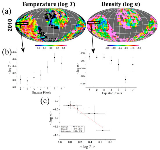
Figure 3. (a) The eight examined neighboring pixels in the sky maps of temperature and density. (b) The results of weighted mean and the uncertainty (largest between fitting and propagation errors). (c) Co-plot of density vs. temperature shows its negative correlation. (Temperature and density are represented with logarithms).

Using the p-value method for evaluating the goodness of fitting [13], we compare the estimated chi-square value, ${\chi }_{\mathrm{est}}^2$, with any possible chi-square value larger than the estimated one, ${\chi }_{\mathrm{est}}^2\le {\chi }^2<\infty$, by deriving this exact probability, $P({\chi }_{\mathrm{est}}^2\le {\chi }^2<\infty )$; this determined the p-value. This is determined by integrating the chi-square distribution, $P({\chi }^2;D)=\frac{2^{-\hspace{0.17em}\frac{D}{2}}}{\Gamma (\frac{D}{2})}\hspace{0.17em}{e}^{-\frac{1}{2}{\chi }^2}{({\chi }^2)}^{\frac{D}{2}-1}$, that is the distribution of all the possible ${\chi }^2$ values (parameterized by the degrees of freedom D). Therefore, the likelihood of having a chi-square value, ${\chi }^2$, larger than the estimated one, ${\chi }_{\mathrm{est}}^2$, is given in terms of the complementary cumulative chi-square distribution. The respective probability, the p-value, equals $P({\chi }_{\mathrm{est}}^2\le {\chi }^2<\infty )={\displaystyle {\int }_{\hspace{0.17em}{\chi }_{\mathrm{est}}^2}^{\hspace{0.17em}\infty }P({\chi }^2;D)\hspace{0.17em}d{\chi }^2}$.

The larger the p-value, the better the goodness of the fitting. A p-value larger than 0.5 corresponds to ${\chi }_{\mathrm{est}}^2$ < D or ${\chi }_{\mathrm{red}}^2$ < 1. Larger p-values, up to p = 1, correspond to smaller chi-squares, down to ${\chi }_{\mathrm{red}}^2$ ~ 0. Thus, an increasing p-value above the threshold of 0.5 cannot lead to a better fitting. Rather, it leads to a worse fit, similar to a decreasing ${\chi }_{\mathrm{red}}^2$ < 1. On the other hand, a p-value smaller than the significance level of ~0.05 is typically rejected. Using these limits of the p-value, we find the respective limits of the reduced chi-square.

In Figure 4, we demonstrate the relationship between the reduced chi-square ${\chi }_{\mathrm{red}}^2$ and the respective p-value P_v. We plot 16 pair values of (${\chi }_{\mathrm{red}}^2$ and P_v), one pair for each of the 16 fitting measures performed (temperature and density fits, both for eight pixels). The deduced relationship between the two measures can be used to deduct the extreme acceptable values of the reduced chi-square; indeed, the best reduced chi-square value that characterizes the goodness of a fitting is one, but at what extreme should a lower goodness be accepted? The correspondence with the acceptable value of 0.05 of the p-value will provide an answer to this issue.

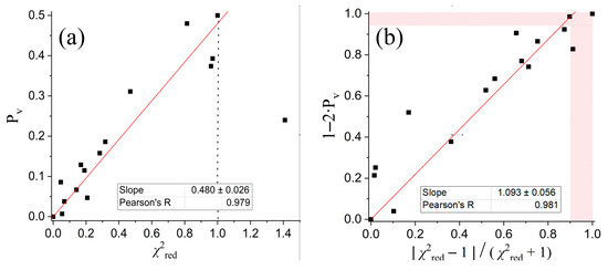
Figure 4. (a) Co-plots of the p-values and the respective reduced chi-square values, showing their relationship. (b) Similar to (a) but with modified functions ranging in [0, 1]; (shaded area corresponds to rejected fits because of low goodness).

In Figure 4a we plot all (${\chi }_{\mathrm{red}}^2$ and P_v) pair values and observe the linear behavior between the two measures. The plot shows the well-described linearity between the low chi-square values ${\chi }_{\mathrm{red}}^2\le 1$ and the corresponding p-values. Nevertheless, in order to also catch the relationship for all the points, including those with ${\chi }_{\mathrm{red}}^2>1$, in Figure 4b we plot the values of 1–2∙P_v as a function of the modified chi-square values, that is, $\left|{\chi }_{\mathrm{red}}^2-1\right|/({\chi }_{\mathrm{red}}^2+1)$, which surely ranges in the interval [0, 1] (similarly for both axes). We find that the excluded p-values (P_v < 0.05) correspond to the reduced chi-square values ${\chi }_{\mathrm{red}}^2<0.1$ and ${\chi }_{\mathrm{red}}^2>10$; (of course, this is not a universal value, but corresponds to the examined datasets).

4. Conclusions

The paper showed the relationship between the two types of errors that characterize the optimal fitting parameters, the fitting and propagation errors. While the fitting error estimates the uncertainty originated from the variation in the observational data around the model, the propagation error comes from the raw uncertainties of the observational data. The (square) ratio of the two errors determines the value of the reduced chi-square.

Large deviations between propagation and fitting errors lead to a reduced chi-square significantly different than one, corresponding to low fitting goodness. In fact, large uncertainties lead to small values of the reduced chi-square (${\chi }_{\mathrm{red}}^{\hspace{0.17em}2}<1$), indicating a possible error overestimation; small uncertainties lead to a large value of the reduced chi-square (${\chi }_{\mathrm{red}}^{\hspace{0.17em}2}>1$), indicating that there is an error underestimation of the observation data. The optimal fitting goodness would be for observation uncertainties similar to the data variation, namely, the two types of errors are about the same, and the reduced chi-square is about one (${\chi }_{\mathrm{red}}^{\hspace{0.17em}2}~1$).

The relationship between the two types of errors and the chi-square was shown for mono-parametric, bi-parametric, and in general, multi-parametric statistical models. In the multi-parametric case, it is interesting that the ratio is universal, namely, independent of the respective parameter; namely, $\delta p_{n\mathrm{fit}}^{*}/\delta p_{n\mathrm{prop}}^{*}=\sqrt{{\chi }_{\mathrm{red}}^2}$, for any n: 1, …, M, as shown in Equation (68).

In addition to this theoretical development, we presented a counterexample of this characterization of chi-square, showing that it is not generally true for a nonlinearly parameterized fitting. Some alternative approaches for assessing nonlinear fits involve the bootstrap inference [31], the Bayesian frameworks [32,33], and the technique of averaging the parameter’s optimal values derived from solving by pairs [11].

Finally, the method of chi-square characterization as a measure of the fitting goodness is applied on the datasets of temperature and density of the plasma protons in the inner heliosheath, the outer shelf of our heliosphere. A previously applied method derived eight measurements of the logarithms of temperature and density for each pixel of the sky map [10]. Once these eight values (temperature and density) are well-fitted by a constant, then, the respective pixel is assigned by this thermodynamic parameter. We have determined the two types of errors of this analysis; the respective reduced chi-square values were compared with the respective p-values for completeness.

References

- Cochran, W.G. The Chi-square Test of Goodness of Fit. Ann. Math. Stat. 1952, 23, 315–345. [Google Scholar] [CrossRef]
- McCullagh, P. What is statistical model? Ann. Stat. 2002, 30, 1225–1310. [Google Scholar] [CrossRef]
- Adèr, H.J. Modelling. In Advising on Research Methods: A Consultant’s Companion; Johannes van Kessel Publishing: Huizen, The Netherlands, 2008; Chapter 12; pp. 271–304. [Google Scholar]
- Burden, R.L.; Faires, J.D. Numerical Analysis; PWS Publishing Company: Boston, MA, USA, 1993; pp. 437–438. [Google Scholar]
- Livadiotis, G. Approach to general fitting methods and their sensitivity. Physica A 2007, 375, 518. [Google Scholar] [CrossRef]
- Livadiotis, G. Chi-p distribution: Characterization of the goodness of the fitting using L p norms. Physica A 2007, 1, 4. [Google Scholar] [CrossRef]
- Frisch, P.C.; Bzowski, M.; Livadiotis, G.; McComas, D.J.; Moebius, E.; Mueller, H.-R.; Pryor, W.R.; Schwadron, N.A.; Sokół, J.M.; Vallerga, J.V.; et al. Decades-long changes of the interstellar wind through our solar system. Science 2013, 341, 1080. [Google Scholar] [CrossRef] [PubMed]
- Shih, J.H.; Fay, M.P. Pearson’s Chi-square Test and Rank Correlation Inferences for Clustered Data. Biometrics 2017, 73, 822–834. [Google Scholar] [CrossRef] [PubMed]
- Bevington, P.R. Data Reduction and Error Analysis for the Physical Sciences; McGraw-Hill: New York, NY, USA, 1969; p. 336. [Google Scholar]
- Livadiotis, G.; McComas, D.J.; Funsten, H.O.; Schwadron, N.A.; Szalay, J.R.; Zirnstein, E. Thermodynamics of the Inner Heliosheath. Astrophys. J. Suppl. Ser. 2022, 262, 53. [Google Scholar] [CrossRef]
- Livadiotis, G.; Cummings, A.T.; Cuesta, M.E.; Bandyopadhyay, R.; Farooki, H.A.; Khoo, L.Y.; McComas, D.J.; Rankin, J.S.; Sharma, T.; Shen, M.M.; et al. Kappa-tail Technique: Modeling and Application to Solar Energetic Particles Observed by Parker Solar Probe. Astrophys. J. Suppl. Ser. 2024, 973, 6. [Google Scholar] [CrossRef]
- Cuesta, M.E.; Cummings, A.T.; Livadiotis, G.; McComas, D.J.; Cohen, C.M.S.; Khoo, L.Y.; Sharma, T.; Shen, M.M.; Bandyopadhyay, R.; Rankin, J.S.; et al. Observations of Kappa Distributions in Solar Energetic Protons and Derived Thermodynamic Properties. Astrophys. J. Suppl. Ser. 2024, 973, 76. [Google Scholar] [CrossRef]
- Fisher, R.A. On the Interpretation of χ2 from Contingency Tables and the Calculation of p. J. R. Stat. Soc. 1922, 85, 87–94. [Google Scholar] [CrossRef]
- Melissinos, A.C. Experiments in Modern Physics; Academic: London, UK, 1966; p. 438. [Google Scholar]
- McComas, D.J.; Allegrini, F.; Bochsler, P.; Bzowski, M.; Christian, E.R.; Crew, G.B.; DeMajistre, R.; Fahr, H.; Fichtner, H.; Frisch, P.C.; et al. Global Observations of the Interstellar Interaction from the Interstellar Boundary Explorer (IBEX). Science 2009, 326, 959. [Google Scholar] [CrossRef]
- Sarlis, N.V.; Livadiotis, G.; McComas, D.J.; Alimaganbetov, M.; Schwadron, N.A.; Fairchild, K. Persistent Behavior in Energetic Neutral Atom Time Series from IBEX. Astrophys. J. Suppl. Ser. 2024, 976, 45. [Google Scholar] [CrossRef]
- Sarlis, N.V.; Livadiotis, G.; McComas, D.J.; Alimaganbetov, M.; Schwadron, N.A. Origins of Persistence in Energetic Neutral Atom Time Series from IBEX. Astrophys. J. Suppl. Ser. 2025, 986, 131. [Google Scholar] [CrossRef]
- Livadiotis, G.; McComas, D.J.; Dayeh, M.A.; Funsten, H.O.; Schwadron, N.A. First Sky Map of the Inner Heliosheath Temperature Using IBEX Spectra. Astrophys. J. Suppl. Ser. 2011, 734, 1. [Google Scholar] [CrossRef]
- Livadiotis, G.; McComas, D.J.; Randol, B.M.; Funsten, H.O.; Möbius, E.S.; Schwadron, N.A.; Dayeh, M.A.; Zank, G.P.; Frisch, P.C. Pick-up Ion Distributions and Their Influence on Energetic Neutral Atom Spectral Curvature. Astrophys. J. Suppl. Ser. 2012, 751, 64. [Google Scholar] [CrossRef]
- Livadiotis, G.; McComas, D.J.; Schwadron, N.A.; Funsten, H.O.; Fuselier, S.A. Pressure of the Proton Plasma in the Inner Heliosheath. Astrophys. J. Suppl. Ser. 2013, 762, 134. [Google Scholar] [CrossRef]
- Livadiotis, G.; McComas, D.J. Beyond kappa distributions: Exploiting Tsallis statistical mechanics in space plasmas. J. Geophys. Res. 2009, 114, A11105. [Google Scholar] [CrossRef]
- Livadiotis, G. “Lagrangian Temperature”: Derivation and Physical Meaning for Systems Described by Kappa Distributions. Entropy 2014, 16, 4290–4308. [Google Scholar] [CrossRef]
- Livadiotis, G. Kappa Distributions: Theory and Applications in Plasmas; Elsevier: Amsterdam, The Netherlands, 2017; 738p. [Google Scholar]
- Nicolaou, G.; Livadiotis, G.; Owen, C.J.; Verscharen, D.; Wicks, R.T. Determining the kappa distributions of space plasmas from observations in a limited energy range. Astrophys. J. 2018, 864, 3. [Google Scholar] [CrossRef]
- Livadiotis, G. Thermodynamic origin of kappa distributions. Europhys. Lett. 2018, 122, 50001. [Google Scholar] [CrossRef]
- Nicolaou, G.; Livadiotis, G. Long-term correlations of polytropic indices with kappa distributions in solar wind plasma near 1 au. Astrophys. J. 2019, 884, 52. [Google Scholar] [CrossRef]
- Livadiotis, G.; McComas, D.J. Physical Correlations Lead to Kappa Distributions. Astrophys. J. 2022, 940, 83. [Google Scholar] [CrossRef]
- Livadiotis, G.; McComas, D.J. Entropy defect in thermodynamics. Sci. Rep. 2023, 13, 9033. [Google Scholar] [CrossRef] [PubMed]
- Livadiotis, G.; McComas, D.J. Thermodynamic Definitions of Temperature and Kappa and Introduction of the Entropy Defect. Entropy 2021, 23, 1683. [Google Scholar] [CrossRef]
- Livadiotis, G. Superposition of Polytropes in the Inner Heliosheath. Astrophys. J. Suppl. Ser. 2016, 223, 13. [Google Scholar] [CrossRef]
- Efron, B.; Tibshirani, R. An Introduction to the Bootstrap; Chapman & Hall/CRC: Boca Raton, FL, USA, 1993. [Google Scholar]
- Carlin, B.P.; Louis, T.A. Bayesian Methods for Data Analysis, 3rd ed.; Chapman and Hall/CRC: Boca Raton, FL, USA, 2008. [Google Scholar]
- McElreath, R. Statistical Rethinking: A Bayesian Course with Examples in R and Stan, 2nd ed.; Chapman and Hall/CRC: Boca Raton, FL, USA, 2020. [Google Scholar]
Disclaimer/Publisher’s Note: The statements, opinions and data contained in all publications are solely those of the individual author(s) and contributor(s) and not of MDPI and/or the editor(s). MDPI and/or the editor(s) disclaim responsibility for any injury to people or property resulting from any ideas, methods, instructions or products referred to in the content. |
© 2025 by the author. Licensee MDPI, Basel, Switzerland. This article is an open access article distributed under the terms and conditions of the Creative Commons Attribution (CC BY) license (https://creativecommons.org/licenses/by/4.0/).