


Highlights
What are the main findings?
- An integrated ML–LCA–ESG framework is developed that explicitly links material-level predictions, phase-based carbon footprint assessments, and expert-driven ESG prioritization, in order to address the limited integration of these approaches in construction research.
- The results identify materials’ production as the dominant lifecycle carbon hotspot, while circular scenarios show substantial mitigation potential, highlighting the sensitivity of emission reductions to material-specific characteristics and substitution assumptions.
- The framework enables the early-stage identification of emission hotspots and translates quantitative carbon results into prioritized ESG indicators, directly linking material-level decisions with sustainability performance.
- The approach enables structured ESG evaluation based on quantitative modelling, supporting transparent, risk-informed decision-making and alignment with sustainability reporting and regulatory frameworks.
Abstract
The construction sector is a major consumer of raw materials and a significant source of greenhouse gas emissions, necessitating data-driven approaches to support circular economy implementation and sustainable project management. This study develops an integrated framework combining machine learning-based material stock prediction, carbon footprint assessment, and Environmental, Social, and Governance (ESG) performance evaluation for construction projects. A dataset of 128 residential buildings was compiled from official use-permit documentation. After dimensionality reduction using variance filtering and Spearman correlation analysis, 25 regression algorithms were evaluated to estimate quantities of concrete, reinforcement, and brick products. The K-Nearest Neighbor (KNN) Regressor achieved the best predictive performance, with mean absolute percentage errors of 10.64% for concrete, 10.23% for reinforcement, and 16.05% for brick products. Predicted material quantities were used to calculate CO2 emissions across materialization, demolition, and disposal phases under linear and circular scenarios. The results indicate that circular economy implementation significantly reduces total emissions, particularly for concrete, with reductions of up to 97% under idealized full-substitution conditions, representing an upper-bound estimate. ESG assessment using the Delphi method identified environmental indicators as the most significant sustainability dimension. The proposed framework enables early-stage emission estimation and supports informed decision-making toward low-carbon and resource-efficient construction practices.
1. Introduction
Due to its scope and complexity, the construction sector is among the most resource- and energy-intensive industries worldwide, accounting for approximately 36% of global final energy consumption and 39% of energy-related CO2 emissions [1]. Construction and demolition activities generate more than 45% of total controlled waste, highlighting the urgency of transitioning from linear resource consumption patterns toward circular economy principles [2]. International initiatives, including the European Green Deal and the Net Zero by 2050 strategy, emphasize substantial emission reductions in the built environment, while the EU Taxonomy Regulation and emerging embodied carbon disclosure requirements further reinforce the need for transparent carbon accounting methodologies and data-driven approaches capable of quantifying material-related emissions at the building scale [3,4,5].
Quantifying material stocks embedded in existing buildings is essential for reducing embodied carbon and enabling circular resource management strategies. Early-stage waste segregation improves recycling efficiency and preserves material value [6]. The concept of buildings as material banks further supports the strategic recovery and reintegration of construction materials at the end of service life [7].
Lifecycle decarbonization in the built environment requires a stronger focus on materials and their associated carbon impacts. This includes the use of lower-carbon materials, improved waste recovery practices, and circular supply chain models. Technological solutions such as prefabrication and digital lifecycle management can further support embodied carbon reduction in construction processes [8,9,10]. However, material-level mitigation remains insufficiently quantified in the context of existing building stocks. As cities undergo digital and green transitions, construction decarbonization requires integration of predictive modelling tools with lifecycle carbon accounting. However, regional disparities in carbon profiles highlight the need for context-specific quantitative studies [8]. While operational emissions remain important, embodied carbon associated with material production, transport and end-of-life treatment represents a critical decarbonization challenge in the construction sector [9]. Numerous studies have investigated the application of circular economy (CE) principles in the construction sector, primarily focusing on the early design phase where the potential for improving material circularity is greatest [11,12,13,14,15,16,17,18,19,20,21,22]. However, these strategies are predominantly applicable to newly designed buildings and provide limited guidance for existing buildings approaching end-of-life stages. Several studies have applied artificial intelligence (AI) and machine learning (ML) methods to construction and demolition waste estimation. Song et al. (2017) used a model based on the support vector method to estimate the quantities of each construction waste component for new and demolition projects [23]. A model based on an artificial neural network (ANN) developed by Akanbi et al. (2020) can be used to predict the quantities of waste and materials that can be reused or recycled before a building is removed [24]. The database was created based on demolition projects, and the total amounts of waste at the project level that can be recycled, reused, and landfilled were estimated. Waste amounts by material type were not estimated. Ivanica et al. (2022) established a demolition database for life-cycle assessment (LCA) to assess the environmental impacts of construction material disposal [25]. Similarly, Oezdemir et al. (2017) and Heinrich and Lang (2019) used GIS and dynamic modeling to estimate material stocks and flows and to build a material cadaster for assessing recycling potential [19,20]. Gepts et al. (2019) studied existing construction material databases in Belgium, aiming to create a database of existing material stocks to estimate the quantities and types of materials suitable for reuse or recycling [26]. Ferriz-Papi et al. (2022) developed a multi-level aggregate potential scale that allows classification of demolition and construction waste to assess their potential for further use in relation to waste quality [27]. Lu et al. (2023) used ML-based regression models to estimate waste generation during building renovations with the aim of auditing waste before renovations begin [28]. Cha et al. (2023) developed an artificial neural network (ANN)-based model to predict 10 types of construction waste generated during building demolitions in redevelopment areas. The study database included 150 projects [29]. Despite these advances, most existing models estimate aggregated construction and demolition waste volumes and do not support material-specific carbon accounting integrated with ESG-based sustainability evaluation [23,24,28,29]. Furthermore, existing studies rarely combine predictive material estimation with structured sustainability governance frameworks such as ESG. Most research either focuses on waste prediction using machine learning techniques or evaluates sustainability performance through Environmental, Social, and Governance (ESG)-based frameworks [30,31], while the integration of these approaches with quantitative carbon footprint modelling remains relatively underexplored in construction research. To the best of our knowledge, an integrated framework combining material-specific machine learning, phase-based carbon footprint assessment, and ESG prioritization for existing buildings has not yet been systematically developed.
Assessing the amount of each material by type enables easier planning for the reuse or recycling of these materials. At the same time, those that will end up in landfills can be properly documented and managed more efficiently. In the Republic of Serbia, recycling rates remain low, with only about 10% of waste being recycled, while the majority is disposed of in more than 3000 illegal landfills [32,33]. Construction and demolition waste represents nearly two-thirds of total waste generated during building demolition, renovation, and reconstruction activities [34]. Although the empirical dataset originates from Serbia, the methodological framework is transferable to other regions with similar data availability constraints.
In addition to carbon mitigation and circular material management, sustainable construction increasingly requires structured evaluation through ESG frameworks. ESG integration provides a comprehensive approach to assessing environmental performance, social responsibility, and governance-related risk exposure within capital-intensive industries. Empirical evidence indicates that ESG-based evaluation supports improved risk management and long-term sustainability performance [30,31]. However, quantitative material stock prediction and carbon footprint assessment are rarely integrated with ESG-oriented analysis in construction research. Integrating ESG prioritization with identifying carbon hotspots enables alignment between decarbonization pathways and governance-driven sustainability targets.
Accordingly, this study develops an integrated framework that combines material-specific machine learning prediction, life-cycle carbon assessment aligned with EN 15978, and ESG-based sustainability prioritization [35]. By linking machine-learning-based material stock prediction with phase-based carbon footprint assessment and expert-driven ESG prioritization, the proposed framework enables simultaneous evaluation of environmental impact, circular resource potential, and governance-related sustainability priorities. Accurate prediction of material quantities provides the necessary input for reliable carbon footprint calculations, since embodied carbon in buildings is largely determined by the type and quantity of construction materials used.
In contrast to previous studies that focus on aggregated demolition waste estimates, the proposed approach predicts quantities of individual high-impact materials such as concrete, reinforcement, and brick products and links these quantities to phase-based carbon calculations under linear and circular end-of-life scenarios.
The resulting framework provides a scalable, data-driven decision-support model for evaluating embodied carbon reduction potential and sustainability priorities in the construction sector [10,36,37]. The framework can support policymakers, urban planners, and construction stakeholders in identifying emission hotspots, prioritizing circular material management strategies, and improving sustainability governance in demolition and construction planning. This study contributes to literature in three main aspects. First, it develops machine-learning models capable of predicting quantities of specific construction materials based on building characteristics derived from use-permit documentation. Second, predicted material quantities are integrated with phase-based carbon footprint assessment aligned with EN 15978 life-cycle modules. Third, the study combines quantitative carbon modelling with ESG prioritization using the Delphi method to identify sustainability governance priorities in the construction sector.
Prior research has typically examined construction waste prediction, carbon emission assessment, and ESG evaluation as separate topics [23,24,28,30,31]. Most studies focus on aggregated estimates or individual aspects of sustainability, with limited attention to how material-level decisions influence both emissions and broader sustainability outcomes at the building scale.
This study builds on these approaches by combining machine learning-based prediction of material quantities with carbon emission assessment across different life cycle stages and ESG prioritization using the Delphi method. By integrating these components, the analysis moves beyond isolated assessments and enables a more direct connection between material flows, emission impacts, and sustainability criteria.
The main contribution of this work lies in linking these methods in a way that is relevant for early-stage decision-making in construction projects. In particular, the proposed framework allows for a more detailed evaluation at the level of individual materials, making it possible to identify where the most significant environmental and sustainability impacts occur within a specific project context.
In practical terms, this enables more informed decision-making by identifying emission hotspots at the material level, supporting optimized material selection, and aligning environmental, social, and governance considerations within project planning. It also offers a structured analytical basis that may support more consistent sustainability-related reporting, particularly in the context of evolving non-financial disclosure requirements.
2. Materials and Methods
2.1. Research Framework
The main steps of this research are as follows:
- Collection and processing of raw data for the formation of the database necessary for the development of the prediction model, using data from 128 projects for the use permit of built objects.
- Analysis of the sensitivity between input features and output variables, as well as the possibility of dimensionality reduction.
- Development of a quantity estimation model for each material separately.
- Evaluation of model performance and hyperparameter tuning.
- Calculation of CO2 based on the obtained quantities of materials.
- ESG assessment methodology.
The overall research framework is illustrated in Figure 1.
Figure 1.
Research framework for the study.
2.2. Machine Learning Prediction Model
2.2.1. Data Collection
The data set used in this study was collected from the use permit projects for buildings located in the Novi Sad territory. The source of the data is the City Administration for Urban Planning and Construction of Novi Sad. Detailed datasets describing demolition waste quantities remain limited. A total of 128 samples were successfully collected and were considered suitable for model development. Although the dataset size is relatively moderate, it reflects the limited availability of detailed project documentation for existing buildings. Similar studies in construction waste prediction typically rely on datasets ranging between approximately 100 and 200 projects due to restricted access to detailed demolition records [23,24,29]. A detailed review of project documentation enabled the extraction of a consistent set of building features for each building.
Twenty-one input features were defined to describe the characteristics of each building, chosen as key factors for predicting the quantities of materials used. These included building complexity, total net and gross floor area, net and gross floor area of a typical story, story height, total number of stories, number of above-ground stories, number underground stories, total building height, number of stiffening walls, average longitudinal and transverse spans between columns, average column span, type of floor structure and its supporting system, wall material, number of toilets per dwelling unit, number of dwelling units, roof type, and number of openings. The target features for prediction were the total quantity of concrete, total quantity of reinforcement, and total quantity of masonry products. The main input and output features used for the ML models are summarized in Table 1, including a brief description of each variable.
Table 1.
Description of input and output features for material stock prediction models.
Table S1 presents the input (predicator) and output (target) features used in the machine learning models, together with their descriptions and key descriptive statistics (minimum, maximum, mean, and standard deviation). For each feature, the data type, unit of measurement, minimum and maximum values, mean, and standard deviation are shown, providing an overview of the characteristics of the data set.
Missing values in the dataset were supplemented by detailed insight into available project documentation. Data were taken from graphical drawings, textual descriptions, and numerical calculations, ensuring consistency and accuracy, avoiding filling in with assumed categorical and numerical data.
2.2.2. Dimensionality Reduction Protocol
Step 1: Identification of low-variance features.
Input features with almost constant values throughout the entire data set were eliminated, as they do not contribute to the variability in the model. Features that had a dominant category (e.g., building complexity or type of floor structure) were removed from further analyses.
Step 2: Aggregation of categorical features.
Related features are combined into unique hybrid features to reduce the number of inputs while preserving the informative content. Thus, the data on the materialization of the walls (infill and partition walls) were aggregated into a single feature, namely the walls material.
Step 3: Transformation of structural spans.
Data on the transverse and longitudinal spans of the columns were initially expressed as the ratio of those dimensions. However, this approach did not show a significant impact on the output features. As an alternative solution, a new feature was defined—the average span of the columns—obtained by the arithmetic mean of the transverse and longitudinal spans.
Step 4: Correlation analysis.
The significance of individual input features in relation to the output feature was assessed by correlation analysis. Since the data did not always meet the assumption of linear dependence, Spearman’s correlation coefficient, which is calculated based on ranked values and measures monotonic relationships, was used [38]. The formula for calculating Spearman’s correlation coefficient is
where di is the difference in the rank values of the two observed features, and n is the number of different series. Guidelines for interpreting the magnitude of correlation between features were provided in Table S2.
Features with correlation |rs| < 0.3 were removed. Hybrid features were only retained if their correlation with the output feature was greater than or equal to the correlation of each of their original component features with the output feature.
Some of the features were excluded in some variations in the input data set due to small values of correlation factors to reduce dimensionality. The correlation analysis thus confirmed the possibility of eliminating features such as the building complexity and the type of floor structure, as previously assumed during the data reduction process.
Step 5: Validation of reduced dataset.
The reduced dataset was validated by comparing the performance of preliminary models trained separately on the original and reduced datasets. The preliminary models confirmed that removing and aggregating data did not result in a significant loss of information (see Table 2 for a full overview of feature transformations and final status).
Table 2.
Feature transformation and selection for dimensionality reduction.
2.2.3. Machine Learning Model Development
Machine Learning (ML) models were developed using the PyCaret (version 3.3.2) library in Python (version 3.11.13). PyCaret is an open-source Python library that automates machine learning workflows, exponentially speeds up the experiment cycle, and makes the process more productive, from data preprocessing to model evaluation. It integrates several ML frameworks such as scikit-learn (version 1.4.2), XGBoost (version 2.1.4), LightGBM (version 4.5.0), CatBoost (version 1.2.10), Optuna (version 4.8.0), Hyperopt (version 0.2.7).
For this study, the regression module of PyCaret was used, which includes over 25 regression algorithms and multiple performance analysis tools. All input (independent) and output (dependent) features were processed and analyzed using PyCaret’s automated workflow.
Model development involved a systematic approach:
Model comparison: All the algorithms were initially trained and compared with cross-validation from several performance metrics, including mean absolute percentage error (MAPE), mean square error (MSE), root mean square error (RMSE), coefficient of determination (R2), and mean absolute error (MAE).
Model selection and performance: During training and testing across all algorithms, the K-Nearest Neighbor (KNN) Regressor achieved the best predictive performance for predicting quantities of all three materials. The KNN Regressor is a non-parametric model that processes nonlinear data and does not require linear relationships. Unlike parametric models, such as linear regression, it does not learn a fixed set of coefficients during training but instead stores the entire dataset and makes predictions on the fly by averaging the target values of its nearest neighbors. While the KNN Regressor offers limited interpretability compared to other linear models, for this study, prediction accuracy was the priority, and the dimensionality reduction protocol (Section 2.2.2) partially compensates for this limitation.
Overfitting prevention: During the development and initial training of predictive models, certain algorithms, such as the KNN Regressor, the Extra Trees Regressor, and Extreme Gradient Boosting, have shown signs of overfitting. To prevent this, the hyperparameter spaces were intentionally constrained to reduce model complexity and improve generalization. Therefore, for the KNN Regressor, the number of neighbors is limited to avoid overly localized predictions. For the Extra Trees Regressor, hyperparameters such as tree depth, minimum number of samples per leaf and split, maximum number of features, and number of estimators are limited to reduce model complexity. To mitigate overfitting in the Extreme Gradient Boosting model, a comprehensive parameter regularization procedure is introduced, including reg_alpha, reg_lambda, min_child_weight, and subsample, along with constraints on tree depth and learning rate. The hyperparameter values that were varied during the tuning process for each algorithm are shown in Table 3. For the remaining algorithms, a default random search with 10 iterations was applied.
Table 3.
Hyperparameter tuning configurations.
Evaluation and saving: The final model was tested on unseen data during training and validation to gauge its performance.
Train/test split and cross-validation: The dataset was split into two sets, 80% for training and 20% for testing, using the train_test_split function with a fixed random state (random_state = 786). Hyperparameter tuning and model selection were performed using 10-fold cross-validation on the training set, within the PyCaret framework (version 3.3.2). The setup() function was configured with a fixed random seed (session_id = 123). This ensured robust performance evaluation and prevented information leakage from the testing set. The testing set was used exclusively for the final evaluation of model performance.
Separate predictive models were developed for each target variable. For each model, the number and combination of input features were varied according to a dimensionality reduction protocol to identify the combination that achieved the best predictive performance.
2.3. Carbon Emission Assessment
A prior ML model estimated the projected quantity for each building material included in the analysis as an input variable for a subsequent carbon footprint assessment. The system boundaries applied in this study correspond to modules A1–A5 (material production, transport and installation), C1–C4 (demolition and waste transport), and module D (benefits and loads beyond the system boundary related to recycling), in accordance with EN 15978 and the GHG Protocol framework which ensures methodological alignment with established building life-cycle carbon assessment standards [35,39]. The simplified and fundamental emission factor method was applied to each research phase to evaluate CO2 emissions expressed by following expression:
where represents carbon emissions, indicates construction activity expressed in adequate unit, and represents the carbon emission factor for each examined phase.
Emission factors used in the analysis were compiled according to the GHG Protocol and are summarized in the Supplementary Materials (Table S3). For comparability purposes, the estimated CO2 emissions are provided as kg CO2e.
As model building materials for scenario analysis, concrete, brick, and reinforcement were chosen for additional processing in three stages: materialization, demolition, and recycling. Concrete, reinforcement, and brick products were selected because they represent the dominant structural materials in residential buildings and contribute significantly to embodied carbon emissions. The emission factors and input parameters used in the calculations are provided in Table S4. Figure 2 illustrates the comprehensive framework of the carbon footprint assessment procedure. The recycling phase was subjected to the same process that was used to estimate the carbon footprint of the first two phases (demolition and materialization).
Figure 2.
Comprehensive framework of the carbon footprint assessment procedure.
2.3.1. Impact of Carbon Emission During Materialization Stage
The total carbon emission in the materialization stage is sum of CO2 emissions generated during material production, transportation of the produced material, and installation on the construction site. The following expression is used for determination of total carbon emissions in materialization stage:
where denotes the total carbon emission emissions generated during materialization stage (kg CO2e), represents CO2 emissions generated due to material manufacture (kg CO2e), is CO2 emissions generated due to the transport of the produced material and is CO2 emissions generated during the installation of materials on the construction site (kg CO2e).
Generated carbon emissions during construction material production, are expressed as follows:
where is the quantity of the i-th type of building material (kg) and is the corresponding emission factor for specific material (kg CO2e/kg).
The estimation of carbon emission during transportation of manufactured material to the installation site, is defined by following expression:
where is the quantity of the i-th type of transported material (kg), is the corresponding emission factor for the type of transport of that type of material (kg CO2e/(kg·km)) and is the distance of the production site from the installation site (km).
Emissions resulting from the on-site installation of materials, can be calculated using Equation (6):
where is the gross area of the building (m2) and is the corresponding emission factor for the construction on site [t CO2/m2].
2.3.2. Impact of Carbon Emission During Demolition Stage
Demolition stage consists of assessment of generated emissions during demolition activities and disposal phase. Demolition stage emissions are expressed by Equation (7):
where is carbon emission during demolition stage (kg CO2e), is carbon emissions during demolition activities (kg CO2e) and represents carbon emissions during disposal phase (kg CO2e).
Carbon emissions generated during demolition activity are defined as follows:
where is the total gross area of the building being demolished (m2), is the energy consumed in the demolition activities (kWh/m2) and is the emission factor for electricity consumption (kg CO2e/kWh).
Due to construction and demolition (C&D) waste disposal activity, carbon emission is estimated by following expression:
where is the total amount of (C&D) waste (kg), is the distance of the facility removal site from the landfill (km) and is the emission factor for waste transport to the landfill [kg CO2e/kg·km].
2.3.3. Total Carbon Emission Assessment
Each material’s CO2 emissions were first evaluated independently, and then the emissions were totaled and the emissions from the building’s demolition were included. Finally, a comparison between linear and circular scenario was conducted. In the circular scenario, it is assumed that construction materials recovered during demolition are recycled and reused as secondary raw materials, thereby substituting the production of equivalent quantities of virgin materials. The analysis assumes high recycling efficiency and full substitution of primary materials with recycled alternatives, representing an idealized upper-bound scenario intended to illustrate the maximum theoretical decarbonization potential. In practice, the achievable emission reductions may be significantly lower due to several constraints, including limited substitution rates caused by material quality degradation (downcycling), variability in recycling efficiency, transport-related emissions, and market acceptance of recycled materials [36,37,40].
The scenario based on the circular method predicted a high level of efficiency and total reuse of recycled building materials. To improve transparency, the key assumptions underlying the circular scenario are explicitly defined and aligned with reported benchmarks from the existing literature.
In this research, an 85% recycling efficiency was assumed, which corresponded to the highest recorded recovery rate for construction and demolition waste in Europe. The stated number ranges between 70% and 90%, depending on the infrastructure and waste management practices [40].
According to earlier research, a substantial proportion of construction waste can be collected. However, such downcycling pathways reduce the functional equivalence between recycled and primary materials and may limit their direct substitution in structural applications.
The ratio of recycled and original materials is assumed to be 1:1 to assess potential progress in material application in the circular system. This assumption represents an optimistic scenario and should not be interpreted as a typical real-world condition.
The applicable scenario can be regarded as an upper bound for reducing carbon emissions when comparing the linear and circular approaches under ideal conditions. Accordingly, the reported emission reductions represent the maximum achievable potential rather than expected real-world outcomes.
Several considerations must be regarded when an actual system is observed, including the quality of the material, the recycling method, market requirements, and legal obligations. Given the quality of recycled aggregates, where the level of substitution is less than one, it is a common practice to implement a half replacement of primary raw materials.
To explicitly account for these limitations, a sensitivity analysis was performed by introducing reduced substitution rates, reflecting more realistic implementation conditions. Adjusted emissions were estimated by proportionally combining circular and linear production emissions based on the assumed substitution rate, while transport emissions remained consistent with the circular scenario. This approach enables the quantification of how deviations from ideal assumptions affect the overall emission reduction potential.
This approach allows for evaluating how different substitution levels influence the overall emission reduction potential. The results of this analysis provide a more balanced interpretation of circular construction performance by bridging the gap between theoretical potential and practical feasibility.
Future studies could further improve the model by incorporating variable recycling efficiencies and substitution ratios, as well as sensitivity analyses of transport distances, enabling more realistic and context-specific assessments.
Carbon emissions for the first scenario are calculated using Equation (10):
where is carbon emission for first scenario (kg CO2e); represents total carbon emission during manufacture stage (kg CO2e), is total carbon emission during transport stage (kg CO2e) and is total carbon emission for disposal stage (kg CO2e).
Carbon emission for second scenario is expressed by Equation (11):
where is carbon emission for second scenario (kg CO2e), represents total carbon emission during manufacture stage of recycled material (kg CO2e/kg) and is total carbon emission during transport stage (kg CO2e).
2.4. ESG Assessment of Construction Project
While the carbon footprint assessment quantifies emission hotspots associated with construction materials and lifecycle stages, sustainable construction also requires structured evaluation of ESG dimensions.
In this study, the ESG assessment is directly informed by the outputs of the ML–LCA framework, where predicted material quantities and corresponding carbon emissions serve as the basis for identifying key environmental impact drivers.
The evaluation of ESG dimensions in this study is predicated on the implementation of quantitative carbon emissions results, which establishes a correlation between the modeled results and the sustainability assessment.
Specifically, emission-intensive materials and lifecycle phases identified through carbon footprint modelling are translated into prioritized ESG indicators within the Delphi evaluation process.
This method facilitates the conversion of quantitative environmental impacts into precisely defined sustainability priorities. In this way, the ESG component operates as a decision-support layer that extends the quantitative analysis toward sustainability-oriented project planning and governance.
The relative significance of processes that contribute most substantially to emissions is reflected in Delphi-based weighting and aggregation in this context. As a result, the ESG component is integrated into the ML and LCA models rather than being treated as a separate analysis, establishing a relationship between expected material quantities, carbon emissions, and actual sustainability in the decision-making process.
Carbon footprint modelling enables the identification of emission hotspots, which serves as the basis for prioritizing sustainability indicators within ESG evaluation.
Rating ESG prioritization with quantitative carbon modelling enables alignment between decarbonization potential and broader sustainability governance objectives [30,31].
To evaluate ESG compliance and identify priority sustainability risks, the Delphi method was employed. The Delphi technique is a structured, iterative expert consultation approach designed to achieve consensus in complex, multidisciplinary decision contexts [41]. It has been widely applied in environmental management and sustainability assessment where expert judgment complements quantitative analysis [42,43].
A two-round Delphi process was conducted with fifteen experts selected based on professional experience in environmental engineering, construction management, ESG implementation, and occupational safety and health (OSH) (Table 4). Experts were selected based on predefined eligibility criteria, including institutional diversity and demonstrated professional expertise, to ensure an unbiased and reliable evaluation. The Delphi process was conducted anonymously to minimize potential bias and dominance effects during the consensus-building process. All experts participated independently, and no conflicts of interest were identified.
Table 4.
Demographic characteristics of the expert panel.
A panel size between 10 and 20 experts is commonly considered sufficient for achieving reliable consensus in Delphi-based sustainability assessments [42,43]. Rating scales and the structure of the Delphi questionnaire can be found in Tables S6–S8 in the Supplementary Materials.
A complete investigation of numerous aspects of construction projects throughout their life cycle is achievable, based on the distribution of expertise utilized. The incorporation of specialists with diverse practical expertise enhances the trustworthiness of consensus creation. An additional advantage of including the selected experts is the possibility of integrating the circular economy, ESG analysis and life cycle assessment. The validated ESG indicators obtained from the Delphi survey were subsequently utilized as input parameters for the hierarchical cluster analysis (HCA) [44]. HCA, an aspect of multivariate analysis, was employed to distinguish between fundamental patterns in expert evaluations; indicators satisfying all criteria established in the Delphi technique, including median, interquartile range, and expert consensus level, were included. The research distinctly identifies the crucial indications in the ESG evaluation, serving as a foundational element for subsequent strategic risk management in the construction industry.
The initial Delphi questionnaire included 85 ESG indicators derived from established sustainability reporting frameworks and the construction-related risk literature. These indicators covered environmental, social, and governance dimensions relevant to construction project lifecycle phases. After the first Delphi round, indicators that did not meet predefined consensus criteria were removed. The remaining 29 validated ESG indicators, presented in Table 5, were retained for further analysis. In the second round, anonymized statistical summaries were provided to facilitate convergence of expert opinions.
Table 5.
List of ESG indicators used in this study.
Consensus was assessed using median values, interquartile range (IQR), and percentage agreement thresholds, consistent with the established Delphi methodology [37,38,39]. The consensus threshold was defined as IQR ≤ 1 and agreement level ≥ 75%. Indicators meeting these criteria were considered validated sustainability priorities.
Indicators demonstrating high agreement were identified as priority ESG dimensions in construction and demolition phases. This qualitative assessment complements the quantitative carbon footprint modeling conducted in this study, enabling integration of emission-intensive material analysis with broader sustainability governance considerations. The emission modeling results demonstrate that material production, particularly concrete manufacturing, represents the dominant carbon hotspot within the building life cycle. This linkage ensures that ESG prioritization is grounded in quantified emission profiles rather than expert judgment alone, thereby strengthening the integration between modelling outputs and sustainability evaluation.
3. Results and Discussion
3.1. Calculation of Correlation Factors
The results of the correlation analysis are presented in Figure 3, showing the relationships between input features and the three output variables (concrete, reinforcement, and brick products).
Figure 3.
Spearman correlation coefficients calculated for the entire dataset.
Strong correlations |r| > 0.7 between gross and net areas, the number of dwelling units, and all three outputs indicate that building size is the dominant predictor. This result highlights the strong influence of scale-related features on material quantities and confirms their primary role in the predictive modelling process.
A correlation of r = 0.94 between the number of floors and building height suggests redundancy, indicating the possibility of excluding one of these two features. A perfect correlation r = 1.00 between net and gross area confirms multicollinearity, it is possible to retain only one area feature. The identification of such redundancy supports dimensionality reduction and reduces the risk of overfitting in subsequent model development.
The weak correlations |r| < 0.3 for building complexity, wall material, type of supporting, and type of floor structure justify their exclusion, consistent with steps 1 and 2 of the dimensionality reduction protocol (Section 2.2.2). These features exhibit limited explanatory power with respect to the target variables and were therefore excluded to improve model robustness and generalization.
The correlation patterns are almost identical in the three output materials, supporting the use of a single feature set.
This consistency indicates that the underlying relationships between input variables and material quantities are stable across different material types, further supporting the use of a unified modelling approach.
Although the KNN Regressor does not provide intrinsic feature importance measures, the correlation-based analysis serves as an indirect method for interpreting model behavior and identifying the most influential predictors.
Based on the correlation analysis and the dimensionality reduction protocol, nine combinations of input features were formed and used to build models for all three materials (Table S5).
These feature combinations were subsequently used to evaluate model performance and identify the most suitable input configurations for accurate prediction.
3.2. Estimation of the Quantity of Construction Materials
Machine learning algorithms, developed with the help of the PyCaret library, were applied to estimate the quantities of concrete, reinforcement, and brick products installed into the structure. For each material, 25 different regression models were built and tested, and the model with the lowest mean absolute percentage error (MAPE) was selected as the representative one. In this way, a separate estimation model was formed for each material to achieve the most accurate quantity predictions.
This comparative modelling approach enables a systematic evaluation of model performance and ensures that the final model selection is based on generalization capability rather than initial training accuracy.
3.2.1. Estimation of the Quantity of Concrete
During model development, the features were varied, and for each combination, twenty-five machine learning algorithms were built and compared. The best-performing model was then selected, and its hyperparameters were further fine-tuned. A total of nine feature combinations were generated, and Table 6 summarizes the best ML models for estimating concrete quantity, ranked by MAPE over the test data.
Table 6.
Selected ML models for the estimation of the quantity of concrete after initial evaluation with varying input features.
After the initial evaluation, the KNN Regressor proved to be the best-performing model for predicting the concrete quantity for every feature combination.
The consistent superior performance of the KNN Regressor across all feature combinations indicates that the dataset is characterized by strong local patterns and nonlinear relationships, which are effectively captured by instance-based learning methods. This behavior is particularly relevant for relatively small datasets, where more complex models, such as ensemble and boosting algorithms, may be prone to overfitting or require larger training samples for stable generalization.
However, the FC_4 combination, which has eleven input features, achieved the lowest MAPE of 13.65%. The models are evaluated for estimating the concrete quantity using six different performance metrics.
Table 7 presents the detailed comparison of ML models for the selected feature combination that achieved the lowest MAPE. The models are evaluated for estimating the concrete quantity using six different performance metrics. The complete results for all evaluated models are provided in Table S9.
Table 7.
Comparison of ML models for the estimation of the quantity of concrete for the selected input feature combination.
Hyperparameter tuning was applied to the selected KNN model using PyCaret’s tune_model function, resulting in improved performance compared to its untuned version. Figure 4 illustrates a residual plot, which visually represents the difference between the actual and predicted values. The randomly scattered residuals around zero with constant dispersion over the range of predicted values suggest approximate homoscedasticity and the absence of systematic error in the prediction. The approximately symmetric distribution and the high density of residuals around zero indicate that the model has no significant bias and indicates good predictive performance. There are a few extreme residuals that do not exceed acceptable limits, with no visible pattern, such as curvature and increased dispersion that would indicate systematic error. Extreme residuals are expected, given that not all extremes were excluded from the database during preprocessing. High R2 values on the test (0.951) and training (0.909) data do not indicate overfitting. The high performance of the KNN Regressor model is without signs of overfitting.
Figure 4.
Residual diagram of an ML model for estimating the concrete quantity.
Figure 5 illustrates the learning curve for the selected regression model used to estimate the amount of concrete. The training score, represented by the upper line, indicates that the model’s accuracy increases with the addition of training data, suggesting that the model learns well from the training dataset. The cross-validation score shows the model’s accuracy when predicting new test data that were not included during training. The narrow and constant gap between training and cross-validation indicates low variance without significant overfitting, and the high absolute values training ≈ 0.90, cross-validation ≈ 0.85) indicate low bias, as well as a good balance between bias and variance.
Figure 5.
Learning curve for the regression model for estimating the concrete quantity.
The observed balance between bias and variance, confirmed through the learning curve analysis, further justifies the selection of the KNN Regressor as the most appropriate model for this application.
The confidence intervals for both the training and cross-validation scores are constant and narrow, indicating the model’s reliability. Both curves stabilize after approximately 50 training instances, indicating that adding more data after this point would only yield marginal improvements. Overall, the learning curve confirms that the KNN Regressor is well-fitted for concrete prediction, with no evidence of overfitting or underfitting.
Figure 6 presents a graphical representation of the comparison between actual values and those estimated by the model, based on the test data, from which a MAPE of 10.64% was calculated.
Figure 6.
Graphical representation of prediction error versus actual value for the adopted KNN model over test data for estimating the concrete quantity.
This graph shows that the KNN Regressor model predicts the actual concrete quantity values well over the entire range. The variance is relatively constant over the entire range of values, suggesting homoscedasticity. Although a few predicted values deviate from the actual values, they do not significantly affect the model’s overall predictive performance. The good agreement between the predicted and actual data confirms the strong generalization and high performance of the KNN Regressor in predicting concrete quantities.
3.2.2. Estimation of the Quantity of Reinforcement
As with the development of the concrete quantity estimation model, the reinforcement quantity estimation model was also developed by varying the features according to a dimensionality reduction protocol. After building and comparing the models with all combinations of input features, the best-performing model was selected, and its hyperparameters were further fine-tuned. Table 8 summarizes the best reinforcement quantity estimation models, comparing them according to the MAPE over the test data.
Table 8.
Selected ML models for the estimation of the quantity of reinforcement after initial evaluation with varying input features.
Table 9 compares the ML models based on the combination of input features that achieved the lowest MAPE value after the final stage of model development. After the initial evaluation, the model that showed the best performance for predicting the amount of reinforcement was Extra Trees Regressor, with a MAPE value of 12.45%. However, regardless of the different hyperparameter settings and constraints, Extra Trees Regressor showed overfitting properties, which is attributed to its high model complexity. Overfitting was identified by the plot of residuals, which consistently equaled one on the training data, and the learning curve remained flat. For that reason, Extra Trees Regressor was rejected.
Table 9.
Comparison of ML models for the estimation of the quantity of reinforcement for the selected input feature combination.
After the initial comparison, the second best-performing models were the Extreme Gradient Boosting algorithm and the KNN Regressor. The Extreme Gradient Boosting algorithm showed better performance (lower MAPE) for predicting reinforcement quantity compared to the KNN Regressor. Both models were independently trained on the same dataset, FC_1, and their hyperparameters were tuned. No overfitting characteristics were observed during model training, and both were considered for selection as the final predictive model. Although the Extreme Gradient Boosting model achieved a lower error during the initial comparison phase, the KNN Regressor achieved approximately 7% lower prediction error in the final evaluation on the unseen test set. For this reason, the KNN Regressor was selected as the best-performing model for estimating the amount of reinforcement. The FC_3 feature combination, which includes nine input variables, achieved the lowest MAPE among all tested combinations.
The same procedure was applied to datasets FC_3 and FC_6 in order to select the model that best generalizes to new, unseen data. The complete results for all evaluated models are provided in Table S10.
Hyperparameter tuning was subsequently applied using PyCaret’s tune_model function to further improve model performance. When tuning the hyperparameters for the selected KNN model, the number of neighbors is limited to values of 5, 10, 15, and 20 to control the model’s complexity and control overfitting. Figure 7 illustrates the residual plot for the selected KNN model.
Figure 7.
Residual diagram of the adopted KNN for estimating the reinforcement quantity.
The residuals are randomly distributed around zero with no observed pattern, with constant dispersion in the range of predicted values. This suggests homoscedasticity, without systematic error in the prediction. The high density and symmetric distribution of the residuals around zero indicate that the model does not exhibit overfitting characteristics and has high prediction accuracy. High R2 values on the test (0.958) and training (0.950) data do not indicate overfitting, and their approximate value indicates good generalization of the model. The outliers for predicted values above 150,000 can be addressed by supplementing samples in that range to reduce the impact of extreme values. The residual plot confirms that the KNN Regressor reinforcement prediction model is reliable and meets the key regression assumptions. Figure 8 shows the learning curve for the selected KNN Regressor model for estimating the amount of reinforcement.
Figure 8.
Learning curve for the adopted KNN model for estimating the reinforcement quantity.
The blue line represents the training score, and it shows that the model’s accuracy increases with the addition of training data. The orange line represents the cross-validation score and shows the model’s behavior when estimating unseen data not included in its training. As the number of instances increases, the cross-validation score also increases, and the gap between the two curves decreases significantly. This indicates that the model stabilizes and achieves good generalization. The narrow and constant gap between the training and cross-validation scores indicates low variance without significant overfitting, while the high absolute values (training ≈ 0.96, cross-validation ≈ 0.95) indicate low bias. This confirms that the model achieves a good balance between bias and variance. It is observed that the curves flatten after 50 instances, and adding more data does not significantly improve model performance. Overall, the learning curve confirms that the KNN Regressor is well-fitted for predicting the amount of reinforcement. There are no signs of underfitting or overfitting. The observed balance between bias and variance, confirmed through the learning curve analysis, further justifies the selection of the KNN Regressor as the most appropriate model for this application.
Figure 9 presents a graphical representation of the comparison between actual values and those estimated by the model, based on the test data, from which a MAPE of 10.23% was calculated.
Figure 9.
Graphical representation of prediction error versus actual value for the adopted KNN model over test data for estimating the reinforcement quantity.
This graph shows that the KNN Regressor model predicts the actual values well over the entire range. The dispersion is relatively constant over the entire range of values, indicating homoskedasticity. The prediction errors are randomly distributed, with no apparent systematic overestimation or underestimation, indicating that the model is unbiased. While slightly larger deviations are observed at higher values, they do not significantly affect the model’s overall predictive performance. The good agreement between the predicted and actual data indicates good generalization and high performance of the K-Neighbor Regressor in predicting the amount of reinforcement.
3.2.3. Estimation of the Quantity of Brick Products
After building the model with all variations in the input features, the model with the best performance was selected, and its hyperparameters were further fine-tuned. A total of nine feature combinations were generated, and Table 10 summarizes the best ML models for estimating the quantity of brick products according to MAPE over the test data.
Table 10.
Selected ML models for the estimation of the quantity of brick products after initial evaluation with varying input features.
Table 11 compares the ML models based on the combination of input features that achieved the lowest MAPE value after the final stage of model development. After the initial evaluation, the two best-performing models for predicting the quantity of brick products were Orthogonal Matching Pursuit, with a MAPE of 16.60%, and Huber Regressor, with a MAPE of 17.65%. After the final construction of these models, both exhibited characteristics of overfitting, and for that reason, they were not selected. Figure 10 and Figure 11 show the learning and validation curves for the Orthogonal Matching Pursuit model, which indicate overfitting. In this way, the characteristics of overlearning and the Huber Regressor model were observed. The KNN Regressor, with an initial MAPE of 17.93%, was selected. The complete results for all evaluated models are provided in Table S11.
Table 11.
Comparison of ML models for the estimation of the quantity of brick products for the selected input feature combination.
Figure 10.
Learning curves for the Orthogonal Matching Pursuit model showing training and cross-validation scores as a function of training instances.
Figure 11.
Validation curve for the Orthogonal Matching Pursuit model showing performance across different numbers of nonzero coefficients.
Figure 10 shows a large gap between the training and cross-validation curves: the training score remains consistently high (around 0.96), while the cross-validation score increases more slowly and stagnates at a lower value (around 0.85).
The model learns almost perfectly from the training data but fails to achieve generalization. Figure 11 shows a drop in the cross-validation score as the number of variables increases, indicating that additional variables introduce noise, and a gap between the training and cross-validation curves is also noticeable. This indicates significant overfitting of the model.
The selected KNN model was further optimized using the tune_model function in PyCaret. When tuning the hyperparameters for the selected KNN model, the number of neighbors is limited to values of 5, 10, 15, and 20 to control the model’s complexity and control overfitting. Figure 12 presents the diagram of residuals for the KNN model used to estimate the quantity of brick products.
Figure 12.
Residual diagram of the adopted KNN model for estimating the quantity of brick products.
It is observed that most residuals are concentrated around the zero axis, indicating that the model has no systematic bias in its predictions. The residuals are randomly distributed and have a relatively constant dispersion in the range of predicted values, indicating homoscedasticity. The values of the coefficient of determination for the training set (R2 = 0.857) and the test set (R2 = 0.890) are close, indicating good generalization of the model. The slightly asymmetric distribution of the residuals, as well as larger deviations from zero at higher values (over 1000), indicate reduced accuracy of the model estimation in predicting extreme values. Despite these deviations, the overall residual plot indicates that the KNN model for brick products prediction is reliable, with no systematic prediction error. The lower R2 values compared to concrete (0.951) and reinforcement (0.958) suggest that the amount of brick products is more difficult to predict, likely due to greater data variability.
Figure 13 illustrates the learning curve for the selected KNN regression model used to estimate the quantity of brick products.
Figure 13.
Learning curve for the adopted KNN model for estimating the quantity of brick products.
The blue line represents the training result, and the orange line represents the cross-validation result. The training and cross-validation results increased with the number of instances, reaching around 0.82, and then stabilizing. This indicates that the model has reached its learning capacity at around 60 instances and that further increasing the number of training instances would not significantly improve its performance. The training and cross-validation curves intersect at approximately 0.80, after which they remain close with a narrow and constant gap. This intersection indicates that the model achieves balanced tuning without overfitting. The absolute values of the results (≈0.82) indicate a moderate bias, the model captures the basic patterns, but with lower accuracy than for concrete (≈0.95) and reinforcement (≈0.96). Overall, the learning curve confirms that the KNN model for brick products prediction is well-fitted and does not tend to overfit.
The small difference between the training and validation scores confirms good generalization ability and the absence of overfitting. Overall, the learning curve confirms that the KNN model for brick products prediction is well-fitted and does not tend to overfit.
Figure 14 presents a graphical representation of the comparison between actual values and those estimated by the model, based on the test data, from which a MAPE of 16.05% was calculated.
Figure 14.
Graphical representation of prediction error versus actual value for the adopted KNN model over test data for estimating the quantity of brick products.
For actual values greater than about 500, the dispersion increases, indicating heteroskedasticity and reduced prediction accuracy. This is consistent with the residual plot (Figure 12), which shows outliers for values greater than 1000. The relatively dense clustering of points for lower values (below 500) indicates that the model estimates the amount of brick products well for typical properties, but makes errors in predicting extreme values.
3.3. Carbon Emissions Calculations
The carbon footprint was calculated using a cradle-to-grave approach encompassing the following phases: raw material extraction and production, transportation to site, construction/installation, demolition, waste transport, and end-of-life processing, as well as benefits and loads beyond the system boundary for recycled materials. The detailed carbon footprint calculations which include the steps of each phase are given in Supplementary Materials (Tables S12–S14). In Figure 15 and Figure 16, total carbon emissions are shown for each analyzed construction material, with floor areas of two buildings (the smallest and the largest from the data set): 250 m2 and 12,139 m2, respectively. CO2 emissions directly related to concrete due to the linear approach, i.e., resulting from production, transportation, and finally disposal for a 250 m2 building, are 39,671.01 kg CO2e. The results indicate that concrete production represents the primary carbon emission hotspot, confirming previous life-cycle assessment studies showing that the material production stage accounts for a substantial share of building lifecycle emissions and that cement and concrete production are among the dominant sources of embodied carbon in buildings [10,36]. Under idealized full-substitution assumptions, the circular scenario reduces concrete manufacturing-related CO2 emissions by up to 97.2%. This high reduction results from the assumption that recycled aggregates fully substitute virgin materials in the circular scenario. Similar trends have been reported in previous studies evaluating construction and demolition waste recycling, which show that replacing virgin materials with recycled aggregates can significantly reduce embodied carbon emissions in building materials [36,37]. It should be noted that the high emission reduction percentage observed in the circular scenario assumes full material substitution and closed-loop recycling conditions. In practical implementation, recycling efficiency rates, quality degradation of recycled aggregates, transport logistics, and regional market constraints may reduce carbon savings achievable. Therefore, the reported reduction values should be interpreted as a theoretical maximum mitigation potential under optimized circular conditions rather than a guaranteed real-world outcome.
Figure 15.
Carbon emissions for two scenarios for the first building (S1—linear scenario; S2—circular scenario).
Figure 16.
Carbon emissions for two scenarios for the second building (S1—linear scenario; S2—circular scenario).
These results are consistent with previous life-cycle assessment studies demonstrating the significant carbon reduction potential of recycled construction materials, particularly concrete and brick products [36,37]. However, one of the main strengths of this study is scalability of the circular scenario when object size is considered. The most research papers analyze the end-of-life as a separate segment, while the analyzed circular scenario in our study considers the substitution of material production through recycling.
The principal pathway for carbon reduction in the construction industry lies in material substitution, as the use of recycled inputs offsets the high embodied emissions linked to virgin material extraction and manufacturing [37]. The highest emission was calculated for reinforcement totaling 47,499.71 kg CO2e under the linear scenario.
Considering the high recyclability potential of concrete, significant quantities of construction and demolition (C&D) waste can be effectively diverted from landfills, thereby reducing environmental burdens associated with disposal and promoting circular material flows within the construction sector. Concrete makes up 35% of the total construction waste that ends up in landfills in the Republic of Serbia, compared to an average of 24% in the EU [40]. Additionally, cement, which accounts for approximately 10–15% of the total mass of concrete, is responsible for over 97% of concrete-related CO2 emissions. Based on analyzed carbon emissions reinforcement has the highest carbon emissions, but implementation of recycling process significantly mitigates carbon emissions. According to the results, the phase which includes material production represents the largest share of the total estimate of emissions. The manufacturing of raw materials accounts for the largest portion of CO2 emissions in brick components, which would support the use of the second (circular) scenario to reduce overall emissions.
Concrete-related CO2 emissions under the linear scenario, including material production, transport, and disposal, amount to 899,321.63 kg CO2e for a building with a total gross floor area of 12,139 m2. Emissions for a building with the same gross area were lowered to 26,067.88 kg CO2e by applying the circular economy’s tenets. These results confirm the significant carbon mitigation potential of the circular scenario in construction projects.
These findings emphasize the importance of early material selection and circular material strategies as key leverage points for reducing embodied carbon in construction projects. Across both sized buildings, the production phase accounted for majority of total emissions associated with materials, which is in accordance with previously conducted lifecycle studies that urged early decision making about materials as the key decarbonization utilization point [10].
Several aspects should be considered when interpreting the CO2 assessment results. First, the analysis relies on average transport distances and standard concrete mix assumptions. Although these parameters influence absolute emission values, they do not significantly affect the comparative relationship between the linear and circular scenarios.
Second, while concrete is technically recyclable, recycled aggregates typically exhibit lower mechanical performance than natural aggregates and are therefore often limited to non-structural applications.
A sensitivity analysis was conducted to assess the variation in results by comparing the full substitution scenario (SR = 1.0) with reduced substitution rates of 0.8 and 0.6 (Table 12). These values reflect realistic limitations associated with the lower mechanical performance of recycled materials, which restrict their full applicability in construction. The analysis illustrates how such constraints influence the overall carbon emission reduction potential and demonstrates the sensitivity of the results to assumptions regarding substitution rates.
Table 12.
Sensitivity analysis of total CO2 emissions under different substitution rates (SR).
The results demonstrate a strong dependence of emission reduction potential on the assumed substitution rate across all analyzed materials. Under full substitution (SR = 1.0), the highest reduction is observed, reaching approximately 97% for concrete due to the substantial difference between emission factors for primary production and recycling. As the substitution rate decreases, the emission reduction potential is significantly reduced. For SR = 0.8, reductions decline to approximately 78% for concrete, 49% for reinforcement, and 69% for brick. A further decrease to SR = 0.6 results in reductions of approximately 59%, 37%, and 52%, respectively. This trend is consistent for both small and large buildings, indicating that the relative impact of substitution assumptions is independent of building scale. This behavior reflects the proportional relationship between material quantities and associated emissions, while absolute emission values increase with building size.
While the circular scenario assumes a closed-loop system, its implementation in practice is constrained by several factors that may reduce the expected emission savings.
One of the main challenges relates to transport. Recycling requires additional movement of materials between demolition sites, processing facilities, and new construction projects. Depending on distances and available infrastructure, these transport flows can generate emissions that offset part of the benefits achieved through material substitution.
Market conditions represent another important limitation. Demand for recycled materials is still inconsistent and strongly influenced by regional regulations and industry practices. Where demand is limited, materials are more likely to be downcycled or diverted to disposal rather than reused, which reduces the overall environmental benefit.
Technical and regulatory requirements further affect implementation. Certification standards and performance criteria may restrict the use of recycled materials, particularly in structural applications. As a result, achievable substitution rates may be lower than those assumed in the model, which directly affects the estimated emission reduction potential.
Addressing these constraints requires a combination of practical measures. Shortening transport distances through the development of local recycling capacity can reduce logistics-related emissions. Strengthening market demand through policy instruments such as green public procurement can improve the uptake of recycled materials. At the same time, improvements in sorting, processing, and quality control can increase material reliability and enable higher levels of reuse.
These considerations indicate that the reported emission reductions should be interpreted as scenario-based estimates rather than directly achievable outcomes under real-world conditions.
Finally, the temporal distribution of emissions differs between scenarios. In the linear scenario, emissions are concentrated in the initial construction phase, whereas in the circular scenario they are distributed across multiple lifecycle stages due to recycling and material reintegration. A dynamic life cycle assessment framework would provide a more refined representation of these temporal effects.
3.4. ESG Strategy Assessment
The findings from the ESG questionnaire indicate key environmental indicators essential for each phase of the evaluated building projects, as illustrated in Figure 17. After the second Delphi round, a significant increase in expert consensus was observed.
Figure 17.
Radar diagrams showing the significance levels of ESG indicators across construction project phases: (a) environmental indicators (E1–E17) and (b) social (S1–S2) and governance (G1–G4) indicators. Importance values are expressed as percentages (%).
In the first Delphi round, 61 out of 85 indicators achieved a median score ≥4, while 48 indicators satisfied the consensus criterion (IQR ≤ 1). Based on these results and expert feedback, the indicator set was reduced and refined for the second round, resulting in 29 validated ESG indicators, which are presented in Table 13.
Table 13.
List of relevant ESG indicators for Delphi round 2.
Robustness and stronger expert agreement are evidenced by the improvement in Kendall’s coefficient of concordance, which increased from W = 0.526 in Round 1 to W = 0.669 in Round 2, indicating substantial consensus among the 15 participating experts. The detailed statistical analysis is given in the Supplementary Materials (Tables S15 and S16).
This improvement confirms both the robustness of the validated ESG indicators and the progressive stabilization of expert consensus compared to Round 1.
All environmental indicators achieved agreement levels between 76% and 93%. The list of ESG indicators ranked as important is presented in Table 13.
Indicators related to air quality monitoring (E7, E8), wastewater monitoring (E9), and greenhouse gas monitoring (E12) are associated with construction and demolition activities, which represent key stages of environmental impact in the building lifecycle.
This consistency between expert-defined ESG priorities and the quantitative carbon modelling results strengthens the credibility of the proposed integrated framework.
This alignment results from the integration of carbon footprint outputs into the ESG prioritization framework, where emission-intensive materials and lifecycle stages identified through quantitative modelling directly inform the selection and ranking of ESG indicators.
The main environmental concerns are associated with impacts occurring during the materialization and demolition phases. Air quality is an essential aspect of environmental monitoring throughout the construction process. These findings indicate the need for timely action and stronger integration into sustainability strategies for construction projects.
Some climate-related indicators, particularly long-term climate adaptation measures, received comparatively lower prioritization than operational environmental monitoring indicators such as air quality, wastewater, and greenhouse gas monitoring, which are directly linked to emission-intensive construction and demolition activities. The results highlight the importance of integrating environmental monitoring and circular material management into sustainability strategies for construction projects.
The carbon footprint analysis conducted in this study demonstrated that material production represents the dominant source of embodied carbon emissions.
These emission patterns directly inform the prioritization of environmental ESG indicators, particularly those related to air quality monitoring, wastewater monitoring, and greenhouse gas tracking, which correspond to the most emission-intensive lifecycle stages.
Consequently, the prioritization of indicators related to air quality monitoring, wastewater monitoring, and greenhouse gas tracking reinforces the importance of integrating circular material strategies and lifecycle carbon monitoring into construction management practices.
The alignment between ESG prioritization and quantitative carbon modelling indicates that emission-intensive lifecycle stages identified through carbon footprint modelling correspond closely with the ESG indicators prioritized by experts.
These results demonstrate that the ESG assessment operates as an interpretative extension of the ML–LCA framework, translating quantitative emission results into actionable sustainability priorities.
This confirms the practical relevance of ESG-based sustainability assessment for identifying decarbonization priorities in construction projects. In particular, monitoring indicators related to air quality, wastewater management, and greenhouse gas emissions align with the lifecycle phases where the highest embodied carbon impacts occur.
Social and governance indicators received lower overall prioritization compared to environmental indicators. However, these dimensions remain essential for ensuring responsible project governance, transparent supply chains, and safe working conditions throughout the construction lifecycle.
The highest importance was assigned to the implementation of occupational safety and health management practices during both the construction and demolition phases. This result reflects the labor-intensive nature of construction activities and the high exposure to occupational risks throughout construction and demolition phases.
The limited number of retained social indicators reflects the expert consensus that occupational safety and hazard management represent the most critical social sustainability issues in construction projects due to the high exposure to occupational risks.
In contrast, lower importance was assigned to indicators related to social transparency, inclusion of vulnerable groups, and supply chain risk assessment. This finding suggests that ESG implementation in construction projects remains predominantly compliance- and safety-oriented rather than strategically integrated. Similar patterns have been reported in previous ESG studies indicating that environmental and safety-related indicators often dominate sustainability assessments in construction and other resource-intensive industries [30,31].
The results highlight the importance of integrating environmental monitoring and circular material management into sustainability strategies for construction projects. Strengthening governance mechanisms may include improved regulatory compliance frameworks, climate-related financial risk assessment, and transparent sustainability reporting, which are increasingly recognized as key governance tools for managing environmental and social risks in construction projects [30,31].
An additional quantitative analysis was performed to prioritize ESG indicators, and the results are summarized in Table 14.
Table 14.
Quantitative comparison of ESG dimensions based on average importance values and weighted scores.
The weighted score was calculated by multiplying the average importance of each ESG dimension by the number of indicators within that dimension, followed by normalization across all dimensions.
This approach captures both the perceived importance and structural representation of each ESG dimension within the model.
Table 14 presents a comparative assessment of ESG dimensions based on average importance values and weighted scores. The average importance reflects the mean expert evaluation of indicators within each dimension, while the weighted score captures the relative contribution of each ESG dimension to the overall model by accounting for both indicator importance and their frequency.
Although the social dimension exhibits the highest average importance (88.5%), followed by governance (86.5%) and environmental (83.5%), this metric alone does not reflect the overall structural significance of each dimension within the ESG framework.
When weighted scores are considered, the environmental dimension emerges as the dominant component, contributing 73.0% of the total ESG score, compared to 17.9% for governance and 9.1% for social indicators. This outcome is primarily driven by the higher number of environmental indicators (n = 17), which increases their cumulative impact despite slightly lower average importance values.
These findings demonstrate that ESG prioritization is sensitive to both indicator importance and structural representation. While all three dimensions exhibit high normalized importance values and should be treated as mutually complementary, the environmental dimension plays a leading role in shaping overall sustainability performance.
From a decision-making perspective, this implies that construction strategies should prioritize environmental actions particularly those related to decarbonization and resource efficiency while systematically integrating social and governance considerations to ensure a balanced and resilient sustainability framework.
Accordingly, the proposed ESG model can be interpreted as a structured decision-support framework that enables transparent and quantitatively grounded prioritization of sustainability objectives in construction projects.
These results align with previous ESG studies in the construction sector, where environmental indicators are often identified as the dominant sustainability drivers due to the sector’s high resource consumption and carbon intensity [30,31].
Recent studies emphasize that the implementation of clean technologies, including low-carbon materials, digital environmental monitoring systems, and circular construction technologies, represents a key mechanism for reducing environmental impacts and supporting decarbonization in the construction sector [34].
These findings are consistent with the carbon emission levels calculated for each material analysed in this study.
The quantitative carbon footprint results are explicitly integrated with qualitative findings from the ESG survey, enabling a direct linkage between emission hotspots and sustainability priorities.
Integrating the carbon footprint modelling results with ESG prioritization enables the identification of critical sustainability intervention points within the building lifecycle, particularly in emission-intensive phases such as material production and demolition.
This establishes a clear decision pathway in which predicted material quantities and associated carbon emissions inform ESG prioritization, enabling stakeholders to identify emission hotspots, evaluate alternative scenarios, and implement targeted sustainability strategies.
According to the prioritization analysis based on the second round Delphi method, the highest consensus scores were recorded for E7, E8, E9, E12 and S2 with combining high importance (Median ≥ 4), strong inter-expert agreement (>84%), and minimal dispersion (IQR = 0).
Consequently, these metrics can be regarded as fundamental ESG performance drivers within the construction decarbonization context. The highest agreement between experts was achieved regarding environmental indicators (Figure 18). The dominance of environmental indicators highlighted in Figure 18 further emphasizes the importance of clean technologies in construction sustainability strategies. Technologies supporting air quality monitoring, wastewater monitoring, and greenhouse gas tracking provide the operational infrastructure necessary for implementing ESG-based environmental monitoring during construction and demolition phases [30,31].
Figure 18.
Hierarchical clustering heatmap of ESG indicators based on the second-round Delphi evaluation. The color scale represents the consensus score (1–5).
Hierarchical cluster analysis of the selected indicators from Round 2 reveals three predominant groups of indicators, organized into distinct clusters.
The first cluster comprises emission-related indicators associated with carbon footprint monitoring, emission reduction strategies, and lifecycle carbon assessment.
This cluster is strongly linked to the deployment of clean technologies such as real-time emission monitoring systems, digital carbon accounting tools, and low-emission construction equipment. These technologies enable continuous tracking of greenhouse gas emissions during construction and demolition activities and support evidence-based environmental decision-making.
Such technological solutions are increasingly recognized as key enablers for reducing lifecycle carbon emissions and improving environmental performance in the construction sector [35].
The second cluster relates to circular economy measures, including recycling and material repurposing. The third cluster reflects ESG monitoring initiatives, sustainability reporting, and environmental management systems, which together represent the organizational framework necessary for implementing sustainability strategies across all stages of construction projects.
The established consensus on priority sustainability features suggests the potential to enhance current practices toward achieving decarbonization objectives and promoting effective circular management.
The priority ESG indicators identified through the Delphi analysis correspond to lifecycle stages associated with the highest environmental impacts identified in the carbon footprint assessment. This consistency between expert-defined ESG priorities and the quantitative carbon modelling results further reinforces the credibility of the proposed integrated framework.
Circular material management indicators were consistently ranked among the most relevant sustainability priorities. The result highlights the importance of circular construction strategies and environmental monitoring systems as key mechanisms for reducing embodied carbon emissions in the building lifecycle [10,37].
The proposed framework also supports broader sustainability objectives aligned with the Sustainable Development Goals (SDGs), particularly those related to sustainable infrastructure (SDG 9), sustainable cities (SDG 11), responsible resource management (SDG 12), and climate action (SDG 13).
The combined application of Delphi-based ESG prioritization, carbon footprint modelling, and cluster analysis provides a comprehensive decision-support framework for identifying sustainability priorities and guiding decarbonization strategies in construction projects.
The proposed methodological framework can be applied by various stakeholders to support practical implementation. For instance, a project manager or designer can utilize predictive emission models to find the most important emissions by comparing linear and circular models.
If concrete is identified as the primary emission source, measures can be implemented to increase recycling rates, optimize transportation logistics, or identify alternative material supply options.
By integrating ESG assessment with quantitative modelling, stakeholders can define long-term objectives related to regulatory compliance, stakeholder expectations, and risk management. The proposed approach extends the quantitative model by incorporating actionable strategies to enhance sustainable performance in construction project management.
4. Limitations and Future Research
This study has several limitations that should be acknowledged, particularly in relation to dataset representativeness, regional specificity, transferability, and building typology.
The dataset used for model development consists of 128 residential buildings from Novi Sad, Serbia, which may limit the statistical representativeness and generalizability of the results. Although the dataset captures relevant characteristics of the local construction context, it may not fully reflect the variability present in more diverse or large-scale construction environments.
In addition, regional differences in construction practices, material composition, regulatory frameworks, and construction waste management systems may influence the applicability of the results. The use of average emission factors and assumed transport distances further simplifies real-world conditions and may not fully capture project-specific variability.
The transferability of the proposed framework to other geographical contexts requires careful recalibration of input features and the incorporation of region-specific parameters, such as emission factors, transport distances, and material flow characteristics. Without such adjustments, the accuracy and reliability of the results may be reduced.
Furthermore, the model is developed based on residential buildings, which introduces sensitivity to building typology. The results may therefore not be directly transferable to other types of buildings, such as commercial or industrial structures, where material composition, construction methods, and operational conditions differ significantly.
Despite these limitations, the proposed framework provides a structured and flexible approach for integrating predictive modelling, carbon assessment, and ESG evaluation. Future research should focus on expanding the dataset across different regions, incorporating a wider range of building typologies, and refining model inputs to better capture project-specific and dynamic conditions. Additional work may also explore the integration of real-time data and advanced life-cycle modelling approaches to further enhance the robustness and applicability of the framework.
5. Conclusions
This study developed an integrated framework combining machine learning-based material stock prediction, carbon footprint assessment aligned with EN 15978, and ESG-based sustainability prioritization for construction projects. The predictive models achieved satisfactory accuracy, with mean absolute percentage errors of 10.64% for concrete, 10.23% for reinforcement, and 16.05% for brick products.
Carbon footprint analysis demonstrated that the material production phase represents the dominant source of embodied carbon emissions. The circular scenario significantly reduced emissions, particularly for concrete, where reductions exceeded 97% compared with the linear disposal scenario under idealized full-substitution assumptions.
The ESG assessment identified environmental indicators as the most significant sustainability dimension, with strong expert consensus regarding air quality monitoring, wastewater monitoring, and greenhouse gas tracking. The alignment between quantitative carbon modelling results and ESG prioritization confirms the robustness of the proposed integrated framework.
The proposed methodology provides a scalable decision-support framework for identifying emission hotspots, prioritizing circular material strategies, and supporting decarbonization planning in the construction sector.
Supplementary Materials
The following supporting information can be downloaded at https://www.mdpi.com/article/10.3390/cleantechnol8030071/s1. Table S1. Input and Output Variables with Descriptive Statistics; Table S2. Guidelines for interpreting the magnitude of correlation between features; Table S3. Emission factors for the production and recycling of materials covered by the study; Table S4. Input variables for carbon assessment performance; Table S5. Overview of input variable combinations used in model development; Table S6. Likert scale rating; Table S7. Ratings for yes/no questions; Table S8. Structure of the ESG Assessment Questionnaire; Table S9. Performance comparison of machine learning models for concrete quantity prediction; Table S10. Performance comparison of machine learning models for reinforcement quantity prediction; Table S11. Performance comparison of machine learning models for brick quantity prediction; Table S12. Total carbon emissions per construction phase, scenarios and building object for concrete; Table S13. Total carbon emissions per construction phase, scenarios and building objects for reinforcement; Table S14. Total carbon emissions per construction phase, scenarios and building objects for brick; Table S15. Results from after conduction of Delphi round 2 (accepted indicators); Table S16. Improvement of consensus between Delphi rounds. References [45,46,47,48,49,50] are cited in the Supplementary Materials.
Author Contributions
Conceptualization, M.S.P., M.R., I.P. and M.P.; methodology, M.S.P. and M.N.B.; formal analysis, M.P., M.R. and I.P.; investigation, M.S.P. and M.N.B.; resources, I.P.; data curation, M.S.P.; writing—original draft preparation, M.S.P.; writing—review and editing, M.N.B. and M.P.; visualization, M.S.P. and M.N.B.; supervision, I.P., M.R. and M.P. All authors have read and agreed to the published version of the manuscript.
Funding
This research has been supported by the Ministry of Science, Technological Development and Innovation (Contract No. 451-03-34/2026-03/200156) and the Faculty of Technical Sciences, University of Novi Sad through project “Scientific and Artistic Research Work of Researchers in Teaching and Associate Positions at the Faculty of Technical Sciences, University of Novi Sad 2026” (No. 01-3609/1).
Institutional Review Board Statement
Ethical review and approval were waived for this study, as it involved voluntary expert participation through a questionnaire, without the collection of personal or sensitive data, and did not include human subjects in a medical or experimental context.
Data Availability Statement
Data supporting the findings of this study are available within the article and its Supplementary Materials. These include the dataset used for model development, predicted material quantities generated by the machine learning models, model performance evaluation outputs (including residual analysis), and aggregated ESG survey results from the Delphi process. Due to confidentiality and data protection requirements, raw project documentation and individual ESG survey responses are not publicly available. However, all data necessary to interpret and reproduce the results are provided within the article and Supplementary Materials.
Conflicts of Interest
The authors declare no conflicts of interest.
Abbreviations
The following abbreviations are used in this manuscript:
| ML | Machine Learning |
| ANN | Artificial Neural Network |
| LCA | Life Cycle Assessment |
| AI | Artificial Intelligence |
| SDG | Sustainable Development Goals |
| CE | Circular economy |
References
- United Nations Environment Programme (UNEP); International Energy Agency (IEA). Global Status Report for Buildings and Construction 2019: Towards a Zero-Emissions, Efficient and Resilient Buildings and Construction Sector; UNEP: Paris, France, 2019; Available online: https://www.iea.org/reports/global-status-report-for-buildings-and-construction-2019 (accessed on 25 November 2025).
- Debacker, W.; Manshoven, S. D1 Synthesis of the State-of-the-Art: Key Barriers and Opportunities for Materials Passports and Reversible Building Design in the Current System; BAMB2020: Brussels, Belgium, 2016; Available online: https://www.bamb2020.eu/wp-content/uploads/2016/03/D1_Synthesis-report-on-State-of-the-art_20161129_FINAL.pdf (accessed on 25 November 2025).
- European Commission. The European Green Deal; COM(2019) 640 Final; European Commission: Brussels, Belgium, 2019; Available online: https://eur-lex.europa.eu/legal-content/EN/TXT/?uri=CELEX:52019DC0640 (accessed on 4 March 2026).
- European Parliament; Council of the European Union. Regulation (EU) 2021/1119 establishing the framework for achieving climate neutrality (European Climate Law). Off. J. Eur. Union 2021, L 243, 1–17. [Google Scholar]
- European Parliament; Council of the European Union. Regulation (EU) 2020/852 establishing a framework to facilitate sustainable investment (EU Taxonomy Regulation). Off. J. Eur. Union 2020, L 198, 13–43. [Google Scholar]
- Nasir, I.; Aziz Al-Talib, G.A. Waste classification using artificial intelligence techniques: Literature review. Technium Rom. J. Appl. Sci. Technol. 2023, 5, 49–59. [Google Scholar] [CrossRef] [Scilit]
- Hopkinson, P.; Chen, H.M.; Zhou, K.; Wang, Y.; Lam, D. Recovery and reuse of structural products from end-of-life buildings. Proc. Inst. Civ. Eng. Eng. Sustain. 2019, 172, 119–128. [Google Scholar] [CrossRef] [Scilit]
- Moshood, T.D.; Rotimi, J.O.B.; Shahzad, W.; Bamgbade, J.A. Infrastructure digital twin technology: A new paradigm for the future construction industry. Technol. Soc. 2024, 77, 102519. [Google Scholar] [CrossRef] [Scilit]
- Bacheva, T.S.; Raposo Grau, J.F. Embodied impacts in buildings: A systematic review of life cycle gaps and sectoral integration strategies. Buildings 2025, 15, 1661. [Google Scholar] [CrossRef] [Scilit]
- Liang, Y.; Li, C.; Liu, Z.; Wang, X.; Zeng, F.; Yuan, X.; Pan, Y. Decarbonization potentials of embodied energy use and operational processes in buildings: A review from the life-cycle perspective. Heliyon 2023, 9, e20190. [Google Scholar] [CrossRef] [Scilit] [PubMed]
- Kyrö, R.; Jylhä, T.; Peltokorpi, A. Embodying circularity through usable relocatable modular buildings. Facilities 2019, 37, 75–90. [Google Scholar] [CrossRef] [Scilit]
- Mangialardo, A.; Micelli, E. Rethinking the construction industry under the circular economy: Principles and case studies. In Smart and Sustainable Planning for Cities and Regions; Bisello, A., Vettorato, D., Laconte, P., Costa, S., Eds.; Springer: Cham, Switzerland, 2018; pp. 333–344. [Google Scholar] [CrossRef] [Scilit]
- Maerckx, A.L.; D’Otrppe, Y.; Scherrier, N. Building circular in Brussels: An overview through 14 inspiring projects. IOP Conf. Ser. Earth Environ. Sci. 2019, 225, 012059. [Google Scholar] [CrossRef] [Scilit]
- Geldermans, R.J. Design for change and circularity—Accommodating circular material and product flows in construction. Energy Procedia 2016, 96, 301–311. [Google Scholar] [CrossRef] [Scilit]
- Sanchez, B.; Haas, C. A novel selective disassembly sequence planning method for adaptive reuse of buildings. J. Clean. Prod. 2018, 183, 998–1010. [Google Scholar] [CrossRef] [Scilit]
- Leising, E.; Quist, J.; Bocken, N. Circular economy in the building sector: Three cases and a collaboration tool. J. Clean. Prod. 2018, 176, 976–989. [Google Scholar] [CrossRef] [Scilit]
- O’Grady, T.; Minunno, R.; Chong, H.-Y.; Morrison, G.M. Design for disassembly, deconstruction and resilience: A circular economy index for the built environment. Resour. Conserv. Recycl. 2021, 175, 105847. [Google Scholar] [CrossRef] [Scilit]
- Akanbi, L.A.; Oyedele, L.O.; Akinade, O.O.; Ajayi, A.O.; Davila Delgado, M.; Bilal, M.; Bello, S.A. Salvaging building materials in a circular economy: A BIM-based whole-life performance estimator. Resour. Conserv. Recycl. 2018, 129, 175–186. [Google Scholar] [CrossRef] [Scilit]
- Oezdemir, O.; Krause, K.; Hafner, A. Creating a resource cadaster—A case study of a district in the Rhine–Ruhr metropolitan area. Buildings 2017, 7, 45. [Google Scholar] [CrossRef] [Scilit]
- Heinrich, M.A.; Lang, W. Capture and control of material flows and stocks in urban residential buildings. IOP Conf. Ser. Earth Environ. Sci. 2019, 225, 012001. [Google Scholar] [CrossRef] [Scilit]
- Nußholz, J.L.K.; Nygaard, F.; Milios, L. Circular building materials: Carbon saving potential and the role of business model innovation and public policy. Resour. Conserv. Recycl. 2019, 141, 308–316. [Google Scholar] [CrossRef] [Scilit]
- Contreras, M.; Teixeira, S.R.; Lucas, M.C.; Lima, L.C.N.; Cardoso, D.S.L.; Silva, G.A.C.; Gregorio, G.C.; de Souza, A.E.; dos Santos, A. Recycling of construction and demolition waste for producing new construction material: Brazil case study. Constr. Build. Mater. 2016, 123, 594–600. [Google Scholar] [CrossRef] [Scilit]
- Song, Y.; Wang, Y.; Liu, F.; Zhang, Y. Development of a hybrid model to predict construction and demolition waste: China as a case study. Waste Manag. 2017, 59, 350–361. [Google Scholar] [CrossRef] [Scilit]
- Akanbi, L.A.; Oyedele, A.O.; Salami, R.O. Deep learning model for demolition waste prediction in a circular economy. J. Clean. Prod. 2020, 274, 122997. [Google Scholar] [CrossRef] [Scilit]
- Ivanica, R.; Risse, M.; Weber-Blaschke, G.; Richter, K. Development of a life cycle inventory database and life cycle impact assessment of the building demolition stage: A case study in Germany. J. Clean. Prod. 2022, 338, 130631. [Google Scholar] [CrossRef] [Scilit]
- Gepts, B.; Meex, E.; Nuyts, E.; Knapen, E.; Verbeeck, G. Existing databases as means to explore the potential of the building stock as material bank. IOP Conf. Ser. Earth Environ. Sci. 2019, 225, 012035. [Google Scholar] [CrossRef] [Scilit]
- Ferriz-Papi, J.A.; Weekes, E.; Whitehead, N.; Lee, A. A cost-effective recycled aggregates classification procedure for construction and demolition waste evaluation. Constr. Build. Mater. 2022, 324, 126642. [Google Scholar] [CrossRef] [Scilit]
- Lu, W.; Long, W.; Yuan, L. A machine learning regression approach for pre-renovation construction waste auditing. J. Clean. Prod. 2023, 397, 136596. [Google Scholar] [CrossRef] [Scilit]
- Cha, G.-W.; Park, C.-W.; Kim, Y.-C.; Moon, H.J. Predicting generation of different demolition waste types using simple artificial neural networks. Sustainability 2023, 15, 16245. [Google Scholar] [CrossRef] [Scilit]
- Friede, G.; Busch, T.; Bassen, A. ESG and financial performance: Aggregated evidence from more than 2000 empirical studies. J. Sustain. Financ. Investig. 2015, 5, 210–233. [Google Scholar] [CrossRef] [Scilit]
- Amel-Zadeh, A.; Serafeim, G. Why and how investors use ESG information: Evidence from a global survey. Financ. Anal. J. 2018, 74, 87–103. [Google Scholar] [CrossRef] [Scilit]
- European Environment Agency. Waste Management in Serbia—Country Profile 2023; EEA: Copenhagen, Denmark, 2023; Available online: https://www.eea.europa.eu (accessed on 27 January 2026).
- United Nations Development Programme. Solid Waste Management in Serbia—Policy and Infrastructure Assessment; UNDP Serbia: Belgrade, Serbia, 2022. [Google Scholar]
- Radosavljević, J.; Vukadinović, A. Construction, demolition and renovation waste. Facta Univ. Ser. Work. Living Environ. Prot. 2024, 21, 133–141. [Google Scholar] [CrossRef] [Scilit]
- EN 15978:2011; Sustainability of Construction Works—Assessment of Environmental Performance of Buildings—Calculation Method. CEN: Brussels, Belgium, 2011.
- Liu, H.; Guo, R.; Tian, J.; Sun, H.; Wang, Y.; Li, H.; Yao, L. Quantifying the carbon reduction potential of recycling construction waste based on life cycle assessment: A case of Jiangsu Province. Int. J. Environ. Res. Public Health 2022, 19, 12628. [Google Scholar] [CrossRef] [Scilit]
- Lei, B.; Yang, W.; Yan, Y.; Tang, Z.; Dong, W. Carbon emission reduction evaluation of end-of-life buildings based on multiple recycling strategies. Sustainability 2023, 15, 15711. [Google Scholar] [CrossRef] [Scilit]
- Xiao, C.; Ye, J.; Esteves, R.M.; Rong, C. Using Spearman’s correlation coefficients for exploratory data analysis on big dataset. Concurr. Comput. Pract. Exp. 2016, 28, 3866–3878. [Google Scholar] [CrossRef] [Scilit]
- World Resources Institute; World Business Council for Sustainable Development. The Greenhouse Gas Protocol: A Corporate Accounting and Reporting Standard, Revised Edition; WRI: Washington, DC, USA; WBCSD: Geneva, Switzerland, 2004. [Google Scholar]
- Caro, D.; Lodato, C.; Damgaard, A.; Cristóbal, J.; Foster, G.; Flachenecker, F.; Tonini, D. Environmental and socio-economic effects of construction and demolition waste recycling in the European Union. Sci. Total Environ. 2024, 908, 168295. [Google Scholar] [CrossRef] [Scilit] [PubMed]
- Linstone, H.A.; Turoff, M. The Delphi Method: Techniques and Applications; Addison-Wesley: Reading, MA, USA, 1975. [Google Scholar]
- Hsu, C.-C.; Sandford, B.A. The Delphi technique: Making sense of consensus. Pract. Assess. Res. Eval. 2007, 12, 10. [Google Scholar]
- Okoli, C.; Pawlowski, S.D. The Delphi method as a research tool: An example, design considerations and applications. Inf. Manag. 2004, 42, 15–29. [Google Scholar] [CrossRef] [Scilit]
- Johnson, R.A.; Wichern, D.W. Applied Multivariate Statistical Analysis, 6th ed.; Pearson: Upper Saddle River, NJ, USA, 2007. [Google Scholar]
- Department for Business, Energy & Industrial Strategy. Greenhouse Gas Reporting: Conversion Factors 2023; UK Government: London, UK, 2023. Available online: https://www.gov.uk/government/publications/greenhouse-gas-reporting-conversion-factors-2023 (accessed on 3 June 2024).
- Wang, T.; Li, K.; Liu, D.; Yang, Y.; Wu, D. Estimating the Carbon Emission of Construction Waste Recycling Using Grey Model and Life Cycle Assessment: A Case Study of Shanghai. Int. J. Environ. Res. Public Health 2022, 19, 8507. [Google Scholar] [CrossRef] [Scilit]
- Cheng, B.; Li, J.; Tam, V.W.Y.; Yang, M.; Chen, D. A BIM-LCA Approach for Estimating the Greenhouse Gas Emissions of Large-Scale Public Buildings: A Case Study. Sustainability 2020, 12, 685. [Google Scholar] [CrossRef] [Scilit]
- Peng, C. Calculation of a Building’s Life Cycle Carbon Emissions Based on Ecological Network Analysis. Energy Build. 2016, 112, 453–465. [Google Scholar] [CrossRef] [Scilit]
- Association of Issuing Bodies (AIB). European Residual Mixes 2022; AIB: Brussels, Belgium, 2022. [Google Scholar]
- ISO 45001:2018; Occupational Health and Safety Management Systems—Requirements with Guidance for Use. International Organization for Standardization: Geneva, Switzerland, 2018.
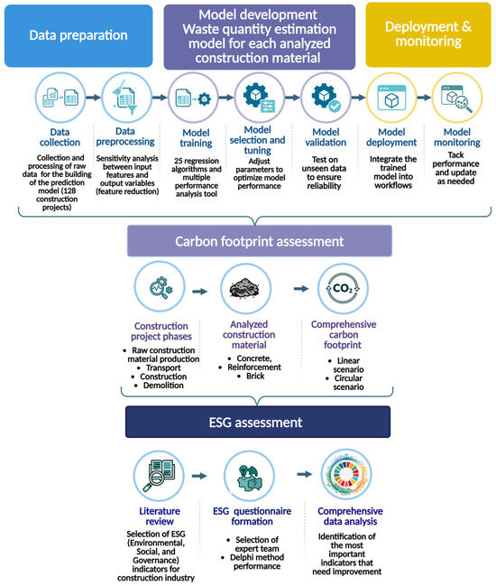
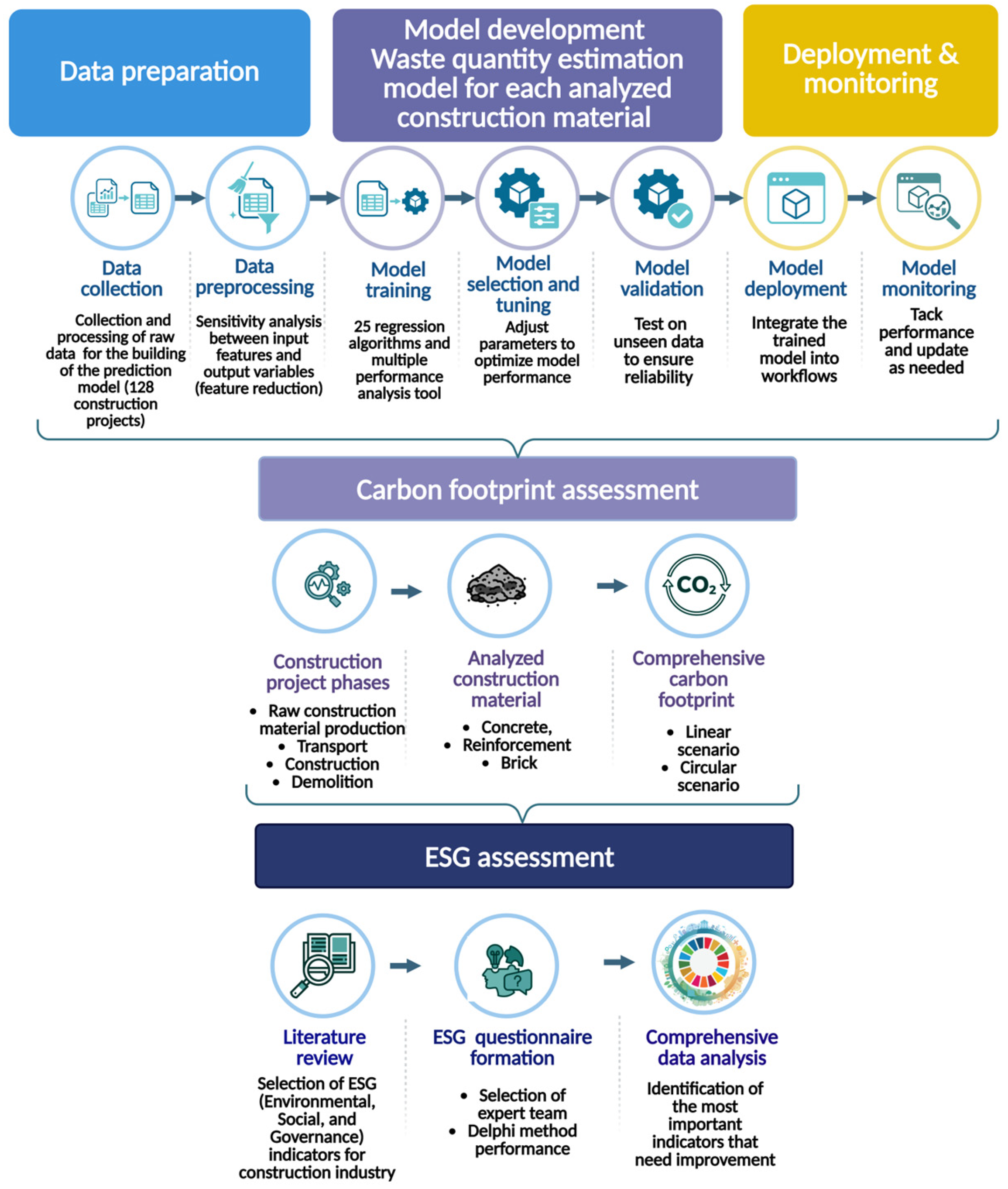
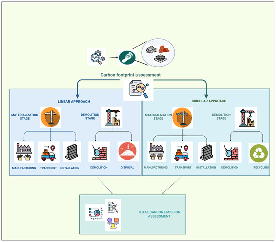
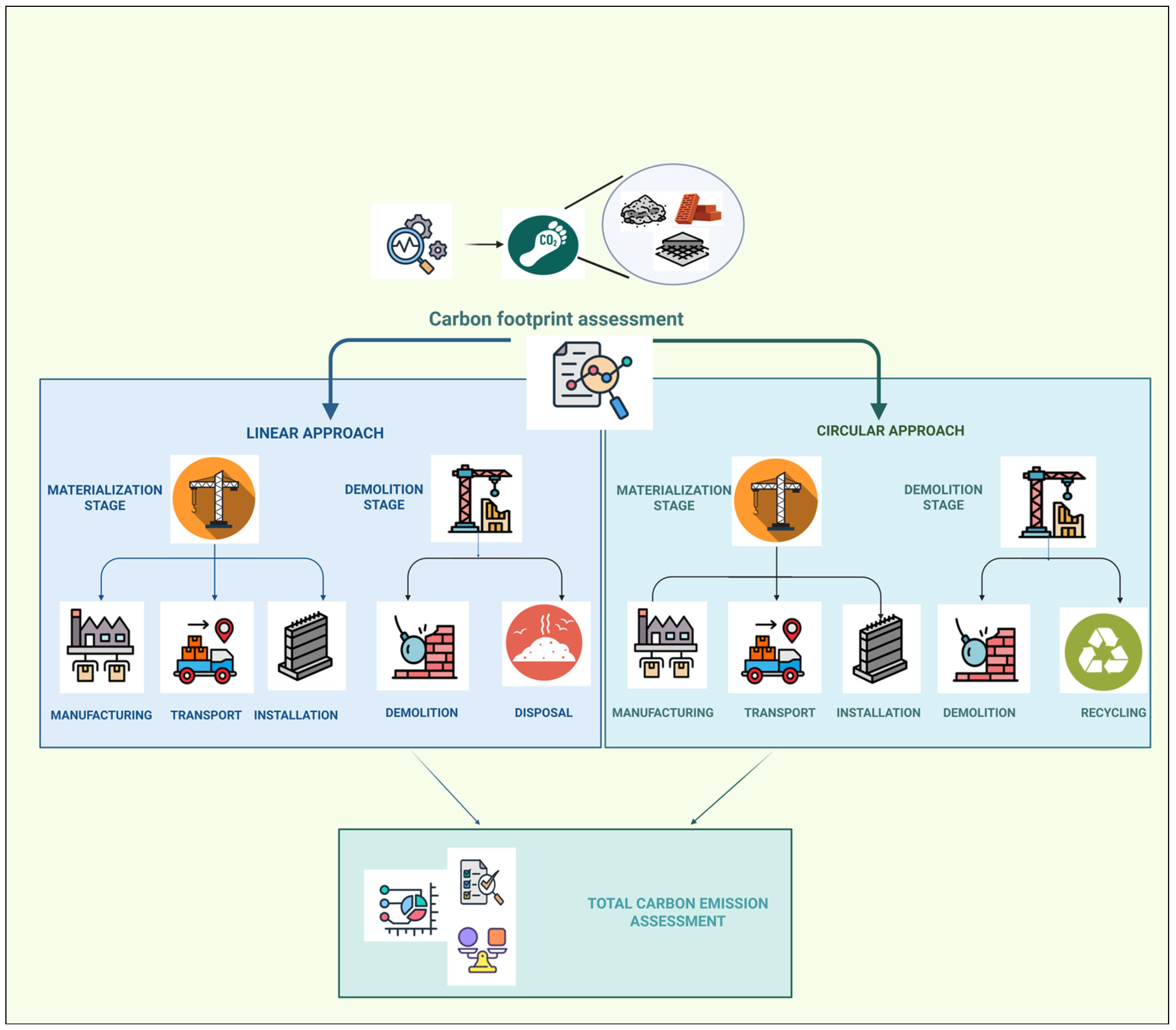


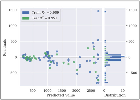
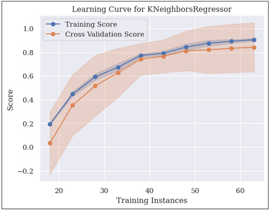
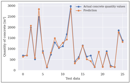
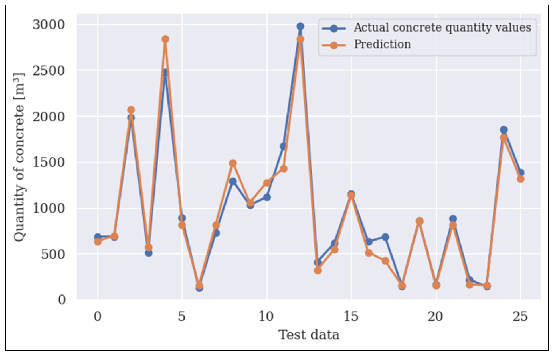
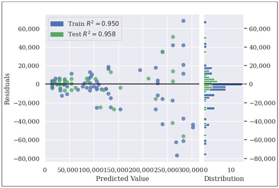
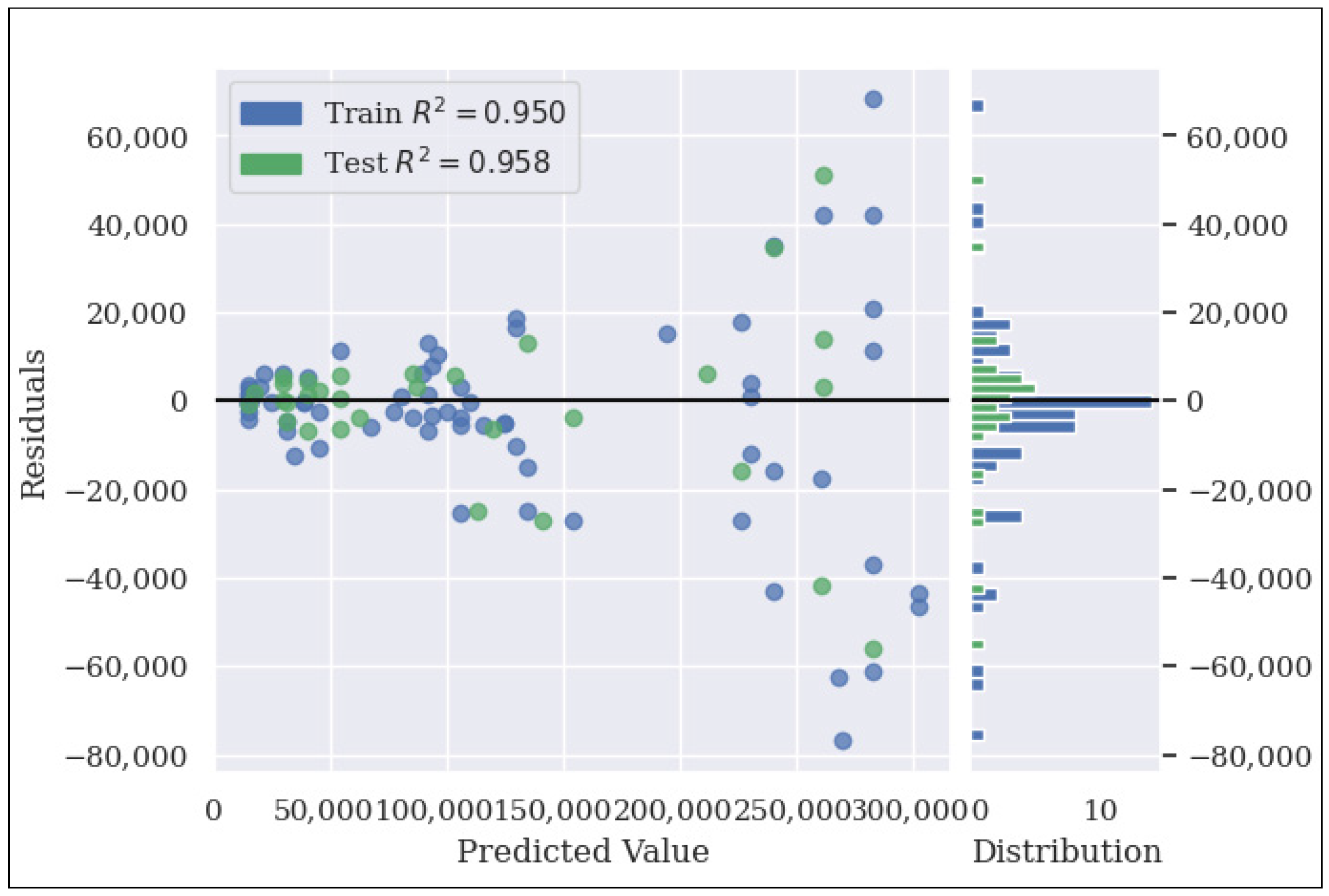
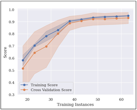
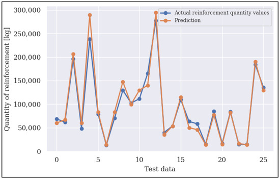
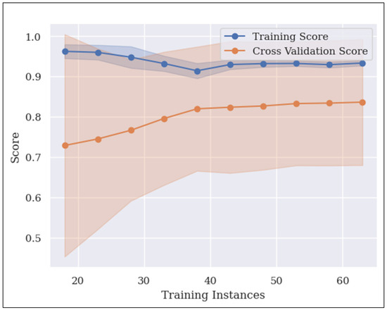
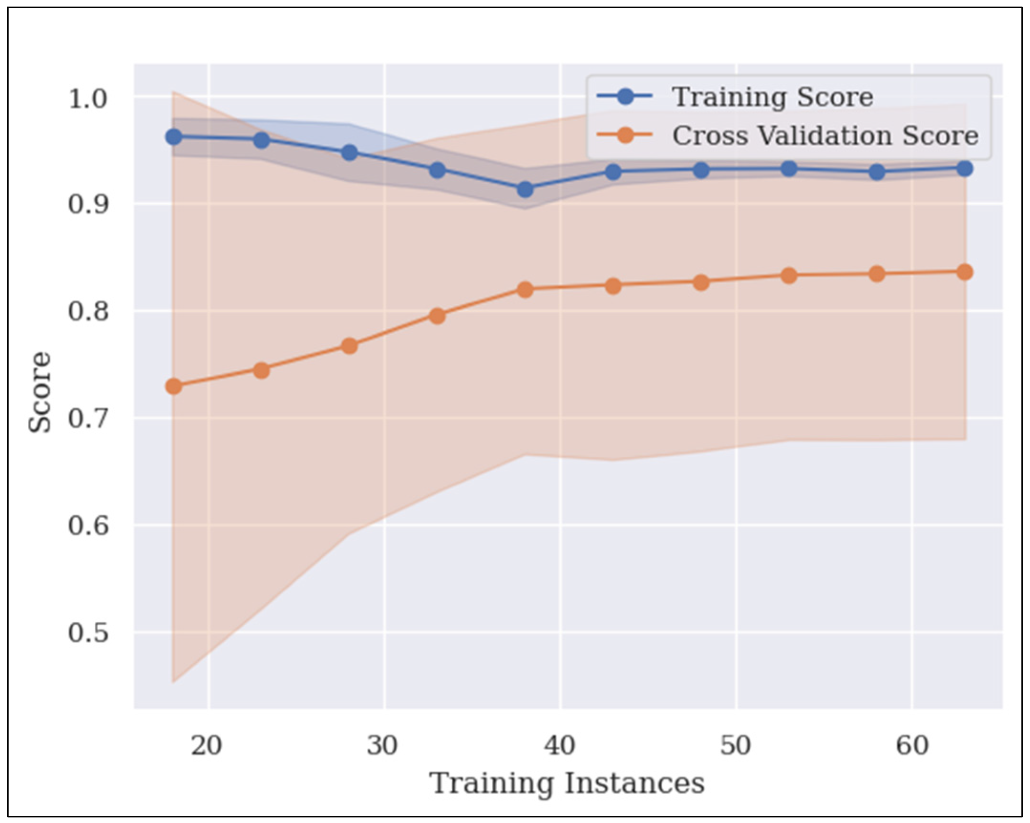
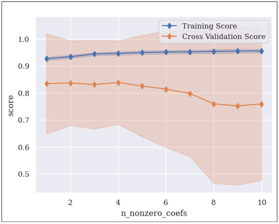
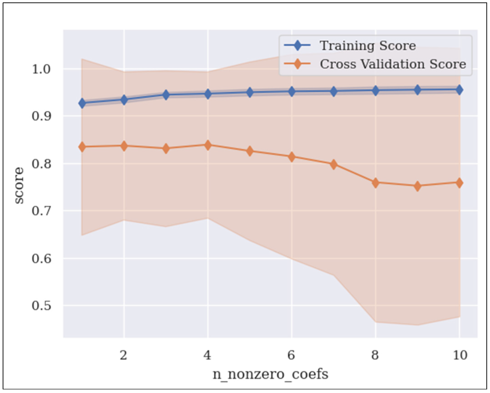
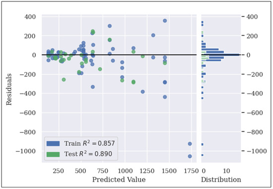
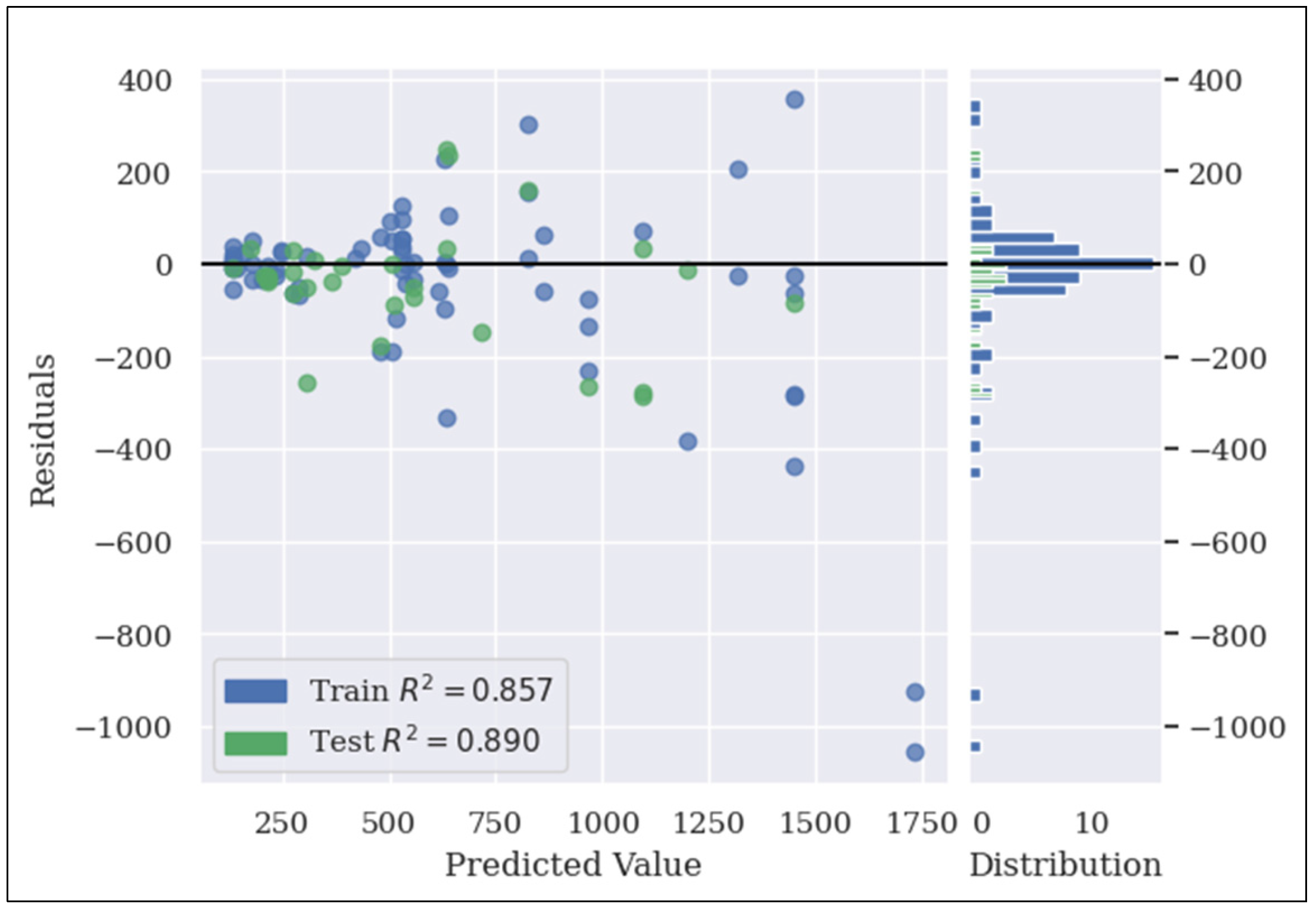
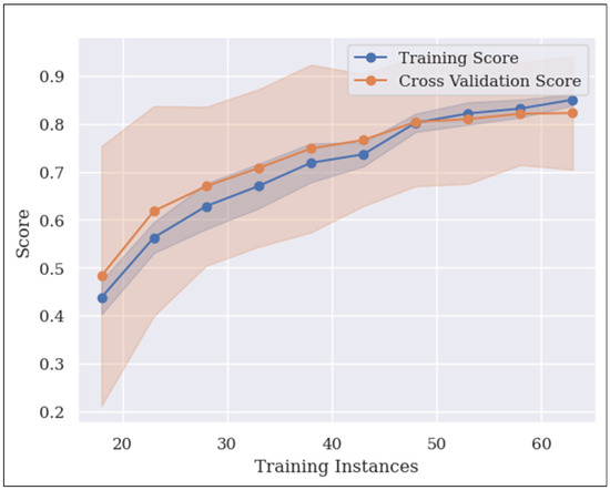
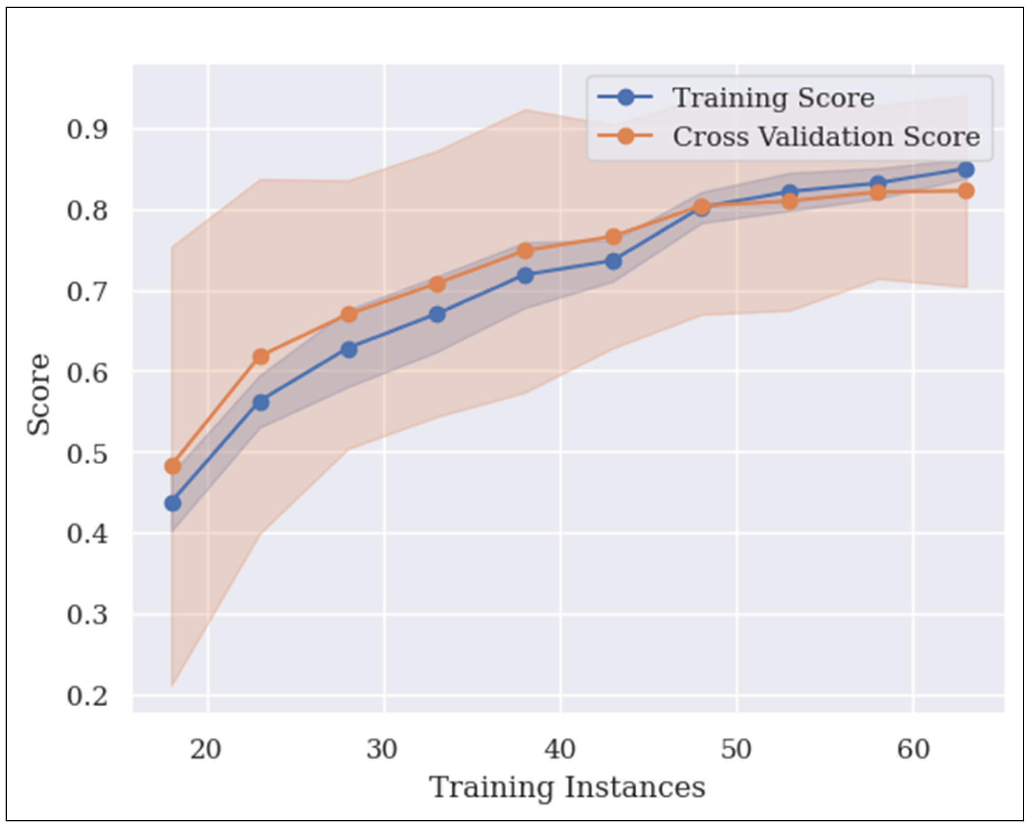
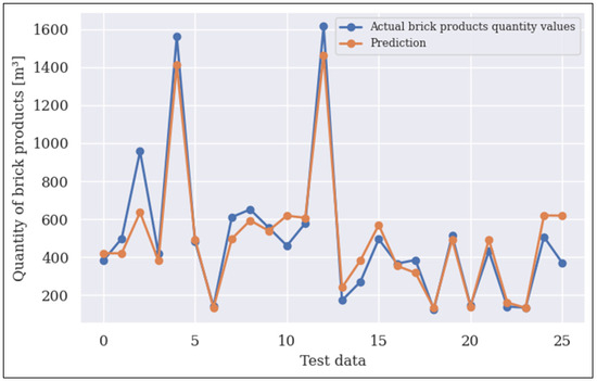
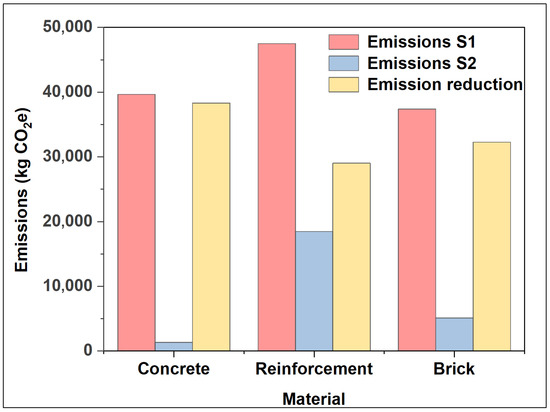
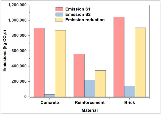
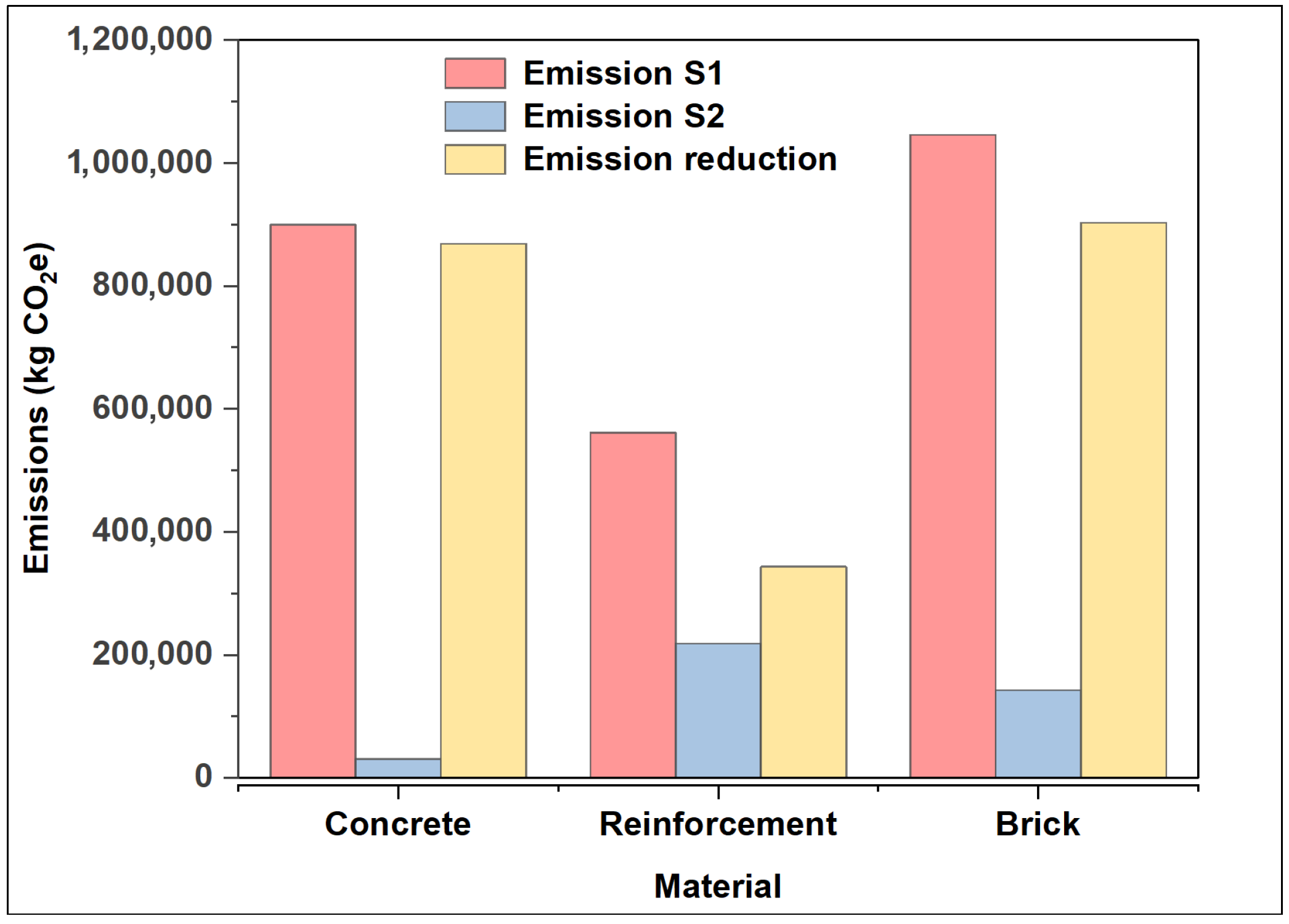
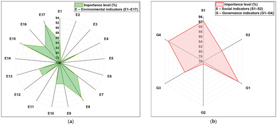
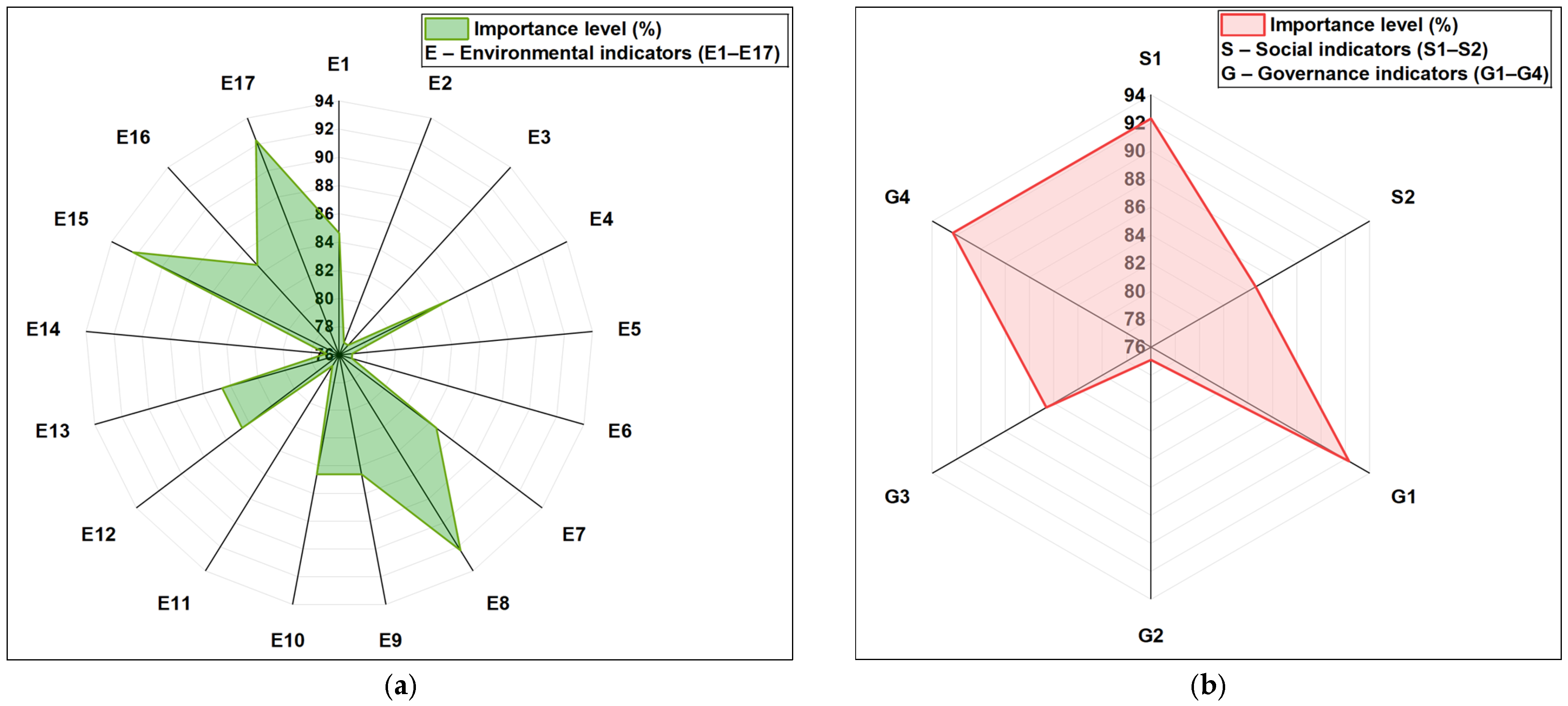
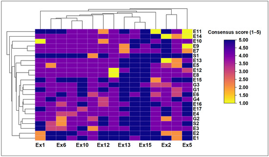
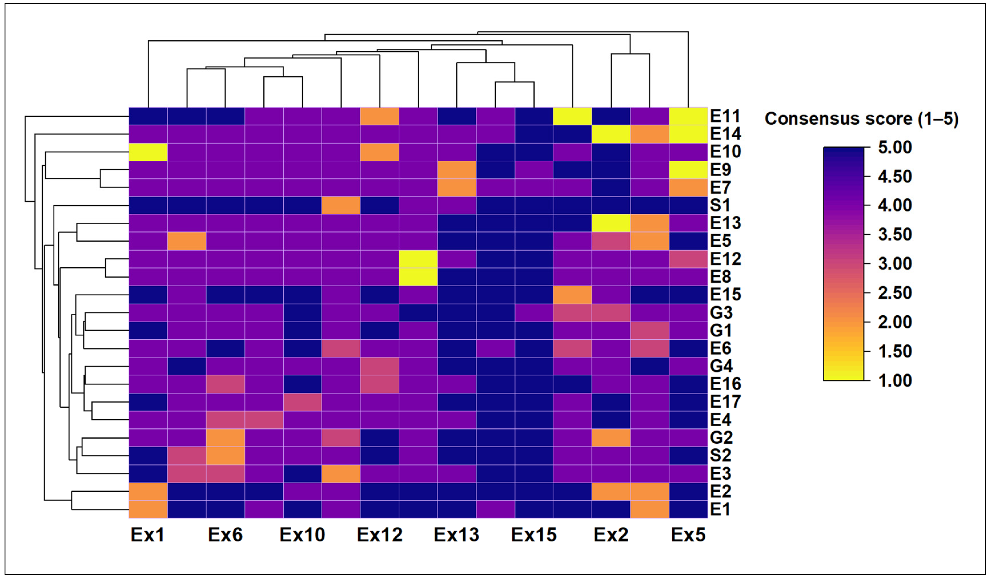

Disclaimer/Publisher’s Note: The statements, opinions and data contained in all publications are solely those of the individual author(s) and contributor(s) and not of MDPI and/or the editor(s). MDPI and/or the editor(s) disclaim responsibility for any injury to people or property resulting from any ideas, methods, instructions or products referred to in the content. |
© 2026 by the authors. Licensee MDPI, Basel, Switzerland. This article is an open access article distributed under the terms and conditions of the Creative Commons Attribution (CC BY) license.