


Abstract
In this work, we present an overview of the recent results, obtained in the framework of the fractional analytic QCD in the space-like (Euclidean) and time-like regions. The Higgs boson decays into a bottom–antibottom pair, and the polarized Bjorken sum rule is considered as an application of the obtained results.
1. Introduction
According to the general principles of (local) quantum field theory (QFT) [1], observables in a space-like region (i.e., in Euclidean space) can only have singularities for negative values of their argument, . However, for large values, these observables are usually represented as power expansions in the running coupling , which has a ghostly singularity, the so-called Landau pole, at . Therefore, to restore the analyticity of the considered expansions, this pole in the strong coupling should be removed.
The strong coupling, , obeys the renormalization group equation
with some boundary condition and the QCD -function, as follows:
where
for f active quark flavors. The first five coefficients, i.e., with , are exactly known [2,3,4,5]. In our present consideration, we will only need .
Note that in Equation (2), we add the first coefficient of the QCD -function to the definition, as is usually done in the analytic version of QCD (see, e.g., Refs. [6,7,8,9,10,11,12]).
So, at the leading order (LO), the next-to-leading order (NLO), and the next-to-next-to-leading order (NNLO), where , and , respectively, we have the following from Equation (1):
i.e., contain poles and other singularities at .
In a time-like region () (i.e., in Minkowski space), the definition of a running coupling is quite difficult. The reason for this problem is that—strictly speaking—the expansion of the perturbation theory (PT) in QCD cannot be defined directly in this region. Since the early days of QCD, much effort has been made to determine the appropriate Minkowski coupling parameter needed to describe important time-like processes, such as -annihilation into hadrons, the formation of quarkonia, and -lepton decays into hadrons. Most attempts (see, for example, [13,14,15]) have relied on the analytical continuation of the strong coupling from the deep Euclidean region—where perturbative QCD calculations can be performed—to Minkowski space, where physical measurements are made. In other developments, analytical expressions for the LO coupling were obtained [16,17] directly in Minkowski space, using an integral transformation from the space-like to time-like modes from the Adler D-function.
Note that, at times, the effective argument of strong coupling reaches a region where perturbation theory becomes of little use. To extend the applicability of perturbation theory, some infrared modifications of the strong coupling are usually used. The most popular modifications are the “freezing” procedure (see, for example, Ref. [18]) and the Shirkov–Solovtsov approach [6,7,8].
The “freezing” of the strong coupling can be done in a hard or a soft way. In the hard case (see [19,20], for example), the strong coupling itself is modified: it is taken to be constant for all values of below a certain threshold, , i.e., if .
In the soft case [18], the argument of the strong coupling is modified. It contains a shift , where is an additional scale (the gluon effective mass) that strongly changes the infrared properties of . For massless-produced quarks, the value of M is usually taken to be the mass of the meson , i.e., . In the case of massive quarks with mass , the value is usually used. In some complicated cases, effective masses with more complicated shapes are used (see, for example, Ref. [21], with examples of masses obtained by solving the Schwinger–Dyson equation, and Refs. [22,23,24,25], where the coupling argument depends on the process under consideration). Moreover, at times, the elimination of the Landau pole leads to additional power-law corrections (see [26,27]).
Hereafter, we will study the analytic coupling. In Refs. [6,7,8,9], an efficient approach was developed to eliminate the Landau singularity without introducing extraneous infrared controllers, such as the gluon effective mass (see, e.g., [18,28,29,30]). (Numerically, couplings with effective mass are very close to the analytic ones (see [31])). This method is based on a dispersion relation that relates the new analytic coupling, , to the spectral function, , obtained in the PT framework. In LO, this gives the following:
The [6,7,8,9] approach follows the corresponding results [32,33] obtained in the framework of quantum electrodynamics. Similarly, the analytical images of a running coupling in Minkowski space are defined using another linear operation:
So, we repeat the following once again: the spectral function in the dispersion relations (5) and (6) is taken directly from PT, and the analytical couplings and are restored using the corresponding dispersion relations. This approach is usually called the minimal approach (MA) (see, e.g., [34]) or the analytical perturbation theory (APT) [6,7,8,9]. (An overview of other similar approaches can be found in [35,36], including approaches that are close to APT [37,38]).
Thus, MA QCD is a very convenient approach that combines the analytical properties of QFT quantities and the results obtained in the framework of perturbative QCD, leading to the appearance of the MA couplings, and , which are close to the usual strong coupling, , in the limit of large values, and completely different from for small values, i.e., for .
A further APT development is the so-called fractional APT (FAPT) [10,11,12], which extends the construction principles described above to the PT series, starting from non-integer powers of the coupling. In the framework of QFT, such series arise for quantities that have nonzero anomalous dimensions. Compact expressions for quantities within the FAPT framework were obtained mainly in LO, but this approach was also used in higher orders, mainly by re-expanding the corresponding couplings in powers of the LO coupling, as well as using some approximations.
In this review, we show the main properties of MA couplings in the FAPT framework, as obtained in Refs. [39,40] using the so-called -expansion. Note that for an ordinary coupling, this expansion is applicable only to large values, i.e., for . However, as shown in [39,40], the situation is quite different with analytic couplings, and this -expansion is applicable to all values of the argument. This is due to the fact that the non-leading expansion corrections vanish not only at , but also at , (The absence of high-order corrections for was also discussed in Refs. [6,7,8,9]). which leads only to nonzero (small) corrections in the region .
Below, we consider the representations for the MA couplings and their (fractional) derivatives obtained in [39,40] (see also [41,42,43]), which are, in principle, valid at any PT order. However, in order to avoid cumbersome formulas while still showing the main features of the approach obtained in [39,40], we restrict our consideration to only the first three PT orders.
Moreover, in this review, we present FAPT applications to the Higgs boson decay into a bottom–antibottom pair and the description of the polarized Bjorken sum rule (BSR). The results shown here were recently obtained in Ref. [40] and Refs. [44,45,46], respectively. In contrast to the formulas, the results for the Higgs boson decay and the polarized BSR will be shown in the first five PT orders, as obtained in [40,44,45,46].
This paper is organized as follows. In Section 2, we first review the basic properties of the usual strong coupling and its -expansion. Section 3 contains fractional derivatives (i.e., -derivatives) of the usual strong coupling, in which -expansions can be represented as some operators acting on the -derivatives of the LO strong coupling. In Section 4 and Section 5, we present the results for the MA couplings. Section 6 contains formulas that are convenient for . In Section 7 and Section 8, we present the integral representations for the MA couplings. Section 9 and Section 10 present applications of this approach to the Higgs boson decay into a bottom–antibottom pair and the Bjorken sum rule, respectively. The conclusion provides final discussions. In addition, we include several appendices, which contain the most complicated expressions.
2. Strong Coupling
As shown in the introduction, the strong coupling obeys the renormalized group Equation (1). When , Equation (1) can be solved iteratively in the form of a -expansion. (The -expansion provides a good approximation for the solution of Equation (2) at (see, for example, [47,48])). In accordance with the reasoning in the introduction, we present the first three terms of the expansion, which can be expressed in the following compact form:
where
The corrections are represented as follows:
As shown in Equations (7) and (9), in any PT order, the coupling contains its dimensional transmutation parameter , which is related to the normalization of as follows:
where in PDG20 [49]. (Notice that the results from PDG20 [49] were used in the considered papers. Now, the new PDG24 [50] presents world average values for the strong coupling: and GeV and GeV).
f-Dependence of the Coupling
The coefficients (3) depend on the number f of active quarks that modify the coupling at thresholds , where an additional quark enters the game, . Here, denotes the mass of the f quark, e.g., GeV and GeV from PDG20 [49]. (Strictly speaking, the quark masses in the scheme depend on and . The -dependence is rather slow and will only be discussed for the decay in Section 9). Thus, the coupling depends on f, and this f-dependence can be taken into account in , i.e., it is that contributes to Equations (1) and (7).
The relationships between and , i.e., the so-called matching conditions between and , are known up to the four-loop order [51,52,53] in the scheme and are usually used for , where these relations have the simplest forms (see, e.g., [54] for a recent review).
Here, we will not consider the f-dependence of and , since we mainly consider the range of small values and, therefore, use from Ref. [55]. Furthermore, since we consider the decay as an application, we will use also the results for , which are also taken from [55]. (The authors of [55] used the PDG20 result, . Now, there is also the PDG21 result, , which contains the same center value. Note that very close numerical relationships between were also obtained by [56] for , extracted by the ZEUS collaboration (see [57])):
We also use , since in the highest orders, values are very similar.
In Figure 1, one can see that the strong couplings become singular at . The values of and are very different (see Equation (11) below): The values of are also shown in Figure 1’s vertical lines.
Figure 1.
The results for and (vertical lines) with . Here, and in the following figures, the values shown in (11) are used.
3. Fractional Derivatives
Following [58,59], we introduce the derivatives (in the -order of PT):
which are very convenient in the case of the analytical QCD (see, e.g., [60]).
The series of derivatives can successfully replace the corresponding series of -degrees. Indeed, each derivative reduces the degree but is accompanied by an additional -function . Thus, each application of a derivative yields an additional , and, thus, it is indeed possible to use a series of derivatives instead of a series of -powers.
In LO, the series of derivatives are exactly the same as . Beyond LO, the relationship between and was established in [59,61], and extended to fractional cases, where is a non-integer , in Ref. [62].
Now, consider the -expansion of . We can raise the -power of the results from (7) and (9) and then restore using the relations between and obtained in [62] (see also Appendix A). This operation is carried out in more detail in Appendix B to [39]. Here, we present only the final results, which have the following form (The expansion (13) is similar to expansions used in Refs. [10,11] for the expansion of in terms of the powers of ).:
where
and are the combinations of the Euler -functions and their derivatives.
The representation (13) of the corrections in terms of -operators is very important. The results for -operators contain the transcendental principle [63,64,65,66]: the corresponding functions () involve Polygamma functions and their products, such as , as well as a larger number of factors, with the same total index k. However, the importance of this property is not yet clear. This allows us to similarly present high-order results for the (-expansion) of analytic couplings.
4. MA Couplings
We first show the LO results, and then go beyond LO, following our results (13) for the ordinary strong coupling obtained in the previous section.
4.1. LO
The LO MA coupling has the following form [10]:
where
is the polylogarithm.
The LO MA coupling in Minkowski space has the following form [11]:
where
4.2. Beyond LO
Following Equations (15) and (17) for the LO analytic couplings, we consider the derivatives of the MA couplings as follows:
By analogy with the ordinary coupling, and using the results from (13) we have the following expressions for the MA couplings and :
where and are given in Equations (15) and (17), respectively, and
and and are given in Equations (13) and (14), respectively.
The relations (15) reflect the fact that the MA procedure (15) and the operation commute. Thus, to obtain (15), we propose that the form (13), used for the usual coupling at high orders, is applicable (exactly in the same way) to the case of the MA coupling.
Space-like case. After some evaluations, we obtained the following expressions without operators:
where
and
We see that the -function and its derivatives have completely canceled out. Note that another form for is given in Appendix B.
So, for the MA analytic couplings, , we have the following expressions:
where
and are given in Equation (13).
Time-like case. Using the results from (13) for the usual coupling, we have the following:
where is given in Equation (17).
This approach allows us to express the high-order corrections in explicit form:
where and are as follows:
and
4.3. The Case
Here, we present only the results for the case :
where and are shown in Equation (19) and
with
Euler constant and
5. The Behaviors of MA Couplings
Here, we show the behaviors of the MA couplings and and compare them.
5.1. Coupling
From Figure 2 and Figure 3, we can see differences between with , which are rather small and have nonzero values around the position . In Figure 2, the values of are shown by vertical lines (as seen in Figure 1).
Figure 2.
The results for and (vertical lines) with .
Figure 3.
The results for () but with the logarithmic scale.
Figure 4 shows the results for and and their differences , which are essentially less than the couplings themselves. From Figure 4, it is clear that for , the asymptotic behaviors of , , and coincide, i.e., the differences and are negligible. Also, Figure 5 shows the differences are essentially less than .
Figure 4.
The results for , and .
Figure 5.
The results for with .
Thus, we can conclude that contrary to the case of the usual coupling, considered in Figure 1, the -expansion of the MA coupling is a very good approximation at any value. Moreover, the differences between and are small. So, the expansions of through the one conducted in Refs. [10,11,12] are very good approximations. Also, the approximation
introduced in [69,70,71,72] and used in [73,74] is very convenient. Indeed, since the corrections are very small, then from Equation (33), one can see that the MA couplings are very similar to the LO ones taken with the corresponding .
5.2. Coupling
This subsection provides graphical results of coupling construction. Figure 6 and Figure 7 show the results for with in usual and logarithmic scales (the last one was chosen to stress the limit ). From Figure 8 and Figure 9, we can see the differences between with , which are rather small and have nonzero values around the position .
Figure 6.
1, 3, and 5 orders of . The vertical lines indicate .
Figure 7.
1, 3, and 5 orders of with a logarithmic scale of s.
Figure 8.
with . The vertical lines indicate .
Figure 9.
with . The vertical line indicates .
So, Figure 6, Figure 7, Figure 8 and Figure 9 show that the difference between and is essentially less than the couplings themselves. From Figure 7, Figure 8 and Figure 9, it is clear that for , the asymptotic behaviors of , , and coincide, i.e., the differences are negligible. Also, Figure 8 and Figure 9 show the differences are essentially less than . We note that the general form of these results coincides with that of the MA couplings , studied in the previous subsection.
5.3. Couplings and
On Figure 10, we see that and are very close to each other for and . The differences between the L0 and NNLO results are nonzero only for .
Figure 10.
The results for and with .
Indeed, the similarity is shown in Figure 11 and Figure 12. In Figure 11, the results for and () are shown in a so-called mirror form, similar to the representation previously introduced in [11]. Figure 12 contains , , and , which are very close to each other but have different limit values when . Moreover, the differences and are almost the same, although the correction to the space-like coupling decreases more rapidly. The direct relation between and gives an interesting picture (see Figure 13). Obviously, we have for any order and the second similar point
for . Higher-order corrections break the identity (40), shifting the second point from . As can be seen in Figure 13, the shift is quite small. As can be seen in Figure 13, the ratio (40) asymptotically approaches 1 when .
Figure 11.
One, three, and five orders of and .
Figure 12.
One and two orders of , , and in Euclidean and Minkowski spaces.
Figure 13.
The relation for . The vertical lines indicate .
In Figure 6, Figure 8, Figure 9 and Figure 13 the values of are shown by vertical lines with color matching in each order. Note that Figure 9 contains only one vertical line since .
Thus, we can conclude that contrary to the case of the usual coupling, the -expansion of the MA coupling is a very good approximation at any value. Moreover, the differences between and are smaller with the increase in order. So, the expansions of through the in Refs. [10,11,12] are very good approximations.
6. MA Coupling : The form Is Convenient for
The results from (26) for analytic coupling are very convenient both at large and small values of values. For , each part—the standard strong coupling and the additional term—has singularities, which are canceled in their sum. So, some numerical applications of the results (26) can be complicated. So, here we present another form, which is very useful at and can be used for any value, except the ranges of very large and very small values. As in the previous section, we will first present the LO results taken from [10] and later extend them beyond LO.
6.1. LO
The LO minimal analytic coupling [6,7,8,9] also has another form [10]:
where Euler functions are
The result from (41) was obtained in Ref. [10], considering the property of the Lerch function, which can be considered a generalization of the polylogarithm (16). The form (41) is very convenient at low L values, i.e., at . Moreover, we can use the relation between and functions:
For , we have the following:
with
and are Bernoulli numbers.
Using the properties of Bernoulli numbers ( is the Kronecker symbol), we have the following for even and for odd values:
Thus, for , we have the following results
with .
6.2. Beyond LO
Now, we consider the derivatives of (minimal) analytic couplings , shown in Equation (20), as in Equation (26), i.e.,
where is given above in (41) with and
where operators are given above in (14).
After some calculations, we have the following:
where, in agreement with (34), we present the following:
with (see Equation (25)) and
Strictly speaking, the series representation (52) for the functions is not a good definition for large r values, and we can replace them with , using the result from (43). However, the results are long and presented in Appendix B.
6.3. The Case
For the case , we immediately have the following:
where is given above in (44) (with the replacement (), and the coefficients can be found in (51) when .
The results from (54) can be expressed in terms of the functions . Using the results in Appendix B and taking the even part () and the odd part () (see Equation (A17)), we have the following:
where
and the functions and are given in Appendix B.
7. Integral Representations for
As already discussed in the introduction, the MA coupling is constructed as follows: The LO spectral function is taken directly from the perturbation theory but the MA coupling itself is built using the correct integration counter. Thus, at LO, the MA coupling obeys Equation (5), as shown in the introduction.
For the -derivative of , i.e., , we have the following equation [62]:
where is the LO spectral function defined in Equation (5) and is the polylogarithmic function presented in (16).
Beyond LO, Equation (59) can be extended in two ways, which will be shown in the following subsections.
7.1. Modification of Spectral Functions
The first possibility of extending the result from (59) beyond LO is related to the modification of the spectral function. The extension is simple and the final result looks as follows:
i.e., it is similar to (59), with the LO spectral function replaced by the -order one :
and (see [37])
with
For the coupling itself, we have the following:
Numerical evaluations of the integrals in (64) can be done following the discussions in Section 4 in Ref. [67].
7.2. Modification of Polylogarithms
Beyond LO, the results from (59) can be extended by using the operators shown in (14). This is the path used in Section 4 and Section 5 to obtain other results.
7.3. Discussions
We considered -expansions of -derivatives of the strong coupling expressed as combinations of operators (14) applied to the LO coupling . Applying the same operators to the -derivatives of the LO MA coupling , we obtained four different representations for the -derivatives of the MA couplings, i.e., , in each i-order of perturbation theory. One form contains a combination of polylogarithms; another contains an expansion of the generalized Euler -function; the third is based on dispersion integrals containing the LO spectral function; the fourth representation is based on the dispersion integral containing the i-order spectral function. All results are presented up to the fifth order of perturbation theory, where the corresponding coefficients of the QCD -function are well-known (see [2,3]).
The high-order corrections are negligible in the and asymptotics and are nonzero in the vicinity of . Thus, they represent only small corrections to the LO MA coupling . This demonstrates the possibility of expanding the high-order couplings via the LO couplings , as was done in Ref. [12], as well as the possibility of various approximations used in [56,69,70,71,72,73,74].
8. Integral Representations for
As mentioned in the introduction, the MA couplings and are constructed as follows: the LO spectral function is taken directly from the perturbation theory but the MA couplings and are obtained using the correct integration contours. Thus, at LO, the MA couplings and obey Equations (5) and (6) presented in the introduction.
For LO, we can take the integral form from [11]
where
Using our approach to obtain high-order terms from LO (69), we can extend the LO integral (69) to the following:
where, obviously, we have the following:
The spectral function has the following form:
where
Explicitly, we have the following:
where and can be obtained from the results in (30) with . They are as follows:
9. Decay
In Ref. [39], we use the polarized Bjorken sum rule [75,76] as an example of the application of the MA coupling , which is a popular object of study in the framework of analytic QCD (see [69,70,73,74,77,78,79,80]). Here, we consider the decay of the Higgs boson into a bottom–antibottom pair, which is also a popular application of the MA coupling (see, e.g., [11] and reviews in Ref. [35]).
The Higgs boson decay into a bottom–antibottom pair can be expressed in QCD by means of the correlator, i.e.,
of two quark scalar (S) currents in terms of the discontinuity of its imaginary part, i.e., , so that the width reads
Direct multi-loop calculations were performed in the Euclidean (space-like) domain for the corresponding Adler function (see Refs. [81,82,83,84,85]). Hence, we write ( and because the additional factor )
where for , the coefficients are
Taking the imagined part, one has the following:
and for [83,84,85,86] (The resummation of the parts can be found in [81] (see also [86]). The results are quite similar to those obtained in the APT case (see [11,35,87]). Such a resummation was not considered in [40] and is, thus, beyond the scope of the present study.)
Here, has the following form (see Appendix C):
where
and are conducted in Equation (A32). For , we have the following:
The normalization constant can be obtained as follows (see, e.g., [35]):
since GeV.
So, we have the following:
where
For , we have the following:
We can express all results through derivatives (see Appendix A):
where
where are given in Appendix A.
For and , we have the following:
Performing the same analysis for the Adler function, we have the following:
where
For , we have the following:
We express all results through derivatives :
where
For and , we have the following:
As discussed earlier in [11], in FAPT, we have the following representation for :
The results for are shown in Figure 14. We see that the FAPT results (99) are lower than those (90) based on conventional PT. This is in full agreement with the arguments given in [35]. But the difference becomes less notable as the PT order increases. Indeed, for LO, the difference is very small, which proves the assumption about the possibility of using the expression for , with , as done in Ref. [11].
Figure 14.
The results for with and 4 in the framework of the usual PT and FAPT.
The results for in the LO approximation using from Equations (87) and (90) are exactly the same and have the following form:
The corresponding results for with from Equation (99) are very similar to the ones in (100). They are as follows:
So, we see good agreement between the results obtained in FAPT and in the framework of the usual PT.
It can be clearly seen that the results of FAPT are also very close to the results [88] obtained in the framework of the now very popular principle of maximum conformality [89,90,91,92,93] (for a recent review, see [94,95]). Indeed, our results are within the band obtained by varying the renormalization scale.
The standard model expectation is [96]
The ratios of the measured events that yield to the standard model expectations are [97] in the ATLAS collaboration and [98] in the SMC collaboration (see also [99]).
Thus, our results—obtained in both approaches, in the standard perturbation theory, and in analytical QCD–are in good agreement with the standard model expectations [96] and the experimental data [97,98].
10. Bjorken Sum Rule
The polarized BSR [100,101] (see also [102,103]) is defined as the difference between the proton and neutron-polarized SFs, integrated over the entire interval x. (The integrals and themselves were studied in [104] but such a study is beyond the scope of this review).
Theoretically, the quantity can be written in the OPE form (see Refs. [105,106]):
where = 1.2762 ± 0.0005 [49] is the nucleon axial charge, is the leading-twist (or twist-two) contribution, and are the higher-twist (HT) contributions. (Below, in our analysis; the so-called elastic contribution will always be excluded.)
Since we plan to consider very small values here, the representation (104) of the HT involves an infinite number of terms. To avoid this, it is preferable to use the so-called “massive” twist-four representation, which includes part of the HT contributions given in (104) (see Refs. [107,108,109]). (Note that Ref. [109] also contains a more complicated form of the “massive” twist-four part. It was included in our previous analysis in [44], but will not be considered here.)
where the values of and were fitted in Refs. [77,79] in the different analytic QCD models. For , the “massive” twist-four representation can be expanded in powers of , and the obtained results will have the form shown on the right-hand side of (104).
In the case of MA QCD, from [79], one can see that in (105), we have the following:
where the statistical (small) and systematic (large) uncertainties are presented.
Up to the k-th order in PT, the twist-two part can be expressed as follows:
where , , and are known from the exact calculations (see, [110] and references therein). The exact value is not known, but it was estimated in Ref. [111].
Converting the coupling powers into its derivatives, we have the following:
where (The resummation of the and parts with renormalon singularities can be found in [112,113,114]. The results based on conventional QCD and APT are quite similar to those obtained in [44,45]. However, such a resummation was not considered in [44,45] and is, thus, beyond the scope of the present study).
and .
In MA QCD, the results from (105) are as follows (some analyses based on other approaches can be found in [112,113,114,115,116,117]):
where the perturbative part takes the same form, however, with analytic coupling (the corresponding expressions are taken from [39])
As already discussed in Section 2, the coefficients depend on the number f of active quarks. So, the coupling is f-dependent and the f-dependence can be taken into the corresponding QCD parameter (see Equation (11)). Since we will mainly consider the region of low , we will use the results for , which we need to construct the analytic coupling for small values.
For the k-th order of PT, we use the results from (11) for taken from the recent Ref. [55], which corresponds to the middle value of the world average [49]. We also use , since in the highest orders, values become very similar. Moreover, since the results for and are taken from the range of values, where the difference between the analytic and usual couplings is small, we will use these values (11) in the analytic QCD case.
For the case involving three active quark flavors (), which is accepted in this paper, we have the following:
i.e., the coefficients in the series of derivatives are slightly smaller.
10.1. Results
The fitting results of experimental data (see [118,119,120,121,122,123,124,125,126,127,128,129,130,131,132,133,134,135,136,137,138,139,140,141,142]) obtained only with statistical uncertainties are presented in Table 1 and shown in Figure 15 and Figure 16. For the fits, we use -independent and and the two-twist part shown in Equations (108) and (111) for regular PT and APT, respectively.
Table 1.
The values of the fit parameters in (110).
Figure 15.
The results for in the first four orders of PT.
Figure 16.
The results for in the first four orders of APT.
As can be seen in Figure 15, with the exception of LO, the results obtained using conventional coupling are very poor. Moreover, the discrepancy in this case increases with the order of PT (see also [69,70,71,72,77,78,79,80] for similar analyses). The LO results describe experimental points relatively well since the value of is quite small compared to other , and disagreement with the data begins at lower values of (see Figure 4 below). Thus, using the “massive” twist-four form (105) does not improve these results, since with , conventional couplings become singular, which leads to large and negative results for the twist-two part (107). So, as the PT order increases, ordinary couplings become singular for ever larger values, while the BSR tends to negative values at increasingly larger values.
In contrast, our results obtained for different APT orders are practically equivalent. The corresponding curves become indistinguishable when approaches 0 and is slightly different everywhere else. As can be seen in Figure 16, the fit quality is pretty high, which is demonstrated by the values of the corresponding (see Table 1).
10.2. Low values
The full picture, however, is more complex than shown in Figure 16. The APT fitting curves become negative (see Figure 17) when we move to very low values of : . So, the high quality of the fits shown in Table 1 results from their good agreement with experimental data at . The picture improves significantly when we compare our results with experimental data for (see Figure 18 and Ref. [44]).
Figure 17.
The same as in Figure 16 but for .
Figure 18.
The results for using the first four orders of APT, from fits of experimental data with .
Figure 18 also shows contributions from conventional PT at the first two orders: the LO and NLO predictions, which have no resemblance to the experimental data. As mentioned above, higher orders lead to even worse agreement, and are, therefore, not shown. The purple curve emphasizes the key role of the twist-four contribution (see also [72,143,144]) and the discussions therein). Excluding this contribution, the value of is about 0.16, which is very far from the experimental data.
At , we also see good agreement with the phenomenological models: LFHQCD [145] and the correct IR limit of the Burkert–Ioffe model [146,147]. For larger values of , our results are lower than the results of the phenomenological models, and for —below the experimental data.
Nevertheless, even in this case, where very good agreement with experimental data with is demonstrated, our results for take negative unphysical values when . The reason for this phenomenon can be seen by considering photoproduction within APT, which is the topic of the next subsection.
10.3. Photoproduction
To understand the problem demonstrated above, , we consider the photoproduction case. In the k-th order of MA QCD,
and, so, we have
The finiteness of the cross-section in the real photon limit leads to [107]
For , we have the following:
shown in (106) and in Table 1.
So, as can be seen from Table 1, the finiteness of the cross-section in the real photon limit is violated in our approaches. (Note that the results for were obtained by only taking into statistical uncertainties. When adding systematic uncertainties, the results for and are completely consistent with each other, but the predictive power of such an analysis is small). This violation leads to negative values of . Note that this violation is less for experimental datasets with , where the obtained values for are essentially less than those obtained in the case of experimental data with . Smaller values of lead to negative values of , when (see Figure 4).
10.4. Gerasimov–Drell–Hearn and Burkhardt–Cottingham Sum Rules
Now, we plan to improve this analysis by involving the results from (110) at low values and taking into account the “massive” twist-six term, similar to the twist-four shown in Equation (105).
Moreover, we take into account the GDH and BC sum rules, which lead to (see [104,107,108,109,148,149])
where and are proton and neutron magnetic moments, respectively, and = 0.938 GeV is a nucleon mass. Note that the value of G is small.
In agreement with the definition (12), we have the following:
Then, as , for any n value, we obtain the following:
but very slowly, so that the derivative behaves as follows:
Thus, after applying the derivative for , every term in becomes divergent as . To produce finiteness at for the l.h.s. of (117), we can assume the relation between twist-two and twist-four terms, which leads to the appearance of a new contribution:
which can be done to remain regular as .
The form (121) suggests the following idea about a modification of in (110):
where we add the “massive” twist-six term and introduce different masses in both higher-twist terms and into the modification factor .
The finiteness of the cross-section in the real photon limit now leads to the following [107,108]:
and, thus, we have the following:
Using (i.e., ), we have the following:
Using the results from (123) and (126) together, we have the following:
Since the value of G is small, so and .
The fitting results of theoretical predictions based on Equation (122), with and , as outlined in (127), are presented in Table 2 and Figure 19 and Figure 20.
Table 2.
The values of the fit parameters.
Figure 19.
The results for (122) in the first four orders of APT.
Figure 20.
As in Figure 19 but for .
As one can see in Table 2, the obtained results for are different if we take the full dataset and the limited one with . However, the difference is significantly less than in Table 1. Moreover, the results obtained in the fits using the full dataset and shown in Table 1 and Table 2 are quite similar.
We also see some similarities between the results shown in Figure 16 and Figure 19. The difference appears only at small values, as can be seen in Figure 17 and Figure 20.
Figure 20 also shows that the results of fitting the full set of experimental data are in better agreement with the data at , as expected, since these data are involved in the analyses of the full set of experimental data.
11. Conclusions
In this paper, we presented an overview of fractional analytic QCD and its application to the Higgs boson decay into a bottom–antibottom pair and for the polarized Bjorken sum rule.
We considered -expansions of -derivatives of the strong coupling expressed as combinations of operators (14) applied to the LO coupling . Applying the same operators to the -derivatives of the LO MA coupling , we obtained four different representations for the -derivatives of the MA couplings, i.e., , in each i-order of perturbation theory: one form contains a combination of polylogarithms; another contains an expansion of the generalized Euler -function; the third is based on dispersion integrals containing the LO spectral function; and the fourth representation is based on the dispersion integral containing the i-order spectral function. All results are presented up to the fifth order of the perturbation theory, where the corresponding coefficients of the QCD -function are well known (see [2,3]).
The high-order corrections are negligible in the and asymptotics and are nonzero in the vicinity of the point . Thus, in fact, they are really only small corrections to the LO MA coupling . This proves the possibility of expansions of high-order couplings via the LO couplings , as done in Ref. [12], as well as the possibility of various approximations used in [56,69,70,71,72,73,74].
As can be seen, all our results (up to the fifth order of perturbation theory) maintain a compact form and do not contain complicated special functions, such as the Lambert W-function [154,155,156], which already appears at the two-loop order as an exact solution to the usual coupling, and was used to evaluate MA couplings in [157,158].
Applying the same operators to the -derivatives of the LO MA coupling , we obtained two different representations (see Equations (29) and (71)) for the -derivatives of the MA couplings (i.e., introduced for time-like processes) in each i-order of perturbation theory: one form contains a combination of trigonometric functions, and the other is based on dispersion integrals containing the i-order spectral function. All results are presented up to the fifth order of perturbation theory.
As in the case of [39] applied in the Euclidean space, high-order corrections for are negligible in the and limits and are nonzero in the vicinity of the point . Thus, there are only small corrections to the LO MA coupling . In particular, this proves the possibility of expansions of high-order couplings via the LO couplings , as done in Ref. [12].
As an example, we examined the Higgs boson decay into a pair and the obtained results are in good agreement with the standard model expectations [96] and with the experimental data [97,98]. Moreover, our results are also in good agreement with studies based on the principle maximum conformality [89,90,91,92,93].
As a second application, we considered the Bjorken sum rule in the framework of MA and perturbative QCD, and obtained results similar to those obtained in previous studies [44,69,70,72,77,79] for the first four orders of PT. The results based on conventional PT do not agree with the experimental data. For some values, the PT results were negative, since the high-order corrections were large and entered the twist-two term with a minus sign. APT in the minimal version led to good agreement with experimental data when we used the “massive” version (110) for the twist-four contributions.
Examining low behavior, we found that there was a disagreement between the results obtained in the fits and application of MA QCD to photoproduction. The fit results, when extended to low values, led to negative values for the Bjorken sum rule : . This was contrary to the finiteness of the cross-section in the real photon limit leading to . Note that fits of experimental data at low values (we used ) led to less magnitudes of negative values for (see Table 1 and Table 2).
To solve the problem, we considered low modifications of the OPE formula for . Carefully considering one of them, Equation (122), we find good agreement with full sets of experimental data for the Bjorken sum rule and with its limit, i.e., with photoproduction. We also see good agreement with phenomenological models [104,146,147,148,149], especially with LFHQCD [145].
Author Contributions
Investigation, I.R.G., N.A.G., A.V.K., O.V.T., D.A.V. and I.A.Z., Writing—original draft, I.R.G., N.A.G., A.V.K., O.V.T., D.A.V. and I.A.Z. All authors have read and agreed to the published version of the manuscript.
Funding
N.A.G., A.V.K. and D.A.V. was funded by the Foundation for the Advancement of Theoretical Physics and Mathematics “BASIS”, grant number 22-1-1-30-1; I.A.Z. was funded by the Directorate of Postgraduate Studies of the Technical University of Federico Santa Maria.
Data Availability Statement
Not applicable.
Acknowledgments
We are grateful to Gorazd Cvetic for initiating these studies and collaborating at the initial stage and Alexander Nesterenko for the information about the 5-loop spectral function calculated in his paper [68]. We are also grateful to Alexandre P. Deur for information about the new experimental data in Ref. [118]. The authors thank Konstantin Chetyrkin, Andrei Kataev, and Sergey Mikhailov for the careful discussions.
Conflicts of Interest
The authors declare no conflicts of interest.
Appendix A. Details of the Evaluation of the Fractional Derivatives
Taking the results (7) of the coupling , we have the following results for the -expansion of its -powers:
where is defined in Equation (8), and
which is consistent with the expansions made in Refs. [10,11].
The -derivative is related to the powers as follows:
where (see [62])
with
and
with the Euler constant and Euler function . The expression for with arbitrary k can be found in [62].
After some calculations, we have the following:
where
and
and is given in Equation (13) and
with
where are defined in Equation (A6).
It is convenient to introduce the operators (13), which is given by . In this case, we proceed to the results (13) and (14) of the main text.
It is convenient to express through . Considering Ref. [62], we have the following:
where
where
and
For arbitrary values, are expressed through Polygamma-functions (see (A6)). In the case of integer , we have the following:
Appendix B. Alternative Form for the Couplings
Using the series representation (52), the functions in (51) are not well-defined for large r values, and by , and we will replace them using the result from (43) as
Moreover, here, we use the following:
Appendix C.
Here, we present an evaluation of , which has the following form:
where
Evaluating the integral in (A25), we have the following results (see, e.g., Refs. [11,159]):
where
and
with
The result for can be rewritten as follows:
where
References
- Bogolyubov, N.N.; Shirkov, D.V. Introduction to the theory of quantized fields. Intersci. Monogr. Phys. Astron. 1959, 3, 1–720. [Google Scholar] [CrossRef] [Scilit]
- Baikov, P.A.; Chetyrkin, K.G.; Kühn, J.H. Five-Loop Running of the QCD coupling constant. Phys. Rev. Lett. 2017, 118, 082002. [Google Scholar] [CrossRef] [Scilit]
- Herzog, F.; Ruijl, B.; Ueda, T.; Vermaseren, J.A.M.; Vogt, A. The five-loop beta function of Yang-Mills theory with fermions. J. High Energy Phys. 2017, 2017, 90. [Google Scholar] [CrossRef] [Scilit]
- Luthe, T.; Maier, A.; Marquard, P.; Schroder, Y. The five-loop Beta function for a general gauge group and anomalous dimensions beyond Feynman gauge. J. High Energy Phys. 2017, 10, 166. [Google Scholar] [CrossRef] [Scilit]
- Chetyrkin, K.G.; Falcioni, G.; Herzog, F.; Vermaseren, J.A.M. Five-loop renormalisation of QCD in covariant gauges. J. High Energy Phys. 2017, 10, 179. [Google Scholar] [CrossRef] [Scilit]
- Shirkov, D.V.; Solovtsov, I.L. Analytic model for the QCD running coupling with universal αs(0) value. Phys. Rev. Lett. 1997, 79, 1209–1212. [Google Scholar] [CrossRef] [Scilit]
- Shirkov, D.V. Analytic perturbation theory for QCD observables. Theor. Math. Phys. 2001, 127, 409–423. [Google Scholar] [CrossRef] [Scilit]
- Shirkov, D.V. Analytic perturbation theory in analyzing some QCD observables. Eur. Phys. J. C 2001, 22, 331–340. [Google Scholar] [CrossRef] [Scilit]
- Milton, K.A.; Solovtsov, I.L.; Solovtsova, O.P. Analytic perturbation theory and inclusive tau decay. Phys. Lett. B 1997, 415, 104–110. [Google Scholar] [CrossRef] [Scilit]
- Bakulev, A.P.; Mikhailov, S.V.; Stefanis, N.G. QCD analytic perturbation theory: From integer powers to any power of the running coupling. Phys. Rev. D 2005, 72, 074014, Erratum in Phys. Rev. D 2005, 72, 119908. [Google Scholar] [CrossRef] [Scilit]
- Bakulev, A.P.; Mikhailov, S.V.; Stefanis, N.G. Fractional Analytic Perturbation Theory in Minkowski space and application to Higgs boson decay into a b anti-b pair. Phys. Rev. D 2007, 75, 056005, Erratum in Phys. Rev. D 2008, 77, 079901. [Google Scholar] [CrossRef] [Scilit]
- Bakulev, A.P.; Mikhailov, S.V.; Stefanis, N.G. Higher-order QCD perturbation theory in different schemes: From FOPT to CIPT to FAPT. J. High Energy Phys. 2010, 2010, 85. [Google Scholar] [CrossRef] [Scilit]
- Pennington, M.R.; Ross, G.G. Perturbative QCD for Timelike Processes: What Is the Best Expansion Parameter? Phys. Lett. B 1981, 102, 167–171. [Google Scholar] [CrossRef] [Scilit]
- Pennington, M.R.; Roberts, R.G.; Ross, G.G. How to Continue the Predictions of Perturbative QCD From the Space-Like Region Where They Are Derived to the Time-Like Regime Where Experiments Are Performed. Nucl. Phys. B 1984, 242, 69–80. [Google Scholar] [CrossRef] [Scilit]
- Marshall, R. A Determination of the Strong Coupling Constant α−s From e+e− Total Cross-section Data. Z. Phys. C 1989, 43, 595. [Google Scholar] [CrossRef] [Scilit]
- Krasnikov, N.V.; Pivovarov, A.A. The influence of the analytical continuation effects on the value of the qcd scale parameter lambda extracted from the data on charmonium and upsilon hadron decays. Phys. Lett. B 1982, 116, 168–170. [Google Scholar] [CrossRef] [Scilit]
- Radyushkin, A.V. Optimized Λ-Parametrization for the QCD Running Coupling Constant in Space-Like and Time-Like Regions. JINR Rapid Commun. 1996, 78, 9, [hep-ph/9907128]. [Google Scholar]
- Badelek, B.; Kwiecinski, J.; Stasto, A. A Model for F(L) and R = F(L) / F(T) at low x and low Q2. Z. Phys. C 1997, 74, 297–306. [Google Scholar]
- Nikolaev, N.N.; Zakharov, B.G. Color transparency and scaling properties of nuclear shadowing in deep inelastic scattering. Z. Phys. C 1991, 49, 607–618. [Google Scholar] [CrossRef] [Scilit]
- Nikolaev, N.; Zakharov, B.G. Pomeron structure function and diffraction dissociation of virtual photons in perturbative QCD. Z. Phys. C 1992, 53, 331–346. [Google Scholar] [CrossRef] [Scilit]
- Deur, A.; Brodsky, S.J.; de Teramond, G.F. The QCD Running Coupling. Nucl. Phys. 2016, 90, 1. [Google Scholar] [CrossRef] [Scilit]
- Becher, T.; Neubert, M. Drell-Yan Production at Small qT, Transverse Parton Distributions and the Collinear Anomaly. Eur. Phys. J. C 2011, 71, 1665. [Google Scholar] [CrossRef] [Scilit]
- Becher, T.; Neubert, M.; Wilhelm, D. Electroweak Gauge-Boson Production at Small qT: Infrared Safety from the Collinear Anomaly. J. High Energy Phys. 2012, 2012, 124. [Google Scholar] [CrossRef] [Scilit]
- Becher, T.; Neubert, M.; Wilhelm, D. Higgs-Boson Production at Small Transverse Momentum. J. High Energy Phys. 2013, 2013, 110. [Google Scholar] [CrossRef] [Scilit]
- Catani, S.; Grazzini, M. Higgs Boson Production at Hadron Colliders: Hard-Collinear Coefficients at the NNLO. Eur. Phys. J. C 2012, 72, 2013. [Google Scholar] [CrossRef] [Scilit]
- Becher, T.; Neubert, M.; Pecjak, B.D. Factorization and Momentum-Space Resummation in Deep-Inelastic Scattering. J. High Energy Phys. 2007, 01, 76. [Google Scholar] [CrossRef] [Scilit]
- Catani, S.; Mangano, M.L.; Nason, P.; Trentadue, L. The Resummation of soft gluons in hadronic collisions. Nucl. Phys. B 1996, 478, 273–310. [Google Scholar] [CrossRef] [Scilit]
- Ducati, M.B.G.; Halzen, F.; Natale, A.A. Diffraction and the gluon mass. Phys. Rev. D 1993, 48, 2324–2328. [Google Scholar] [CrossRef] [Scilit]
- Mattingly, A.C.; Stevenson, P.M. QCD perturbation theory at low-energies. Phys. Rev. Lett. 1992, 69, 1320–1323. [Google Scholar] [CrossRef] [Scilit]
- Mattingly, A.C.; Stevenson, P.M. Optimization of R(e+ e−) and ‘freezing’ of the QCD couplant at low-energies. Phys. Rev. D 1994, 49, 437–450. [Google Scholar] [CrossRef] [Scilit]
- Kotikov, A.V.; Lipatov, A.V.; Zotov, N.P. The Longitudinal structure function F(L): Perturbative QCD and k(T) factorization versus experimental data at fixed W. J. Exp. Theor. Phys. 2005, 101, 811–816. [Google Scholar] [CrossRef] [Scilit]
- Bogolyubov, N.N.; Logunov, A.A.; Shirkov, D.V. The method of dispersion relations and perturbation theory. Sov. Phys. JETP 1960, 10, 574–581. [Google Scholar]
- Redmond, P.J. Elimination of Ghosts in Propagators. Phys. Rev. 1958, 112, 1404. [Google Scholar] [CrossRef] [Scilit]
- Cvetic, G.; Valenzuela, C. Analytic QCD: A Short review. Braz. J. Phys. 2008, 38, 371–380. [Google Scholar]
- Bakulev, A.P. Global Fractional Analytic Perturbation Theory in QCD with Selected Applications. Phys. Part. Nucl. 2009, 40, 715–756. [Google Scholar] [CrossRef] [Scilit]
- Stefanis, N.G. Taming Landau singularities in QCD perturbation theory: The Analytic approach. Phys. Part. Nucl. 2013, 44, 494–509. [Google Scholar] [CrossRef] [Scilit]
- Nesterenko, A.V. Analytic invariant charge in QCD. Int. J. Mod. Phys. A 2003, 18, 5475–5520. [Google Scholar] [CrossRef] [Scilit]
- Nesterenko, A.V.; Papavassiliou, J. The Massive analytic invariant charge in QCD. Phys. Rev. D 2005, 71, 016009. [Google Scholar] [CrossRef] [Scilit]
- Kotikov, A.V.; Zemlyakov, I.A. Fractional analytic QCD beyond leading order. J. Phys. G 2023, 50, 015001. [Google Scholar] [CrossRef] [Scilit]
- Kotikov, A.V.; Zemlyakov, I.A. Fractional analytic QCD beyond leading order in the timelike region. Phys. Rev. D 2023, 107, 094034. [Google Scholar] [CrossRef] [Scilit]
- Kotikov, A.V.; Zemlyakov, I.A. About Fractional Analytic QCD beyond Leading Order. arXiv 2022, arXiv:2207.01330. [Google Scholar]
- Kotikov, A.V.; Zemlyakov, I.A. About Fractional Analytic QCD. Phys. Part. Nucl. 2023, 54, 942–947. [Google Scholar] [CrossRef] [Scilit]
- Kotikov, A.V.; Zemlyakov, I.A. On Fractional Analytic QCD. Phys. Part. Nucl. 2024, 55, 863–867. [Google Scholar] [CrossRef] [Scilit]
- Gabdrakhmanov, I.R.; Gramotkov, N.A.; Kotikov, A.V.; Volkova, D.A.; Zemlyakov, I.A. Bjorken sum rule with analytic coupling at low Q2 values. JETP Lett. 2023, 118, 478–482. [Google Scholar] [CrossRef] [Scilit]
- Gabdrakhmanov, I.R.; Gramotkov, N.A.; Kotikov, A.V.; Teryaev, O.V.; Volkova, D.A.; Zemlyakov, I.A. Bjorken sum rule with analytic coupling. arXiv 2024, arXiv:2404.01873. [Google Scholar] [CrossRef] [Scilit]
- Gabdrakhmanov, I.R.; Gramotkov, N.A.; Kotikov, A.V.; Teryaev, O.V.; Volkova, D.A.; Zemlyakov, I.A. On Bjorken sum rule with analytic coupling. arXiv 2024, arXiv:2406.20000. [Google Scholar] [CrossRef] [Scilit]
- Shaikhatdenov, B.G.; Kotikov, A.V.; Krivokhizhin, V.G.; Parente, G. QCD coupling constant at NNLO from DIS data. Phys. Rev. D 2010, 81, 034008, Erratum in Phys. Rev. D 2010, 81, 079904. [Google Scholar] [CrossRef] [Scilit]
- Krivokhizhin, V.G.; Kotikov, A.V. A systematic study of QCD coupling constant from deep-inelastic measurements. Phys. Atom. Nucl. 2005, 68, 1873–1903. [Google Scholar] [CrossRef] [Scilit]
- Particle Data Group; Zyla, P.; Barnett, R.M.; Beringer, J.; Dahl, O.; Dwyer, D.A.; Groom, D.E.; Lin, C.J.; Lugovsky, K.S.; Pianori, E.; et al. Review of Particle Physics. Prog. Theor. Exp. Phys. 2020, 8, 083C01. [Google Scholar] [CrossRef] [Scilit]
- Navas, S.; Amsler, C.; Gutsche, T.; Hanhart, C.; Hernández-Rey, J.J.; Lourenço, C.; Masoni, A.; Mikhasenko, M.; Mitchell, R.E.; Patrignani, C.; et al. Review of particle physics. Phys. Rev. D 2024, 110, 030001. [Google Scholar] [CrossRef] [Scilit]
- Chetyrkin, K.G.; Kuhn, J.H.; Sturm, C. QCD decoupling at four loops. Nucl. Phys. B 2006, 744, 121–135. [Google Scholar] [CrossRef] [Scilit]
- Schroder, Y.; Steinhauser, M. Four-loop decoupling relations for the strong coupling. J. High Energy Phys. 2006, 2006, 51. [Google Scholar] [CrossRef] [Scilit]
- Kniehl, B.A.; Kotikov, A.V.; Onishchenko, A.I.; Veretin, O.L. Strong-coupling constant with flavor thresholds at five loops in the anti-MS scheme. Phys. Rev. Lett. 2006, 97, 042001. [Google Scholar] [CrossRef] [Scilit] [PubMed]
- d’Enterria, D.; Rojo, J.; Brambilla, N.; Reichelt, D.; Jamin, M.; Maltman, K.; Sint, S.; Teca, D.; Britzger, D.; Kronfeld, A.S.; et al. The strong coupling constant: State of the art and the decade ahead. arXiv 2022, arXiv:2203.08271. [Google Scholar] [CrossRef] [Scilit]
- Chen, H.M.; Liu, L.M.; Wang, J.T.; Waqas, M.; Peng, G.X. Matching-invariant running of quark masses in quantum chromodynamics. Int. J. Mod. Phys. E 2022, 31, 2250016. [Google Scholar] [CrossRef] [Scilit]
- Illarionov, A.Y.; Kotikov, A.V.; Bermudez, G.P. Small x behavior of parton distributions. A Study of higher twist effects. Phys. Part. Nucl. 2008, 39, 307–347. [Google Scholar] [CrossRef] [Scilit]
- Zeus Collaboration; Chekanov, S. Measurement of the neutral current cross section and structure function for deep inelastic scattering at HERA. Eur. Phys. J. C-Part. Fields 2001, 21, 443–471. [Google Scholar] [CrossRef] [Scilit]
- Cvetic, G.; Valenzuela, C. An Approach for evaluation of observables in analytic versions of QCD. J. Phys. G 2006, 32, L27. [Google Scholar] [CrossRef] [Scilit]
- Cvetic, G.; Valenzuela, C. Various versions of analytic QCD and skeleton-motivated evaluation of observables. Phys. Rev. D 2006, 74, 114030, Erratum in Phys. Rev. D 2011, 84, 019902. [Google Scholar] [CrossRef] [Scilit]
- Kotikov, A.V.; Zemlyakov, I.A. About Derivatives in Analytic QCD. JETP Lett. 2022, 115, 565–569. [Google Scholar] [CrossRef] [Scilit]
- Cvetic, G.; Kogerler, R.; Valenzuela, C. Reconciling the analytic QCD with the ITEP operator product expansion philosophy. Phys. Rev. D 2010, 82, 114004. [Google Scholar] [CrossRef] [Scilit]
- Cvetič, G.; Kotikov, A.V. Analogs of noninteger powers in general analytic QCD. J. Phys. G 2012, 39, 065005. [Google Scholar] [CrossRef] [Scilit]
- Kotikov, A.V.; Lipatov, L.N. NLO corrections to the BFKL equation in QCD and in supersymmetric gauge theories. Nucl. Phys. B 2000, 582, 19–43. [Google Scholar] [CrossRef] [Scilit]
- Kotikov, A.V.; Lipatov, L.N. DGLAP and BFKL equations in the N = 4 supersymmetric gauge theory. Nucl. Phys. B 2003, 661, 19–61. [Google Scholar] [CrossRef] [Scilit]
- Kotikov, A.V.; Lipatov, L.N.; Onishchenko, A.I.; Velizhanin, V.N. Three loop universal anomalous dimension of the Wilson operators in N = 4 SUSY Yang-Mills model. Phys. Lett. B 2004, 595, 521–529. [Google Scholar] [CrossRef] [Scilit]
- Bianchi, L.; Forini, V.; Kotikov, A.V. On DIS Wilson coefficients in N = 4 super Yang-Mills theory. Phys. Lett. B 2013, 725, 394–401. [Google Scholar] [CrossRef] [Scilit]
- Nesterenko, A.V.; Simolo, C. QCDMAPT: Program package for Analytic approach to QCD. Comput. Phys. Commun. 2010, 181, 1769–1775. [Google Scholar] [CrossRef] [Scilit]
- Nesterenko, A.V. Electron–positron annihilation into hadrons at the higher-loop levels. Eur. Phys. J. C 2017, 77, 844. [Google Scholar] [CrossRef] [Scilit]
- Pasechnik, R.S.; Shirkov, D.V.; Teryaev, O.V. Bjorken sum rule and perturbative QCD frontier on the move. Phys. Rev. D 2008, 78, 071902. [Google Scholar] [CrossRef] [Scilit]
- Pasechnik, R.S.; Shirkov, D.V.; Teryaev, O.V.; Solovtsova, O.P.; Khandramai, V.L. Nucleon spin structure and pQCD frontier on the move. Phys. Rev. D 2010, 81, 016010. [Google Scholar] [CrossRef] [Scilit]
- Kotikov, A.V.; Shaikhatdenov, B.G. Perturbative QCD analysis of the Bjorken sum rule. Phys. Part. Nucl. 2014, 45, 26–29. [Google Scholar] [CrossRef] [Scilit]
- Khandramai, V.L.; Pasechnik, R.S.; Shirkov, D.V.; Solovtsova, O.P.; Teryaev, O.V. Four-loop QCD analysis of the Bjorken sum rule vs data. Phys. Lett. B 2012, 706, 340–344. [Google Scholar] [CrossRef] [Scilit]
- Kotikov, A.V.; Krivokhizhin, V.G.; Shaikhatdenov, B.G. Analytic and ‘frozen’ QCD coupling constants up to NNLO from DIS data. Phys. Atom. Nucl. 2012, 75, 507–524. [Google Scholar] [CrossRef] [Scilit]
- Sidorov, A.V.; Solovtsova, O.P. The QCD analysis of the combined set for the F3 structure function data based on the analytic approach. Mod. Phys. Lett. A 2014, 29, 1450194. [Google Scholar] [CrossRef] [Scilit]
- Chen, J.P. Spin sum rules and polarizabilities: Results from Jefferson lab. arXiv 2006, arXiv:nucl-ex/0611024. [Google Scholar]
- Chen, J.P.; Deur, A.; Meziani, Z.E. Sum rules and moments of the nucleon spin structure functions. Mod. Phys. Lett. A 2005, 20, 2745–2766. [Google Scholar] [CrossRef] [Scilit]
- Ayala, C.; Cvetic, G.; Kotikov, A.V.; Shaikhatdenov, B.G. Bjorken sum rule in QCD frameworks with analytic (holomorphic) coupling. Int. J. Mod. Phys. A 2018, 33, 1850112. [Google Scholar] [CrossRef] [Scilit]
- Ayala, C.; Cvetič, G.; Kotikov, A.V.; Shaikhatdenov, B.G. Bjorken sum rule in QCD with analytic coupling. J. Phys. Conf. Ser. 2017, 938, 012055. [Google Scholar] [CrossRef] [Scilit]
- Ayala, C.; Cvetič, G.; Kotikov, A.V.; Shaikhatdenov, B.G. Bjorken polarized sum rule and infrared-safe QCD couplings. Eur. Phys. J. C 2018, 78, 1002. [Google Scholar] [CrossRef] [Scilit]
- Ayala, C.; Cvetič, G.; Kotikov, A.V.; Shaikhatdenov, B.G. Bjorken sum rule with analytic QCD coupling. J. Phys. Conf. Ser. 2020, 1435, 012016. [Google Scholar] [CrossRef] [Scilit]
- Broadhurst, D.J.; Kataev, A.L.; Maxwell, C.J. Renormalons and multiloop estimates in scalar correlators: Higgs decay and quark mass sum rules. Nucl. Phys. B 2001, 592, 247–293. [Google Scholar] [CrossRef] [Scilit]
- Chetyrkin, K.G. Correlator of the quark scalar currents and Gamma(tot) (H —> hadrons) at O (alpha-s3) in pQCD. Phys. Lett. B 1997, 390, 309–317. [Google Scholar] [CrossRef] [Scilit]
- Baikov, P.A.; Chetyrkin, K.G.; Kuhn, J.H. Scalar correlator at O(alpha(s)4), Higgs decay into b-quarks and bounds on the light quark masses. Phys. Rev. Lett. 2006, 96, 012003. [Google Scholar] [CrossRef] [Scilit] [PubMed]
- Baikov, P.A.; Chetyrkin, K.G.; Kühn, J.H. Higgs Decay, Z Decay and the QCD Beta-Function. Acta Phys. Polon. B 2017, 48, 2135. [Google Scholar] [CrossRef] [Scilit]
- Chetyrkin, K.G.; Kniehl, B.A.; Sirlin, A. Estimations of order alpha-s3 and alpha-s4 corrections to mass dependent observables. Phys. Lett. B 1997, 402, 359–366. [Google Scholar] [CrossRef] [Scilit]
- Kataev, A.L.; Kim, V.T. The Effects of the QCD corrections to Gamma (H0 —> b anti-b). Mod. Phys. Lett. A 1994, 9, 1309–1326. [Google Scholar] [CrossRef] [Scilit]
- Khan, M.S.A.A. Renormalization group summation and analytic continuation from spacelike to timeline regions. Phys. Rev. D 2023, 108, 014028. [Google Scholar] [CrossRef] [Scilit]
- Wang, S.Q.; Wu, X.G.; Zheng, X.C.; Shen, J.M.; Zhang, Q.L. The Higgs boson inclusive decay channels H→bb and H→gg up to four-loop level. Eur. Phys. J. C 2014, 74, 2825. [Google Scholar] [CrossRef] [Scilit]
- Brodsky, S.J.; Wu, X.G. Scale Setting Using the Extended Renormalization Group and the Principle of Maximum Conformality: The QCD Coupling Constant at Four Loops. Phys. Rev. D 2012, 85, 034038, Erratum in Phys. Rev. D 2012, 86, 079903. [Google Scholar] [CrossRef] [Scilit]
- Brodsky, S.J.; Wu, X.G. Eliminating the Renormalization Scale Ambiguity for Top-Pair Production Using the Principle of Maximum Conformality. Phys. Rev. Lett. 2012, 109, 042002. [Google Scholar] [CrossRef] [Scilit]
- Brodsky, S.J.; Giustino, L.D. Setting the Renormalization Scale in QCD: The Principle of Maximum Conformality. Phys. Rev. D 2012, 86, 085026. [Google Scholar] [CrossRef] [Scilit]
- Mojaza, M.; Brodsky, S.J.; Wu, X.G. Systematic All-Orders Method to Eliminate Renormalization-Scale and Scheme Ambiguities in Perturbative QCD. Phys. Rev. Lett. 2013, 110, 192001. [Google Scholar] [CrossRef] [Scilit]
- Brodsky, S.J.; Mojaza, M.; Wu, X.G. Systematic Scale-Setting to All Orders: The Principle of Maximum Conformality and Commensurate Scale Relations. Phys. Rev. D 2014, 89, 014027. [Google Scholar] [CrossRef] [Scilit]
- Shen, J.M.; Zhou, Z.J.; Wang, S.Q.; Yan, J.; Wu, Z.F.; Wu, X.G.; Brodsky, S.J. Extending the Predictive Power of Perturbative QCD Using the Principle of Maximum Conformality and Bayesian Analysis. arXiv 2023, arXiv:2209.03546. [Google Scholar] [CrossRef] [Scilit]
- Yan, J.; Wu, Z.F.; Shen, J.M.; Wu, X.G. Precise perturbative predictions from fixed-order calculations. arXiv 2023, arXiv:2209.13364. [Google Scholar] [CrossRef] [Scilit]
- de Florian, D.; Fontes, D.; Quevillon, J.; Schumacher, M.; Llanes-Estrada, F.J.; Gritsan, A.V.; Vryonidou, E.; Signer, A.; de Castro Manzano, P.; Pagani, D.; et al. Handbook of LHC Higgs Cross Sections: 4. Deciphering the Nature of the Higgs Sector. arXiv 2016, arXiv:1610.07922. [Google Scholar]
- Aaboud, M.; Aad, G.; Abbott, B.; Abeloos, B.; Abhayasinghe, D.K.; Abidi, S.H.; AbouZeid, O.S.; Abraham, N.L.; Abramowicz, H.; Abreu, H.; et al. Observation of H→bb decays and VH production with the ATLAS detector. Phys. Lett. B 2018, 786, 59–86. [Google Scholar]
- Sirunyan, A.M.; Tumasyan, A.; Adam, W.; Ambrogi, F.; Asilar, E.; Bergauer, T.; Brandstetter, J.; Dragicevic, M.; Erö, J.; Escalante Del Valle, A.; et al. Observation of Higgs boson decay to bottom quarks. Phys. Rev. Lett. 2018, 121, 121801. [Google Scholar]
- Tsukerman, I.I. Study of the Standard Model Higgs Boson in the ATLAS and CMS Experiments at the LHC. Phys. Atom. Nucl. 2020, 83, 219–227. [Google Scholar] [CrossRef] [Scilit]
- Bjorken, J.D. Applications of the Chiral U(6) × (6) Algebra of Current Densities. Phys. Rev. 1966, 148, 1467–1478. [Google Scholar] [CrossRef] [Scilit]
- Bjorken, J.D. Inelastic Scattering of Polarized Leptons from Polarized Nucleons. Phys. Rev. D 1970, 1, 1376–1379. [Google Scholar] [CrossRef] [Scilit]
- Deur, A.; Brodsky, S.J.; Téramond, G.F.D. The Spin Structure of the Nucleon. arXiv 2018, arXiv:1807.05250. [Google Scholar] [CrossRef] [Scilit]
- Kuhn, S.E.; Chen, J.P.; Leader, E. Spin Structure of the Nucleon—Status and Recent Results. Prog. Part. Nucl. Phys. 2009, 63, 1–50. [Google Scholar] [CrossRef] [Scilit]
- Pasechnik, R.S.; Soffer, J.; Teryaev, O.V. Nucleon spin structure at low momentum transfers. Phys. Rev. D 2010, 82, 076007. [Google Scholar] [CrossRef] [Scilit]
- Shuryak, E.V.; Vainshtein, A.I. Theory of Power Corrections to Deep Inelastic Scattering in Quantum Chromodynamics. 2. Q4 Effects: Polarized Target. Nucl. Phys. B 1982, 201, 141. [Google Scholar] [CrossRef] [Scilit]
- Balitsky, I.I.; Braun, V.M.; Kolesnichenko, A.V. Power corrections 1/Q2 to parton sum rules for deep inelastic scattering from polarized targets. Phys. Lett. B 1990, 242, 245–250, Erratum in Phys. Lett. B 1993, 318, 648. [Google Scholar] [CrossRef] [Scilit]
- Teryaev, O. Analyticity and higher twists. Nucl. Phys. B Proc. Suppl. 2013, 245, 195–198. [Google Scholar] [CrossRef] [Scilit]
- Khandramai, V.L.; Teryaev, O.V.; Gabdrakhmanov, I.R. Infrared modified QCD couplings and Bjorken sum rule. J. Phys. Conf. Ser. 2016, 678, 012018. [Google Scholar] [CrossRef] [Scilit]
- Gabdrakhmanov, I.R.; Teryaev, O.V.; Khandramai, V.L. Infrared models for the Bjorken sum rule in the APT approach. J. Phys. Conf. Ser. 2017, 938, 012046. [Google Scholar] [CrossRef] [Scilit]
- Baikov, P.A.; Chetyrkin, K.G.; Kuhn, J.H. Adler Function, Bjorken Sum Rule, and the Crewther Relation to Order in a General Gauge Theory. Phys. Rev. Lett. 2010, 104, 132004. [Google Scholar] [CrossRef] [Scilit]
- Ayala, C.; Pineda, A. Bjorken sum rule with hyperasymptotic precision. Phys. Rev. D 2022, 106, 056023. [Google Scholar] [CrossRef] [Scilit]
- Ayala, C.; Castro-Arriaza, C.; Cvetič, G. Evaluation of Bjorken polarised sum rule with a renormalon-motivated approach. Phys. Lett. B 2024, 848, 138386. [Google Scholar] [CrossRef] [Scilit]
- Ayala, C.; Castro-Arriaza, C.; Cvetic, G. Renormalon-based resummation of Bjorken polarised sum rule in holomorphic QCD. Nucl. Phys. B 2024, 1007, 116668. [Google Scholar] [CrossRef] [Scilit]
- Ayala, C.; Castro-Arriaza, C.; Cvetič, G. Renormalon structure in Bjorken sum rule. Nucl. Part. Phys. Proc. 2024, 343, 94–98. [Google Scholar] [CrossRef] [Scilit]
- Kotlorz, D.; Mikhailov, S.V. Optimized determination of the polarized Bjorken sum rule in pQCD. Phys. Rev. D 2019, 100, 056007. [Google Scholar] [CrossRef] [Scilit]
- Ayala, C.; Cvetic, G. Towards unifying perturbative and Holographic Light-Front QCD via holomorphic coupling. J. High Energy Phys. 2024, 12, 074. [Google Scholar] [CrossRef] [Scilit]
- Baikov, P.A.; Chetyrkin, K.G.; Kuhn, J.H. Order alpha4(s) QCD Corrections to Z and tau Decays. Phys. Rev. Lett. 2008, 101, 012002. [Google Scholar] [CrossRef] [Scilit] [PubMed]
- Deur, A.; Chen, J.P.; Kuhn, S.E.; Peng, C.; Ripani, M.; Sulkosky, V.; Adhikari, K.; Battaglieri, M.; Burkert, V.D.; Cates, G.D.; et al. Experimental study of the behavior of the Bjorken sum at very low Q2. Phys. Lett. B 2022, 825, 136878. [Google Scholar] [CrossRef] [Scilit]
- Abe, K.; Akagi, T.; Anthony, P.L.; Antonov, R.; Arnold, R.G.; Averett, T.; Band, H.R.; Bauer, J.M.; Borel, H.; Bosted, P.E.; et al. Measurements of the proton and deuteron spin structure functions g(1) and g(2). Phys. Rev. D 1998, 58, 112003. [Google Scholar] [CrossRef] [Scilit]
- Abe, K.; Akagi, T.; Anderson, B.D.; Anthony, P.L.; Arnold, R.G.; Averett, T.; Band, H.R.; Berisso, C.M.; Bogorad, P.; Borel, H.; et al. Precision determination of the neutron spin structure function g1(n). Phys. Rev. Lett. 1997, 79, 26–30. [Google Scholar] [CrossRef] [Scilit]
- Anthony, P.L.; Arnold, R.G.; Band, H.R.; Borel, H.; Bosted, P.E.; Breton, V.; Cates, G.D.; Chupp, T.E.; Dietrich, F.S.; Dunne, J.; et al. Deep inelastic scattering of polarized electrons by polarized He-3 and the study of the neutron spin structure. Phys. Rev. D 1996, 54, 6620–6650. [Google Scholar] [CrossRef] [Scilit] [PubMed]
- Anthony, P.L.; Arnold, R.G.; Averett, T.; Band, H.R.; Berisso, M.C.; Borel, H.; Bosted, P.E.; Bueltmann, S.L.; Buenerd, M.; Chupp, T.; et al. Measurement of the deuteron spin structure function g1(d)(x) for 1-(GeV/c)**2 < Q**2 < 40-(GeV/c)**2. Phys. Lett. B 1999, 463, 339–345. [Google Scholar]
- Anthony, P.L.; Arnold, R.G.; Averett, T.; Band, H.R.; Berisso, M.C.; Borel, H.; Bosted, P.E.; Bueltmann, S.L.; Buenerd, M.; Chupp, T.; et al. Measurements of the Q**2 dependence of the proton and neutron spin structure functions g(1)**p and g(1)**n. Phys. Lett. B 2000, 493, 19–28. [Google Scholar] [CrossRef] [Scilit]
- Adeva, B.; Ahmad, S.; Arvidson, A.; Badelek, B.; Ballintijn, M.K.; Bardin, G.; Baum, G.; Berglund, P.; Betev, L.; Bird, I.G.; et al. Measurement of the spin dependent structure function g1(x) of the deuteron. Phys. Lett. B 1993, 302, 533–539. [Google Scholar] [CrossRef] [Scilit]
- Adams, D.; Adeva, B.; Akdogan, T.; Arik, E.; Arvidson, A.; Badelek, B.; Ballintijn, M.K.; Bardin, D.; Bardin, G.; Baum, G.; et al. The Spin dependent structure function g(1) (x) of the proton from polarized deep inelastic muon scattering. Phys. Lett. B 1997, 412, 414–424. [Google Scholar]
- Adams, D.; Adeva, B.; Arik, E.; Arvidson, A.; Badelek, B.; Ballintijn, M.K.; Bardin, G.; Baum, G.; Berglund, P.; Betev, L.; et al. Measurement of the spin dependent structure function g1(x) of the proton. Phys. Lett. B 1994, 329, 399–406, Erratum in Phys. Lett. B 1994, 339, 332–333. [Google Scholar] [CrossRef] [Scilit]
- Adams, D.; Adeva, B.; Arik, E.; Arvidson, A.; Badelek, B.; Ballintijn, M.K.; Bardin, G.; Baum, G.; Berglund, P.; Betev, L.; et al. A New measurement of the spin dependent structure function g1(x) of the deuteron. Phys. Lett. B 1995, 357, 248–254. [Google Scholar] [CrossRef] [Scilit]
- Adams, D.; Adeva, B.; Arik, E.; Arvidson, A.; Badelek, B.; Ballintijn, M.K.; Bardin, G.; Baum, G.; Berglund, P.; Betev, L.; et al. The Spin dependent structure function g1(x) of the deuteron from polarized deep inelastic muon scattering. Phys. Lett. B 1997, 396, 338–348. [Google Scholar] [CrossRef] [Scilit]
- Adams, D.; Adeva, B.; Arik, E.; Arvidson, A.; Badelek, B.; Ballintijn, M.K.; Bardin, G.; Baum, G.; Berglund, P.; Betev, L.; et al. Spin structure of the proton from polarized inclusive deep inelastic muon-proton scattering. Phys. Rev. D 1997, 56, 5330–5358. [Google Scholar] [CrossRef] [Scilit]
- Ageev, E.S.; Alexakhin, V.Y.; Alexandrov, Y.; Alexeev, G.D.; Amoroso, A.; Badełek, B.; Balestra, F.; Ball, J.; Baum, G.; Bedfer, Y.; et al. Measurement of the spin structure of the deuteron in the DIS region. Phys. Lett. B 2005, 612, 154–164. [Google Scholar] [CrossRef] [Scilit]
- Ageev, E.S.; Alexakhin, V.Y.; Alexandrov, Y.; Alexeev, G.D.; Amoroso, A.; Badełek, B.; Balestra, F.; Ball, J.; Baum, G.; Bedfer, Y.; et al. Spin asymmetry A1(d) and the spin-dependent structure function g1(d) of the deuteron at low values of x and Q2. Phys. Lett. B 2007, 647, 330–340. [Google Scholar]
- Alekseev, M.G.; Alexakhin, V.Y.; Alexandrov, Y.; Alexeev, G.D.; Amoroso, A.; Austregesilo, A.; Badełek, B.; Balestra, F.; Ball, J.; Barth, J.; et al. The Spin-dependent Structure Function of the Proton and a Test of the Bjorken Sum Rule. Phys. Lett. B 2010, 690, 466–472. [Google Scholar] [CrossRef] [Scilit]
- Bordalo, P.; Franco, C.; Nunes, A.S.; Quaresma, M.; Quintans, C.; Ramos, S.; Silva, L.; Stolarski, M.; COMPASS collaboration. The spin structure function of the proton and a test of the Bjorken sum rule. Phys. Lett. B 2016, 753, 18–28. [Google Scholar]
- Bordalo, P.; Franco, C.; Nunes, A.S.; Quaresma, M.; Quintans, C.; Ramos, S.; Silva, L.; Stolarski, M.; COMPASS collaboration. Final COMPASS results on the deuteron spin-dependent structure function and the Bjorken sum rule. Phys. Lett. B 2017, 769, 34–41. [Google Scholar]
- Aghasyan, M.; Akhunzyanov, R.; Alexeev, M.G.; Alexeev, G.D.; Amoroso, A.; Andrieux, V.; Anfimov, N.V.; Anosov, V.; Antoshkin, A.; Augsten, K.; et al. Longitudinal double-spin asymmetry and spin-dependent structure function of the proton at small values of x and Q2. Phys. Lett. B 2018, 781, 464–472. [Google Scholar] [CrossRef] [Scilit]
- HERMES Collaboration; Ackerstaff, K.; Airapetian, A.; Akushevich, I.; Akopov, N.; Amarian, M.; Aschenauer, E.C.; Avakian, R.; Avakian, H.; Avetissian, A.; et al. Measurement of the neutron spin structure function g1(n) with a polarized He-3 internal target. Phys. Lett. B 1997, 404, 383–389. [Google Scholar] [CrossRef] [Scilit]
- Airapetian, A.; Akopov, N.; Akopov, Z.; Andrus, A.; Aschenauer, E.C.; Augustyniak, W.; Avakian, R.; Avetissian, A.; Avetissian, E.; Belostotski, S.; et al. Measurement of the proton spin structure function g1(p) with a pure hydrogen target. Phys. Lett. B 1998, 442, 484–492. [Google Scholar] [CrossRef] [Scilit]
- Airapetian, A.; Akopov, N.; Akopov, Z.; Andrus, A.; Aschenauer, E.C.; Augustyniak, W.; Avakian, R.; Avetissian, A.; Avetissian, E.; Belostotski, S.; et al. Precise determination of the spin structure function g(1) of the proton, deuteron and neutron. Phys. Rev. D 2007, 75, 012007. [Google Scholar] [CrossRef] [Scilit]
- Deur, A.; Bosted, P.E.; Burkert, V.; Cates, G.; Chen, J.P.; Choi, S.; Crabb, D.; de Jager, C.W.; Vita, R.D.; Dodge, G.E.; et al. Experimental determination of the evolution of the Bjorken integral at low Q2. Phys. Rev. Lett. 2004, 93, 212001. [Google Scholar] [CrossRef] [Scilit]
- Deur, A.; Bosted, P.; Burkert, V.; Crabb, D.; Dharmawardane, V.; Dodge, G.E.; Forest, T.A.; Griffioen, K.A.; Kuhn, S.E.; Minehart, R.; et al. Experimental study of isovector spin sum rules. Phys. Rev. D 2008, 78, 032001. [Google Scholar] [CrossRef] [Scilit]
- Deur, A.; Prok, Y.; Burkert, V.; Crabb, D.; Girod, F.X.; Griffioen, K.A.; Guler, N.; Kuhn, S.E.; Kvaltine, N. High precision determination of the Q2 evolution of the Bjorken Sum. Phys. Rev. D 2014, 90, 012009. [Google Scholar] [CrossRef] [Scilit]
- Slifer, K.; Rondón, O.A.; Aghalaryan, A.; Ahmidouch, A.; Asaturyan, R.; Bloch, F.; Boeglin, W.; Bosted, P.; Carasco, C.; Carlini, R.; et al. Probing Quark-Gluon Interactions with Transverse Polarized Scattering. Phys. Rev. Lett. 2010, 105, 101601. [Google Scholar] [CrossRef] [Scilit]
- Kataev, A.L. Infrared renormalons and the relations between the Gross-Llewellyn Smith and the Bjorken polarized and unpolarized sum rules. JETP Lett. 2005, 81, 608–611. [Google Scholar] [CrossRef] [Scilit]
- Kataev, A.L. Deep inelastic sum rules at the boundaries between perturbative and nonperturbative QCD. Mod. Phys. Lett. A 2005, 20, 2007–2022. [Google Scholar] [CrossRef] [Scilit]
- Brodsky, S.J.; de Teramond, G.F.; Dosch, H.G.; Erlich, J. Light-Front Holographic QCD and Emerging Confinement. Phys. Rep. 2015, 584, 1–105. [Google Scholar] [CrossRef] [Scilit]
- Burkert, V.D.; Ioffe, B.L. On the Q2 variation of spin dependent deep inelastic electron-proton scattering. Phys. Lett. B 1992, 296, 223–226. [Google Scholar] [CrossRef] [Scilit]
- Burkert, V.D.; Ioffe, B.L. Polarized structure functions of proton and neutron and the Gerasimov-Drell-Hearn and Bjorken sum rules. J. Exp. Theor. Phys. 1994, 78, 619–622. [Google Scholar]
- Soffer, J.; Teryaev, O. The Role of g-2 in relating the Schwinger and Gerasimov-Drell-Hearn sum rules. Phys. Rev. Lett. 1993, 70, 3373–3375. [Google Scholar] [CrossRef] [Scilit]
- Soffer, J.; Teryaev, O. QCD radiative and power corrections and generalized GDH sum rules. Phys. Rev. D 2004, 70, 116004. [Google Scholar] [CrossRef] [Scilit]
- Blümlein, J.; Falcioni, G.; Freitas, A.D. The Complete O() Non-Singlet Heavy Flavor Corrections to the Structure Functions (x, Q2), (x, Q2), (x, Q2) and the Associated Sum Rules. Nucl. Phys. B 2016, 910, 568–617. [Google Scholar] [CrossRef] [Scilit]
- Gabdrakhmanov, I.R.; Gramotkov, N.A.; Kotikov, A.V.; Teryaev, O.V.; Volkova, D.A.; Zemlyakov, I.A. Heavy quark contributions in Bjorken sum rule with analytic coupling. arXiv 2024, arXiv:2408.16804. [Google Scholar]
- Gabdrakhmanov, I.R.; Gramotkov, N.A.; Kotikov, A.V.; Volkova, D.A.; Zemlyakov, I.A. On Bjorken Sum Rule with Analytic Coupling at Low Q2 Values. Phys. Atom. Nucl. 2024, 87, 536–540. [Google Scholar] [CrossRef] [Scilit]
- Gabdrakhmanov, I.R.; Gramotkov, N.A.; Kotikov, A.V.; Teryaev, O.V.; Volkova, D.A.; Zemlyakov, I.A. On Bjorken sum rule: Heavy quarks and analytic coupling. arXiv 2025, arXiv:2501.00456. [Google Scholar]
- Magradze, B.A. Analytic approach to perturbative QCD. Int. J. Mod. Phys. A 2000, 15, 2715–2734. [Google Scholar] [CrossRef]
- Magradze, B.A. QCD coupling up to third order in standard and analytic perturbation theories. arXiv 2000, arXiv:hep-ph/0010070. [Google Scholar]
- Corless, R.M.; Gonnet, G.H.; Hare, D.E.G.; Jeffrey, D.J.; Knuth, D.E. On the Lambert W Function. Adv. Comput. Math. 1996, 5, 329. [Google Scholar] [CrossRef] [Scilit]
- Bakulev, A.P.; Khandramai, V.L. FAPT: A Mathematica package for calculations in QCD Fractional Analytic Perturbation Theory. Comput. Phys. Commun. 2013, 184, 183–193. [Google Scholar] [CrossRef] [Scilit]
- Khandramai, V. On applications of Mathematica Package ‘FAPT’ in QCD. J. Phys. Conf. Ser. 2014, 523, 012062, [arXiv:1310.5983[hep-ph]]. [Google Scholar] [CrossRef] [Scilit]
- Chetyrkin, K.G. Quark mass anomalous dimension to O (alpha-s4). Phys. Lett. B 1997, 404, 161–165. [Google Scholar] [CrossRef] [Scilit]
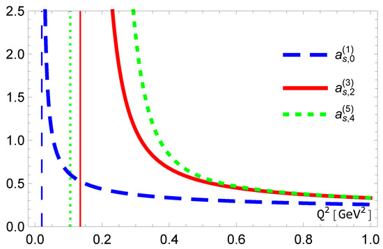
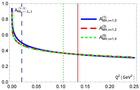
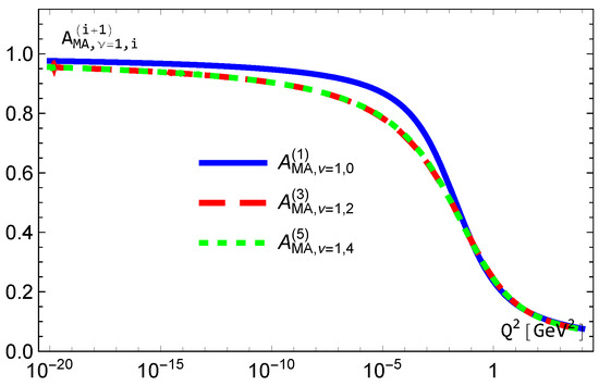
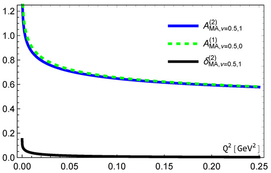
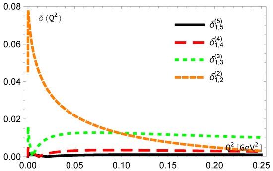
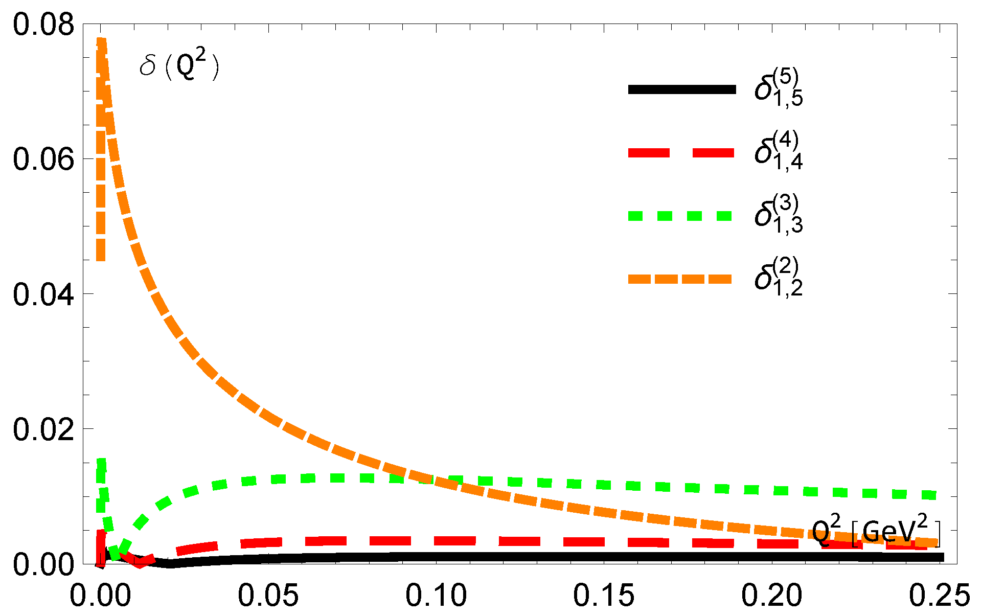
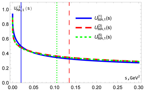
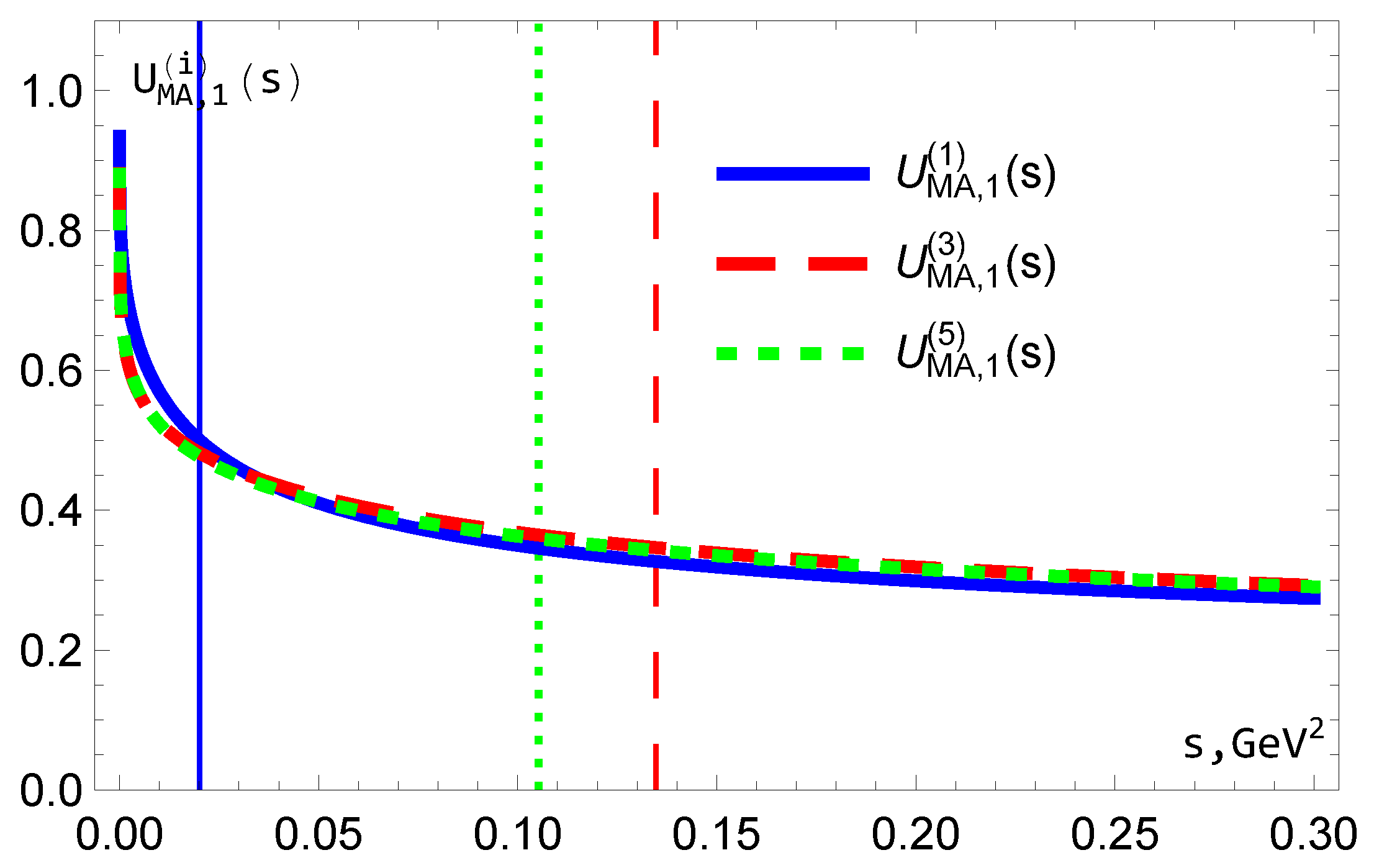
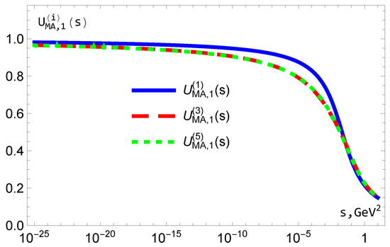
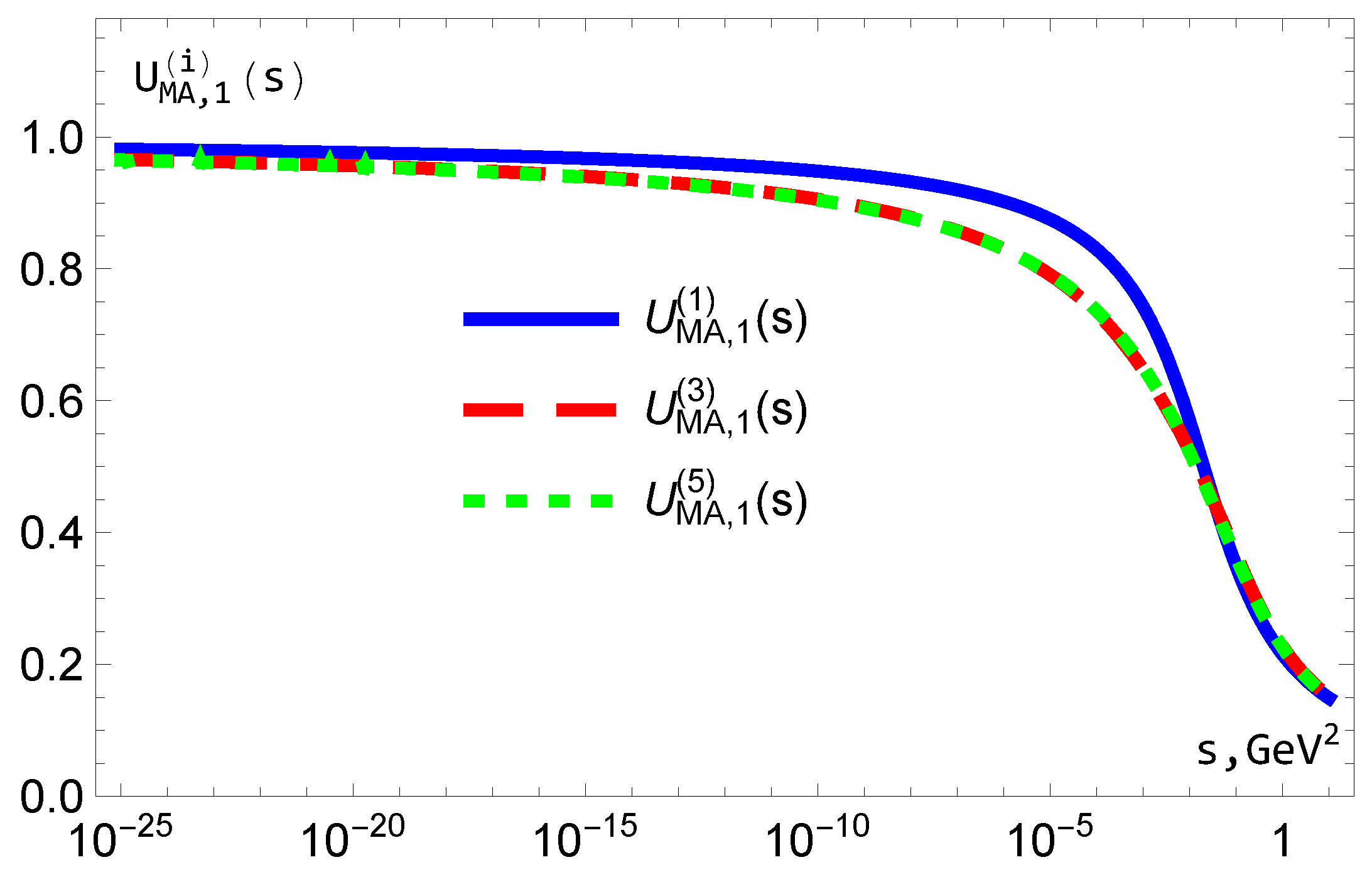
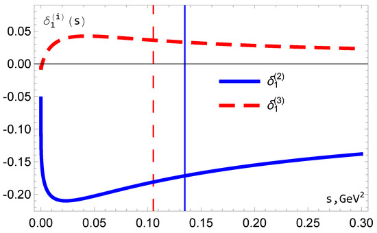
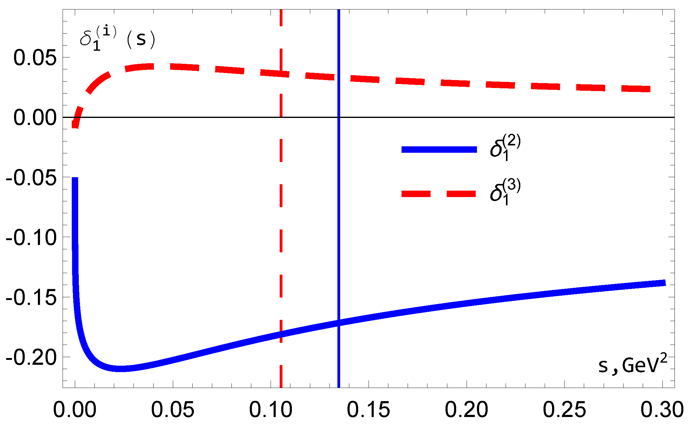
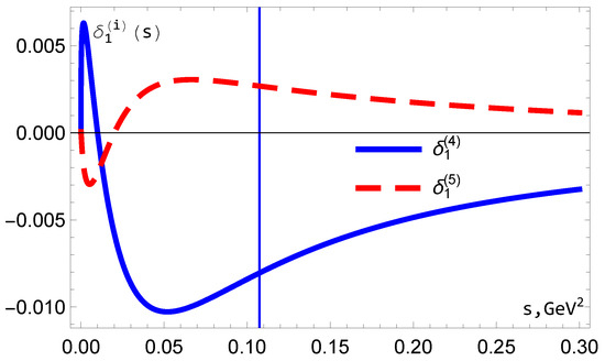
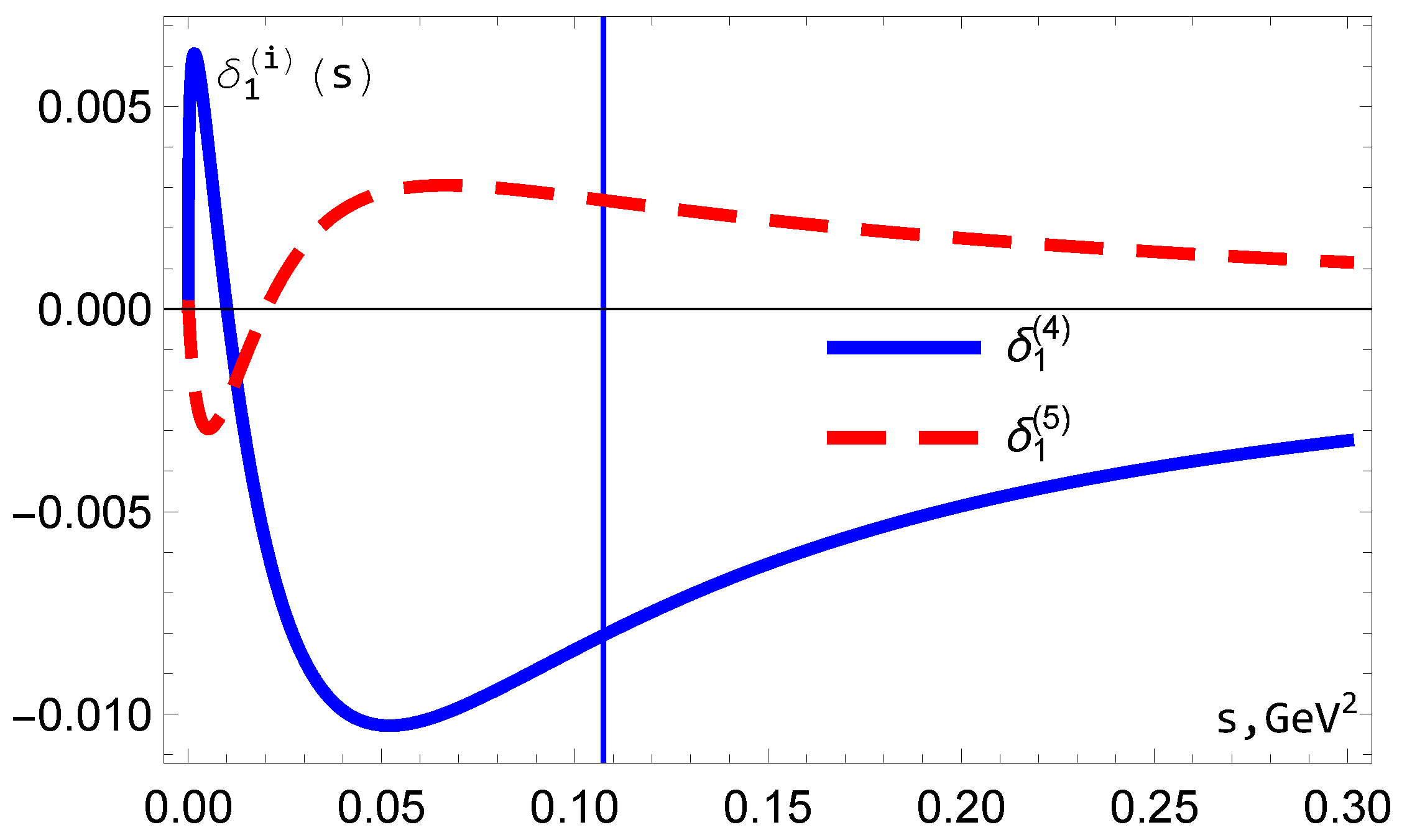
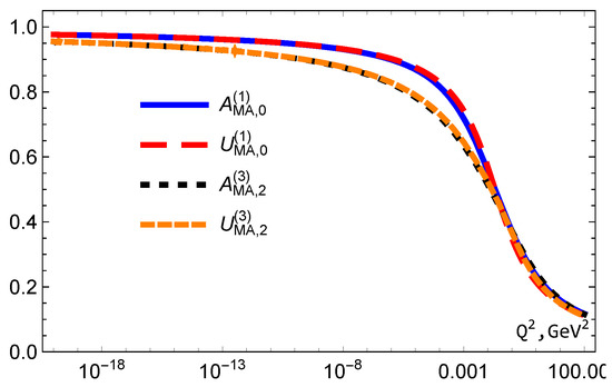
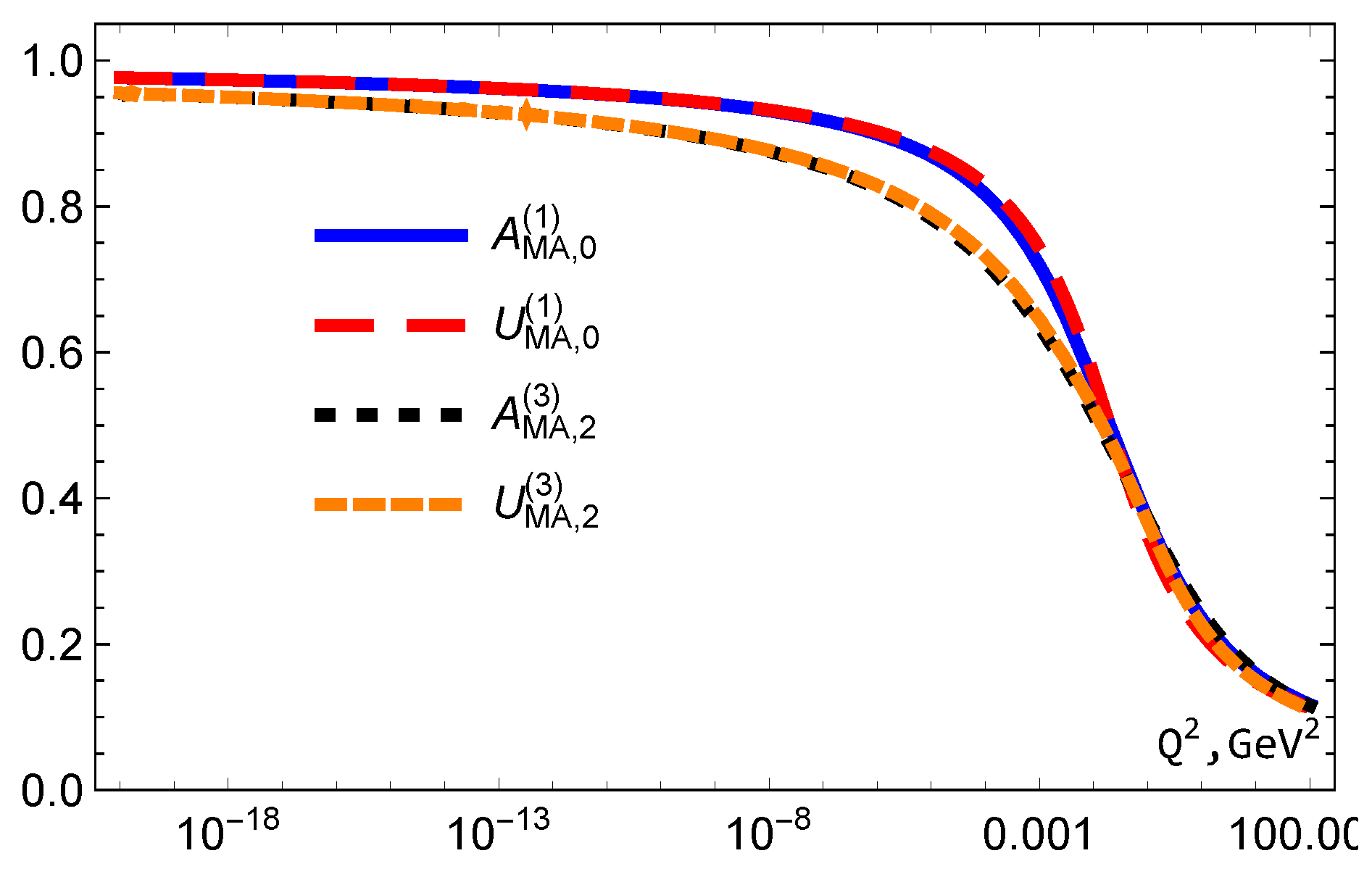
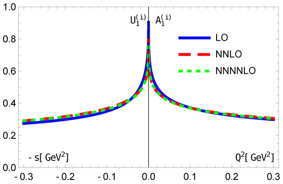
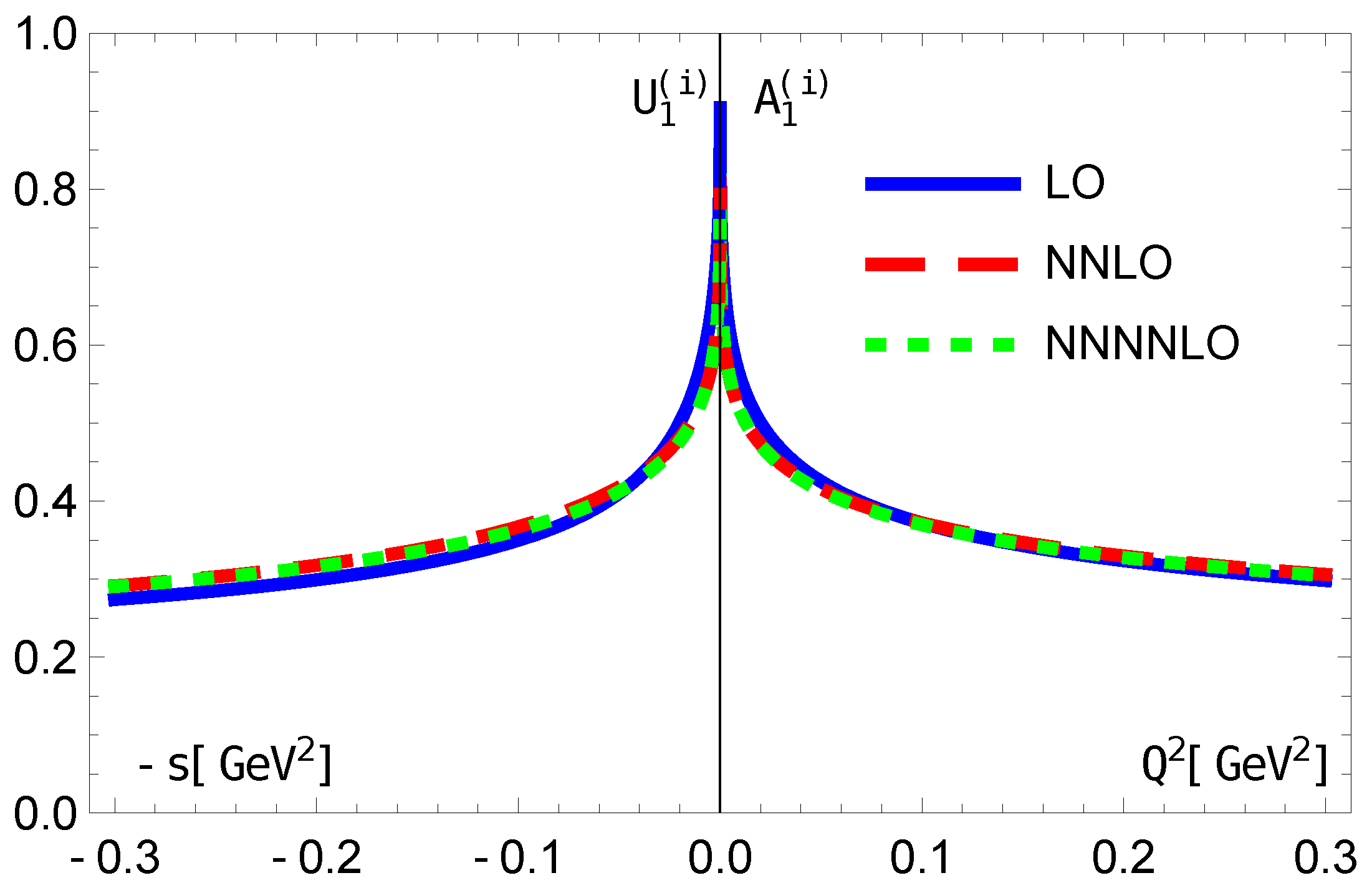
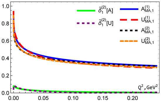
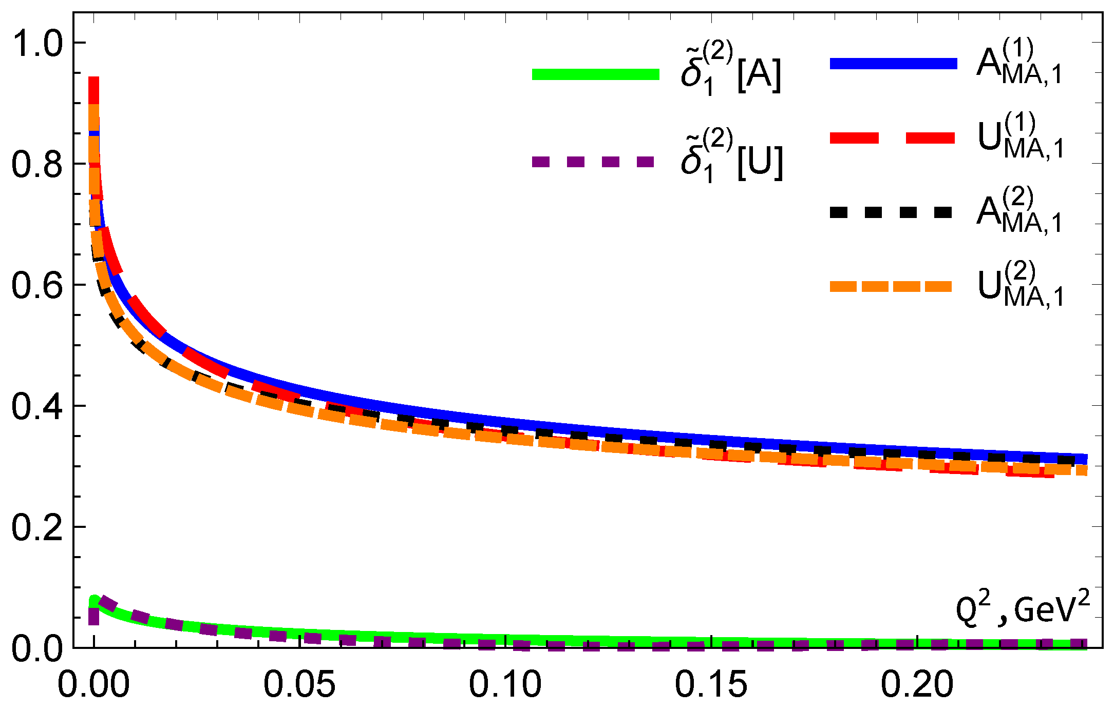
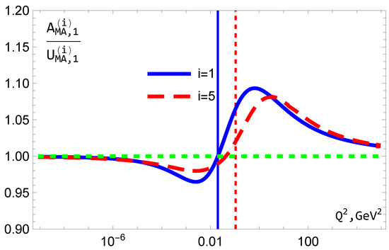
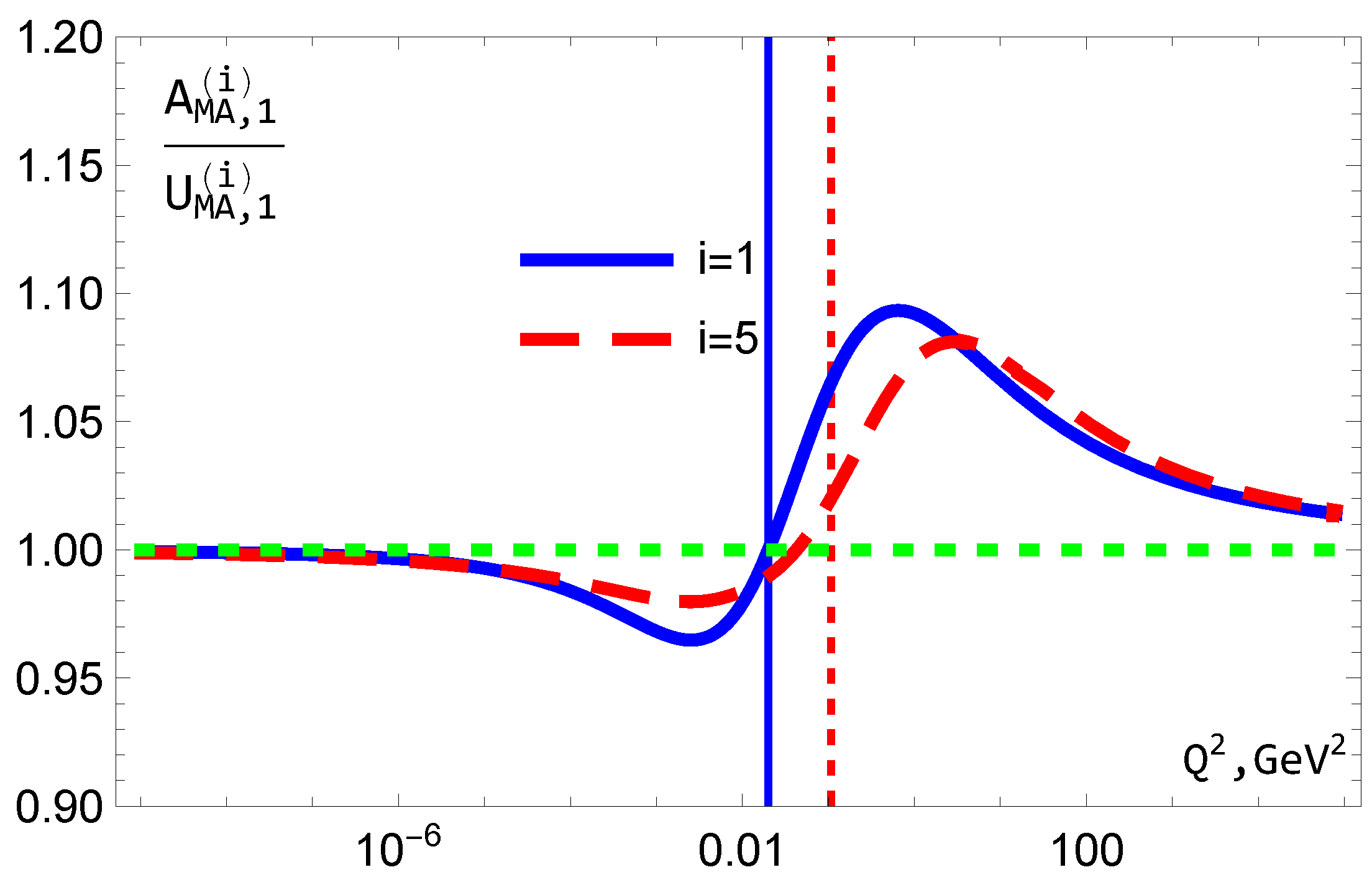
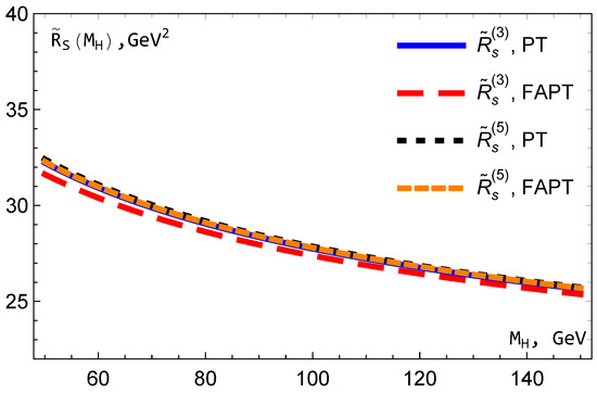
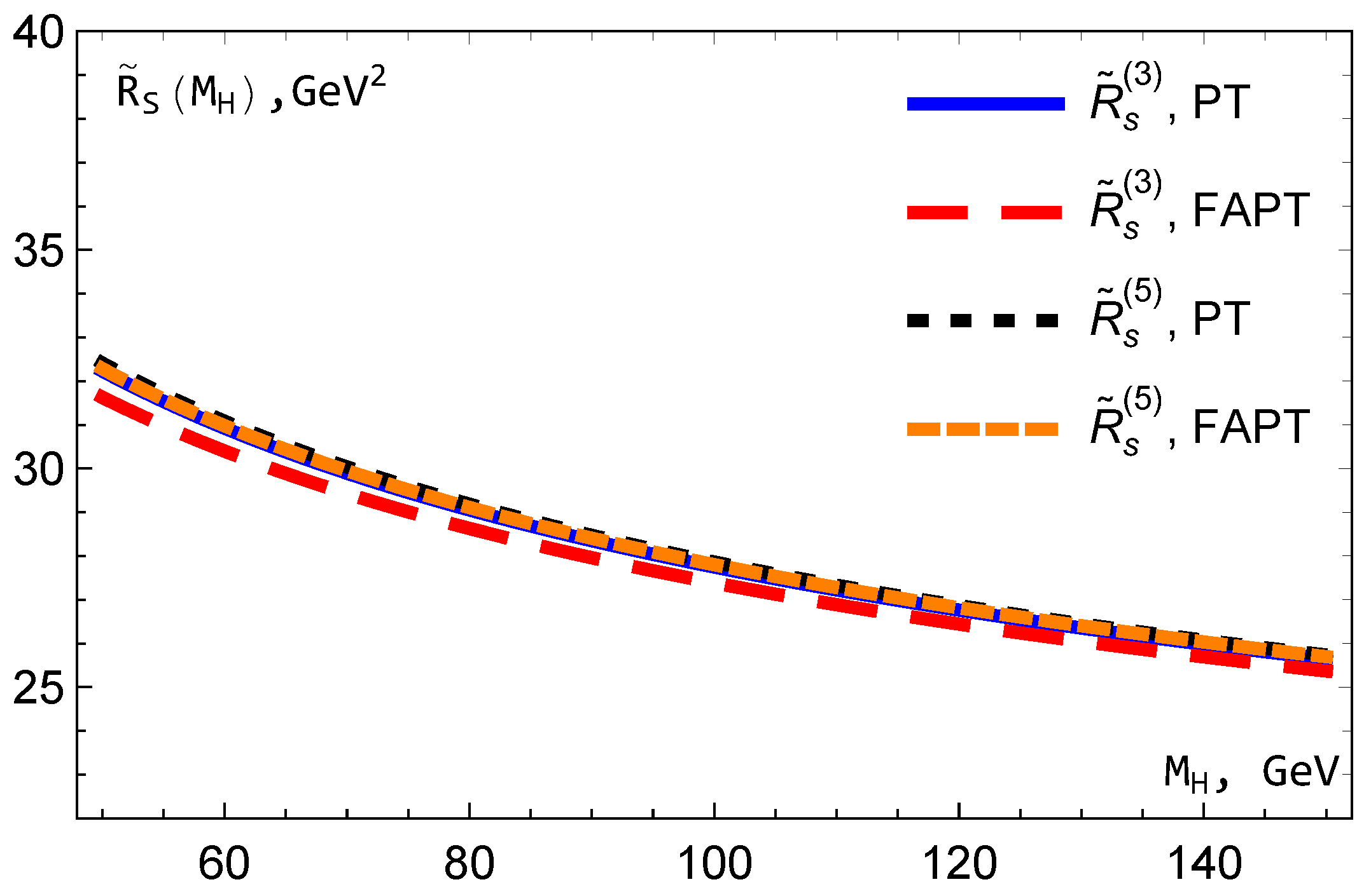
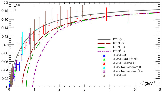
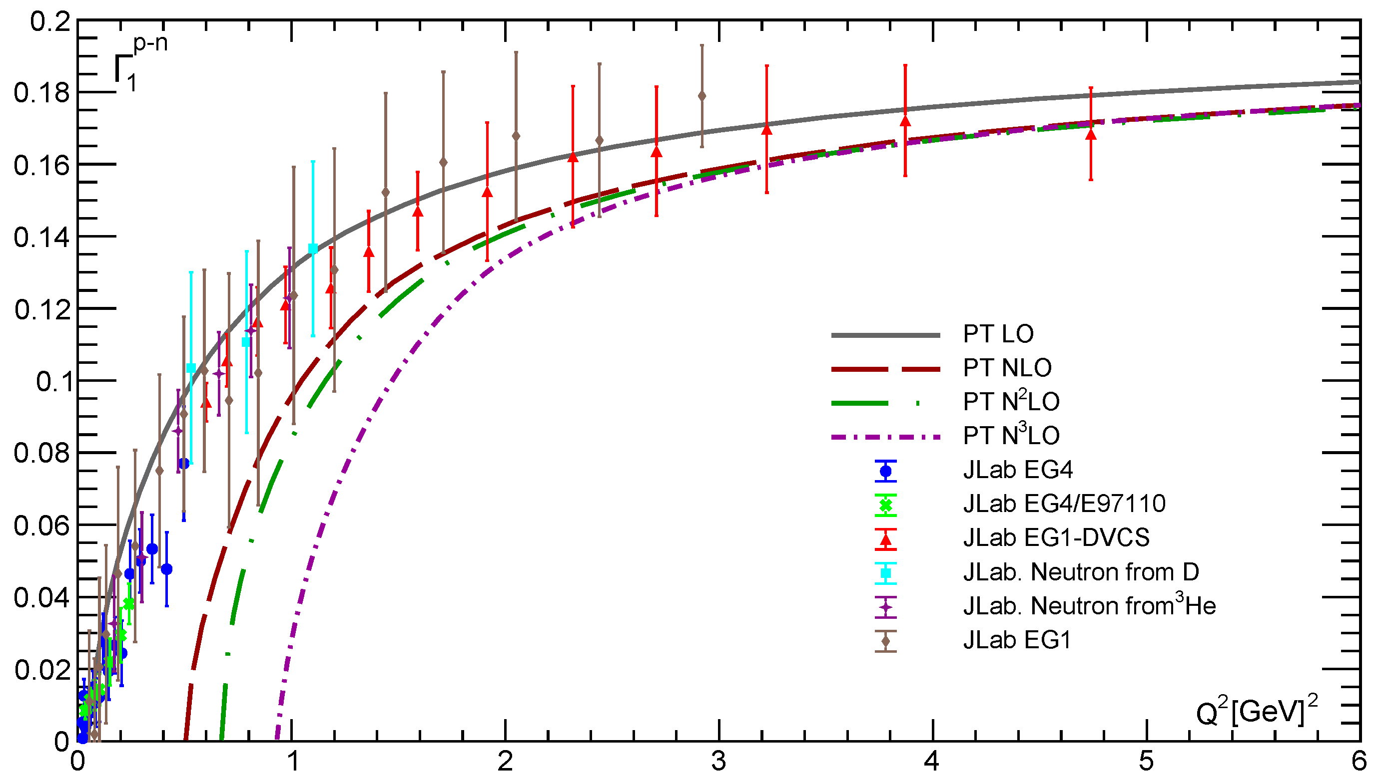
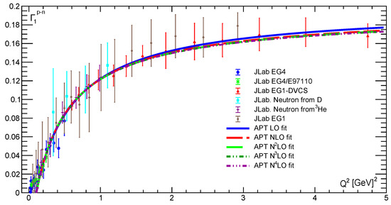
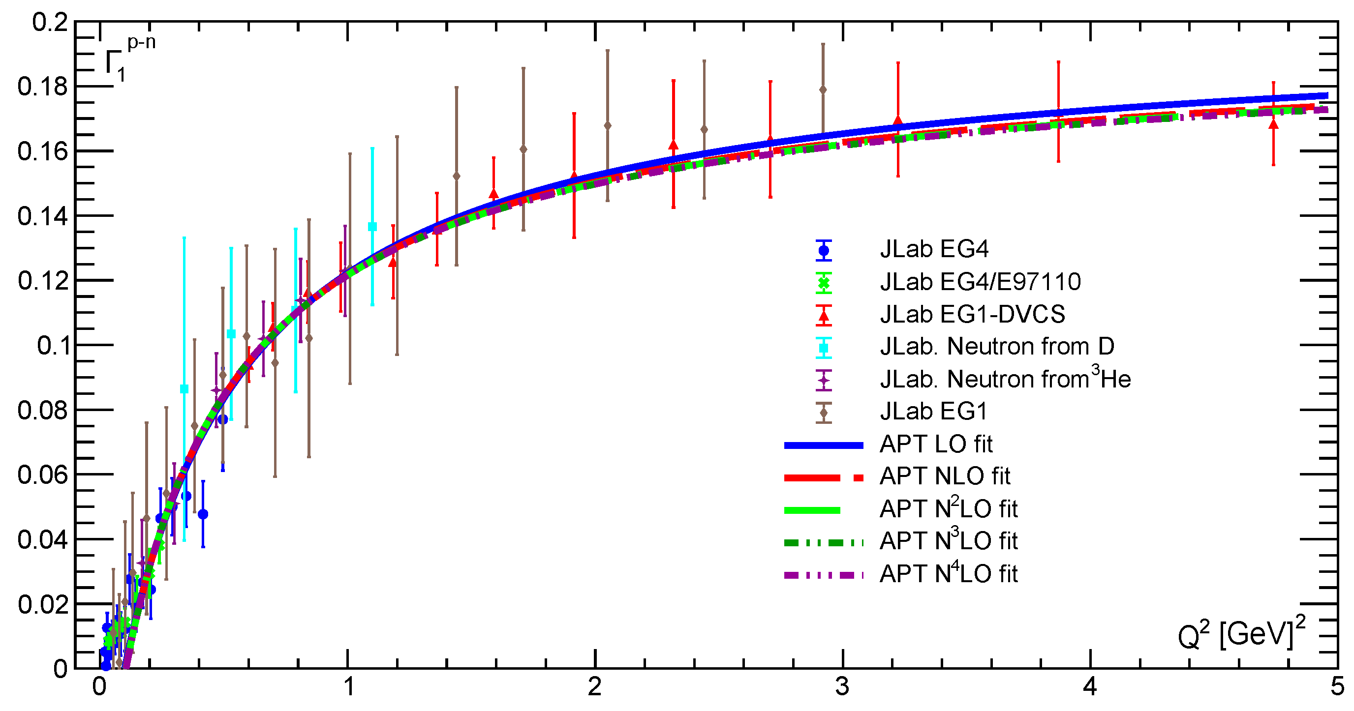
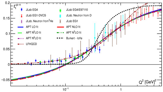
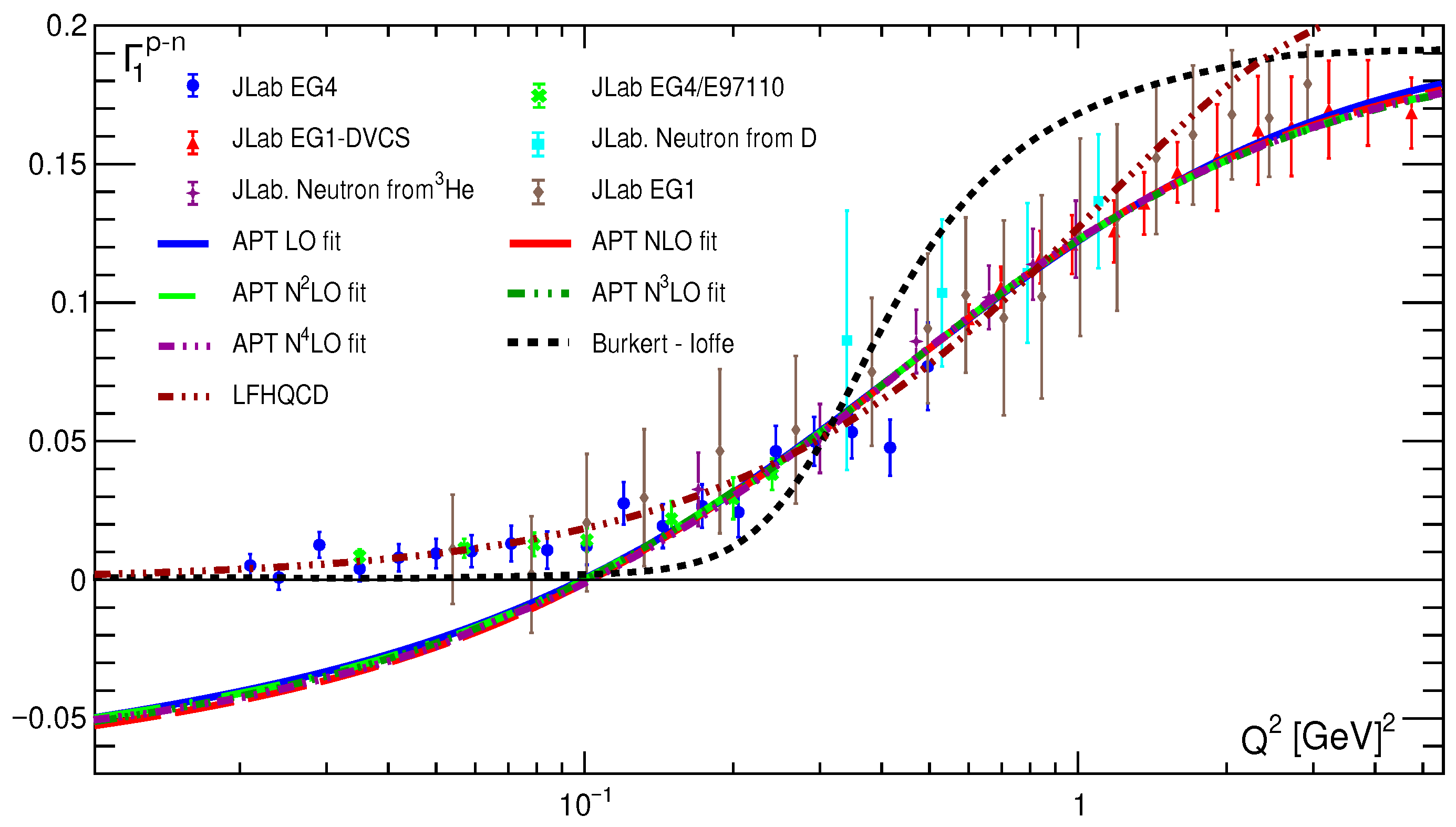
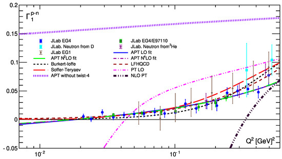
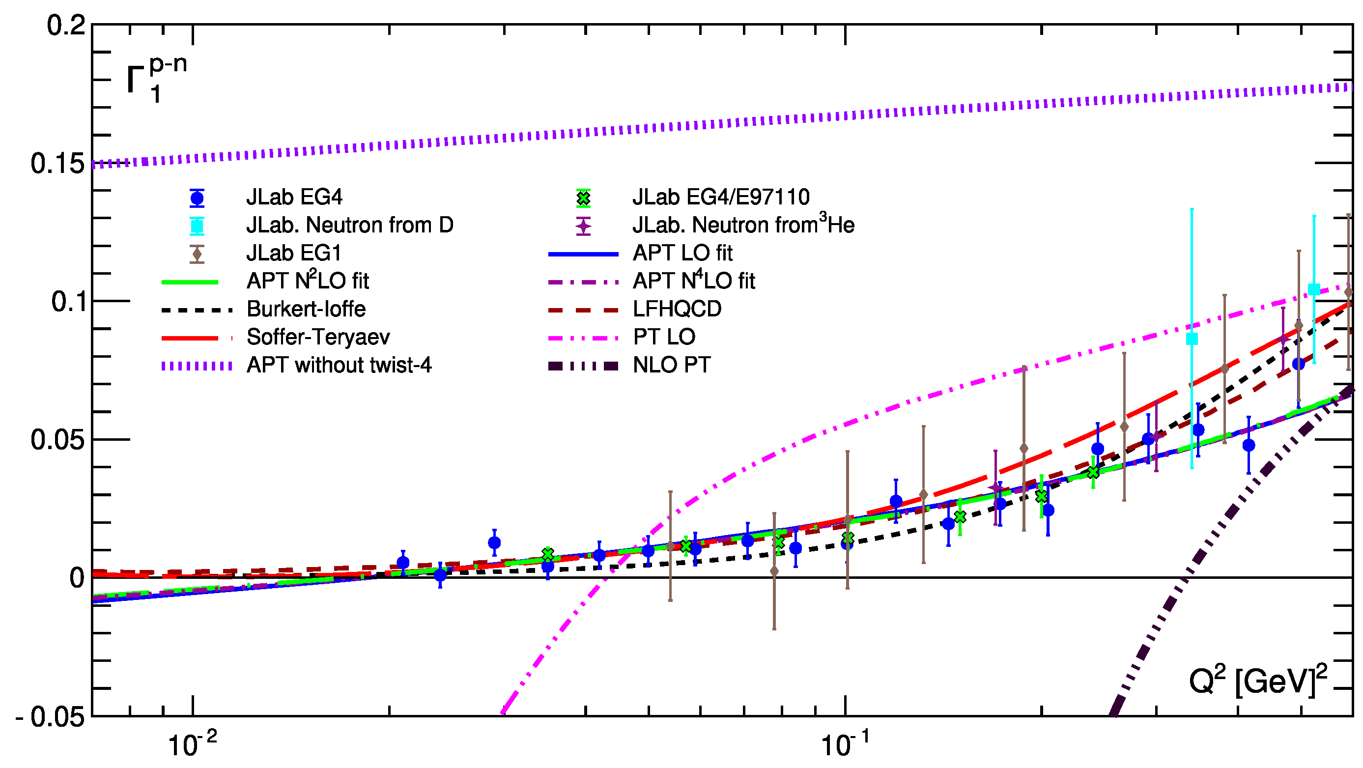
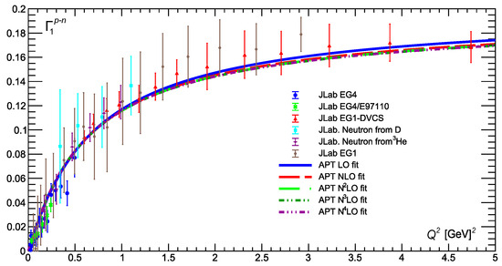
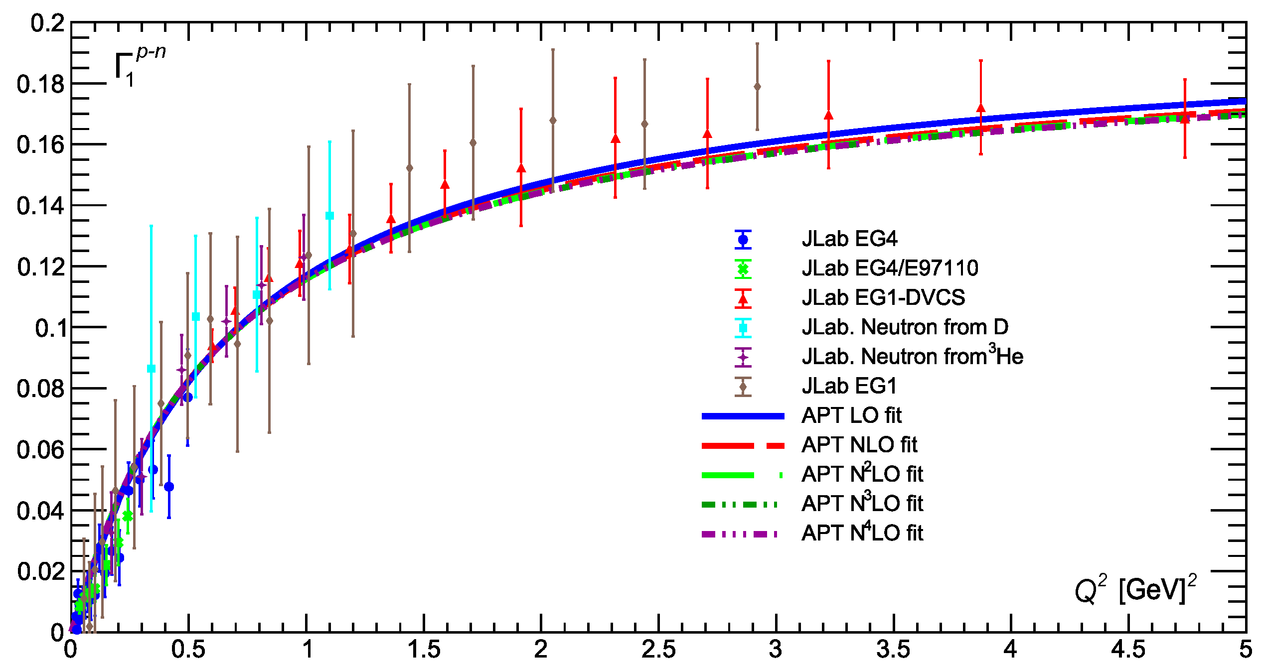
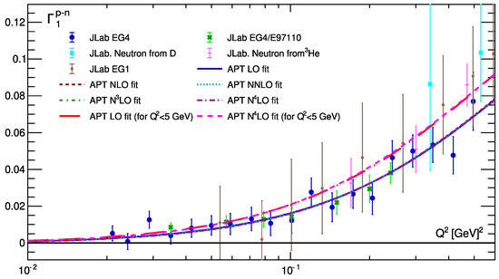
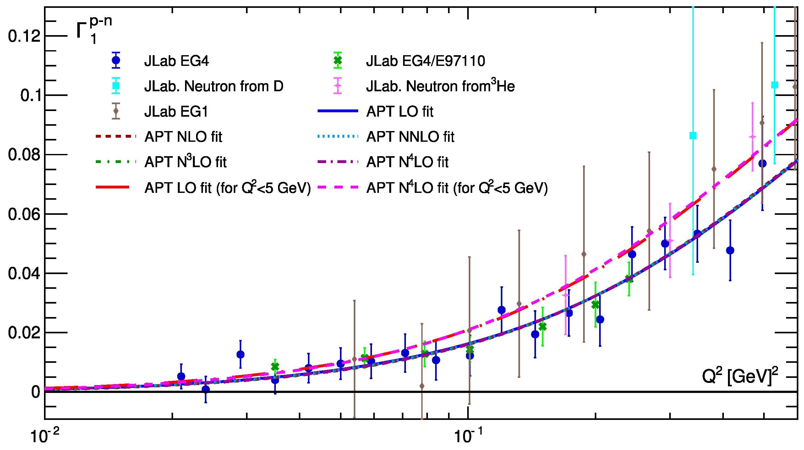

Disclaimer/Publisher’s Note: The statements, opinions and data contained in all publications are solely those of the individual author(s) and contributor(s) and not of MDPI and/or the editor(s). MDPI and/or the editor(s) disclaim responsibility for any injury to people or property resulting from any ideas, methods, instructions or products referred to in the content. |
© 2025 by the authors. Licensee MDPI, Basel, Switzerland. This article is an open access article distributed under the terms and conditions of the Creative Commons Attribution (CC BY) license (https://creativecommons.org/licenses/by/4.0/).