In-Plane Vibration Analysis of Annular Plates Considering All Combinations of Edge Conditions

Abstract

The Ritz method is applied to an in-plane vibration analysis to obtain accurate frequencies of isotropic annular plates. The method is formulated in a manner that allows all combinations of free boundary conditions, two types of supported (constraining only either radial or circumferential displacement) boundary conditions, and clamped boundary conditions. Admissible functions for the two displacement components are chosen as products of trigonometric functions in the circumferential coordinate and special algebraic polynomials in the radial coordinate, enabling all possible boundary-condition combinations to be satisfied. In the numerical study, after the solution’s accuracy is verified through convergence and comparison tests, extensive and accurate frequency parameters are presented to cover all combinations of the four in-plane boundary conditions along the outer and inner edges of the annular plates.

1. Introduction

Out-of-plane (bending) vibration of annular circular plates has been studied extensively. In addition to the early landmark papers [1,2], very recent works on the topic have also been published [3,4], and other relevant studies over the past few decades are summarized in [4]. In contrast, studies on in-plane vibration are limited because it is difficult to derive solutions from the governing equations, which involve two independent displacement components.

For in-plane vibration, the first publication presenting a reasonable amount of numerical results was reported in 1984 by Irie et al. [5] using the transfer matrix method. They provided lists of natural frequencies of thin annular plates with free or clamped edges at their outer and inner boundaries (four combinations, i.e., two by two), but did not include the supported condition (i.e., an edge constraint intermediate between free and clamped). Bashmal et al. [6] derived approximate solutions by using ritz method and presented numerical results for only the same four cases as in [5]. Ravari and Forouzan [7] presented an analytical approach incorporating polar orthotropy in the plate. Shi and his colleagues [8,9] investigated the in-plane vibration of annular plates with translational springs acting on both displacement components. Wang et al. [10] introduced what they termed the modified Fourier series expansion and artificial boundary spring technique, and constructed a model of an annular plate using a set of annular sector elements elastically restrained at the edges. In 2019, Lyu et al. [11] considered the problem of a rotating annular plate with elastic boundaries and presented the effect of rotational speed on the natural frequencies. Recently, Guan and his colleagues [12] solved the in-plane vibration problem of polar-orthotropic annular plates and conducted a parametric study to clarify the effects of orthotropy. A related new study on in-plane vibration was published in 2025 in connection with the in-plane vibration of spinning annular plate systems [13].

As reviewed above, only a limited number of studies have addressed the in-plane vibration of annular plates. Moreover, comprehensive numerical investigations covering all sixteen boundary-condition cases have not yet been conducted. Specifically, each of the outer and inner edges may be constrained by one of four boundary conditions: free (F), two types of supported edges (S1 and S2), and clamped (C). Therefore, the objective of the present study is to summarize the possible sets of natural frequencies for all sixteen combinations of boundary conditions in annular plates and to provide a complete set of reference data for accurate natural frequencies of this problem.

In this study, an energy function composed of elastic and kinetic energies is formulated, and the Ritz method is applied. Unlike conventional applications of the Ritz method, the present approach employs special displacement functions incorporating boundary indices, making the formulation applicable to any combination of edge conditions along the outer and inner boundaries. A finite element formulation is also developed by the author (without using commercial FEM software) to obtain natural frequencies for comparison with the present Ritz results. The numerical study includes comparisons between the present Ritz results, those obtained from the self-developed FEM code, and previously published results, in order to establish the validity of the proposed approaches.

Following this validation, sixteen tables are provided to summarize the frequency parameters for all combinations of the four boundary conditions (F, S1, S2, and C) at the outer and inner edges, and for five different hole ratios (defined as the ratio of inner radius to outer radius). It is hoped that these comprehensive and complete sets of frequency parameters will be useful for mechanical designs involving the in-plane vibration of annular plate models, such as rotating conventional and piezoelectric disks, railway brake disks, and related structures.

2. Vibration Analysis

2.1. Ritz Method

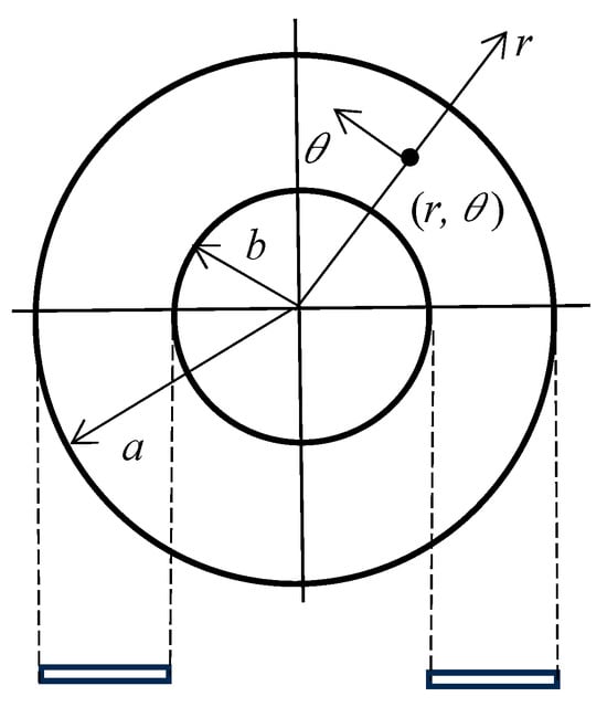
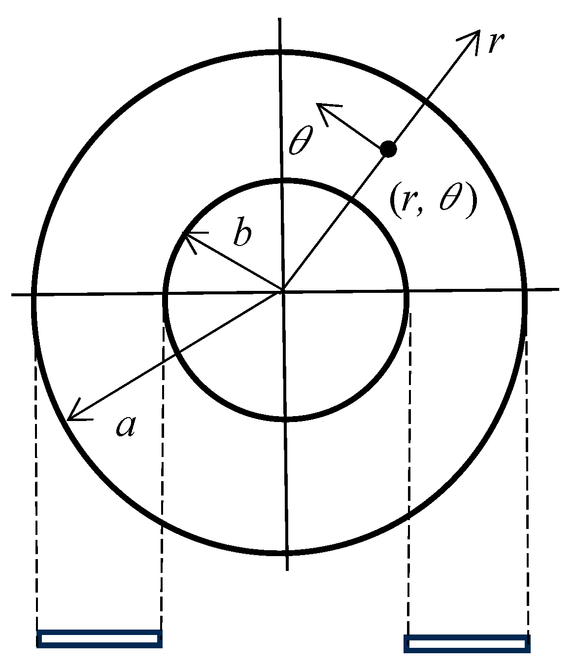
Free in-plane vibration of an annular plate is analyzed in polar coordinates, as shown in Figure 1. Outer and inner radii are given by a and b, respectively, and the uniform thickness is given by h. The plate is subjected to any combination of in-plane boundary conditions along its outer and inner edges, but this does not include elastic edge conditions (i.e., edges constrained by springs).

Figure 1. Annular plate in the polar coordinates.

Assuming sinusoidal time variation in radian frequency ω, the maximum in-plane strain energy of the plate is expressed in the form of

$$U={\displaystyle \frac{1}{2}}{\displaystyle {\int }_b^a{\displaystyle {\int }_0^{2\pi }{\left\{\epsilon \right\}}^T\left[A\right]}}\left\{\epsilon \right\}rd\theta dr$$

(1)

with

$$\left\{\epsilon \right\}=\left\{\begin{array}{c}{\displaystyle \frac{\partial u}{\partial r}}\\ {\displaystyle \frac{1}{r}}\left(u+{\displaystyle \frac{\partial v}{\partial \theta }}\right)\\ {\displaystyle \frac{1}{r}}\left({\displaystyle \frac{\partial u}{\partial \theta }}-v\right)+{\displaystyle \frac{\partial v}{\partial r}}\end{array}\right\},\begin{array}{c}\end{array}\left[A\right]=\left[\begin{array}{ccc}{A}_{11}& A_{12}& 0\\ A_{12}& A_{22}& 0\\ 0& 0& A_{66}\end{array}\right]$$

(2)

where u(r,θ) and v(r,θ) are the in-plane amplitudes of the plate in the radial and circumferential directions, respectively. For a polar–orthotropic material, the set of in-plane stiffness is defined by

$$A_{11}=A_r={\displaystyle \frac{E_{r}h}{1-{\nu }_r{\nu }_{\theta }}},A_{22}=A_{\theta }={\displaystyle \frac{E_{\theta }h}{1-{\nu }_r{\nu }_{\theta }}},A_{12}={\nu }_r{A}_{\theta }={\nu }_{\theta }{A}_r,A_{66}=G_{r\theta }h$$

(3)

where E_r and E_θ are Young’s moduli in the r and θ directions, respectively, G_rθ is the shear modulus, and ν_r and ν_θ are the major and minor Poisson’s ratios. For an isotropic material, Equation (3) is reduced to

$$A_{11}=A_{22}={\displaystyle \frac{Eh}{1-{\nu }^2}},\begin{array}{c}{A}_{12}=\nu A_{11},A_{66}\end{array}={\displaystyle \frac{Eh}{2\left(1+\nu \right)}}$$

(4)

The maximum in-plane kinetic energy of the plate is

$$T={\displaystyle \frac{1}{2}}\rho h{\omega }^2{\displaystyle {\int }_b^a{\displaystyle {\int }_0^{2\pi }\left(u^2+v^2\right)rd\theta dr}}$$

(5)

where ρ is the average mass of the plate per unit volume.

The separation of variables is assumed to be

$$u\left(r,\theta \right)=U\left(r\right)\cos n\theta ,\begin{array}{c}\end{array}v\left(r,\theta \right)=V\left(r\right)\sin n\theta$$

(6)

where U(r) and V(r) are functions in the radial direction, n is an integer to prescribe the number of nodal diameters. Equation (6) is substituted into Equations (1) and (5) by integrating in the circumferential direction, and one gets

$$U={\displaystyle \frac{\pi }{2}}{\displaystyle {\int }_b^a{\left\{\epsilon \right\}}^T\left[A\right]\left\{\epsilon \right\}rdr},\begin{array}{c}\end{array}T={\displaystyle \frac{\pi }{2}}\rho h{\omega }^2{\displaystyle {\int }_b^a\left(U^2+V^2\right)rdr}$$

(7)

where {ε} becomes

$$\left\{\epsilon \right\}=\left\{\begin{array}{c}{\displaystyle \frac{dU}{dr}}\\ {\displaystyle \frac{1}{r}}\left(U+nV\right)\\ -{\displaystyle \frac{1}{r}}\left(nU+V\right)+{\displaystyle \frac{dV}{dr}}\end{array}\right\}$$

(8)

The resulting function is given for the problem by

$$F=T-U$$

(9)

For simplicity of analysis, the following variables are introduced in non-dimensional form as

$$\begin{array}{l}\eta =r/a\begin{array}{c}\end{array}\left(\mathrm{non}-\mathrm{dimensional}\begin{array}{c}\end{array}\mathrm{radial}\begin{array}{c}\end{array}\mathrm{coodinate}\right),\begin{array}{c}\end{array}\\ \alpha =b/a\begin{array}{c}\end{array}\left(\mathrm{aspect} \mathrm{ratio} \mathrm{of} \mathrm{inner} \mathrm{and} \mathrm{outer} \mathrm{radius}\right),\\ \begin{array}{c}\Omega =\omega a\sqrt{{\displaystyle \frac{\rho \left(1-{\nu }^2\right)}{E}}}\end{array}\left(\mathrm{non}-\mathrm{dimensional} \mathrm{frequency} \mathrm{for} \mathrm{isotropic} \mathrm{plate}\right),\begin{array}{c}\end{array}\\ aij=Aij/A11\begin{array}{c}\end{array}\left(i,j=1,2,6\right)\end{array}$$

(10)

As is widely known, it is important in the Ritz method to introduce effective trial functions to simulate the accurate vibrating displacement (amplitude). The functions U(η) and V(η) in Equation (6) are assumed here as

$$\begin{gathered} U\left(\eta ,i\right)={\displaystyle \sum _{i=0}^{M-1}{U}_i{\eta }^i}{\left(\eta -1\right)}^{Bu1}{\left(\eta -\alpha \right)}^{Bu2}, V\left(\eta ,j\right)={\displaystyle \sum _{j=0}^{M-1}{V}_j{\eta }^j}{\left(\eta -1\right)}^{Bv1}{\left(\eta -\alpha \right)}^{Bv2} \\ \hspace{1em}\hspace{1em}\hspace{1em}\hspace{1em} \left(U_i,V_j: \mathrm{unknown} \mathrm{coefficients}\right) \end{gathered}$$

(11)

where these polynomial functions have the boundary index Bu1, …, Bv2 (1: outer, 2: inner edge) to prescribe the kinematical boundary conditions.

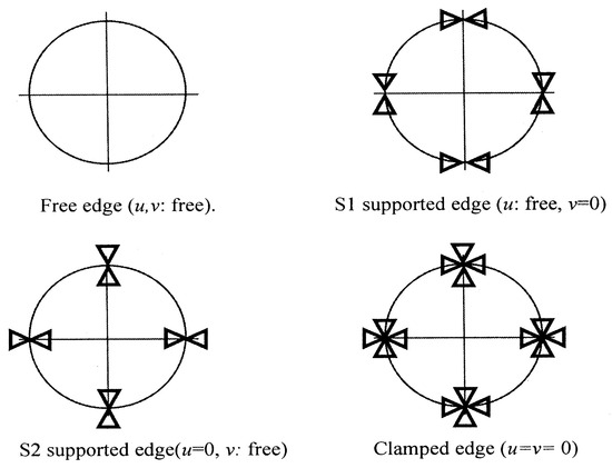
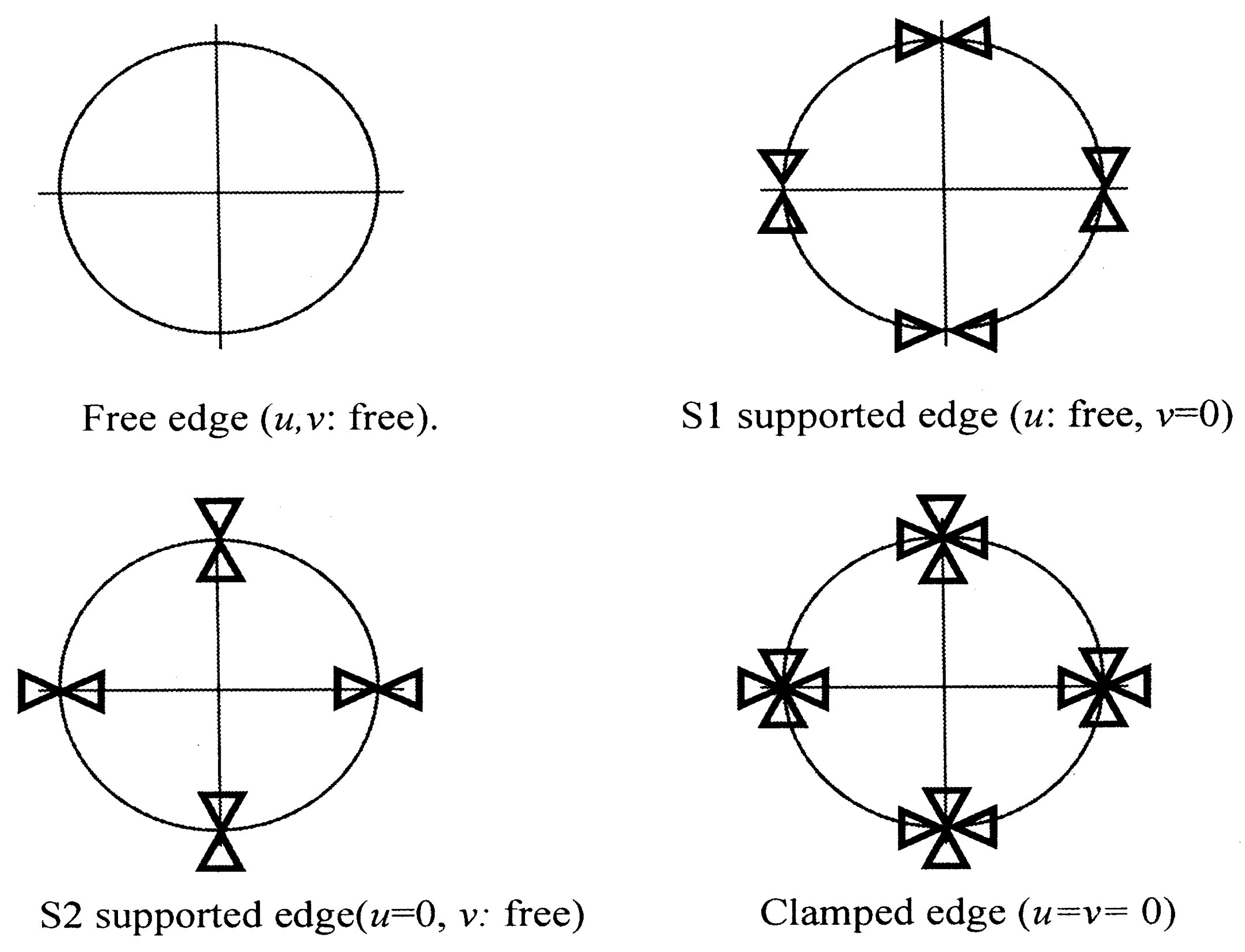
The index is taken as “Bu1 = 0 or 1” and “Bv1 = 0 or 1” at the outer edge, and “Bu2 = 0 or 1” and “Bv2 = 0 or 1” at the inner edge, where index “0” indicates free and “1” indicates constrained. Therefore, “four combinations times four (4 × 4 = 16)” different combinations are possible for the in-plane vibration of an annular plate. As shown in Figure 2, these four choices at one edge are labeled as F (Free, u and v are both free (zero normal stress both in radial and circumferential directions)), S1 (Support type 1: u is free (zero normal stress in radial direction)) but v = 0), S2 (Support type 2: u = 0 but v is free (zero normal stress in circumferential direction) and C (u and v are both zero).

Figure 2. Illustration of four types of uniform constraints along the inner or outer edge.

A frequency equation is derived by applying the Ritz process to extremize the function (9) as

$${\displaystyle \frac{\partial F}{\partial U_{\overline{i}}}}={\displaystyle \frac{\partial F}{\partial V_{\overline{j}}}}=0\begin{array}{c}\end{array}\left(\overline{i},\overline{j}=0,1,2,\dots ,M-1\right)$$

(12)

For a specific n, eigenvalues (non-dimensional frequency parameter) Ω are extracted from the frequency equation

$$\left[\begin{array}{cc}{\displaystyle \sum _{i=0}^{M-1}{F}_{11}}& {\displaystyle \sum _{j=0}^{M-1}{F}_{12}}\\ sym& {\displaystyle \sum _{j=0}^{M-1}{F}_{22}}\end{array}\right]\left\{\begin{array}{c}{U}_i\\ V_j\end{array}\right\}=0\begin{array}{c}\end{array}\left(\overline{i},\overline{j}=0,1,2,\dots ,M-1\right)$$

(13)

where

$$\begin{array}{l}{F}_{11}=a_{11}{I}_{1,i\overline{i}}^{\left(11\right)}+a_{12}\left(I_{0,i\overline{i}}^{\left(10\right)}+I_{0,i\overline{i}}^{\left(01\right)}\right)+a_{22}{I}_{-1,i\overline{i}}^{\left(00\right)}+a_{66}{n}^2{I}_{-1,i\overline{i}}^{\left(00\right)}-{\Omega }^2{I}_{1,i\overline{i}}^{\left(00\right)}\\ F_{12}=n\left\{a_{12}{I}_{0,j\overline{i}}^{\left(01\right)}+a_{22}{I}_{-1,j\overline{i}}^{\left(00\right)}+a_{66}\left(I_{-1,j\overline{i}}^{\left(00\right)}-I_{0,j\overline{i}}^{\left(10\right)}\right)\right\}\\ F_{22}=a_{22}{n}^2{I}_{-1,j\overline{j}}^{\left(00\right)}+a_{66}\left(I_{-1,j\overline{j}}^{\left(00\right)}+I_{1,j\overline{j}}^{\left(11\right)}-I_{0,j\overline{j}}^{\left(10\right)}-I_{0,j\overline{j}}^{\left(01\right)}\right)-{\Omega }^2{I}_{1,j\overline{j}}^{\left(00\right)}\end{array}$$

(14)

with

$$\begin{array}{l}{I}_{k,i\overline{i}}^{\left(\mathrm{pq}\right)}={\displaystyle {\int }_{\alpha }^1{\eta }^k\frac{d^{\left(\mathrm{p}\right)}U\left(\eta ,i\right)}{d{\eta }^{\left(\mathrm{p}\right)}}}{\displaystyle \frac{d^{\left(\mathrm{q}\right)}U\left(\eta ,\overline{i}\right)}{d{\eta }^{\left(\mathrm{q}\right)}}}d\eta ,\begin{array}{c}\end{array}\\ I_{k,j\overline{i}}^{\left(\mathrm{pq}\right)}={\displaystyle {\int }_{\alpha }^1{\eta }^k\frac{d^{\left(\mathrm{p}\right)}V\left(\eta ,j\right)}{d{\eta }^{\left(\mathrm{p}\right)}}}{\displaystyle \frac{d^{\left(\mathrm{q}\right)}U\left(\eta ,\overline{i}\right)}{d{\eta }^{\left(\mathrm{q}\right)}}}d\eta ,\\ I_{k,j\overline{j}}^{\left(\mathrm{pq}\right)}={\displaystyle {\int }_{\alpha }^1{\eta }^k\frac{d^{\left(\mathrm{p}\right)}V\left(\eta ,j\right)}{d{\eta }^{\left(\mathrm{p}\right)}}}{\displaystyle \frac{d^{\left(\mathrm{q}\right)}V\left(\eta ,\overline{j}\right)}{d{\eta }^{\left(\mathrm{q}\right)}}}d\eta \end{array}$$

(15)

Integration is carried out in the exact manner (not by using numerical integration) and the eigenvalues are extracted with the help of the eigenvalue subroutine.

2.2. Finite Element Formulation

The present finite element formulation is based on the same linear elastic theory as in Section 2.1. A pair of in-plane amplitudes are assumed in the r and θ directions, after having assumed sinusoidal time variation, as

$$\left\{\begin{array}{c}U\left(r\right)\\ V\left(r\right)\end{array}\right\}=\left[P\right]\left\{\beta \right\}$$

(16)

where

$$\left[P\right]=\left[\begin{array}{cccc}1& 0& r& 0\\ 0& 1& 0& r\end{array}\right],\left\{\beta \right\}={\left\{{\beta }_0,{\gamma }_0,{\beta }_1,{\gamma }_1\right\}}^T$$

(17)

By using a one-dimensional element with specified coordinates r = ri and r = rj at two ends, the element displacement vector at the two ends (nodes) is expressed by

$$\left\{d_e\right\}={\left\{u_i,v_i,u_j,v_j\right\}}^T$$

(18)

Substitution of Equation (16) into the coordinates at the two ends of the one-dimensional element yields

$$\left\{d_e\right\}=\left[C\right]\left\{\beta \right\},\begin{array}{c}\end{array}\mathrm{i}.\mathrm{e}.,\begin{array}{c}\end{array}\left\{\beta \right\}={\left[C\right]}^{-1}\left\{d_e\right\}$$

(19)

A strain vector in Equation (8) is written in the form

$$\left\{\epsilon \right\}=\left[Q\right]\left\{\beta \right\}=\left[Q\right]{\left[C\right]}^{-1}\left\{d_e\right\}$$

(20)

An element strain vector is obtained by substituting Equation (20) into (7) as

$$U_e={\displaystyle \frac{1}{2}}{\left\{d_e\right\}}^T\left[K_e\right]\left\{d_e\right\}$$

(21)

for one element, where [K_e] is the element stiffness matrix

$$\left[K_e\right]={\left({\left[C\right]}^{-1}\right)}^T·{\displaystyle {\int }_{ri}^{rj}{\left[Q\right]}^T\left[A\right]\left[Q\right]d}r\begin{array}{c}\end{array}·{\left[C\right]}^{-1}$$

(22)

In a similar fashion, an element mass matrix is derived in the form

$$T_e={\displaystyle \frac{1}{2}}\rho h{\omega }^2{\left\{d_e\right\}}^T\left[M_e\right]\left\{d_e\right\}$$

(23)

where ω is a radian frequency, and [M_e] is an element mass matrix

$$\left[M_e\right]={\left({\left[C\right]}^{-1}\right)}^T·{\displaystyle \int \left(U^2+V^2\right)dr}·{\left[C\right]}^{-1}$$

(24)

The element stiffness and mass matrices are located in the global system, and then the global system is assembled as

$$\left(\left[K\right]-\rho h{\omega }^2\left[M\right]\right)\left\{\delta \right\}=0$$

(25)

where [K], [M] and {δ} are the global stiffness matrix, global mass matrix and global displacement vector, respectively. As in the Ritz method, eigenvalues ω² are extracted from the equation, and the radian frequency is modified as a dimensionless frequency parameter to Ω in Equation (10).

3. Numerical Results and Discussions

Numerical results are given for isotropic annular plates with all possible sets of boundary conditions at the outer and inner edges. Figure 2 presents four different boundary conditions along either one of the two edges. Along the “Free edge (abbreviated as F)”, two in-plane displacements in the radial and circumferential directions are not constrained at all, and the corresponding two normal stresses are zero. “S1-supported edge (S1)” indicates that the displacement in the circumferential direction is uniformly zero (due to space limit, only four discrete symbols are given in the figure), but the displacement in the radial direction is free. Vice versa, “S2 support edge (S2)” indicates that the displacement in the radial direction is zero and the circumferential displacement is unconstrained along the edge. Finally, “clamped edge (C)” means that both displacements are uniformly zero.

For an annular plate, the number of combinations ends up as the sixteen combinations given by “four boundary conditions times four”. The natural frequencies for all combinations are presented in the form of frequency parameter Ω, and the lowest eight parameters are summarized for five aspect ratios b/a = 0.1, 0.2, 0.3, 0.4 and 0.5. Comparisons between the Ritz and FEM results are given in all tables with four significant figures. This thoroughness of presentation is one of the purposes of this study.

Table 1 summarizes the convergence of the present Ritz method and the self-developed FEM (hereafter, the note “present” or “self-developed” is omitted), and the terms “Ritz” and “FEM” simply denote the results obtained by the author. The lowest eight frequency parameters are presented in four significant figures together with the mode indices (n,s). Identical values (to four significant figures) are underlined when they are found to coincide during the convergence process. This table considers two sets of boundary conditions, namely S1–S2 and C–F, where the first symbol denotes the outer edge and the second denotes the inner edge. In the Ritz method, the number of terms in the series of Equation (11) is examined for M = 6, 7, 8, and 9. In most cases, well-converged values are obtained for M = 6 or 7. In the subsequent tables, the Ritz results are computed using M = 8 to secure accuracy even in higher modes. The convergence behavior of the FEM is also shown for 20, 30, and 40 finite elements in the radial direction, and the subsequent FEM results are presented using 40 elements. The Ritz results converge well to four significant figures, while the FEM results also converge but exhibit slightly slower convergence.

Table 1. Convergence of frequency parameters Ω = ωa(ρ(1 − ν²)/E)^1/2 (b/a = 0.3, ν = 0.3).

BC		Ω1	Ω2	Ω3	Ω4	Ω5	Ω6	Ω7	Ω8
S1 (outer)–S2 (inner)
	(n,s)	(1,0)	(2,0)	(3,0)	(0,0)	(0,1)	(4,0)	(5,0)	(1,1)
	Num.of terms
Ritz	6	1.672	1.689	2.185	2.340	2.404	2.818	3.472	3.498
	7	1.672	1.689	2.185	2.340	2.404	2.818	3.472	3.498
	8	1.672	1.689	2.185	2.340	2.404	2.818	3.472	3.498
	9	1.672	1.689	2.185	2.340	2.404	2.818	3.472	3.498
	Num.of finite elemets
FEM	20	1.674	1.690	2.187	2.341	2.405	2.819	3.474	3.499
	30	1.673	1.689	2.186	2.341	2.405	2.819	3.473	3.499
	40	1.673	1.689	2.186	2.341	2.405	2.818	3.472	3.498
C (outer)–F (inner)
	(n,s)	(1,0)	(0,0)	(2,0)	(0,1)	(3,0)	(1,1)	(2,1)	(4,0)
	Num.of terms
Ritz	6	2.276	2.340	2.535	3.188	3.324	3.391	4.044	4.343
	7	2.276	2.340	2.535	3.188	3.324	3.391	4.044	4.342
	8	2.276	2.340	2.535	3.188	3.323	3.391	4.044	4.341
	9	2.276	2.340	2.535	3.188	3.323	3.391	4.044	4.341
	Num.of finite elemets
FEM	20	2.277	2.341	2.536	3.188	3.328	3.393	4.048	4.349
	30	2.276	2.341	2.535	3.188	3.326	3.392	4.046	4.345
	40	2.276	2.340	2.535	3.188	3.325	3.391	4.045	4.343

“n” in (n,s) indicates the number of nodal diameters (see Equation (6)), and “s” does the number of nodal circles. Identical values (to four significant figures) are underlined.

Table 2 presents a comparison of the Ritz and FEM results with other existing data. Two cases are shown for the F–C plates (b/a = 0.2) and C–C plates (b/a = 0.4), and the present results are in very good agreement with those reported in [5,8]. It is confirmed that none of the lowest eight frequencies are missing in the present results (other results indicated by “–” in the table were not provided in [6,8]). It is also observed that the frequencies reported in [6] are higher than the other four cited sets of results.

Table 2. Comparison of frequency parameters Ω = ωa(ρ(1 − ν²)/E)^1/2 (ν = 0.3).

BC		Ω1	Ω2	Ω3	Ω4	Ω5	Ω6	Ω7	Ω8
F (outer)–C (inner) (b/a = 0.2)
	(n,s)	(0,0)	(1,0)	(2,0)	(1,1)	(3,0)	(0,1)	(2,1)	(4,0)
	Ritz	0.3524	0.9194	1.542	2.121	2.157	2.204	2.605	2.777
	FEM	0.3525	0.9196	1.542	2.121	2.157	2.204	2.605	2.778
	[5]	0.352	0.919	1.542	2.121	2.157	2.204	2.605	2.778
	[6]	-	0.940	1.561	2.148	2.166	-	2.616	2.779
	[8]	0.3524	0.9190	1.5415	-	2.1569	-	-	2.7782
C (outer)–C (inner) (b/a = 0.4)
	(n,s)	(0,0)	(1,0)	(2,0)	(3,0)	(4,0)	(1,1)	(2,1)	(0,1)
	Ritz	3.189	3.429	4.022	4.707	5.286	5.306	5.311	5.391
	FEM	3.190	3.430	4.023	4.708	5.289	5.309	5.314	5.393
	[5]	3.189	3.429	4.023	4.707	5.287	5.306	5.311	5.391
	[6]	-	3.456	-	4.737	-	5.350	5.348	-
	[8]	3.1895	3.4292	4.0224	4.7068	5.2871	-	-	-

Table 3, Table 4, Table 5 and Table 6 present the lowest eight frequency parameters Ω for annular plates with a free outer edge and inner edges that are free, S1-supported, S2-supported, and clamped, respectively. These cases are labeled F–F, F–S1, F–S2, and F–C using abbreviated notation. In each table, the aspect ratio is varied from b/a = 0.1 to 0.5 in increments of 0.1. The computations cover nodal diameters n = 0, 1, 2, 3, 4, and nodal circles s = 0, 1, 2, 3, and the lowest eight frequencies are selected and listed in ascending order. Table 3 (F–F) includes two rigid-body motions in the plane; for these modes, which involve no elastic deformation, the frequency values are set to zero. The Ω₃ mode with (n,s) = (2,0) is always the lowest elastic mode for all values of b/a, whereas the higher modes Ω₄–Ω₈ change their sequence depending on b/a.

Table 3. Frequency parameters Ω = ωa(ρ(1 − ν²)/E)^1/2 for F (outer)–F (inner) annular plates (ν = 0.3).

b/a		Ω1	Ω2	Ω3	Ω4	Ω5	Ω6	Ω7	Ω8
	(n,s)	(0,0)	(1,0)	(2,0)	(1,1)	(0,1)	(3,0)	(2,1)	(4,0)
0.1	Ritz	0	0	1.306	1.628	1.977	2.127	2.461	2.774
	FEM	0	0	1.306	1.628	1.977	2.127	2.461	2.775
	(n,s)	(0,0)	(1,0)	(2,0)	(1,1)	(0,1)	(3,0)	(2,1)	(4,0)
0.2	Ritz	0	0	1.110	1.651	1.802	2.071	2.403	2.767
	FEM	0	0	1.111	1.651	1.802	2.072	2.403	2.767
	(n,s)	(0,0)	(1,0)	(2,0)	(0,1)	(1,1)	(3,0)	(2,1)	(4,0)
0.3	Ritz	0	0	0.9041	1.613	1.675	1.890	2.412	2.699
	FEM	0	0	0.9044	1.613	1.675	1.891	2.412	2.700
	(n,s)	(0,0)	(1,0)	(2,0)	(0,1)	(3,0)	(1,1)	(2,1)	(4,0)
0.4	Ritz	0	0	0.7214	1.452	1.619	1.682	2.450	2.482
	FEM	0	0	0.7215	1.452	1.619	1.682	2.450	2.483
	(n,s)	(0,0)	(1,0)	(2,0)	(0,1)	(3,0)	(1,1)	(4,0)	(2,1)
0.5	Ritz	0	0	0.5609	1.323	1.329	1.663	2.141	2.480
	FEM	0	0	0.5610	1.323	1.329	1.663	2.141	2.480

Table 4. Frequency parameters Ω = ωa(ρ(1 − ν²)/E)^1/2 for F (outer)–S1 (inner) annular plates (ν = 0.3).

b/a		Ω1	Ω2	Ω3	Ω4	Ω5	Ω6	Ω7	Ω8
	(n,s)	(0,0)	(1,0)	(2,0)	(1,1)	(0,1)	(3,0)	(2,1)	(4,0)
0.1	Ritz	0.1696	0.6919	1.411	1.851	1.977	2.131	2.526	2.774
	FEM	0.1697	0.6921	1.411	1.852	1.977	2.132	2.526	2.775
	(n,s)	(0,0)	(1,0)	(2,0)	(0,1)	(1,1)	(3,0)	(2,1)	(4,0)
0.2	Ritz	0.3524	0.8338	1.474	1.802	1.893	2.141	2.551	2.775
	FEM	0.3525	0.8343	1.475	1.802	1.893	2.141	2.552	2.776
	(n,s)	(0,0)	(1,0)	(2,0)	(0,1)	(1,1)	(3,0)	(2,1)	(4,0)
0.3	Ritz	0.5634	0.9845	1.569	1.613	1.843	2.173	2.554	2.783
	FEM	0.5635	0.9848	1.569	1.613	1.843	2.173	2.554	2.783
	(n,s)	(0,0)	(1,0)	(0,1)	(2,0)	(1,1)	(3,0)	(2,1)	(4,0)
0.4	Ritz	0.8235	1.169	1.452	1.682	1.737	2.229	2.510	2.805
	FEM	0.8236	1.169	1.452	1.682	1.737	2.230	2.511	2.806
	(n,s)	(0,0)	(0,1)	(1,0)	(1,1)	(2,0)	(3,0)	(2,1)	(4,0)
0.5	Ritz	1.167	1.323	1.375	1.670	1.779	2.286	2.481	2.836
	FEM	1.167	1.323	1.375	1.670	1.780	2.286	2.481	2.837

Table 5. Frequency parameters Ω = ωa(ρ(1 − ν²)/E)^1/2 for F (outer)–S2 (inner) annular plates (ν = 0.3).

b/a		Ω1	Ω2	Ω3	Ω4	Ω5	Ω6	Ω7	Ω8
	(n,s)	(0,0)	(1,0)	(2,0)	(1,1)	(0,1)	(3,0)	(2,1)	(4,0)
0.1	Ritz	0	0.6868	1.411	1.874	2.088	2.131	2.527	2.774
	FEM	0	0.6874	1.411	1.875	2.088	2.132	2.527	2.775
	(n,s)	(0,0)	(1,0)	(2,0)	(1,1)	(3,0)	(0,1)	(2,1)	(4,0)
0.2	Ritz	0	0.8073	1.479	2.038	2.142	2.204	2.574	2.775
	FEM	0	0.8075	1.479	2.039	2.142	2.204	2.574	2.776
	(n,s)	(0,0)	(1,0)	(2,0)	(3,0)	(1,1)	(0,1)	(2,1)	(4,0)
0.3	Ritz	0	0.8985	1.590	2.185	2.263	2.404	2.665	2.786
	FEM	0	0.8986	1.590	2.186	2.263	2.405	2.666	2.787
	(n,s)	(0,0)	(1,0)	(2,0)	(3,0)	(1,1)	(0,1)	(4,0)	(2,1)
0.4	Ritz	0	0.9656	1.734	2.291	2.586	2.714	2.834	2.835
	FEM	0	0.9657	1.734	2.291	2.587	2.714	2.834	2.835
	(n,s)	(0,0)	(1,0)	(2,0)	(3,0)	(4,0)	(1,1)	(2,1)	(0,1)
0.5	Ritz	0	1.008	1.882	2.489	2.972	3.069	3.159	3.183
	FEM	0	1.008	1.882	2.489	2.973	3.069	3.159	3.184

Table 6. Frequency parameters Ω = ωa(ρ(1 − ν²)/E)^1/2 for F (outer)–C (inner) annular plates (ν = 0.3).

b/a		Ω1	Ω2	Ω3	Ω4	Ω5	Ω6	Ω7	Ω8
	(n,s)	(0,0)	(1,0)	(2,0)	(1,1)	(0,1)	(3,0)	(2,1)	(4,0)
0.1	Ritz	0.1696	0.7495	1.428	1.924	2.088	2.132	2.537	2.774
	FEM	0.1697	0.7499	1.428	1.925	2.088	2.133	2.537	2.775
	(n,s)	(0,0)	(1,0)	(2,0)	(1,1)	(3,0)	(0,1)	(2,1)	(4,0)
0.2	Ritz	0.3524	0.9194	1.542	2.121	2.157	2.204	2.605	2.777
	FEM	0.3525	0.9196	1.542	2.121	2.157	2.204	2.605	2.778
	(n,s)	(0,0)	(1,0)	(2,0)	(3,0)	(1,1)	(0,1)	(2,1)	(4,0)
0.3	Ritz	0.5634	1.086	1.723	2.246	2.363	2.404	2.717	2.805
	FEM	0.5635	1.087	1.724	2.246	2.363	2.405	2.718	2.806
	(n,s)	(0,0)	(1,0)	(2,0)	(3,0)	(1,1)	(0,1)	(2,1)	(4,0)
0.4	Ritz	0.824	1.281	1.964	2.445	2.691	2.714	2.907	2.911
	FEM	0.824	1.281	1.965	2.446	2.691	2.714	2.908	2.911
	(n,s)	(0,0)	(1,0)	(2,0)	(3,0)	(1,1)	(4,0)	(0,1)	(2,1)
0.5	Ritz	1.167	1.545	2.252	2.795	3.168	3.178	3.183	3.261
	FEM	1.167	1.545	2.252	2.795	3.168	3.178	3.184	3.261

In Table 4 (F–S1), no rigid-body motion appears because the rotational constraint along the inner circular edge prevents rigid-body motion of the plate. In contrast, Table 5 (F–S2) includes one rigid-body mode, since rotation about the origin (r = 0) is permitted. In Table 6 (F–C), the lowest three modes are consistently (0,0), (1,0), and (2,0), regardless of the hole size b/a. The (1,1) and (3,0) modes change their sequence as b/a increases because the freely vibrating area decreases with increasing hole size.

Similarly, Table 7, Table 8, Table 9 and Table 10 present frequency parameters for annular plates with the S1-supported outer edge and inner edge being free, S1-supported, S2-supported, and clamped, respectively. In Table 7 (S1–F), the lowest and second modes are the (1,0) or (2,0) modes, but they change sequence with the increase in b/a. In contrast, the third mode is (0,0), and the fourth mode is (3,0); they never change sequence between b/a = 0 and 0.5. In Table 8 (S1–S1), the radially expanding (v = 0) mode (0,0) changes from the third at b/a = 0.1 to the lowest at b/a = 0.4 and 0.5. In Table 9 (S1–S2) and Table 10 (S1–C), the lowest four modes change their sequence continually depending on the value of b/a.

Table 7. Frequency parameters Ω = ωa(ρ(1 − ν²)/E)^1/2 for S1 (outer)–F (inner) annular plates (ν = 0.3).

b/a		Ω1	Ω2	Ω3	Ω4	Ω5	Ω6	Ω7	Ω8
	(n,s)	(1,0)	(2,0)	(0,0)	(3,0)	(0,1)	(4,0)	(1,1)	(5,0)
0.1	Ritz	0.6896	1.338	1.977	2.127	2.268	2.807	3.206	3.470
	FEM	0.6897	1.338	1.977	2.128	2.268	2.808	3.207	3.471
	(n,s)	(1,0)	(2,0)	(0,0)	(3,0)	(0,1)	(4,0)	(1,1)	(5,0)
0.2	Ritz	0.7065	1.127	1.802	2.073	2.284	2.800	3.293	3.469
	FEM	0.7066	1.128	1.802	2.073	2.284	2.801	3.294	3.470
	(n,s)	(1,0)	(2,0)	(0,0)	(3,0)	(0,1)	(4,0)	(1,1)	(5,0)
0.3	Ritz	0.7338	0.9165	1.613	1.897	2.340	2.739	3.291	3.454
	FEM	0.7339	0.9168	1.613	1.898	2.341	2.740	3.292	3.455
	(n,s)	(2,0)	(1,0)	(0,0)	(3,0)	(0,1)	(4,0)	(1,1)	(5,0)
0.4	Ritz	0.7376	0.7701	1.452	1.635	2.464	2.540	3.258	3.352
	FEM	0.7378	0.7702	1.452	1.636	2.464	2.540	3.259	3.353
	(n,s)	(2,0)	(1,0)	(0,0)	(3,0)	(4,0)	(0,1)	(5,0)	(1,1)
0.5	Ritz	0.5953	0.8128	1.323	1.352	2.222	2.690	3.070	3.302
	FEM	0.5953	0.8129	1.323	1.352	2.222	2.690	3.071	3.303

Table 8. Frequency parameters Ω = ωa(ρ(1 − ν²)/E)^1/2 for S1 (outer)–S1 (inner) annular plates (ν = 0.3).

b/a		Ω1	Ω2	Ω3	Ω4	Ω5	Ω6	Ω7	Ω8
	(n,s)	(1,0)	(2,0)	(0,0)	(3,0)	(0,1)	(4,0)	(1,1)	(5,0)
0.1	Ritz	1.197	1.459	1.977	2.132	2.332	2.807	3.387	3.470
	FEM	1.198	1.460	1.977	2.132	2.332	2.808	3.388	3.471
	(n,s)	(1,0)	(2,0)	(0,0)	(3,0)	(0,1)	(4,0)	(1,1)	(5,0)
0.2	Ritz	1.357	1.532	1.802	2.141	2.506	2.808	3.332	3.470
	FEM	1.358	1.532	1.802	2.142	2.507	2.809	3.332	3.471
	(n,s)	(1,0)	(0,0)	(2,0)	(3,0)	(0,1)	(4,0)	(1,1)	(5,0)
0.3	Ritz	1.454	1.613	1.633	2.173	2.784	2.815	3.310	3.471
	FEM	1.455	1.613	1.633	2.173	2.785	2.816	3.310	3.472
	(n,s)	(0,0)	(1,0)	(2,0)	(3,0)	(4,0)	(0,1)	(5,0)	(1,1)
0.4	Ritz	1.452	1.478	1.731	2.230	2.838	3.189	3.479	3.486
	FEM	1.452	1.479	1.732	2.230	2.838	3.190	3.479	3.487
	(n,s)	(0,0)	(1,0)	(2,0)	(3,0)	(4,0)	(5,0)	(0,1)	(1,1)
0.5	Ritz	1.323	1.444	1.789	2.290	2.875	3.498	3.782	3.944
	FEM	1.323	1.444	1.789	2.290	2.876	3.498	3.783	3.945

Table 9. Frequency parameters Ω = ωa(ρ(1 − ν²)/E)^1/2 for S1 (outer)–S2 (inner) annular plates (ν = 0.3).

b/a		Ω1	Ω2	Ω3	Ω4	Ω5	Ω6	Ω7	Ω8
	(n,s)	(1,0)	(2,0)	(0,0)	(3,0)	(0,1)	(4,0)	(1,1)	(5,0)
0.1	Ritz	1.208	1.459	2.088	2.132	2.268	2.807	3.424	3.470
	FEM	1.209	1.460	2.088	2.132	2.268	2.808	3.425	3.471
	(n,s)	(1,0)	(2,0)	(3,0)	(0,0)	(0,1)	(4,0)	(1,1)	(5,0)
0.2	Ritz	1.427	1.542	2.142	2.204	2.284	2.808	3.469	3.470
	FEM	1.428	1.542	2.143	2.204	2.284	2.809	3.470	3.471
	(n,s)	(1,0)	(2,0)	(3,0)	(0,0)	(0,1)	(4,0)	(5,0)	(1,1)
0.3	Ritz	1.672	1.689	2.185	2.340	2.404	2.818	3.472	3.498
	FEM	1.673	1.689	2.186	2.341	2.405	2.818	3.472	3.498
	(n,s)	(2,0)	(1,0)	(3,0)	(0,0)	(0,1)	(4,0)	(5,0)	(1,1)
0.4	Ritz	1.919	1.975	2.294	2.464	2.714	2.860	3.486	3.581
	FEM	1.919	1.976	2.294	2.464	2.714	2.860	3.487	3.581
	(n,s)	(2,0)	(1,0)	(3,0)	(0,0)	(4,0)	(0,1)	(5,0)	(1,1)
0.5	Ritz	2.269	2.370	2.518	2.690	2.984	3.184	3.550	3.814
	FEM	2.269	2.370	2.518	2.690	2.984	3.184	3.550	3.814

Table 10. Frequency parameters Ω = ωa(ρ(1 − ν²)/E)^1/2 for S1 (outer)–C (inner) annular plates (ν = 0.3).

b/a		Ω1	Ω2	Ω3	Ω4	Ω5	Ω6	Ω7	Ω8
	(n,s)	(1,0)	(2,0)	(0,0)	(3,0)	(0,1)	(4,0)	(1,1)	(5,0)
0.1	Ritz	1.297	1.479	2.088	2.133	2.332	2.807	3.431	3.470
	FEM	1.298	1.479	2.088	2.133	2.332	2.808	3.432	3.471
	(n,s)	(1,0)	(2,0)	(3,0)	(0,0)	(0,1)	(4,0)	(5,0)	(1,1)
0.2	Ritz	1.592	1.617	2.157	2.204	2.506	2.810	3.470	3.476
	FEM	1.593	1.618	2.157	2.204	2.507	2.811	3.471	3.477
	(n,s)	(2,0)	(1,0)	(3,0)	(0,0)	(0,1)	(4,0)	(5,0)	(1,1)
0.3	Ritz	1.854	1.930	2.246	2.404	2.784	2.835	3.476	3.584
	FEM	1.854	1.931	2.247	2.405	2.785	2.836	3.477	3.584
	(n,s)	(2,0)	(1,0)	(3,0)	(0,0)	(4,0)	(0,1)	(5,0)	(1,1)
0.4	Ritz	2.212	2.353	2.453	2.714	2.931	3.189	3.516	3.820
	FEM	2.213	2.353	2.454	2.714	2.932	3.190	3.516	3.821
	(n,s)	(2,0)	(3,0)	(1,0)	(0,0)	(4,0)	(5,0)	(0,1)	(1,1)
0.5	Ritz	2.744	2.848	2.919	3.183	3.183	3.662	3.782	4.259
	FEM	2.744	2.848	2.920	3.183	3.183	3.663	3.783	4.260

Table 11, Table 12, Table 13 and Table 14 list frequency parameters for annular plates with the S2-supported outer edge and inner edge being free, S1-supported, S2-supported, and clamped, respectively. In Table 11 (S2–F), the lowest mode is not constrained against rotation, and a rigid body motion takes place, resulting in a zero frequency in the table. In Table 12 (S2–S1), the lowest three modes (0,0), (1,0) and (2,0) stay in the same sequence throughout the change in b/a. In Table 13 (S2–S2), once again, there is a rigid body motion of rotation that physically shows non-elastic motion, like a freely rotating disk in a circular casing. In Table 14 (S2–C), the sequence of the lowest three modes is not affected by the values of b/a.

Table 11. Frequency parameters Ω = ωa(ρ(1 − ν²)/E)^1/2 for S2 (outer)–F (inner) annular plates (ν = 0.3).

b/a		Ω1	Ω2	Ω3	Ω4	Ω5	Ω6	Ω7	Ω8
	(n,s)	(0,0)	(1,0)	(1,1)	(2,0)	(2,1)	(0,1)	(3,0)	(0,2)
0.1	Ritz	0	1.309	2.093	2.458	2.846	3.042	3.422	3.626
	FEM	0	1.309	2.093	2.458	2.846	3.043	3.423	3.627
	(n,s)	(0,0)	(1,0)	(1,1)	(2,0)	(2,1)	(0,1)	(0,2)	(3,0)
0.2	Ritz	0	1.308	2.227	2.374	2.653	3.089	3.303	3.325
	FEM	0	1.308	2.227	2.374	2.653	3.090	3.303	3.326
	(n,s)	(0,0)	(1,0)	(2,0)	(1,1)	(2,1)	(3,0)	(0,1)	(0,2)
0.3	Ritz	0	1.301	2.371	2.449	2.630	3.090	3.188	3.236
	FEM	0	1.301	2.372	2.449	2.630	3.091	3.188	3.237
	(n,s)	(0,0)	(1,0)	(2,0)	(2,1)	(1,1)	(3,0)	(0,1)	(0,2)
0.4	Ritz	0	1.282	2.450	2.731	2.784	2.985	3.300	3.529
	FEM	0	1.282	2.450	2.731	2.784	2.985	3.300	3.531
	(n,s)	(0,0)	(1,0)	(2,0)	(2,1)	(3,0)	(1,1)	(4,0)	(0,1)
0.5	Ritz	0	1.248	2.447	3.111	3.130	3.283	3.601	3.646
	FEM	0	1.248	2.447	3.111	3.130	3.283	3.601	3.646

Table 12. Frequency parameters Ω = ωa(ρ(1 − ν²)/E)^1/2 for S2 (outer)–S1 (inner) annular plates (ν = 0.3).

b/a		Ω1	Ω2	Ω3	Ω4	Ω5	Ω6	Ω7	Ω8
	(n,s)	(0,0)	(1,0)	(2,0)	(1,1)	(2,1)	(0,1)	(3,0)	(0,2)
0.1	Ritz	0.1696	1.320	2.486	2.682	3.108	3.154	3.430	3.626
	FEM	0.1697	1.320	2.486	2.685	3.109	3.156	3.431	3.627
	(n,s)	(0,0)	(1,0)	(2,0)	(1,1)	(2,1)	(0,1)	(3,0)	(0,2)
0.2	Ritz	0.3524	1.334	2.488	2.960	3.264	3.303	3.441	3.446
	FEM	0.3525	1.334	2.488	2.962	3.266	3.303	3.441	3.448
	(n,s)	(0,0)	(1,0)	(2,0)	(0,1)	(1,1)	(3,0)	(2,1)	(0,2)
0.3	Ritz	0.5634	1.365	2.479	3.188	3.190	3.456	3.489	3.891
	FEM	0.5635	1.366	2.479	3.188	3.191	3.456	3.490	3.893
	(n,s)	(0,0)	(1,0)	(2,0)	(0,1)	(1,1)	(3,0)	(2,1)	(4,0)
0.4	Ritz	0.8235	1.441	2.462	3.300	3.408	3.441	3.755	4.275
	FEM	0.8236	1.441	2.462	3.300	3.408	3.441	3.755	4.275
	(n,s)	(0,0)	(1,0)	(2,0)	(3,0)	(0,1)	(1,1)	(2,1)	(4,0)
0.5	Ritz	1.167	1.609	2.477	3.395	3.646	3.763	4.107	4.243
	FEM	1.167	1.609	2.477	3.395	3.646	3.763	4.108	4.243

Table 13. Frequency parameters Ω = ωa(ρ(1 − ν²)/E)^1/2 for S2 (outer)–S2 (inner) annular plates (ν = 0.3).

b/a		Ω1	Ω2	Ω3	Ω4	Ω5	Ω6	Ω7	Ω8
	(n,s)	(0,0)	(1,0)	(2,0)	(1,1)	(0,1)	(2,1)	(3,0)	(0,2)
0.1	Ritz	0	1.317	2.486	2.676	3.042	3.106	3.430	3.941
	FEM	0	1.317	2.487	2.678	3.043	3.108	3.431	3.942
	(n,s)	(0,0)	(1,0)	(2,0)	(1,1)	(0,1)	(2,1)	(3,0)	(3,1)
0.2	Ritz	0	1.315	2.497	2.952	3.089	3.262	3.445	4.100
	FEM	0	1.315	2.497	2.953	3.090	3.263	3.446	4.101
	(n,s)	(0,0)	(1,0)	(2,0)	(1,1)	(0,1)	(3,0)	(2,1)	(3,1)
0.3	Ritz	0	1.305	2.506	3.235	3.236	3.493	3.496	4.178
	FEM	0	1.305	2.506	3.236	3.237	3.493	3.497	4.179
	(n,s)	(0,0)	(1,0)	(2,0)	(0,1)	(3,0)	(1,1)	(2,1)	(3,1)
0.4	Ritz	0	1.283	2.500	3.529	3.564	3.583	3.819	4.342
	FEM	0	1.283	2.500	3.530	3.564	3.584	3.821	4.344
	(n,s)	(0,0)	(1,0)	(2,0)	(3,0)	(0,1)	(1,1)	(2,1)	(4,0)
0.5	Ritz	0	1.249	2.465	3.605	4.031	4.094	4.297	4.555
	FEM	0	1.249	2.465	3.605	4.032	4.095	4.298	4.556

Table 14. Frequency parameters Ω = ωa(ρ(1 − ν²)/E)^1/2 for S2 (outer)–C (inner) annular plates (ν = 0.3).

b/a		Ω1	Ω2	Ω3	Ω4	Ω5	Ω6	Ω7	Ω8
	(n,s)	(0,0)	(1,0)	(2,0)	(1,1)	(2,1)	(0,1)	(3,0)	(0,2)
0.1	Ritz	0.1696	1.321	2.489	2.811	3.148	3.154	3.431	3.941
	FEM	0.1697	1.321	2.489	2.813	3.149	3.156	3.432	3.942
	(n,s)	(0,0)	(1,0)	(2,0)	(1,1)	(2,1)	(0,1)	(3,0)	(3,1)
0.2	Ritz	0.3524	1.334	2.499	3.247	3.415	3.446	3.460	4.136
	FEM	0.3525	1.334	2.499	3.249	3.416	3.448	3.461	4.137
	(n,s)	(0,0)	(1,0)	(2,0)	(3,0)	(1,1)	(2,1)	(0,1)	(4,0)
0.3	Ritz	0.5634	1.374	2.506	3.519	3.768	3.839	3.891	4.314
	FEM	0.5635	1.374	2.506	3.520	3.770	3.841	3.893	4.315
	(n,s)	(0,0)	(1,0)	(2,0)	(3,0)	(1,1)	(4,0)	(2,1)	(0,1)
0.4	Ritz	0.8235	1.465	2.526	3.572	4.443	4.448	4.458	4.522
	FEM	0.8236	1.465	2.526	3.572	4.446	4.449	4.460	4.524
	(n,s)	(0,0)	(1,0)	(2,0)	(3,0)	(4,0)	(2,1)	(1,1)	(5,0)
0.5	Ritz	1.167	1.651	2.594	3.617	4.584	5.360	5.378	5.388
	FEM	1.167	1.651	2.594	3.617	4.585	5.363	5.381	5.389

Table 15, Table 16, Table 17 and Table 18 tabulate frequency parameters for annular plates with the clamped outer edge and inner edge being free, S1-supported, S2-supported, and clamped, respectively. In Table 15 (C–F), the lowest and second modes are the (1,0) or (0,0) modes, but these change sequence with the increase in b/a, while the sequence of the third mode is unchanged with the (2,0) mode. In Table 16 (C–S1), the lowest (0,0) mode stays the lowest throughout, but modes with different (n,s) exist for the second and higher modes. It is noted in Table 17 (C–S2) and Table 18 (C–C) that the lowest, second, and third modes are commonly (0,0), (1,0), and (2,0), respectively. This is observed due to the strong constraints from the outer clamped edges.

Table 15. Frequency parameters Ω = ωa(ρ(1 − ν²)/E)^1/2 for C (outer)–F (inner) annular plates (ν = 0.3).

b/a		Ω1	Ω2	Ω3	Ω4	Ω5	Ω6	Ω7	Ω8
	(n,s)	(1,0)	(0,0)	(2,0)	(1,1)	(0,1)	(3,0)	(2,1)	(0,2)
0.1	Ritz	1.996	2.268	2.827	3.218	3.626	3.943	3.956	4.162
	FEM	1.996	2.268	2.828	3.219	3.627	3.944	3.958	4.166
	(n,s)	(1,0)	(0,0)	(2,0)	(1,1)	(0,1)	(3,0)	(2,1)	(0,2)
0.2	Ritz	2.103	2.284	2.553	3.302	3.303	3.689	3.948	4.282
	FEM	2.103	2.284	2.554	3.303	3.303	3.690	3.949	4.285
	(n,s)	(1,0)	(0,0)	(2,0)	(0,1)	(3,0)	(1,1)	(2,1)	(4,0)
0.3	Ritz	2.276	2.340	2.535	3.188	3.324	3.391	4.044	4.341
	FEM	2.276	2.341	2.535	3.188	3.325	3.391	4.045	4.343
	(n,s)	(0,0)	(1,0)	(2,0)	(3,0)	(0,1)	(1,1)	(4,0)	(2,1)
0.4	Ritz	2.464	2.517	2.721	3.214	3.300	3.508	3.956	4.147
	FEM	2.464	2.517	2.721	3.215	3.300	3.509	3.957	4.148
	(n,s)	(0,0)	(1,0)	(2,0)	(3,0)	(0,1)	(1,1)	(4,0)	(2,1)
0.5	Ritz	2.690	2.833	3.086	3.410	3.646	3.770	3.890	4.276
	FEM	2.690	2.833	3.086	3.410	3.646	3.771	3.890	4.276

Table 16. Frequency parameters Ω = ωa(ρ(1 − ν²)/E)^1/2 for C (outer)–S1 (inner) annular plates (ν = 0.3).

b/a		Ω1	Ω2	Ω3	Ω4	Ω5	Ω6	Ω7	Ω8
	(n,s)	(0,0)	(1,0)	(2,0)	(1,1)	(0,1)	(3,0)	(2,1)	(0,2)
0.1	Ritz	2.332	2.465	3.107	3.513	3.626	3.967	4.128	4.337
	FEM	2.332	2.466	3.109	3.516	3.627	3.968	4.131	4.341
	(n,s)	(0,0)	(1,0)	(2,0)	(0,1)	(1,1)	(3,0)	(2,1)	(0,2)
0.2	Ritz	2.506	2.699	3.257	3.303	3.531	4.007	4.180	4.766
	FEM	2.507	2.700	3.258	3.303	3.533	4.009	4.183	4.770
	(n,s)	(0,0)	(1,0)	(0,1)	(1,1)	(2,0)	(3,0)	(2,1)	(4,0)
0.3	Ritz	2.784	2.987	3.188	3.453	3.477	4.119	4.148	4.826
	FEM	2.785	2.988	3.188	3.454	3.479	4.121	4.149	4.828
	(n,s)	(0,0)	(0,1)	(1,0)	(1,1)	(2,0)	(2,1)	(3,0)	(4,0)
0.4	Ritz	3.189	3.300	3.368	3.510	3.754	4.148	4.290	4.917
	FEM	3.190	3.300	3.369	3.510	3.755	4.149	4.291	4.919
	(n,s)	(0,0)	(1,0)	(0,1)	(1,1)	(2,0)	(3,0)	(2,1)	(4,0)
0.5	Ritz	3.646	3.745	3.782	3.975	4.038	4.485	4.487	5.036
	FEM	3.646	3.745	3.783	3.976	4.038	4.485	4.488	5.036

Table 17. Frequency parameters Ω = ωa(ρ(1 − ν²)/E)^1/2 for C (outer)–S2 (inner) annular plates (ν = 0.3).

b/a		Ω1	Ω2	Ω3	Ω4	Ω5	Ω6	Ω7	Ω8
	(n,s)	(0,0)	(1,0)	(2,0)	(1,1)	(0,1)	(3,0)	(2,1)	(0,2)
0.1	Ritz	2.268	2.444	3.106	3.568	3.941	3.967	4.134	4.162
	FEM	2.268	2.445	3.107	3.571	3.942	3.968	4.136	4.166
	(n,s)	(0,0)	(1,0)	(2,0)	(1,1)	(3,0)	(0,1)	(2,1)	(0,2)
0.2	Ritz	2.284	2.587	3.246	3.887	4.011	4.236	4.275	4.282
	FEM	2.284	2.588	3.247	3.889	4.012	4.237	4.278	4.285
	(n,s)	(0,0)	(1,0)	(2,0)	(3,0)	(1,1)	(2,1)	(0,1)	(0,2)
0.3	Ritz	2.340	2.692	3.412	4.140	4.333	4.552	4.591	4.706
	FEM	2.341	2.692	3.413	4.142	4.335	4.554	4.593	4.707
	(n,s)	(0,0)	(1,0)	(2,0)	(3,0)	(1,1)	(4,0)	(2,1)	(0,1)
0.4	Ritz	2.464	2.804	3.556	4.342	4.961	5.023	5.044	5.127
	FEM	2.464	2.804	3.557	4.343	4.964	5.025	5.047	5.130
	(n,s)	(0,0)	(1,0)	(2,0)	(3,0)	(4,0)	(2,1)	(1,1)	(5,0)
0.5	Ritz	2.690	2.984	3.695	4.538	5.311	5.861	5.864	5.957
	FEM	2.690	2.984	3.695	4.539	5.312	5.864	5.867	5.959

Table 18. Frequency parameters Ω = ωa(ρ(1 − ν²)/E)^1/2 for C (outer)–C (inner) annular plates (ν = 0.3).

b/a		Ω1	Ω2	Ω3	Ω4	Ω5	Ω6	Ω7	Ω8
	(n,s)	(0,0)	(1,0)	(2,0)	(1,1)	(0,1)	(3,0)	(2,1)	(0,2)
0.1	Ritz	2.332	2.535	3.146	3.661	3.941	3.972	4.162	4.337
	FEM	2.332	2.536	3.147	3.664	3.942	3.973	4.165	4.341
	(n,s)	(0,0)	(1,0)	(2,0)	(1,1)	(3,0)	(0,1)	(2,1)	(0,2)
0.2	Ritz	2.506	2.783	3.378	4.060	4.065	4.236	4.360	4.766
	FEM	2.507	2.784	3.379	4.063	4.067	4.237	4.362	4.770
	(n,s)	(0,0)	(1,0)	(2,0)	(3,0)	(1,1)	(0,1)	(2,1)	(4,0)
0.3	Ritz	2.784	3.060	3.677	4.315	4.586	4.706	4.710	4.936
	FEM	2.785	3.061	3.678	4.317	4.589	4.707	4.713	4.938
	(n,s)	(0,0)	(1,0)	(2,0)	(3,0)	(4,0)	(1,1)	(2,1)	(0,1)
0.4	Ritz	3.189	3.429	4.022	4.707	5.286	5.306	5.311	5.391
	FEM	3.190	3.430	4.023	4.708	5.289	5.309	5.314	5.393
	(n,s)	(0,0)	(1,0)	(2,0)	(3,0)	(4,0)	(2,1)	(1,1)	(3,1)
0.5	Ritz	3.782	3.974	4.486	5.177	5.862	6.280	6.333	6.373
	FEM	3.783	3.975	4.487	5.178	5.864	6.283	6.335	6.377

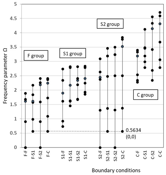
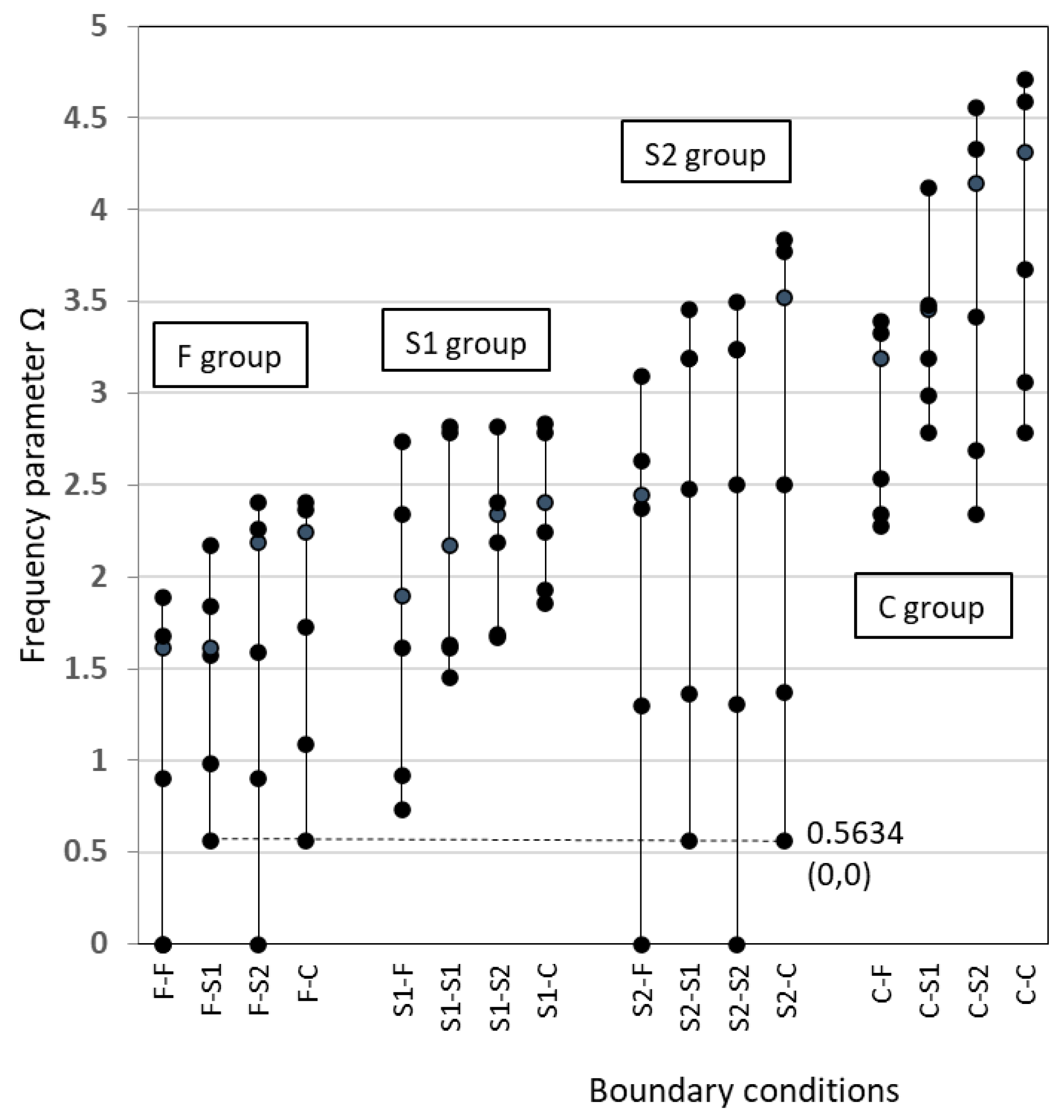
As is commonly seen in Table 3, Table 4, Table 5, Table 6, Table 7, Table 8, Table 9, Table 10, Table 11, Table 12, Table 13, Table 14, Table 15, Table 16, Table 17 and Table 18, the sequence of modes with increasing frequency values varies considerably depending on sets of boundary conditions on the outer and inner edges. It is seen that the lowest modes of F–F, F–S2, S2–F and S2–S2 show rigid body motion (i.e., the elastic frequency is zero), and that the lowest modes (n,s) = (0,0) of F–S1, F–C, S2–S1 and S2–C show identical frequencies, for example, Ω = 0.5634 for b/a = 0.3 (connected by a dotted line in Figure 3), because this mode shape yields practically the same kinematical constraints against a rotating mode shape, despite the superficial difference in the expression of the boundary condition. In Figure 3, the effects of using different boundary conditions are graphically summarized for an annular plate (b/a = 0.3, ν = 0.3). In the figure, all the frequencies are classified into four groups based on the outer edge condition (i.e., the outer edges are F, S-1, S-2 and C). Although these groups show a gradual increase in sets of frequencies in this order, there are a few observations that can be made, such as that the frequency gaps (differences) between Ω₁ and Ω₆ are relatively large for the F group and the S-2 group, and the gaps in the S1 group and the C group are relatively small (i.e., the frequencies are densely populated).

Figure 3. Distribution of the lowest six frequency parameters (including rigid body motions) of annular plates (b/a = 0.3, ν = 0.3) versus sixteen pairs of boundary conditions along outer–inner edges.

4. Conclusions

The first objective of this paper was to propose an extension of the Ritz method using special polynomial displacement functions and to demonstrate its solution’s accuracy by developing a self-coded FEM program for comparison purposes. After establishing the solution’s accuracy, the second objective was to provide comprehensive lists of frequency parameters for isotropic annular plates covering all sixteen combinations of four different types of boundary conditions (free, S1-supported, S2-supported, and clamped) at each edge. A wide range of aspect ratios (inner radius/outer radius) was considered. Accordingly, sufficiently comprehensive data sets have been provided for design purposes, for example, of rotating machinery, piezoelectric disks, and railway components, and as reference information for future research. In particular, the effect of the boundary conditions at the outer edge was clarified through the classification of their in-plane frequencies into groups. Although the numerical results were limited to isotropic annular plates, the formulation can be directly extended, for example, to laminated composite plates by simply inserting the appropriate material constants and stacking sequence information.

References

- Leissa, A.W. Vibration of Plates (NASA SP-160); Reprinted in 1993 by the Acoustical Society of America; National Aeronautics and Space Administration: Washington, DC, USA, 1969.
- Vogel, S.M.; Skinner, D.W. Natural frequencies of transversely vibrating uniform annular plates. J. Appl. Mech. 1965, 32, 926–931. [Google Scholar] [CrossRef] [Scilit]
- Janiman, Y.; Singh, B. Free vibration of circular annular plate with different boundary conditions. Vibroeng. Procedia 2019, 29, 82–86. [Google Scholar] [CrossRef] [Scilit]
- Narita, Y. Accurate results by the Ritz method for free vibration of uniform annular plates. Constr. Technol. Archit. 2023, 7, 11–20. [Google Scholar]
- Irie, T.; Yamada, G.; Muramoto, Y. Natural frequencies of in-plane vibration of annular plates. J. Sound Vib. 1984, 97, 171–175. [Google Scholar] [CrossRef] [Scilit]
- Bashmal, S.; Bhat, R.; Rakheha, S. In-plane free vibration of circular annular disks. J. Sound Vib. 2009, 322, 216–226. [Google Scholar] [CrossRef] [Scilit]
- Ravari, R.K.; Forouzan, M.R. Frequency equations for the in-plane vibration of orthotropic circular annular plate. Arch. Appl. Mech. 2011, 81, 1307–1322. [Google Scholar] [CrossRef] [Scilit]
- Shi, X.; Shi, D.; Qin, Z.; Wang, Q. In-plane vibration analysis of annular plates with arbitrary boundary conditions. Sci. World J. 2014, 4, 653836. [Google Scholar] [CrossRef] [Scilit] [PubMed]
- Shi, D.; Shi, X.; Li, W.L.; Qin, Z. Free in-plane vibration analysis of annular plates with general boundary conditions. Key Eng. Mater. 2014, 572, 189–192. [Google Scholar] [CrossRef] [Scilit]
- Wang, Q.; Shi, D.; Liang, Q.; Aha, F. A unified solution for free in-plane vibration of orthotropic circular, annular and sector plates with general boundary conditions. Appl. Math. Model. 2016, 40, 9228–9253. [Google Scholar] [CrossRef] [Scilit]
- Lyu, P.; Du, J.; Wang, Y.; Liu, Z. Free in-plane vibration analysis of rotating annular panels with elastic boundary restraints. J. Sound Vib. 2019, 439, 434–456. [Google Scholar] [CrossRef] [Scilit]
- Guan, X.; Qin, B.; Zhong, R.; Wang, Q. A unified solution for in-plane vibration analysis of composite laminated sector and annular plate with elastic constraints. J. Low Freq. Noise Vib. Act. Control. 2021, 40, 1764–1779. [Google Scholar] [CrossRef] [Scilit]
- Lyu, P.; Chen, Q.; Ning, D.; Du, J.; Li, Z. Modeling and analysis of in-plane vibration of multiple spinning annular plates coupled by elastic points. Eur. J. Mech.-A/Solids 2025, 112, 105670. [Google Scholar] [CrossRef] [Scilit]
Disclaimer/Publisher’s Note: The statements, opinions and data contained in all publications are solely those of the individual author(s) and contributor(s) and not of MDPI and/or the editor(s). MDPI and/or the editor(s) disclaim responsibility for any injury to people or property resulting from any ideas, methods, instructions or products referred to in the content. |
© 2026 by the author. Licensee MDPI, Basel, Switzerland. This article is an open access article distributed under the terms and conditions of the Creative Commons Attribution (CC BY) license.