


Abstract
Understanding post-fire visible greenness change is important for assessing spatial heterogeneity in mountainous burned landscapes, but satellite observations often cannot capture local variation. This study developed a workflow using Unmanned Aerial Vehicle (UAV) Red–Green–Blue (RGB) imagery for RGB-interpreted burn severity classification and Green Leaf Index (GLI)-derived visible greenness change analysis three years after fire. The workflow integrated object-based Random Forest (RF) classification, bi-temporal GLI difference (GLI) detection, and terrain-stratified analysis under RGB-only conditions. Object-based multi-feature representation, including a 41-dimensional (41D) feature set of color, texture, and gradient metrics, supported local burn severity mapping, although performance gain over the 23-dimensional (23D) set was modest and not statistically significant. The burned area was dominated by high and moderate severity classes. GLI-derived analysis showed limited visible greenness increase (mean GLI = 0.0058), with slightly more than half of pixels being positive; high severity areas had higher GLI, while low severity areas showed limited or negative values. GLI also varied across terrain, being higher on steeper slopes, mid-to-upper elevations, and east-facing aspects. The workflow provides a practical local-scale approach for post-fire analysis using high-resolution UAV RGB imagery, with results interpreted as case-specific visible greenness patterns rather than comprehensive ecological recovery.
1. Introduction
Post-fire vegetation recovery is a key indicator of forest ecosystem responses and restoration processes [1,2]. In the early post-fire stage, visible greenness change reflects variations in canopy or surface greenness after wildfire disturbance and provides useful information on vegetation response patterns. However, visible greenness change represents only an observable component of post-fire recovery and does not capture the full spectrum of ecological recovery, which also includes vegetation structure, species composition, soil properties, and hydrological processes [3,4].
Burn severity and terrain characteristics are important factors influencing the spatial distribution of post-fire vegetation responses. Differences in fire intensity, residual vegetation, fuel conditions, and fire behavior, together with slope, elevation, and aspect, can create heterogeneous greenness response patterns across burned landscapes [5,6,7]. Understanding how these factors are associated with greenness variation is essential for interpreting post-fire vegetation dynamics in complex mountainous environments.
Remote sensing has been widely used for burned-area delineation, burn severity assessment, and post-fire vegetation monitoring [4,8]. Multispectral indices, such as the differenced Normalized Burn Ratio (dNBR) and Relative differenced Normalized Burn Ratio (RdNBR), use near-infrared (NIR) and shortwave-infrared (SWIR) information and have been widely applied to burn severity assessment [9,10]. Recent studies have also used dense satellite time series and machine learning methods to map burned areas, assess fire severity, and evaluate vegetation recovery over large spatial and temporal extents [2,11]. However, satellite-based observations may be limited in capturing small burned patches, irregular boundaries, and local heterogeneity in complex mountainous terrain. Unmanned Aerial Vehicle (UAV) imagery provides high spatial resolution and flexible local-scale acquisition, making it a useful data source for detailed post-fire assessment when field surveys or high-resolution multispectral data are unavailable [12,13].
UAV Red–Green–Blue (RGB) imagery offers low-cost, accessible, and high-resolution data for local burned-area observation. Recent UAV-based studies have shown that RGB and multispectral imagery can support burned area and burn severity classification, although RGB-only information remains more spectrally constrained than multispectral data [14]. RGB-derived vegetation indices, such as the Green Leaf Index (GLI), can be used to describe visible greenness changes when NIR and SWIR bands are unavailable [15]. Nevertheless, RGB imagery lacks the spectral information required by indices such as dNBR and RdNBR, and RGB-derived greenness metrics may be sensitive to illumination, shadows, exposed soil, residual char, seasonal background variation, and phenology [13,16,17]. Consequently, GLI-based temporal analysis is suitable for examining visible greenness change, but ecological interpretation should consider burn severity, terrain conditions, and image acquisition context.
Object-based image analysis can reduce pixel-level noise by grouping spatially coherent image objects, while machine learning methods such as Random Forest (RF) classifiers can integrate color, brightness, texture, shape, vegetation-related, and gradient features to improve classification under complex surface conditions [7,13,18]. In UAV RGB-based burn severity mapping, visual features such as color, brightness, residual vegetation, charring, ash cover, exposed soil, and texture are important cues for interpreting RGB-based severity patterns, particularly when multispectral or field-based measurements are unavailable. Therefore, data source characteristics and labeling criteria remain important considerations when interpreting UAV RGB-derived burn severity maps.
Although previous UAV and remote-sensing studies have demonstrated the utility of high-resolution imagery for burned-area detection, severity mapping, and vegetation monitoring [12,13,14,16], many studies focus on these components separately. Under RGB-only conditions, jointly analyzing RGB-interpreted burn severity, bi-temporal GLI-derived visible greenness change, and terrain-stratified spatial patterns within a unified workflow remains insufficiently explored.
To address this gap, this study develops an object-based UAV RGB workflow that integrates multi-feature burn severity classification, bi-temporal GLI change detection, and terrain-stratified analysis. A 41-dimensional (41D) feature set characterizes burned objects in terms of color, vegetation-related, texture, shape, and gradient features. RGB-interpreted burn severity maps are generated using a Random Forest classifier, and GLI differences between two UAV observation periods are used to quantify early visible greenness change approximately three years post-fire. Spatial patterns of GLI change are analyzed across burn severity classes and terrain gradients.
This study is guided by three hypotheses: (1) object-based multi-feature representation can support consistent RGB-interpreted burn severity classification from UAV imagery; (2) early GLI-derived visible greenness change differs among burn severity classes due to varying initial disturbance conditions; and (3) terrain gradients, including slope, elevation, and aspect, are associated with spatial variability in early visible greenness change. Testing these hypotheses allows an assessment of the potential and limitations of UAV RGB imagery for post-fire visible greenness analysis.
2. Materials and Methods
2.1. Study Area
The study area is located in Jiangchuan District, Yuxi City, Yunnan Province, China (24°12′–24°32′ N, 102°35′–102°55′ E; Figure 1a–c). Jiangchuan District lies in the mountainous region of central Yunnan, where topographic variation is pronounced, and land cover is spatially heterogeneous. Forest is the dominant land-cover type, mainly composed of subtropical montane forest and secondary vegetation, with coniferous and mixed forest patches distributed across different slopes and elevations. These terrain and vegetation conditions provide a heterogeneous environmental background for fire effects and post-fire vegetation responses.
Figure 1.
Geographic location of the study area and Unmanned Aerial Vehicle (UAV) orthophotos of the extracted burned area. (a) Location of Yunnan Province in China; (b) location of Jiangchuan District in Yunnan Province; (c) location of the study area in Jiangchuan District; (d) extracted burned-area orthophoto in March 2023; (e) extracted burned-area orthophoto in February 2026.
A forest fire occurred in this region in March 2023. A representative fire-affected area of approximately 599 ha was selected as the study site, within which the burned area was delineated from the immediate post-fire UAV RGB orthophoto and used as the analysis domain (Figure 1d). The extracted burned area covered approximately 233 ha and contained heterogeneous patches characterized by surface charring, residual vegetation, exposed soil, and varying canopy greenness. All subsequent burn severity classification and greenness change analyses were conducted within this extracted burned-area boundary.
Post-fire greenness change can be influenced by vegetation composition, pre-fire stand conditions, rainfall variability, drought stress, natural regeneration, and restoration activities. However, systematic field measurements of species composition, soil properties, regeneration density, and management interventions were not available across the entire burned area. Based on available field observations and visual inspection of the UAV orthophotos, no large-scale artificial restoration or uniform management intervention was identified within the extracted burned area during the observation period. Therefore, this study focused on UAV RGB-derived visible greenness change rather than comprehensive ecological recovery, analyzing the observed changes as image-derived vegetation responses under the combined influence of burn severity, terrain conditions, and post-fire environmental background.
2.2. UAV Data Acquisition and Preprocessing
Low-altitude UAV RGB imagery was acquired using a DJI Matrice 4 Series unmanned aerial vehicle (SZ DJI Technology Co., Ltd., Shenzhen, China) over the same fire-affected area in March 2023 and February 2026. The March 2023 imagery was used as the immediate post-fire baseline, whereas the February 2026 imagery represented the early post-fire observation stage approximately three years after the fire (Figure 1d,e). Both surveys were conducted under favorable weather conditions, with no precipitation and low wind, to reduce image blurring and improve photogrammetric reconstruction quality. The flight altitude was approximately 150 m and was adjusted according to local terrain conditions to maintain image coverage over the mountainous area. The UAV images were accompanied by position and orientation system (POS) records, including image identifiers, acquisition timestamps, geographic coordinates, ellipsoidal heights, and positioning quality information.
Image processing was performed using Pix4Dmapper (version 4.4.12, Pix4D SA, Prilly, Switzerland). The UAV images and corresponding POS data were processed through aerial triangulation, image matching, bundle block adjustment, dense reconstruction, orthorectification, and mosaicking to generate RGB orthophotos for the two observation periods. For the February 2026 dataset, 409 RGB images were processed, and all images were successfully calibrated and geolocated. The camera model was M4T_6.7_4032x3024 (RGB). The generated orthomosaic had an average ground sampling distance (GSD) of 6.95 cm/pixel and covered approximately 0.879 km2 (87.89 ha). The dataset contained a median of 47,703 key points per image and 25,701 matched key points per calibrated image, with a mean reprojection error of 0.203 pixels. The orthomosaic was generated at 1 × GSD resolution, most pixels were covered by more than five overlapping images, and the output coordinate system was WGS84/UTM zone 48N.
In ArcGIS Pro (version 3.0.1, Esri, Redlands, CA, USA), the March 2023 orthophoto was used as the spatial reference to co-register and align the February 2026 orthophoto. The co-registered orthophotos were then clipped to the extracted burned-area boundary to ensure consistent spatial coverage and pixel correspondence. Because the analysis was based on RGB orthophotos acquired on different dates, the images were not treated as physically calibrated surface reflectance data. Color balancing was not applied during orthomosaic generation, and no reflectance map was generated. To reduce cross-date inconsistencies, the two orthophotos were processed within the same spatial extent and analyzed using the normalized RGB-based Green Leaf Index (GLI), which uses the relative relationship among the red, green, and blue channels and can reduce the influence of overall brightness differences to some extent.
GLI was calculated for both orthophotos, and the temporal difference between the two observation periods was used to characterize early post-fire visible greenness change. Pixels outside the extracted burned area were excluded, and the GLI change analysis was conducted only within the burned-area mask. Therefore, the resulting GLI difference (GLI) was used as an image-derived relative greenness change indicator under RGB-only data conditions.
Topographic variables were derived from the Shuttle Radar Topography Mission (SRTM) digital elevation model (DEM), provided by NASA and distributed through the USGS data archive. The DEM had a spatial resolution of approximately 30 m, with elevation values expressed in meters, and its reported absolute vertical accuracy is approximately 16 m at 90% confidence according to the SRTM product specification. The original DEM tiles were mosaicked, projected to the same coordinate reference system as the UAV orthophotos, clipped to the extracted burned area, and then resampled and aligned with the UAV-derived analysis layers in ArcGIS Pro. Slope, elevation, and aspect were then calculated within the burned area. Because the SRTM DEM was coarser than the UAV RGB orthophotos, the derived topographic variables were used for terrain stratification and statistical analysis rather than for interpreting centimeter-scale terrain variation. These variables, together with the burn severity classification results and greenness change metrics, were analyzed under a unified spatial framework.
2.3. Burned Area Delineation
The burned-area boundary was derived from the immediate post-fire UAV RGB orthophoto acquired in March 2023. Because the UAV imagery contained only visible RGB bands, NIR- or SWIR-based indices such as dNBR and RdNBR could not be calculated. Therefore, an RGB image-based binary semantic segmentation workflow was used to delineate burned and unburned surfaces.
The post-fire orthophoto was divided into image patches and input into a trained semantic segmentation model to generate a pixel-level burned area mask. The initial mask was post-processed by removing isolated noise, filling small holes, and refining fragmented boundaries, and was then converted into a vector boundary.
To ensure the reliability of the analysis mask, the model-derived boundary was visually checked against the original UAV orthophoto, and obvious non-burned patches, artifacts, and boundary inconsistencies were manually corrected. The final burned area covered approximately 233 ha and was used as the spatial mask for subsequent burn severity classification, topographic stratification, and greenness change assessment.
2.4. Burn Severity Classification Methodology
2.4.1. RGB-Interpreted Burn Severity Classification Criteria
Within the extracted burned area, burn severity was classified into three ordinal levels: low severity, moderate severity, and high severity, corresponding to Classes 1, 2, and 3, respectively. The classification scheme was adapted to the information available from high-resolution UAV RGB orthophotos and was based on visible-band characteristics, including color tone, brightness, residual vegetation, charring, ash cover, exposed soil or surface materials, and texture. These criteria were not intended to replace established field-based or multispectral burn severity assessment methods but were adapted from commonly used visual indicators of post-fire surface effects under RGB-only UAV image conditions.
The use of these visual indicators is supported by existing burn severity and soil burn severity studies. In soil burn severity mapping, ash cover, exposed mineral soil, charred materials, vegetation consumption, and surface color changes are commonly used to distinguish different severity levels [19]. The Composite Burn Index (CBI) also evaluates fire effects through visual ordinal assessments of vegetation strata, surface fuels, substrate conditions, and overall post-fire appearance [20]. In addition, white ash cover has been shown to be closely related to surface fuel consumption, supporting the use of ash cover or ash deposition as an indicator of surface fire effects [21]. Post-fire ash can also be detected by ground, UAV, and satellite observations, although its persistence may vary over time [22]. UAV-based studies have further shown that very high-resolution color orthomosaics can be used to extract burn severity-related surface metrics, such as residual green vegetation and charred organic surface [23]. Therefore, the selected RGB-observable indicators were considered suitable for object-level visual interpretation of burn severity in this study.
Because the UAV imagery did not contain NIR or SWIR bands, spectral burn indices such as the differenced Normalized Burn Ratio (dNBR) and Relative differenced Normalized Burn Ratio (RdNBR) were not calculated. In addition, systematic field-based soil burn severity (SBS) or CBI measurements were not available for independent validation. Therefore, the severity classes in this study were defined as RGB-interpreted burn severity classes derived from UAV-visible surface characteristics rather than field-validated ecological burn severity classes.
The interpretation criteria were established using visually observable post-fire surface characteristics. Low severity areas were characterized by limited visible fire effects, relatively abundant residual vegetation or green components, weak surface charring or ash cover, and heterogeneous vegetation texture. Moderate severity areas showed evident fire effects, including noticeable darkening or discoloration, partial charring, mixed burned and unburned patches, moderate ash cover or exposed surface materials, and heterogeneous transition textures. High severity areas were characterized by strong dark or ash-toned surfaces, extensive charring or ash deposition, high surface exposure, sparse vegetation remnants, and relatively homogeneous burned or exposed textures (Table 1).
Table 1.
Qualitative Red–Green–Blue (RGB)-interpreted burn severity criteria.
Labeling was conducted at the object level rather than directly at the pixel level. Superpixel segments within the burned area were used as the basic interpretation units, and each object was assigned a severity label according to its dominant visual characteristics. Objects located in severity transition zones were reviewed by comparing their color tone, brightness, charring degree, ash cover, residual vegetation, exposed surface materials, texture patterns, and local neighborhood context. The labeled objects were then used as reference samples for training and evaluating the object-based burn severity classifier.
2.4.2. Sample Construction and Data Partitioning
Object units within the burned area were manually labeled according to the predefined RGB-interpreted burn severity criteria to construct low-severity, moderate-severity, and high-severity samples. Three researchers participated in the annotation process. Before labeling, representative objects from different severity levels were jointly examined to calibrate the interpretation criteria. Ambiguous objects, including those located in severity transition zones or boundary areas, were reviewed by comparing their color tone, brightness, charring degree, ash cover, residual vegetation, exposed surface materials, texture patterns, and local neighborhood context. Final labels were assigned through consensus discussion.
Formal inter-annotator agreement statistics, such as Cohen’s kappa or Fleiss’s kappa, were not computed because the annotation was conducted as a consensus-based interpretation process rather than as fully independent labeling by multiple annotators. Complete independent label records for all objects were therefore not available. To reduce labeling subjectivity, predefined interpretation criteria, joint calibration, consensus review of ambiguous samples, and iterative inspection of classification results were adopted.
To improve the coverage of severity transition zones, complex boundary areas, and underrepresented classes, a multi-round iterative annotation and model training strategy was used. The dataset was progressively expanded through cycles of initial annotation, model training, result inspection, and targeted sample supplementation. During this process, low-severity objects and ambiguous transition objects were preferentially supplemented to improve sample coverage across severity classes.
After three rounds of annotation, the dataset expanded from 1278 to 2113 object samples, including 265 low-severity samples, 939 moderate-severity samples, and 909 high-severity samples (Table 2). The iterative sampling results did not show a monotonic improvement in validation accuracy. Accuracy increased from Round 1 (overall accuracy (OA) = 0.9313) to Round 2 (OA = 0.9338) but decreased in Round 3 (OA = 0.9237), while Ordered Mean Absolute Error (Ordered MAE) increased. This decrease was mainly related to the inclusion of more complex objects from transition zones, boundary areas, and underrepresented low severity patches. Therefore, Round 3 was retained because it provided broader sample coverage and better represented the spatial complexity of post-fire surfaces. The validation set was kept consistent across all sampling rounds to ensure the comparability of accuracy metrics.
Table 2.
Sample composition and model performance across iterative sampling rounds.
A group-based data partitioning strategy was applied to reduce spatial information leakage caused by adjacent object samples. Image tiles were used as grouping units, and a Group Shuffle Split scheme divided the dataset into training and validation sets at a ratio of 8:2. The same group-based splitting strategy and random seeds were used across the three sampling rounds. Performance metrics were reported as the average across 10 repeated splits. Class-sensitive metrics, including balanced accuracy, macro-F1 score, and class-wise precision, recall, and F1-score, were used to evaluate classification performance under class-imbalanced conditions.
An independent test set was further constructed for final model evaluation. Eight image tiles covering high-severity core areas, severity transition zones, and complex boundary regions were selected, yielding 237 object-level samples, including 29 low-severity samples, 123 moderate-severity samples, and 85 high-severity samples. This test set was excluded from training and validation and used only for final evaluation.
2.4.3. Feature Construction
To reduce the influence of local noise and fragmented boundaries in high-resolution UAV RGB imagery, an object-based classification strategy constrained by the burned-area mask was adopted. Superpixel segmentation was first performed within the burned area to generate homogeneous object units. The simple linear iterative clustering (SLIC) algorithm was used for object generation [24]. The burned-area image was processed using 1024 × 1024 pixel tiles. For each tile, the number of superpixels was set to 800, the compactness parameter to 15, and the Gaussian smoothing parameter to . Objects smaller than 30 pixels were removed or merged into adjacent objects to reduce isolated fragments. These settings were used to balance boundary adherence and object compactness while preserving local burn-severity transitions.
Object-level features were extracted to characterize post-fire surface variations, including color, brightness, texture, shape, vegetation-related color indices, and gradient information. Pixel-level values within each object were summarized mainly using the mean and standard deviation. To evaluate the effect of feature combinations on classification performance, two feature sets were constructed by adapting commonly used RGB color, color-space, vegetation-index, texture, shape, and gradient descriptors from image classification and remote sensing studies: a 23-dimensional (23D) basic feature set and a 41Dextended feature set.
The 23D feature set included RGB, Hue–Saturation–Value (HSV) [25], International Commission on Illumination (CIE) Lab [26], grayscale, texture, and shape features. RGB and grayscale statistics describe object-level color and brightness differences. HSV features characterize hue, saturation, and value variations, whereas CIE Lab features represent perceptual lightness and chromatic contrasts among burned surfaces, ash-covered areas, exposed soil, and vegetation remnants. Texture features based on the absolute Laplacian response reflect local surface roughness and structural heterogeneity, and object area was included as a shape descriptor.
The 41D feature set further incorporated normalized color components, visible-band vegetation indices, color-structure descriptors, and gradient response features (Table 3). The normalized RGB components, including , , and , were calculated using Equation (1) to reduce the influence of overall brightness differences and emphasize the relative contribution of each visible channel. The visible-band vegetation indices included Excess Green (ExG), Visible Atmospherically Resistant Index (VARI), and Normalized Green–Red Difference Index (NGRDI). ExG was calculated using Equation (2) and has been widely used to enhance green vegetation signals relative to soil and residue backgrounds [27]. VARI was calculated using Equation (3) and was designed to estimate green vegetation fraction using visible bands while reducing atmospheric sensitivity [28]. NGRDI was calculated using Equation (4) and describes the normalized contrast between green and red reflectance in RGB imagery [29]. Chroma and HueAB were derived from the CIE Lab color space using Equations (5) and (6), respectively, to describe chromatic strength and hue direction [26]. Sobel horizontal and vertical gradient responses were calculated using Equation (7), and Sobel gradient magnitude was calculated using Equation (8) to capture edge strength, boundary variation, and local structural changes. Such gradient-based descriptors have been applied in remote sensing image feature extraction [30,31].
Table 3.
Composition of the 23-dimensional (23D) and 41-dimensional (41D) feature sets.
The main extended features were calculated as follows:
where R, G, and B denote the red, green, and blue channel values, respectively; a and b are the chromatic components in the CIE Lab color space; I denotes the grayscale image; and are the horizontal and vertical Sobel kernels; and are the corresponding horizontal and vertical gradient responses; and ∗ denotes convolution. In implementation, a small constant was added to denominators where necessary to avoid division by zero.
2.4.4. Model Construction
For burn severity classification, four machine learning models were employed: Random Forest (RF), Extreme Gradient Boosting (XGBoost), Support Vector Machine (SVM), and Logistic Regression (LR). These models were selected for their complementary ability to capture nonlinear relationships and handle high-dimensional feature spaces.
To ensure consistency and comparability across experiments, commonly adopted parameter settings were used. No systematic hyperparameter optimization was performed, and other parameters were kept at default unless otherwise specified. Key settings were: RF with 300 trees, SVM with a radial basis function (RBF) kernel, LR with L2 regularization, and XGBoost with maximum tree depth of 6. Based on the optimal classifier–feature set combination identified through subsequent evaluation, the trained model was applied to the entire burned area to generate burn severity maps, distinguishing low-, moderate-, and high-severity classes.
2.4.5. Experimental Design and Evaluation Strategy
Model performance was evaluated through repeated validation, independent testing, and patch-level analysis. The experimental design aimed to assess the effect of iterative sample refinement and to compare different feature sets and classifiers under consistent evaluation criteria.
Four metrics were used for quantitative evaluation, including Balanced Accuracy (BA), Macro F1-score, OA, and Ordered MAE, as defined in Equations (9)–(13). BA measures the average recall across all classes:
where C is the number of classes, and denotes the recall of class i. The class-wise F1-score and Macro F1-score are defined in Equations (10) and (11):
where and are the precision and recall of class i, respectively. OA is calculated as the proportion of correctly classified samples, as shown in Equation (12):
where N is the total number of samples, and and denote the ground-truth and predicted labels, respectively. Considering the ordinal nature of burn severity, Ordered MAE was further used to measure the magnitude of classification errors across severity levels, as defined in Equation (13):
BA and Macro-F1 reflect class-wise performance balance, OA measures overall classification accuracy, and Ordered MAE evaluates the severity-level distance of misclassification.
To formally compare the 23D-RF and 41D-RF models, a paired Wilcoxon signed-rank test was applied to the performance metrics obtained from the 10 repeated group-based validation splits. The same Group Shuffle Split partitions and random seeds were used for both feature sets to ensure paired comparison. The tested metrics included OA, BA, Macro-F1, Weighted-F1, Ordered MAE, Within-1 rate, and severe misclassification rate. The Wilcoxon signed-rank test was selected because the validation results were paired and the number of repeated splits was limited. A significance level of was used.
To evaluate the contribution of sample refinement, the 23D basic feature set combined with RF was used as a consistent baseline across all sampling rounds. This configuration provided a stable reference for comparing the effects of iterative sample construction.
Patch-level analysis was further conducted to examine model performance in challenging areas, such as severity transition zones and complex background regions. For the optimal model, feature contribution analysis was also performed to identify the roles of color, brightness, texture, and extended features in burn severity discrimination.
2.5. Visible Greenness Change Analysis in the Forest Burned Area
2.5.1. Construction of the GLI-Based Greenness Change Metric
To characterize early visible greenness change within the burned area, the Green Leaf Index (GLI) [32] was calculated from the bi-temporal UAV RGB orthophotos. GLI is an RGB-derived vegetation index that reflects visible greenness using the relative relationship among the red, green, and blue channels. In this study, it was used as an image-derived greenness indicator rather than a direct measure of comprehensive ecological recovery, as defined in Equation (14):
where R, G, and B denote the pixel values of the red, green, and blue channels, respectively. Higher GLI values generally indicate stronger visible green vegetation components, whereas lower values are commonly associated with bare soil, charred surfaces, ash-covered areas, or low-greenness conditions.
To describe temporal greenness change between the two observation periods, the GLI difference (GLI) was calculated as Equation (15):
where and denote the GLI values in the first and second periods, respectively. Positive GLI values indicate an increase in visible greenness, whereas negative values indicate a decrease in visible greenness between the two periods.
Because the analysis was based on RGB orthophotos acquired on different dates, GLI was interpreted as an image-derived relative greenness change indicator. The analysis focused on spatial patterns and group-level differences across burn severity and terrain classes, rather than treating small pixel-level GLI values as direct ecological recovery estimates.
2.5.2. Severity and Topography Stratified Analysis Strategy
Following burn severity classification, zonal statistical analysis was conducted using low-severity, moderate-severity, and high-severity zones as the basic units within the extracted burned area. For each severity class and for the entire burned area, GLI-derived greenness change metrics were calculated from the bi-temporal UAV RGB data, including mean GLI, mean GLI, median GLI, and the proportion of pixels with GLI > 0. These indicators were used to summarize visible greenness change patterns and to compare differences among RGB-interpreted burn severity classes.
To examine terrain-related variation in GLI-derived greenness change, slope, elevation, and aspect were incorporated as stratification factors. The burned area was divided into multiple classes for each topographic variable, and greenness change metrics were calculated within each terrain class and burn severity class. This stratified analysis provided a descriptive comparison of greenness change patterns under different combinations of burn severity and terrain conditions.
Because soil moisture, drainage, solar radiation, microclimate, and pre-fire vegetation composition were not explicitly measured, the terrain-related results were interpreted as associations between topographic classes and GLI-derived greenness change rather than as independent causal effects. The analysis was therefore designed to characterize spatial variation in greenness change across severity and terrain strata under the available UAV RGB and DEM data conditions.
3. Results
3.1. Burn Severity Classification and Spatial Patterns
3.1.1. Burn Severity Classification via RF with 41D Features
- (1)
- Model Comparisons of 23D and 41D Feature Sets
The classification performance of different feature sets and models was compared during the model selection stage (Table 4). These values represent average validation results obtained from repeated group-based train–validation partitions. Among the tested classifiers, RF achieved the highest average validation performance under both the 23D and 41D feature sets and was therefore selected for subsequent independent evaluation and spatial mapping.
Table 4.
Classification performance of different feature sets and models.
Compared with the 23D feature set, the 41D feature set yielded slightly higher RF performance in the validation-based comparison, with OA increasing from 0.9237 to 0.9265 and Ordered MAE decreasing from 0.0811 to 0.0776. To formally examine whether this improvement was statistically significant, a paired Wilcoxon signed-rank test was conducted using the 10 repeated group-based validation results of the 23D-RF and 41D-RF models. The 41D-RF model showed slightly higher mean OA, BA, Macro-F1, and Weighted-F1 values and a slightly lower Ordered MAE than the 23D-RF model; however, none of these differences reached statistical significance at the 0.05 level (Table 5). Therefore, the 41D feature set was interpreted as providing supplementary object-level descriptive information rather than a statistically significant improvement in classification performance. The 41D feature set was retained for final mapping because it showed the highest average validation performance and included additional color, vegetation-related, structural, and gradient information relevant to burned-object discrimination.
Table 5.
Paired Wilcoxon signed-rank test results for 23D-RF and 41D-RF.
After model selection, the RF models using the 23D and 41D feature sets were further evaluated on the independent test set (Table 6). On that test set, the 41D-RF model showed slightly higher descriptive values than the 23D-RF model across all reported metrics, achieving an OA of 0.9367, a BA of 0.9318, a Macro-F1 of 0.9387, a Weighted-F1 of 0.9368, and an Ordered MAE of 0.0633. Both feature sets achieved a Within-1 rate of one and a severe misclassification rate of zero, indicating that misclassifications occurred only between adjacent severity levels. Overall, the 41D-RF model provided a modest descriptive advantage in the present dataset and was therefore used for final burn severity mapping.
Table 6.
RF performance with 23D and 41D feature sets on the independent test set.
The confusion matrices on the independent test set (Figure 2) show that misclassifications mainly occurred between the moderate severity and high severity classes. With the 41D feature set, the proportion of moderate severity objects misclassified as high severity decreased from 0.098 to 0.089, while the reverse misclassification rate decreased from 0.024 to 0.012. These results indicate that the 41D feature set reduced adjacent-class confusion to a limited extent near the moderate–high severity boundary. The remaining confusion was mainly concentrated between neighboring ordinal classes, which is consistent with the gradual transition of visible surface characteristics, including charring, ash cover, exposed soil, and residual vegetation, across severity levels.
Figure 2.
Row-normalized confusion matrices for the 23D-RF and 41D-RF models on the independent test set.
The burn severity maps generated by the 23D-RF and 41D-RF models showed broadly consistent spatial patterns, with high-severity areas dominating the extracted burned area and moderate-severity patches mainly distributed along local transition zones and less severely affected surfaces (Figure 3a,b). In the detailed views, the 41D-RF result showed more coherent high-severity patches and fewer fragmented moderate-severity pixels than the 23D-RF result, especially around road edges and local transition areas (Figure 3c,d). These map-level characteristics were consistent with the metric-based comparison and supported the use of the 41D-RF model for final spatial mapping under the present dataset, although the paired validation test indicated that the performance improvement was not statistically significant.
Figure 3.
Burn severity maps generated by (a) 23D-RF and (b) 41D-RF, with detailed views shown in (c,d).
- (2)
- Feature Contribution Analysis Based on SHAP
Shapley Additive Explanations (SHAP) analysis was used to evaluate the relative contribution of object-level features to the RF classification results, and the top 15 features were ranked according to their mean absolute SHAP values (Figure 4), including HueAB_mean, gN_mean, a_mean, H_mean, b_mean, ExG_mean, bN_mean, b_std, gN_std, NGRDI_mean, N_mean, VARI_mean, ExG_std, bN_std, and H_std. Most of these features are related to hue, normalized color composition, visible-band vegetation indices, and color variability, indicating that burn severity discrimination from UAV RGB imagery is strongly associated with object-level color appearance.
Figure 4.
Feature importance ranking based on mean absolute SHAP values (top 15).
The dominance of color- and hue-related features is consistent with the visual characteristics of burned surfaces. Low-severity areas usually retain more residual vegetation or green components, resulting in stronger green-channel contributions and higher greenness-related index values. In contrast, high-severity areas are commonly characterized by stronger charring, ash deposition, greater surface exposure, and fewer vegetation remnants, producing darker, ash-toned, or less green color responses. Moderate-severity areas often contain mixed burned and unburned components, leading to transitional color patterns. Therefore, features such as gN_mean, ExG_mean, NGRDI_mean, and VARI_mean reflect residual greenness, whereas HueAB_mean, H_mean, a_mean, and b_mean capture hue shifts and chromatic contrasts among charred surfaces, ash-covered areas, exposed soil, and vegetation remnants.
Variability-related features, including b_std, gN_std, ExG_std, bN_std, and H_std, further describe within-object heterogeneity. These features are particularly useful in severity transition zones, where burned surfaces, residual vegetation, ash cover, and exposed soil may coexist within the same object. Their contribution indicates that the RF model used not only mean color differences but also internal color variability associated with mixed burn conditions.
Overall, the SHAP results suggest that the 41D feature set provides complementary information by combining basic color statistics, normalized color components, visible-band vegetation indices, hue descriptors, and variability measures. These results help explain why the 41D feature set was retained for subsequent independent evaluation and spatial mapping from the perspective of feature interpretability. However, as shown by the paired Wilcoxon signed-rank test, the numerical improvement of 41D-RF over 23D-RF should be interpreted as modest and not statistically significant.
3.1.2. Spatial Patterns of Burn Severity
Based on the final burn severity classification results derived from the 41D-RF model, which was retained for mapping due to its highest average validation performance and complementary feature representation, area statistics indicate that high severity dominates the burned area, accounting for 60.17% (140.16 ha), followed by moderate severity at 37.54% (87.44 ha), while low severity comprises only 2.29% (5.33 ha) (Table 7).
Table 7.
Area statistics of different burn severity levels.
Spatially, burn severity does not exhibit a simple gradient pattern but instead shows a heterogeneous and mosaic-like distribution, with different severity levels interspersed across the burned area (Figure 5). High-severity areas are mainly concentrated in the central and southern parts, forming relatively large and continuous patches. Moderate-severity areas are primarily distributed in the surrounding regions and internal transition zones. Low-severity areas occur as fragmented patches along the fire perimeter and within localized areas.
Figure 5.
Spatial distribution of burn severity derived from the 41D-RF model.
3.2. Visible Greenness Change in the Forest Burned Area
3.2.1. GLI-Derived Visible Greenness Change
- (1)
- GLI-Derived Visible Greenness Change in the Whole Area
The early visible greenness change of the burned area was analyzed using GLI maps from two periods and their corresponding GLI (Figure 6). Here, visible greenness change refers to GLI-derived relative changes in visible vegetation greenness between the two UAV observation periods, rather than direct estimates of comprehensive ecological recovery. The GLI map was used as a descriptive indicator of relative spatial change patterns, not as a pixel-wise statistical significance map.
Figure 6.
Spatial distribution of GLI in (a) 2023 and (b) 2026, and (c) the GLI between the two periods. The GLI map describes relative spatial patterns of RGB-derived visible greenness change rather than pixel-wise statistical significance.
Overall, the burned area showed a slight increase in GLI-derived visible greenness three years after the fire. In the first period, GLI values were relatively low and spatially homogeneous, reflecting substantial loss of visible greenness immediately after the fire (Figure 6a). In the second period, GLI showed more pronounced spatial differentiation, with patchy increases in visible greenness in parts of the burned area, although low-GLI regions remained widespread (Figure 6b).
The GLI map shows that positive values were more widely distributed than negative values, suggesting a general but weak increase in visible greenness across the burned area (Figure 6c). However, areas with relatively high GLI were interspersed with regions showing little change or negative GLI, indicating a fragmented and spatially heterogeneous change pattern. Therefore, the GLI results should be interpreted as relative RGB-derived greenness change patterns rather than as evidence of statistically significant recovery or degradation at the pixel level.
- (2)
- Statistical Testing of Group Differences in GLI
To evaluate whether the descriptive differences in GLI among burn severity and terrain classes were statistically supported, Kruskal–Wallis tests were conducted using grid-level GLI values. Significant overall differences were detected for RGB-interpreted burn severity, slope, elevation, and aspect classes (Table 8). Dunn post hoc tests with Benjamini–Hochberg correction were further used to identify pairwise differences. The statistical results provide group-level support for differences in GLI-derived visible greenness change among severity and terrain classes.
Table 8.
Kruskal–Wallis test results for grid-level GLI across grouping factors.
- (3)
- GLI-Derived Visible Greenness Change across Different Burn Severity Classes
GLI-derived visible greenness change varied among RGB-interpreted burn severity classes (Figure 7). For the whole burned area, the mean GLI was 0.0058 and the median was 0.0015, indicating a limited overall increase in visible greenness with substantial spatial variability. The low-severity class showed a decrease in visible greenness, with a mean GLI of and a median of , and only 25.49% of pixels exhibited positive GLI. The moderate-severity class showed a weak increase in visible greenness, with a mean GLI of 0.0043 and a slightly negative median (), indicating considerable internal heterogeneity; 49.07% of pixels showed a positive GLI. The high-severity class showed the highest mean positive GLI value, with a mean GLI of 0.0086, a median of 0.0035, and 54.23% of pixels exhibiting positive values.
Figure 7.
Comparison of GLI among RGB-interpreted burn severity classes.
The Kruskal–Wallis test indicated a significant overall difference in grid-level GLI among RGB-interpreted burn severity classes (, ). Dunn’s post hoc comparisons with Benjamini–Hochberg correction showed that pairwise differences among low-severity, moderate-severity, and high-severity classes did not reach significance after correction (). Together, the descriptive statistics and statistical test indicate an overall severity-related difference in GLI-derived visible greenness change, with low-severity areas showing negative GLI and high-severity areas showing the largest positive mean GLI.
The relatively higher GLI observed in high-severity areas may be partly related to the very low initial GLI baseline immediately after severe burning, when strong charring, ash cover, and vegetation loss substantially reduced visible greenness. Under such conditions, even limited post-fire surface greening can produce a relatively large positive GLI. During the second UAV survey, surface greening was visually observed in some high-severity patches, mainly in the form of low vegetation cover or shrub-like regrowth. These observations were consistent with the spatial pattern of positive GLI in high-severity areas, but no systematic plot-based field survey was conducted in this study.
Overall, GLI-derived visible greenness change showed severity-related variation at the group level, and topographic factors were further associated with the spatial variability of GLI, as examined in the next section.
3.2.2. GLI-Derived Visible Greenness Change in Relation to Topographic Factors
To examine how early visible greenness change varied under different topographic conditions, UAV RGB-derived GLI was further summarized by slope, elevation, and aspect classes. This terrain-stratified analysis provided the basis for comparing GLI-derived visible greenness change across individual topographic factors and their combinations with RGB-interpreted burn severity. The GLI used in this analysis reflects relative visible-greenness changes derived from RGB imagery rather than direct measurements of vegetation biomass or physiological recovery (Figure 8, Figure 9, Figure 10, Figure 11, Figure 12 and Figure 13).
Figure 8.
Variation in GLI-derived visible greenness change (GLI) across slope classes.
Figure 9.
Mean GLI across RGB-interpreted burn severity and slope classes.
Figure 10.
Variation in GLI-derived visible greenness change (GLI) across elevation classes.
Figure 11.
Mean GLI across elevation classes for different RGB-interpreted burn severity classes.
Figure 12.
Variation in GLI-derived visible greenness change (GLI) across aspect classes.
Figure 13.
Mean GLI across aspect classes for different RGB-interpreted burn severity classes.
- (1)
- GLI-Derived Visible Greenness Change across Slope Classes
GLI increased with slope class (Figure 8). The median GLI rose from 0.0016 in the 0–5° class to 0.0219 in the >25° class, and the proportion of pixels with positive GLI increased from 57.03% to 86.25%. The boxplot distributions also showed greater variability and higher upper ranges in steeper classes, indicating higher local GLI-derived greenness change in steep terrain.
The Kruskal–Wallis test showed significant differences in grid-level GLI among slope classes (, ). Dunn’s post hoc comparisons indicated that the >25° class differed significantly from the 0–5°, 5–15°, and 15–25° classes. The 0–5° and 15–25° classes also showed a significant difference, whereas the differences between 0–5° and 5–15°, and between 5–15° and 15–25°, were not significant after correction. These results show that the steepest slope class had a distinct GLI distribution, consistent with the higher GLI-derived greenness change observed in descriptive statistics.
This slope-related pattern may be associated with differences in post-fire surface conditions and early vegetation establishment. Steeper slopes in the study area were often characterized by more exposed surfaces and lower retained vegetation cover immediately after the fire, resulting in a lower initial greenness baseline. Under such conditions, early colonization by herbaceous vegetation or shrub-like regrowth can produce a relatively clear increase in RGB-derived greenness. In addition, slope-related drainage and microhabitat differences may contribute to spatial variation in GLI-derived greenness change. Overall, the slope-stratified GLI distribution showed an increasing trend with slope, with the steepest class differing most clearly from the other slope classes.
When burn severity was considered together with slope, GLI showed different patterns across slope classes (Figure 9). On gentle slopes (0–5°), low-severity areas showed negative GLI (), whereas moderate-severity and high-severity areas showed positive values. As slope increased, GLI generally rose across severity levels, and the differences among severity classes became smaller. On the steepest slopes (>25°), GLI values across severity levels converged around 0.021–0.022, suggesting a more uniform GLI-derived greenness change pattern under steep-slope conditions.
The convergence of GLI among severity classes on steep slopes indicates reduced severity-related differences in early GLI-derived greenness change under steep-slope conditions. In these areas, the combined presence of low initial greenness, exposed post-fire surfaces, and early surface vegetation development may reduce the apparent contrast among severity classes. In steep terrain, local GLI variation was more pronounced and accompanied by higher spatial heterogeneity.
Overall, GLI patterns varied across slope classes, with values tending to converge among severity classes on steeper slopes. These results indicate slope-related differences in GLI-derived visible greenness change.
- (2)
- GLI-Derived Visible Greenness Change across Elevation Classes
GLI showed a non-linear pattern across elevation classes (Figure 10). The mean GLI increased from in the low-elevation class to 0.0088 in the upper-middle-elevation class and then decreased slightly to 0.0063 at high elevations. The proportion of pixels with positive GLI followed a similar trend, increasing from 50.93% at low elevations to 67.93% in the upper-middle-elevation class, before decreasing to 59.70% at high elevations. These results indicate that GLI-derived greenness change showed relatively higher positive values in the upper-middle elevation range. Median GLI showed a broadly similar pattern, although localized areas with higher positive GLI were also observed at high elevations.
The Kruskal–Wallis test indicated significant differences in grid-level GLI among elevation classes (, ). Dunn’s post hoc comparisons showed significant pairwise differences among all elevation classes after correction, including comparisons involving the upper-middle-elevation class. These statistical results support the observed non-linear elevation pattern and show that the upper-middle-elevation class had a distinct GLI distribution compared with the other elevation strata.
The elevation-related pattern may reflect the combined influence of local temperature, moisture availability, solar radiation, and vegetation establishment conditions. Low-elevation areas may be more strongly affected by human disturbance, exposed surfaces, or drier post-fire conditions, limiting visible greenness increase in some locations. In contrast, upper-middle elevations may provide relatively favorable microclimatic conditions for early vegetation regrowth, with moderate temperature and moisture conditions supporting herbaceous colonization or shrub resprouting. At higher elevations, lower temperature, thinner soils, or stronger exposure may partially limit further increases in visible greenness, leading to a slight decline from the upper-middle-elevation peak.
When burn severity was included, the relationship between elevation and GLI differed among severity levels (Figure 11). At low elevations, moderate-severity areas showed negative GLI (), whereas low-severity and high-severity areas showed slightly positive values. As elevation increased, GLI generally increased across all severity levels and peaked in the upper-middle-elevation class. In that class, high-severity areas reached the highest mean GLI (0.0100), followed by moderate-severity and low-severity areas. At high elevations, GLI remained positive for all severity levels but decreased slightly from the upper-middle peak.
This pattern shows that the relationship between RGB-interpreted burn severity and GLI-derived greenness change differed across elevation classes. The relatively higher GLI in high-severity areas at upper-middle elevations may be related to the combination of a low post-fire greenness baseline and favorable microenvironmental conditions for early surface vegetation development. Thus, the spatial distribution of GLI was associated with both elevation strata and RGB-interpreted burn severity classes.
Overall, GLI varied across elevation classes, with the clearest positive values observed in the upper-middle-elevation class. Severity-related differences also differed among elevation classes, indicating that GLI-derived visible greenness change was associated with both RGB-interpreted burn severity and elevation strata.
- (3)
- GLI-Derived Visible Greenness Change across Aspect Classes
GLI varied among aspect classes (Figure 12). East-facing areas showed the highest mean GLI (0.0094), followed by south-facing (0.0046) and north-facing areas (0.0041). Flat and west-facing areas showed lower mean values, at 0.0015 and 0.0037, respectively. Median GLI showed a similar pattern, with east-facing areas remaining relatively high (0.0074). The proportion of positive GLI pixels also varied among aspect classes, with east-facing areas showing the highest proportion (67.27%), while north-facing and west-facing areas showed lower proportions of 57.02% and 57.64%, respectively.
The relatively higher GLI on east-facing slopes may be related to aspect-driven differences in solar radiation, moisture retention, and thermal stress. East-facing slopes receive more direct radiation in the morning, which may provide favorable light conditions while avoiding stronger afternoon heat and moisture stress that can occur on west-facing slopes. North-facing slopes may receive lower radiation and experience cooler or more humid microconditions, whereas south-facing slopes may be exposed to stronger solar radiation. These aspect-dependent microclimatic differences may be associated with early vegetation establishment and surface greenness after fire. In addition, aspect can affect illumination conditions in UAV RGB imagery, and local shadow differences may contribute to variation in GLI values, particularly in complex mountainous terrain.
When burn severity was considered together with aspect, differences among aspect classes became more complex (Figure 13). East-facing areas showed relatively high GLI under moderate and high severity, with high-severity areas reaching 0.0097, while low-severity areas were slightly negative. Flat areas showed strong variation, with high-severity areas showing negative GLI (). North-facing areas showed a decreasing trend from low to high severity, with relatively higher GLI under low severity and lower values under moderate and high severity. South-facing areas remained positive across all severity levels, with the highest GLI under low severity. West-facing areas showed contrasting behavior, with negative GLI under low severity () and positive values under moderate and high severity.
These aspect-related differences indicate that severity-related patterns of GLI-derived greenness change varied across aspect classes. The relatively high GLI in east-facing moderate-severity and high-severity areas may be associated with more favorable aspect conditions for early surface greening after severe disturbance. In contrast, the more variable patterns in flat and west-facing areas may reflect mixed land-surface conditions, local shading, and greater heterogeneity in post-fire vegetation development.
Overall, GLI varied among aspect classes, with east facing slopes showing relatively higher positive values. Flat and west-facing areas exhibited more variable patterns, and severity-related differences also changed across aspect classes. These results indicate that GLI-derived visible greenness change showed terrain-related variation across slope, elevation, and aspect strata.
4. Discussion
4.1. Main Findings and Comparison with Previous Studies
This study used UAV RGB imagery to classify RGB-interpreted burn severity and analyze early GLI-derived visible greenness change in a mountainous burned forest area. The use of UAV imagery is consistent with previous studies showing that very high resolution UAV data can support fine-scale burn severity classification and post-fire damage assessment [14,33]. Compared with basic RGB color features, the 41D feature set provided modest numerical improvements by incorporating object color, structure, texture, and gradient information. Similar findings have also been reported in high-resolution burn severity mapping studies, where multi-feature representations improved the characterization of heterogeneous fire effects [34].
However, the improvement from 23D-RF to 41D-RF was numerically small, and the paired Wilcoxon signed-rank test indicated that the differences were not statistically significant for the evaluated metrics. This suggests that the additional features in the 41D feature set provided supplementary object-level descriptive information but did not lead to a statistically robust improvement in classification performance under the current repeated validation setting. Moderate- and high-severity classes were partially confused, reflecting the continuous transition of surface charring, ash cover, exposed soil, and residual vegetation in boundary zones. Such ambiguity is common in burn severity assessment because fire effects often vary gradually rather than forming completely discrete classes [35,36]. High-severity areas were mainly concentrated in the central and southern parts of the burned area, possibly due to fuel continuity, slope, topography, and local wind. These factors may influence fire behavior, but without detailed measurements, these explanations remain plausible interpretations. Low-severity areas were sparse, which limited the interpretability of their corresponding GLI statistics.
GLI-derived metrics showed a slight increase in visible greenness approximately three years after fire disturbance, with a mean GLI of 0.0058 and 51.64% positive pixels. Because GLI is calculated from visible RGB bands, it should be interpreted as an image-derived indicator of visible greenness rather than a direct measure of vegetation physiology or comprehensive ecological recovery [32,37]. The relatively higher GLI values in high-severity areas were mainly associated with lower initial GLI baselines, rather than necessarily indicating faster ecological recovery. Such early greening in high-severity areas may reflect opportunistic herbaceous colonization, shrub resprouting, or low vegetation regrowth rather than recovery of forest canopy structure or mature forest vegetation. In contrast, low-severity areas showed negative GLI values, likely because they had higher initial green cover immediately after fire.
Terrain-stratified analysis showed that GLI generally increased with slope and reached relatively high values at middle-to-upper elevations and east-facing aspects. These patterns are broadly consistent with previous post-fire recovery studies showing that topography, climate, and burn severity jointly regulate vegetation recovery trajectories [38,39]. Nevertheless, these results should be interpreted as spatial associations rather than independent causal effects, because key environmental drivers such as species composition, soil properties, rainfall variation, drought stress, and management interventions were not systematically measured in this study.
4.2. Methodological Implications and Limitations
The main methodological contribution of this study is the integration of object-based burn severity mapping, bi-temporal GLI analysis, and terrain-stratified comparison within a unified RGB-only UAV workflow. The use of UAV imagery provides very high resolution spatial information for fine-scale post-fire assessment, which has been increasingly applied in burned-area and burn severity studies [33]. GLI was selected as a simple and interpretable visible-greenness indicator suitable under RGB-only conditions, using the relative relationship among red, green, and blue channels to describe visible vegetation when NIR or SWIR bands were unavailable [37].
However, GLI has clear spectral and radiometric limitations. As an RGB-derived vegetation index, it cannot capture canopy water content, vegetation structure, char-related SWIR responses, soil burn effects, or below-canopy recovery, and therefore cannot replace indices such as the Normalized Difference Vegetation Index (NDVI), dNBR, or RdNBR [39,40]. In addition, GLI may be influenced by illumination differences, terrain shadows, viewing-angle effects, potential geometric distortion in steep terrain, exposed soil, ash and char backgrounds, sensor exposure, and seasonal phenology. These uncertainties are particularly relevant because the observed mean GLI was small and the two UAV acquisitions were conducted in different months [41,42]. No sensitivity analysis or ecological significance threshold was applied; therefore, the reported GLI differences should be interpreted as image-derived visible greenness differences rather than validated ecological recovery thresholds. In addition, the GLI map does not provide pixel-wise uncertainty estimates or statistical significance information. As a result, the spatial patterns shown in the GLI map should be regarded as descriptive RGB-derived visible greenness change patterns, rather than statistically significant recovery or degradation at the pixel level.
Burn severity classification relied on RGB visual interpretation without independent field-based validation, such as CBI or SBS assessment. Visual observations and UAV image inspections were used only as ancillary interpretation support rather than systematic plot-based validation. CBI assesses fire effects on vegetation and soil, while SBS mapping evaluates post-fire soil conditions and erosion-related risks [19,39]. In addition, the RGB-interpreted labels were generated through a consensus-based visual interpretation process. Formal inter-annotator agreement statistics, such as Cohen’s kappa or Fleiss’s kappa, were not available because complete independent label records from the three researchers were not retained for all objects. Although predefined criteria, joint calibration, and consensus review were used to reduce labeling subjectivity, the lack of quantitative inter-annotator agreement assessment remains a limitation. The independent test set was also limited, especially for low-severity samples. Moderate–high-severity confusion and boundary uncertainty may therefore propagate into the severity-stratified GLI analysis. The 41D feature set improved object representation but yielded limited numerical gains, and the paired Wilcoxon signed-rank test indicated that these gains were not statistically significant. Therefore, the added features should be interpreted as supplementary rather than decisive.
Terrain-stratified GLI patterns, although statistically supported, are descriptive rather than causal because several key environmental factors were not directly measured, including soil moisture, wind exposure, fuel load, microclimate, species composition, and post-fire management. Previous studies have shown that post-fire vegetation recovery is jointly affected by burn severity, topography, climate, and land-cover conditions [39]. Therefore, the terrain-related patterns observed in this study should be regarded as spatial associations under RGB-only UAV observations rather than independent causal mechanisms. Because a multivariate statistical framework was not applied, the independent effects of burn severity, slope, elevation, and aspect could not be isolated.
4.3. Future Work and Practical Relevance
Despite these limitations, the workflow demonstrates that RGB-only UAV data can provide spatially detailed burn severity maps and early visible greenness patterns at local scales, supporting rapid assessment, field survey planning, and identification of severely affected areas. The use of UAVs and ultra-high-resolution imagery for post-fire vegetation dynamics monitoring has been highlighted in recent studies, including multi-temporal UAV workflows and integration with advanced processing techniques [43,44].
Future studies should integrate multi-temporal UAV observations, radiometric calibration panels, multispectral or hyperspectral imagery, light detection and ranging (LiDAR)-derived structural metrics, satellite-based dNBR/RdNBR products, and plot-based ecological measurements (e.g., CBI, SBS). Such multi-sensor integration has shown improved capability to disentangle radiometric artifacts from true vegetation dynamics and quantify structural versus spectral recovery signals [4,45]. Multi-sensor and multi-platform approaches have also been demonstrated to improve discrimination between canopy and understory recovery and to better link structural changes with spectral vegetation indicators [46].
Integrating field-based measurements with remote sensing products will also aid in validating RGB-interpreted severity classes and quantifying the contributions of burn severity, terrain, fuel, and environmental drivers to post-fire visible greenness changes. Comparisons with previous UAV and high-resolution studies indicate that, under more limited spectral conditions, RGB-only workflows can still achieve reasonable local classification performance while emphasizing the importance of multi-sensor validation and broader spatial replication [47,48].
5. Conclusions
This study developed a UAV RGB-based workflow for RGB-interpreted burn severity classification and GLI-derived early visible greenness change analysis in a mountainous forest burned area. The main contribution of this work does not lie in the individual use of UAV imagery for burn severity mapping or post-fire vegetation monitoring but in the integration of object-based RGB-interpreted burn severity classification, bi-temporal GLI-derived visible greenness change detection, and terrain-stratified spatial analysis within a unified RGB-only framework. Rather than replacing field-based burn severity assessment or multispectral remote sensing approaches, the proposed workflow provides a practical local-scale method for organizing high-resolution UAV RGB imagery into severity maps, visible greenness change outputs, and terrain-stratified spatial summaries when multispectral or field data are unavailable.
The results demonstrate the feasibility of using object-based multi-feature representation for RGB-interpreted burn severity mapping in the present case. The 41D feature set provided complementary information for representing burned-object color, texture, and gradient variation, although its improvement over the 23D feature set was modest and not statistically significant based on the paired Wilcoxon signed-rank test. Therefore, the added features should be interpreted as supplementary object-level descriptive information rather than as producing a statistically robust performance improvement. The remaining confusion between moderate-severity and high-severity classes indicates that adjacent RGB-interpreted severity levels remain difficult to separate in transition zones. The GLI-derived analysis showed only a slight overall increase in visible greenness approximately three years after fire. Among the RGB-interpreted burn severity classes, high-severity areas exhibited relatively higher GLI values, whereas low-severity areas showed limited or negative GLI. In addition, GLI varied across slope, elevation, and aspect strata, indicating terrain-related spatial heterogeneity in early visible greenness change within the study area.
Several limitations should be acknowledged. Burn severity classes were derived from RGB visual interpretation and were not independently validated using field CBI/SBS measurements or dNBR/RdNBR products. The GLI analysis was based on two UAV RGB orthophotos acquired in different months, without robust cross-date radiometric normalization, reflectance calibration, calibration panels, shadow masking, soil-background correction, or topographic illumination correction. Given the small magnitude of the observed GLI, part of the detected change may be affected by illumination, shadow, terrain effects, surface background, seasonal conditions, or phenological differences. In addition, the independent test set was limited in size, low-severity samples were relatively few, and the study focused on a single fire event. Future work should integrate multi-temporal UAV observations acquired at comparable phenological stages, multispectral or hyperspectral imagery, LiDAR-derived structural information, satellite dNBR/RdNBR products, and plot-based ecological measurements to validate RGB-interpreted severity classes, distinguish radiometric artifacts from true vegetation dynamics, and better quantify the relative roles of burn severity, terrain, fuel conditions, and environmental drivers in post-fire visible greenness change.
Author Contributions
Conceptualization, Q.G., C.X. and W.K.; methodology, Q.G., C.X. and Z.H.; software, Q.G.; validation, Q.G., C.X., W.K. and Z.H.; formal analysis, Q.G. and C.X.; investigation, Q.G., C.X. and J.Y.; resources, W.K., C.X. and Q.W.; data curation, Q.G., C.X. and J.Y.; writing—original draft preparation, Q.G. and C.X.; writing—review and editing, W.K., Z.H. and Q.W.; visualization, Q.G.; supervision, W.K. and Q.W.; project administration, W.K.; funding acquisition, W.K. All authors have read and agreed to the published version of the manuscript.
Funding
This research was funded by the National Natural Science Foundation of China, grant number 32260391; the Yunnan International Joint Laboratory of Natural Rubber Intelligent Monitoring and Digital Applications, grant number 202403AP140001; the Yunnan International Joint R&D Center (China–Malaysia) for Digital Monitoring, Management and Applications of Nature Reserves, grant number 202503AP140040; Yunnan Fundamental Research Projects, grant number 2018FG001-059; the Xingdian Talent Support Program, grant numbers XDYC-CYCX-2024-0021 and YFGRC202532; and the Academician Li Wei Workstation of Yunnan Province, grant number 202505AF350082; the Yunnan Province Expert Workstation of Chen Yong, grant number 202505AF350005.
Institutional Review Board Statement
Not applicable.
Informed Consent Statement
Not applicable.
Data Availability Statement
The data presented in this study are available from the corresponding author upon reasonable request.
Acknowledgments
The authors gratefully acknowledge the support provided by the Forestry and Grassland Bureau of Jiangchuan District, Yuxi, China, in fieldwork coordination and UAV image acquisition. The authors also gratefully acknowledge the support of Southwest Forestry University for this research.
Conflicts of Interest
The authors declare no conflicts of interest.
Abbreviations
The following abbreviations are used in this manuscript:
| UAV | Unmanned Aerial Vehicle |
| RGB | Red–Green–Blue |
| GLI | Green Leaf Index |
| SBS | Soil Burn Severity |
| RF | Random Forest |
| SVM | Support Vector Machine |
| RBF | Radial Basis Function |
| SHAP | SHapley Additive exPlanations |
| XGBoost | Extreme Gradient Boosting |
| dNBR | Differenced Normalized Burn Ratio |
| RdNBR | Relative Differenced Normalized Burn Ratio |
| 23D | 23-Dimensional Feature Set |
| 41D | 41-Dimensional Feature Set |
References
- Kuo, C.C.; Liu, Y.L.; Lin, C.T. Fine-scale post-fire forest recovery patterns and compound drivers in Taiwan’s high-mountain national parks. For. Ecol. Manag. 2026, 609, 123618. [Google Scholar] [CrossRef] [Scilit]
- Li, K.; Liu, Z.; Xu, W.; Wang, W.; Su, J.; Lv, Q.; Guo, W.; Johnson, M. Post-fire spectral recovery and driving factors across the boreal and temperate forests. Philos. Trans. R. Soc. B Biol. Sci. 2025, 380, 20230453. [Google Scholar] [CrossRef] [Scilit]
- Keeley, J.E. Fire intensity, fire severity and burn severity: A brief review and suggested usage. Int. J. Wildland Fire 2009, 18, 116–126. [Google Scholar] [CrossRef] [Scilit]
- Pérez-Cabello, F.; Montorio, R.; Alves, D.B. Remote sensing techniques to assess post-fire vegetation recovery. Curr. Opin. Environ. Sci. Health 2021, 21, 100251. [Google Scholar] [CrossRef] [Scilit]
- Cansler, C.A.; McKenzie, D. Climate, fire size, and biophysical setting control fire severity and spatial pattern in the northern Cascade Range, USA. Ecol. Appl. 2014, 24, 1037–1056. [Google Scholar] [CrossRef] [Scilit]
- Bradstock, R.A.; Hammill, K.A.; Collins, L.; Price, O. Effects of weather, fuel and terrain on fire severity in topographically diverse landscapes of south-eastern Australia. Landsc. Ecol. 2010, 25, 607–619. [Google Scholar] [CrossRef] [Scilit]
- Gao, J.; Chen, Y.; Xu, B.; Li, W.; Ye, J.; Kou, W.; Xu, W. Post-Fire Forest Ecological Quality Recovery Driven by Topographic Variation in Complex Plateau Regions: A 2006–2020 Landsat RSEI Time-Series Analysis. Forests 2025, 16, 502. [Google Scholar] [CrossRef] [Scilit]
- Kurbanov, E.; Vorobev, O.; Lezhnin, S.; Sha, J.; Wang, J.; Li, X.; Cole, J.; Dergunov, D.; Wang, Y. Remote Sensing of Forest Burnt Area, Burn Severity, and Post-Fire Recovery: A Review. Remote Sens. 2022, 14, 4714. [Google Scholar] [CrossRef] [Scilit]
- Miller, J.D.; Thode, A.E. Quantifying burn severity in a heterogeneous landscape with a relative version of the delta Normalized Burn Ratio (dNBR). Remote Sens. Environ. 2007, 109, 66–80. [Google Scholar] [CrossRef] [Scilit]
- Miller, J.D.; Knapp, E.E.; Key, C.H.; Skinner, C.N.; Isbell, C.J.; Creasy, R.M.; Sherlock, J.W. Calibration and validation of the relative differenced Normalized Burn Ratio (RdNBR) to three measures of fire severity in the Sierra Nevada and Klamath Mountains, California, USA. Remote Sens. Environ. 2009, 113, 645–656. [Google Scholar] [CrossRef] [Scilit]
- Chen, L.; Wei, B.; Jia, X.; Liu, M.; Zhao, Y. Burned Area Mapping and Fire Severity Assessment of Forest–Grassland Ecosystems Using Time-Series Landsat Imagery (1985–2023): A Case Study of Daxing’anling Region, China. Fire 2025, 8, 337. [Google Scholar] [CrossRef] [Scilit]
- Qarallah, B.; Al-Ajlouni, M.; Al-Awasi, A.; Alkarmy, M.; Al-Qudah, E.; Naser, A.B.; Al-Assaf, A.; Gevaert, C.M.; Al Asmar, Y.; Belgiu, M.; et al. Evaluating post-fire recovery of Latroon dry forest using Landsat ETM+, unmanned aerial vehicle and field survey data. J. Arid Environ. 2021, 193, 104587. [Google Scholar] [CrossRef] [Scilit]
- von Nonn, J.; Villarreal, M.L.; Blesius, L.; Davis, J.; Corbett, S. An open-source workflow for scaling burn severity metrics from drone to satellite to support post-fire watershed management. Environ. Model. Softw. 2024, 172, 105903. [Google Scholar] [CrossRef] [Scilit]
- Simes, T.; Pádua, L.; Moutinho, A. Wildfire Burnt Area Severity Classification from UAV-Based RGB and Multispectral Imagery. Remote Sens. 2024, 16, 30. [Google Scholar] [CrossRef] [Scilit]
- Chen, C.; Yuan, X.; Gan, S.; Luo, W.; Bi, R.; Li, R.; Gao, S. A new vegetation index based on UAV for extracting plateau vegetation information. Int. J. Appl. Earth Obs. Geoinf. 2024, 128, 103668. [Google Scholar] [CrossRef] [Scilit]
- Arnett, J.T.; Coops, N.C.; Daniels, L.D.; Falls, R.W. Detecting forest damage after a low-severity fire using remote sensing at multiple scales. Int. J. Appl. Earth Obs. Geoinf. 2015, 35, 239–246. [Google Scholar] [CrossRef] [Scilit]
- Peticilă, A.; Iliescu, P.G.; Dinca, L.; Popa, A.S.; Murariu, G. Vegetation Indices from UAV Imagery: Emerging Tools for Precision Agriculture and Forest Management. AgriEngineering 2025, 7, 431. [Google Scholar] [CrossRef] [Scilit]
- Gibson, R.; Danaher, T.; Hehir, W.; Collins, L. A remote sensing approach to mapping fire severity in south-eastern Australia using sentinel 2 and random forest. Remote Sens. Environ. 2020, 240, 111702. [Google Scholar] [CrossRef] [Scilit]
- Parsons, A.; Robichaud, P.R.; Lewis, S.A.; Napper, C.; Clark, J.T. Field Guide for Mapping Post-Fire Soil Burn Severity; Technical Report; U.S. Department of Agriculture, Forest Service, Rocky Mountain Research Station: Fort Collins, CO, USA, 2010. [CrossRef] [Scilit]
- Key, C.H.; Benson, N.C. Landscape Assessment (LA): Sampling and Analysis Methods; Technical Report RMRS-GTR-164-CD; U.S. Department of Agriculture, Forest Service, Rocky Mountain Research Station: Fort Collins, CO, USA, 2006.
- Hudak, A.T.; Ottmar, R.D.; Vihnanek, R.E.; Brewer, N.W.; Smith, A.M.S.; Morgan, P. The Relationship of Post-Fire White Ash Cover to Surface Fuel Consumption. Int. J. Wildland Fire 2013, 22, 780–785. [Google Scholar] [CrossRef] [Scilit]
- Lewis, S.A.; Robichaud, P.R.; Hudak, A.T.; Strand, E.K.; Eitel, J.U.H.; Brown, R.E. Evaluating the Persistence of Post-Wildfire Ash: A Multi-Platform Spatiotemporal Analysis. Fire 2021, 4, 68. [Google Scholar] [CrossRef] [Scilit]
- Fraser, R.H.; Van der Sluijs, J.; Hall, R.J. Calibrating Satellite-Based Indices of Burn Severity from UAV-Derived Metrics of a Burned Boreal Forest in NWT, Canada. Remote Sens. 2017, 9, 279. [Google Scholar] [CrossRef] [Scilit]
- Achanta, R.; Shaji, A.; Smith, K.; Lucchi, A.; Fua, P.; Süsstrunk, S. SLIC Superpixels Compared to State-of-the-Art Superpixel Methods. IEEE Trans. Pattern Anal. Mach. Intell. 2012, 34, 2274–2282. [Google Scholar] [CrossRef] [Scilit] [PubMed]
- Smith, A.R. Color gamut transform pairs. ACM Siggraph Comput. Graph. 1978, 12, 12–19. [Google Scholar] [CrossRef] [Scilit]
- McLaren, K. XIII—The Development of the CIE 1976 (L* a* b*) Uniform Colour Space and Colour-Difference Formula. J. Soc. Dye. Colour. 1976, 92, 338–341. [Google Scholar] [CrossRef] [Scilit]
- Woebbecke, D.M.; Meyer, G.E.; Bargen, K.V.; Mortensen, D.A. Color indices for weed identification under various soil, residue, and lighting conditions. Trans. ASABE 1994, 38, 259–269. [Google Scholar] [CrossRef] [Scilit]
- Gitelson, A.A.; Kaufman, Y.J.; Stark, R.; Rundquist, D. Novel algorithms for remote estimation of vegetation fraction. Remote Sens. Environ. 2002, 80, 76–87. [Google Scholar] [CrossRef] [Scilit]
- Hunt, E.R.; Cavigelli, M.; Daughtry, C.S.T.; McMurtrey, J.E.; Walthall, C.L. Evaluation of Digital Photography from Model Aircraft for Remote Sensing of Crop Biomass and Nitrogen Status. Precis. Agric. 2005, 6, 359–378. [Google Scholar] [CrossRef] [Scilit]
- Lacroix, V.; Acheroy, M. Feature extraction using the constrained gradient. ISPRS J. Photogramm. Remote Sens. 1998, 53, 85–94. [Google Scholar] [CrossRef] [Scilit]
- Hao, S.; Wu, B.; Zhao, K.; Ye, Y.; Wang, W. Two-Stream Swin Transformer with Differentiable Sobel Operator for Remote Sensing Image Classification. Remote Sens. 2022, 14, 1507. [Google Scholar] [CrossRef] [Scilit]
- Louhaichi, M.; Borman, M.M.; Johnson, D.E. Spatially located platform and aerial photography for documentation of grazing impacts on wheat. Geocarto Int. 2001, 16, 65–70. [Google Scholar] [CrossRef] [Scilit]
- Shin, J.I.; Seo, W.W.; Kim, T.; Park, J.; Woo, C.S. Using UAV Multispectral Images for Classification of Forest Burn Severity—A Case Study of the 2019 Gangneung Forest Fire. Forests 2019, 10, 1025. [Google Scholar] [CrossRef] [Scilit]
- Meng, R.; Wu, J.; Schwager, K.L.; Zhao, F.; Dennison, P.E.; Cook, B.D.; Brewster, K.; Green, T.M.; Serbin, S.P. Using high spatial resolution satellite imagery to map forest burn severity across spatial scales in a Pine Barrens ecosystem. Remote Sens. Environ. 2017, 191, 95–109. [Google Scholar] [CrossRef] [Scilit]
- Lentile, L.B.; Holden, Z.A.; Smith, A.M.S.; Falkowski, M.J.; Hudak, A.T.; Morgan, P.; Lewis, S.A.; Gessler, P.E.; Benson, N.C. Remote Sensing Techniques to Assess Active Fire Characteristics and Post-Fire Effects. Int. J. Wildland Fire 2006, 15, 319–345. [Google Scholar] [CrossRef] [Scilit]
- Whitman, E.; Parisien, M.A.; Thompson, D.K.; Flannigan, M.D. Topoedaphic and Forest Controls on Post-Fire Vegetation Assemblies Are Modified by Fire History and Burn Severity in the Northwestern Canadian Boreal Forest. Forests 2018, 9, 151. [Google Scholar] [CrossRef] [Scilit]
- Lussem, U.; Bolten, A.; Gnyp, M.L.; Jasper, J.D.; Bareth, G. Evaluation of RGB-based vegetation indices from UAV imagery to estimate forage yield in grassland. Int. Arch. Photogramm. Remote Sens. Spat. Inf. Sci. 2018, 42, 1215–1219. [Google Scholar] [CrossRef] [Scilit]
- Viana-Soto, A.; Aguado, I.; Martínez, S. Assessment of Post-Fire Vegetation Recovery Using Fire Severity and Geographical Data in the Mediterranean Region (Spain). Environments 2017, 4, 90. [Google Scholar] [CrossRef] [Scilit]
- Zahura, F.T.; Bisht, G.; Li, Z.; McKnight, S.; Chen, X. Impact of Topography and Climate on Post-Fire Vegetation Recovery across Different Burn Severity and Land Cover Types through Machine Learning. Ecol. Inform. 2024, 82, 102757. [Google Scholar] [CrossRef] [Scilit]
- Lee, S.H.; Lee, M.H.; Kang, T.H.; Cho, H.R.; Yun, H.S.; Lee, S.J. Comparative Analysis of dNBR, dNDVI, SVM Kernels, and ISODATA for Wildfire-Burned Area Mapping Using Sentinel-2 Imagery. Remote Sens. 2025, 17, 2196. [Google Scholar] [CrossRef] [Scilit]
- Barbier, N.; Ploton, P.; Tulet, H.; Viennois, G.; Leblanc, H.; Burban, B.; Réjou-Méchain, M.; Verley, P.; Ball, J.; Feurer, D.; et al. Monitoring tropical forests with light drones: Ensuring spatial and temporal consistency in stereophotogrammetric products. ISPRS Open J. Photogramm. Remote Sens. 2026, 19, 100114. [Google Scholar] [CrossRef] [Scilit]
- Rodrigo-Comino, J.; Gatea Al-Shammary, A.A.; Durán-Zuazo, V.H.; Serrano-Bernardo, F.; Caballero-Calvo, A.; Rodríguez-Galiano, V. The Limits of RGB-Based Vegetation Indexes under Canopy Degradation: Insights from UAV Monitoring of Harvested Cereal Fields. Drones Auton. Veh. 2026, 3, 10021. [Google Scholar] [CrossRef] [Scilit]
- Petrov, O.; Medvedev, A. Analyzing Post-fire Vegetation Dynamics with Ultra-high Resolution Remote Sensing Data. Int. Arch. Photogramm. Remote Sens. Spat. Inf. Sci. 2025, 48, 1189–1195. [Google Scholar] [CrossRef] [Scilit]
- Guiop-Servan, R.E.; Cotrina-Sanchez, A.; Puerta-Culqui, J.; Oliva-Cruz, M.; Barboza, E. Remote Sensing for Wildfire Mapping: A Comprehensive Review of Advances, Platforms, and Algorithms. Fire 2025, 8, 316. [Google Scholar] [CrossRef] [Scilit]
- Batchelor, J.L.; Hudak, A.T.; Kato, A.; Weise, D.R.; Moskal, L.M. Drone-based, multispectral photogrammetric point clouds to classify fire severity at differing canopy height strata. Fire Ecol. 2025, 21, 39. [Google Scholar] [CrossRef] [Scilit]
- Meng, R.; Wu, J.; Zhao, F.; Cook, B.D.; Hanavan, R.P.; Serbin, S.P. Measuring short-term post-fire forest recovery across a burn severity gradient in a mixed pine-oak forest using multi-sensor remote sensing techniques. Remote Sens. Environ. 2018, 210, 282–296. [Google Scholar] [CrossRef] [Scilit]
- Lazzeri, G.; Frodella, W.; Rossi, G.; Moretti, S. Multitemporal Mapping of Post-Fire Land Cover Using Multiplatform PRISMA Hyperspectral and Sentinel-UAV Multispectral Data: Insights from Case Studies in Portugal and Italy. Sensors 2021, 21, 3982. [Google Scholar] [CrossRef] [Scilit]
- Pádua, L.; Adão, T.; Guimarães, N.; Sousa, A.; Peres, E.; Sousa, J.J. Post-fire forestry recovery monitoring using high-resolution multispectral imagery from unmanned aerial vehicles. Int. Arch. Photogramm. Remote Sens. Spat. Inf. Sci. 2019, 42, 301–305. [Google Scholar] [CrossRef] [Scilit]
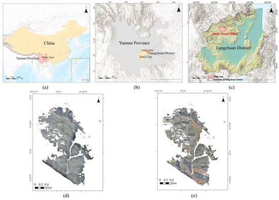
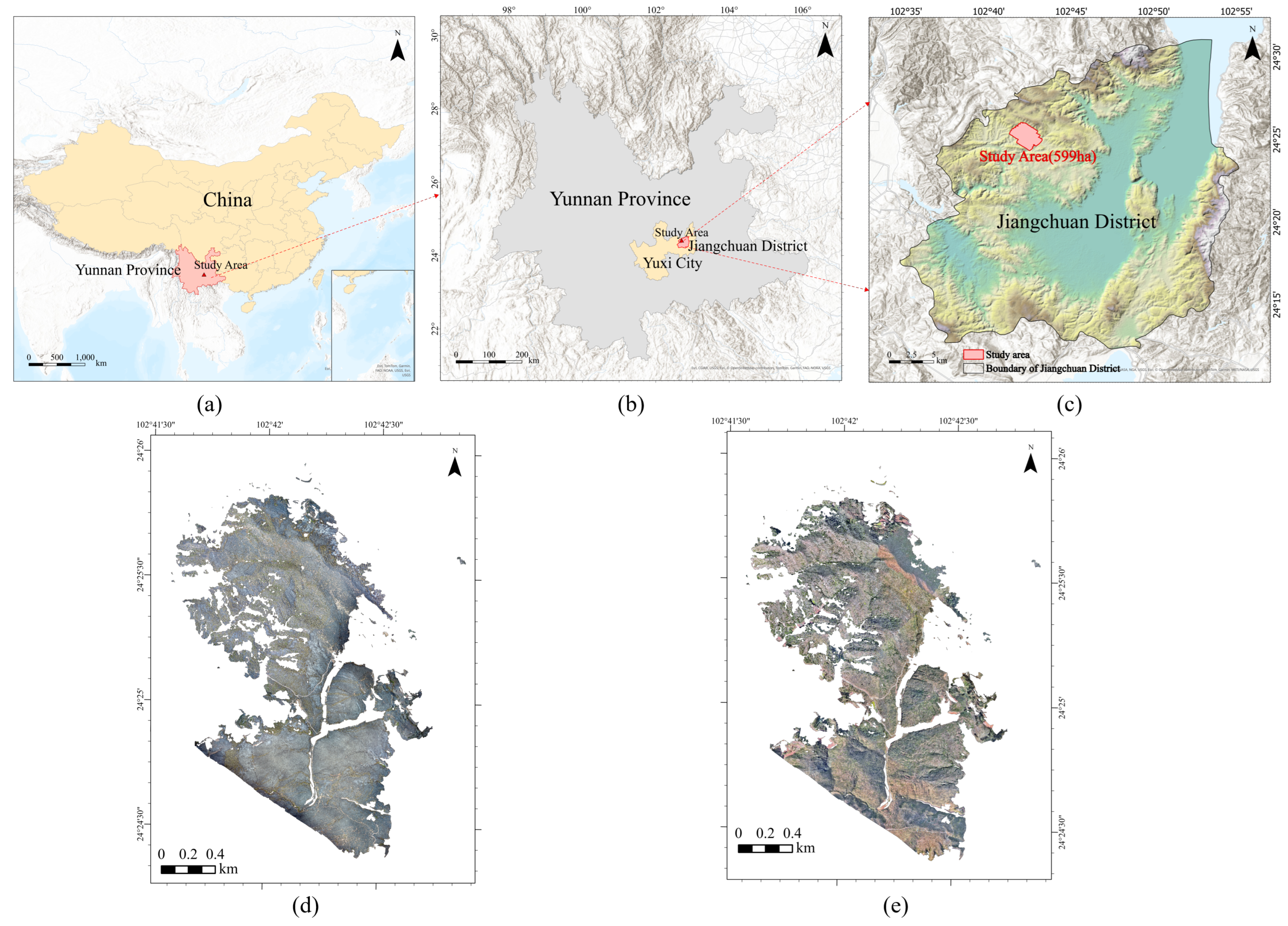
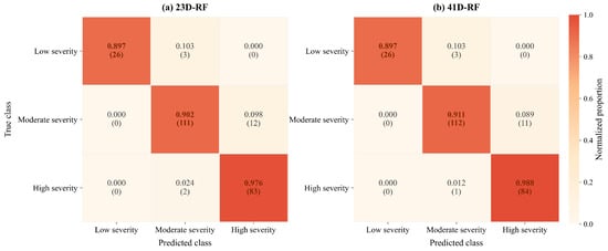
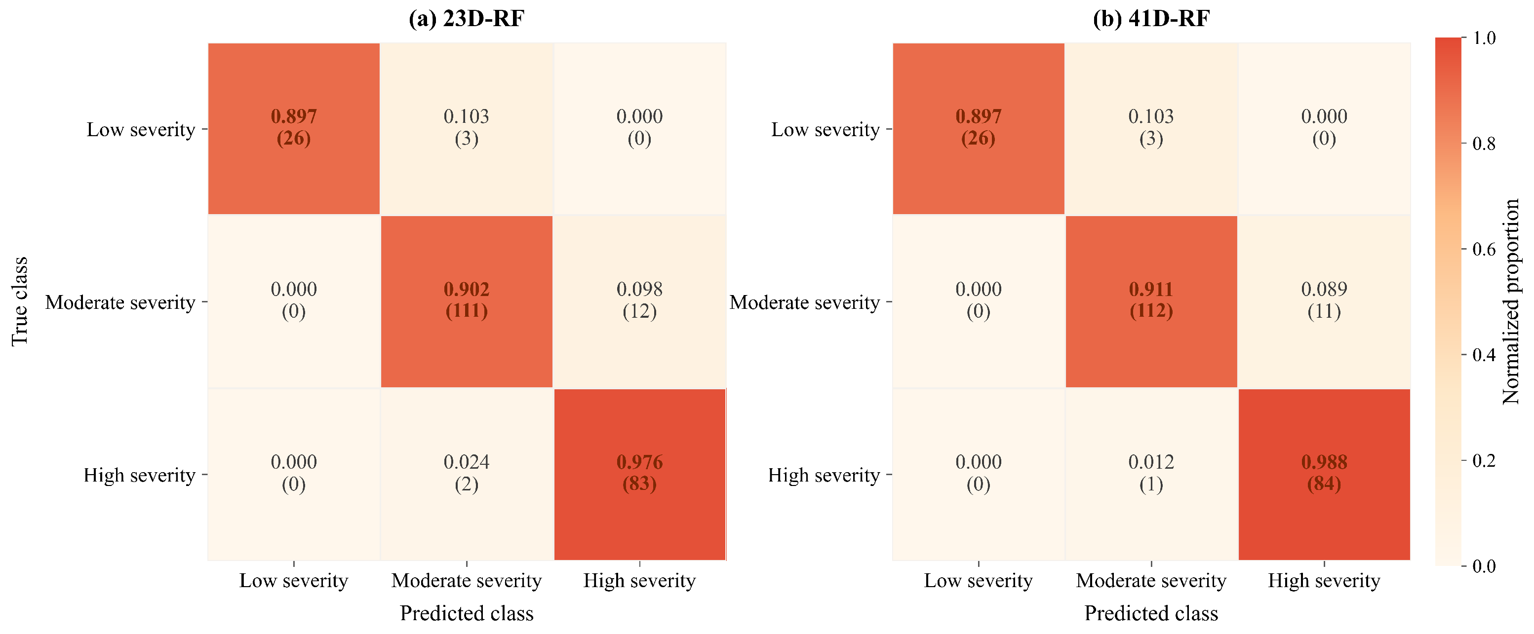
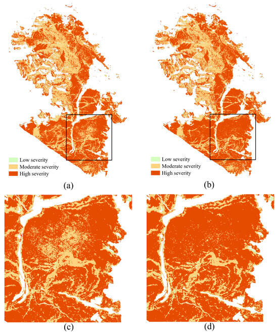
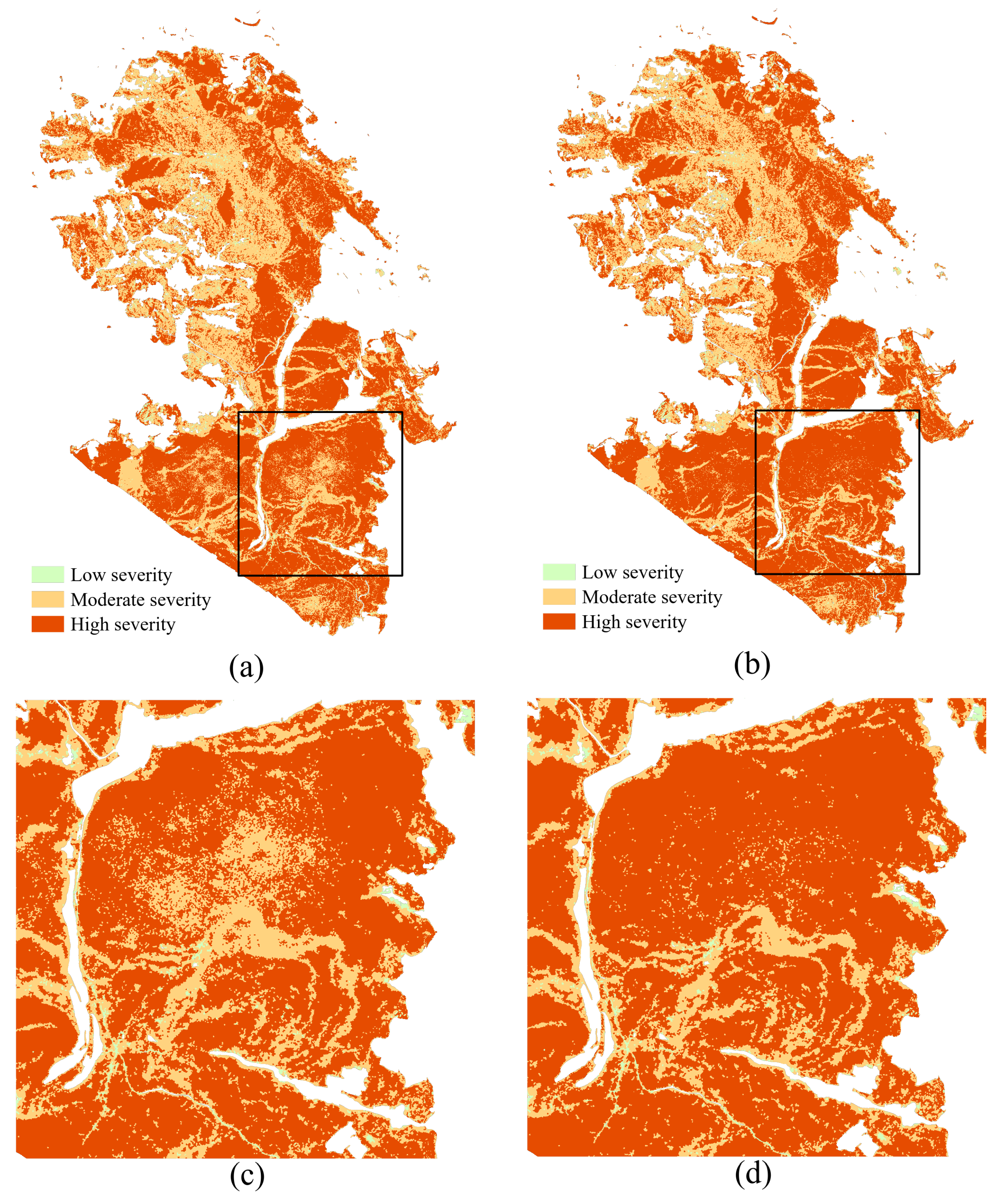
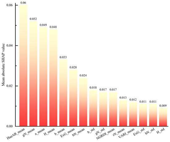
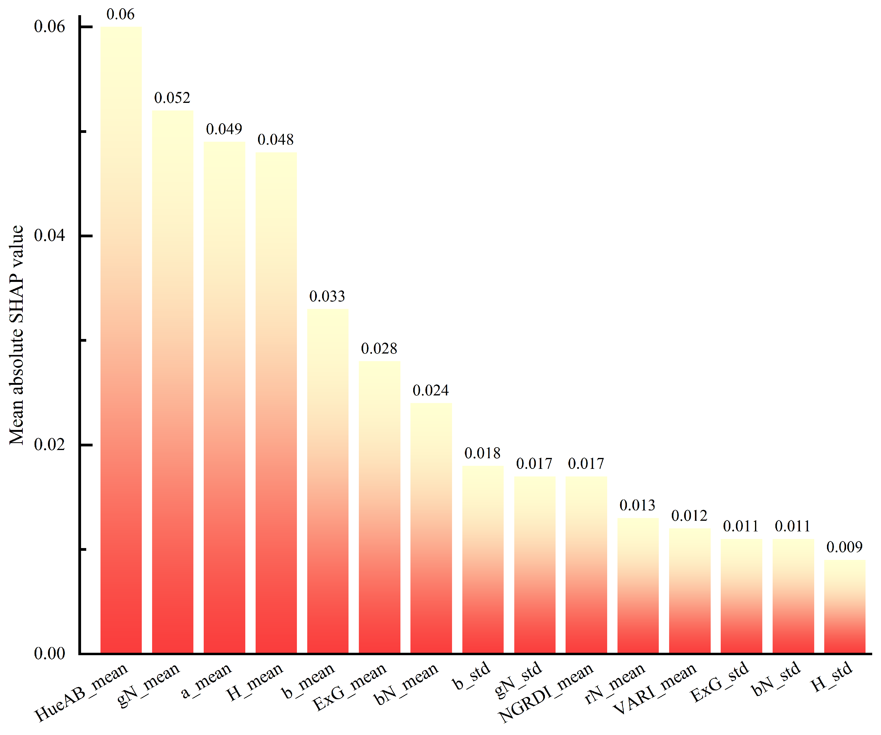
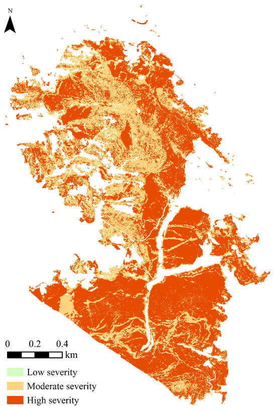
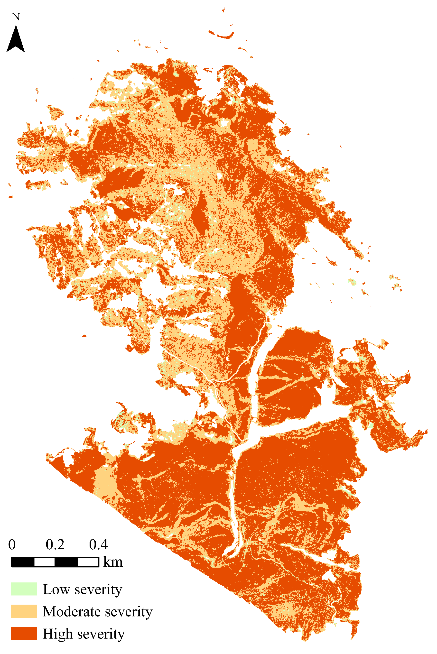
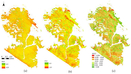
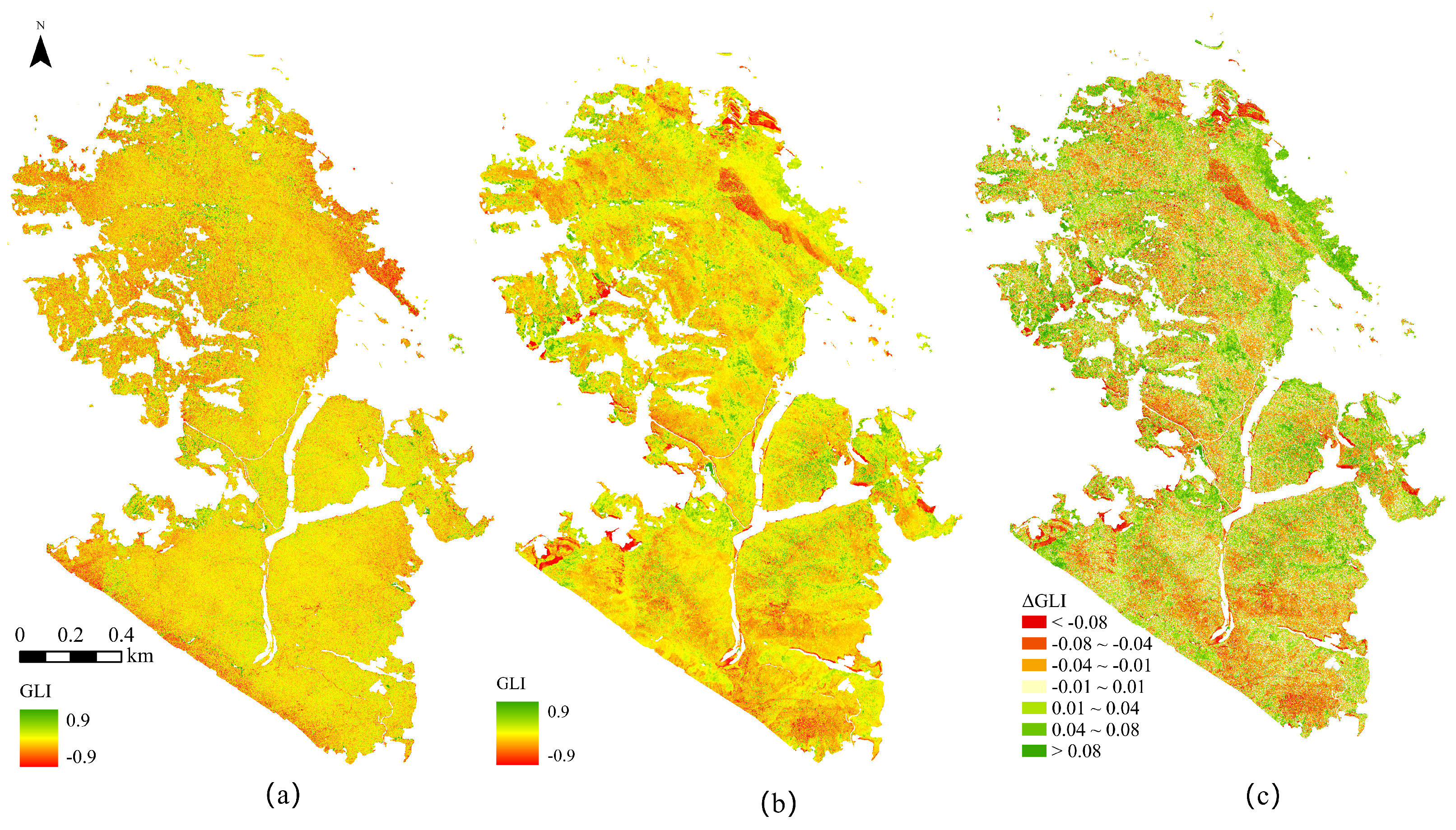
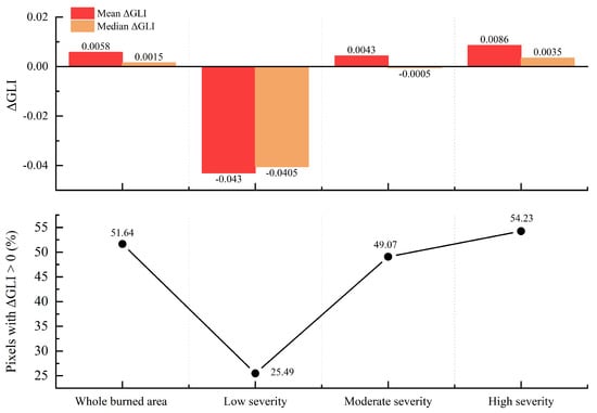
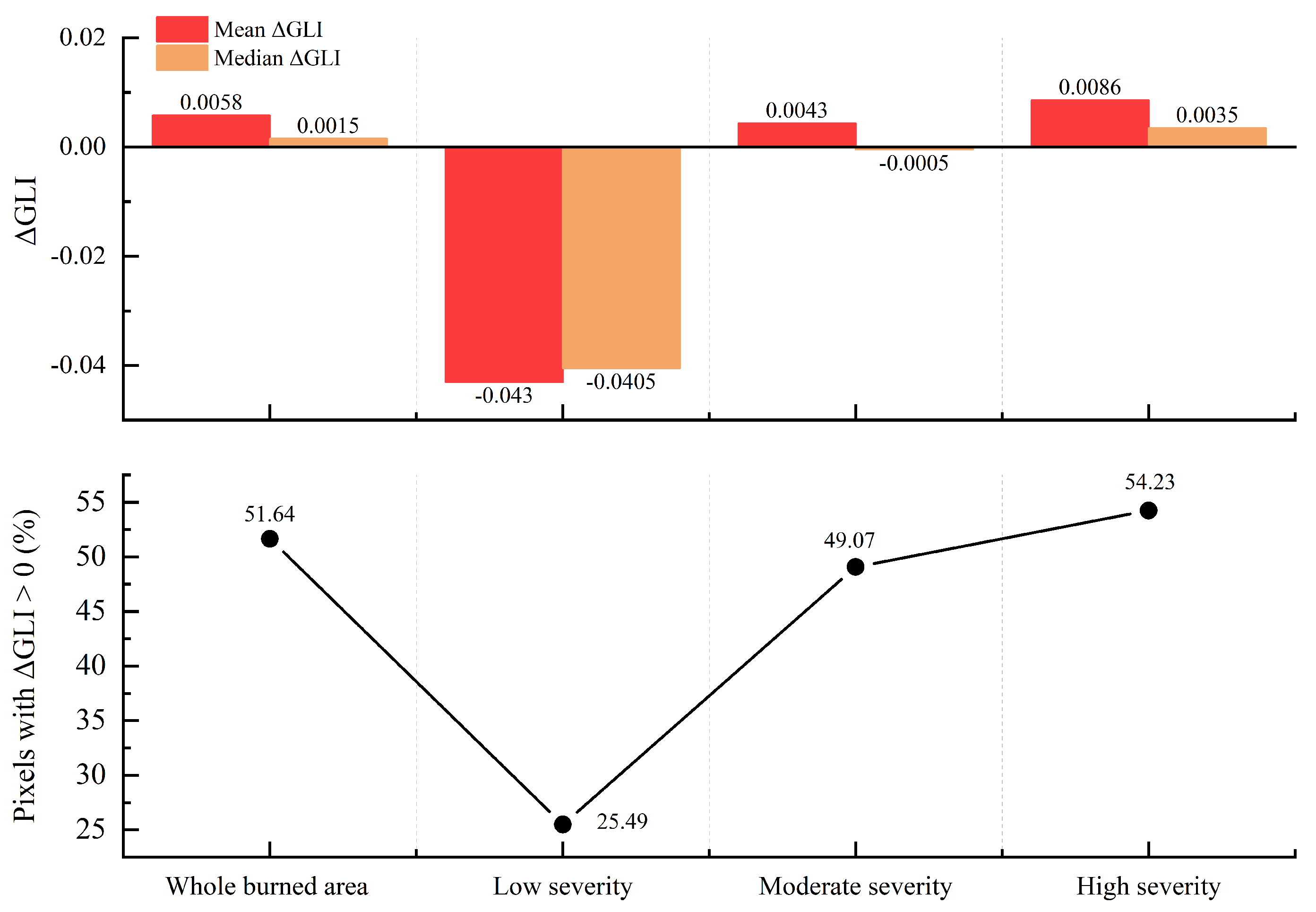
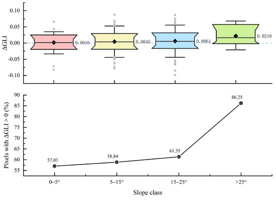
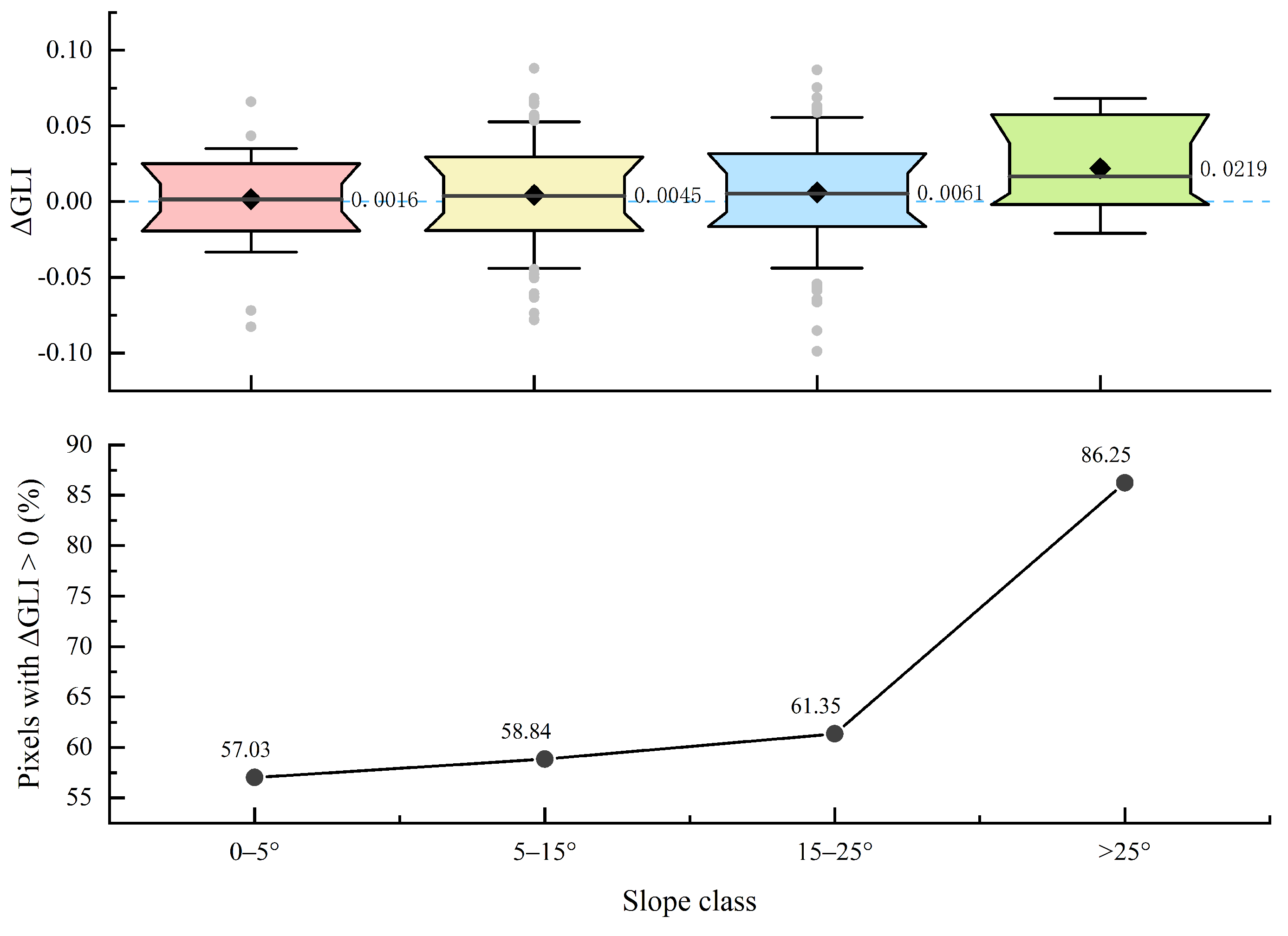
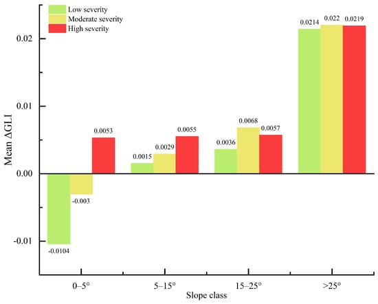
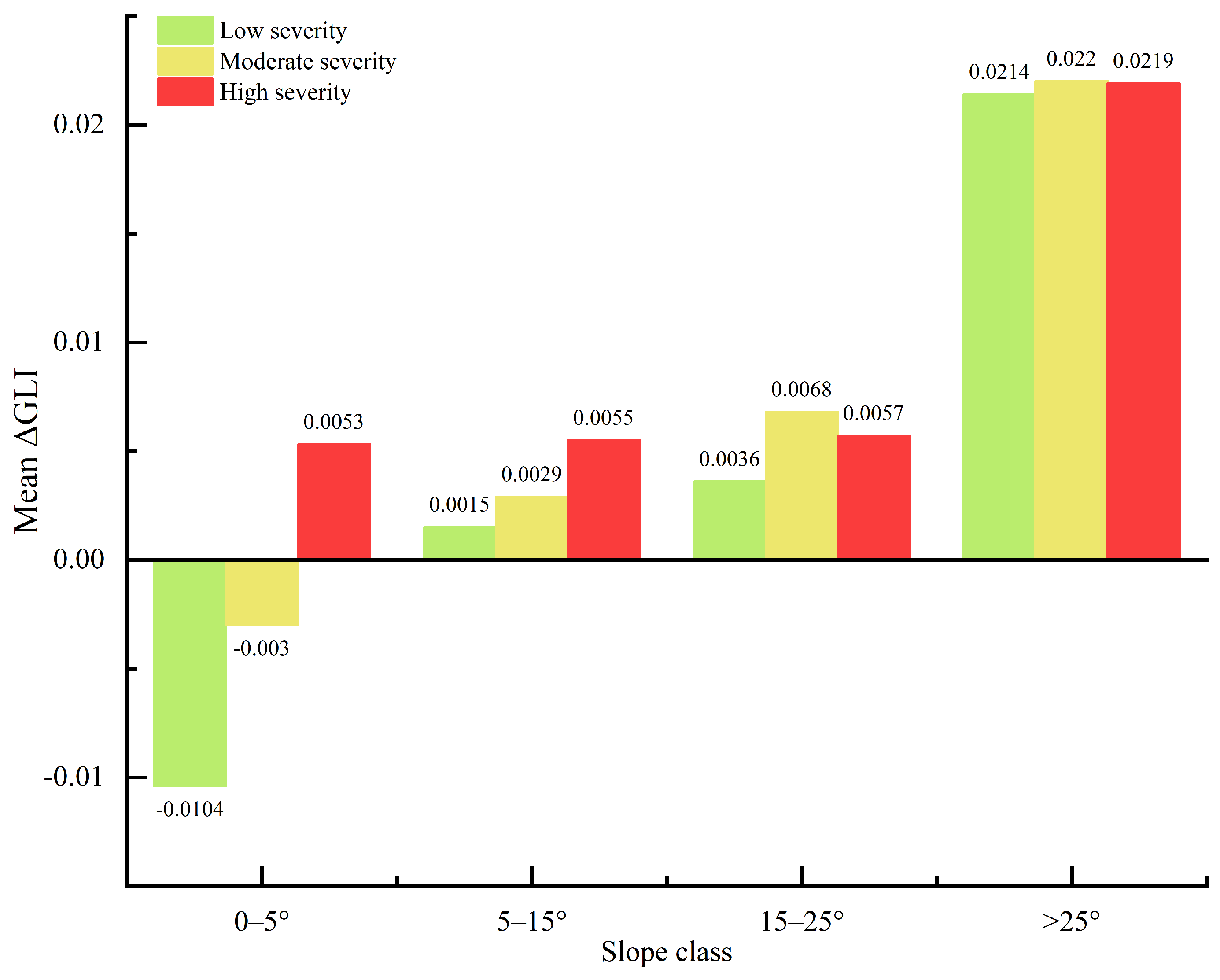
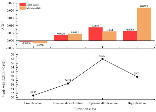
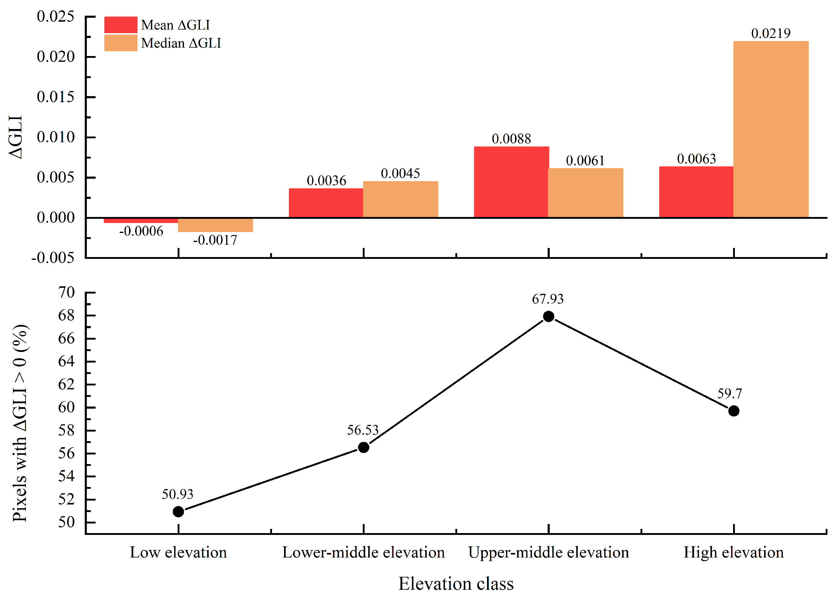
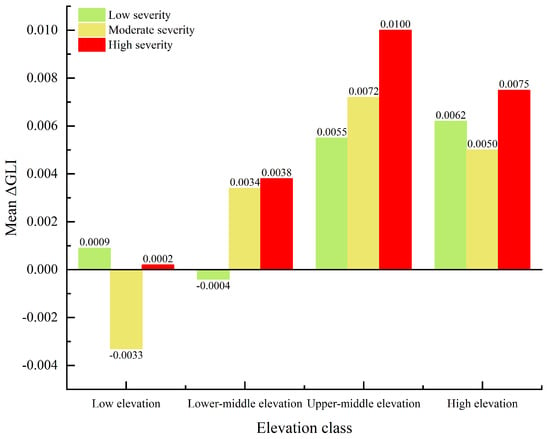
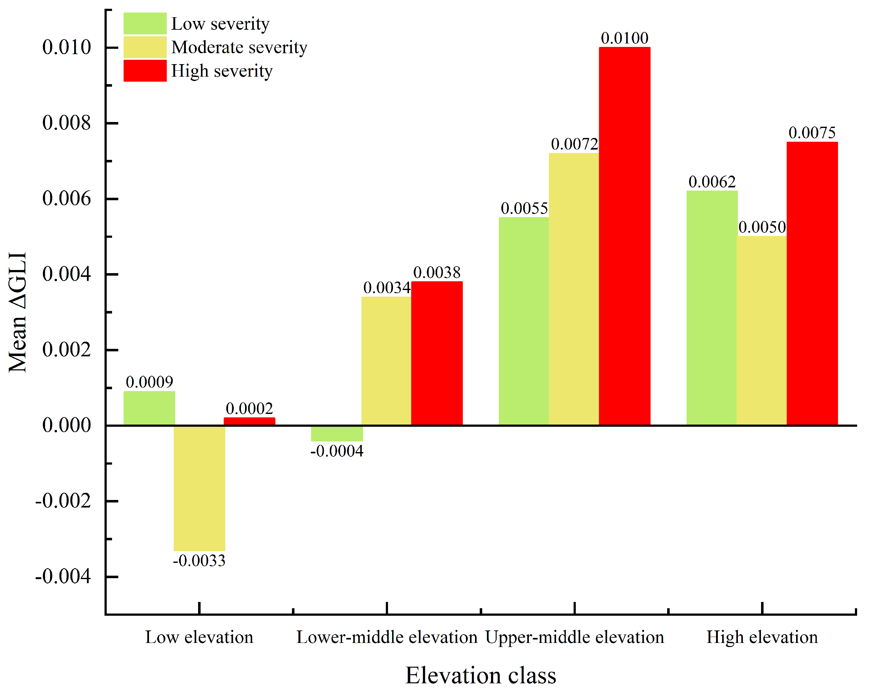
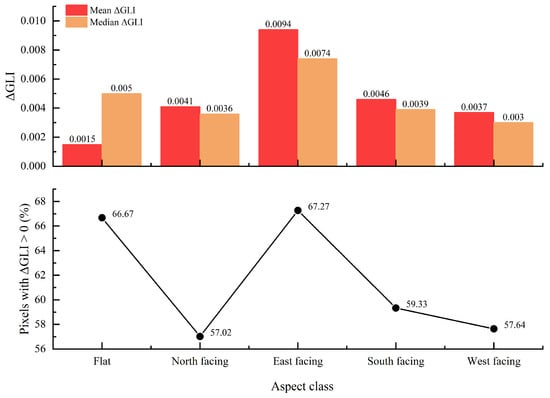
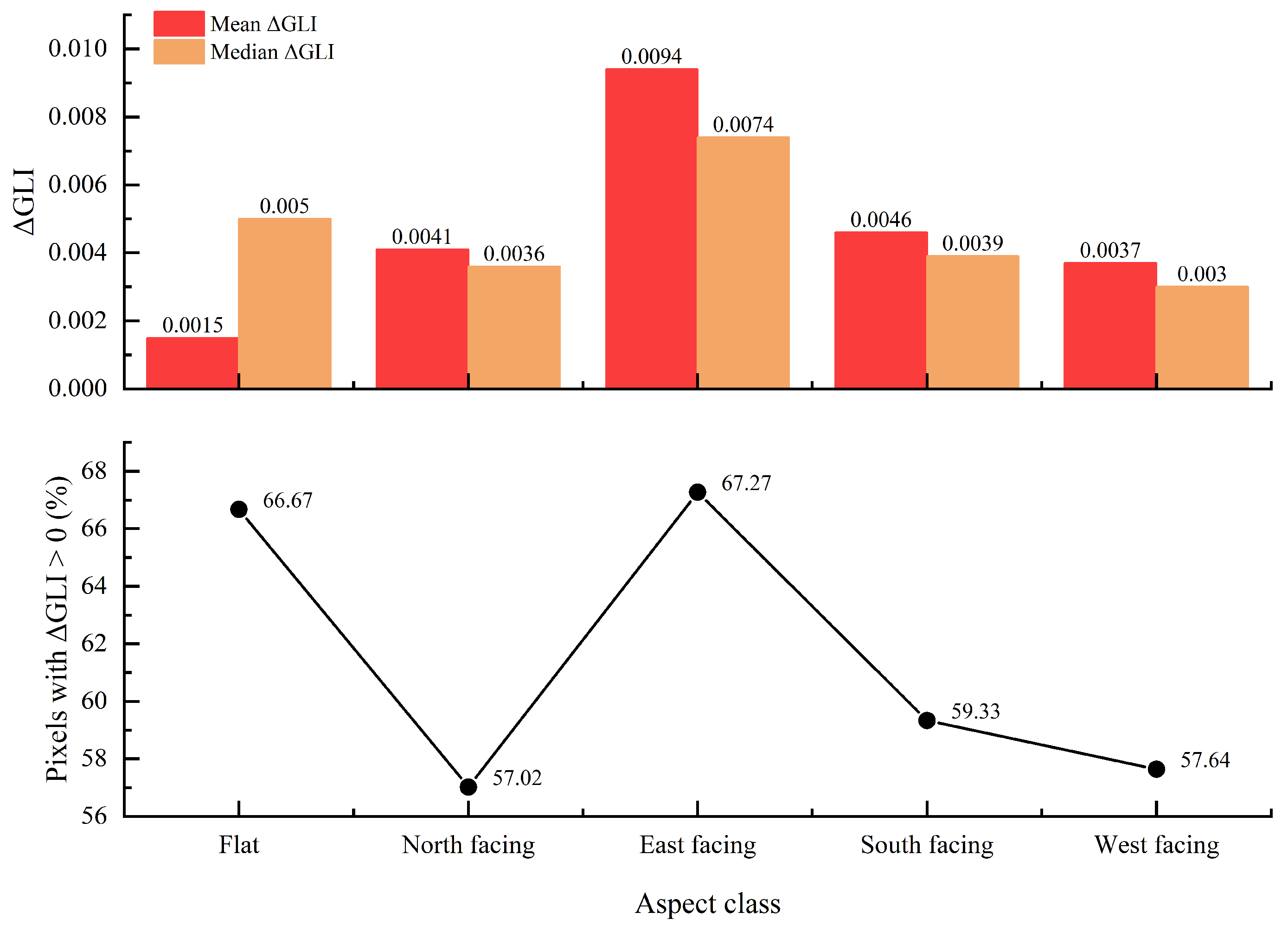
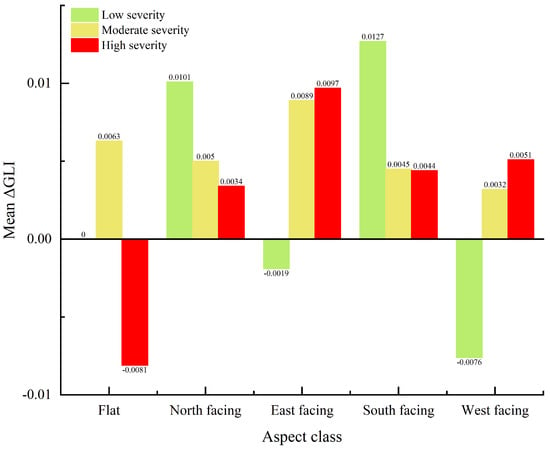
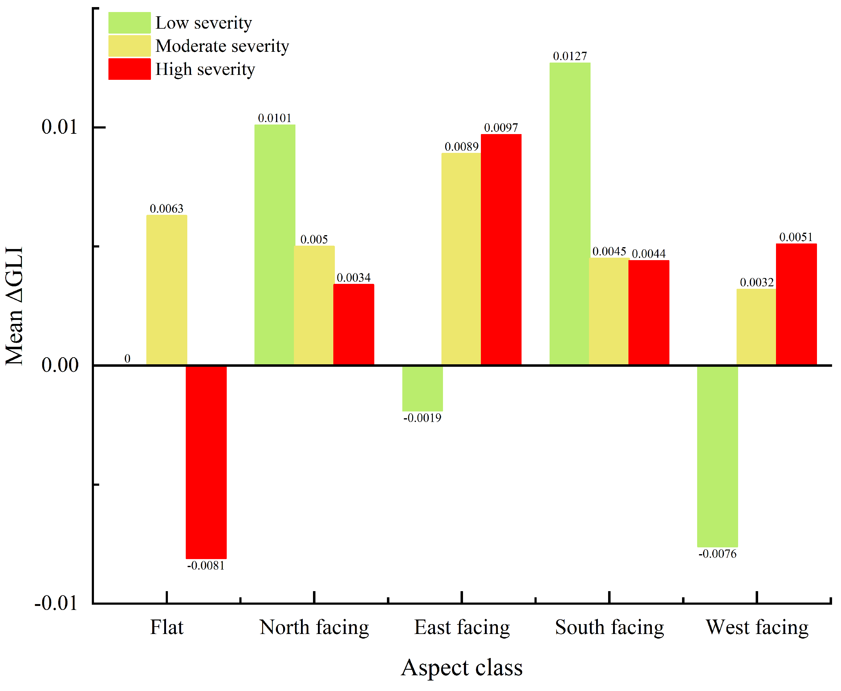

Disclaimer/Publisher’s Note: The statements, opinions and data contained in all publications are solely those of the individual author(s) and contributor(s) and not of MDPI and/or the editor(s). MDPI and/or the editor(s) disclaim responsibility for any injury to people or property resulting from any ideas, methods, instructions or products referred to in the content. |
© 2026 by the authors. Licensee MDPI, Basel, Switzerland. This article is an open access article distributed under the terms and conditions of the Creative Commons Attribution (CC BY) license.