


Highlights
What are the main findings?
- A deep feed-forward neural network (WNN) outperforms the classical Fire Weather Index, improving AUROC by 7–21% considering historical configurations.
- Integrating meteorological, FWI-derived, geomorphological, land-use, and anthropogenic variables captures fire susceptibility patterns that FWI alone misses.
What are the implications of the main findings?
- WNN is operationally deployed as P-FireCast within the PANORAMA platform, generating daily 4-day-lead susceptibility maps for a Mediterranean wildfire hotspot region.
- The approach enables more precise delineation of risk-prone areas, supporting targeted pre-positioning of firefighting resources in early-warning systems.
Abstract
Wildfires in the Mediterranean are expected to become increasingly frequent and intense under climate change and increasing drought conditions. Owing to the growing computational capabilities of modern GPUs, deep learning approaches are increasingly being adopted for wildfire modeling and often outperform conventional methods. This study presents a deep feed-forward neural network, named the Wildfire Neural Network (WNN), designed to generate daily wildfire susceptibility maps. The model integrates meteorological variables, FWI-derived indicators, geomorphological attributes, land-use information, and anthropogenic proxies. WNN was trained and validated using multi-year data from Calabria, southern Italy, a Mediterranean wildfire hotspot. Compared with the operational Fire Weather Index baseline, WNN achieved higher AUROC values and greater spatial information content, with AUROC improvements of approximately 7% to 21% considering the historical configurations.
1. Introduction
Wildfires affect ecological, hydrogeological, and public-health domains. Beyond the immediate loss of vegetation and wildlife, fires degrade soils and erode biodiversity [1]. Removing vegetation cover and sealing burnt soils reduce slope stability and amplify erosion, increasing hydrogeological risk [2]. Combustion also releases toxic substances that directly threaten human health [3,4]. A changing climate increases the probability of wildfires, where rising temperatures coincide with prolonged dry periods, such as in the Mediterranean region [5,6], because dry vegetation is prone to fueling wildfires and favoring their ignition and spread. Efficient risk management can mitigate the consequences of increased wildfire hazard. Recent fire seasons have been particularly severe across the European Mediterranean: 2017, 2022, and 2023 rank among the most extreme on record, and the fire season is lengthening, with serious wildfires occurring both earlier and later than the traditional summer window [7]. Projected exacerbation of summer weather conditions is expected to further increase extreme-fire potential in a warming climate [8], potentially rendering protection programs designed for ‘normal’ conditions ineffective. This threat is particularly severe for regions like Calabria, in the south of the Italian peninsula, which are especially exposed to frequent drought [9] and climate-change impacts [10], and where wildfire activity remains persistently high [11], contributing intensely to national emissions from forested land [12].
Improved wildfire risk management relies on accurate forecasts of the increased likelihood of wildfire occurrence and propagation. Since weather conditions play a significant role, fire weather indices (i.e., indices that rely solely on meteorological inputs) are commonly used. The most famous and operationally used is the Canadian Fire Weather Index FWI [13], which was selected in 2007 for fire danger assessment within the European Forest Fire Information System (EFFIS) network. FWI-based forecasting systems are currently in operational use, coupled with numerical weather prediction systems, at scales ranging from continental (e.g., for Europe, driven by ECMWF-IFS and Météo-France forecasts: https://forest-fire.emergency.copernicus.eu/apps/effis.csv; last access: 19 October 2026) to local (e.g., for Calabria: https://cesmma.unical.it/cwfv2/ or https://panorama.cesmma.unical.it/user-area/map variable name FWI; last access: 19 October 2026). Although fire weather indices effectively identify potentially dangerous meteorological conditions, they have inherent limitations for forecasting potentially fire-affected areas because they only partially account for predisposing factors and do not explicitly represent ignition triggers, particularly those related to human activities. Furthermore, regarding the former factors, not only land cover but also certain geomorphological features can be included as factors that enhance fire susceptibility. For example, in Calabria, from 2008 to 2019, 54% of wildfires occurred on slopes >35° and 31% on south-facing slopes [14]. Identifying and forecasting triggering factors is even more challenging because they primarily involve human behavior (the probability of fire ignition from natural causes, such as lightning, is very low) and cannot be addressed by traditional techniques based on physical equations that represent natural processes. Nevertheless, even in human behavior, some general rules can be detected [15,16]. For example, during the same period (2008–2019), 55% of ignition points were located within 100 m of a road. These habitual behaviors can be collected and used in forecasting systems that are not based on mechanistic processes but on evolutionary approaches, such as machine learning/deep learning methods.
Deep learning (DL) applications have expanded considerably over the last decade, owing to their success across several domains, increased computational power, and the growing availability of large datasets. This expansion extends to natural-hazard applications, including wildfire management, which is particularly complex because many factors affect it [17]. DL models have been applied to fire detection using ground-based visible cameras [18], smart CO2 sensors [19], and satellite images [20]; wildfire susceptibility mapping [21,22,23]; and wildfire spread prediction [24,25,26].
A growing body of work has explored the relationship between the FWI and data-driven models in three distinct ways. A first group of studies treats the FWI, or its sub-components (FFMC, DMC, DC, ISI, BUI), as input features within ML/DL models alongside vegetation, topographic, and anthropogenic drivers; in a Mediterranean-wide application covering southern Italy, Random Forest (RF) combined with explainable AI identified the FWI as the globally most influential predictor, while local attributions revealed the complementary role of NDVI, slope, and land cover [27]. Within the same modeling paradigm, Random Forest has also been used to derive national-scale wildfire susceptibility maps for Italy [28]. Still within this RF/SVM (Support Vector Machine) paradigm, Piralilou et al. [29] produced wildfire susceptibility maps for a Mediterranean forest region by fusing topographic, climatic, and anthropogenic conditioning factors derived from remote-sensing data of different spatial resolutions. A second group used the FWI as a benchmark to be outperformed: in the Eastern Mediterranean, Kondylatos et al. [30] showed that temporally-aware DL models exceeded the FWI in next-day fire-danger skill, with subsequent studies confirming DL superiority over the FWI. In the same region, Apostolakis et al. [31] proposed a complete machine-learning pipeline for operational next-day forest-fire risk estimation, in which the careful selection of non-fire (negative) samples was used to cope with the strong class imbalance between burned and unburned locations. A third group applied ML/DL to forecast or refine the FWI itself [32], including recent neural architectures benchmarked across Italy [33].
In this work, FWI and its sub-components are used both as meteorological predictors of the proposed model and as the baseline against which the model is evaluated, combining the first two approaches described above. By including FWI among the predictors, the herein presented model exploits the physically based meteorological information already synthesized by the index. At the same time, the comparison with FWI alone quantifies the added value of geomorphological, land-use, and anthropogenic predictors. Unlike several studies that employed reanalysis, global gridded, or low-resolution datasets, our models were trained and validated using high-resolution data (17 out of the 21 predictor variables in the original dataset, alongside the on-field detected burned areas) whose accuracy had been specifically assessed by [11], allowing for a more reliable evaluation of the network’s added value beyond the classical FWI calculation.
This paper assesses the effectiveness of a DL-based approach for forecasting wildfire-exposed areas compared with the classical physically based FWI method used operationally in the Calabria Region. We used a deep feed-forward neural network (DFFNN). For conciseness, the developed model is hereafter referred to as the Wildfire Neural Network (WNN). The WNN was applied across the entire Calabria region (Italy) to produce daily wildfire susceptibility maps using high-resolution, spatially distributed observed meteorological variables. The network was trained and validated over 9 years of data [11]. A tuple of up to 18 input variables, subdivided into time-variant meteorological data and time-invariant geomorphological and land use data, was considered for each 100 × 100 m grid cell in which the study area was subdivided. Factors related to human behavior were also considered during the training phase, such as distance to roads and urban centers. Moreover, two different data sampling techniques were investigated.
Specifically, in this study, wildfire susceptibility is defined as the probability that a 100 m × 100 m grid cell is affected by a wildfire event under given meteorological, geomorphological, land-use, and anthropogenic conditions. It should not be interpreted as wildfire risk in the strict sense, since exposure and vulnerability are not explicitly modeled. Furthermore, with respect to [11], this paper focused on the operational applicability of the WNN and on its added value with respect to the FWI currently used in operational practice.
The specific goals are: (i) to describe the WNN architecture and provide details about its training, including information about the dataset and the sampling procedures applied; (ii) to compare the WNN performance in terms of accuracy and information content to FWI; and (iii) to assess possible advantages of the DL-based approach in operational use contexts.
The paper is organized as follows. Section 2 describes the study area and the WNN model. It details the inputs and outputs, data sampling techniques, training, validation, and test periods, and the system architecture. Section 3 presents the results and compares them with those obtained using FWI. Finally, Section 4 discusses and summarises the main findings and outlines future perspectives.
2. Data and Methods
This section first describes the study area, then presents the proposed WNN model and details its application, and finally outlines the system’s overall software architecture.
2.1. Study Area and Period of Analysis
The Calabria region (southern Italy) is a peninsula of approximately 15,000 km2, extending mainly north–south, with a coastline of about 800 km. The region is characterized by a complex, steep orography, with only 9% of the area covered by flat terrain. Its geographical location and geomorphology produce a non-uniform precipitation distribution, with annual precipitation ranging from 600 to 1500 mm [34]. The summer period is generally dry due to high temperatures, which lead to more frequent wildfires [35].
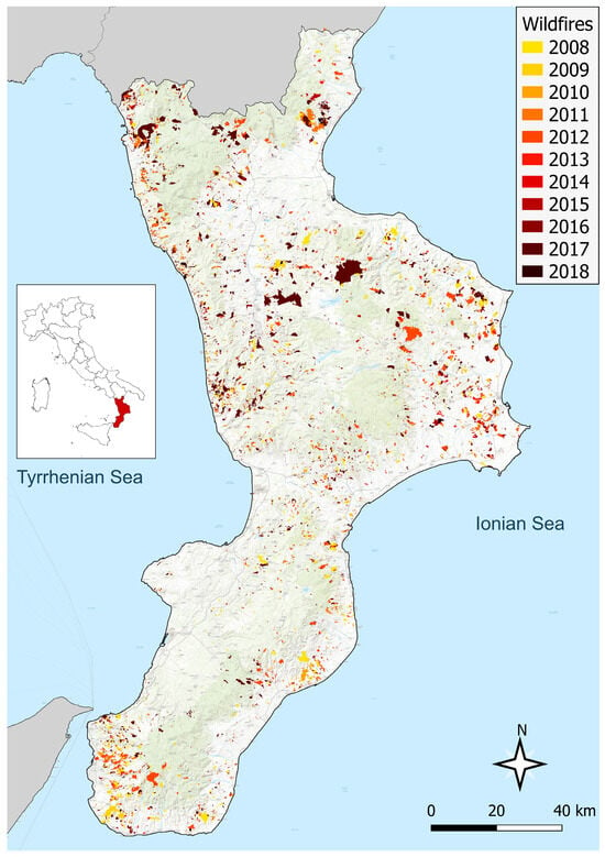
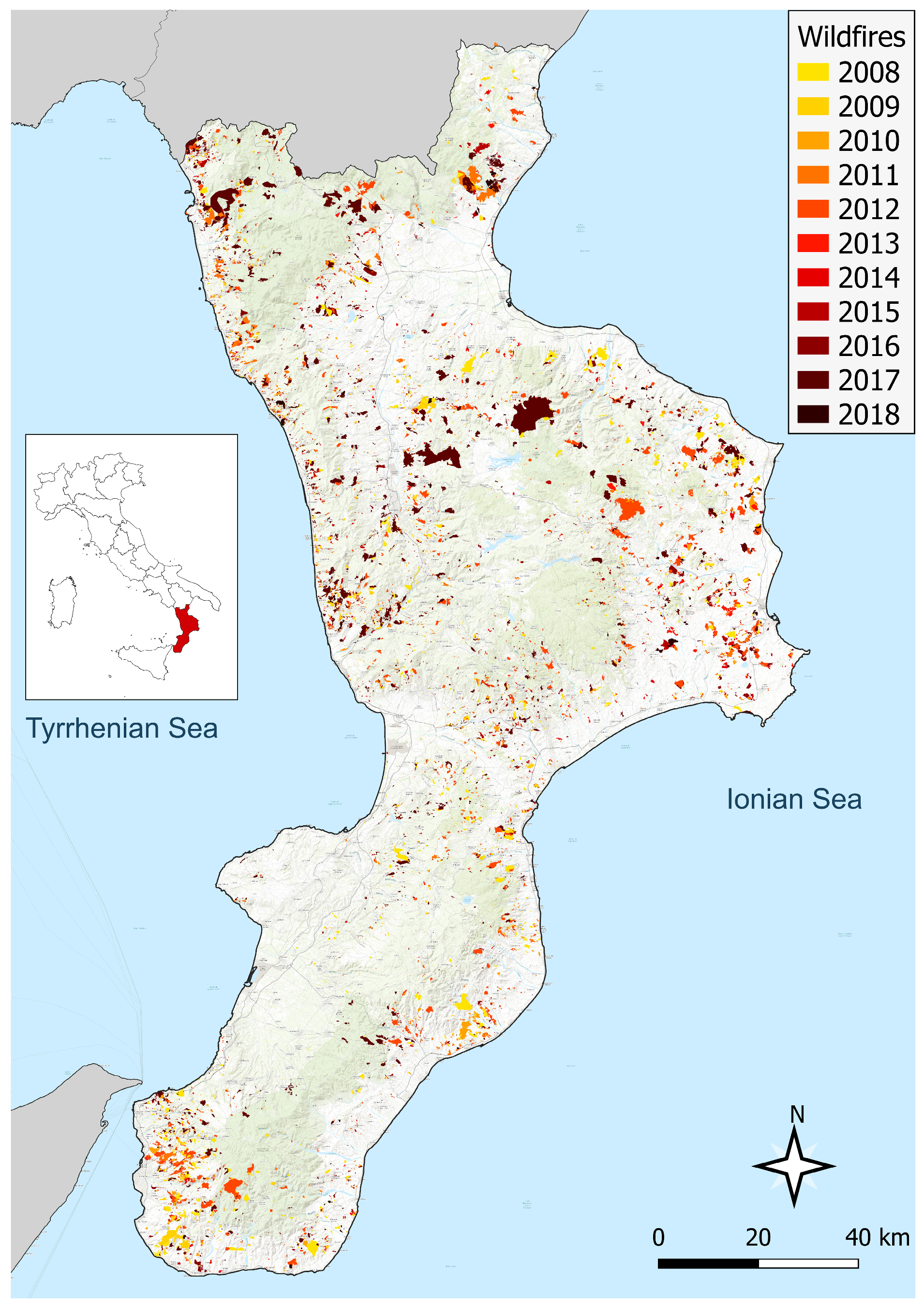
The peninsula is covered by approximately 40.6% forest (612,932 Ha), making it among Italy’s greenest regions and home to three National Parks and one Regional Park. The characterization of forest types is highly heterogeneous [36]. This work uses the land cover classification proposed by the Calabria Region at a spatial resolution of 100 × 100 m, which follows the same strategy adopted in the Corine Land Cover Project (CLC [37]). In particular, the “CUT—Carta Usi del Territorio” 2020 [38] expands the CLC details by introducing levels IV and V. A wildfire susceptibility index was assigned to each land cover class, ranging from 0 (urban areas) to 100 (cork woods), following the Italian Manual for determining the Wildfire Risk Plan in National Parks [39,40]. From 2008 to 2018, the responsible authority, “Comando Unità Forestali, Ambientali e Agroalimentari dei Carabinieri”, detected 9076 fires (Figure 1), corresponding to 120,431 Ha [14]. All wildfire data were collected through field surveys, and each event is dated by its detection date regardless of duration. This choice reflects the reporting authority’s protocol: only report dates were recorded in 2008–2015, and intervention and suppression dates were introduced later and not compiled systematically, so the detection date was used as the sole reference across the dataset. Between 2008 and 2018, the region reported 9076 wildfires. Following [11], we restricted the analysis to wildfires that occurred during the April–October fire season, which accounted for 8609 fires (95% of the total) and 116,880 ha of burned area (97.1% of the total). The most affected year was 2017 [12], with approximately 32,055 ha burned, corresponding to approximately 1500 ignitions.
Figure 1.
Wildfire burnt areas between 2008 and 2018. Each color refers to a specific year. The total burnt area is approximately 120,430 Ha, with over 9000 ignitions (source: [11], based on data from the Comando Unità Forestali, Ambientali e Agroalimentari dei Carabinieri, the Carabinieri Command of Forestry, Environmental and Agri-food Units, the official body responsible for surveying burned areas).
For this work, the study area was discretized into 100 m × 100 m grid cells, yielding 1,403,027 land cells potentially exposed to fire events. Most of the dataset was derived from [11], whose analysis adopted the TILE-strategy approach; in contrast, the present study focused primarily on the local, single 100 m × 100 m grid cell observed on a specific day of the fire season.
Meteorological variables were derived through spatial interpolation of station measurements from the Regional Monitoring Network, with all meteorological inputs, intermediate FWI components, and the final FWI computed on a common 100 m grid. Based on data availability, the study spanned 11 fire seasons from 2008 to 2018, each defined as running from April 1 to October 31. The monitoring network (159 rain gauges, 104 temperature stations, 30 humidity stations, and 29 wind stations) provided data that we first validated by removing unrealistic values and reconstructing the resulting gaps (under 0.5% of total records) through correlation with the nearest station. Each variable was subsequently interpolated onto the 100 m grid using an approach tailored to its behavior: precipitation, aggregated as 24-h cumulative totals, was interpolated via Inverse Distance Weighting, which also enabled derivation of the number of consecutive dry days; air temperature was interpolated using cubic splines combined with elevation-based regression (R2 = 0.84); relative humidity followed a comparable approach incorporating temperature as an additional predictor (R2 = 0.91); and wind speed was interpolated using cubic splines. Further methodological details are provided in [11].
2.2. WNN Model Details
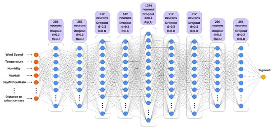
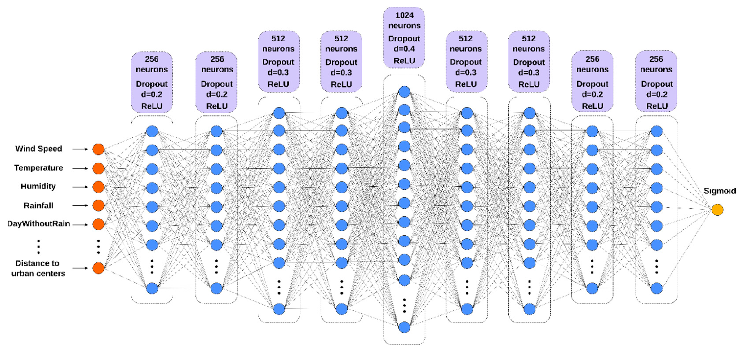
The WNN model is a feed-forward deep neural network designed to estimate the daily likelihood that a 100 m × 100 m grid cell is affected by a wildfire event. The model predicts the probability that a grid cell is affected by wildfire based on input features that characterize the site. The network input is a tuple of up to 18 site state variables, listed in Table 1, which we assumed were relevant for fire prediction in the study area. The tuple size depends on the training set type, as described in Section 2.2.2 below. The WNN output, i.e., the site’s probability of being affected by fire, can be further processed by applying a threshold to obtain a binary classifier. We will refer to Foff and Fon as the binary outcomes representing negative (less than or equal to the threshold) and positive (greater than the threshold) predicted fire conditions, respectively. Figure 2 shows the WNN with all 18 variables in Table 1 used as inputs. We selected the final architecture based on preliminary sensitivity experiments to balance predictive performance, computational cost, and overfitting control.
Table 1.
Daily (2008–2018) and time-invariant input features for the WNN.
Figure 2.
Graphical representation of the WNN model. The number of neurons, the dropout percentage, and the ReLU activation function are shown in the violet boxes. Inputs and output are identified by orange and yellow circles, respectively, while blue circles indicate the neurons of each layer.
With a reduced tuple size, the network loses a few input neurons corresponding to the missing input variables, while the hidden and output layers remain unchanged. To obtain a spatially extended forecast map, we partitioned the study area into cells and applied the network once per cell. This study used a regular square cell grid, although other structured and unstructured grids could be considered.
The network was trained by minimizing the binary cross-entropy loss function L:
where N is the number of training samples, yi is the observed binary label of sample i, with yi = 1 for fire and yi = 0 for no-fire conditions, and p(yi) is the probability predicted by the WNN.
To minimize the loss function, we applied the Adaptive Moment Estimation (Adam) gradient descent algorithm [41]. Moreover, except for the output layer, where the sigmoid function is applied, the rectified linear unit (ReLU) was used to address the vanishing gradient problem, which makes it hard to determine the appropriate direction for improving the cost function [42].
To prevent overfitting, a common phenomenon in which a neural network performs too well on the training set but not on other datasets, we also considered L2 regularisation and dropout techniques [43]. Table 2 summarises the WNN parameters adopted in this work, which we empirically set through preliminary tests conducted on the study area.
Table 2.
WNN hyperparameters.
2.2.1. Daily and Time-Invariant Inputs
The 18 variables listed in Table 1, which serve as inputs to the network, are divided into daily and time-invariant inputs; the latter vary only across space (i.e., with the cell’s coordinates).
Daily inputs are climatic observed data (wind speed, temperature, relative humidity, rainfall) and FWI components (DC, DMC, FFMC, ISI, BUI, FWI), which were calculated using the cffdrs R package (Canadian Forest Fire Danger Rating System, version 1.8.2047, available at https://www.rdocumentation.org/packages/cffdrs/versions/1.8.20, accessed on: 29 October 2026). In addition, we derived two other daily variables: tdry, representing the number of days without rain, and tlf, the time since last fire, defined as the number of days elapsed since the most recent fire in the cell. This index captures information on past fires and potential fire recurrence in the cell. In this study, it was capped at approximately two years (731 days), beyond which a previous fire is assumed to have no further influence on the cell.
CUT, DTM, aspect, and slope are time-invariant inputs. We also computed two additional time-invariant inputs: dr, the Euclidean distance to the nearest road, and du, the Euclidean distance to the nearest urban center. Since 55% of fires occurred within 100 m of a road during the analysis period, these variables were hypothesized to be relevant to the inclusion of human factors in wildfire susceptibility prediction.
Compared with the aforementioned work [11], we employed four groups of predictors at the original 100 m × 100 m resolution, without the tiling strategy: Climatic variables (temperature, wind speed, precipitation and relative humidity); the FWI and its Intermediate Index (FFMC, DMC, DC, ISI and BUI); Morphological and Land Cover variables (DTM, aspect, slope and land-use index); and Human Factors (distance to roads and to urban centers). In addition, we included the tlf index, computed as described above.
2.2.2. Training Set Types
Based on the above-described input variables, three training set types (i.e., combinations of input variables) were considered, as shown in Table 3. As the name suggests, the ALL set includes all 18 variables listed in Table 1. The FWI-based set comprises 8 variables: seven shared predictors (DTM, Land use, Slope, Aspect, Distance to roads, Distance to urban centers, and tlf) plus the FWI. The CLIMATIC-based set uses the same seven shared predictors but replaces the FWI with the basic climatic variables (Wind Speed, Temperature, Relative Humidity, Rainfall, and DayWithoutRain), for a total of 12 variables. Note that all training set types account for human factors. Moreover, the redundancy in the ALL-training set type allowed the neural network to perform implicit feature selection during training. Comparing the ALL, FWI-based, and CLIMATIC-based configurations also serves as a partial removal experiment, providing insight into the relative contribution and added value of the different predictor groups.
Table 3.
The three training set types used to train the WNN.
2.2.3. Data Sampling Options
Depending on the extent of the study area, the input data can be extremely large. Because the dataset combines more than 1.4 million grid cells with daily observations over several fire seasons, the resulting number of potential cell-day samples is extremely large. Therefore, sampling strategies were required both to reduce the computational burden and to address the strong class imbalance between the fire and no-fire samples (e.g., [44]).
By considering that approximately 95% of cells of the study area were never affected by fire and 5% were affected by a fire at least once in the whole period of analysis, we tested two sampling strategies, namely random and historical, to balance the sets of cells provided to the network so that the number of cells in the state Foff was similar to that in the state Fon. For a given training-period day, random sampling selects all fire-affected cells and Nnf randomly selects non-ignited cells. Nnf was empirically set to 2700 based on preliminary experiments conducted in the study area. The historical sampling considers the entire fire history of the study area. Given a day in the training period, a historical fire map is calculated as follows: a cell is labeled True if at least one fire occurred in the corresponding area during the interval from the beginning of the training period to the current day, and False otherwise. Therefore, the historical sampling dataset was created by selecting:
- All the cells affected by fire on the current day;
- A total of Nnf/2 randomly selected cells not affected by fire on the current day but affected by at least one fire in the past period of analysis;
- A total of Nnf/2 randomly selected cells are never affected by fire.
In addition, the weight balancing (WB) strategy was adopted, which updates the training sample weights when computing the loss according to the following formula:
where n0 and n1 are the number of cells never ignited and ignited at least once over the study period in the training set, respectively, and size is the sum of n0 + n1.
wi = 0.5 ⋅ size/ni (i = 0,1)
2.2.4. Training, Validation and Test Periods
In this work, the analysis was extended to two training periods, with the datasets split strictly by time. The first, TP1 (Training Period 1), covers seven fire seasons (2010–2016) and is tested on 2017 and 2018. The second, TP2 (Training Period 2), adds the 2017 season to the training data (2010–2017) and is tested on 2018 alone. In both cases, we used no day from a test year during training. We excluded 2008 and 2009 from training because we could not compute the Last Fire Index for them, since its calculation requires the two preceding years of fire data. Within each training period, we randomly divided the sampled cell-days into a training set (80%) and a validation set (20%), using a class-stratified split so that both sets preserve the same proportion of burned and unburned samples. The two configurations also differ in the composition of their test periods. The TP1 test set spans two fire seasons, including 2017, a particularly severe season with 3206 burned cells, more than ten times the 2018 total (269 cells).
2.3. System Architecture
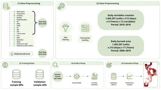
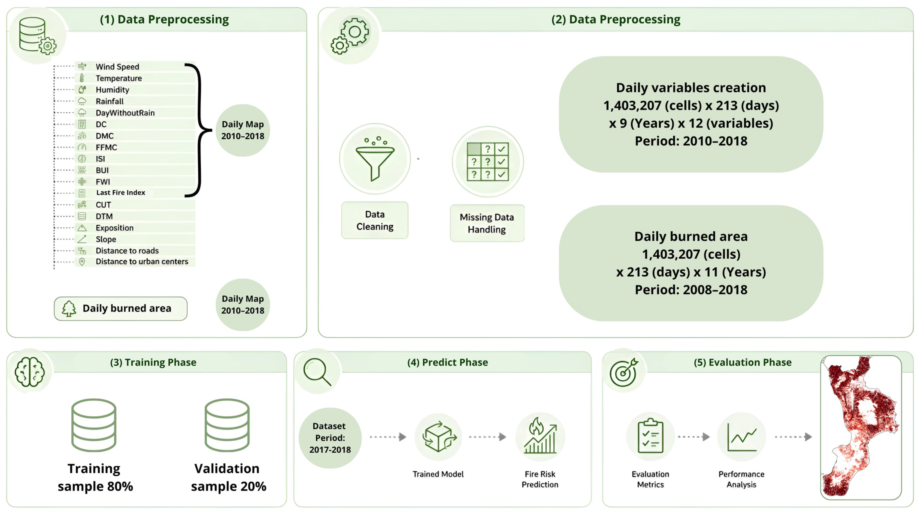
In addition to the WNN model, the application developed in this work is built on other fundamental components, each corresponding to a phase of the system’s execution. Figure 3 shows the system software architecture. The first phase focuses on data preparation, during which the required meteorological and geomorphological data are collected. The preprocessing data phase derives auxiliary inputs (such as human factors) and defines the overall dataset. The training phase splits the data into training and validation sets and trains the WNN. The trained network is ultimately used to generate wildfire susceptibility maps for the entire study area. For assessing susceptibility maps, the system uses threshold-based classification diagnostics and ROC analysis, including the area under the ROC curve (AUROC), complemented by precision-recall (PR) analysis and the corresponding area under the PR curve (PR-AUC). The PR-AUC was computed using bootstrapping with 10 resamples to estimate its uncertainty. Furthermore, the Shannon Entropy [45] was evaluated at the daily scale using the following formulation:
where p(xi) is the probability mass function of the values taken by the output map, i.e., the empirical probability of class i. Shannon entropy was computed on a daily basis using base-2 logarithms, and is therefore expressed in bits. For each model, the empirical probability distribution of the daily map values was estimated by grouping the grid-cell values into N = 25,000 equal-width bins over the interval [0, 1]. Since the WNN output already lies in [0, 1], no rescaling was applied to it, whereas FWI values were rescaled to [0, 1] using fixed bounds, with an upper threshold of 70, corresponding to the maximum value of the EFFIS fire danger classification. This analysis aimed to assess the information content of the maps produced by the employed models.
Figure 3.
Architecture and workflow of the developed application.
3. Experiments and Results
By considering the three training set types (Section 2.2.2), the two sampling options (Section 2.2.3), and the two training periods (Section 2.2.4) studied in this work, a total of 12 WNN learning experiments were performed to define 12 DL-based alternative trained networks for wildfire susceptibility prediction. Since the network was developed in Keras, which leverages CUDA 11.8 acceleration via the TensorFlow engine v1.13.1, the learning experiments were executed on a scientific workstation equipped with two Nvidia Titan Xp GPUs, each with 12 GB of dedicated memory. The Calabria region study area required about one week of compute time. Without GPU acceleration, the execution time would have been considerably higher, underscoring the crucial role of GPGPUs, and more broadly, of High-Performance Computing in DL applications. During the training phase, the input to the WNN model was fed in batches of 512 cells, each cell representing a tuple of up to 18 variables (depending on the training set type). At the end of each batch, the learning algorithm was applied. Training was performed for a maximum of 300 epochs, with an early-stopping criterion based on the validation loss: training was terminated when the validation loss failed to decrease by more than 10−4 for 30 consecutive epochs. The 12 trained networks were therefore applied to compile a wildfire susceptibility map for each day of the test period. For each day, one additional susceptibility map was compiled using the FWI method for comparison, for a total of 13 alternative susceptibility maps produced per day. All maps compiled using FWI and WNN had the same spatial resolution, matching the grid used to discretize the study area (100 × 100 m cells). This ensured consistency and enabled a more accurate comparison of the methods’ predictive capabilities.
3.1. AUROC and PR-AUC Assessment
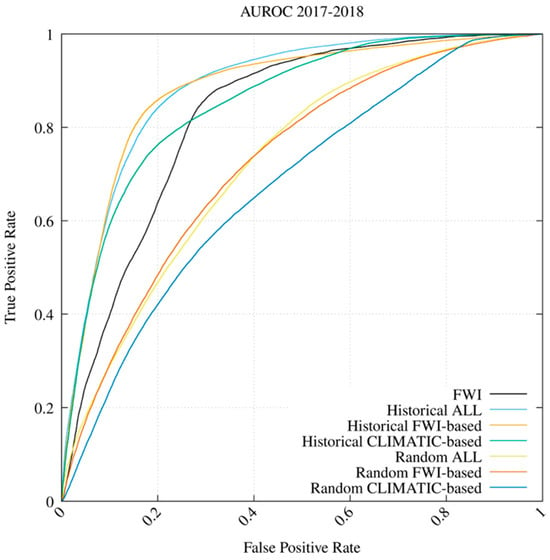
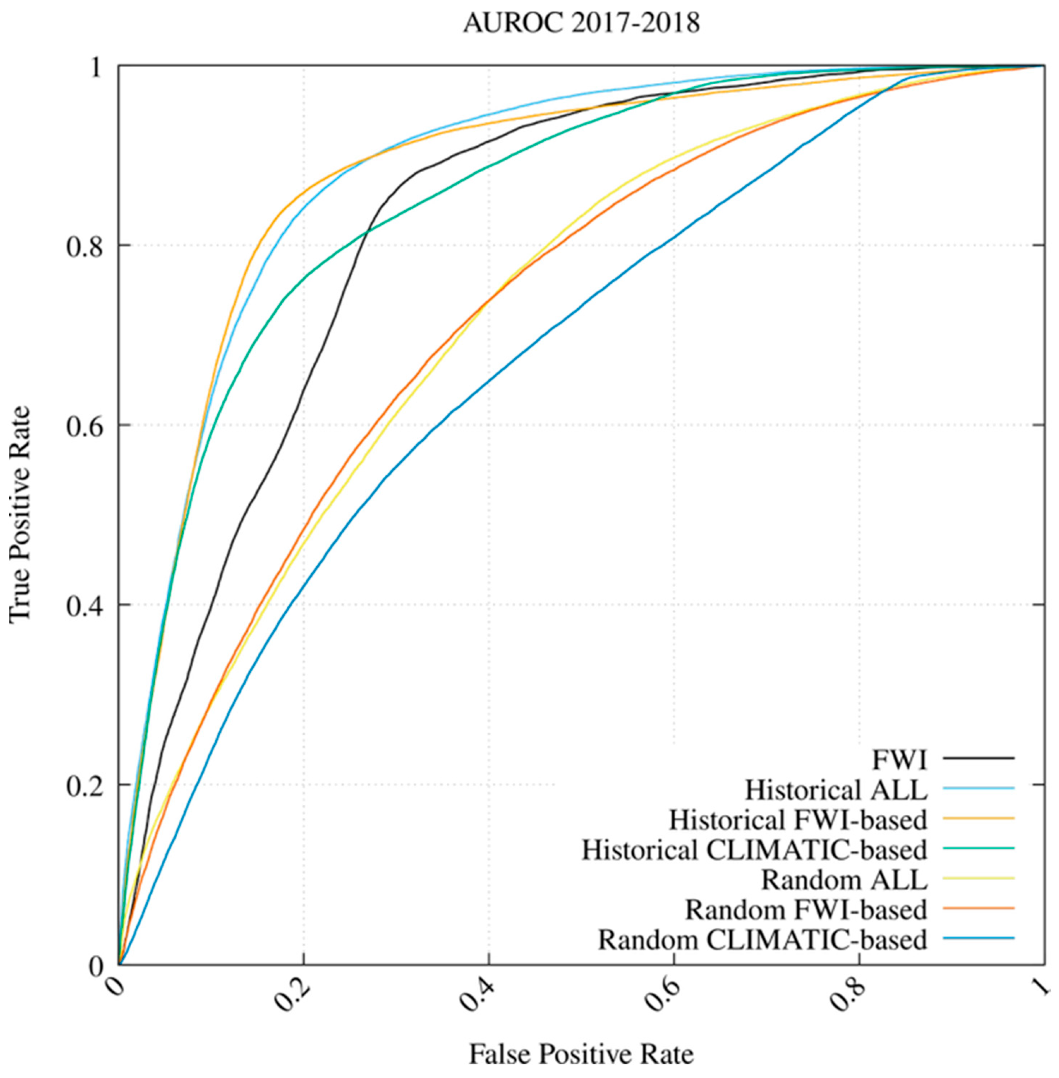
A comparative assessment of the first six trained networks with the reference FWI method over the TP1 period to predict the events that occurred from 2017 to 2018 is shown in Figure 4. As in [30], we collected an equal number of negative samples, i.e., non-ignited cells, as the number of fire events and assessed the efficacy using Receiver Operating Characteristic (ROC) curves and the Area Under the ROC Curve (AUROC). This process was repeated 10 times, and the mean and standard deviation of AUROC were computed and reported in Table 4. The results indicate that the WNN configuration combining FWI-related meteorological information with geomorphological, land-use, anthropogenic, and historical fire information outperformed the FWI-only operational baseline. In particular, the Historical CLIMATIC-based experiments, which do not use any information from the FWI system or its sub-components and are therefore independent of it, outperformed FWI. However, this improvement should be interpreted as the combined effect of the additional predictors and the WNN model, since the contribution of the network architecture alone was not isolated. Moreover, the advantage over FWI depends on the sampling strategy: all models trained with Random sampling performed below FWI in both testing periods.
Figure 4.
WNN vs. FWI comparative results in terms of AUROC for the 2017 and 2018 fire seasons (training period April 2010 to October 2016).
Table 4.
AUROC for all models considered. Left columns refer to the TP1 testing period (2017–2018), right columns to the TP2 testing period (2018). For each period, the first column reports the mean and the second the standard deviation.
The historical-ALL WNN yielded the best result, with an average AUROC of 0.884. Compared with the FWI performance of 0.824, WNN performed 7.3% better (i.e., (AUROCWNN − AUROCFWI)/AUROCFWI × 100). Moreover, the historical CLIMATIC-based WNN outperformed the FWI by 3.5%.
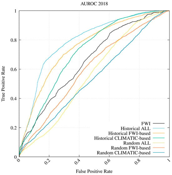
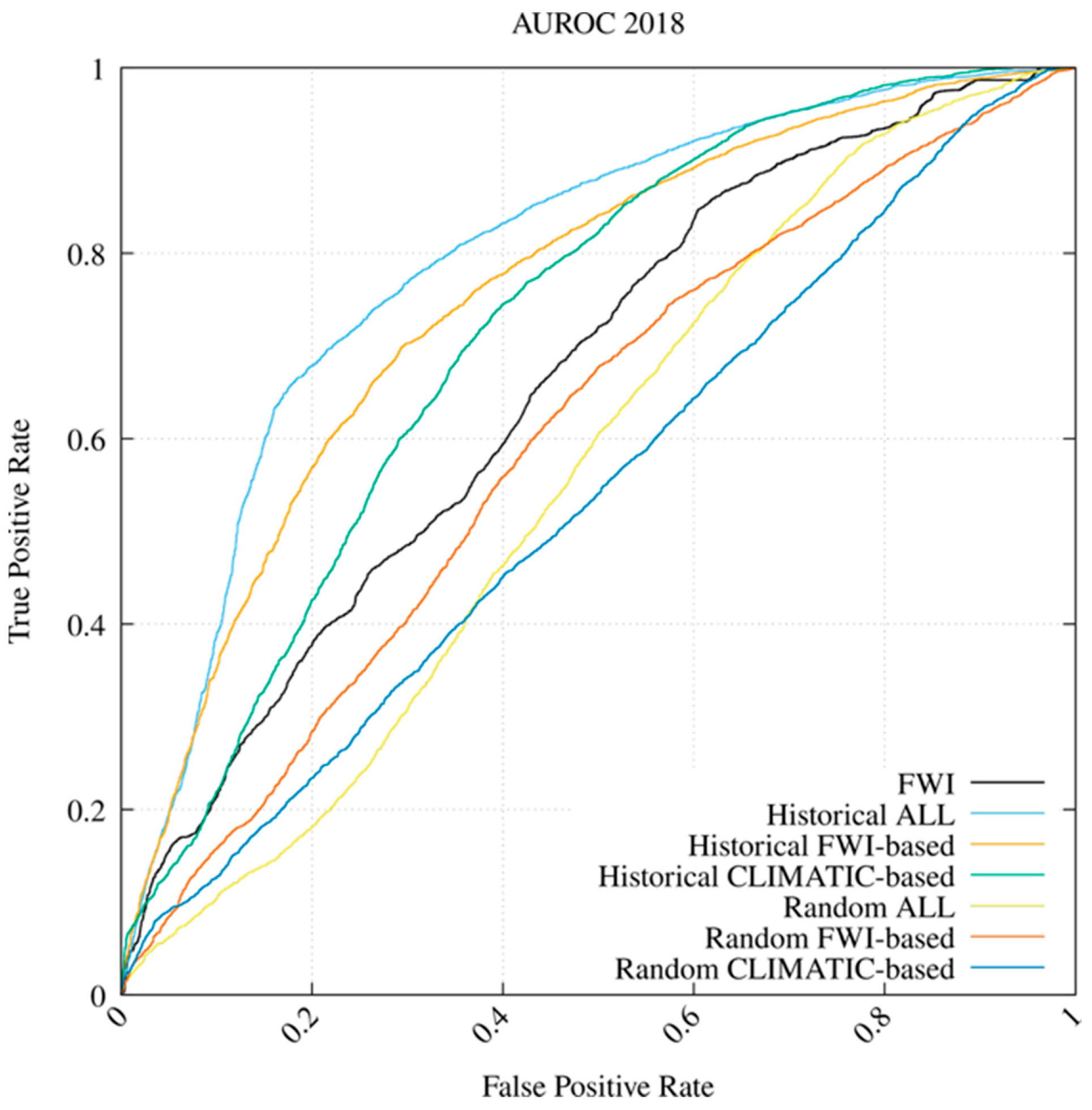
Figure 5 and Table 4 show the results for the remaining six trained networks over the TP2 period to predict events in 2018. The results further demonstrate that historical-based WNN models outperformed FWI in terms of AUROC, while the performance of the random-based models remained unsatisfactory. Here, the best result was still found in correspondence with the historical-ALL WNN, with an AUROC value of 0.796. Compared with the FWI performance of 0.661, WNN performed 21% better. Here too, the historical CLIMATIC-based WNN outperformed the FWI baseline by 14.4%.
Figure 5.
WNN vs. FWI comparative results in terms of AUROC for the 2018 fire season (training period April 2010 to October 2017).
In the analyzed cases, including temporal information, human-related data and other factors improved the WNN’s forecast of wildfire occurrence susceptibility. Overall, the historical ALL WNN achieved the highest AUROC. For this reason, it was assumed to be the reference WNN-based model for subsequent Map-based Visual, Shannon Entropy, and Quantitative Assessment.
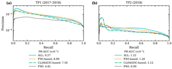
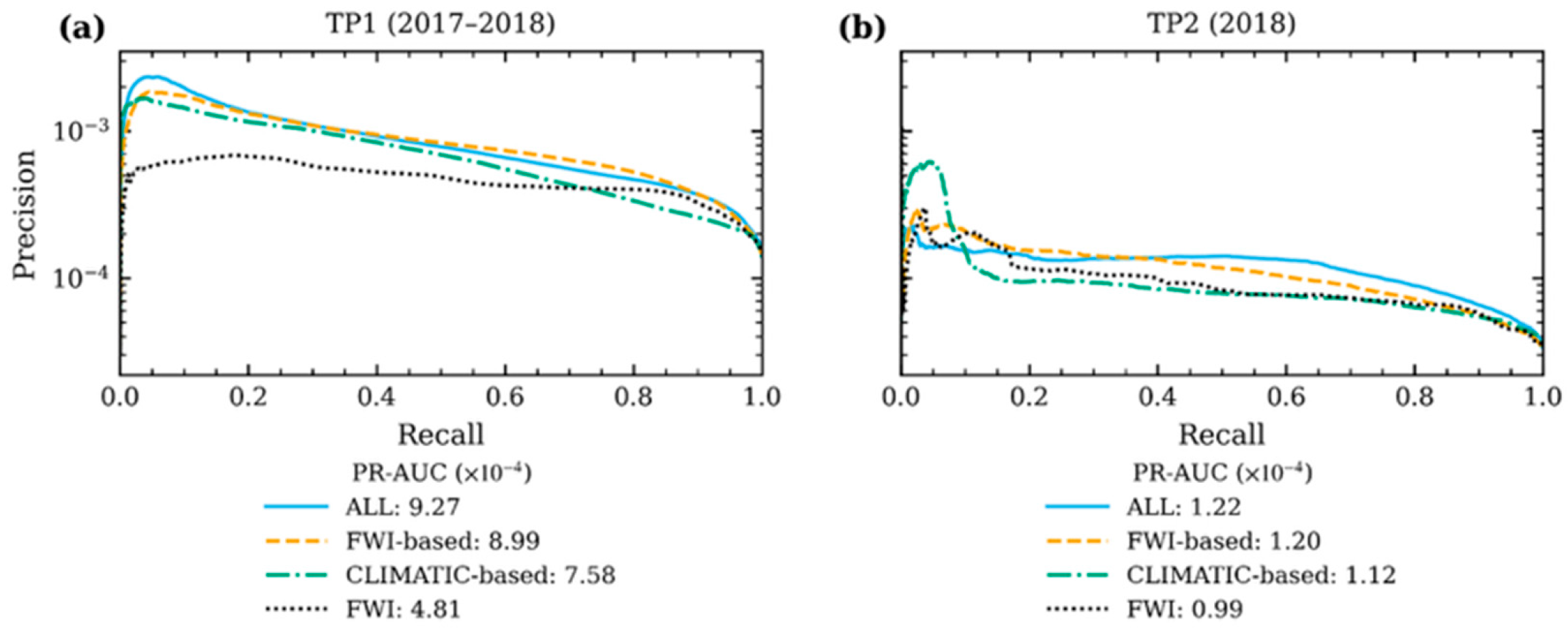
As a complementary analysis, Figure 6 shows the precision–recall (PR) curves for the three Historical configurations and the FWI for the two testing periods, TP1 (Figure 6a) and TP2 (Figure 6b); the legend values are the corresponding areas under the PR curve (PR-AUC). Precision is plotted on a log10 scale because of the strong class imbalance: the number of observed fire events (positive cases) is extremely small compared with the total number of cells potentially affected by wildfire. In this case, the WNN outperformed the FWI, as shown by the PR-AUC (4.81 and 0.99 × 10⁻⁴, respectively). Among the WNN historical configurations, the ALL configuration, which includes all predictor groups, achieved the best performance in both periods (PR-AUC = 9.27 and 1.22 × 10⁻⁴, respectively), further confirming the results of the previous analysis.
Figure 6.
Precision–recall (PR) curves of the WNN-Historical configurations and the FWI for the testing periods TP1 (2017–2018, (a)) and TP2 (2018, (b)). The area under each PR curve (PR-AUC) is reported in the legend. Precision is shown on a log10 scale.
3.2. SHAP Analysis and Explainability
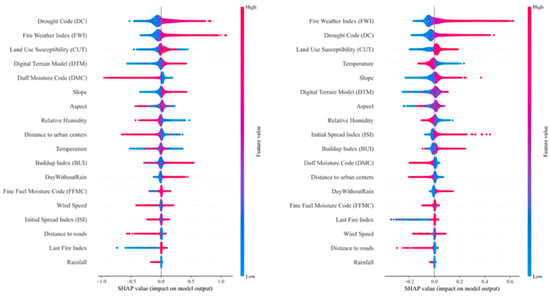
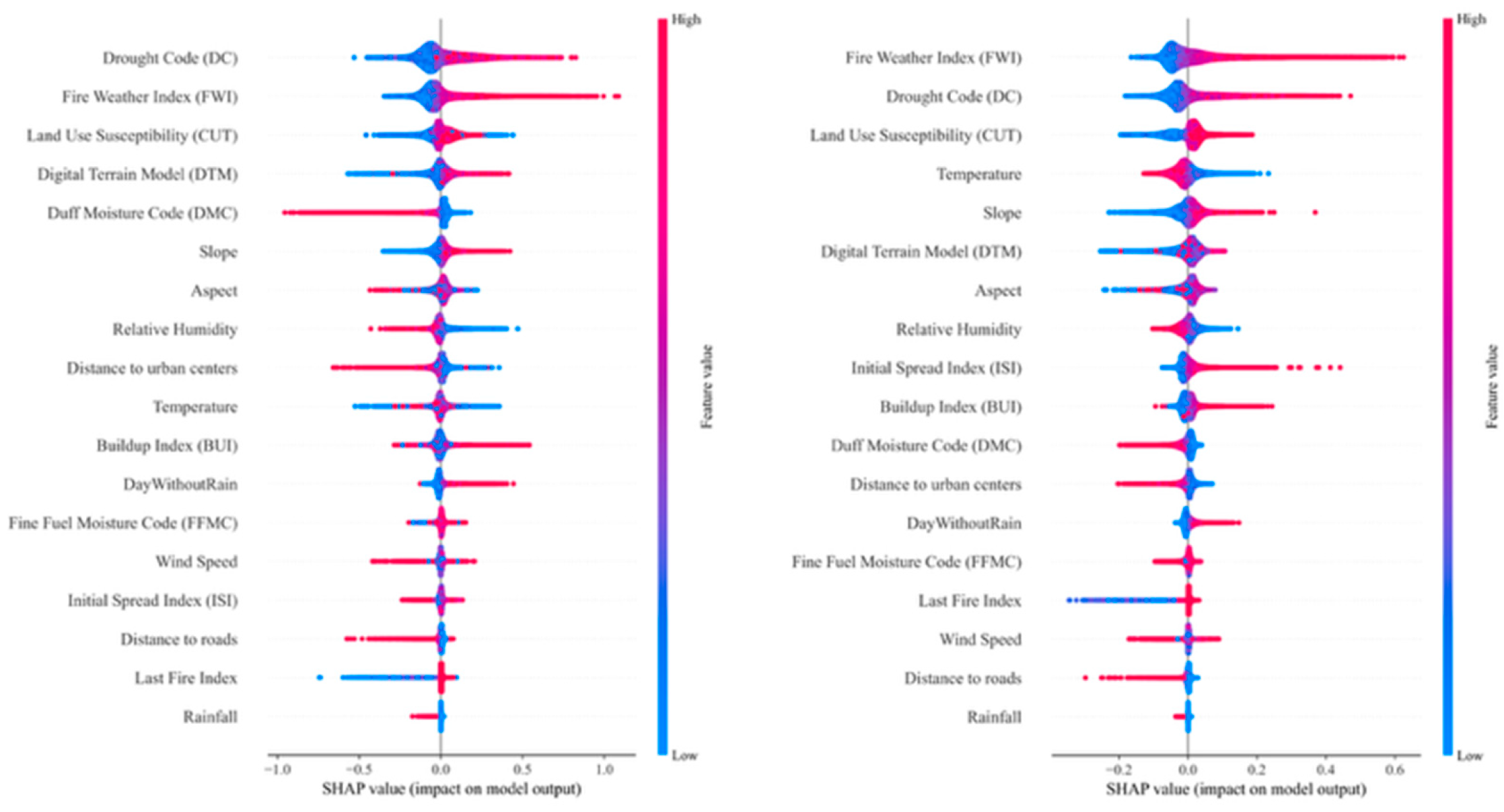
The SHAP analysis was used to quantify the contribution of each predictor in the Historical-ALL model for the two testing periods, TP1 and TP2 (Figure 7, left and right, respectively). In both periods, the most influential variables were the FWI and its sub-component DC, indicating that the model relies primarily on the overall fire-weather signal and on long-term fuel dryness. Static variables also play a substantial role, particularly land cover and the DTM, followed by aspect and slope; the network thus combines fire-weather conditions with the territory’s spatial characteristics, which the FWI alone cannot capture. The raw meteorological variables (temperature, wind speed, relative humidity and precipitation) contribute comparatively less, most likely because their information is already embedded in the FWI and its sub-components, which are computed from the same variables. Finally, shorter distances to roads and urban centers increase predicted susceptibility, confirming that the model links wildfire occurrence to proximity to human activity, consistent with the predominantly anthropogenic origin of ignitions in the Mediterranean area.
Figure 7.
The SHAP analysis of the WNN ALL-Historical configurations for the testing periods TP1 (2017–2018, left) and TP2 (2018, right).
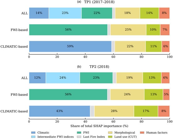
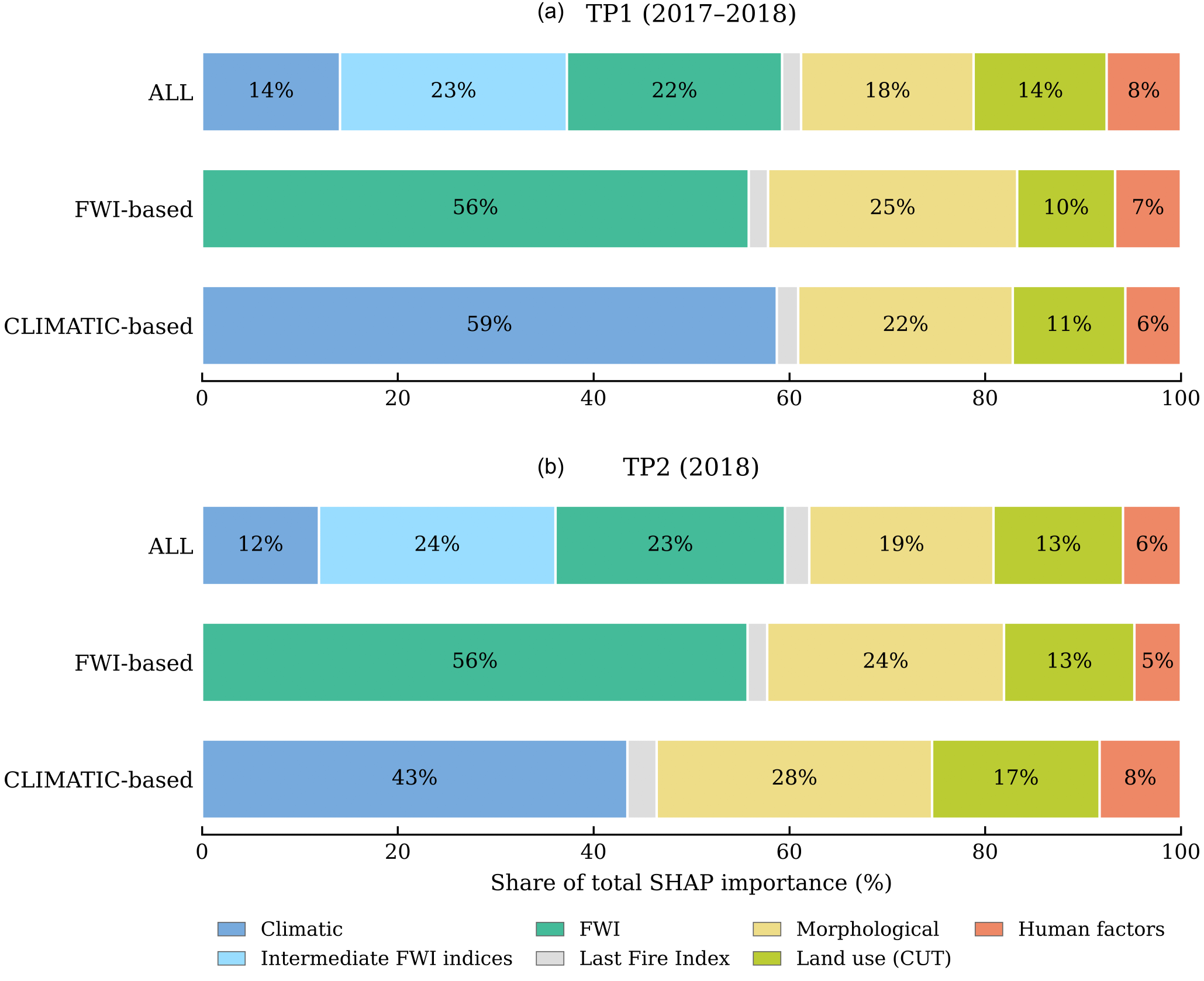
Regarding the importance of the predictor groups across the different model configurations, Figure 8 shows how the total SHAP importance is shared among the predictor groups in the three model configurations. Fire-weather information clearly dominated in all of them. In the Historical-ALL model, it accounted for 59% of the total in both test periods, divided almost equally between the FWI (22–23%) and its intermediate indices (23–24%), with a smaller share for the raw climatic variables (12–14%). When the FWI was the only weather input, as in the FWI-based model, it alone explained 56% of the output; when only raw climatic variables were available, they accounted for 59% in TP1 and 43% in TP2. In other words, the models rely on meteorological information to a broadly similar extent, whether this enters as raw variables or through the FWI system. This supports what emerged from the analysis of individual predictors (Figure 7): the modest contribution of the raw climatic variables in the Historical-ALL model does not mean that weather is unimportant, but that most of its signal is already carried by the FWI and its sub-components, which are derived from the same variables.
Figure 8.
Contribution of each predictor group to the output of the Historical ALL, FWI-based and CLIMATIC-based models, expressed as a percentage of the total SHAP importance, for (a) TP1 (2017–2018) and (b) TP2 (2018).
The rest of the explanation comes from static predictors. Morphology contributed between 18% and 28% of the total importance, land use between 10% and 17%, and human factors between 5% and 8%, whereas the Last Fire Index played only a marginal role (3% or less). For the Historical-ALL and FWI-based models, this picture hardly changed from TP1 to TP2. The CLIMATIC-based model behaved differently: in TP2, the weight of meteorological variables dropped from 59% to 43%, and morphology and land use made up the difference.
It should be noted that SHAP values describe how a trained model uses its inputs to produce its output, and not how much each predictor or group contributes to predictive skill. A predictor may receive a large SHAP importance without improving performance, for instance, when its information is redundant with that of other inputs. Moreover, when predictors are strongly correlated, as with the FWI components and the raw meteorological variables from which they are derived, the attribution among them is not uniquely defined and the model may split it arbitrarily. The SHAP shares reported in Figure 7 and Figure 8 should therefore be interpreted as a description of the internal functioning of each model, not as a performance attribution.
3.3. Map-Based Visual Assessment
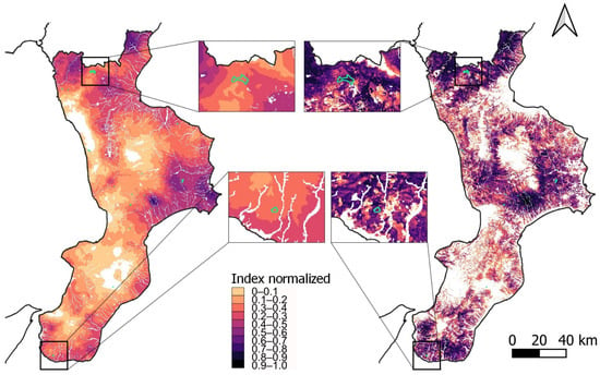
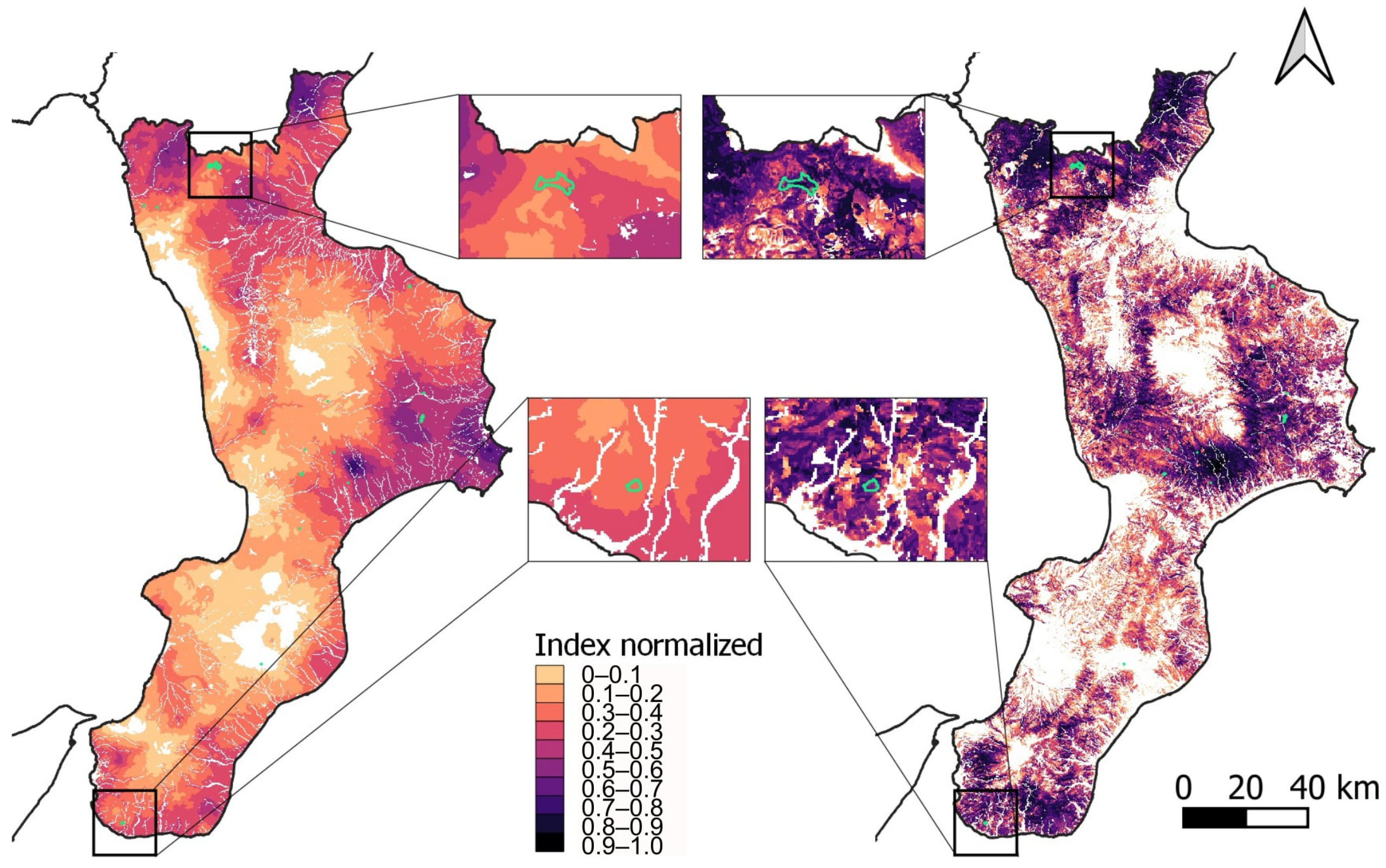
Figure 9 shows a visual comparison of the susceptibility maps produced by the FWI and WNN methods on 30 July 2017, an arbitrarily chosen sample day because of the high number of recorded wildfires. Due to the different outcome ranges of the two models, a preliminary normalization was necessary by keeping the spatial map resolution unchanged. To this end, a preliminary transformation to binary Foff/Fon maps was applied by using the ROC analysis and the geometric mean metric to find the monthly threshold values, calculated considering the training period, that optimally identify threshold values for distinguishing fire-prone and non-fire-prone conditions in the input maps [46]. As for FWI maps, the FWI monthly threshold was considered as the lower boundary, while the EFFIS FWI very extreme class threshold was the upper boundary (set to 70 in June 2021; https://forest-fire.emergency.copernicus.eu/about-effis/technical-background/fire-danger-forecast, accessed on 29 October 2026). The WNN map was normalized using the WNN monthly threshold and the maximum possible probability of 1. In both cases, the values were rescaled using min–max normalization: (x − min)/(max − min). To make the two models comparable, the minimum was defined with the same approach for both, while the maximum FWI value was taken from the literature. Sites below the minimum threshold are not shown in the figure (i.e., the corresponding pixels are white-shaded), even though the legend refers to the full range of normalized values. The maps show that the network better matched the actual fire events, delimited by green polygons in Figure 6. Indeed, real cases fell into the low classes (ranging from 0.2–0.3 and 0.3–0.4) for FWI and the high classes (0.8–0.9 and 0.9–1) for WNN. For the selected day, the WNN map assigned higher susceptibility values to several areas where fire events were observed, whereas the FWI map tended to distribute high values more smoothly over broader areas. This suggests that WNN provides a more spatially selective representation of fire-prone conditions.
Figure 9.
Comparison of FWI (left) and WNN (right) maps related to the prediction for 30 July 2017. The maps are subdivided into 10 susceptibility classes of equally distributed normalized probabilities. Green polygons circumscribe actual fire events. The white pixels represent values below the monthly thresholds for both FWI and WNN.
3.4. Shannon Entropy Assessment
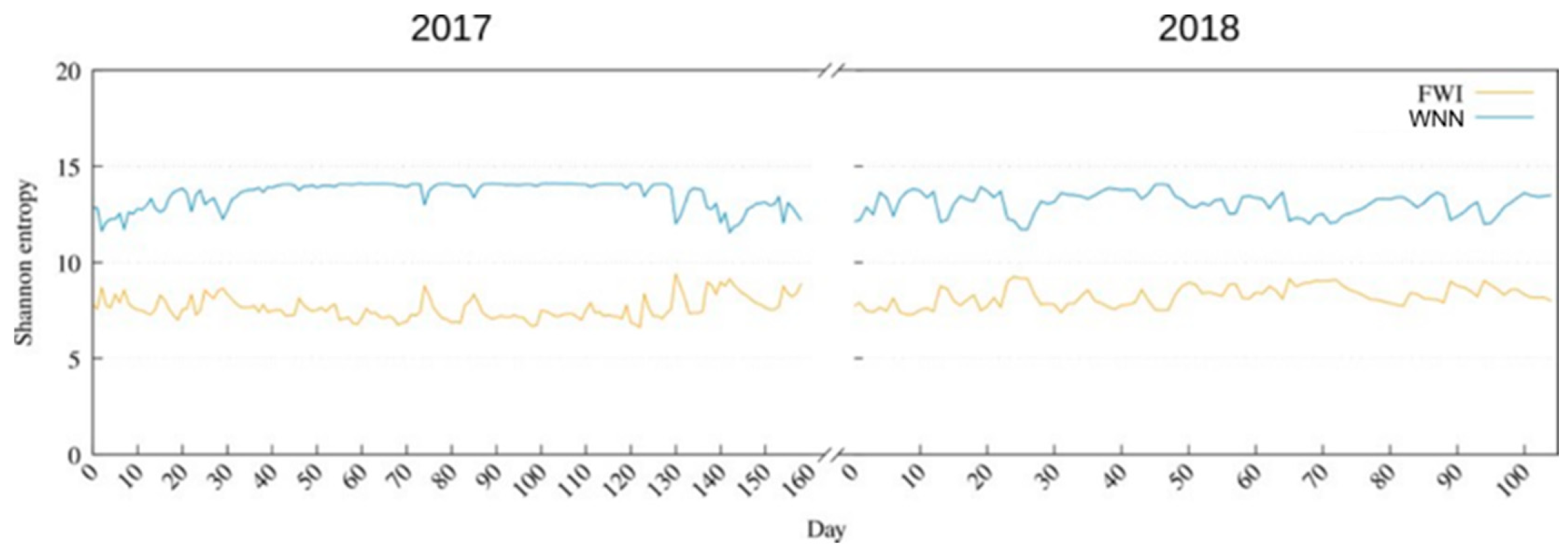
Visual inspection of Figure 9 suggests that WNN maps are more spatially differentiated than FWI maps. To quantify this, we computed the daily Shannon entropy [45] of each susceptibility map as a measure of its information content. Entropy is low when most pixels share the same or a few susceptibility values, so that the map poorly discriminates between areas, and increases as susceptibility values are spread over a wider range of levels across the territory. The concepts of entropy and information content are widely used to estimate the spatial distribution of variables (e.g., [47]). In this context, higher entropy therefore indicates a map that better differentiates areas within the region. This does not directly measure predictive accuracy, but it provides complementary information on the spatial variability and potential operational usefulness of the maps.
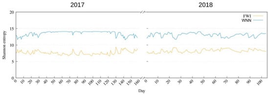
The result of the Shannon entropy analysis is shown in Figure 10. As can be seen, WNN consistently provided higher information and spatially distributed content with respect to FWI alone. On average, the Shannon entropy equaled 8.23 for FWI and 13.2 for WNN. Furthermore, the first part of the WNN Shannon entropy for 2017 was much more constant than for 2018. Such behavior could be possibly related to the generally drier and warmer climate in 2017 compared with 2018, which warrants further investigation and was beyond the scope of this study.
Figure 10.
Shannon entropy calculated for the 2017–2018 prediction. The x-axis shows the number of days with at least one fire.
3.5. Quantitative Assessment
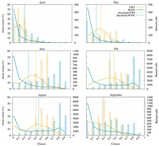
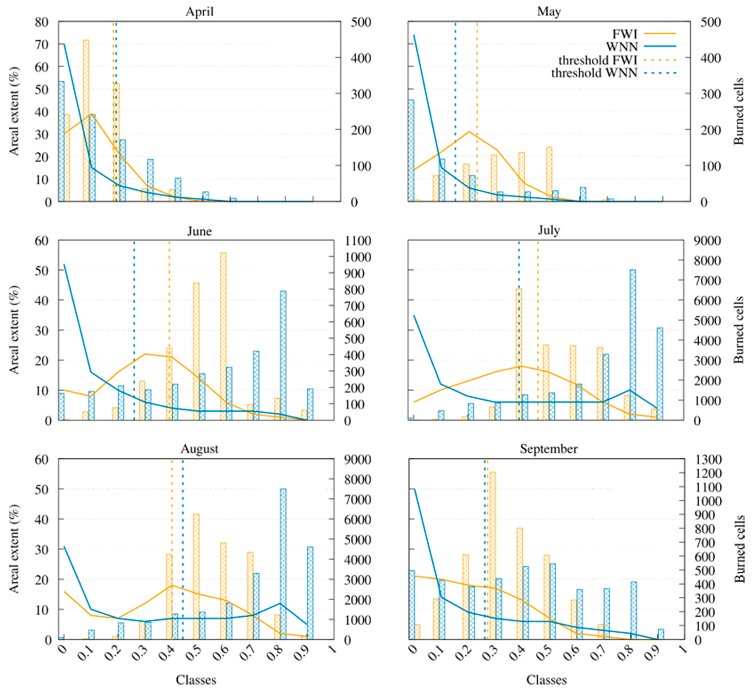
In addition to the above analyses, we conducted a further assessment by counting the number of real fire events (frequencies) intercepted by each susceptibility class in both the WNN and FWI maps during the test period from 2017 to 2018 (it is worth noting that 2017 was an exceptional year in terms of wildfire occurrence). Monthly-averaged values over the entire two-year period of analysis were considered. Results of this analysis are shown in Figure 11, which also depicts the extents of the susceptibility classes alongside the monthly thresholds. In April and May, most real events fell in the lower susceptibility classes for both WNN and FWI, below the monthly thresholds, resulting in poor predictive performance for both methods. The trends differed completely in June, July, and August, with the two models behaving very differently. Most real events fell in the intermediate FWI susceptibility classes, while WNN was more consistent because most real fires fell in the higher susceptibility classes. The trend was also more favorable for WNN, with an exponential-like monotone increase up to class [0.8,0.9), followed by a drop to class [0.9,1.0], while FWI peaked in correspondence with intermediate classes. Ultimately, September showed no clear trend, even though WNN maintained an advantage in predicting real events with high-value susceptibility classes.
Figure 11.
Areal extent in percentage (left y-axis, lines) and number of burned cells (right y-axis, histograms) plotted against the normalized index values for the 2017–2018 prediction maps. Lines show the percentage of the study area falling within each class; histograms show the number of burned cells falling within each class. Blue indicates the WNN results and yellow the FWI benchmark. Dashed vertical lines mark the monthly-averaged fire-susceptibility thresholds.
4. Discussion and Conclusions
This work introduced the WNN deep neural network model for wildfire susceptibility forecasting and demonstrated its operational readiness by applying it to the Calabria region, a Mediterranean hotspot for wildfire events, using data from 2010 to 2018. The proposed model uses a subset of the dataset from [11]: 17 out of the original 21 input variables and burned areas. Two learning periods, namely 2010–2016 and 2010–2017, were considered, with testing periods of 2017–2018 and only 2018, respectively. Two sampling strategies, one of which (named “historical”) took into consideration previous fire events in the study area, and three sets of input features extracted from a group of 18 variables were also considered, resulting in 12 training/testing experiments. Meteorological data were included in each set of input features in alternative ways: in their raw form, as FWI building blocks, and through the FWI index. Each tested set of input features also included geomorphological and land-use/land-cover variables, as well as human triggering factors.
The 12 experiments performed with WNN were compared with the FWI model using different methods, including confusion ROC and precision-recall analysis, SHAP analysis and feature importance, qualitative visual inspection of wildfire susceptibility maps, Shannon entropy analysis for assessing the level of maps’ information content, and a quantitative assessment in which we measured the agreement between the wildfire susceptibility classes and the observed fire events for the entire period of analysis. Overall, the specific WNN configuration combining the full set of 18 features (i.e., considering all the anthropogenic factors, the climatic-based, and FWI-derived features) with the historical sampling strategy was selected as the best among the tested alternatives due to both its strong AUROC and PR-AUC performance and its ability to leverage the additional year of training to predict 2018 fire behavior. The improved performance of the historical sampling strategy may partly reflect learning spatial fire recurrence, i.e., the tendency for fires to recur in previously burned cells, which random sampling cannot exploit. This effect should not be treated as entirely separate from susceptibility: recurrence largely results from persistent predisposing factors, such as vegetation type, terrain, and proximity to human activity, which themselves underlie susceptibility. However, part of the advantage may also stem from location-specific patterns that the model learns from past fire occurrence rather than from the predictors, and these patterns may not transfer to areas with no fire history. The skill of the historical configurations should therefore be interpreted as the combined effect of susceptibility and spatial persistence. Compared with the Fire Weather Index (FWI) method, WNN produced higher AUROC values, greater spatial information content, and more spatially selective susceptibility maps. Our work demonstrates that a deep learning (DL) approach can outperform a standard, globally adopted model in wildfire susceptibility mapping. Here, susceptibility is understood as a relative measure that discriminates the most fire-prone areas, thereby supporting prioritization and providing information that can be used at the various stages of wildfire management.
Critically, these gains are not confined to a research setting: the WNN model has already moved beyond proof-of-concept and is running operationally. It is integrated into the PANORAMA web platform as P-FireCast (https://panorama.cesmma.unical.it/user-area/map, last accessed 22 October 2026), where it ingests daily weather forecasts for the study area and generates high-resolution, 4-day lead-time wildfire susceptibility maps, updated daily. The weather forecasting system was developed by our research group and has been operational since January 2020, providing freely available forecasts updated daily. Though the quantitative assessment of the performance of the forecasting system will be accurately assessed in future work and is, anyway, beyond the scope of this paper, we would like to highlight its potential for supporting the deployment and pre-positioning of firefighting resources, given the demonstrated sharper spatial discrimination of more highly susceptible areas to fire.
The present study has some limitations. First, the validation is restricted to Calabria and to a relatively short independent testing period, particularly for the TP2 configuration. The approach’s transferability to other Mediterranean regions depends on the availability of observed data. In this work, we used high-quality observations of both wildfire on-field occurrence and meteorological variables, the latter from a dense monitoring network and interpolated following [11]; the same protocol would need to be extended to other regions. Moreover, an important limitation is the state of the vegetation (i.e., the fuel), which we treated as static over time. In reality, it is dynamic and can be represented using spectral vegetation indices derived from satellite imagery. Second, the anthropogenic component is represented through simple spatial proxies, such as distance to roads and urban centers, which cannot fully capture human ignition behavior. Third, the current feed-forward architecture does not explicitly model temporal dependence, although historical information is partly introduced through selected predictors and the sampling strategy. Finally, model interpretability remains limited and should be improved using more complex approaches. Building on its current operational status, this work can be extended in several directions. First, a leave-one-group-out ablation study could be conducted by retraining the network after removing one predictor group at a time and comparing it with the full model on the same test years to quantify each group’s contribution to predictive skill independently of the others. Second, recurrent neural networks, such as the LSTM (Long Short-Term Memory), could be applied to the feed-forward architecture considered here to better account for the history of events in the study area (e.g., [48,49]). Third, deep learning-based emulation of fire weather indices could be explored to better integrate meteorological drivers into the modeling framework [32]. In this sense, additional study periods and regions will be considered to further assess the proposed approach’s reliability in potential applications within operational risk management frameworks.
Author Contributions
Writing—original draft, A.D.R. and L.F.; Software, A.D.R.; Visualization, A.D.R. and L.F.; Conceptualization, A.S. and G.M.; Data curation, L.F. and A.D.R.; Funding Acquisition, G.M.; Investigation, A.D.R., D.D. and A.S.; Supervision, G.M. and A.S.; Writing—review and editing, all authors. All authors have read and agreed to the published version of the manuscript.
Funding
This work was funded by the Next Generation EU—Italian NRRP, Mission 4, Component 2, Investment 1.5, call for the creation and strengthening of “Innovation Ecosystems”, building “Territorial R&D Leaders” (Directorial Decree n. 2021/3277)—project Tech4You—Technologies for climate change adaptation and quality of life improvement, n. ECS0000009. This work reflects only the authors’ views and opinions; neither the Ministry for University and Research nor the European Commission can be considered responsible for them.
Data Availability Statement
This trained model is publicly available at https://github.com/alessioderango/WNN (accessed on 29 October 2026), while the already-processed data for reproducing the 2018 validation year are available at https://doi.org/10.5281/zenodo.21840359. The software is written in Python 3, and the required packages are provided through the conda environment available on the GitHub repository. For any inquiries, please contact PhD Alessio De Rango (alessio.derango@unical.it).
Conflicts of Interest
The authors declare no conflicts of interest.
Abbreviations
The following abbreviations are used in this manuscript:
| WNN | Wildfire Neural Network |
| FWI | Fire Weather Index |
| tdry | The number of days without rain |
| DC | Drought Code |
| DMC | Duff Moisture Code |
| FFMC | Fine Fuel Moisture Code |
| ISI | Initial Spread Index |
| BUI | Buildup Index |
| tlf | The number of days since the last fire event |
| CUT | Land Use Susceptibility |
| DTM | Digital Terrain Model |
| AUROC | Area Under the ROC Curve |
| PR-AUC | Precision—Recall Area Under the Curve |
References
- Sousa-Lima, L.V.; Saggioro, E.M.; Dorneles, P.R.; Parente, C.E.T. Fire on the Ground: Wildfires Impacts on Soil Health and Biodiversity—A Review. Sci. Total Environ. 2025, 1004, 180725. [Google Scholar]
- McGuire, L.A.; Ebel, B.A.; Rengers, F.K.; Vieira, D.C.S.; Nyman, P. Fire Effects on Geomorphic Processes. Nat. Rev. Earth Environ. 2024, 5, 486–503. [Google Scholar] [CrossRef] [Scilit]
- Reid, C.E.; Brauer, M.; Johnston, F.H.; Jerrett, M.; Balmes, J.R.; Elliott, C.T. Critical Review of Health Impacts of Wildfire Smoke Exposure. Environ. Health Perspect. 2016, 124, 1334–1343. [Google Scholar] [CrossRef] [Scilit]
- Gould, C.F.; Heft-Neal, S.; Johnson, M.; Aguilera, J.; Burke, M.; Nadeau, K. Health Effects of Wildfire Smoke Exposure. Annu. Rev. Med. 2024, 75, 277–292. [Google Scholar] [CrossRef] [Scilit]
- Ali, E.; Cramer, W.; Carnicer, J.; Georgopoulou, E.; Hilmi, N.J.M.; Le Cozannet, G.; Lionello, P. Cross-Chapter Paper 4: Mediterranean Region. In Climate Change 2022: Impacts, Adaptation and Vulnerability. Contribution of Working Group II to the Sixth Assessment Report of the Intergovernmental Panel on Climate Change; Pörtner, H.-O., Roberts, D.C., Tignor, M., Poloczanska, E.S., Mintenbeck, K., Alegría, A., Craig, M., Langsdorf, S., Löschke, S., Möller, V., et al., Eds.; Cambridge University Press: Cambridge, UK; New York, NY, USA, 2022; pp. 2233–2272. [Google Scholar]
- Ghasemiazma, F.; Tonini, M.; Fiorucci, P.; Turco, M. Megafires in Mediterranean Europe: The Compound Role of Fire Weather and Drought. npj Nat. Hazards 2026, 3, 33. [Google Scholar] [CrossRef] [Scilit]
- San-Miguel-Ayanz, J.; Durrant, T.; Boca, R.; Maianti, P.; Liberta, G.; Oom, D.; Branco, A.; De Rigo, D.; Suarez, M.M.; Ferrari, D.; et al. Advance Report on Forest Fires in Europe, Middle East and North Africa 2024; EUR 40255, JRC141505; Publications Office of the European Union: Luxembourg, 2025. [Google Scholar]
- El Garroussi, S.; Di Giuseppe, F.; Barnard, C.; Wetterhall, F. Europe Faces up to Tenfold Increase in Extreme Fires in a Warming Climate. npj Clim. Atmos. Sci. 2024, 7, 30. [Google Scholar] [CrossRef] [Scilit]
- Mendicino, G.; Versace, P. Integrated Drought Watch System: A Case Study in Southern Italy. Water Resour. Manag. 2007, 21, 1409–1428. [Google Scholar] [CrossRef] [Scilit]
- Senatore, A.; Fuoco, D.; Maiolo, M.; Mendicino, G.; Smiatek, G.; Kunstmann, H. Evaluating the Uncertainty of Climate Model Structure and Bias Correction on the Hydrological Impact of Projected Climate Change in a Mediterranean Catchment. J. Hydrol. Reg. Stud. 2022, 42, 101120. [Google Scholar] [CrossRef] [Scilit]
- De Rango, A.; Lo Scudo, F.; Furnari, L.; Senatore, A.; D’Ambrosio, D.; Mendicino, G.; Greco, G. CalWildFire: A High-Resolution In Situ Dataset for Wildfire Analysis and Modeling in the Mediterranean Region. Sci. Data 2026, 13, 859. [Google Scholar] [CrossRef] [Scilit]
- Castagna, J.; Senatore, A.; Bencardino, M.; D’Amore, F.; Sprovieri, F.; Pirrone, N.; Mendicino, G. Multiscale Assessment of the Impact on Air Quality of an Intense Wildfire Season in Southern Italy. Sci. Total Environ. 2021, 761, 143271. [Google Scholar] [CrossRef] [Scilit]
- Van Wagner, C.E. Development and Structure of the Canadian Forest Fire Weather Index System; Canadian Forestry Service: Ottawa, ON, Canada, 1987.
- Colosimo, F.; Maletta, R.; Mendicino, G.; Siviglia, S. Foreste, Prevenzione Dagli Incendi e Sicurezza Ambientale; Rubettino: Soveria Mannelli, Italy, 2021. (In Italian) [Google Scholar]
- Jiang, R.; Cai, Z.; Wang, Z.; Yang, C.; Fan, Z.; Chen, Q.; Song, X.; Shibasaki, R. Predicting Citywide Crowd Dynamics at Big Events: A Deep Learning System. ACM Trans. Intell. Syst. Technol. 2022, 13, 21. [Google Scholar] [CrossRef] [Scilit]
- Jupalle, H.; Kouser, S.; Bhatia, A.B.; Alam, N.; Nadikattu, R.R.; Whig, P. Automation of Human Behaviors and Its Prediction Using Machine Learning. Microsyst. Technol. 2022, 28, 1879–1887. [Google Scholar] [CrossRef] [Scilit]
- Jain, P.; Coogan, S.C.; Subramanian, S.G.; Crowley, M.; Taylor, S.; Flannigan, M.D. A Review of Machine Learning Applications in Wildfire Science and Management. Environ. Rev. 2020, 28, 478–505. [Google Scholar] [CrossRef] [Scilit]
- Xu, R.; Lin, H.; Lu, K.; Cao, L.; Liu, Y. A Forest Fire Detection System Based on Ensemble Learning. Forests 2021, 12, 217. [Google Scholar] [CrossRef] [Scilit]
- De Rango, A.; Furnari, L.; Cortale, F.; Senatore, A.; Mendicino, G. Wildfire Early Warning System Based on a Smart CO2 Sensors Network. Sensors 2025, 25, 2012. [Google Scholar] [CrossRef] [Scilit]
- Ali, A.W.; Kurnaz, S. Optimizing Deep Learning Models for Fire Detection, Classification, and Segmentation Using Satellite Images. Fire 2025, 8, 36. [Google Scholar] [CrossRef] [Scilit]
- Naderpour, M.; Mojaddadi Rizeei, H.; Ramezani, F. Forest Fire Risk Prediction: A Spatial Deep Neural Network-Based Framework. Remote Sens. 2021, 13, 2513. [Google Scholar] [CrossRef] [Scilit]
- Zhang, G.; Wang, M.; Liu, K. Deep Neural Networks for Global Wildfire Susceptibility Modelling. Ecol. Indic. 2021, 127, 107735. [Google Scholar] [CrossRef] [Scilit]
- Di Giuseppe, F.; McNorton, J.; Lombardi, A.; Wetterhall, F. Global Data-Driven Prediction of Fire Activity. Nat. Commun. 2025, 16, 2918. [Google Scholar] [CrossRef] [Scilit]
- Hodges, J.L.; Lattimer, B.Y. Wildland Fire Spread Modeling Using Convolutional Neural Networks. Fire Technol. 2019, 55, 2115–2142. [Google Scholar] [CrossRef] [Scilit]
- Allaire, F.; Mallet, V.; Filippi, J.-B. Emulation of Wildland Fire Spread Simulation Using Deep Learning. Neural Netw. 2021, 141, 184–198. [Google Scholar] [CrossRef] [Scilit]
- Moradpour, M.; Kumar, P.; Hoshyaripour, G.A. Convolutional Neural Networks for Wildfire Spread and Intensity Prediction. Appl. Comput. Geosci. 2026, 30, 100355. [Google Scholar] [CrossRef] [Scilit]
- Cilli, R.; Elia, M.; D’Este, M.; Giannico, V.; Amoroso, N.; Lombardi, A.; Pantaleo, E.; Monaco, A.; Sanesi, G.; Tangaro, S.; et al. Explainable Artificial Intelligence (XAI) Detects Wildfire Occurrence in the Mediterranean Countries of Southern Europe. Sci. Rep. 2022, 12, 16349. [Google Scholar] [CrossRef] [Scilit]
- Trucchia, A.; Meschi, G.; Fiorucci, P.; Gollini, A.; Negro, D. Defining Wildfire Susceptibility Maps in Italy for Understanding Seasonal Wildfire Regimes at the National Level. Fire 2022, 5, 30. [Google Scholar] [CrossRef] [Scilit]
- Piralilou, S.T.; Einali, G.; Ghorbanzadeh, O.; Nachappa, T.G.; Gholamnia, K.; Blaschke, T.; Ghamisi, P. A Google Earth Engine Approach for Wildfire Susceptibility Prediction Fusion with Remote Sensing Data of Different Spatial Resolutions. Remote Sens. 2022, 14, 672. [Google Scholar] [CrossRef] [Scilit]
- Kondylatos, S.; Prapas, I.; Ronco, M.; Papoutsis, I.; Camps-Valls, G.; Piles, M.; Fernández-Torres, M.; Carvalhais, N. Wildfire Danger Prediction and Understanding with Deep Learning. Geophys. Res. Lett. 2022, 49, e2022GL099368. [Google Scholar] [CrossRef] [Scilit]
- Apostolakis, A.; Girtsou, S.; Giannopoulos, G.; Bartsotas, N.S.; Kontoes, C. Estimating Next Day’s Forest Fire Risk via a Complete Machine Learning Methodology. Remote Sens. 2022, 14, 1222. [Google Scholar] [CrossRef] [Scilit]
- Mirones, Ó.; Bedia, J.; Soares, P.M.M.; Gutiérrez, J.M.; Baño-Medina, J. Deep Learning Emulation of Multivariate Climate Indices: A Case Study of the Fire Weather Index in the Iberian Peninsula. Nat. Hazards Earth Syst. Sci. 2026, 26, 3417–3442. [Google Scholar] [CrossRef] [Scilit]
- Granata, F.; Di Nunno, F. Advancing Fire Weather Forecasting: Deep Learning with Kolmogorov–Arnold and Fourier Networks across Italy. Nat. Hazards 2026, 122, 58. [Google Scholar] [CrossRef] [Scilit]
- Federico, S.; Pasqualoni, L.; Avolio, E.; Bellecci, C. Brief Communication “Calabria Daily Rainfall from 1970 to 2006”. Nat. Hazards Earth Syst. Sci. 2010, 10, 717–722. [Google Scholar] [CrossRef] [Scilit]
- Bedia, J.; Herrera García, S.; Camia, A.; Moreno, J.; Gutiérrez, J. Forest Fire Danger Projections in the Mediterranean Using Ensembles Regional Climate Change Scenarios. Clim. Change 2014, 122, 185–199. [Google Scholar] [CrossRef] [Scilit]
- Spampinato, G.; Crisarà, R.; Cameriere, P.; Cano-Ortiz, A.; Musarella, C.M. Analysis of the Forest Landscape and Its Transformations through Phytotoponyms: A Case Study in Calabria (Southern Italy). Land 2022, 11, 518. [Google Scholar] [CrossRef] [Scilit]
- Büttner, G.; Feranec, J.; Jaffrain, G.; Mari, L.; Maucha, G.; Soukup, T. The Corine Land Cover 2000 Project. EARSeL eProc. 2004, 3, 331–346. [Google Scholar]
- Calabria Region. Carta Usi del Territorio—Land Use Classification; Regione Calabria: Catanzaro, Italy, 2020.
- Bertani, R.; Bovio, G.; Petrucci, B. Manuale per l’Applicazione dello "Schema di Piano A.I.B. nei Parchi Nazionali"—2018; Ministero dell’Ambiente e della Tutela del Territorio e del Mare: Rome, Italy, 2018. (In Italian)
- Blasi, C.; Bovio, G.; Corona, P.; Marchetti, M.; Maturani, A. Incendi e Complessità Ecosistemica. Dalla Pianificazione Forestale al Recupero Ambientale; Ministero dell’Ambiente e della Tutela del Territorio, Società Botanica Italiana; Palombi: Rome, Italy, 2004. (In Italian) [Google Scholar]
- Kingma, D.P.; Ba, J. Adam: A Method for Stochastic Optimization. arXiv 2014, arXiv:1412.6980. [Google Scholar]
- Goodfellow, I.; Bengio, Y.; Courville, A. Deep Learning; MIT Press: Cambridge, MA, USA, 2016; Available online: http://www.deeplearningbook.org (accessed on 29 October 2026).
- Hinton, G.; Srivastava, N.; Krizhevsky, A.; Sutskever, I.; Salakhutdinov, R. Dropout: A Simple Way to Prevent Neural Networks from Overfitting. J. Mach. Learn. Res. 2014, 15, 1929–1958. [Google Scholar]
- Zhang, G.; Wang, M.; Liu, K. Forest Fire Susceptibility Modeling Using a Convolutional Neural Network for Yunnan Province of China. Int. J. Disaster Risk Sci. 2019, 10, 386–403. [Google Scholar] [CrossRef] [Scilit]
- Shannon, C.E.; Weaver, W. The Mathematical Theory of Communication; University of Illinois Press: Urbana, IL, USA, 1949. [Google Scholar]
- Brownlee, J. Imbalanced Classification with Python: Better Metrics, Balance Skewed Classes, Cost-Sensitive Learning; Machine Learning Mastery: Vermont, Australia, 2020. [Google Scholar]
- Mendicino, G.; Sole, A. The Information Content Theory for the Estimation of the Topographic Index Distribution Used in TOPMODEL. Hydrol. Process. 1997, 11, 1099–1114. [Google Scholar] [CrossRef] [Scilit]
- Bahadori, N.; Razavi-Termeh, S.V.; Sadeghi-Niaraki, A.; Al-Kindi, K.M.; Abuhmed, T.; Nazeri, B.; Choi, S.-M. Wildfire Susceptibility Mapping Using Deep Learning Algorithms in Two Satellite Imagery Dataset. Forests 2023, 14, 1325. [Google Scholar] [CrossRef] [Scilit]
- Hu, P.; Tanchak, R.; Wang, Q. Developing Risk Assessment Framework for Wildfire in the United States—A Deep Learning Approach to Safety and Sustainability. J. Saf. Sci. Resil. 2024, 5, 23–32. [Google Scholar]

Disclaimer/Publisher’s Note: The statements, opinions and data contained in all publications are solely those of the individual author(s) and contributor(s) and not of MDPI and/or the editor(s). MDPI and/or the editor(s) disclaim responsibility for any injury to people or property resulting from any ideas, methods, instructions or products referred to in the content. |
© 2026 by the authors. Licensee MDPI, Basel, Switzerland. This article is an open access article distributed under the terms and conditions of the Creative Commons Attribution (CC BY) license.