


Abstract
This paper presents a conducting-channel model aimed at elucidating the generation of high-energy particles within a plasma chamber. Initially, the chamber is charged with neutral hydrogen gas at a density of approximately ~3.3 × 10²²/m3, equivalent to 1 torr at 300 K under ideal gas conditions. A Townsend discharge (dark discharge), driven by an externally imposed electric potential (500–1000 V) across the cathode and anode, is utilized to induce partial ionization of the hydrogen gas. Once a stable conducting channel with a high conductivity is established, a low electric potential (e.g., 100–500 V) is introduced to sustain the current in the conducting channel. Our investigation then delves into the impact of a high-emissivity cathode, such as lanthanum hexaboride (LaB6), on an arc discharge. We develop a theoretical model of the conducting channel that may emerge under these conditions. As the cathode surface heats, thermionic electrons form a localized layer of negative charge density outside the cathode, leading to an electric potential dip. Our multi-fluid simulations reveal the emergence of an electron-ion two-stream instability owing to the high-density electron layer, leading to the appearance of multiple potential peaks and dips, each measuring several to tens of kV. We delineate a set of conditions conducive to the formation of these potential peaks and dips within the conducting channel. Our proposed scenario furnishes a framework for elucidating electron and ion acceleration within a weakly ionized plasma chamber.
1. Introduction
The electron-ion two-stream instability, a fundamental plasma instability, arises when electrons and ions flow past each other at a relative velocity exceeding their thermal speeds. This relative drift transfers kinetic energy to charge separation and leads to the enhancement of particle speeds and electric potential [1,2]. In addition, the electric double layers [1,2,3,4,5] can also cause similar effects. The formation of localized electrostatic structures—whether quasi-static double layers (DLs) sustained by charge separation, or dynamically evolving potential oscillations driven by beam-plasma instabilities—represents one of the most fundamental and far-reaching phenomena in plasma physics. Such structures arise in laboratory discharges, space plasmas, and astrophysical environments, and they play a decisive role in particle acceleration, energy transport, and plasma confinement. The three processes reviewed here span three distinct physical regimes: current-free expanding plasmas [1,2], current-driven glow discharges [4], and beam-plasma instabilities in bounded systems [5]. Together, they provide a cohesive picture of how electric potential is built up, sustained, and modified across a wide range of plasma conditions. Hairapetian and Stenzel [1,2] demonstrated that a two-electron-temperature plasma expanding into vacuum naturally forms a current-free double layer with a potential drop of a few to tens of eV, scaling with the hot electron temperature. Conde and León [4] showed that in a glow discharge, multiple successive double layers each carry a quantized potential drop near the argon ionization potential (~15.76 V), yielding cumulative anode potentials of 30–50 V. Kaganovich and Sydorenko [5] revealed that in a bounded beam-plasma system, two-stream instability-driven electric potential oscillations can attain saturation amplitudes exceeding those of infinite plasmas by more than an order of magnitude due to boundary-induced mode selection. Together, these results not only deepen the fundamental understanding of plasma electrodynamics but also provide direct benchmarks for models of particle acceleration in laboratory, space, and technological plasma environments.
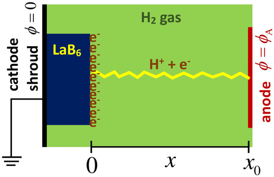
We consider a gas plasma chamber as shown in Figure 1. The chamber is filled with hydrogen gas at a density of ~. An arc discharge is triggered in the chamber. A cathode with high electron emissivity, such as lanthanum hexaboride (LaB6), is used. After a stable discharge is established with a higher potential (~500–1000 V) provided by the power supply, an electric potential V of ~100 V is imposed across the cathode and anode to maintain the current I in the conducting channel. The LaB6 cathode slab is heated and emits electrons, forming an electron layer and a potential dip around it. This potential dip can accelerate charge particles.
Figure 1.
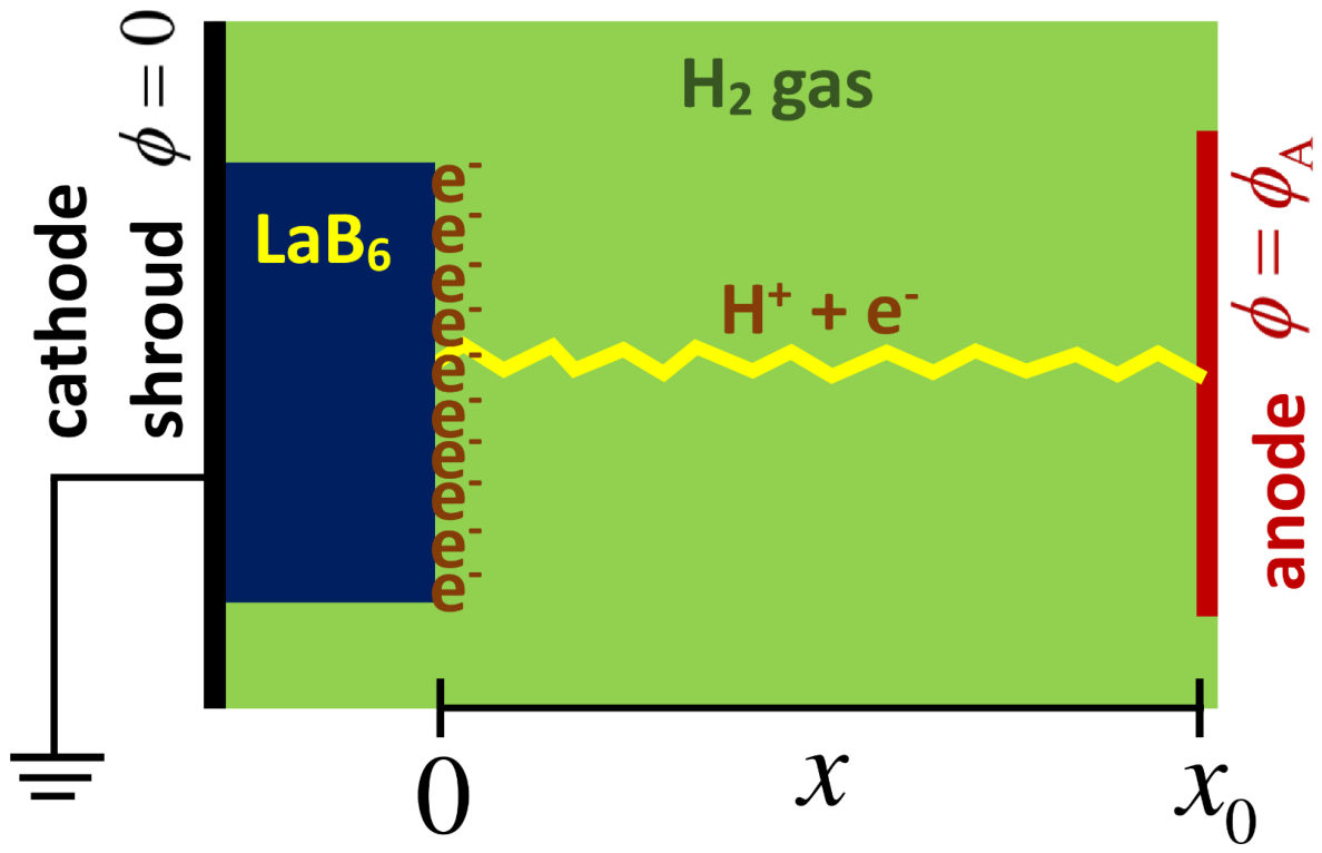
Schematic illustration of the simulation domain in part of the plasma chamber. The left-hand side is the LaB6 slab as cathode at 0 volt, and the right-hand side is the anode at a given potential 30 volts. The LaB6 slab is placed in a chamber filled with hydrogen gas . The gas pressure is maintained at 3–5 torr. The current flows from the anode to the LaB6 cathode. The yellow route between the LaB6 slab and anode is a conducting channel.
We note that to establish an arc discharge, a voltage of hundreds to thousands of volts is required to initialize the spark [6]. A stable arc current can then be formed with a high conductivity in the tube and maintained by a low voltage of ~100 volts with a current of a few to tens of amps [7,8]. The stable arc discharge is then maintained. The proposed theoretical model is based on the assumption that an arc discharge is maintained by an externally imposed electric potential (100–500 V) across the cathode and anode in the gas chamber. Recent progress on arc discharges has been reported [9,10,11,12,13] and a review article by Anders [14]. These studies provide a comprehensive view of plasma arcs and their interactions with metal, bridging the gap between specific, localized behaviors and broad, unifying frameworks. While the studies [9,10,11,12,13] detail complex, localized physics including chemical layer formation [9], heat transfer inaccuracies [10], tungsten tip melting [11], and energy radiation [13]. The framework by Anders [14] unites these studies and classifies different arc regimes.
It will be illustrated in this study that the applied voltage between the cathode (LaB6) and the anode is only from 100 V to 500 V, but the potential dips and peaks formed in the chamber can be tens of kV. The proposed mechanism can be applied to particle acceleration in a weakly ionized plasma or during a gas discharge.
A key finding demonstrated in this study is that while the externally applied bias between the cathode (LaB6) and the anode remains modest (100–500 V), the dynamically formed potential dips and peaks within the chamber can scale up to tens of kilovolts (kV). This proposed self-consistent voltage-amplification mechanism offers a novel framework for particle acceleration within weakly ionized plasmas or during intense gas discharges. Notably, analogous mechanisms involving the acceleration of ions and neutrals in rotating plasmas have been previously investigated for potential applications in controlled nuclear fusion [15,16,17]. In such fusion devices (e.g., magnetic mirrors or rotating plasma traps), achieving sufficient thermonuclear reaction rates requires ions to be accelerated to energies capable of overcoming the Coulomb barrier. By generating these high-energy particle beams through intrinsic plasma instabilities rather than relying entirely on massive external power grids, this mechanism provides a highly efficient pathway for non-thermal ion heating and acceleration in advanced fusion concepts. Furthermore, this laboratory configuration exhibits a strong phenomenological parallel to large-scale atmospheric discharge events, such as cloud-to-ground (CG) lightning driven by negatively or positively charged cloud bases. Section 5.2 presents a more detailed discussion on the lightning process.
2. Theoretical Model
In the proposed theoretical model, the plasma chamber is first imposed for demonstration with a voltage of 100 V across the anode and cathode (LaB6). A part of the chamber is shown in Figure 1. In the previous studies [16,17], the acceleration of ions and neutrals in a rotating plasma was studied for a potential application to nuclear fusion. The chamber is filled with hydrogen molecule (H2) gas with number density ~, corresponding to 1 torr at 300 K for an ideal gas. In our numerical simulations, the chamber pressure with is also used. The heated LaB6 slab can emit electrons. We note that the study in this paper is based on the assumption that an arc discharge with a small diameter is pre-established between the cathode and anode. It is similar to a gas-discharge lamp [7,8] except that in the proposed model, a good electron emitter, LaB6, is used as the cathode. Electrons emitted from the LaB6 cathode surface can form a potential dip, leading to plasma instability, as discussed later.
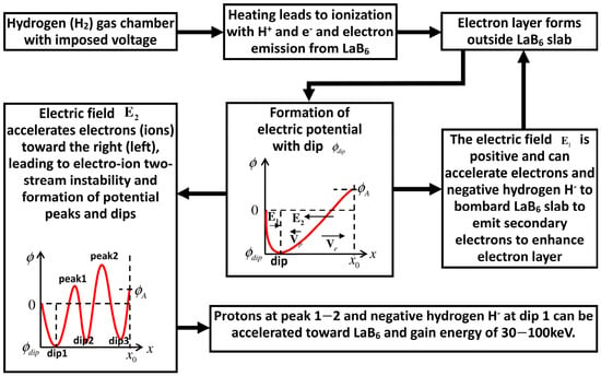
The physical process in the present theoretical model is illustrated in the flowchart in Figure 2. The externally imposed electric potential (V) leads to the formation of partially ionized hydrogen gas. As the LaB6 slab is heated, the emitted electrons from the LaB6 slab form a layer of negative charge density. The net negative charge density leads to a large electrostatic potential well near the surface of LaB6 slab with a potential dip at . In the quasi-neutral region slightly away from the LaB6 slab and the electron layer, the electric potential increases toward the anode, and the electrons and ions are accelerated in opposite directions, which leads to the electron-ion two-stream instability to be discussed later. This instability excites strong electrostatic waves, whose amplitudes may reach tens of kilovolts (kV), resulting in multiple potential dips and peaks.
Figure 2.
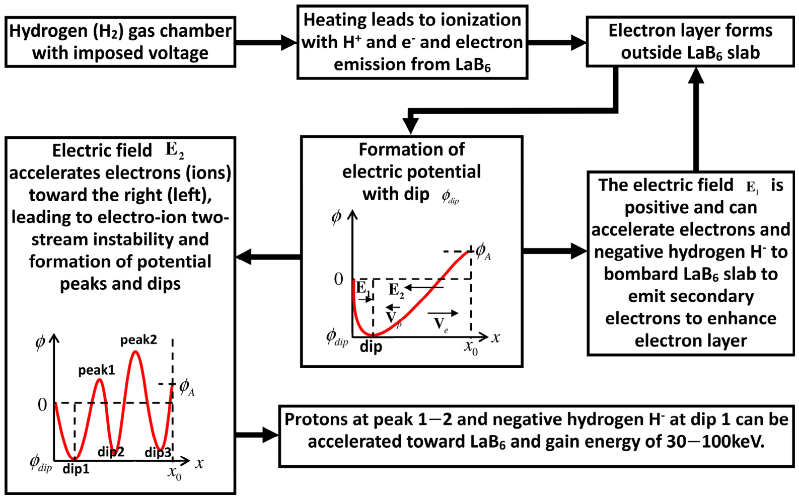
Flowchart for the formation of potential peaks and dips in the plasma chamber. The externally imposed electric potential (V) leads to the formation of partially ionized hydrogen gas. As the LaB6 slab is heated, the emitted electrons from the LaB6 slab form a layer of negative charge density. The electron layer together with the imposed voltage across the plasma chamber can lead to large electrostatic potential dips and peaks as illustrated in the chart based on multi–fluid simulations. The wavy potential structure may last for a few to tens of ns. The number of peaks and dips depends on the plasma density and electron velocity.
3. Simulation for the Formation of Potential Dips and Potential Peaks Generated by the Electron Layer in the Plasma Chamber
We perform multi-fluid simulations to study plasma dynamics and particle acceleration, and to investigate the formation of potential dips and peaks during an arc discharge in a plasma chamber. The initial condition of the simulation corresponds to a stable arc discharge that has already ionized the gas. We note that establishing an arc discharge requires a voltage of hundreds to thousands of volts to initiate the spark. A stable arc current can then be formed and maintained at a low voltage (e.g., 100 volts) with a current of a few to tens of amperes. The stable arc discharge is then used as the initial condition.
We set the cathode electric potential at zero volts and the anode electric potential of 100, 300, or 500 volts as the simulation boundary condition. The externally imposed potential is a time-independent boundary condition and is used for solving the one-dimensional electrostatic Poisson’s equation by using the tridiagonal matrix algorithm. It is similar to the formation of a conducting channel (return stroke) in gas-discharge lamps or in the air before the occurrence of lightning. It should be noted that the kink/sausage modes with their two-dimensional structure cannot occur in the one-dimensional approximation. In the proposed model, the emitted electrons at the cathode surface could further lead to the two-stream instability.
Figure 1 illustrates the simulation domain and setup. The left-hand side () is the LaB6 slab (cathode) with , and the right-hand side () is the anode with . The distance between the cathode and the anode is . The LaB6 slab is placed in a chamber filled with hydrogen gas, H2. The current flows from the anode to the LaB6 cathode. The hydrogen gas is heated and partially ionized, leading to the formation of plasma with H+ and e−.
3.1. The Governing Equations
The discharge and current flow are mostly aligned along this thin, elongated conducting tube. Hence, we simplify the key physical process into a one-dimensional problem, similar to the approach for the conducting channel associated with lightning [18]. Under this approximation, we developed a one-dimensional multi-fluid simulation code along the x-axis to study the formation of the electrostatic potential in the arc discharge. The governing equations are Poisson’s equation in electrostatics:
the continuity equation:
the momentum equation:
and the ideal gas law:
where e is the fundamental charge or Coulomb, is vacuum permittivity, and is charge density. The subscript indicates fluid species and can be electron (e) and proton (p), and the subscript “n” stands for “neutral”. The fluid quantities are number density n, velocity , pressure p, the Boltzmann constant J/K, charge q, electric field E, collision frequency for charge particles to neutral and temperature T. The real proton to electron mass ratio is used . The diffusion of electron and ion velocities through viscosity will be included and discussed later.
In this paper, we use a three-fluid (electron, ion, and neutral) simulation. The electron and the ion are independent, with their own continuity equations and momentum equations. The quasi-neutrality is not assumed and not required.
In the simulation with the complete energy equation, we found that the arc plasma can be quickly heated to well above 1 eV. However, the plasma can be partially converted to other parts of the chamber, which lowers the plasma temperature in the conducting channel. The radiation loss also reduces the plasma temperature. The temperature of the plasma in the region where current flows through is estimated to be 6000 K [19]. The simulation initial condition at t = 0 corresponds to the time when the arc discharge is formed, and the plasma is heated to We consider that the heating of the arc plasma from electricity and the heat loss through radiation and convection reach equilibrium during the simulation and that the temperature also reaches equilibrium in the conducting channel, which likely leads to constant temperature for all species .
We have tried a different system length ranging from 2 to 50 mm, and the length can affect the stability of the simulation and the formation of electrostatic waves. In this paper, we present the results associated with the system length of 2 mm, 5 mm, 8 mm, 10 mm, 20 mm, 30 mm, 40 mm, and 50 mm. In the simulations, the length x is normalized by . The other normalization parameters are neutral number density for and , electric potential 1 volt, velocity m/s (velocity of 1 eV proton) and time . For , . The numerical time step and grid spacing are and . The neutrals in the conducting tube are assumed to be heated from 300 K to 6000 K. With a constant pressure across the chamber, the density in the conducting channel will be reduced as one-twentieth of .
The numerical time step was chosen to resolve the fastest physical time scale in the system. In the present simulations, the electron plasma frequency is on the order of Hz. In addition, the electron-neutral and proton-neutral collision frequencies are on the order of Hz and Hz, respectively. Therefore, the adopted time step, , is sufficiently small to resolve both the plasma oscillation time scale and the charge-neutral collision time scales. For example, when , s, and thus , which is much smaller than , and .
The grid spacing is selected based on our numerical experience with this model. To check the effect of grid resolution, we also repeat representative simulations using 1024 grid points. The main results, including the formation of the potential dip near the cathode and the subsequent potential peaks and dips caused by the electron-ion two-stream instability, do not change significantly. Therefore, 512 grid points are used in the simulations presented in the paper to reduce the computational cost while maintaining sufficient numerical resolution.
In the present simulation study, the effects of ionization and recombination are minor over the simulation time scale of tens of nanoseconds. The hot plasma only exists in the arc discharge region. The other initial parameters at of our simulation are neutral density charge densities , boundary electric potential , and velocities The ionization ratio is determined by using Saha’s ionization equation [20,21]. The electron collisions are considered and lead to the high temperature at . Saha’s equation [20,21] gives an ionized ratio of for . Since the ionization ratio is very small ( and the additional ionization and recombination effects are minor over the simulation time scale, the neutral density and ion (electron) density can be assumed as constant during the simulation.
The hydrogen gas is weakly ionized, with H2 as the dominant neutral species. The proton-neutral collisional frequency [22,23,24] is given by:
and the electron-neutral collisional frequency is given by:
Here, the proton-neutral collision cross-section is and the electron-neutral collision cross-section [24]. Equation (6) gives that the electron-neutral collision frequency is on the order of Hz. The term in the momentum equation comes from the charge-neutral collision effect. Since the neutral fluid is affected mainly through the proton-neutral collisional effect, the proton-neutral collision frequency is on the order of Hz. Note here that the proton to neutral mass density ratio is . The relation gives that the neutral to proton collision frequency is . As a result, the neutral-proton collision frequency is of the order of Hz due to the high neutral density compared with the charged fluid. Hence, on the nanosecond time scale, the neutral fluid can be regarded as immobile during the simulation period, since the only momentum source for the neutral fluid is neutral-ion collisions. On the other hand, the collision effect exerts a “slowing-down” or drag force on the charged fluids.
The collision frequencies between protons and neutrons, as well as between electrons and neutrals, are described in Equations (5) and (6). The electron-neutral collision frequency is on the order of The proton-neutral collision frequency is on the order of The background geomagnetic field is assumed to be 0.5 G, and the gyro frequency of the electron can be obtained as follows:
The gyro frequency of a proton can be obtained as follows:
The results show that the collision frequencies of electrons and protons with neutrals are much higher than the gyro frequencies of electrons and protons. Moreover, the effects of the magnetic field generated by the current in the chamber on the electron dynamics are explained in Supplementary Materials. An electron would suffer many collisions with neutrals before it could make a gyration. The gyration effect from the magnetic fields can be neglected.
In a weakly ionized gas, the electron and proton density diffusion coefficients due to thermal motion and collisions between charged and neutral fluids, to first order in the density, can be estimated as follows [25]:
where is the Boltzmann constant. We obtain and for .
On the other hand, the coefficient associated with bulk viscosity without mass density for electron and proton fluids can be estimated as follows:
where is a dimensionless factor in the range of 10–100 due to the fact that the bulk viscosity is usually 10–100 times higher than the shear viscosity with . The bulk viscosity, used in the numerical simulation, is of the order of theoretical value.
At every time step, the density diffusion and velocity viscosity terms are applied to the charge density ( and ) and to the velocity ( and ) via a three-point smooth scheme based on the diffusion and viscosity coefficients, respectively. The smoothing scheme plays the role of dissipation and also reduces the steepening of the fluid, similar to the dissipation term in the Burger’s equation. The three-point smooth scheme is derived from the finite difference form of the diffusion equation:
where and for density or for velocity.
In the continuity equations, a bounded (closed) boundary condition is used, i.e., the momentum and velocity are set to zero at the boundaries. However, the emission of electrons at the surface of the LaB6 slab can lead to an increase in the electron density just outside the LaB6 slab. The electron emission rate due to heating of LaB6 slab is set to 10–15 amps [26].
3.2. Two Simulation Cases Without and with Emission of Thermionic Electrons (
In order to examine the effect of the thermionic electron emission from LaB6, we simulate two cases without LaB6 and with LaB6.
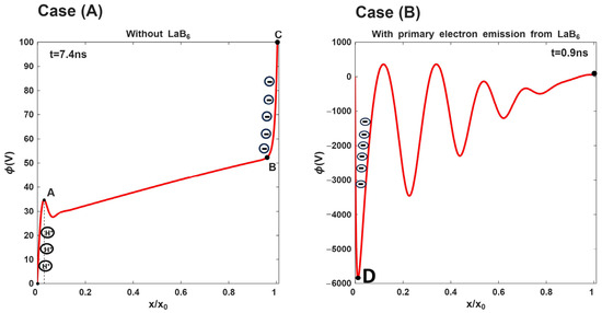
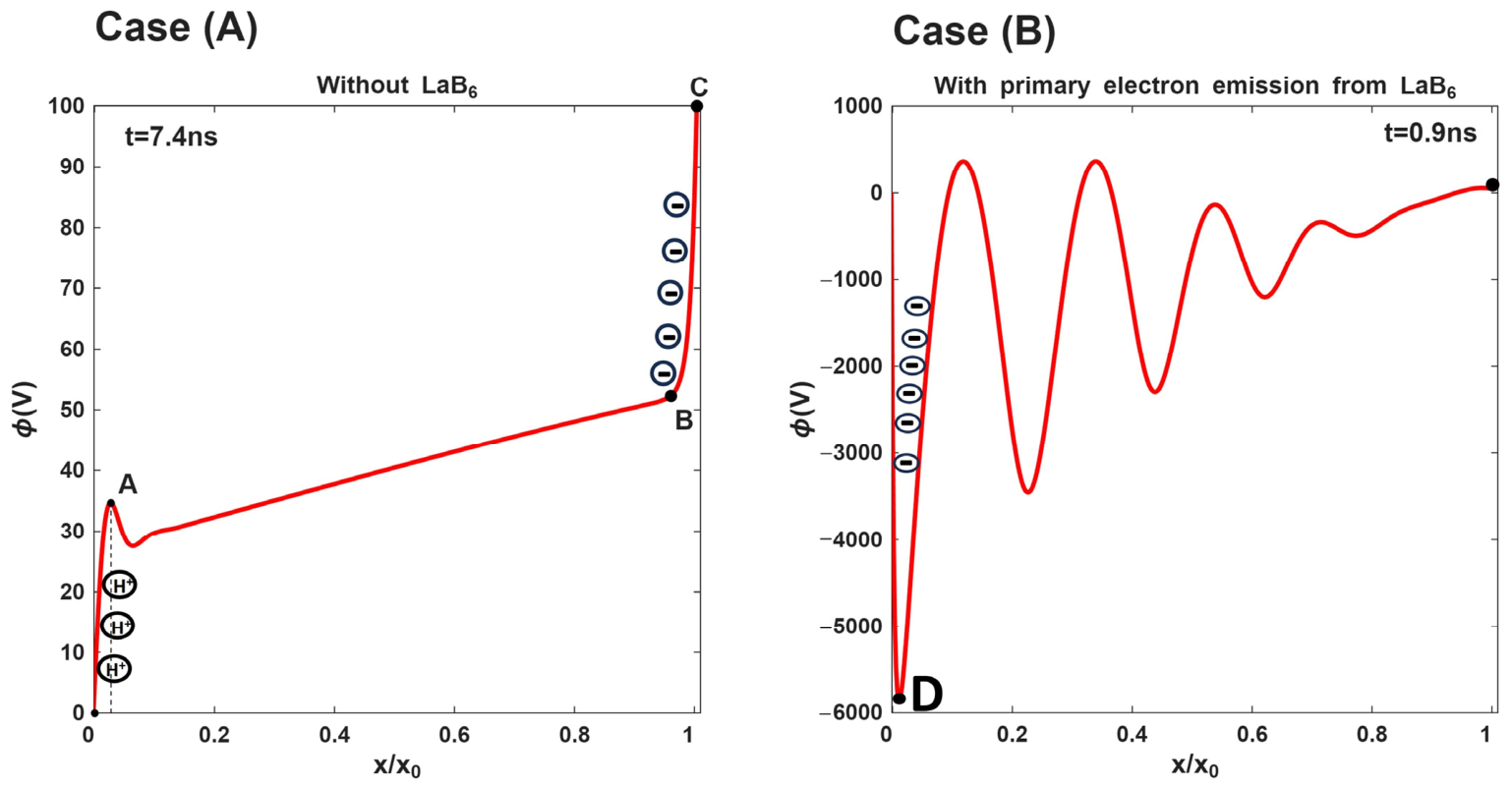
Figure 3A shows a simulation without LaB6 slab in the cathode and a 100 V electric potential is applied across the gas chamber with . For comparison, Figure 3B shows the simulation results with the same parameters as in Figure 3A, but a LaB6 slab is applied in the cathode.
Figure 3.
Case (A), potential profile for simulation without LaB6 slab with applied potential across the cathode and anode, and . The potential drop between points B and C is the positive anode fall, while the potential drop between origin and point A is the cathode fall. In Case (B), the thermionic electrons are emitted from LaB6, and . A potential dip at point D near the LaB6 surface can reach −5800 volts. The electric potential dip of −5800 V near the cathode and the electric potential of 100 V at the anode lead to the acceleration of electrons (ions) toward the anode (cathode), and hence the two-stream instability leads to potential peaks and dips variation with peaks and dips of a few hundred volts.
In Figure 3A, an electric potential is applied across the cathode (. Some electrons in the plasma chamber are attracted by the applied positive potential at to form a potential dip around point B. The lower potential at the cathode tends to attract ions to the left region between and point A. The ion density near is lower than the electron density near B. This may be due to a larger ion mass (lower electron mass) and hence a slower (faster) moving speed.
It is interesting to point out that the electric potential profile is similar to the potential distribution between the cathode and anode in Figure 4 of the review paper by Anders [14]. The potential drop between points B and C is the positive anode fall, while the potential drop between the origin and point A is the negative cathode fall.
Figure 4.
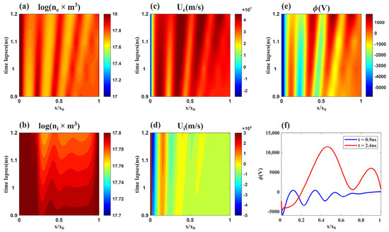
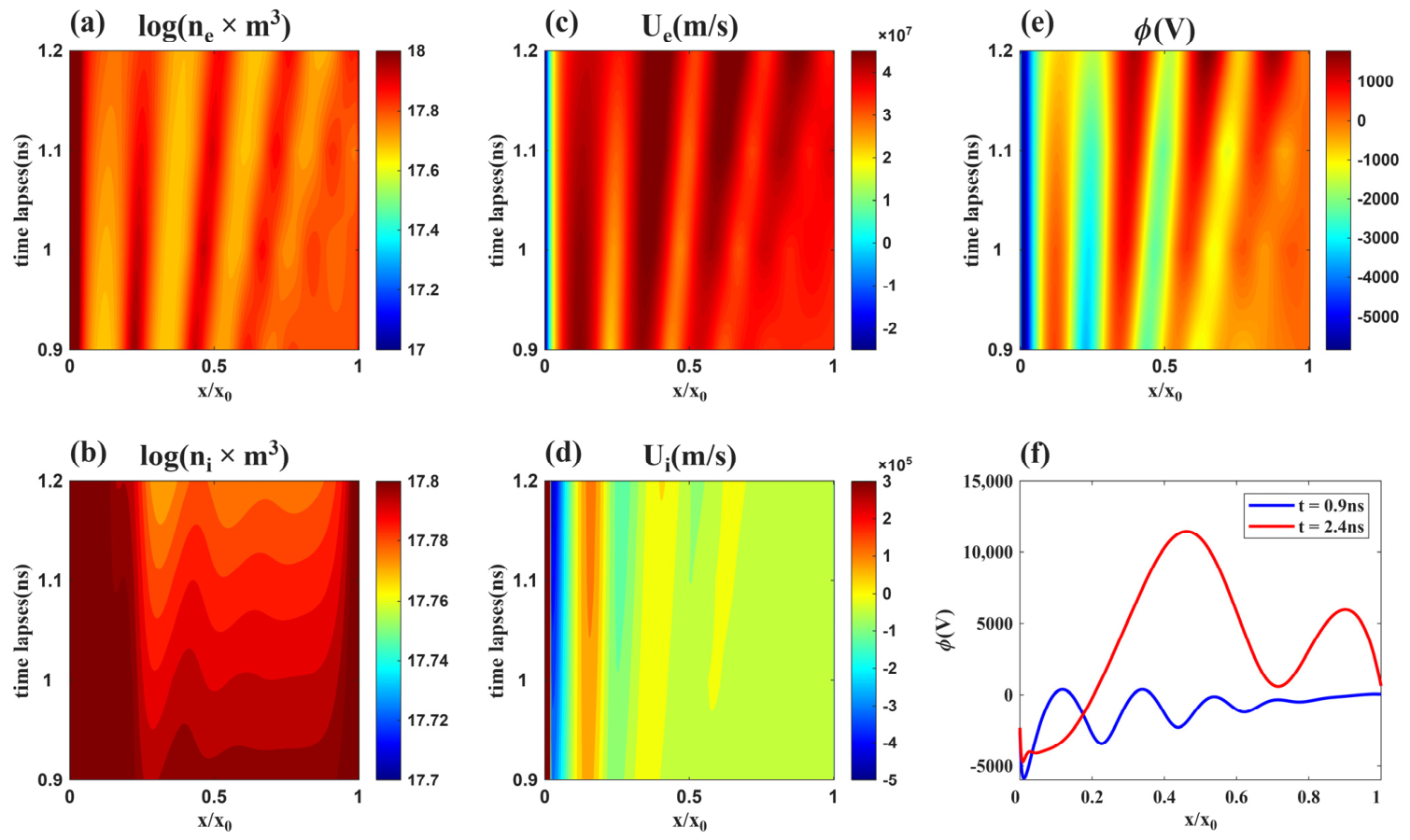
Simulation results of Case B in Figure 3 showing the formation of electrostatic waves due to the two-stream instability. We show the time histories of (a) electron and (b) proton number densities, (c) and (d) velocities, and (e) electric potential as color contours. The time lapses between are shown on the bottom right panel in (f). The electric potential peak reaches the maximum value (~12.0 kV) when t = 2.4 ns.
In Figure 3B, a simulation with a LaB6 slab installed in the cathode and 100 V potential is applied in the 20 mm chamber () between the cathode and the anode. The neutral H2 is filled with , which is equivalent to the density of . The thermionic electrons are emitted from the LaB6 surface and carry a 10 A current. In this case, a potential dip near the LaB6 surface can exceed 1000 volts. In the arc discharge, the two-stream instability occurs and leads to potential peaks of a few hundred volts. The theory of two-stream instability will be developed in the following simulation case.
In the simulation case shown in Figure 4, the density and velocity distributions in the x–t plane show clearly the presence and growth of wavy patterns, which are caused by the electron-ion two-stream instability. This case shows a clear pattern of the electrostatic waves. The potential peak can reach nearly 11.4 kV at , and the dip can reach about −0.6 kV (listed in Case 9 of Table S1). The wavy potential structure may last for a few nanoseconds and quickly fades away. The number of peaks and dips depends on the plasma density and electron velocity. These waves are nearly stationary oscillations in the plasma (electron) frame and can move in the laboratory frame.
The electron-ion two-stream instability can be solved by the linear plasma dispersion relation:
where is the electron plasma frequency, is the proton plasma frequency, and is the wave number [3,27,28,29]. The electron plasma frequency and the proton plasma frequency and ) can be obtained from:
Here, is the wave frequency. The linear dispersion relation is solved based on the electrostatic two-fluid equations for cold and homogeneous plasmas [28]. Note that the plasma frequency is on the order of Hz, about one order of magnitude higher than the electron-neutral collision frequency. Hence, the collision effect can be ignored when solving this dispersion relation.
The electron plasma frequency is estimated from the electron density used in the simulation. For approximately , the electron plasma frequency is approximately rad/s. The electron-neutral collision frequency is estimated from the neutral density, temperature, and electron-neutral collision cross section, as described in Equation (6). With the parameters used in the simulation, is on the order of Hz. Therefore, the statement that the plasma frequency is about one order of magnitude higher than the electron-neutral collision frequency is based on these calculated characteristic frequencies.
As illustrated in Lyu [28], Equation (11) can be replaced as follows:
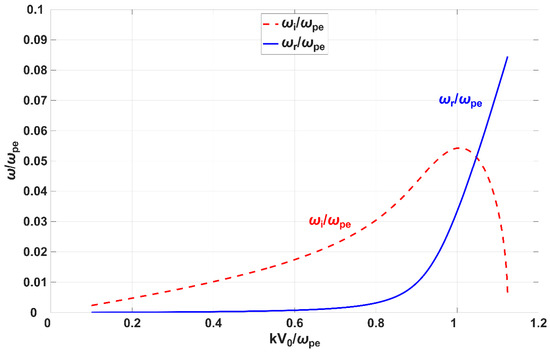
where There are four roots in Equation (14). Only the roots with positive growth rate ( are plotted in Figure 5. As shown in Figure 5, there is a long channel tube, in which the wave structure can be analyzed by the Fourier analysis of and k. The solution of with non-zero wave growth rate gives (a) the wave frequency and (b) the wave number The maximum wave growth rate occurs at and as shown in Figure 5. The corresponding wavelength can be expressed as follows:
Figure 5.
Roots of Equation (14) with only positive growth rate of electron-ion two-stream instability. The real part (blue solid line) and the corresponding growth rate (red dotted line) are plotted as a function of normalized wave number .
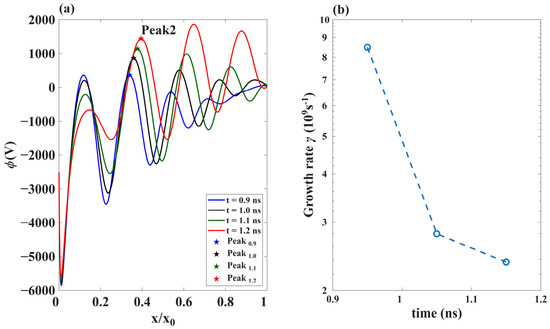
Based on the plasma parameters ( m/s, , and obtain from Equation (12)) and the linear theory, we obtain and the maximum growth rate from (15). For the simulation in Figure 4, there are four potential peaks, and the corresponding wavelength is , close to the theoretical value In Figure 6a, we plot the electric potential as a function of x at different simulation times, t = 0.9, 1.0, …, 1.2 ns. It can be seen that the magnitude of the electric potential peak and dip grows with time t for all four wave peaks and dips.
Figure 6.
(a) The electric potential as a function of x at different simulation times, t = 0.9, 1.0, …, 1.2 ns for Case (B) in Figure 3. There are four wave peaks and four dips. (b) The growth rate of electric potential Peak 2 (denoted by pentagrams) is plotted as a function of time, ranging from .
The growth rate of the electric potential Peak 2 can be calculated from electron density peak values at different times. The growth rate of peaks is plotted as a function of time in Figure 6b. The growth rate of wave Peak 2 ranges from to , which is smaller than the maximum theoretical growth rate. This difference may be caused by the non-uniform profile of and difference between the simulated wavelength and theoretical peak wavelength .
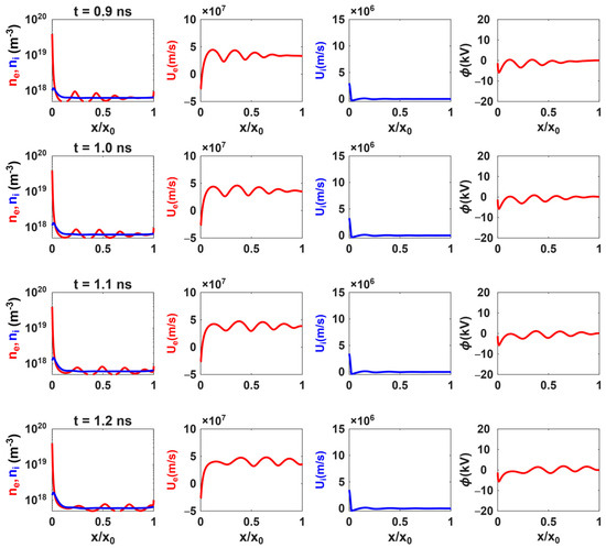
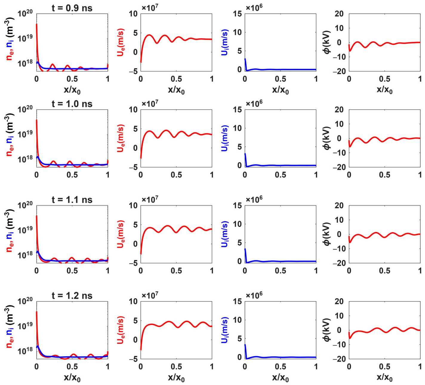
In Figure 7, we show the simulation (Case B in Figure 3B) results at time 0.9, 1.0, 1.1, and 1.2 ns. In this case, an electric potential dip is formed due to the high-density electron layer and the magnitude can reach one kilovolt as shown in the electric potential profiles.
Figure 7.
Simulation results (Case B in Figure 3) of ion (blue) and electron (red) number densities , velocities , and electric potential profiles at time 0.9, 1.0, 1.1 and 1.2 ns. In this case, the boundary electron density near increases to approximately due to continuous electron emission from the LaB6 slab.
Thermionic emitted electrons lead to the formation of an electron layer near the left boundary (). As a result of this electron layer, the electric potential has a sharp decrease from to . The electric potential then increases gradually to volts at the right boundary (anode). The potential difference between and at is large. The average electric field in the chamber is negative (). The negative electric field in the chamber will accelerate electrons to high speed m/s, while ions are accelerated in the left direction with small velocity due to their large mass. The electrons and ions are accelerated in the opposite directions, which can lead to the electron-ion two-stream instability. In the electric potential profile, large amplitude electrostatic waves are formed due to this instability, and the wave amplitude may reach tens of kilovolts. The electron and ion number density and velocity profiles also show similar patterns. The wavy potential structure may last for a few ns.
In Figure 7, the peak electric potential can reach about 2000 V, the electric potential dip can reach −6.0 kV. Note that, in a weakly ionized plasma with temperature 0.5–0.75 eV, an electron can attach to a hydrogen atom H to form a negative hydrogen particle . The density of negative hydrogen () is expected to be small compared with density due to its low production rate [30]. We ignore the contribution from ions in the multi-fluid simulation. The formation of negative electric potential dips (positive electric potential peaks) can accelerate negative hydrogen ions (positive protons) toward the LaB6 slab.
In the multi-fluid theory, unstable normal modes can arise whenever the electron and ion flowing velocities are different [28,29,31]. The total electron flow energy, integrated over the entire tube, decreases during the growth of streaming instability. The growth wave energy arises mainly from the decrease in the electron flow energy within the simulation domain. In this study, we found that the two-fluid plasma electron-ion two-stream instability can be excited. It is the relative velocity between ion flow and electron flow that provides the free energy for the electron-ion two-stream instability.
We estimate the diameter of the arc discharge by comparing a power input of 200 watts for the arc charge with the total kinetic and electric energy in the simulation domain. We calculate the total kinetic energy (electric energy) per area at 1.8 ns of the entire simulation domain and obtain 150 (164 ). The energy provided by the power input at 200 watts over the period of 1.8 ns is . We obtain an upper bound for the diameter of the arc discharge:
Note that the length of the arc discharge is 2 mm, which is 10 times of . Moreover, we also simulate cases of emitted thermionic current as 15 A for three different sets of hydrogen pressure, three sets of applied voltage, and three sets of distances in the next section.
3.3. Comparisons for Simulation Results with Different Parameters
Table S1 lists 48 cases simulated with different sets of parameters, which include the neutral H2 pressure p, the neutral density , the electric potential at the anode, and the system (tube) length . The resulting potential peak and potential dip are also listed in Table S1.
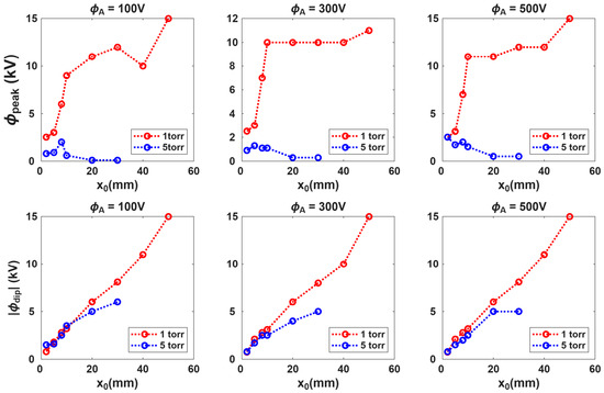
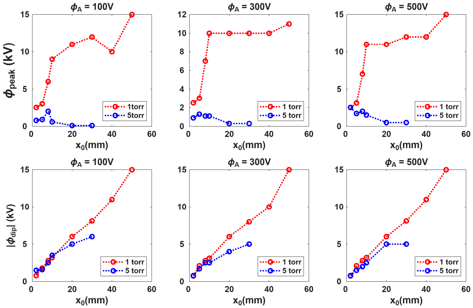
Figure 8 shows the resulting and as a function of (distance between cathode and anode) under applied voltages of 100 V, 300 V, and 500 V from left to right columns. The top (bottom) panels in Figure 8 show the resulting . The red hollow circles are for the cases with 1 torr of neutral hydrogen pressure in the chamber. The black (blue) hollow circles denote the cases with 5 torr (10 torr) of neutral hydrogen (H2) in the chamber. The resulting ranges from 0.1 kV to 45.0 kV, while the resulting ranges from 0.6 kV to 38.0 kV.
Figure 8.
Base on the results of 48 cases in Table S1, the variations are plotted as function as (top panels). The variation as function as (bottom panels). The red hollow circles denote the simulations with 1 torr. The blue hollow circles denote the simulations with 5 torr. For the cases (blue line) with and long chamber (), the plasma density is high and can lead to electron density pile up in the later stage of interrupting the simulation.
Table S1 and Figure 8 show that Case 47 has the largest potential peak . The largest potential dip is in Case 47. In Case 47, . Figure 8 shows that the twenty-four cases with 1 torr have quasi-proportional value of and of with applied voltage .
Regarding the dependence on (distance between cathode and anode), a larger has a larger with the same filling H2 pressure, while the dependence of is mixing. For the cases (blue line) with and long chambers (), the plasma density is high and can lead to electron density pile up and interrupting the simulation.
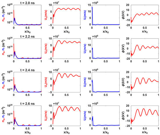
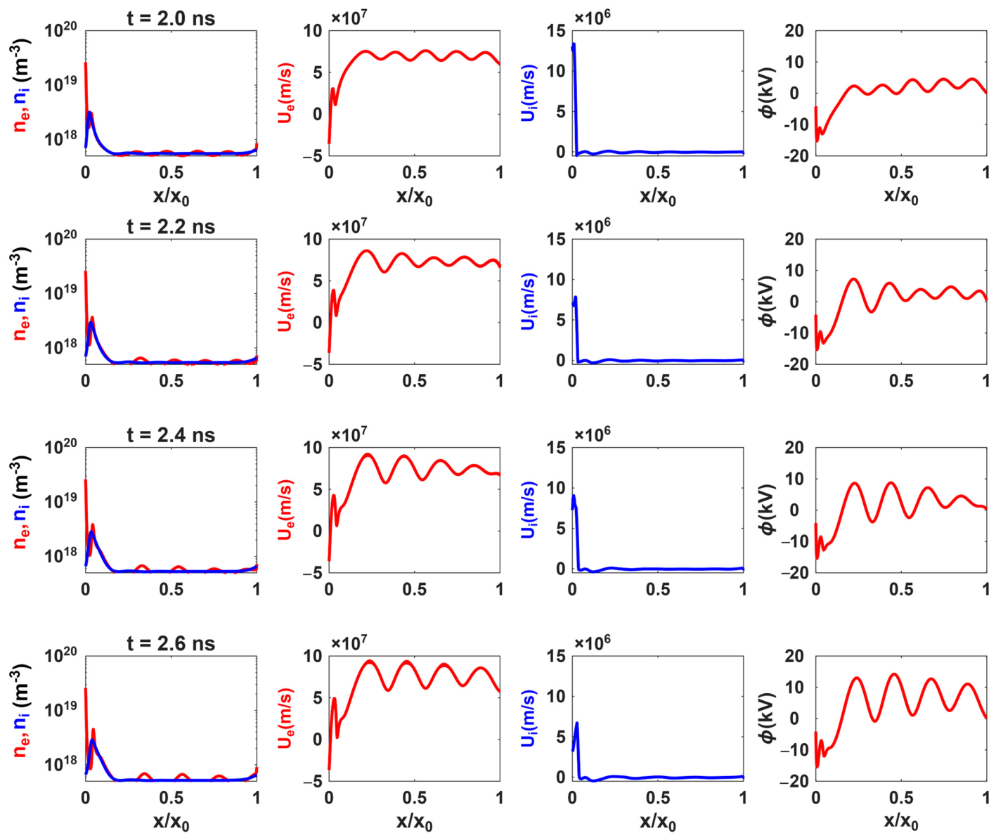
Figure 9 shows the simulation results of Case 47 at 2.0 ns, 2.2 ns, 2.4 ns, and 2.6 ns. In this case, an electric potential dip is formed due to the high-density electron layer and the magnitude can reach −15.0 kV as shown in the electric potential profiles.
Figure 9.
Simulation results (Case 47 in Table S1) of ion and electron number densities , velocities , and electric potential profiles at time 2.0, 2.2, 2.4 and 2.6 ns. In this case, the boundary electron density near increases to approximately due to continuous electron emission from the LaB6 slab. At t = 2.6 ns, and maximum
Thermionic emitted electrons lead to the formation of an electron layer near the left boundary (). As a result of this electron layer, the electric potential has a sharp decrease from to . The electric potential then increases gradually to volts at the right boundary (anode). The average electric field in the chamber is negative (). This negative average electric field in the chamber will accelerate electrons to high speed m/s, while ions are accelerated in the left direction with small velocity due to their large mass. The electrons and ions are accelerated in the opposite directions, which can lead to the electron-ion two-stream instability as discussed earlier. In the electric potential profile, large amplitude electrostatic waves are formed due to this instability, and the wave amplitude may reach tens of kilovolts. The electron and ion number density and velocity profiles also show similar patterns. The wavy potential structure may last for a few ns.
4. Transportation of Protons and Electrons Through High-Density Neutrals (Hydrogen Gas) with Strong Electric Fields
The formation of electron layer leads to a strong electric field, which can accelerate protons. During the acceleration, proton-neutral collisions occur, and a fraction of the protons cannot be accelerated to the peak energy as they reach the LaB6 target. In the following, we consider the proton-neutral collision effect and use the Monte Carlo method to simulate the acceleration and collision process to obtain the energy distributions of protons reaching the LaB6 target for possible nuclear fusion application.
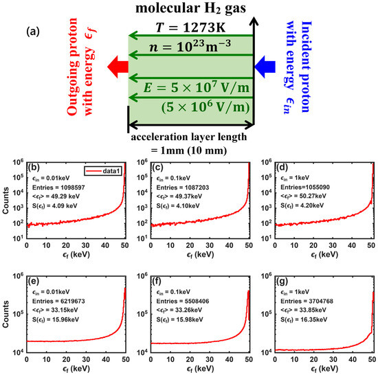
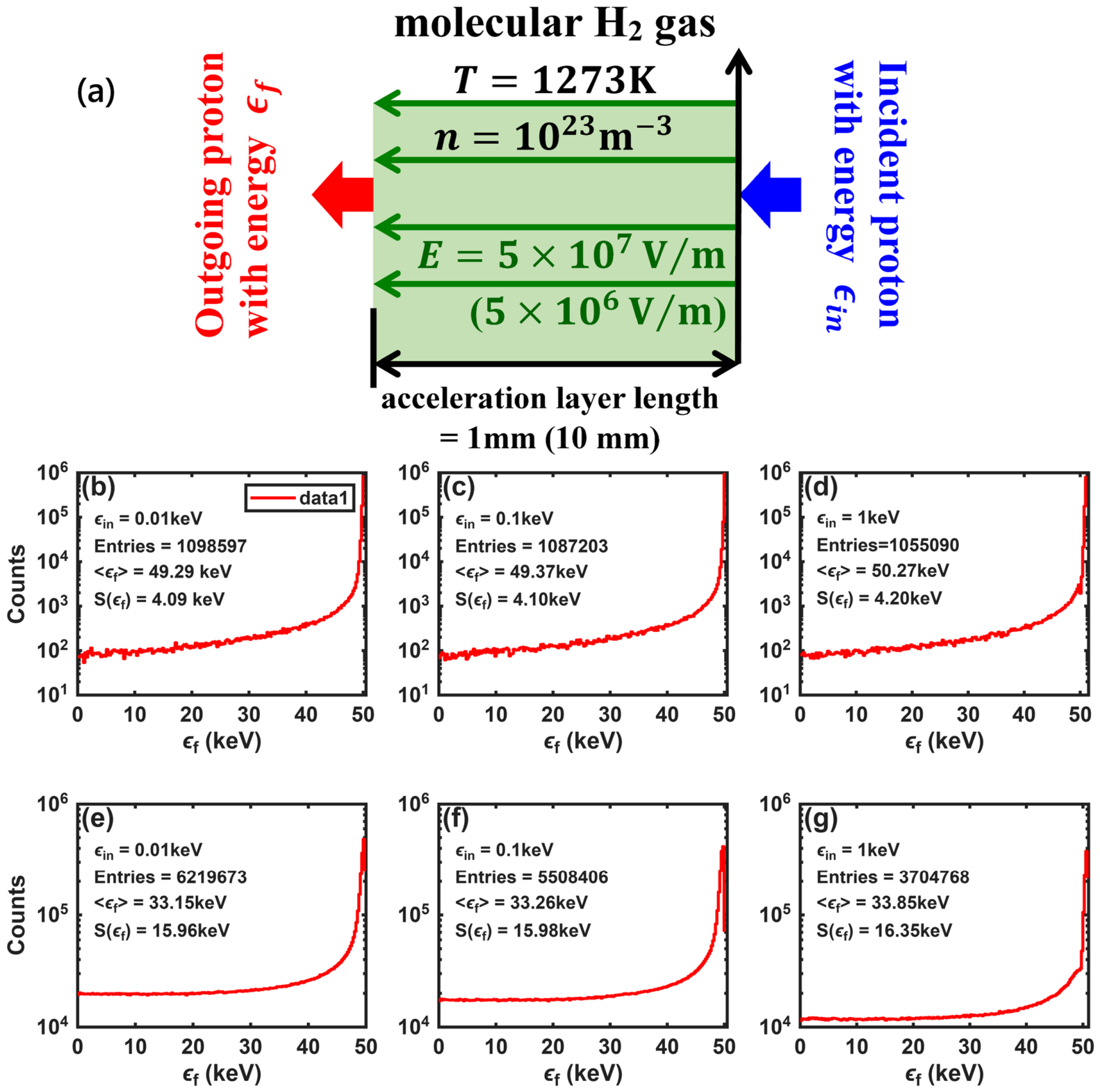
In the following, the proton transportation through the high-density molecular hydrogen with a strong electric field is simulated by Geant4 10.5 (GEometry ANd Tracking) [32,33,34,35], which is a Monte Carlo toolkit used for the simulation of the transportation of particles through matter. For simplicity, we consider that the electric field in the chamber is uniform and constant in the Geant4 simulation. The schematic diagram is illustrated in Figure 10a. The uniform electric field with the strength of 5.0 × 10⁷ V/m (5.0 × 10⁶ V/m) is set with a thickness of 1 mm (10 mm), and the electric potential difference is 50 kV. The results for the cases with a total potential of 10–40 kV are similar to the 50 kV case. High-density neutrals (molecular hydrogen) are uniformly filled in the space. The picture we consider here is that a proton with an initial energy is injected into the hydrogen gas. The proton undergoes acceleration and collisions, and its final energy is recorded as it reaches the other side.
Figure 10.
(a) Schematic diagram of the proton transportation in a molecular gas with density . A uniform electric field is applied across the acceleration layer with length 1 mm (10 mm). The number of entry protons in the Geant4 simulation ranges from 1,055,090 to 6,219,673. (b–f) Energy distribution of outgoing protons for the incident proton with energy 0.01, 0.1, and 1 keV with acceleration layer lengths of (b–d) 1 mm and (e–g) 10 mm. In all cases, the acceleration electric potential across the chamber is 50 kV. The mean value and standard deviation of the outgoing energy are also shown.
Figure 10b–g shows the energy distribution of outgoing protons for different incident energies = 0.01, 0.1, and 1 keV with acceleration layer lengths of 1 and 10 mm. The density of neutral is and the temperature is 1273 K. The number of entry protons for Monte Carlo calculations is . The mean energy and standard deviation of the outgoing energy are also given. One can see that the mean outgoing energy is close to the electric acceleration energy 50 keV. It seems that the electric field acceleration plays a dominant role in the transportation while the energy loss from collisions is small.
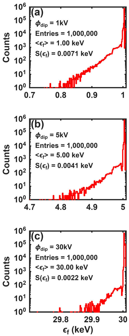
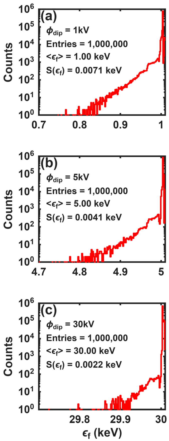
The potential dip ranges from kilovolts to tens of kilovolts and can accelerate electrons. Figure 11 shows the energy distribution of incident electrons with an initial energy 10 eV accelerated by the potential dip 1, 5, and 30 kV with an acceleration layer length of 1 mm. The density of neutral is with a temperature of 1273 K. The number of entry electrons is . The mean energy and standard deviation of the final energy are given. The mean outgoing energy is close to the electric acceleration energy 1, 5, and 30 keV, where is the fundamental charge, Coulomb. The energy loss from collisions is small. The results are not sensitive to the neutral hydrogen () temperature for 1000–1500 K.
Figure 11.
Energy distribution of incident electrons with an initial energy 10 eV accelerated through the potential difference (a) 1 kV, (b) 5 kV, and (c) 30 kV with an acceleration layer length of 1 mm. The location of first is close to the cathode (LaB6). The mean value and standard deviation of the outgoing energy are also shown.
5. A Brief Summary of the Conducting-Channel Model and Application
5.1. A Brief Summary of the Conducting-Channel Model
In this paper, a conducting-channel model is proposed for generating energetic particles in a plasma chamber. The chamber is initially filled with neutral hydrogen gas with density from to , corresponding to 1–5 torr at 300 K for ideal gas conditions. An arc discharge is sustained by an externally applied electric potential across the cathode (slab) and anode, ranging from several hundreds to 1 kV in voltage and several amperes in current, thereby inducing a partially ionized hydrogen plasma within the chamber. As the LaB6 slab heats up, the emitted electrons accumulate to form a layer of negative charge density locally near the cathode.
The multi-fluid simulation conducted in this study shows that the electron layer together with the imposed voltage across the plasma chamber can lead to formation of a large electrostatic potential with dips and peaks of exceeding 10 kilovolts. While our one-dimensional simulation neglects the magnetic field generated by the current flow in the arc discharge and the associated plasma instabilities, it demonstrates that the azimuthal magnetic field associated with the current filament exerts minimal effects on particle orbits. The first potential dip is formed due to the presence of the electron layer. The density diffusion and velocity viscosity in the simulation are important to create a large potential dip near (the cathode). As long as the first potential dip near is deep enough, the acceleration of ions (electrons) toward (away from) the cathode due to the large electric potential leads to the electron-ion two-stream instability. The multiple potential peaks and dips can then be formed. Electron fluid and electron particles within the chamber can be accelerated by these potential dips and peaks.
We have also carried out experiments based on the simulation of this paper. The experiment set is reported in [36]. Due to the limitation of the chamber size and to avoid changing the original plasma distributions in the chamber, the measurements of the electron density, the electric voltage of the electrons, and electron temperature are not obtained. The experiment is not completed and only measures the temperature variation of the cooling water flowing inside the flanges and chamber walls. Therefore, we cannot directly compare the difference between the simulation and the experiment.
The findings and insights derived from these simulations will be cross-referenced with experimental data in forthcoming publications, providing a comprehensive analysis of the research outcomes.
5.2. A Possible Application to the Conducting Channel Associated with Lightning
The lightning associated with the negatively (positively) charged cloud is called negative (positive) cloud-to-ground (CG) lightning. The configuration in Figure 1 is very similar to a negatively charged cloud, air, and the conducting Earth [37,38,39]. The electric potential between the charged cloud and the Earth’s ground is typically 250–400 kV [18,40]. A conducting channel is formed before the onset of lightning. The electric potential in the conducting channel associated with some plasma processes in the lightning tube can reach 50–70 MV [41]. The high electric potential along the lightning channel can lead to the presence of run-away electrons and the generation of X-rays and Gamma rays [41]. Our future work may apply the two-stream instability developed in this paper to provide a possible theory for the formulation of the high potential 50–70 MV lightning phenomena in nature.
Supplementary Materials
The following supporting information can be downloaded at: https://www.mdpi.com/article/10.3390/plasma9030023/s1, Table S1 The parameters of 48 simulation cases with the presence of thermionic current of 10A associated with the electron emission from LaB6; Figure S1. A diagram of the azimuthal magnetic field generated by the arc currents in the conducting channel.
Author Contributions
The team leader of the theoretical research project, L.-C.L.; initialization, K.-H.L. and L.-C.L.; participation in the theoretical discussions and the formulation of the simulation code, L.-C.L., K.-H.L. and H.-K.J.; carrying out the multiple-fluid simulations, K.-H.L. and H.-K.J.; using the Geant4 code to obtain the transport of ions and electrons through the dense hydrogen gas and the penetration depth of the layer by energetic protons, D.-D.N.; the final results were obtained in the intense discussions among the four authors; L.-C.L., K.-H.L., H.-K.J. and D.-D.N. contributed to the writing of the paper. All authors have read and agreed to the published version of the manuscript.
Funding
This research was funded by Alpha Ring International Limited.
Data Availability Statement
The data that supports the findings of this study are available within the article.
Acknowledgments
The discussions with David Chu, Peter Hsieh, Fay Li, Paul Chau, Hao Lin Chen, Allan Chen, Alexander Gunn, Cheng-Lin, Kuo, Ted Cremer, and Y. K. Chu are appreciated. Support and encouragement of Peter Liu and A. Y. Wong are gratefully acknowledged.
Conflicts of Interest
Authors Lou-Chuang Lee, Kun-Han Lee and Hau-Kun Jhuang were employed by the company Alpha Ring Asia In-corporation. The remaining authors declare that the research was conducted in the absence of any commercial or financial relationships that could be construed as a potential conflict of interest. The funders had no role in the de-sign of the study; in the collection, analyses, or interpretation of data; in the writing of the manuscript; or in the decision to publish the results.
References
- Hairapetian, G.; Stenzel, R.L. Observation of a stationary, current-free double layer in a plasma. Phys. Rev. Lett. 1990, 65, 175–178. [Google Scholar] [CrossRef] [Scilit] [PubMed]
- Hairapetian, G.; Stenzel, R.L. Particle dynamics and current-free double layers in an expanding, collisionless, two-electron-population plasma. Phys. Fluids B Plasma Phys. 1991, 3, 899–914. [Google Scholar]
- Quon, B.H.; Wong, A.Y. Formation of Potential Double Layers in Plasmas. Phys. Rev. Lett. 1976, 37, 1393–1396. [Google Scholar] [CrossRef] [Scilit]
- Conde, L.; León, L. Multiple double layers in a glow discharge. Phys. Plasmas 1994, 1, 2441–2447. [Google Scholar] [CrossRef] [Scilit]
- Kaganovich, I.D.; Sydorenko, D. Band structure of the growth rate of the two-stream instability of an electron beam propagating in a bounded plasma. Phys. Plasmas 2016, 23, 112116. [Google Scholar] [CrossRef] [Scilit]
- Wittenberg, H.H. Gas Tube Design from Electron Tube Design; RCA Electron Tube Division: Harrison, NJ, USA, 1962; p. 25. [Google Scholar]
- Bogaerts, A.; Neyts, E.; Gijbels, R.; Van der Mullen, J. Gas discharge plasmas and their applications. Spectrochim. Acta Part B At. Spectrosc. 2002, 57, 609–658. [Google Scholar] [CrossRef] [Scilit]
- Lister, G.G.; Lawler, J.E.; Lapatovich, W.P.; Godyak, V.A. The physics of discharge lamps. Rev. Mod. Phys. 2004, 76, 541–598. [Google Scholar] [CrossRef] [Scilit]
- Becerra, M.; Pettersson, J.; Franke, S.; Gortschakow, S. Temperature and pressure profiles of an ablation-controlled arc plasma in air. J. Phys. D Appl. Phys. 2019, 52, 434003. [Google Scholar] [CrossRef] [Scilit]
- Benilov, M.S. Modeling the physics of interaction of high-pressure arcs with their electrodes: Advances and challenges. J. Phys. D Appl. Phys. 2020, 53, 013002. [Google Scholar]
- Cunha, M.D.; Kaufmann, H.T.C.; Santos, D.F.; Benilov, M.S. Simulating changes in shape of thermionic cathodes during operation of high-pressure arc discharges. J. Phys. D Appl. Phys. 2019, 52, 504004. [Google Scholar] [CrossRef] [Scilit]
- Siewert, E.; Baeva, M.; Uhrlandt, D. The electric field and voltage of dc tungsten-inert gas arcs and their role in the bidirectional plasma-electrode interaction. J. Phys. D Appl. Phys. 2019, 52, 324006. [Google Scholar]
- Xue, S.; Boulos, M. Transient heating and evaporation of metallic particles under plasma conditions. J. Phys. D Appl. Phys. 2019, 52, 454002. [Google Scholar] [CrossRef] [Scilit]
- Anders, A. Glows, arcs, ohmic discharges: An electrode-centered review on discharge modes and the transitions between them. Appl. Phys. Rev. 2024, 11, 031310. [Google Scholar] [CrossRef] [Scilit]
- Lee, K.H.; Lee, L.C.; Wong, A.Y. Acceleration of ions and neutrals by a traveling electrostatic wave. Phys. Plasmas 2018, 25, 023113. [Google Scholar] [CrossRef] [Scilit]
- Wong, A.Y.; Shih, C.-C. Enhancement of Nuclear Fusion in Plasma Oscillation Systems. Plasma 2022, 5, 176–183. [Google Scholar] [CrossRef] [Scilit]
- Wong, A.Y.; Lee, K.H.; Lee, L.C. Simulation of dynamics of rotating weakly ionized plasmas. Phys. Plasmas 2024, 31, 013101. [Google Scholar] [CrossRef] [Scilit]
- Harrison, R.G.; Nicoll, K.A.; Mareev, E.; Slyunyaev, N.; Rycroft, M.J. Extensive layer clouds in the global electric circuit: Their effects on vertical charge distribution and storage. Proc. R. Soc. A Math. Phys. Eng. Sci. 2020, 476, 20190758. [Google Scholar] [CrossRef] [Scilit]
- Edels, H.; Gambling, W.A. Excitation Temperature Measurements in Glow and Arc Discharges in Hydrogen. Proc. R. Soc. Lond. Ser. A Math. Phys. Sci. 1959, 249, 225–236. [Google Scholar] [CrossRef] [Scilit]
- Saha, M.N. LIII. Ionization in the solar chromosphere. Lond. Edinb. Dublin Philos. Mag. J. Sci. 1920, 40, 472–488. [Google Scholar] [CrossRef] [Scilit]
- Saha, M.N.; Fowler, A. On a physical theory of stellar spectra. Proc. R. Soc. Lond. Ser. A Contain. Pap. A Math. Phys. Character 1921, 99, 135–153. [Google Scholar] [CrossRef] [Scilit]
- Froula, D.H.; Glenzer, S.H.; Luhmann, N.C., Jr.; Sheffield, J. (Eds.) Chapter 6—Constraints on Scattering Experiments. In Plasma Scattering of Electromagnetic Radiation, 2nd ed.; Academic Press: Boston, MA, USA, 2011; pp. 143–183. [Google Scholar]
- Froula, D.H.; Glenzer, S.H.; Luhmann, N.C., Jr.; Sheffield, J. (Eds.) Chapter 5—Collective Scattering from a Plasma. In Plasma Scattering of Electromagnetic Radiation, 2nd ed.; Academic Press: Boston, MA, USA, 2011; pp. 103–142. [Google Scholar]
- Huba, J.D. NRL Plasma Formulary; Naval Research Laboratory: Washington, DC, USA, 2019.
- Chapman, S.; Cowling, T.G. The Mathematical Theory of Non-Uniform Gases; An Account of the Kinetic Theory of Viscosity, Thermal Conduction and Diffusion in Gases, 3rd ed.; Burnett, D., Ed.; Cambridge University Press: Cambridge, UK, 1970. [Google Scholar]
- Goebel, D.M.; Watkins, R.M. Compact lanthanum hexaboride hollow cathode. Rev. Sci. Instrum. 2010, 81, 083504. [Google Scholar] [CrossRef] [Scilit] [PubMed]
- Arnush, D.; Nishikawa, K.; Fried, B.D.; Kennel, C.F.; Wong, A.Y. Theory of double resonance parametric excitation in plasmas. Phys. Fluids 1973, 16, 2270–2278. [Google Scholar] [CrossRef] [Scilit]
- Lyu, L.-H. Two-Stream Instability. In Elementary Space Plasma Physics; Airiti Press: Taipei, Taiwan, 2014. [Google Scholar]
- Nicholson, D.R. Two-Stream Instability. In Introduction to Plasma Theory; Wiley: Hoboken, NJ, USA, 1983; pp. 166–169. [Google Scholar]
- Prelec, K.; Sluyters, T. Formation of Negative Hydrogen Ions in Direct Extraction Sources. Rev. Sci. Instrum. 1973, 44, 1451–1463. [Google Scholar] [CrossRef] [Scilit]
- Chen, F.F. Two-Stream Instability. In Introduction to Plasma Physics and Controlled Fusioin; Springer International Publishing: Los Angeles, CA, USA, 2015; pp. 198–201. [Google Scholar]
- Agostinelli, S.; Allison, J.; Amako, K.A.; Apostolakis, J.; Araujo, H.; Arce, P.; Asai, M.; Axen, D.; Banerjee, S.; Barrand, G.J.; et al. Geant4—A simulation toolkit. Nucl. Instrum. Methods Phys. Res. Sect. A Accel. Spectrometers Detect. Assoc. Equip. 2003, 506, 250–303. [Google Scholar] [CrossRef] [Scilit]
- Allison, J.; Amako, K.; Apostolakis, J.E.; Araujo, H.A.; Dubois, P.A.; Asai, M.A.; Barrand, G.A.; Capra, R.A.; Chauvie, S.A.; Chytracek, R.A.; et al. Geant4 developments and applications. IEEE Trans. Nucl. Sci. 2006, 53, 270–278. [Google Scholar] [CrossRef] [Scilit]
- Dong, X.; Cooperman, G.; Apostolakis, J. Multithreaded Geant4: Semi-Automatic Transformation into Scalable Thread-Parallel Software; Springer: Berlin/Heidelberg, Germany, 2010. [Google Scholar]
- Allison, J.; Amako, K.; Apostolakis, J.; Arce, P.; Asai, M.; Aso, T.; Bagli, E.; Bagulya, A.; Banerjee, S.; Barrand, G.J.; et al. Recent developments in Geant4. Nucl. Instrum. Methods Phys. Res. Sect. A Accel. Spectrometers Detect. Assoc. Equip. 2016, 835, 186–225. [Google Scholar] [CrossRef] [Scilit]
- Chen, C.-Y.; Chu, D.; Laing, H.-W.; Lin, J.-Y.; Liu, N.-W.; Jhuang, H.-K.; Hsieh, C.-J.; Jheng, M.-C.; Ho, C.-H.; Hsing, R.; et al. Calorimetric evidence for excess heat generation in a proton-boron glow-discharge system. Under Review. Sci. Rep. 2026. [Google Scholar]
- Alanakyan, Y.R. Structure of conducting channel of lightning. Phys. Plasmas 2013, 20, 082106. [Google Scholar] [CrossRef] [Scilit]
- Pasko, V.P. Atmospheric physics: Electric jets. Nature 2003, 423, 927–929. [Google Scholar] [PubMed]
- Su, H.T.; Hsu, R.R.; Chen, A.B.; Wang, Y.C.; Hsiao, W.S.; Lai, W.C.; Lee, L.C.; Sato, M.; Fukunishi, H. Gigantic jets between a thundercloud and the ionosphere. Nature 2003, 423, 974–976. [Google Scholar] [CrossRef] [Scilit] [PubMed]
- Feynman, R.; Leighton, R.; Sands, M. The Feynman Lectures on Physics, Vol. II: The New Millennium Edition: Mainly Electromagnetism and Matter; Basic Books: New York, NY, USA, 2011. [Google Scholar]
- Dwyer, J.R.; Uman, M.A. The physics of lightning. Phys. Rep. 2014, 534, 147–241. [Google Scholar] [CrossRef] [Scilit]
Disclaimer/Publisher’s Note: The statements, opinions and data contained in all publications are solely those of the individual author(s) and contributor(s) and not of MDPI and/or the editor(s). MDPI and/or the editor(s) disclaim responsibility for any injury to people or property resulting from any ideas, methods, instructions or products referred to in the content. |
© 2026 by the authors. Licensee MDPI, Basel, Switzerland. This article is an open access article distributed under the terms and conditions of the Creative Commons Attribution (CC BY) license.