Advanced Numerical Methods for a First-Kind Fredholm Integral Equation in Potential Field Continuation

Abstract

In this research, surface Au concentration measurements are considered as a spatially correlated geochemical field associated with deep occurrences of disturbing masses using real geological exploration data from the Novo-Khairuzovsky gold deposit in East Kazakhstan. The approach is based on the relationship between potential-field continuation problems and reconstruction of subsurface geological anomalies from surface observations. The considered approaches include Tikhonov and Lavrentiev regularization, SVD, and TSVD. Special attention is given to regularization parameter selection using the L-curve method, Morozov discrepancy principle, and GCV. Comparative computational analysis is performed to evaluate the accuracy, stability, and efficiency of these methods in solving first-kind Fredholm integral equations. Results are assessed using error metrics and spatial visualization of reconstructed fields within a Geographic Information System (ArcGIS), enabling consistent geospatial interpretation. Results show that Lavrentiev regularization with L-curve criterion provides the most stable and reliable reconstruction across all depths, achieving high correlations ($R=0.8876$ at 100 m and $R=0.8049$ at 200 m) with low reconstruction errors. Tikhonov regularization performs acceptably at 100 m but becomes less stable at greater depths. Among spectral methods, TSVD improves stability compared with classical SVD, while standard SVD shows weak correlations and larger reconstruction errors due to high noise sensitivity.

1. Introduction

There are many mathematical and geophysical methods for predicting mineral deposits in the bowels of the Earth based on the analysis of gravitational, magnetic, seismic and geochemical data. Numerical methods, methods for solving inverse problems, as well as modern machine learning and artificial intelligence technologies are widely used to improve the accuracy of forecasting [1,2,3].

One of the key tasks of gravimetric and magnetic exploration is to continue potential fields in the direction of sources of disturbances. The process of extending the potential to the region of occurrence of disturbing masses plays an important role in the interpretation of anomalies, in particular in the framework of parametric selection methods. This approach is particularly effective when identifying individual geological features in complex vertically layered environments. In some cases, the limiting depth $H$, to which a stable continuation of a potential function is possible, can serve as an informative characteristic of the depth of occurrence of disturbing sources [4,5,6,7].

It should be noted that the task of extending potential fields belongs to the class of ill-posed problems in the sense of Jacques Hadamard [8,9]. This means that small errors in the initial data can lead to significant deviations of the approximate solution from the exact one at any depth level $z$. Given that the initial information is formed on the basis of geophysical or geochemical measurements, which inevitably contain experimental errors, this property significantly complicates the task of numerical interpretation.

In the mathematical formulation, the problem of extending potential functions, as a rule, is reduced to solving the Fredholm integral equation of the first kind, which confirms its ill-posed nature and requires the use of special methods and numerical analysis.

In the review paper [10], the key areas of modern research are systematized, including methods of regularization, wavelet analysis and iterative approaches, as well as an analysis of the existence and convergence of solutions. The fundamental aspects of the theory of ill-posed and inverse problems are described in detail in [11,12,13,14], which substantiates the need for an integrated approach combining rigorous theoretical analysis with effective numerical methods, and emphasizes the importance of an adequate choice of basic functions to ensure stability and accuracy of the solution.

Regularization methods occupy a central place in solving integral equations of the first kind. The classical Tikhonov approach is used to stabilize solutions after discretization of the problem [15,16], as well as in combination with other numerical methods. The Lavrentiev method is considered as an alternative that allows obtaining closed-form solutions for some classes of problems [17]. Modern research is aimed at developing nonlinear and adaptive regularization methods [18,19,20,21], including their application to nonlinear and noisy problems. In [22], an improved regularization method was proposed that takes into account the structure of the problem and ensures high stability and accuracy, while in [23,24] extensions of classical approaches to fuzzy and discrete models are considered.

Among the approximation methods, considerable attention is paid to methods based on singular value decomposition. In [25,26], SVD is used to analyze and stabilize solutions, and truncating small singular values reduces the effect of noise. Randomized SVD algorithms have been proposed for high-dimensional problems [27,28], which significantly reduce computational costs while maintaining accuracy.

The analysis of the works shows that modern methods for solving Fredholm integral equations of the first kind are developing towards a combination of regularization, spectral methods and efficient sampling algorithms.

In this research, surface Au concentration measurements are considered as a spatially correlated geochemical field associated with deep occurrences of disturbing masses. The corresponding mathematical formulation is described by a two-dimensional Fredholm integral equation of the first kind with a Poisson-type kernel. The Poisson-type kernel performs the function of a continuation and smoothing operator, providing analysis of the spatial structure of anomalies and reconstruction of deep distributions [29].

The approach is based on the relationship between potential-field continuation problems and reconstruction of spatially distributed subsurface geological anomalies from surface observations. The developed model represents a computational inversion framework for reconstructing the deep structure of anomalous zones [30,31].

The study is based on real gold exploration data from the Novo-Khairuzovsky site in East Kazakhstan at depths of 100 m and 200 m, which makes it possible to investigate the stability of the reconstruction procedure under noisy geological data conditions.

The effectiveness of various numerical methods for approximating the two-dimensional problem of extending potential fields based on real geological data was studied, including Tikhonov regularization method, Lavrentiev regularization method, as well as singular value decomposition (SVD) and its truncated modification (TSVD). To determine the optimal value of the regularization parameter in the Tikhonov and Lavrentiev methods, various selection strategies are considered, in particular, the L-curve method, the Morozov residual principle, and the generalized cross-validation (GCV) method.

A computational comparison of these approaches is carried out in order to evaluate their accuracy, stability, and computational efficiency in the numerical solution of the integral equation.

The novelty of the present work can be summarized as follows:

The study is focused on the reconstruction of deep anomalous distributions using real gold exploration data from the Novo-Khairuzovsky site in East Kazakhstan. All numerical experiments, comparative analyses, and reconstruction procedures are performed on real noisy geological exploration data obtained at depths of 100 m and 200 m.

Within a unified computational framework, Tikhonov regularization, Lavrentiev regularization, singular value decomposition (SVD), and truncated singular value decomposition (TSVD) are implemented and compared under identical conditions on real field measurements. Different parameter choice strategies, including the L-curve method, the Morozov discrepancy principle, and generalized cross-validation (GCV), are also systematically analyzed using the same real geochemical dataset.

An additional numerical experiment on sequential reconstruction from 100 m to 200 m is presented to investigate the accumulation and propagation of errors in multistage continuation procedures for ill-posed inverse problems under realistic geological conditions.

The proposed computational approach is integrated with GIS-based spatial analysis and visualization tools using ArcGIS Pro 3.5 (Esri, Redlands, CA, USA). Integration with ArcGIS enables processing of geological exploration data, construction of two-dimensional maps of anomalous distributions, and expands the capabilities of spatial interpretation, visual analysis, and practical applicability of the obtained reconstruction results.

2. Materials and Methods

2.1. Problem Formulation

In the gravitational field continuation problem for flat two-dimensional anomalies, the potential satisfying the Laplace equation in the region $z>-H$ is determined from known surface data (z is vertical axis, and $H$ is depth). Using the integral representation of the solution makes it possible to reduce the Dirichlet boundary value problem to the Fredholm integral equation of the first kind with respect to an unknown potential distribution at depth. The resulting problem of extending the field in the range $-H<z<0$ is ill-posed, since the solution is highly sensitive to errors in the initial data [7].

In the present study, the approach is based on the relationship between potential-field continuation problems and the reconstruction of spatially distributed subsurface geological anomalies from surface observations [30,31]. This mathematical framework is adapted for reconstructing deep anomalous distributions from surface measurements of gold (Au) concentration. The corresponding model is formulated as a two-dimensional Fredholm integral equation of the first kind: [4,7]:

$$\left(Aq\right)\left(x,y\right)={\iint }_{\Omega }K(x,y,s,t)q(s,t)dsdt=u\left(x,y\right),$$

(1)

where $K\left(x,y,s,t\right)\in L_2\left({\mathsf{\Omega }}^2\right)$ is a real and symmetric kernel, $q(s,t)\in L_2\left(\mathsf{\Omega }\right)$ is the desired concentration distribution in the deep region $z>0$, $u(x,y)\in L_2\left(\mathsf{\Omega }\right)$ is a surface information function measured values on the surface $z=0$, $H$ is a depth of the source, $\mathsf{\Omega }=\left(\right(a,b)\times (a,b\left)\right)\subset {\mathbb{R}}^2$ is a limited area of integration.

The research uses a two-dimensional Poisson kernel for a half-space of the form

$$K(x,y,s,t)={\displaystyle \frac{1}{2\pi }}{\displaystyle \frac{H}{{\left((x-s{)}^2+(y-t{)}^2+H^2\right)}^{3/2}}},$$

(2)

where $\left|H\right|>0$ is the depth of the productive horizon. This kernel describes the smoothing of the signal as it is transferred from depth to surface and corresponds to the fundamental solution of the problem of continuing the harmonic function at $z<H$.

In fact, on the surface of $z=0$, some approximation of $u_{\delta }(s,t)$ to the function $u(s,t)$ is known. Accordingly [6], there are many functions $q(s,t)$ satisfying Equation (1) within a given accuracy

$${\iint }_{\Omega }{\left[\left(Aq\right)\left(x,y\right)-u_{\delta }\left(s,t\right)\right]}^{2}dsdt\le {\delta }^2,$$

among them, there are functions that differ arbitrarily from $\overline{q}(s,t)$—solutions of Equation (1) corresponding to the exact assignment $\overline{u}(s,t)$.

The main requirement for any algorithm for the approximate solution of Equation (1) is that, as $\delta \to 0$, the obtained approximate solution converges to the exact solution of Equation (1).

The choice of the applied numerical methods is determined by the specific properties of the considered inverse problem. The reconstruction of subsurface gold distribution from geochemical measurements is characterized by strong ill-posedness due to the smoothing nature of the Poisson kernel operator, as well as by the presence of noise and measurement uncertainties in real geological data. In this regard, the Tikhonov, Lavrentiev, SVD, and TSVD methods are employed as specialized stabilization approaches that are consistent with the spectral properties of the problem and provide stable and physically meaningful reconstructions of deep anomalies.

2.2. Data Information and Preparation

The research utilized geological data from the Novo-Khairuzovsky site in Southern Altai, including 24,014 samples. Based on the geological data, where a relatively large but non-commercial mineralization zone with low concentrations of Cu, Zn, and Au was identified, cross-sectional and horizontal models of geological parameter distribution were constructed.

Although the spatial coordinates contain $n_x=71$ and $n_y=91$ unique values, the observations do not form a complete Cartesian product. As a result, the expected number of grid nodes is

$$N_{\mathrm{expected}}=n_x\cdot n_y=6461,$$

whereas the actual number of available measurement points is

$$N_{\mathrm{actual}}=6331.$$

This discrepancy arises from the scattered nature of real geophysical observations, missing measurements, and preprocessing steps including the removal of incomplete or unreliable data. Consequently, the dataset represents irregularly distributed (scattered) observations rather than values defined on a structured grid.

All spatial coordinates $\left(x,y\right)$ are given in a rectangular coordinate system and subsequently normalized to the computational domain $\left[\mathrm{0,1}]\times [\mathrm{0,1}\right]$.

The coordinate data and Au (gold) concentration values were scaled for numerical implementation and visualization. The horizontal coordinates have a large range (≈308,000–310,950), and the gold values in the control data are small (≈0.0301–0.0306). Scaling provides convenience for working with matrices and vectors in numerical methods, prevents numerical errors during multiplications and inversions, and simplifies comparison and visual comparison of reconstructed and reference values.

The coordinates are transformed as follows

$$x_s={\displaystyle \frac{x-x_{min}}{x_{max}-x_{min}}}, y_s={\displaystyle \frac{y-y_{min}}{y_{max}-y_{min}}}.$$

After scaling, we have points that lies in the area $\left(x_s, y_s\right)\in \left[\mathrm{0,1}\right]\times \left[\mathrm{0,1}\right]$. The depth is determined as follows:

$$H_s={\displaystyle \frac{H}{L}}, L=\mathrm{m}\mathrm{a}\mathrm{x}(x_{max}-x_{min},y_{max}-y_{min} ).$$

The surface data is defined as

$$u_s={\displaystyle \frac{u(x,y)}{max\left(u\right)}}.$$

After scaling, the integral equation takes the form:

$$u_s\left(x_i,y_i\right)={\iint }_{{\left[\mathrm{0,1}\right]}^2}{\displaystyle \frac{1}{2\pi }}{\displaystyle \frac{H_s}{{\left((x_i-s{)}^2+(y_i-t{)}^2+{H_s}^2\right)}^{\frac{3}{2}}}}q\left(s,t\right)dsdt.$$

(3)

2.3. Discretization of the Integral Model and Numerical Grid Formulation

For the numerical solution of the two-dimensional Fredholm integral equation, the computational domain $\mathsf{\Omega }=\left[\mathrm{0,1}\right]\times \left[\mathrm{0,1}\right]$ is discretized into a uniform grid. Let the grid nodes be defined as

$$x_i=i\Delta x,y_j=j\Delta y,$$

where $i=1,\dots ,N$ and $j=1,\dots ,M$, and

$$\Delta x={\displaystyle \frac{1}{n_x}}, \Delta y={\displaystyle \frac{1}{n_y}}, \Delta S=\Delta x\Delta y,$$

where $n_x,n_y$ are the numbers of subdivisions of the domain $\mathsf{\Omega }$.

The considered two-dimensional Fredholm integral equation of the first kind is approximated numerically using the rectangular quadrature rule (Riemann sum approximation). This allows the transformation of the continuous integral operator into a discrete summation form:

$$u_i\approx {\displaystyle {\sum }_{j=1}^N}{\displaystyle \frac{1}{2\pi }}{\displaystyle \frac{H_s}{{\left((x_i-x_j{)}^2+(y_i-y_j{)}^2+{H_s}^2\right)}^{3/2}}}{q}_j\Delta S,$$

where $N_H=n_x\cdot n_y$ denotes the total number of nodes at a given depth level $H$ and $\Delta S=\Delta x\cdot \Delta y$ is the effective area element in the normalized coordinate system.

It should be emphasized that the number of available observation points is depth-dependent due to the structure of the real geochemical dataset: $N_H=6331$ for the surface dataset (0 m), $N_H=6037$ for the 100 m dataset, $N_H=5392$ for the 200 m dataset.

This notation is introduced to emphasize that each depth level corresponds to a distinct discrete realization of the same spatial sampling process.

The discretization leads to the following linear system:

$$K_H{q}_H=u_H,$$

where $K_H\in {\mathbb{R}}^{N_H\times N_H}$ is the discretized integral operator at depth $H$, $q_H\in {\mathbb{R}}^{N_H}$ is the unknown subsurface distribution, and $u_H\in {\mathbb{R}}^{N_H}$ is the measured surface or depth-dependent data vector.

This formulation naturally reflects the structure of the original physical problem while avoiding artificial interpolation or grid reconstruction, which is particularly important for preserving the integrity of irregular geophysical observations.

The elements of the matrix $K_H$ are defined as

$$K_{ij}^{\left(H\right)}={\displaystyle \frac{1}{2\pi }}{\displaystyle \frac{H_s}{{\left((x_i-x_j{)}^2+(y_i-y_j{)}^2+{H_s}^2\right)}^{3/2}}}\Delta S.$$

(4)

Thus, the original continuous inverse problem is reduced to a discrete ill-posed linear system of the first kind, which forms the basis for applying regularization and spectral stabilization methods in the subsequent sections. For each depth level $H$, two discrete point sets are introduced

$${\mathcal{D}}_H^m=\{x_i^m{\}}_{i=1}^{N_H^m},x_i^m\in {\mathbb{R}}^2, {\mathcal{D}}_H^r=\{x_j^r{\}}_{j=1}^N,x_j^r\in {\mathbb{R}}^2,$$

where ${\mathcal{D}}_H^m$ denotes the measurement locations and ${\mathcal{D}}_H^r$ represents the reconstruction grid nodes.

2.4. Data Comparison and KDTree-Based Matching

To evaluate the accuracy of the reconstructed solution obtained from the discrete system $Kq=u$, a consistent and reproducible mapping between values computed on the regular grid and experimental measurements defined at irregular locations is required. In general, the measured data form a set of points ${\mathcal{D}}_H^m=\{x_i^m{\}}_{i=1}^{N_H^m}$, where $x_i^m\in {\mathbb{R}}^2$, while the reconstructed solution is defined on the uniform computational grid ${\mathcal{D}}_H^r=\{x_j^r{\}}_{j=1}^N$, where $N=n_x\cdot n_y$. Since the measurement locations generally do not coincide with grid nodes, a mapping between these two sets must be established.

The comparison is formulated as a nearest-neighbor problem in the Euclidean space. For each measurement point $x_i^m$, the index of the closest grid node $x_j^r$ is determined by minimizing the Euclidean distance

$$j^{\ast }(i)=arg\underset{j\in \{1,\dots ,N\}}{min}\parallel x_i^m-x_j^r{\parallel }_2.$$

The reconstructed value at the measurement location is then defined as $\widehat{u}\left(x_i^m\right)=q_{j^{\ast }\left(i\right)}.$ This procedure establishes a mapping from irregular measurement locations to the discrete computational grid, enabling direct comparison between observed and reconstructed fields.

A direct implementation of this approach requires computation of all pairwise distances between measurement points and grid nodes, resulting in a computational complexity of $\mathcal{O}(N_H^m\cdot N)$.

For large-scale discretizations, this becomes computationally inefficient, particularly in geospatial inverse problems involving high-resolution grids.

To overcome this limitation, a KDTree (k-dimensional tree) data structure is employed, constructed on the set of grid nodes ${\mathcal{D}}_H^r$. The KDTree is a hierarchical partitioning structure of the space ${\mathbb{R}}^2$, obtained by recursive subdivision along coordinate axes using median-based splitting. Each node of the tree corresponds to a bounded region $R_k\subset {\mathbb{R}}^2$ containing a subset of points.

Nearest-neighbor search in the KDTree (Pittsburgh, PA, USA) is based on a pruning strategy that eliminates regions that cannot contain a point closer than the current best candidate. Specifically, a region $R_k$ is discarded if

$$d(x_i^m,R_k)>d_{min},$$

and

$$d(x_i^m,R_k)=\underset{x\in R_k}{min}\parallel x_i^m-x{\parallel }_2,$$

where $d_{min}$ denotes the current best (smallest) distance found during the search. If this condition is satisfied, the region $R_k$ is excluded from further exploration, significantly reducing the number of distance evaluations.

Due to this hierarchical structure, the average computational complexity of nearest-neighbor search is reduced to $\mathcal{O}\left(logN\right)$, leading to an overall complexity of $\mathcal{O}(N_H^m·logN)$ for the full matching procedure.

Formally, the KDTree construction is based on recursive partitioning of the point set along alternating coordinate axes ($x$ and $y$) using median splitting, which ensures a balanced tree structure. The nearest-neighbor search proceeds by descending the tree to an initial candidate and then performing backtracking steps to verify whether other branches may contain closer points, based on the distance criterion.

In this study, no interpolation between grid nodes is applied. The reconstructed value at each measurement location is assigned strictly from the nearest grid node, i.e.,

$$\widehat{u}\left(x_i^m\right)=q_{j^{\ast }\left(i\right)}.$$

This ensures a deterministic and fully reproducible comparison procedure, eliminating additional approximation errors introduced by interpolation schemes.

Thus, the KDTree provides an efficient and robust mechanism for metric matching between a structured computational grid and irregular measurement data, enabling stable and reproducible evaluation of reconstructed and observed fields in the inverse problem framework [32].

After performing the KDTree nearest-neighbor matching procedure with a prescribed spatial tolerance criterion, the final numbers of matched points used for quantitative reconstruction assessment were: 5930 points for the surface to 100 m reconstruction experiment; 5310 points for the surface to 200 m reconstruction experiment; 5392 points for the sequential 100 to 200 m reconstruction experiment.

The reduction in the number of matched points relative to the original observation counts is caused by the irregular spatial distribution of real geochemical measurements and the exclusion of points that did not satisfy the prescribed spatial consistency criterion. Consequently, the error and correlation analyses were performed only for spatially consistent matched observations.

2.5. Quantitative Analysis of KDTree-Based Matching Distances

To quantitatively assess the geometric accuracy of the correspondence between measurement locations and nodes of the computational grid, the Euclidean distances induced by the nearest-neighbor matching procedure based on the KDTree structure were additionally analyzed.

For each measurement point $x_i^m$, the Euclidean distance to its nearest grid node was computed as

$$d_i=\parallel x_i^m-x_{j^{\ast }\left(i\right)}^r{\parallel }_2,$$

where $x_{j^{\ast }\left(i\right)}^r$ denotes the closest node in the reconstruction grid.

Based on these distances, statistical measures were evaluated, including the mean distance $\overline{d}$, the maximum distance $d_{max}$, and the standard deviation ${\sigma }_d$.

The computed statistical values are summarized as follows:

For reconstruction from surface to 100 m

$${\overline{d}}_{100}=5.38\times {10}^{-4},{ d}_{max}^{100}=8.78\times {10}^{-2},{ \sigma }_{100}=4.74\times {10}^{-3}.$$

For reconstruction from surface to 200 m

$${\overline{d}}_{200}=4.81\times {10}^{-4},{ d}_{max}^{200}=7.02\times {10}^{-2},{ \sigma }_{200}=4.40\times {10}^{-3}.$$

For sequential reconstruction from 100 m to 200 m

$${\overline{d}}_{100-200}=0.0,{ d}_{max}^{100-200}=0.0,{ \sigma }_{100-200}=0.0.$$

In all cases, the obtained distances remain significantly smaller than the characteristic spatial discretization step of the computational grid $\mathrm{h}$, i.e.,

$$\overline{d},d_{max}\ll h.$$

This confirms that the geometric discrepancy introduced by replacing irregular measurement locations with their nearest grid nodes is negligible compared to the reconstruction error.

Therefore, the KDTree-based nearest-neighbor matching provides not only computational efficiency but also preserves the metric consistency of the comparison procedure between measured and reconstructed fields.

The threshold value used for spatial consistency filtering was applied solely as a preprocessing step to exclude geometrically inconsistent matches and does not affect the computation of KDTree-based distance statistics.

2.6. Lavrentiev’s Regularization Method

After discretization of the two-dimensional integral model, we obtain the system

$$Kq=u^{\delta },$$

where $K$ is the matrix of the discrete operator, $q$ is the vector of the desired depth distribution, and $u^{\delta }$ is the vector of noisy data.

Lavrentiev’s method is based on solving a regularized system [17]

$$(K+\alpha I)q_{\alpha }=u^{\delta },$$

(5)

where $\alpha >0$ is the regularization parameter. The $\alpha$ parameter controls the trade-off between the stability of the solution and the accuracy of matching with the data.

In practical applications, the Lavrentiev regularization method is widely used for stabilizing ill-posed inverse problems arising in geophysical and geochemical modeling, particularly in problems related to potential field continuation and subsurface reconstruction. One of the main advantages of the method is the direct stabilization of the operator through the regularization parameter $\alpha$, which reduces the amplification of noise and computational errors without requiring explicit construction of normal equations.

In the present study, the Lavrentiev method is especially suitable because the discretized Poisson kernel operator is strongly smoothing and leads to a rapid decay of singular values, making the direct inversion procedure unstable even for small perturbations in the measured data. The regularization scheme improves the conditioning of the problem and provides stable approximations of the deep distribution of gold concentration.

From a computational perspective, the method is effective for processing large geochemical datasets and ensures stable reconstruction of subsurface anomalies while preserving the main spatial features of the mineralization distribution.

2.7. Choosing the Optimal Regularization Parameter $\alpha$

Since the resulting system is strongly ill-posed, regularization techniques are required to obtain stable solutions. In this work, both Tikhonov and Lavrentiev regularization methods are employed. The corresponding regularized solutions depend on a parameter $\alpha$, which controls the balance between data fidelity and stability.

To ensure consistency and robustness of the numerical experiments, the regularization parameter was searched over the logarithmically distributed interval

$$\alpha \in [{10}^{-6},{10}^1],$$

using 60 logarithmically spaced candidate values. The same search interval and discretization strategy were applied consistently for all regularization methods and all depth levels to ensure comparability of the obtained results.

Three independent strategies were applied for parameter selection: the L-curve method, generalized cross-validation (GCV), and the Morozov discrepancy principle. This combination allows assessment of solution stability under different assumptions regarding the noise structure and spectral properties of the discretized operator.

If regularization parameter $\alpha$ is too small, the solution becomes unstable and highly sensitive to noise, whereas excessively large values lead to over-smoothing and loss of important information. Therefore, choosing an optimal regularization parameter is a critical step in solving ill-posed inverse problems.

An ill-posed problem is being considered

$$Aq=u^{\delta },$$

where $u^{\delta }$ is the noisy observational data. The application of the Lavrentiev regularization method leads to the equation

$$(A+\alpha I)q_{\alpha }=u^{\delta },q_{\alpha }=(A+\alpha I{)}^{-1}{u}^{\delta }.$$

(6)

Residual functionals and solution norms are introduced [6]:

$$\rho \left(\alpha \right)=‖A{q}_{\alpha }-u^{\delta }‖, \eta \left(\alpha \right)=‖q_{\alpha }‖.$$

(7)

2.7.1. The L-Curve Method

The L-curve method is based on a geometric analysis of the compromise between the norm of the solution and the magnitude of the discrepancy [33]. For a set of values of the parameter $\alpha$, regularized solutions are calculated, after which a parametric curve is constructed in logarithmic coordinates:

$$x\left(\alpha \right)=\mathrm{l}\mathrm{o}\mathrm{g}\rho \left(\alpha \right)=\mathrm{l}\mathrm{o}\mathrm{g}‖A{q}_{\alpha }-u^{\delta }‖,$$

$$y\left(\alpha \right)=\mathrm{l}\mathrm{o}\mathrm{g}\eta \left(\alpha \right)=\mathrm{l}\mathrm{o}\mathrm{g}‖q_{\alpha }‖.$$

The optimal parameter value is selected at the point of maximum curvature of the parametric curve: Numerical experiments show that such a curve usually has a characteristic shape resembling the letter $L$. The range of small values of $\alpha$ corresponds to a small discrepancy and a large solution norm, which indicates overfitting and amplification of the noise component. The region of large values of $\alpha$ is characterized by a strong smoothing of the solution and an increase in the discrepancy

$$\kappa (\alpha )={\displaystyle \frac{\mid x^{\prime }\left(\alpha \right)y^{″}\left(\alpha \right)-y^{\prime }\left(\alpha \right)x^{″}\left(\alpha \right)\mid }{{\left(x^{\prime }(\alpha {)}^2+y^{\prime }(\alpha {)}^2\right)}^{3/2}}}.$$

(8)

The selection criterion has the form:

$${\alpha }_{\ast }=\arg \underset{\alpha }{\max \kappa \left(\alpha \right)},$$

where $\alpha$ is the regularization parameter controlling the balance between solution stability and approximation accuracy, and ${\alpha }_{\ast }$ denotes the optimal regularization parameter corresponding to the maximum curvature of the L-curve.

2.7.2. The Morozov Discrepancy Principle

The Morozov discrepancy principle is a theoretically rigorous method for selecting the regularization parameter [34,35]. It assumes that there is an a priori estimate of the noise level in the data. If the following condition is met

$$‖u^{\delta }-u‖\le \delta ,$$

there is no reason to fit the model to the data with an accuracy higher than the noise level. Here $u^{\delta }$ denotes the observed noisy data, $u$ represents the exact data, and $\delta$ is the noise level.

The regularization parameter is selected from the condition

$$\parallel A{q}_{\alpha }-u^{\delta }\parallel =\tau \delta , \tau \ge 1,$$

where $\tau$ is the discrepancy coefficient controlling the admissible deviation between the residual norm and the noise level.

The equivalent entry is presented as

$$\rho \left(\alpha \right)=‖A(A+\alpha I{)}^{-1}{u}^{\delta }-u^{\delta }‖=\tau \delta ,$$

when the smoothness conditions of the exact solution are met, it is proved that when the noise level tends to zero, the regularized solution converges to the exact one. The asymptotic rule of order for smoothness of degree $p$ has the form:

$$\alpha \sim {\delta }^{{\displaystyle \frac{1}{p+1}}},$$

when the smoothness conditions of the exact solution are met, it is proved that when the noise level tends to zero, the regularized solution converges to the exact one.

2.7.3. Generalized Cross-Validation Method

The generalized cross-validation (GCV) method is based on statistical estimation theory and is used to minimize prediction error. It evaluates the quality of the solution without explicitly splitting the data into training and validation sets, making it effective for inverse and ill-posed problems [36].

When using this method, a regularizing operator is introduced

$$R_{\alpha }=(A+\alpha I{)}^{-1}{, q}_{\alpha }=R_{\alpha }{u}^{\delta },$$

and the resolving operator is represented as

$$H_{\alpha }=A{R}_{\alpha }=A(A+\alpha I{)}^{-1}.$$

GCV functionality $G\left(\alpha \right)$ is defined by the expression

$$G\left(\alpha \right)={\displaystyle \frac{\parallel A{q}_{\alpha }-u^{\delta }{\parallel }^2}{{\left(\mathrm{t}\mathrm{r}\mathrm{a}\mathrm{c}\mathrm{e}\left(I-H_{\alpha }\right)\right)}^2}}={\displaystyle \frac{\parallel \left(I-H_{\alpha }\right)u^{\delta }{\parallel }^2}{{\left(\mathrm{t}\mathrm{r}\mathrm{a}\mathrm{c}\mathrm{e}\left(I-H_{\alpha }\right)\right)}^2}}.$$

The optimal parameter value is selected from the condition

$${\alpha }_{\ast }=\mathrm{a}\mathrm{r}\mathrm{g}\underset{\alpha }{\mathrm{m}\mathrm{i}\mathrm{n}}G(\alpha ).$$

The GCV method is fully automated and does not require prior information about the noise level. However, the method may be computationally expensive and can underestimate the regularization parameter in the presence of high noise levels.

2.8. Tikhonov Regularization Method

Tikhonov regularization was applied to stabilize the solution of the ill-conditioned $Kq=u$ system that occurs when restoring the deep distribution of gold concentration [15,16]. The method is to solve a modified system

$$(K^{\mathrm{\top }}K+\alpha I)q_{\alpha }=K^{\mathrm{\top }}u,$$

where $\alpha >0$ is the regularization parameter, $I$ is the identity matrix, and $q_{\alpha }$ is the regularized solution. The choice of $\alpha$ provides a balance between approximation accuracy and suppression of measurement noise.

Analogously to the Lavrentiev regularization method, the regularization parameter for the Tikhonov method was selected using standard parameter-choice strategies, including the L-curve criterion, Morozov discrepancy principle, and generalized cross-validation (GCV). Numerical experiments showed that the optimal parameter depends on data scaling and discretization properties. In the considered experiments, stable reconstructions were obtained for values of $\alpha$ of order ${10}^{-1}$–${10}^0$, with the optimal value approximately equal to $\alpha \approx 0.86$.

To verify the accuracy of the solution, a comparative assessment was performed at a depth of 100 m. Common points between the reconstructed field and the reference data were identified using KDTree matching, and the reconstruction error was computed as the difference between normalized Au values. The results were visualized using two-dimensional maps demonstrating the spatial distribution of reconstructed concentrations and their agreement with real measurements.

Tikhonov regularization effectively stabilizes the inversion process, reduces the influence of noise, and provides physically meaningful reconstructions of mineral concentration distributions [15]. The method is especially effective for integral kernels associated with diffusion and filtration processes, including the Poisson kernel.

2.9. Singular Value Decomposition (SVD) Method

SVD method is based on the singular value decomposition of the discretized matrix $K$ [26,27],

$$K=U\mathsf{\Sigma }{V}^{\mathrm{\top }},$$

where $U\in {\mathbb{R}}^{m\times m}$ и $V\in {\mathbb{R}}^{n\times n}$ are orthonormal matrices, $\mathsf{\Sigma }\in {\mathbb{R}}^{m\times n}$ is a diagonal matrix containing singular values ${\mathsf{\sigma }}_1\ge {\mathsf{\sigma }}_2\ge \dots \ge {\mathsf{\sigma }}_r\ge 0$, $r=rank\left(K\right)$—the rank of the matrix $K$.

The formal solution has the form

$$q={\displaystyle \sum _{i=1}^r}{\displaystyle \frac{u_i^{\mathrm{\top }}u}{{\sigma }_i}}{v}_i,$$

where ${\sigma }_i, i=1,\dots ,r$ are singular values.

2.10. Truncated Singular Value Decomposition (TSVD) Method

Due to the rapid decay of the singular values ${\sigma }_i$, the components corresponding to small singular values become highly sensitive to noise and computational errors. Therefore, along with the classical SVD approach, the truncated singular value decomposition (TSVD) method is also considered to improve the stability of the obtained solution [28]

$$q_k={\displaystyle \sum _{i=1}^k}{\displaystyle \frac{u_i^{\mathrm{\top }}u}{{\sigma }_i}}{v}_i, k<r.$$

Here, the truncation parameter $k$ plays the role of a regularization parameter, controlling the trade-off between stability and approximation accuracy.

TSVD method is well suited for the considered inverse problem of geological data continuation, since the measured data contain noise and the corresponding matrix $K$ is severely ill-conditioned due to the rapid decay of singular values. In such cases, the classical SVD solution becomes unstable, while TSVD improves stability by truncating small singular components associated with noise amplification. In addition, the truncation parameter $k$ provides control over the degree of regularization, allowing a balance between reconstruction accuracy and stability. By preserving only the dominant singular components, TSVD retains the main structural features of the spatial distribution of mineralization, which is important for reliable reconstruction of subsurface anomalies.

Energy Criterion for Choosing the Parameter $k$

The truncation parameter $k$ in the TSVD method is selected using a 99% cumulative energy criterion, ensuring that the dominant part of the singular-value spectrum is preserved.

The key task in applying the truncated singular value decomposition (TSVD) is the selection of the truncation parameter $k$, which determines the number of singular components retained in the solution. An inappropriate choice of $k$ may lead either to loss of relevant information (for small $k$) or to amplification of noise (for large $k$).

To address this issue, an energy-based criterion is employed, defined through the cumulative contribution of the singular values

$$\mathrm{E}\left(k\right)={\displaystyle \frac{{\sum }_{i=1}^k{\mathsf{\sigma }}_i^2}{{\sum }_{i=1}^r{\mathsf{\sigma }}_i^2}}.$$

Here, $E\left(k\right)$ represents the fraction of the total spectral energy of the operator matrix $K$ captured by the first $k$ singular values, where ${\sigma }_i$ are the singular values and $r$ is the full rank of the system. The optimal truncation level is selected such that a prescribed energy threshold is satisfied, i.e.,

$$E\left(k\right)\ge 0.99.$$

This ensures that the dominant spectral content of the system is preserved while suppressing components associated with small singular values, which are typically dominated by noise.

To further justify the robustness of this selection strategy, a sensitivity analysis with respect to the truncation parameter $k$ was performed. Reconstructions were computed for small, intermediate, and large values of $k$, including the value determined by the energy criterion. The results demonstrate that small values of $k$ lead to excessive smoothing and loss of local anomalies, whereas large values of $k$ amplify the influence of small singular values, resulting in increased noise in the reconstructed solution. In contrast, the value of $k$ selected via the energy criterion provides a stable compromise between noise suppression and preservation of the essential structural features of the reconstructed field.

3. Results and Discussion

3.1. Numerical Experiments and Validation of Reconstruction Methods

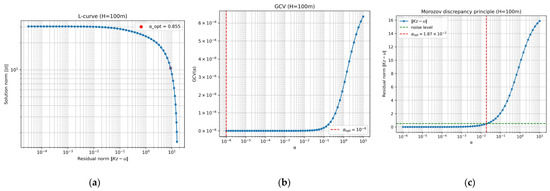
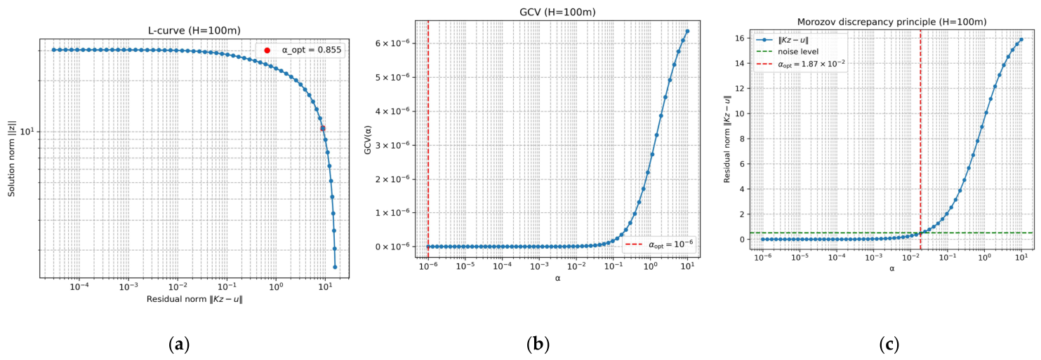
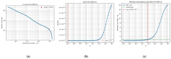
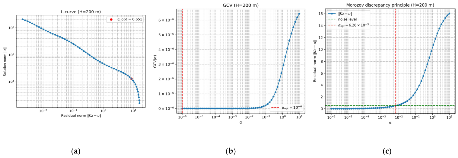
To ensure stable and accurate reconstruction, the regularization parameters for the depth levels of 100 m and 200 m were determined using several parameter selection strategies, including the L-curve criterion, generalized cross-validation (GCV), and the Morozov discrepancy principle (Figure 1a–c and Figure 2a–c). The obtained estimates were subsequently used in the implementation of the Tikhonov and Lavrentiev regularization methods. Comparative analysis demonstrated that the parameters selected by the L-curve method provided the most stable reconstructions for both considered depth levels and were therefore chosen as optimal for the numerical experiments.

Figure 1. Choosing the optimal regularizing parameter (100 m): (a) L-curve method; (b) GCV method; (c) Morozov discrepancy principle.

Figure 2. Choosing the optimal regularizing parameter (200 m): (a) L-curve method; (b) GCV method; (c) Morozov discrepancy principle.

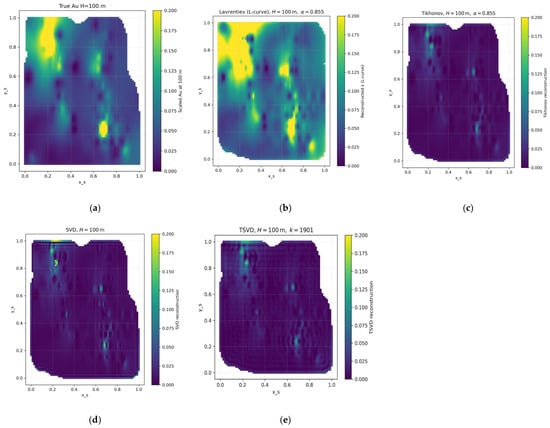
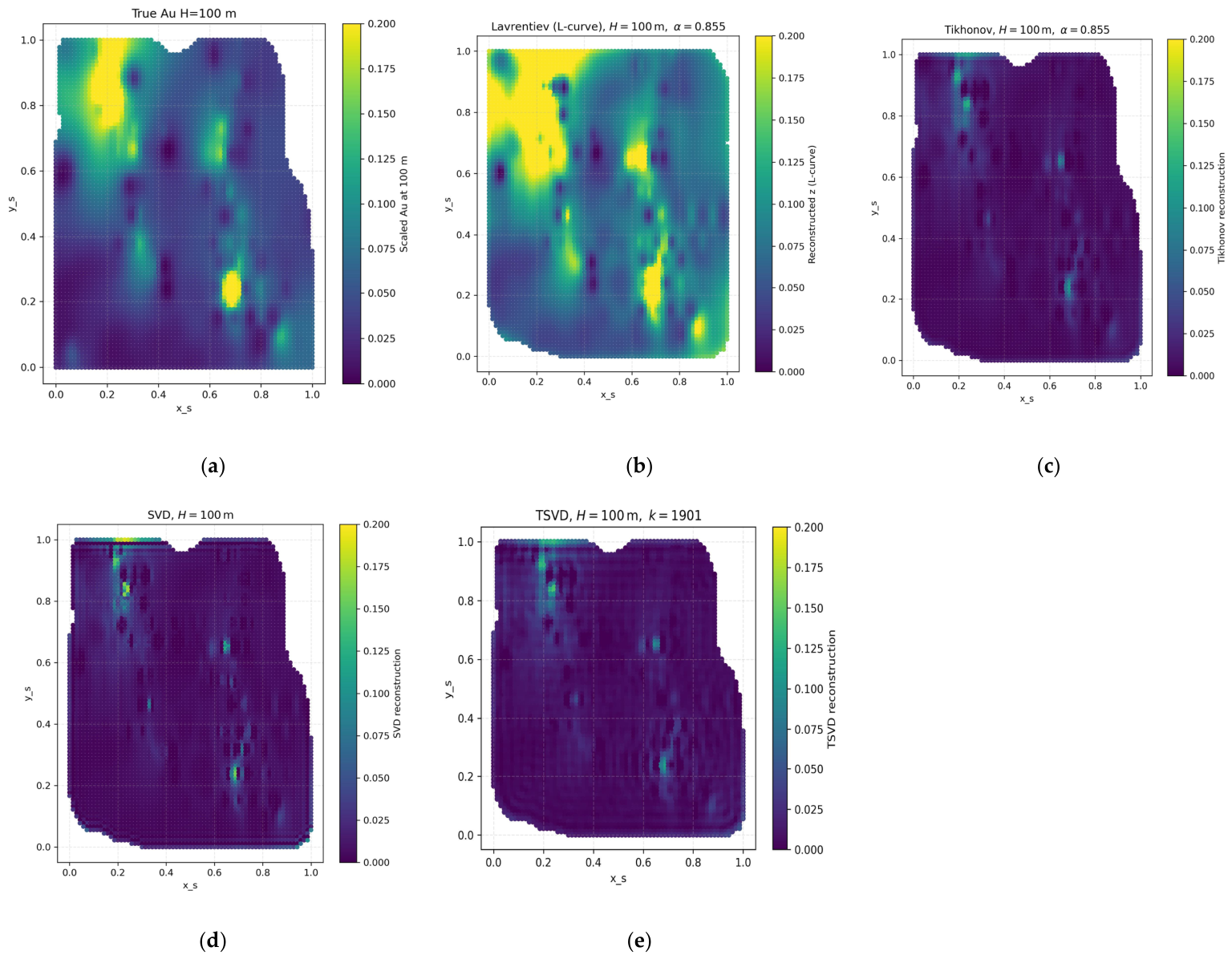
The reconstruction of gold concentration at a depth of 100 m was performed using the Lavrentiev, Tikhonov, SVD, and TSVD methods, and the obtained results were compared with the available real measurement data at the corresponding depth level (Figure 3a–e).

Figure 3. Gold concentration reconstruction at 100 m depth and comparison with measured data: (a) Real measured data at a depth of 100 m; (b) Reconstruction using the Lavrentiev method; (c) Reconstruction using the Tikhonov method; (d) Reconstruction using the SVD method; (e) Reconstruction using the TSVD method.

The results in Table 1 show that at a depth of 100 m, Lavrentiev with L-curve provides the best accuracy, achieving the lowest MAE (0.0428) and RMSE (0.0582), as well as the highest correlation (R = 0.8876). Tikhonov and TSVD demonstrate similar error levels (MAE ≈ 0.0517 and 0.0516), but Tikhonov yields higher correlation than SVD, indicating better spatial consistency. SVD shows the weakest correlation (R = 0.5982), despite comparable error magnitudes. In terms of computational cost, SVD and TSVD are the fastest (0.000762 and 0.001999), while regularization-based methods are slightly more expensive. Overall, Lavrentiev (L-curve) provides the most balanced performance in terms of accuracy and spatial reliability at this depth.

Table 1. Quantitative comparison of reconstruction methods at the 100 m level.

Method	MAE	RMSE	Relative L2 Error	Max Absolute Error	Correlation R	Execution Time
Lavrentiev (L-curve)	0.042818	0.058156	0.672758	0.467702	0.8876	0.687356
Lavrentiev (GCV)	0.179331	0.317727	3.675500	3.549315	0.5983	0.712175
Lavrentiev (Morozov)	0.153566	0.250372	2.896327	2.540127	0.7259	0.720994
Tikhonov (L-curve)	0.051652	0.073145	0.846151	0.896006	0.772638	0.003000
SVD	0.051739	0.073584	0.851225	0.842670	0.598247	0.000762
TSVD	0.051623	0.073191	0.846680	0.888198	0.709220	0.001999

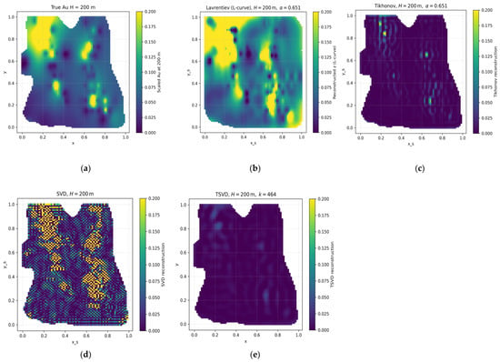
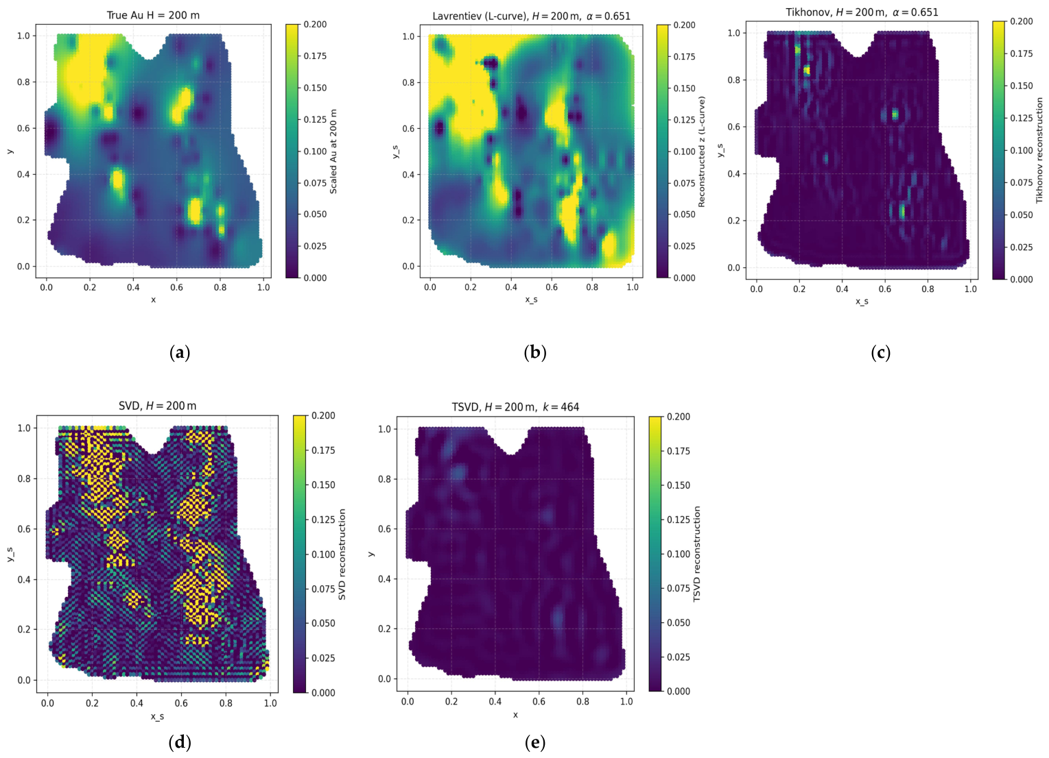
The reconstruction of the gold distribution at a depth of 200 m was performed similarly to the 100 m case using the Lavrentiev, Tikhonov, SVD, and TSVD methods (Figure 4a–e). The availability of measured data at the corresponding depth made it possible to directly compare the reconstructed distributions with real observations and evaluate the accuracy and stability of the applied approaches. The obtained results indicate that reconstruction at greater depths becomes more challenging due to the increasing ill-posedness of the inverse problem and stronger amplification of errors and noise. Therefore, appropriate selection of the regularization parameter plays a crucial role in ensuring stable and accurate reconstruction results.

Figure 4. Gold concentration reconstruction at 200 m depth and comparison with measured data: (a) Real measured data at a depth of 200 m; (b) Reconstruction using the Lavrentiev method; (c) Reconstruction using the Tikhonov method; (d) Reconstruction using the SVD method; (e) Reconstruction using the TSVD method.

Table 2 shows that at a depth of 200 m, the results indicate a clear degradation in performance for several methods. Lavrentiev with L-curve remains the most accurate and stable approach, achieving the lowest errors (MAE = 0.0507, RMSE = 0.0848) and the highest correlation (R = 0.8049). In contrast, Lavrentiev with GCV and Morozov exhibits strong instability with extremely large errors and very low correlation (R = 0.0117 and R = 0.2626), indicating poor parameter selection in the ill-posed regime. Tikhonov and TSVD show moderate performance, with TSVD yielding better correlation (R = 0.5170) than Tikhonov (R = 0.1938), while SVD remains the least stable method (R = 0.0077). In terms of computational cost, SVD and TSVD are the fastest (0.001393 and 0.001610), whereas regularization-based methods are slightly more expensive. Overall, Lavrentiev (L-curve) provides the most reliable performance at this depth.

Table 2. Quantitative comparison of reconstruction methods at the 200 m level.

Method	MAE	RMSE	Relative L2 Error	Max Absolute Error	Correlation R	Execution Time
Lavrentiev (L-curve)	0.050729	0.084846	0.771803	0.723308	0.8049	0.670695
Lavrentiev (GCV)	8.749765	28.313830	257.555954	771.838944	0.0117	0.703176
Lavrentiev (Morozov)	0.411020	0.993349	9.035975	12.810308	0.2626	0.681862
Tikhonov	0.080034	0.106958	0.972940	1.017832	0.193844	0.001711
SVD	0.202807	0.558635	5.081604	13.514551	0.007732	0.001393
TSVD	0.079863	0.105854	0.962894	0.973888	0.517006	0.001610

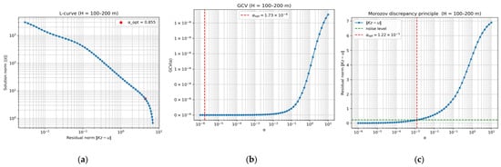
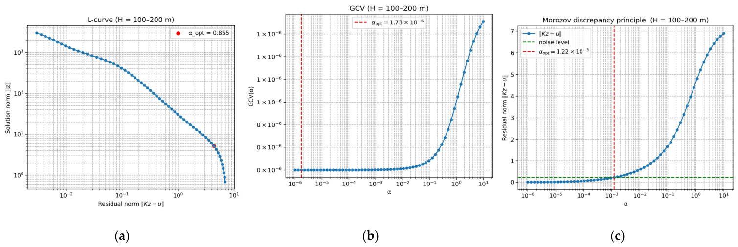
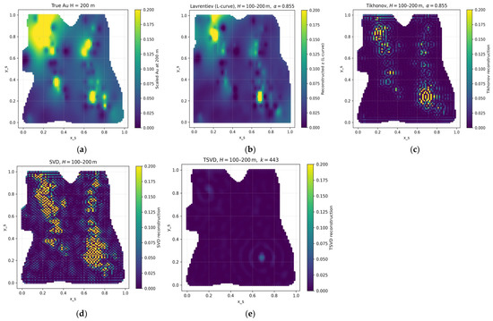
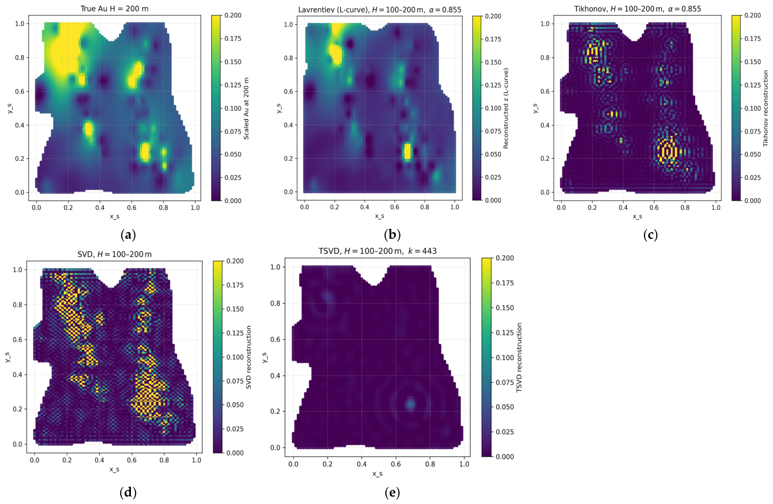
As an additional experiment, sequential depth reconstruction was considered. In this case, data at the level of 100 m were used as input (surface) observations, and the depth parameter in the Poisson kernel was assumed to be $H=100$ m. Thus, the gold distribution was restored at a depth of 200 m.

The obtained results were compared with direct measurements at 200 m, as well as with the reconstruction performed directly from the initial surface data (from 0 m to 200 m). Such a comparison makes it possible to assess the stability of the methods during the sequential transfer of information deep, as well as to identify the possible accumulation of errors during multistep recovery (Figure 5a–c and Figure 6a–e).

Figure 5. Choosing the optimal regularizing parameter (sequential depth reconstruction from 100 m to 200 m): (a) L-curve method; (b) GCV method; (c) Morozov discrepancy principle.

Figure 6. Reconstruction of gold mineralization at 200 m depth based on 100 m depth measurements: (a) Real measured data at a depth of 200 m; (b) Reconstruction using the Lavrentiev method; (c) Reconstruction using the Tikhonov method; (d) Reconstruction using the SVD method; (e) Reconstruction using the TSVD method.

The results presented in Table 3 confirm that the inverse problem becomes increasingly ill-posed over the combined 100–200 m interval. Lavrentiev regularization with the L-curve criterion demonstrates the best overall performance, achieving the lowest errors (MAE = 0.0381, RMSE = 0.0538) and the highest correlation (R = 0.8511), indicating high stability and robustness under depth continuation. In contrast, Tikhonov regularization shows limited performance, with MAE = 0.0962, RMSE = 0.2109, and a very low correlation (R = 0.0373), suggesting a loss of spatial consistency despite numerical stability. The classical SVD method exhibits strong instability, with high reconstruction errors (MAE = 0.1881, RMSE = 0.8763) and an extremely low correlation (R = 0.0080), confirming its sensitivity to noise amplification in ill-posed sequential reconstruction. TSVD improves stability compared to SVD, achieving MAE = 0.0808, RMSE = 0.1069, and R = 0.4916, but remains less accurate than regularization-based methods. In terms of computational cost, SVD and TSVD are the fastest (0.001002 and 0.001001), while regularization-based methods are slightly more expensive. Overall, Lavrentiev (L-curve) clearly outperforms all other approaches in terms of accuracy, correlation, and stability in sequential reconstruction.

Table 3. Quantitative comparison of reconstruction methods for the 100–200 m interval.

Method	MAE	RMSE	Relative L2 Error	Max Absolute Error	Correlation R	Execution Time
Lavrentiev (L-curve)	0.038117	0.053762	0.492434	0.487148	0.8511	0.593778
Lavrentiev (GCV)	5.619334	33.855920	310.104306	1284.780974	0.0163	0.656647
Lavrentiev (Morozov)	0.431252	2.457549	22.509990	78.423032	0.1449	0.628003
Tikhonov	0.096211	0.210850	1.931284	5.649013	0.037268	0.001995
SVD	0.188090	0.876316	8.026641	26.262669	0.008020	0.001002
TSVD	0.080751	0.106913	0.979271	0.970066	0.491575	0.001001

Table 4 summarizes the optimal regularization parameters obtained for all considered inversion methods at different depth levels. The results show that the L-curve criterion provided relatively stable regularization parameters for both Lavrentiev and Tikhonov methods across all investigated depths. In contrast, the GCV criterion consistently selected extremely small regularization parameters, indicating a tendency toward under-regularization and potential instability of the inverse solution. The Morozov discrepancy principle produced intermediate parameter values that varied significantly with depth, reflecting the sensitivity of the method to noise level estimation. For the TSVD approach, the selected truncation level $k$ decreased substantially for deeper intervals, which indicates increasing ill-posedness of the inverse problem and the necessity of stronger spectral filtering.

Table 4. Summary of the selected regularization parameters for different inversion methods and depth levels.

Depth	Method	Parameter Selection	Optimal Parameter
100 m	Lavrentiev	L-curve	0.855467
	Lavrentiev	GCV	1 × 10−6
	Lavrentiev	Morozov	0.018672
	Tikhonov	L-curve	0.855467
	TSVD	Energy criterion	1901
200 m	Lavrentiev	L-curve	0.650968
	Lavrentiev	GCV	1 × 10−6
	Lavrentiev	Morozov	0.006261
	Tikhonov	L-curve	0.650968
	TSVD	Energy criterion	464
100–200 m	Lavrentiev	L-curve	0.855467
	Lavrentiev	GCV	1.726983 × 10−6
	Lavrentiev	Morozov	0.001215
	Tikhonov	L-curve	0.855467
	TSVD	Energy criterion	443

The conducted numerical experiments demonstrate that the stability and reliability of the obtained results strongly depend on the type of method used and the parameter selection strategy. The differences between the methods become especially pronounced with increasing depth, confirming the inherently ill-posed nature of the inverse problem.

Lavrentiev regularization combined with the L-curve criterion produces relatively stable results across all depths and preserves the structure of the reconstructed field effectively. This indicates its ability to suppress noise while maintaining the dominant signal components. In contrast, the Tikhonov method shows a gradual loss of stability with increasing depth, becoming more sensitive to data perturbations.

The instability observed for the GCV and Morozov-based parameter selection strategies is mainly caused by the strongly ill-posed nature of the discretized inverse problem and the rapid decay of the singular-value spectrum, leading to severe ill-conditioning of the system matrix. Under such conditions, the GCV criterion tends to select excessively small regularization parameters, resulting in under-regularization, noise amplification, and unstable reconstructions, especially at larger continuation depths.

For the Morozov discrepancy principle, the noise level was estimated heuristically as 3% of the $L_2$ norm of the normalized data, i.e., $\delta =0.03‖u‖$, which is a common assumption in numerical inverse problems.

To ensure fair comparison, the same $L_2$- based normalization procedure was applied to all datasets and all depth levels. Therefore, the observed instability is not related to within the bounded logarithmic interval ${10}^{-6}\le \alpha \le {10}^1$ using 60 discrete values for all parameter-choice strategies.

Among spectral approaches, TSVD improves stability by filtering out small singular values and preserves structural information better than classical SVD. However, its accuracy still becomes limited at greater depths. Classical SVD, on the other hand, is highly sensitive to noise due to the rapid decay of singular values, which leads to unstable reconstructions.

The additional sequential reconstruction experiment reveals the accumulation of errors during step-by-step continuation in depth. This behavior indicates that small perturbations in the initial data propagate into deeper layers, affecting the overall quality of the solution. Therefore, the use of stable regularization strategies is crucial for reliable deep geological interpretation [37,38,39,40].

3.2. Stability and Sensitivity Analysis of the Inverse Problem

3.2.1. Conditioning Analysis

To evaluate the numerical stability of the discretized inverse problem, we computed the condition number of the system matrix $K$. The obtained value

$$cond\left(K\right) \approx 6.6\times {10}^2$$

indicates that the problem is moderately ill-conditioned in the discrete sense. This implies that the inverse problem is sensitive to small perturbations in the input data, which is a characteristic feature of discretized Fredholm integral equations of the first kind.

3.2.2. Singular Value Spectrum

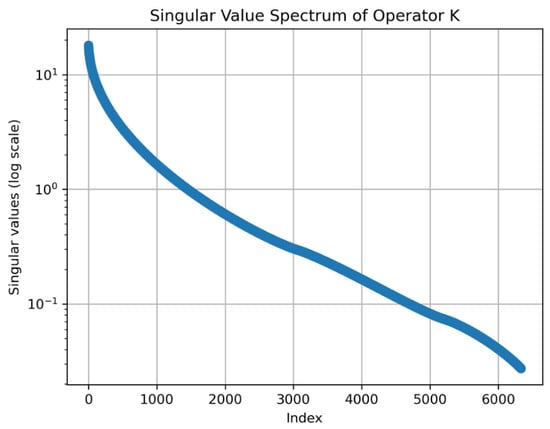
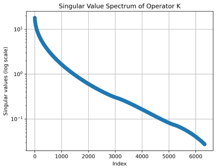
The singular value decomposition of the operator $K$ reveals a smooth and rapid decay of singular values (see Figure 7). Such behavior confirms the ill-posed nature of the inverse problem and indicates strong attenuation of high-frequency components by the forward operator.

Figure 7. Singular value decomposition of the operator $K.$

This spectral decay leads to a loss of information in the small singular value regime, which in turn causes instability in direct inversion and amplifies the effect of noise. These properties justify the necessity of regularization techniques.

3.2.3. $\alpha$

-Sensitivity Analysis

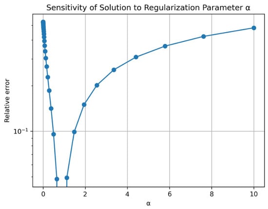
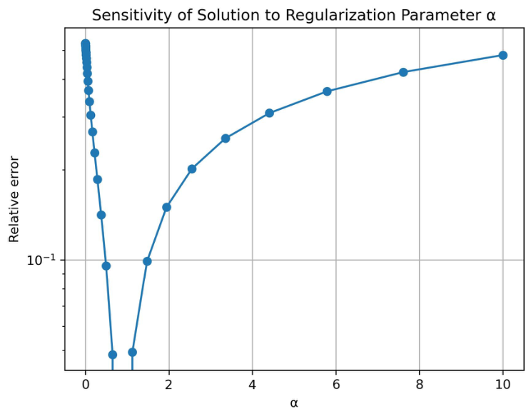
To further investigate the stability of the regularized solution, a sensitivity analysis with respect to the regularization parameter $\alpha$ was performed. The relative error was computed using a reference solution obtained at the optimal L-curve parameter.

The results (Figure 8) demonstrate a highly nonlinear dependence of the reconstruction error on $\alpha$, characterized by a narrow region of optimal regularization. In particular, the error exhibits a sharp minimum, while rapidly increasing for both under-regularization (small $\alpha$) and over-regularization (large $\alpha$).

Figure 8. Sensitivity of solution to regularization parameter $\alpha$

This behavior indicates that the inverse problem is not only ill-posed but also highly sensitive to the choice of regularization parameter. As a result, small deviations from the optimal $\alpha$ lead to significant degradation of the reconstruction quality.

The analysis demonstrates that the instability of regularization parameter selection methods (GCV and Morozov’s discrepancy principle) is driven by the intrinsic ill-posedness of the problem and its high sensitivity to the regularization parameter $\alpha$. The moderately high condition number, rapid decay of singular values, and pronounced α-sensitivity lead to a narrow region of optimal regularization, where even small deviations significantly degrade reconstruction quality. As a result, the GCV method tends to select underestimated values of $\alpha$, leading to under-regularized and noise-amplifying solutions, whereas Morozov’s principle is sensitive to noise level estimation, resulting in unstable parameter selection. Therefore, the observed instability reflects the properties of the underlying ill-posed operator rather than deficiencies of the methods themselves.

3.3. Computational Environment

All numerical computations were performed using Python 3.13.7. The implementation relied on the NumPy 2.2.6, SciPy 1.16.3, Pandas 2.3.3, and Matplotlib 3.10.7 libraries for numerical linear algebra, data processing, and visualization.

The experiments were conducted on a standard desktop workstation with a multi-core CPU. No GPU acceleration was used, and all reported execution times correspond to single-thread CPU computations.

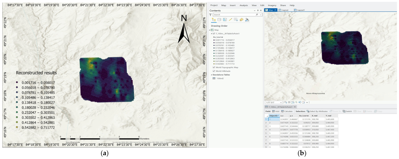
3.4. GIS-Based Spatial Interpretation of Reconstructed Results

To ensure physically meaningful interpretation of the reconstructed subsurface distributions, the numerical results were integrated into a Geographic Information System (ArcGIS Enterprise) as part of the post-processing and spatial analysis pipeline [41].

The discrete reconstructed solutions obtained on the computational grid were exported as georeferenced point datasets, where each grid node was associated with its spatial coordinates and the corresponding estimated gold concentration.

Within the GIS environment, the reconstructed point fields were used to generate continuous spatial representations for different depth levels (100 m and 200 m). This transformation enables a unified spatial comparison of the inversion results obtained by different regularization and spectral methods under identical georeferencing conditions.

The GIS-based representation enables spatial analysis of reconstructed anomalies, localization of high-concentration zones, and comparative evaluation of the stability and physical consistency of the obtained solutions at different depths.

All visualizations were performed within a consistent spatial reference framework, ensuring that comparisons across depth levels and reconstruction methods remain strictly comparable [42].

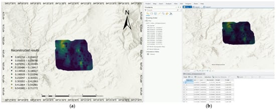
The integration of numerical reconstruction with GIS-based spatial analysis significantly enhances the interpretability, comparability, and geophysical relevance of the obtained results, bridging the gap between mathematical inversion and practical geological decision-making (Figure 9a,b).

Figure 9. GIS-based spatial visualization and interpretation of reconstructed subsurface gold distributions in ArcGIS Enterprise: (a) Reconstructed results using Lavrentiev (L-curve) method; (b) Visualization in ArcGIS Enterprise.

3.5. Validation Protocol and Limitations

The geochemical datasets at depths of 100 m and 200 m, derived from real gold (Au) concentration measurements, were used as reference fields for the quantitative evaluation of reconstruction accuracy. Due to the limited availability of independent in situ subsurface geochemical measurements, a separate external validation dataset was not available in this study.

Therefore, the evaluation procedure is based on an internal consistency validation framework, where the same observational datasets are used in a controlled manner for both parameter selection and reconstruction assessment.

Specifically, the reference fields are partially involved in the parameter selection stage (including the L-curve method, generalized cross-validation (GCV), and the Morozov discrepancy principle), while the reconstruction accuracy is evaluated through direct comparison between reconstructed and observed fields at different depth levels.

To mitigate potential bias associated with the absence of independent test data, multiple regularization parameter selection strategies are employed and cross-compared, including Tikhonov-based approaches and spectral decomposition methods. In addition, validation is performed across multiple spatial configurations (surface-to-100 m, surface-to-200 m, and sequential 100–200 m experiments), which provides a form of cross-scenario consistency check.

Although this approach does not correspond to an external statistical validation in the strict machine learning sense, it is appropriate for deterministic inverse problems, where the primary objective is stable and physically consistent reconstruction of subsurface geochemical fields rather than predictive generalization to unseen data.

4. Conclusions

The article considers the problem of reconstructing the deep distribution of gold concentration from geological measurements within the framework of a two-dimensional integral model with a Poisson-type kernel. The considered inverse problem was reduced to a Fredholm integral equation of the first kind and solved using the Lavrentiev, Tikhonov, SVD, and TSVD methods. In addition, several approaches for selecting the regularization parameter, including the generalized cross-validation (GCV) method, were analyzed.

Numerical experiments were carried out using real geological data from the Novo-Khairuzovsky site in Southern Altai. The research considered surface measurements, as well as data at depths of 100 m and 200 m. Based on the initial data, cross-sectional and horizontal models of gold distribution were constructed on a regular grid. Direct comparisons between reconstructed and measured distributions at different depth levels allowed the reconstruction accuracy and stability of the considered methods to be quantitatively evaluated.

The obtained results demonstrate that the most stable and accurate reconstructions across all considered depths are achieved by Lavrentiev regularization with the L-curve criterion, showing high correlation values at 100 m, at 200 m, and in the sequential reconstruction. Tikhonov regularization provides acceptable accuracy only at shallow depth (100 m); however, a significant decrease in correlation and stability is observed with increasing depth and in sequential reconstruction. Among spectral methods, TSVD yields more stable results compared to classical SVD due to the suppression of small singular values, although it remains less accurate than the Lavrentiev method. Classical SVD is the most sensitive to noise and depth increase, resulting in low correlation values and degraded reconstruction quality.

An additional numerical experiment involving sequential reconstruction from 100 m to 200 m demonstrated the accumulation of reconstruction errors during step-by-step continuation, emphasizing the importance of stable regularization procedures for deep geological interpretation.

The proposed computational methodology can be applied to the analysis of geochemical and geological data for various deposits and geological structures. The developed approach may be useful for the interpretation of subsurface anomalies, forecasting promising mineralization zones, and solving inverse problems arising in mineral exploration and geological modeling.

References

- Aali, A.A.; Shirazy, A.; Shirazi, A.; Pour, A.B.; Hezarkhani, A.; Maghsoudi, A.; Hashim, M.; Khakmardan, S. Fusion of remote sensing, magnetometric, and geological data to identify polymetallic mineral potential zones in Chakchak Region, Yazd, Iran. Remote Sens. 2022, 14, 6018. [Google Scholar] [CrossRef] [Scilit]
- Sun, K.; Chen, Y.; Geng, G.; Lu, Z.; Zhang, W.; Song, Z.; Guan, J.; Zhao, Y.; Zhang, Z. A review of mineral prospectivity mapping using deep learning. Minerals 2024, 14, 1021. [Google Scholar] [CrossRef] [Scilit]
- Ali, A.; Chiang, Y.W.; Santos, R.M. X-ray diffraction techniques for mineral characterization: A review for engineers of the fundamentals, applications, and research directions. Minerals 2022, 12, 205. [Google Scholar] [CrossRef] [Scilit]
- Devitsyn, V.M. Numerical method of analytical extension of two-dimensional potential fields into the lower half-space. Izv. USSR Acad. Sci. Geophys. 1964, 11, 1376–1388. (In Russian) [Google Scholar]
- Karataev, G.I.; Golizdra, G.Y. Additional Chapters of the Course of Gravity and Magnetic Exploration; Novosibirsk State University Press: Novosibirsk, Russia, 1966; 560p. (In Russian) [Google Scholar]
- Korneychuk, A.A.; Litvinenko, O.K. Some results of calculating gravity anomalies in the lower half-space using electronic machines. Geophys. Res. Collect. 1964, 1, 173. (In Russian) [Google Scholar]
- Tikhonov, A.N. Mathematical Geophysics; OIF RAS: Moscow, Russia, 1999; 476p. (In Russian) [Google Scholar]
- Tikhonov, A.N. On solving incorrectly set tasks and the regularization method. Dokl. USSR Acad. Sci. 1963, 151, 501–504. (In Russian) [Google Scholar]
- Kabanikhin, S.I. Inverse and Ill-Posed Problems: Theory and Applications; De Gruyter: Berlin, Germany; Boston, MA, USA, 2011. [Google Scholar] [CrossRef] [Scilit]
- Yuan, D.; Zhang, X. An overview of numerical methods for the first kind Fredholm integral equation. SN Appl. Sci. 2019, 1, 1178. [Google Scholar] [CrossRef] [Scilit]
- Kirsch, A. An Introduction to the Mathematical Theory of Inverse Problems; Springer: New York, NY, USA, 2011; 400p. [Google Scholar] [CrossRef] [Scilit]
- Hanson, R.J. A numerical method for solving Fredholm integral equations of the first kind using singular values. SIAM J. Numer. Anal. 1971, 8, 616–622. [Google Scholar] [CrossRef] [Scilit]
- Mesgarani, H.; Azari, Y. Numerical investigation of Fredholm integral equation of the first kind with noisy data. Math. Sci. 2019, 13, 267–278. [Google Scholar] [CrossRef] [Scilit]
- Burova, I.G.; Ryabov, V.M. On the solution of Fredholm integral equations of the first kind. WSEAS Trans. Math. 2020, 19, 699–708. [Google Scholar] [CrossRef] [Scilit]
- Hofmann, B.; Mathé, P. A priori parameter choice in Tikhonov regularization with oversmoothing penalty for non-linear ill-posed problems. arXiv 2019, arXiv:1904.02014. [Google Scholar] [CrossRef] [Scilit]
- Egger, H.; Hofmann, B. Tikhonov regularization in Hilbert scales under conditional stability assumptions. Inverse Probl. 2018, 34, 115015. [Google Scholar] [CrossRef] [Scilit]
- Alturk, A.; Cosgun, T. The use of Lavrentiev regularization method in Fredholm integral equations of the first kind. Int. J. Adv. Appl. Math. Mech. 2019, 7, 70–79. [Google Scholar]
- Benning, M.; Burger, M. Modern regularization methods for inverse problems. Acta Numer. 2018, 27, 1–111. [Google Scholar] [CrossRef] [Scilit]
- Yang, H.; Gong, Z. Ill-posedness for fuzzy Fredholm integral equations of the first kind and regularization methods. Fuzzy Sets Syst. 2019, 358, 132–149. [Google Scholar] [CrossRef] [Scilit]
- Masouri, Z.; Hatamzadeh, S. A regularization-direct method to numerically solve the first kind Fredholm integral equation. Kyungpook Math. J. 2020, 60, 869–881. [Google Scholar] [CrossRef]
- Plato, R.; Mathé, P.; Hofmann, B. Optimal rates for Lavrentiev regularization with joint source conditions. Math. Comput. 2018, 87, 785–801. [Google Scholar] [CrossRef] [Scilit]
- Saparova, G.; Abduvasieva, Z.; Momunova, N.; Matkerimova, T.; Tashmatova, V. Adaptive regularisation method for solving nonlinear Fredholm integral equations of the first kind. J. Sci. Math. Lett. 2025, 13, 17–32. [Google Scholar] [CrossRef] [Scilit]
- Hatamzadeh, S.; Masouri, Z. Computational approach for solving Fredholm integral equations. In Optimization and Data Science in Industrial Engineering; Springer: Cham, Switzerland, 2024; pp. 303–322. [Google Scholar] [CrossRef] [Scilit]
- Wazwaz, A.M. The regularization method for Fredholm integral equations of the first kind. Comput. Math. Appl. 2011, 61, 2981–2986. [Google Scholar] [CrossRef] [Scilit]
- Shoukralla, E.S.; Kamel, M.; Markos, M.A. A new computational method for solving weakly singular Fredholm integral equations of the first kind. In Proceedings ICCES; IEEE: Piscataway, NJ, USA, 2018; pp. 202–207. [Google Scholar]
- Hansen, P.C.; Christiansen, S. An SVD analysis of linear algebraic equations derived from first kind integral equations. J. Comput. Appl. Math. 1985, 12, 341–357. [Google Scholar] [CrossRef] [Scilit]
- Xiang, H.; Zou, J. Regularization with randomized SVD for large-scale discrete inverse problems. Inverse Probl. 2013, 29, 085008. [Google Scholar] [CrossRef] [Scilit]
- Jia, Z.; Yang, Y. Modified truncated randomized singular value decomposition algorithms for large scale discrete ill-posed problems. Inverse Probl. 2018, 34, 055013. [Google Scholar] [CrossRef] [Scilit]
- Stenzel, M.B. On the analytic continuation of the Poisson kernel. Manuscripta Math. 2014, 144, 253–276. [Google Scholar] [CrossRef] [Scilit]
- Abdou, M.A. Fredholm integral equation of the second kind with potential kernel. J. Comput. Appl. Math. 1996, 72, 161–167. [Google Scholar] [CrossRef] [Scilit]
- Grabovsky, Y.; Hovsepyan, N. Explicit power laws in analytic continuation problems via reproducing kernel Hilbert spaces. Inverse Probl. 2020, 36, 035001. [Google Scholar] [CrossRef] [Scilit]
- Narasimhulu, Y.; Suthar, A.; Pasunuri, R.; Vadlamudi, C.V. CKD-Tree: An improved KD-Tree construction algorithm. In Proceedings of the International Semantic Intelligence Conference (ISIC), New Delhi, India, 25–27 February 2021; pp. 211–218. [Google Scholar]
- Hansen, P.C.; O’Leary, D.P. The use of the L-curve in the regularization of discrete ill-posed problems. SIAM J. Sci. Comput. 1993, 14, 1487–1503. [Google Scholar] [CrossRef] [Scilit]
- Colton, D.; Piana, M.; Potthast, R. A simple method using Morozov’s discrepancy principle for solving inverse scattering problems. Inverse Probl. 1997, 13, 1477–1493. [Google Scholar] [CrossRef] [Scilit]
- Anzengruber, S.W.; Ramlau, R. Morozov’s discrepancy principle for Tikhonov-type functionals with nonlinear operators. Inverse Probl. 2010, 26, 025001. [Google Scholar] [CrossRef] [Scilit]
- Lukas, M.A. Strong robust generalized cross-validation for choosing the regularization parameter. Inverse Probl. 2008, 24, 034006. [Google Scholar] [CrossRef] [Scilit]
- Tamabay, D.; Temirbekov, N.; Zhumagulov, B. Approximate solution of nonlinear integral Hammerstein equations by projection method using multiwavelets. AIP Conf. Proc. 2023, 2879, 040012. [Google Scholar] [CrossRef] [Scilit]
- Tamabay, D.; Temirbekov, A.; Tleulesova, A.; Mukhanova, T. Alpert wavelet-based Galerkin method for first-kind Fredholm integral equations. Herald KBTU 2025, 22, 266–278. [Google Scholar] [CrossRef] [Scilit]
- Hansen, P.C. Discrete Inverse Problems: Insight and Algorithms; SIAM: Philadelphia, PA, USA, 2010. [Google Scholar]
- Temirbekov, N.; Tamabay, D.; Tleulesova, A.; Mukhanova, T. Comparative analysis of wavelet bases for solving first-kind Fredholm integral equations. Computation 2025, 13, 199. [Google Scholar] [CrossRef] [Scilit]
- Cooper, C. Mastering ArcGIS Enterprise Administration: Install, Configure, and Manage ArcGIS Enterprise to Publish, Optimize, and Secure GIS Services; Packt Publishing Ltd.: Birmingham, UK, 2017. [Google Scholar]
- DeVasto, M.A.; Czeck, D.M.; Bhattacharyya, P. Using image analysis and ArcGIS® to improve automatic grain boundary detection and quantify geological images. Comput. Geosci. 2012, 49, 38–45. [Google Scholar] [CrossRef] [Scilit]
Disclaimer/Publisher’s Note: The statements, opinions and data contained in all publications are solely those of the individual author(s) and contributor(s) and not of MDPI and/or the editor(s). MDPI and/or the editor(s) disclaim responsibility for any injury to people or property resulting from any ideas, methods, instructions or products referred to in the content. |
© 2026 by the authors. Published by MDPI on behalf of the International Institute of Knowledge Innovation and Invention. Licensee MDPI, Basel, Switzerland. This article is an open access article distributed under the terms and conditions of the Creative Commons Attribution (CC BY) license.