


Abstract
This study develops approximate, closed-form (semi-analytical) expressions for the time-dependent evolution of substrate and mediator concentration profiles and the resulting transient current response in an enzymatic biofuel cell electrode. The analysis is developed for a planar catalyst film, which is the physically rigorous configuration, and is then carried over to cylindrical and spherical shapes through a generalized shape-factor () formulation; the curved-geometry results are presented as a formal mathematical extension of the planar model rather than as literal models of wire- or bead-electrode devices. The coupled nonlinear ping-pong kinetics are treated with the Laplace Homotopy Perturbation Method, in which the Michaelis–Menten consumption term is represented by linearized reaction moduli; the resulting closed-form expressions are interpretable, and their accuracy is validated directly against the numerical solution of the full nonlinear equations over the operating range considered. Capturing electrode behavior during start-up from an initially unloaded film held at a fixed applied (Nernstian) potential, the model enables a systematic parametric sensitivity analysis of how the Thiele modulus, the Michaelis–Menten constants for substrate and mediator, the applied potential amplitude, the initial film conditions, and the generalized shape factor govern not only steady-state performance but also the response time and the monotonic transient approach to steady-state operation (with no current overshoot), going beyond prior treatments largely confined to the steady-state limit, and thereby offering mechanistic insight and design guidance for biofuel cell operation. The closed-form approximation reproduces the full nonlinear numerical solution to within about for the planar electrode over at all times and to within 1–2% for the curved (formal) shape-factor extension for , which delimits its domain of validity.
1. Introduction
The advancement toward decentralised energy systems has made many people more interested in electrochemical technologies that can turn chemical energy straight into electrical power in gentle, eco-friendly ways [1]. Among these, biofuel cells occupy a distinctive approach rather than relying on precious metal catalysts and harsh operating environments; they harness the catalytic specificity of enzymes or whole-cell biocatalysts to oxidize renewable, often waste derived substrates such as glucose, ethanol, and other biomass derived fuels [2]. Biofuel cells are especially useful when people care more about safety for living things the ability to renew the fuel and keeping costs than, about maximum power output.
Enzymatic biofuel cells do more than just convert energy on their own. They have become power sources for many different bioelectronic uses. These include self-powered biosensors and devices that can be implanted or worn. Such devices get their fuel directly from body fluids like blood or sweat. This makes them especially useful, in wearable technol [3]. Their capacity to activate micro- and macro scaleelectronic components without external charging infrastructure has made them especially attractive for autonomous, long-term biomedical monitoring and point of care diagnostics [3,4]. Realizing this potential depends critically on an understanding of the coupled diffusion, enzyme kinetics and electron transfer processes that occur inside the catalytic electrode film. This catalytic electrode film is the mechanistic foundation that mathematical modeling, including the non-steady-state framework developed in this study seeks to establish and exploit for rational electrode design [4].
Mathematical modeling has long served as a foundation for understanding and optimizing enzymatically catalyzed processes. Within this landscape, enzymatic reaction-diffusion systems are particularly demanding: their governing equations are inherently nonlinear, owing to Michaelis-Menten type kinetics, and closed form solutions have historically been available only under restrictive steady-state or linearized assumptions. Semi analytical reaction-diffusion treatments spanning planar, cylindrical, and spherical geometries have nonetheless been developed for a range of catalytic systems, including the isothermal reaction/diffusion problem in a defined general geometry [5] and dead-core formation in non-isothermal catalyst pellets of various shapes [6]. Recent work by Mallikarjuna and Senthamarai has begun to close this gap, employing the Laplace Homotopy perturbation method and Adomian decomposition method to derive approximate analytical expressions for both steady and non-steady state batch reactor performance in enzymatic cephalexin synthesis [7].
Building on these advances, the present work develops an analytical framework for the enzymatic biofuel cell electrode. This non-steady state analytical framework unifies the reaction-diffusion rigor established for the biofuel cell electrode by Mallikarjuna and Senthamarai with transient current-response modelling, extending the treatment across planar, cylindrical, and spherical electrode geometries [8]. The same generalised coordinate formalism, in which a single shape factor represents the planar, cylindrical, and spherical cases, has recently proved effective for related semi-analytical transport problems across these three geometries [9]. In doing so, this work moves beyond the steady-state or single-geometry scope of much of the existing literature, offering both the numerically validated accuracy and the design oriented mechanistic insight needed to predict start-up behavior, response time, and the monotonic approach of the transient current to its steady operating value in practical biofuel cell electrode design.
To the best of the authors’ knowledge, there is no analytical solution for the transient reaction–diffusion problem in the existing literature for an enzyme–mediator coupled bioanode operating under a ping-pong reaction mechanism. The problem is formulated for a bioanode and generalized to cylindrical and spherical shapes using a single shape-factor framework. Previous analytical and semi-analytical treatments of biofuel cell electrodes have mostly focused on steady-state conditions. These studies have usually considered a rate limiting substrate instead of the coupled substrate–mediator kinetics that are part of the ping-pong Bi-Bi mechanism. They have also looked at an electrode geometry on its own. This fragmentation limits the applicability of bioelectrodes because real bioelectrodes are made in shapes. Bioelectrodes can be screen-printed electrodes, cylindrical carbon or platinum wire supports or spherical or almost-spherical matrices that are coated with nanoparticles. Each of these shapes creates a curvature-dependent diffusion length and each shape therefore has a different transient response. A single dimensionless framework that can describe all three shapes in one set of equations closes a gap, rather than just adding another small case to an old model. The transient, non-steady state regime is addressed here because enzymatic biofuel cells and biosensors rarely operate at true steady state in practice. The substrate concentration at the film solution interface fluctuates with physiological or process conditions, and device start-up, load-switching, and pulsed-power delivery all occur on time scales over which the catalyst film has not yet equilibrated. A steady state model cannot predict the transient current rise, response lag, or the time required to reach a stable operating current, yet response time and transient stability directly determine device reliability and patient safety. This study describes glucose oxidation catalyzed by a glucose oxidase/redox-mediator system immobilized within a catalyst film coating the electrode surface, extended to this non-steady state regime. The primary goal is to investigate how dimensionless time, spatial position within the catalyst film, the Michaelis–Menten constants for both substrate and mediator, the Thiele modulus, and the applied electrode potential jointly govern the transient current response and overall biofuel cell performance.
Glucose was selected as the model substrate, together with a diffusional redox mediator, because this pairing is the most representative and practically important configuration for enzymatic biofuel cells. Glucose is an abundant, renewable, and non-toxic fuel that is continuously available in physiological fluids such as blood and interstitial fluid, which makes glucose-oxidizing bioanodes the natural choice for implantable and wearable self-powered devices; glucose oxidase, in turn, is inexpensive, highly selective for glucose, and among the most stable and best-characterized oxidoreductases. A redox mediator is included because the FAD active site of glucose oxidase is deeply buried within the protein, so direct electron transfer to the electrode is slow; the mediator shuttles electrons efficiently, raises the attainable current density, and allows operation near the enzyme’s optimal potential. Relative to abiotic precious-metal catalysts, the enzymatic route offers substrate specificity removing the need to separate fuel and oxidant together with mild, near-neutral operating conditions and biocompatibility; relative to other fuels such as methanol or hydrogen, glucose is safer and biologically ubiquitous. Because glucose oxidation through a mediated ping-pong (Bi-Bi) mechanism is representative of a broad class of oxidoreductase-based bioanodes, the framework developed here is readily transferable to other enzyme mediator systems. The theoretical treatment of such mediated, diffusion limited enzyme electrodes has a long history; the classical amperometric enzyme electrode theory of Albery and Bartlett [10] and the transient immobilized-enzyme film model of Bartlett and Pratt [11] provide the independent framework on which the present non-steady-state analysis builds. Those classical treatments address the steady state or a single rate-limiting substrate; the present work locates itself relative to them by extending the analysis to the fully transient, substrate–mediator-coupled ping-pong regime. This is what makes start-up quantities inaccessible to a steady-state model—notably a closed-form estimate of the time to reach a given fraction of the steady current (Section 6)—predictable analytically.
These outcomes offer practical utility for designing and refining enzyme-based bioanodes within enzymatic biofuel cells. The semi-analytical expressions obtained for the transient substrate and mediator concentration profiles, together with the corresponding current response, offer valuable insight into the electrode’s biochemical behavior, enabling accurate prediction and optimization of its non-steady-state performance across planar, cylindrical, and spherical geometries. By capturing the transient dynamics of the coupled reaction diffusion process within the enzyme loaded catalyst film, the model enables precise prediction of glucose conversion, mediator turnover, and current output as the system evolves from its initial state toward steady operation. This enhanced understanding of the ping-pong Michaelis–Menten kinetics and the electrode’s effective behavior under realistic, time-varying conditions supports improved control, response-time optimization, and geometry-informed scalability in the design of enzymatic biofuel cells and related bioelectronic devices.
The main aims of this work are therefore (i) to formulate a transient, non-steady-state reaction–diffusion model for an enzyme–mediator coupled bioanode governed by ping-pong (Bi-Bi) kinetics, written in a generalized coordinate system that encompasses planar, cylindrical, and spherical electrode geometries; (ii) to derive closed-form, semi-analytical expressions for the time-dependent substrate and mediator concentration profiles and the resulting current density using the Laplace Homotopy Perturbation Method (LHPM); (iii) to validate these expressions against the direct numerical solution of the governing equations; and (iv) to perform a systematic sensitivity analysis of how the dimensionless time, the Thiele modulus, the Michaelis–Menten constants for substrate and mediator, and the applied electrode potential govern the transient response and overall performance of the bioanode.
To accomplish these aims, the paper carries out the following tasks. Section 2 sets out the enzymatic reaction network and derives the dimensionless, time-dependent governing equations and the associated initial and boundary conditions for the three geometries. Section 3 constructs the LHPM semi-analytical solution for the substrate and mediator concentrations and the corresponding current. Section 4 validates the semi-analytical results against numerical simulation. Section 5 analyzes the influence of the governing parameters on the concentration fields and the current response, and Section 6 summarizes the main conclusions and their implications for bioanode design.
2. The Mathematical Modeling Process
The catalytic layer at the electrode surface hosts an enzyme mediated electron transfer cycle that follows ping-pong (Bi-Bi) kinetics. In the transient regime, the same reaction network described for the steady-state case governs the local chemistry at every instant in time; what changes is that the concentration fields are now permitted to accumulate or deplete locally, so a time derivative must be carried through the mass balances.
- Enzymatic Turnover
The reaction begins as substrate S binds with the oxidized enzyme state , generating an intermediate complex. This complexation then breaks down, liberating product P and converting the enzyme into its reduced state :
- Regeneration of the Enzyme via the Redox Mediator
The reduced enzyme is re-oxidized by reacting with two equivalents of the oxidized mediator species , producing the reduced mediator and restoring the enzyme to its oxidized state:
- Mediator Re-Oxidation at the Electrode
At the electrode surface (), the reduced mediator surrenders an electron to the electrode, regenerating the oxidized mediator and closing the electrical circuit:
- From Reaction Network to a Transient Balance
In the steady-state treatment, the concentration profiles of substrate and mediator, and , are obtained by requiring that diffusive transport and local consumption exactly balance at every point so that no term involving time appears. To describe how the system approaches that condition—for example, immediately after a potential step is applied or while glucose is first supplied to the film—the balance must instead retain the accumulation of each species with time. Assuming Fickian diffusion within the catalyst film, Michaelis–Menten-type enzymatic kinetics, and a general coordinate system with geometric parameter N ( planar, cylindrical, spherical), the concentration fields and evolve according to the following coupled, time-dependent partial differential equations.
The ping-pong process of the rate of reaction is shown by
In which the terms and signify the respective concentrations of the enzyme and oxidized mediator, is the Michaelis constant for substrate, and is the Michaelis constant for mediator. All other parameters retain their standard meanings as described in the literature [12].
2.1. Physical Description of the Bioanode Configurations
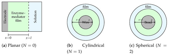
The bioanode consists of a conducting electrode core coated with an enzyme–mediator film of thickness l. The film contains glucose oxidase (GOx) and a redox mediator and is in contact with a well-mixed bulk solution that maintains the glucose concentration at . The operating principle is common to all three: glucose diffuses inward from the bulk solution and is oxidized by glucose oxidase within the film; the reduced enzyme is re-oxidized by the redox mediator; and the reduced mediator diffuses to the electrode, where it is re-oxidized and releases the electron that constitutes the cell current. Three configurations are considered, as illustrated in Figure 1.
Figure 1.
Schematic of the three bioanode configurations: (a) a planar enzyme–mediator film of thickness l on a flat electrode; (b) a cylindrical film coating a wire or fiber; and (c) a spherical film coating a particle. In every case, the electrode surface is at and the film/solution interface at . Substrate diffuses inward from the bulk solution, and the mediator shuttles electrons to the electrode. The three geometries are analyzed within a single generalized coordinate framework, the curvature being represented by the shape factor N (, 1, 2).
- 1.
- Planar. A flat electrode (for example, a screen-printed carbon or gold disc) is coated with a film of thickness l. Diffusion is one-dimensional along x, with at the electrode surface and at the film/solution interface.
- 2.
- Cylindrical. The film coats a wire or fiber (for example, a carbon fiber or platinum wire); diffusion is radial across the film, from the electrode surface at to the film/solution interface at .
- 3.
- Spherical. The film coats a spherical or quasi-spherical particle (for example, a nanoparticle-decorated bead); diffusion is again radial across the film of thickness l.
In all three cases, the electrode is located at and the bulk solution at . Following the established convention for reaction-diffusion in bounded catalytic films and pellets of general shape [5,6,8,9], the three geometries are treated within a single generalized coordinate framework in which the curvature is represented by the geometry (shape) factor N, taking for planar, for cylindrical, and for spherical films. The diffusion operator then takes the unified form
so that a single set of governing equations and a single closed-form solution describe all three geometries, the geometry entering only through N. This generalized-geometry formulation is the standard mathematical treatment adopted for chemically modified electrodes and catalytic films of planar, cylindrical, and spherical shape [5,8], in which the dimensionless film coordinate runs from the electrode () to the film/solution interface (); it is the basis of the present analysis.
It should be emphasized that this generalized-coordinate operator places the reference point at the axis of the cylinder () or the center of the sphere (), i.e., a line or a point of vanishing surface area, rather than at the finite-radius surface of a physical wire or bead electrode. Imposing the electrode condition at and evaluating the current from the mediator flux is therefore strictly physical only for the planar film (); for , the present treatment should be understood as a formal mathematical extension that reuses the same generalized operator and not as a faithful model of a curved electrode, whose physically rigorous description would place the electrode at a finite radius with the modified operator . Accordingly, the planar case is the physical model of this study, and the cylindrical and spherical cases are reported throughout as a generalized shape-factor extension of it. For a finite-radius electrode, the regular operator , with , replaces ; the curvature term then reads instead of , so relative to the present formal result, the correction is of order near the electrode. For the –10 typical of micro-wire and nanoparticle supports, this is a few-per-cent to order-unity modification of the curvature term, vanishing as (the planar limit); its quantitative treatment is left to future work.
The following assumptions are made: (i) the enzyme and mediator are uniformly distributed in the film; (ii) transport in the film is Fickian with constant effective diffusion coefficients and ; (iii) the substrate concentration at is fixed at ; (iv) the mediator cannot leave the film ( at ); (v) the mediator is oxidized at the electrode under Nernstian control; (vi) the system is isothermal, and film swelling and enzyme deactivation are neglected.
2.2. Transient Governing Equations
- Substrate Balance
- Mediator Balance
At the electrode, the current is produced by oxidation of the reduced mediator, and the current density is therefore proportional to the flux of reduced mediator at the surface,
Here, n is the number of electrons transferred, F is the Faraday constant, and is the roughness factor, defined as the ratio of the actual surface area to the projected (geometric) surface area; and denote the effective diffusion coefficients of the substrate and mediator within the film, respectively, and is the local rate of enzymatic turnover. The oxidized and reduced mediator forms are related by total mediator conservation within the film,
and are assumed to share the same effective diffusion coefficient . Differentiating Equation (12) then gives , so the current density can equivalently be expressed in terms of the oxidized-mediator field that is actually solved for,
The following dimensionless variables are introduced:
Here is the generalized dimensionless position coordinate, with the active electrode surface located at and the edge of the diffusion layer at , following the unified convention of Lyons [5] and Sivakumar et al. [8]. In this coordinate, the conservative operator and its expanded form coincide, and the shape factor recovers the planar, cylindrical, and spherical geometries, respectively; therefore denotes the radial/position coordinate of the generalized operator rather than a Cartesian film thickness.
The substrate and mediator are taken to have equal effective diffusion coefficients, , so that a single dimensionless time applies to both species; the mediator balance then requires no additional factor, and Equations (16) and (17) retain their symmetric form. In reality, and differ by about a factor of two (Table 1); the consequence of this idealization for the mediator response time is discussed in Section 6.
Table 1.
Representative physical quantities for a glucose-oxidase/redox-mediator bioanode and the resulting dimensionless groups. Values are order-of-magnitude estimates drawn from the enzyme-electrode literature, provided so that the dimensionless parameters can be mapped onto real systems; F, R, and T are the Faraday constant, gas constant, and temperature.
To relate the dimensionless groups to real enzymatic bioanodes, Table 1 lists representative physical quantities for a glucose-oxidase/redox-mediator electrode and the resulting values of , , , and . The parametric figures below scan ranges wider than these typical values to expose the full sensitivity.
The initial conditions for Equations (16) and (17) are
and the boundary conditions for Equations (16) and (17) are
The initial condition and the mediator surface condition are mutually incompatible at the single point . This corresponds to a step start-up: at , the electrode potential is applied instantaneously, so the oxidized-mediator fraction held at the electrode surface jumps from its initial value to the Nernstian value . The resulting corner discontinuity is integrable and is handled naturally by the solution method. In the semi-analytical expression (23), it is represented by the eigenfunction (Fourier) series, which converges to the imposed boundary value for every and reproduces the sharp initial transient as a sum of decaying exponential modes; in the numerical scheme, the boundary value is enforced for all , while the initial profile is prescribed at , so the discontinuity is confined to the first time level and does not affect the solution at later times. An identical remark applies to the substrate interface condition . The associated initial response is confined to a diffusive boundary layer of thickness ∼ at the electrode, so by , it spans only about one-fifth of the film; since the eigenfunction modes decay as , fewer than ten terms give three-figure convergence for , and the early-time planar results remain reliable.
The dimensionless current is given as
3. Analytical Approximations for Concentrations of Substrate and Mediator
Nonlinear equations are essential for describing many complex phenomena in areas such as physics, chemical engineering, biology, and applied mathematics. However, solving these equations remains a significant challenge because of their nonlinear nature. As a result, researchers have developed several iterative methods to obtain accurate approximate analytical solutions for nonlinear diffusion reaction problems. Some of the most commonly used techniques include “the Adomian Decomposition Method (ADM) [13], the Taylor Series Method (TSM), the Homotopy Perturbation Method (HPM), the Homotopy Analysis Method (HAM) [14], and the Variational Iteration Method (VIM) [15]”. These methods have been widely studied and successfully applied to a variety of nonlinear problems, demonstrating their effectiveness and reliability.
In the present study, the Laplace Homotopy Perturbation Method (LHPM) is employed to obtain an analytical approximation for the non-steady state nonlinear reaction–diffusion equations represented by Equations (16) and (17), together with the boundary conditions specified in Equations (19) and (20). The Homotopy Perturbation Method (HPM), originally proposed by Ji-Huan He, has become a widely recognized technique for solving highly nonlinear differential equations due to its simplicity and accuracy. By combining the Laplace transform with HPM, the LHPM enhances the solution process and provides highly accurate approximations over a wide range of parameter values with only a few iterations [7].
A notable advantage of LHPM is that it does not require the existence of a small perturbation parameter, allowing it to be applied to a broad class of nonlinear problems. Owing to this flexibility, the method has been successfully used to solve nonlinear partial differential equations arising in various scientific and engineering applications. For example, Mallikarjuna and Senthamarai [7] and Daniel et al. [13] applied LHPM to nonlinear models of immobilized enzyme systems, including batch reactors and microreactors. The method has also been effectively employed in studies involving gas dynamics [16], predator–prey systems [17], and fluid dynamics [18], demonstrating its versatility and reliability in handling complex nonlinear models. Related modelling and analysis of mediated enzyme-electrode and glucose biofuel-cell systems include the combined experimental and mathematical biofuel-cell model of Vasilenko et al. [19] and the mediated bioelectrocatalytic glucose-oxidation study of Noda et al. [20], which address the same class of coupled substrate–mediator kinetics considered here.
3.1. Deriving Semi-Analytical Expressions for the Non-Steady-State Equations (13) and (14) by Implementing the Laplace Homotopy Perturbation Method (LHPM)
Utilizing the LHPM approach, the approximate analytical expression for the substrate concentration (16) (see Appendix A) is given as
similarly, for the mediator concentration in Equation (17), the approximate analytical expressions derived using LHPM are as follows:
where
In obtaining Equations (22) and (23), the nonlinear ping-pong consumption term of the governing equations is represented by the constant linearized moduli M and R, which carry the dependence on the Michaelis–Menten constants (, ) and the potential amplitude () into the solution. This reduces the coupled nonlinear reaction–diffusion system to a linear one, so the present expressions are semi-analytical approximations rather than exact solutions of the full nonlinear problem; their accuracy is not assumed but is quantified against the numerical solution of the original nonlinear equations in the following sections and is found to be good within the operating range considered. Because M and R are evaluated with the surface mediator fraction and held constant, the linearization underestimates the local nonlinearity wherever substrate is strongly depleted or oxidized mediator is locally scarce; its error therefore grows with the Thiele modulu and, in the transient regime, at early times. For the curved cases, the early time, wheere for the curved cases it is dominated by the closure. These arguments are validated in the following sections. closure (largest when z is large, i.e., at small ), the constant-modulus linearization contributing the smaller, planar part.
The geometry enters the concentration profiles only through the factor , which arises from the leading-order closure of the generalized radial operator in the Akbari–Ganji/HPM–Laplace construction (Appendix A), where the characteristic relation is closed with the small-argument approximation to give . The small-argument closure is accurate while , that is, ; the benchmark in Section 4.2 confirms that the resulting error stays below up to , and within the operating range of this study (, hence ), it is effectively exact. This closure is exact for the planar case () and provides a unified elementary approximation for the cylindrical and spherical geometries; the same -scaled hyperbolic form was used for all three shapes in the immobilized-enzyme study that the present work extends [8]. As noted above, this factor is the only way the geometry enters the solution: Equations (22) and (23) are the planar profiles with the modulus rescaled by , so the cylindrical and spherical expressions are a shape-factor rescaling of the planar result and are reported as the formal extension described in Section 2.1. The accuracy of the physical (planar, ) model is quantified against the numerical solution in Table 2 and Table 3.
Table 2.
Substrate concentration profiles in planar, cylindrical, and spherical systems: validation of the LHPM technique against numerical simulations for , , , , and .
Table 3.
Mediator concentration profiles in planar, cylindrical, and spherical systems: validation of the LHPM technique against numerical simulations for , , , , and .
3.2. Non-Steady Current Equation
The dimensionless current is obtained directly from the spatial gradient of the non-steady mediator concentration at the electrode, (Equation (21)). Differentiating Equation (23) term by term and evaluating at —noting that the series factor contributes at —gives
The same spatial factor has zero derivative at , so the mediator no-flux condition is satisfied term by term. Because the oxidized-mediator concentration decreases from its electrode value into the film, , so in Equation (21); the corresponding physical current is positive, and the magnitude is reported throughout. As with the concentration profiles, the current expression (25) is physical for the planar electrode (); for , it is the corresponding quantity of the formal shape-factor extension, the flux being evaluated at the coordinate origin .
4. Validation of Analytical Results
The Laplace Homotopy Perturbation Method (LHPM) was used to solve the governing equations, Equations (16) and (17), yielding the semi-analytical expressions for substrate and mediator concentrations shown in Equations (22) and (23). The accuracy and feasibility of this method are verified through direct comparison with numerical simulations. Table 2 and Table 3 represent the comparison of the LHPM solution of substrate and mediator concentration to the numerical simulation done using the Scilab software 2026.1.0. It can be seen that the maximum mean absolute relative deviation of the substrate is and for the mediator concentration is . For , the numerical columns are themselves obtained from the singular-origin operator, so Table 2 and Table 3 validate the formal shape-factor extension rather than a physical curved electrode.
4.1. Numerical Method
The nonlinear reaction-diffusion system, Equations (16) and (17), was solved by the method of lines. The film was discretized on a uniform grid of points; spatial derivatives were approximated by second-order central differences, and the generalized curvature term was evaluated at the symmetry point through its regular limit , obtained from L’Hôpital’s rule with the symmetry condition (equivalently the symmetry option of the MATLAB routine pdepe). The electrode value was imposed as a Dirichlet condition and the outer no-flux condition as a one-sided difference. The resulting stiff system of ordinary differential equations in was integrated with an implicit backward-differentiation scheme (ode15s/BDF) using absolute and relative tolerances of and . Grid and time-step independence were verified by halving the mesh spacing h and the tolerances, which changed the reported concentrations and currents by less than . With this scheme, the electrode boundary value is reproduced exactly, , correcting the earlier ta.
4.2. Benchmark Against the Exact Linearized Solution
The factor in Equations (22) and (23) originates from closing the characteristic relation with the small-argument approximation . Because the linearized problem itself admits exact elementary solutions, the error introduced by this closure can be separated from the error introduced by linearizing the ping-pong kinetics. For the linearized substrate operator with , , the exact steady solutions are
where is the modified Bessel function of the first kind. These are compared with the LHPM/ form and with the full nonlinear numerical solution. Table 4 reports the maximum error over for the cylinder and sphere, separated into the linearization component [(ii) exact-linear versus (i) nonlinear] and the closure component [(iii) LHPM versus (ii) exact-linear]. Each entry of Table 4, Table 5 and Table 6 is reported as the maximum pointwise deviation over the electrode, expressed as a percentage of the normalized concentration,
so that in Table 4 the linearization error is , the closure error is , and the total error is , where , , and denote the full nonlinear numerical, the exact linearized, and the LHPM/ solutions, respectively.
Table 4.
Separation of error sources for the substrate: maximum error over (per cent) of the exact linearized solution against the full nonlinear numerical solution (linearization error), of the LHPM/ approximation against the exact linearized solution (closure error), and their total, for the cylindrical () and spherical () operators at , , .
Table 5.
Maximum deviation (per cent of the normalized concentration) of the closed-form substrate solution from the full nonlinear numerical solution versus dimensionless time , at , , , .
Table 6.
Maximum deviation (per cent) versus Thiele modulus , at , , , .
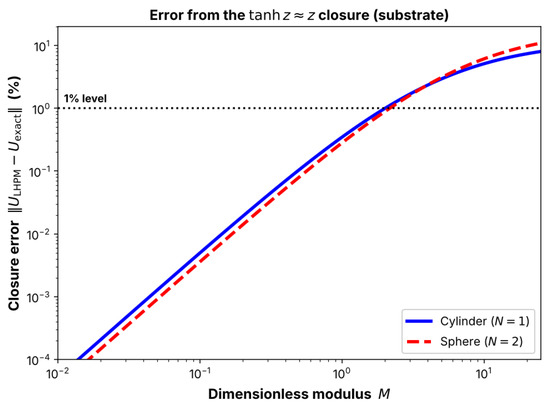
Throughout the operating range of the present study (, i.e., ), both components are below , and the closure contributes less than the kinetic linearization, so the approximation is not the limiting factor at the operating point. Figure 2 traces the closure error over a wider modulus range: it remains within up to and becomes appreciable only for (effective ), outside the physical regime considered here. This quantifies the range of validity of the unified closed form, replacing the earlier qualitative appeal to a “unified elementary closed form”.
Figure 2.
Error from the closure for the substrate: maximum deviation of the LHPM/ form from the exact linearized solution (modified Bessel for the cylinder, for the sphere) versus the linearized modulus M. The dotted line marks the error level; the operating range of the paper is , where the closure error stays well below . The comparison is at steady state; the kinetics enter only through M and the geometry only through the shape factor N.
Transient Accuracy and Validity Domain
The comparison above concerns the steady state; the transient regime and higher moduli are examined by mapping the maximum deviation of Equation (27), now evaluated between the time-dependent closed-form solution and the full nonlinear numerical solution , over dimensionless time and Thiele modulus. Table 5 lists this deviation against at the representative modulus , Table 6 against at , for the three shape factors.
For the planar electrode (), for which the closure is exact, the deviation is below for at all times and reflects only the kinetic linearization; solving the full coupled nonlinear system directly gives the same behavior, the linearization error reaching about at and at (). For the curved formal cases (), the agreement is within about for and for , but the series/closure error grows at early times (), consistent with the Laplace-domain observation that early times correspond to large s and hence large z, where is least accurate. Across the , , and ranges used in the discussion figures, the deviation changes by less than half a percentage point, being governed mainly by and N. The resulting validity domain is as follows: within about of the numerical solution for the planar electrode over at all (and for ), and within about 1– for the curved formal extension for ; at earlier times, or for , the deviation grows, and the planar numerical solution should be used as the reference.
Mapped onto the physical parameters of Table 1, the condition (equivalently ) spans the typical operating range of glucose-oxidase bioanodes (–2), so the constant-modulus linearization is adequate for the films and loadings listed there. It degrades as , and hence M, grows—through higher enzyme loading , thicker films (), a more active catalyst (larger ), or a lower substrate supply —and, for the curved cases, at early times () where the closure argument is largest. In those regimes, a fully nonlinear numerical treatment (the method of Section 4.1), or a higher-order homotopy correction that retains the next term of the perturbation series, becomes preferable to the leading-order closed form.
For the mediator, the exact-linear benchmark is not available in the curved cases: under the boundary conditions , , the regular solution of the linearized operator ( for , for ) cannot satisfy the outer no-flux condition, while the singular solution is excluded by the finite value imposed at the origin, so no bounded exact solution exists for . This is the analytical counterpart of the singular-origin limitation discussed in Section 2.1; the LHPM mediator expression is the exact planar solution with the modulus rescaled by and is retained as the formal shape-factor surrogate. The benchmark of this subsection therefore applies to the substrate, whose symmetric condition is regular at the origin for every N.
5. Result and Discussion
Throughout this section, the planar electrode () is the principal, numerically validated model, and it carries the physical interpretation of the results. Because the cylindrical and spherical solutions are the planar profiles rescaled by the single factor (Section 2.1), they are shown chiefly to illustrate the shape-factor formalism and are to be read as the formal extension rather than as models of specific curved electrodes; the discussion below therefore emphasizes the planar case and treats the curved curves as illustrative.
5.1. Spatiotemporal Evolution of Substrate and Mediator Fields
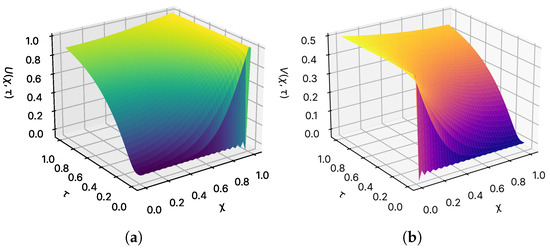
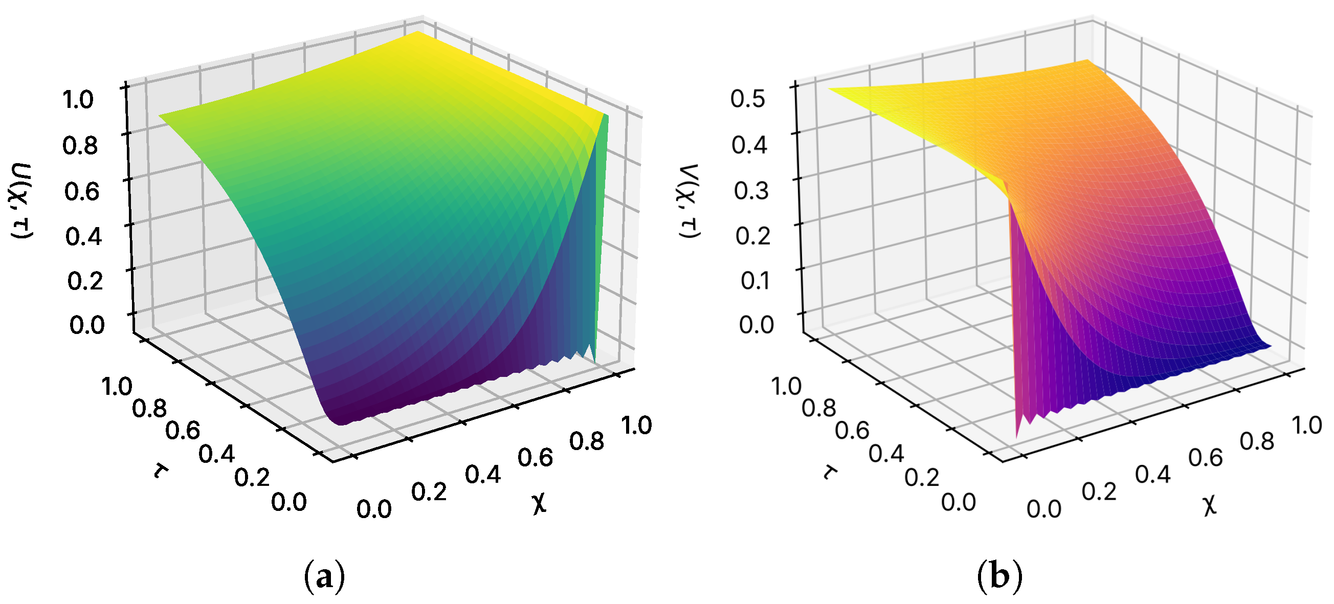
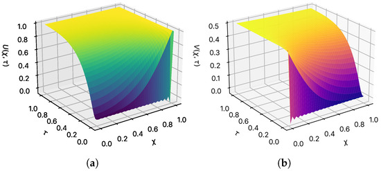
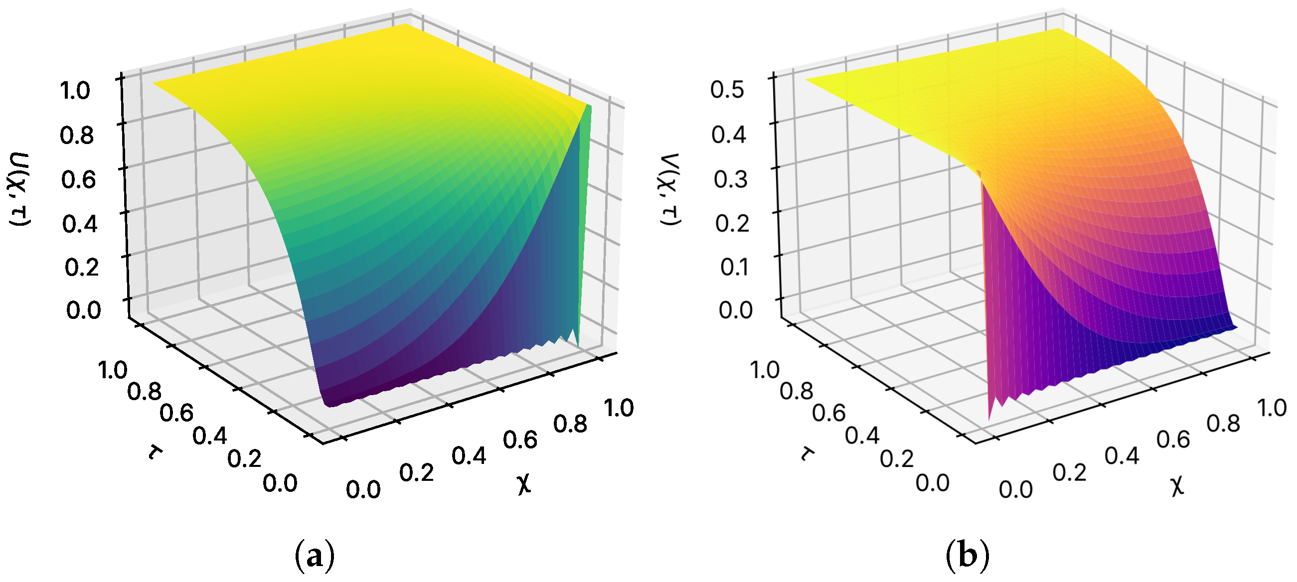
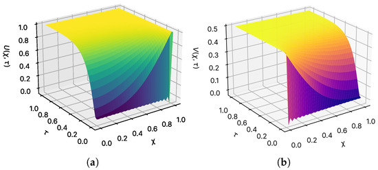
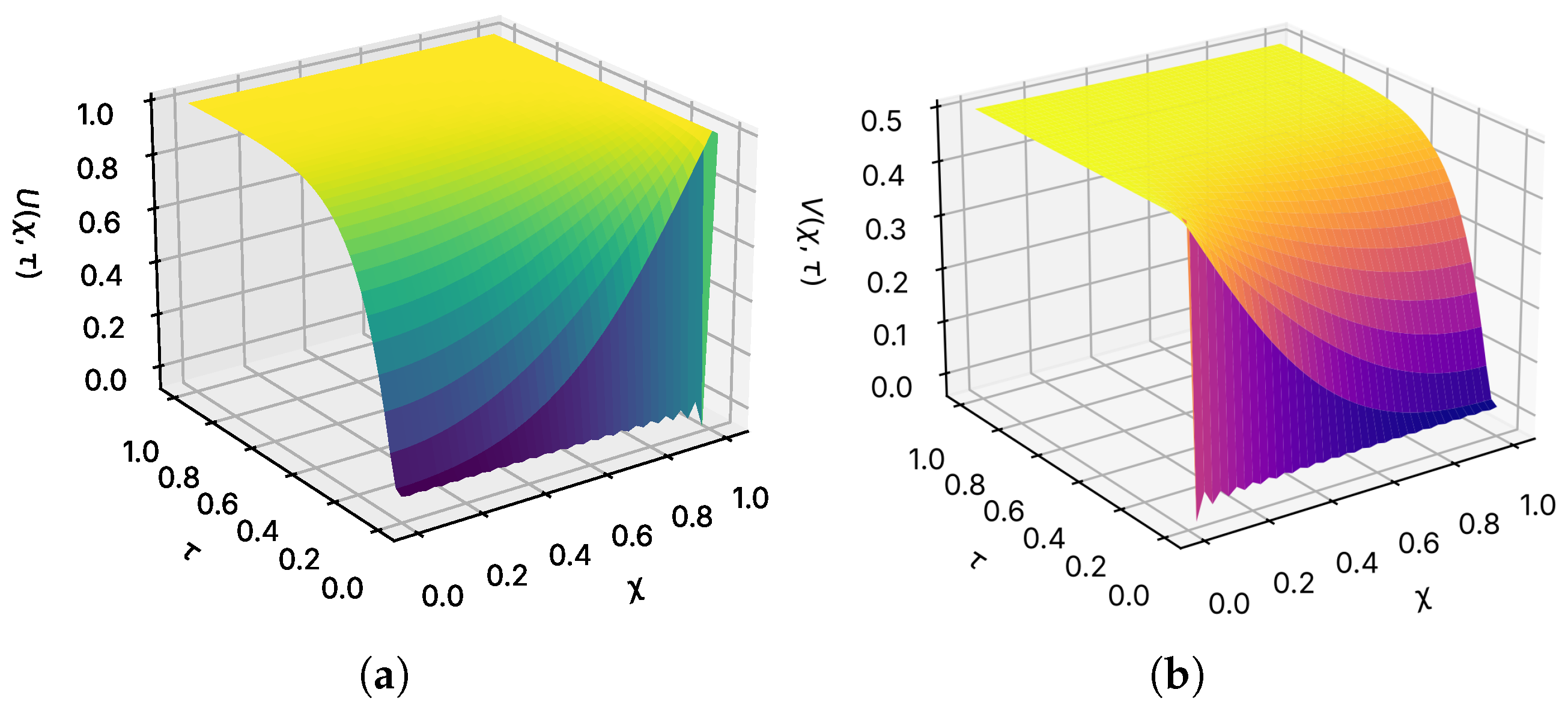
Figure 3, Figure 4 and Figure 5 show the evolution of the substrate and mediator concentration fields as functions of the dimensionless position and time for the planar, cylindrical, and spherical geometries. The substrate concentration increases with : it is lowest at the electrode surface (), where it is consumed by the enzymatic reaction, and recovers to its bulk value at the film/solution interface (). The steady-state substrate profiles are compared with the numerical solution in Table 2 for the operating condition , , , : the electrode-surface value is (planar), (cylindrical), and (spherical), corresponding to a surface depletion of about , , and , and the semi-analytical (LHPM) and numerical profiles agree to within a maximum mean absolute relative deviation of .
Figure 3.
Surface plots illustrating how dimensionless time and distance affect the concentrations of (a) substrate and (b) mediator within a planar geometry, when , , , for the shape factor (planar).
Figure 4.
Surface plots illustrating how dimensionless time and distance affect the concentrations of (a) substrate and (b) mediator within a cylindrical geometry, when , , , for the shape factor (cylindrical).
Figure 5.
Surface plots illustrating how dimensionless time and distance affect the concentrations of (a) substrate and (b) mediator within a spherical geometry, when , , , for the shape factor (spherical).
Starting from the initially reduced film (), the oxidized-mediator concentration rises monotonically in and stabilizes at the value fixed by the electrode potential, , where . The rise is monotonic at every position in the film, since the series solution, Equation (23), is a sum of same-signed decaying exponential modes. At steady state, the mediator field is nearly uniform: Table 3 shows that V varies by less than between and for all three geometries, with the LHPM and numerical results agreeing to within . Physically, mediator diffusion outruns enzymatic turnover, so the entire film thickness is electroactive and no inner region is starved of oxidized mediator; this is the regime in which the catalyst loading is fully utilized. The extent of mediator non-uniformity is governed by the mediator modulus : it is small when the Thiele modulus is modest and the mediator saturation parameter is large, which is the regime of the present figures, so the film stays close to uniform; raising or lowering increases R and localizes the reaction nearer the electrode.
5.2. Influence of Saturation Parameters , , and the Potential Amplitude
The Michaelis–Menten saturation parameters and enter the solution only through the linearized consumption modulus,
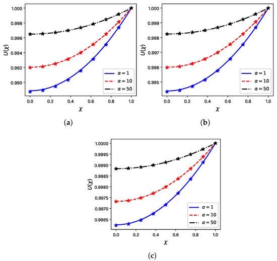
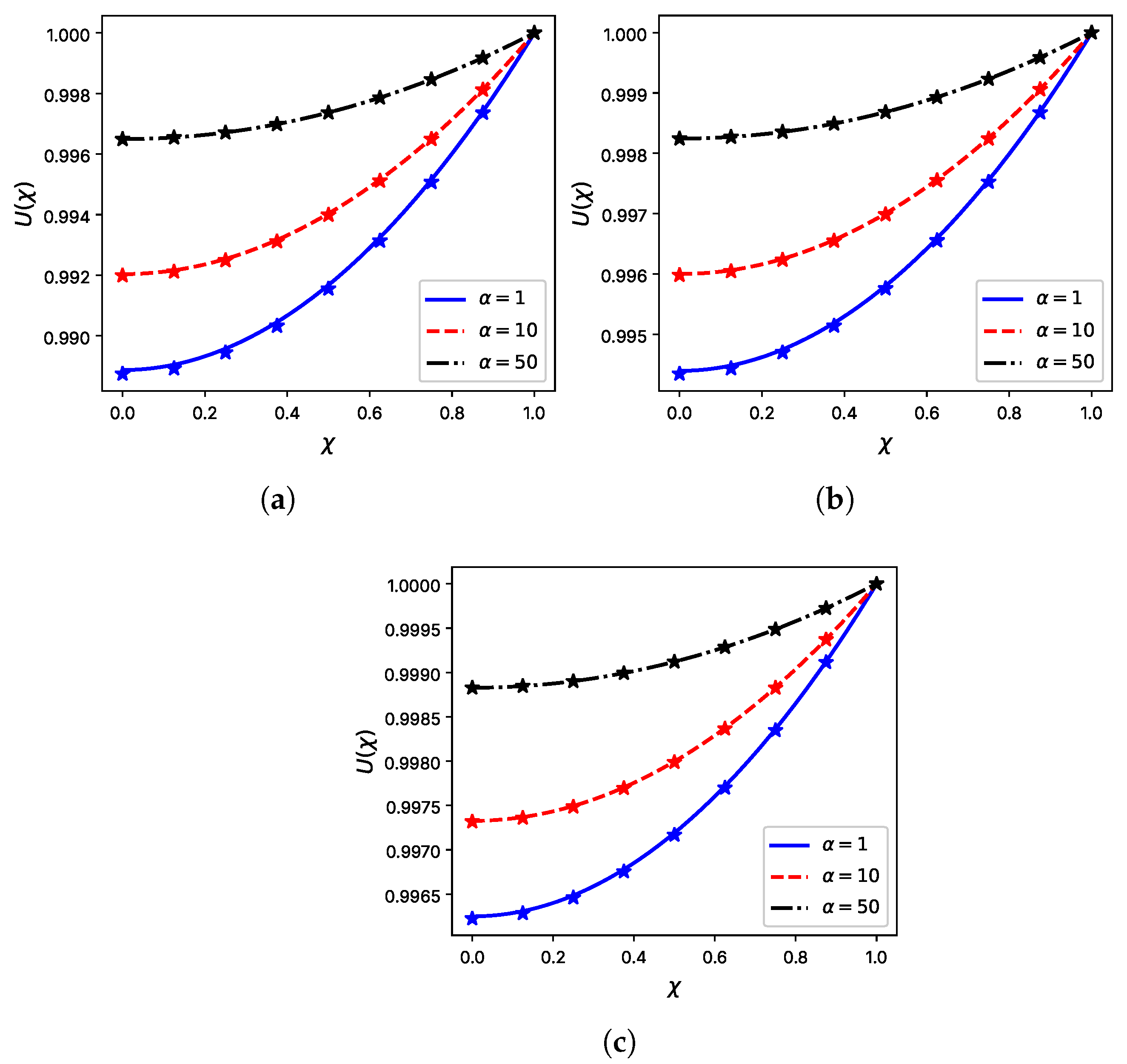
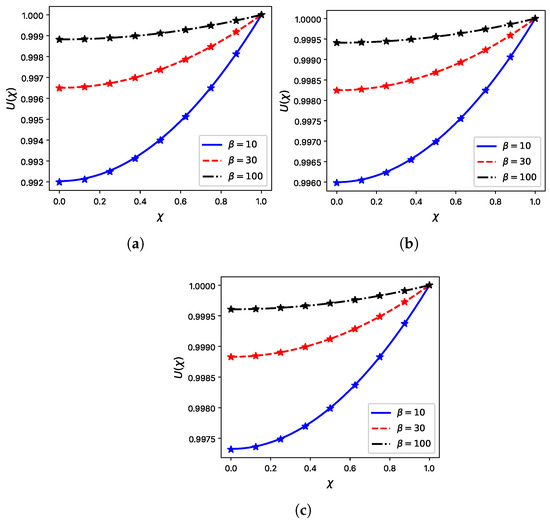
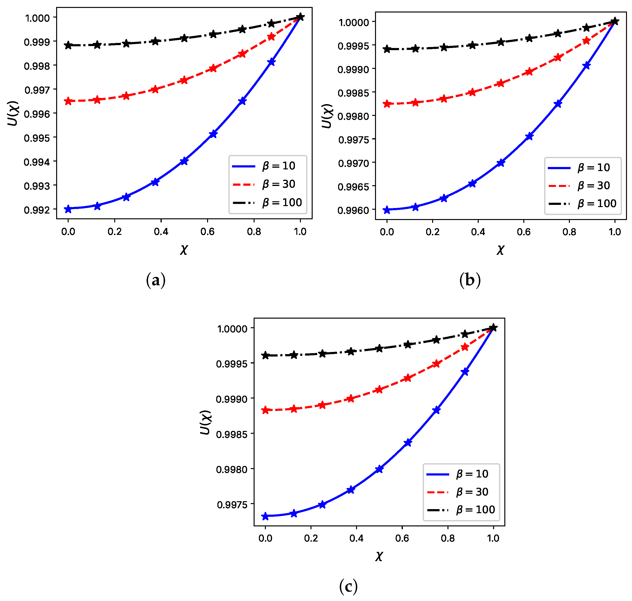
so raising either parameter reduces M, shortens the reaction penetration depth relative to the film thickness, and drives the substrate profile towards uniformity. Figure 6 and Figure 7 illustrate this common origin: the substrate depletion at the electrode is deepest in the strongly reacting limit and flattens progressively as or is increased, with the cylindrical and spherical panels exhibiting the same qualitative trend.
Figure 6.
Dimensionless substrate concentration profiles versus dimensionless radial distance across planar ((a), ), cylindrical ((b), ), and spherical ((c), ) geometries. The plots evaluate the impact of varying under fixed conditions (, , ; steady-state profiles). In each panel the three solid lines (of differing colour and style) are the numerical solutions for as labelled on the figure, and the markers “” are the corresponding LHPM solutions.
Figure 7.
Dimensionless substrate concentration profiles versus dimensionless radial distance across planar ((a), ), cylindrical ((b), ), and spherical ((c), ) geometries. The plots evaluate the impact of varying under fixed conditions (, , ; steady-state profiles). In each panel the three solid lines (of differing colour and style) are the numerical solutions for as labelled on the figure, and the markers “” are the corresponding LHPM solutions.
Although and are the governing saturation parameters, they are not interchangeable. Because the modulus depends reciprocally on the saturation groups, , the concentration fields are far more sensitive to these parameters at small values than at large ones: a fixed decrement in near zero produces a disproportionately large rise in M so that successive small- profiles separate into widely spaced, near-parallel traces rather than converging. The same reciprocal dependence makes the mediator field especially responsive at small ; because the mediator is consumed two-to-one per turnover, its modulus R is the larger of the two, and small changes in translate into large, nearly uniform shifts of the whole profile. In the opposite limit, the behavior becomes uninformative: as the saturation parameters grow, M tends to a constant, and the profiles collapse onto the flat, fully utilized limit already captured by the small-modulus analysis so that this regime is omitted from the figures as it adds no distinguishing feature beyond the cases shown.
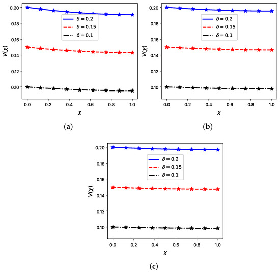
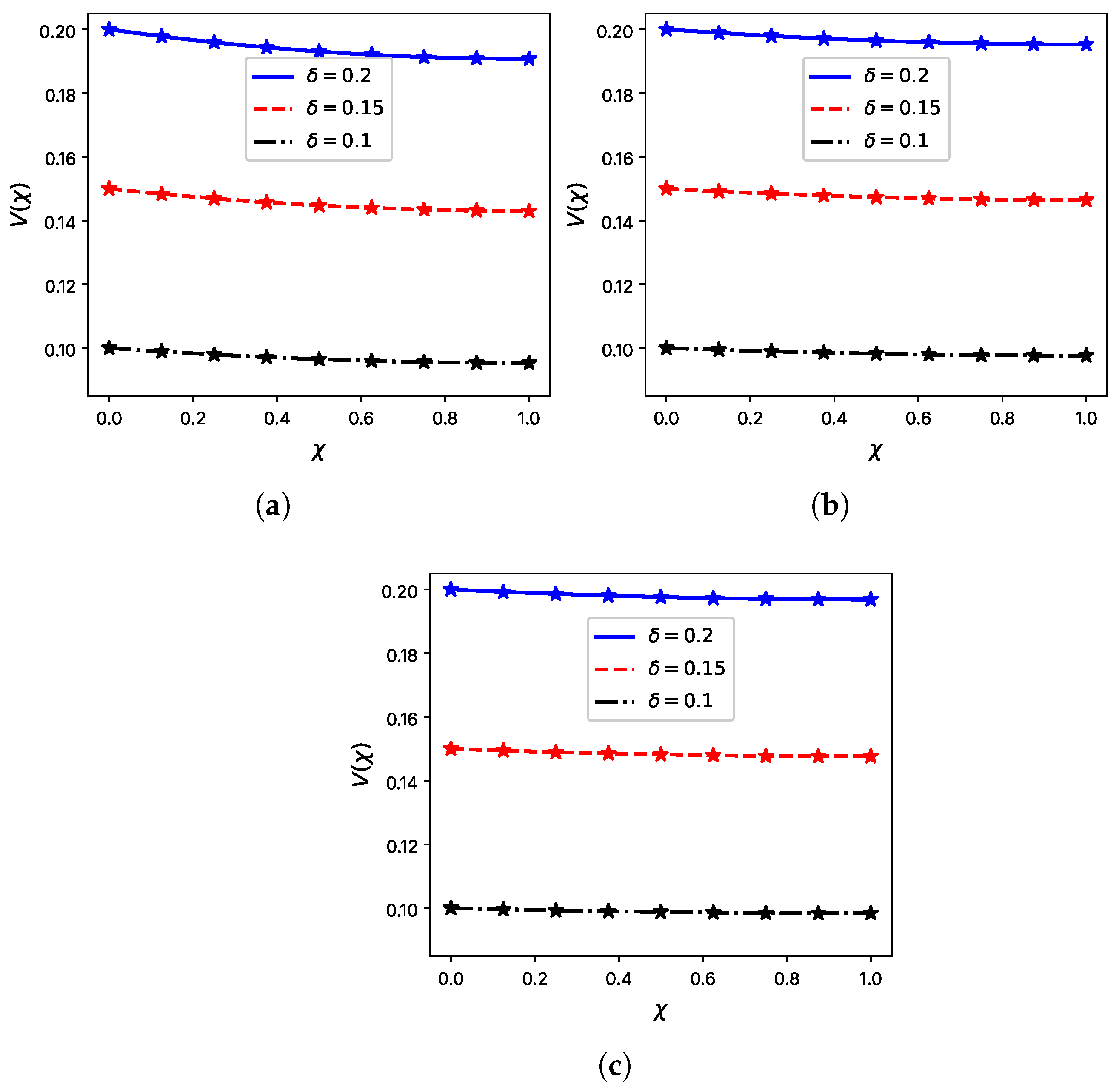
The potential amplitude enters the problem on a different footing. Rather than rescaling the modulus, it fixes the oxidized mediator fraction held at the electrode surface, and Figure 8 represents the structural prediction of Equation (23) that acts as a pure amplitude; the profiles for are geometrically similar, each decaying by a comparable relative amount while scaling in magnitude with itself. The sigmoidal form of also delimits the useful potential window. For , one has and further oxidative bias yields diminishing returns while accelerating mediator leaching and enzyme denaturation; for , , the film is starved for oxidized mediator irrespective of glucose supply. The steepest gain in current per volt occurs near at the formal potential of the redox couple, where operating an enzymatic biofuel cell also maximizes cell voltage. The model thus reconciles two design objectives that are often traded against one another.
Figure 8.
Dimensionless mediator concentration for , , and varying (steady-state profiles) across planar ((a), ), cylindrical ((b), ), and spherical ((c), ) geometries versus the dimensionless radial distance . In each panel the three solid lines (of differing colour and style) are the numerical solutions for as labelled on the figure, and the markers “” are the corresponding LHPM solutions.
5.3. Effect of Current Potential
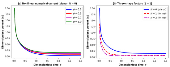
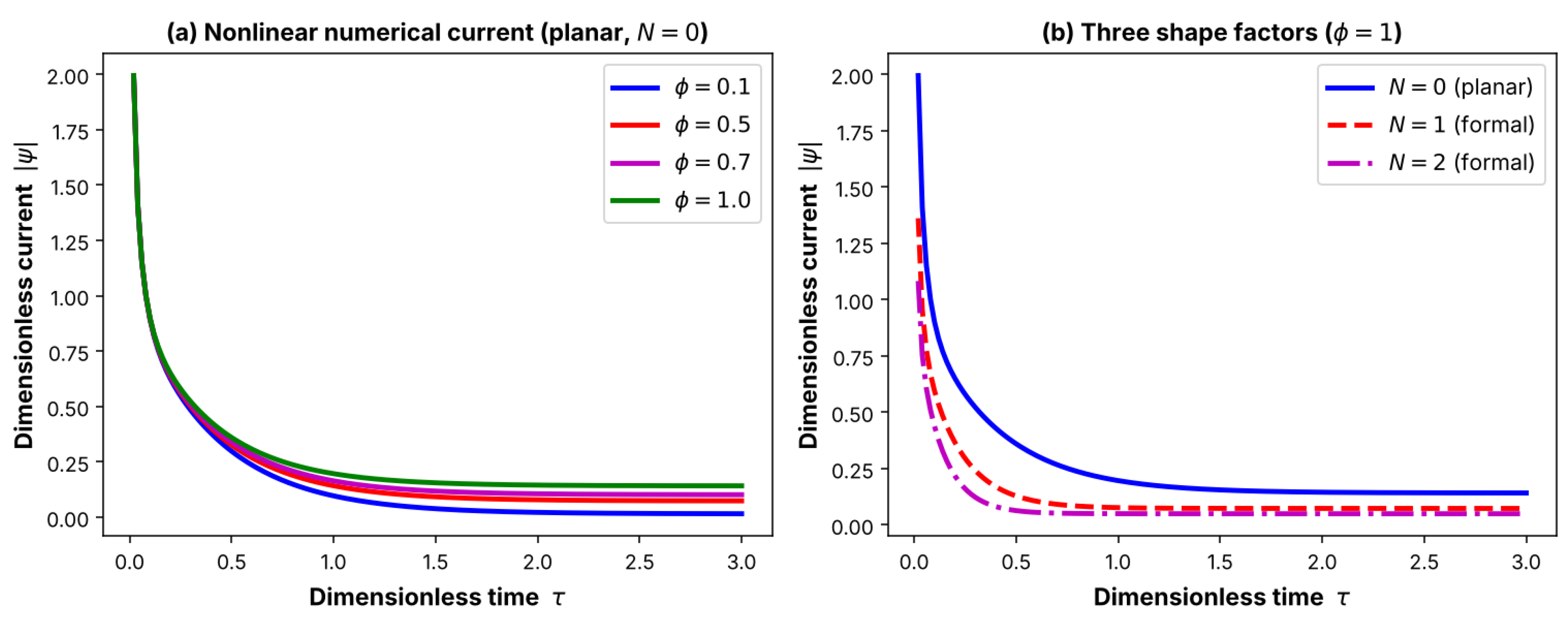
Figure 9 traces the dimensionless current magnitude against time . Starting from the initially unloaded film (), the oxidized-mediator gradient at the electrode is steepest immediately after the potential step, so the current is largest at short times and then relaxes monotonically to a steady value as the film fills—a Cottrell-type amperometric response. The relaxation is monotonic and free of overshoot: in the current series, Equation (25), every transient term carries the common factor together with the strictly positive quantities , and , where , and each relaxes as ; the steady term is likewise negative. Hence is a sum of same-signed, monotonically decaying modes for every shape factor and all admissible and , so no sign change—and therefore no overshoot—can occur. Because a linearized solution cannot by itself exclude overshoot of the nonlinear system, the full nonlinear numerical current was also computed for all three geometries (Figure 9); it is monotonic in every case, confirming the absence of overshoot in the nonlinear problem. The steady current magnitude increases with the Thiele modulus, from at to at for the planar electrode, since a larger modulus—whether from higher enzyme loading, a thicker film, or a more active catalyst—drives more substrate through the ping-pong cycle, regenerates more reduced mediator, and delivers a larger oxidized-mediator flux to the electrode.
Figure 9.
Transient dimensionless current magnitude versus time . (a) Planar electrode (), full nonlinear numerical solution for (, , ); (b) the three shape factors at , showing the planar nonlinear current together with the closed-form currents of the cylindrical and spherical formal extensions. In every case, the current is largest at start-up and decays monotonically to its steady value, with no overshoot.
6. Conclusions
In this study, a mathematical model was formulated that takes into account the effects of the enzyme reaction, mediator transport and diffusion, electrode potential, and electron transfer on the transient characteristics of an enzyme biofuel cells. The model consisted of the reaction-diffusion equations that were reduced to dimensionless form. The semi-analytical solution of these equations was obtained and compared with the numerical one. It is shown that the obtained agreement between analytical and numerical solutions justifies the correctness of the formulated model. In particular, the model adequately describes the time-dependent concentration profiles and current response of an enzyme biofuel cells. It is demonstrated that the processes of mediator diffusion and enzyme reaction are mutually dependent and should be considered when analyzing the electrochemical characteristics of the biosensor.
The electrode potential was found to have a strong effect on the current of the biofuel cell. The increase in electrode potential leads to an increase in the amount of oxidized mediator at the electrode surface and thus to an increase in the biofuel cell current. However, it was found that the dependence of the biofuel cell current on the electrode potential has a saturation shape. A higher electrode potential beyond a certain boundary does not lead to an increase in current due to mediator oxidation. The potential should be chosen based on the kinetics of the enzyme so that the most favorable conditions for the regeneration of the mediator are created without unnecessary energy costs for superfluous oxidation.
The analysis demonstrated that the Thiele modulus governs both the mediator concentration profile and the biofuel cell current, since it sets the balance between enzyme reaction and diffusion; a decreasing modulus marks the transition from a reaction-controlled to a diffusion-controlled regime, in which diffusion outpaces the enzymatic reaction and must therefore be accounted for in optimizing operating conditions. Overall, the proposed reaction–diffusion formulation—incorporating enzyme reaction, mediator diffusion and transfer, electrode potential, and charge transfer—adequately captures the transient behavior of the biofuel cells, showing that the current is governed by mediator oxidation at the electrode surface and that the applied electrode potential is critical to optimal operation. By treating reaction and diffusion as a coupled whole, the formulation offers a reliable basis for predicting and optimizing the planar enzyme biofuel cell electrode in practical applications. The planar configuration is the physical model validated here; the cylindrical and spherical results are reported as a formal generalized shape-factor extension, and a physically rigorous treatment of curved electrodes—placing the electrode at a finite radius with the operator —remains a natural direction for future work. Quantitatively, the closed-form solution matches the full nonlinear numerical solution to within about for the planar electrode for at all times and within 1– for the curved formal extension for ; the accuracy degrades at early times () and for , which delimits the domain of validity of the present approximation.
Two idealizations temper the quantitative response-time predictions. The substrate and mediator were assigned equal effective diffusivities, , whereas typical values differ by roughly a factor of two (Table 1, versus m2 s−1); since the mediator diffusion time then exceeds the substrate’s, unequal diffusivities would lengthen the mediator-limited response, so the predicted settling times (, i.e., ) are best read as order-of-magnitude estimates. The assumptions of uniform enzyme distribution, a non-swelling film and isothermal operation act similarly, affecting the absolute response time more than the qualitative trends. In design terms, the model indicates that the steady current is maximized by operating near the formal potential of the redox couple (where is most sensitive to the dimensionless potential ), that the current scales with the Thiele modulus until mass transport saturates it, and that the start-up time is set by the diffusion time —so thinner films respond faster at the cost of lower absolute current, a trade-off that the present closed-form expressions make explicit. In particular, the transient current relaxes with the dominant time constant , so the time to settle within of the steady current is for the planar electrode—scaling as the square of the film thickness and only weakly (through R) with enzyme loading—which gives a direct closed-form estimate of start-up time for design. These estimates apply within the stated domain of validity (, and for the curved formal results); outside it, a fully nonlinear treatment should be used.
Author Contributions
D.S. performed the data curation, prepared the original draft, and contributed to the visualization, formal analysis, and methodology. M.M. contributed to the formal analysis, methodology, software, and visualization. S.R. contributed to the methodology, validation, and resources, carried out the writing—review and editing, and supervised the study. S.A. contributed to the software and visualization. All authors have read and agreed to the published version of the manuscript.
Funding
This study received no dedicated funding from any public, commercial, or non-profit sector agencies.
Data Availability Statement
No data was used for the research described in the article.
Acknowledgments
The authors are deeply grateful to the SRM Institute of Science and Technology management for their continuous encouragement and motivation throughout this work.
Conflicts of Interest
The authors affirm that there are no conflicts of interest to disclose.
Nomenclature
| , , | Concentration of substrate, oxidized mediator, and enzyme (mol m−3) |
| Bulk substrate concentration (mol m−3) | |
| Reduced mediator concentration (mol m−3) | |
| Total mediator concentration (mol m−3) | |
| Dimensionless distance (spatial coordinate) | |
| Dimensionless time | |
| N | Geometry factor |
| , | Diffusion coefficient of substrate and mediator (m2 s−1) |
| , | Michaelis constant for substrate and mediator (mol m−3) |
| , | Reduced and oxidized enzymes |
| , | Reduced and oxidized mediator |
| Dimensionless non-steady substrate concentration | |
| Dimensionless non-steady oxidized mediator concentration | |
| Non-steady Thiele modulus | |
| Dimensionless non-steady substrate parameter | |
| Dimensionless non-steady mediator parameter | |
| Dimensionless potential parameter | |
| Dimensionless electrode potential | |
| Dimensionless current density | |
| p | Dimensionless power |
| LHPM | Laplace Homotopy Perturbation Method |
Appendix A. Estimating Time-Dependent Analytical Approximations for Concentrations of Substrate and Mediator
Constructing a homotopy relation corresponding to Equation (16), we obtain
by incorporating the boundary conditions in
The approximation solutions are obtained and given below
Substituting Equation (A2) into Equation (A1) and collecting terms of order , we derive
where . The Laplace transform of Equation (A3) results in
incorporating the relevant boundary conditions,
Applying the AGM, a trial solution for Equation (A4) is formulated to satisfy the prescribed initial and boundary conditions in Equation (A5),
where and we got the solution for as
Applying Equations (A8) to Equation (A4), wherein , we get
For sufficiently small z, we approximate by z; hence,
The residue calculation for Equation (A11) initiates at , where a simple pole is located. Additionally, solving the expression yields an infinite set of poles, which are expressed as
at s= 0,
residue at
Summing Equations (A13) and (A14) yields the total substrate concentration profile as expressed in Equation (22); following a similar approach, the semi-analytical formulations for the mediator concentration are established via the LHPM framework and are detailed in Equation (23).
References
- Goodenough, J.B. Electrochemical energy storage in a sustainable modern society. Energy Environ. Sci. 2014, 7, 14–18. [Google Scholar] [CrossRef] [Scilit]
- Ho, D.P.; Ngo, H.H.; Guo, W. A mini review on renewable sources for biofuel. Bioresour. Technol. 2014, 169, 742–749. [Google Scholar] [CrossRef] [Scilit]
- Gamella, M.; Koushanpour, A.; Katz, E. Biofuel cells—Activation of micro- and macro-electronic devices. Bioelectrochemistry 2018, 119, 33–42. [Google Scholar] [CrossRef] [Scilit]
- Nasar, A.; Perveen, R. Applications of enzymatic biofuel cells in bioelectronic devices—A review. Int. J. Hydrogen Energy 2019, 44, 15287–15312. [Google Scholar] [CrossRef] [Scilit]
- Lyons, M.E.G.; Salomi, R.J.; Rajendran, L. Formal analysis of isothermal reaction/diffusion in a defined general geometry. Int. J. Electrochem. Sci. 2023, 18, 100296. [Google Scholar] [CrossRef] [Scilit]
- Menaka, M.; Manimaran, R.; Saravanakumar, S.; Rajendran, L.; Eswari, A. Analyzing dead core formation in catalyst pellets of various geometries under non-isothermal conditions. Partial Differ. Equ. Appl. Math. 2025, 13, 101092. [Google Scholar] [CrossRef] [Scilit]
- Mallikarjuna, M.; Senthamarai, R. Mathematical analysis of batch reactor performance for the enzymatic synthesis of cephalexin: Laplace homotopy perturbation method and Adomian decomposition method. Partial Differ. Equ. Appl. Math. 2024, 11, 100806. [Google Scholar] [CrossRef] [Scilit]
- Sivakumar, M.; Mallikarjuna, M.; Senthamarai, R. A kinetic non-steady state analysis of immobilized enzyme systems with external mass transfer resistance. AIMS Math. 2024, 9, 18083–18102. [Google Scholar] [CrossRef] [Scilit]
- Krishnakumar, S.; Jeyabarathi, P.; Abukhaled, M.; Rajendran, L. Theoretical and numerical study of electrohydrodynamic flow in a planar, cylindrical, and spherical conduit. Int. J. Anal. Appl. 2024, 22, 158. [Google Scholar] [CrossRef] [Scilit]
- Albery, W.J.; Bartlett, P.N. Amperometric enzyme electrodes. Part I. Theory. J. Electroanal. Chem. Interfacial Electrochem. 1985, 194, 211–222. [Google Scholar] [CrossRef] [Scilit]
- Bartlett, P.N.; Pratt, K.F.E. Theoretical treatment of diffusion and kinetics in amperometric immobilized enzyme electrodes. Part I: Redox mediator entrapped within the film. J. Electroanal. Chem. 1995, 397, 61–78. [Google Scholar] [CrossRef] [Scilit]
- Rajalakshmi, R.; Marimuthu, A.; Naganathan, S.; Rajendran, L.; Izadi, M. Mathematical modeling and sensitivity analysis of enzymatic biofuel cells with various electrode geometries. J. Appl. Comput. Mech. 2025. [Google Scholar] [CrossRef]
- Daniel, S.; Mallikarjuna, M.; Senthamarai, R. Mathematical modeling and analysis of immobilized glucose dehydrogenase reactions in spherical microreactors. Eur. J. Pure Appl. Math. 2025, 18, 6203. [Google Scholar] [CrossRef] [Scilit]
- Liao, S. Beyond Perturbation: Introduction to the Homotopy Analysis Method; CRC Press: Boca Raton, FL, USA, 2003. [Google Scholar]
- He, J.H. Variational iteration method—A kind of non-linear analytical technique: Some examples. Int. J. Non-Linear Mech. 1999, 34, 699–708. [Google Scholar] [CrossRef] [Scilit]
- Johnston, S.J.; Hossein, J.; Moshokoa, S.P.; Ariyan, V.M.; Baleanu, D. Laplace homotopy perturbation method for Burgers equation with space- and time-fractional order. Open Phys. 2016, 14, 247–252. [Google Scholar] [CrossRef] [Scilit]
- Owolabi, K.M.; Pindza, E.; Karaagac, B.; Gulay, O. Laplace transform-homotopy perturbation method for fractional time diffusive predator–prey models in ecology. Partial Differ. Equ. Appl. Math. 2024, 9, 100607. [Google Scholar] [CrossRef] [Scilit]
- Aljahdaly, N.H.; Alweldi, A.M. On the modified Laplace homotopy perturbation method for solving damped modified Kawahara equation and its application in a fluid. Symmetry 2023, 15, 394. [Google Scholar] [CrossRef] [Scilit]
- Vasilenko, V.; Arkadeva, I.; Bogdanovskaya, V.; Sudarev, G.; Kalenov, S.; Vocciante, M.; Koltsova, E. Glucose-oxygen biofuel cell with biotic and abiotic catalysts: Experimental research and mathematical modeling. Energies 2020, 13, 5630. [Google Scholar] [CrossRef] [Scilit]
- Noda, T.; Wanibuchi, M.; Kitazumi, Y.; Tsujimura, S.; Shirai, O.; Yamamoto, M.; Kano, K. Diffusion-controlled detection of glucose with microelectrodes in mediated bioelectrocatalytic oxidation. Anal. Sci. 2013, 29, 279–281. [Google Scholar] [CrossRef] [Scilit]

Disclaimer/Publisher’s Note: The statements, opinions and data contained in all publications are solely those of the individual author(s) and contributor(s) and not of MDPI and/or the editor(s). MDPI and/or the editor(s) disclaim responsibility for any injury to people or property resulting from any ideas, methods, instructions or products referred to in the content. |
© 2026 by the authors. Published by MDPI on behalf of the International Institute of Knowledge Innovation and Invention. Licensee MDPI, Basel, Switzerland. This article is an open access article distributed under the terms and conditions of the Creative Commons Attribution (CC BY) license.