


Abstract
Virtual Coupling (VC) is an emerging railway signalling concept that allows successive trains to run closer together than the conventional absolute braking distance, promising higher line capacity. Prior VC research has mainly targeted controller design under a relative-braking assumption, leaving a gap in holistically defining and simulating VC scenarios across absolute and relative braking, and across inter-consist (train-to-train) and intra-consist (single-train splitting) configurations. This study addresses that gap by developing a longitudinal train dynamics model, deriving minimum-separation formulations for absolute and relative braking with a proposed dynamic safety margin, and designing a Model Predictive Control (MPC) train-following controller. Four operational scenarios, covering coupling and uncoupling at standstill and in motion, were simulated for a nine-car Class 390/0 Pendolino on the West Coast Main Line in the United Kingdom, between Rugby and Birmingham International. Relative-braking VC on a plain track reaches up to 240 trains per hour at a maximum headway of 15 s, whereas junction-constrained scenarios are capped at 60 trains per hour by the assumed switch-processing time, irrespective of braking principle. Absolute-braking VC achieves 60–70 trains per hour across scenarios. Splitting one train into a seven-car through-service and a two-car stopping portion reduced the through-service journey time by 27% and the combined energy consumption by 21.4% relative to an unsplit nine-car service.
1. Introduction
Railway transport occupies an increasingly important place among transport modes, a position reinforced by sustained investment and policy support from both governments and industry. The European Commission designated 2021 as the European Year of Rail to accelerate the shift toward rail and increase its share of the transport market [1]. Rail is also no longer regarded merely as an alternative to road transport: a UBS study anticipates that travellers will switch from air to high-speed rail in the post-COVID-19 period, driven by rail’s lower carbon emissions and the growing popularity of high-speed lines [2]. A more recent report on EU targets projects that high-speed rail traffic in the EU will double by 2030 and triple by 2050, through the construction of new lines and upgrades to the Trans-European Transport Network [3].
As rail networks become busier, bottleneck sections are reaching full occupancy, and conventional signalling leaves little room for further capacity growth [4,5]. Virtual Coupling (VC) has emerged as a potential solution to this problem and is increasingly discussed by both academia and industry. VC allows successive trains to run closer together than under conventional operation, by having them replicate each other’s acceleration and deceleration so that they move as a single unit. Extending the railway meaning of ‘coupling’—the physical connection between two cars or waggons—VC establishes this connection virtually between two or more trains. Given its novelty, VC has so far been the focus of only a small number of research efforts and dedicated projects, notably under the Shift2Rail Joint Undertaking within Horizon 2020. X2Rail-3 and MovingRail, both supported by Shift2Rail, are the best-known of these: MovingRail approached VC as a further evolution of ETCS Level 3, while X2Rail-3 examined it from a technology-independent perspective [6]. More recently, these Horizon 2020 initiatives have been followed by projects under the EU’s Europe’s Rail Joint Undertaking, such as R2DATO, under which DLR reported in 2025 the first real-world field trial of VC train-to-train communication, achieving centimetre-level distance measurement between two trains running 15–80 m apart [7], evidence that VC is moving from simulation toward field validation. In MovingRail, Aoun et al. [8] used the Delphi method to assess the impact of railway signalling innovations, comparing ETCS Level 3 moving-block signalling with VC across quantitative criteria (e.g., cost, capacity) and qualitative criteria (e.g., safety, regulatory approval) for high-speed, mainline, regional, urban and freight market segments. VC outperformed moving-block signalling overall, although technological maturity and safety concerns remain significant barriers to implementation. In a follow-up study, Aoun et al. [9] proposed a deployment-forecasting method based on SWOT and multi-criteria analysis of the same market segments, identifying gaps between current and future operational, technological and business states and laying out the actions and timelines needed for implementation; the results estimated that VC deployment could be completed by 2050 for every market segment under both optimistic and pessimistic scenarios, except for the mainline segment, whose pessimistic scenario extends slightly beyond 2050. Separately, X2Rail-3 deliverable D6.1 describes VC at a conceptual system level, defining its potential applications and operational scenarios; however, these scenarios are only described textually, without a corresponding performance assessment [10].
VC operations are expected to reduce headway times between trains and thereby increase line capacity, but this benefit needs to be quantified against conventional signalling and train control systems. Quaglietta et al. [11] developed a train-following model with distinct operational states—coupling, decoupling and coupled running—for VC signalling, and compared its capacity performance against ETCS Level 2, ETCS Level 3 and fixed-block signalling in a case study; VC delivered 77% and 43% shorter headways than ETCS Level 2 and Level 3, respectively. Similarly, Schumann [12] evaluated a VC scenario on the Tokyo–Osaka Shinkansen line through timetable analysis, finding that infrastructure factors—stopping patterns, platform length and track layout—affect VC performance, with results showing seating capacity increasing from 15,000 to 23,000.
Other studies approach VC from a different angle, focusing on the operational flexibility it offers for adjusting the number of carriages or splitting a long train into smaller units. Gallo et al. [13] proposed dynamically managing the number of carriages in a convoy, allowing trains to leave or pick up carriages parked in station sidings, with the aim of matching operational flexibility to dynamic passenger demand through mathematical programming. Qianqian and Hongwei [14] developed a leader–follower control mechanism based on artificial potential field theory to manage unbalanced passenger flow during rush hour on the Beijing Subway Batong Line, showing that VC can reduce capacity waste caused by tidal passenger flow and thereby improve service quality. Chen et al. [15] proposed an integrated train-scheduling method with a coupling strategy that decides whether a train should join a VC convoy, selecting operation level, departure time and arrival time through multi-objective optimisation that balances rescheduling under perturbations, the number of stranded passengers, and energy consumption. Wang et al. [16] proposed a method for calculating the carrying capacity of flexible train formations, comparing physically coupled and virtually coupled configurations, and found that VC-based variable formations have the smallest impact on carrying capacity while best addressing imbalances in passenger flow across regional rail networks.
A further strand of VC literature addresses controller design, drawing on a wide range of control methods; Xun et al. [17] provide a survey of these approaches. Controller design is one of the highest-priority challenges in VC implementation plans [9] for several reasons. First, low adhesion at the wheel–rail interface gives trains a longer braking distance than road vehicles, particularly at high speed [18,19]; because the friction between tyre and road is far higher, motorway vehicles can operate at a much shorter relative braking distance without the same safety concerns, whereas migrating from absolute to relative braking carries substantially more safety implications for rail. Second, unlike the motorway case—where a constant-time or constant-distance spacing policy simplifies controller design—the safe distance in rail is nonlinear and time-varying, since it depends on the braking capability of both trains in a pair. Su et al. [20] designed a control scheme for VC with heterogeneous braking capability based on a relative braking spacing principle, in contrast to the constant gap- and time-based policies common elsewhere [18,21], analysing the effect of heterogeneous braking dynamics on string stability in the frequency domain using Laplace transform; because braking capability varies throughout the journey with speed, adhesion, gradient and curvature, the safe distance must be continuously recalculated. Felez et al. [22] developed a decentralised robust MPC controller that explicitly accounts for uncertainty in train positioning and in adhesion-dependent braking capability, addressing a gap left by nominal MPC controllers, which do not consider such uncertainty and are therefore less robust when disturbances or errors significantly affect controller behaviour.
Overall, the reviewed literature shows a strong focus on controller design—MPC being the most widely adopted approach—together with related safety and anti-collision considerations, while studies addressing VC benefits such as operational flexibility and capacity enhancement have not defined or analysed VC operations in a holistic way; specific VC operational scenarios, in particular, have not yet been properly defined. This paper addresses that gap. The originality of this study lies in four contributions.
First, it defines a benchmark set of four VC operational scenarios—coupling and uncoupling, at standstill and in motion, on a plain line and at diverging, converging and combined junctions—and evaluates them on identical infrastructure, rolling stock, control parameters and safety-margin assumptions, so that the differences reported in separation, headway time and capacity are attributable to the scenario and the braking principle rather than to differences in the modelled system.
Second, it evaluates virtually coupled operation under the absolute braking principle as well as the relative one. Throughout the literature reviewed above, VC is defined in terms of relative braking; whether virtually coupled operation is achievable under absolute braking, and what it is worth in capacity terms, has not previously been established.
Third, it proposes a dynamic safety margin that scales with the instantaneous speed of the following train, in place of the constant, maximum-speed-based margin used in conventional moving-block practice. The results of Section 3 show that this margin, rather than the choice of braking principle alone, accounts for much of the separation reduction obtained under absolute braking.
Fourth, it extends Virtual Coupling from operation between separate trains to operation within a single train, by splitting one consist into a through portion and an intermediate-stopping portion under continuous VC control, and quantifies the resulting journey-time and energy benefits.
Table 1 sets this study against the Virtual Coupling research most closely related to it.
Table 1.
Position of this study relative to closely related Virtual Coupling research.
The remainder of this paper is organised as follows. Section 2 introduces the key operational concepts of Virtual Coupling and the methodology, including the mathematical modelling of vehicle dynamics under VC and the design of the train-following controller. Section 3 defines the case study, sets out the simulation inputs and the operational scenarios, and presents the results and findings, followed by a discussion of their implications for VC in Section 4. Section 5 concludes the paper with its contributions, limitations, and recommendations for future research.
2. Methodology
The methodology begins with the conceptual definitions of Virtual Coupling and continues with the mathematical modelling used to simulate them.
2.1. Conceptual Definition
Coupling requires, in general, an interaction between two objects. In railway terminology, coupling denotes the physical joining of two or more rail vehicles or consists into a single train, such that the coupled units move as one platoon at the same speed and acceleration at all times. The mechanical coupler is the device that establishes this connection and that acts as a bridge for the transfer of information between the coupled units; it performs two principal functions [10]:
- Maintaining a stable relative position between the coupled units by transferring push and pull forces;
- Transmitting braking and traction information between the coupled units, via wires or pipes, in a coordinated manner.
In this sense, VC denotes a form of interaction in which rail vehicles or trains are connected virtually rather than physically. The Virtual Coupling interaction (VCI) fulfils the two principal functions of the mechanical coupler through real-time collaboration between trains, exchanging vehicle dynamics data such as speed, acceleration and position over reliable communication and sensing systems [19]. VCI enables multiple trains to replicate one another’s motion in velocity and acceleration, so that they move as a single train. In a convoy, when the leading train accelerates or brakes, the follower or followers make the same change while in motion. How the virtual interaction is established depends on the communication topology—Vehicle-to-Vehicle (V2V) or Vehicle-to-Infrastructure-to-Vehicle—and on the underlying technology standard, such as 5G or ITS-G5 [23,24,25,26].
2.2. Mathematical Modelling
2.2.1. Longitudinal Vehicle Dynamics
Following Newton’s second law, longitudinal vehicle dynamics are mathematically modelled [27,28,29] as follows:
is the effective mass that carries the impact of rotational inertia on the vehicle mass; is the traction force of the vehicle, is the resistance force that is formulated with the Davis Equation (3); is the force exerted by gradient, is the vehicle mass, is the rotary allowance, typically below 0.2 depending on vehicle type [30]; A, B and C are the Davis coefficients, which depend on vehicle design [31], g is gravitational acceleration; and θ is the gradient angle.
The maximum tractive effort is confined by the normal force exerted from wheel to rail and adhesion, the friction coefficient between rail and wheel, as well as the proportion of powered axles, :
where g is the gravity rate. Following the tractive effort constraint, the maximum acceleration is expressed as follows:
In addition to the forward tractive effort, backward braking effort is required to decelerate the train. The braking effort is modelled with a constant braking rate as follows:
where b is the constant braking rate, taken as a positive magnitude, and is the braking effort.
The tractive effort has two regions—constant force and constant power region [32]:
- Horizontal/Constant Force region: The maximum effort is limited by adhesion, as given by Equation (5). Exceeding this value causes the wheels to slip.
- Curve/Constant Power region: Train power limits the tractive effort as per the formula: . Tractive effort therefore decreases as speed increases. is determined by the vehicle’s capability.
2.2.2. Train Motion Modes
Three motion modes of a typical train such as motoring, cruising and braking [33] are explained as follows: motoring is the stage when the train accelerates by applying tractive effort while cruising is defined as travel keeping a constant speed against an amount of tractive force that offsets the force exerted by gradient and rolling resistance. Braking is the deceleration stage to slow down and eventually halt the train. These modes are illustrated in Figure 1. Their mathematical explanations are tabulated in Table 2.
Figure 1.
Train motion modes. The diagram is schematic: it illustrates the sequence of motoring, cruising and braking between two stops rather than plotting a simulation output, so the axes carry quantities and units but no numerical scale. The line speed limit applied in the case study is the permissible-speed profile described in Section 3.1, which varies between 112 km/h and 200 km/h over the modelled section.
Table 2.
Motion mode equations.
2.2.3. Energy Consumption
Energy consumption is calculated as follows:
is journey time and is train power. The power equation is shown as follows:
When the power formula is inserted into (8), energy consumption is calculated with the following equation:
2.2.4. Braking Distance and Calculations
The braking principle is a critical factor in calculating the minimum distance between two trains. Two principles of braking are considered in this study (Figure 2).
Figure 2.
The minimum distance (dmin) between trains is determined by train velocity (v1 and v2) and braking principle.
Absolute braking (AB): The first train is considered as a fixed obstacle. Then, the minimum distance equals the follower train’s full braking distance plus safety margin.
where is the minimum distance, is the follower train’s speed, b2 is the follower train’s braking rate and SM is the safety margin. SM includes all system delays (onboard systems and communication latency) and is calculated as:
where is the total system delay.
Relative braking (RB): The first train is not treated as a fixed obstacle. When calculating the minimum distance, the first train’s speed becomes an input into the equation:
where is the minimum distance, is the follower train’s speed, is the leading train’s speed, is the follower train’s braking rate, is the first train’s braking rate and SM is the safety margin. As intuitively understood, can depend only on SM in the VC operation, in which and , if the trains are sufficiently homogenous. This result suggests that the safety margin (SM) merits closer analysis.
Safety Margin: Safety margin is employed to compensate for the delays in braking systems. Conventionally, SM is calculated as a constant value based on the maximum operational speed of the line [34,35]. This approach can be described as “constant safety margin”—thus, conservative. Following the introduction of VC concept, this study proposed a new one called “dynamic” safety margin with respect to the vehicle’s dynamic speeds.
Conventionally, SM is calculated as a constant value considering the maximum operational speed:
where is the maximum operational speed, is the inaccuracy of speed measurement, is the total system delay and is the location inaccuracy.
This constant formulation is conservative, since it applies the worst-case speed at every point of the journey. This study therefore proposes a dynamic safety margin, evaluated at the train’s instantaneous speed:
where is the instantaneous speed, is the inaccuracy of speed measurement, is the total system delay and is the location inaccuracy. The two formulations differ during acceleration and braking; in cruising mode, where the train runs at the line speed limit, they coincide. The elements of SM and their assumed values are given in Table 3.
Table 3.
Safety margin (SM) elements and values.
2.2.5. Controller Design for Train Following
Model Predictive Control (MPC) was selected from among several candidate methods, including adaptive PID, neural network and fuzzy control. MPC has been shown to outperform conventional PID control in comparable applications [21,36]. The controller was implemented in MATLAB/Simulink R2021a; its characteristics are described below.
MPC predicts the plant’s future behaviour through an online optimisation process [37]. At each time step, it solves an optimal control problem over a receding horizon, subject to the system’s constraints, to determine the next control action. The optimal input sequence over the control horizon is obtained by minimising a cost function defined by the control objectives over the prediction horizon. Only the first element of the optimal sequence is applied, and the optimisation is repeated at the following time step with updated measurements.
Control design has two objectives:
- To converge the intervehicle distance following error to zero:
- To converge the speed following error to zero:
State-Space Model:
The train’s longitudinal dynamics are nonlinear, owing to the motion resistance and the gradient force, which increases the complexity of the control design. However, because these terms are known at each step from the track data and the current speed, they can be treated as measured disturbances and incorporated into a linear plant model [38]. The train’s motion is therefore formulated as a linear state-space model with an additional disturbance input at each step:
The state variables of the plant are defined as with and where are, in order, the distance, speed of the follower train. The input and the output of the plant are, respectively, and with . The measured disturbance is .
The discretised model with as the sampling rate is designed as:
The model matrices are as follows:
Prediction Equation:
The prediction model enables one to predict a future state from the current measured system state, input and output. This is supported by the observability principle in control theory. Let the prediction horizon be and the controller horizon be , and and are prediction sequences of the system state and output within prediction horizon . Let be the system input sequence, i.e., the controller output sequence, within prediction horizon . Since , the system input is held constant for the remaining prediction horizon steps from through such that .
is the ith estimated step of the state vector at step k. The estimation values of the system state can be calculated through the following iterations:
The prediction sequences for the system output can be expressed as follows:
The prediction model in matrix form can be summarised as follows:
where , , , and .
Optimisation Problem
A quadratic objective function including inter-distance error and inter-velocity error is defined as:
where and are coefficients of the inter-distance and inter-velocity errors, respectively. The optimisation problem is solved via an active-set method that is a built-in algorithm in the MATLAB MPC Toolbox [38].
Constraints
The control parameters are subject to the following constraints:
Rail vehicle capability:
where is determined by the braking rate, and is determined by the acceleration rate. These parameters are limited by the vehicle design and capability.
Line speed limitation:
is the maximum operational speed depending on the train’s location. At each step k, the maximum allowable speed can change.
Safety Distance:
For safety-critical issues, cannot be less than at any time during the journey. In order to keep the distance within safe bounds, the small number is defined as:
If the trains are closer than , the follower train immediately applies braking. The MPC parameters used in this study are listed in Table 4.
Table 4.
MPC Parameters.
3. Case Study and Results
3.1. Case Study Setup and Simulation Inputs
Several operational scenarios were defined and tested in this study. The VC operational scenarios were constructed from the track data of the UK West Coast Main Line, between Rugby and Birmingham International in the English West Midlands. The track layout of the modelled section is shown in Figure 3. The speed limit profile is shown in Figure 4, and the altitude profile from which the gradient is derived in Figure 5; the section is 37 km long. The rolling stock modelled is the nine-car Class 390/0 Pendolino, whose parameters are listed in Table 5. The tractive effort and resistive force curve are shown in Figure 6. Tractive effort represents the longitudinal force delivered at the wheels and varies with train speed; the resistance curve is derived from the Davis equation, Equation (3). The maximum speed listed in Table 5 is the design speed of the class; the speed actually achieved in each simulation is governed by the line speed profile of Figure 4. Over the modelled section, the line speed limit varies between 112 km/h and 200 km/h (Figure 4), so the 225 km/h design speed of the class is never attained; simulated running speeds therefore lie within the range 0–200 km/h, with the trains at rest at the origin, at the intermediate station where one is modelled, and at the terminus. Both the speed limit and the gradient profile are tabulated over the full modelled section in Appendix A.
Figure 3.
Schematic track layout of the modelled West Coast Main Line section in the United Kingdom, between Birmingham International (0 km) and Rugby (37 km), showing the modelled turnouts, the intermediate station, and the extent of the section used by each operational scenario. The diagram is schematic and not to scale.
Figure 4.
Speed limitation profile.
Figure 5.
Altitude profile.
Table 5.
Simulation input data.
Figure 6.
Train tractive effort and resistance curve.
The rolling-stock parameters in Table 5 are taken from the published Class 390/0 traction dataset [39]. The adhesion coefficient and the proportion of powered axles were selected so that the adhesion limit of Equation (5) reproduces the constant-force tractive effort of that dataset: ρMgμ = 0.25 × 592.8 × 103 × 9.81 × 0.14 = 203.5 kN, against a published plateau of 203.7 kN. Correspondingly, the maximum power of 6000 kW at a tractive system efficiency of 85% gives 5100 kW at the wheel, against a published 5095 kW. Equations (5) and (6) therefore reproduce the traction–speed characteristic of the class through physically interpretable parameters rather than through a tabulated curve.
Three turnouts are represented, at 5 km (converging), 10 km (diverging) and 30 km (diverging), together with an intermediate station at 8.5 km. No single scenario uses all of them: OS1–OS3 and the intra-consist scenario run over the first 17 km of the section, whereas OS4 uses the full 37 km, and Figure 3 indicates which features each scenario activates. These are the track features represented in the simulation rather than a survey of the infrastructure in place on the section.
In the modelled system, conventional trackside interlocking is replaced by a train-borne track-resource allocation function forming part of the train-to-train communication-based signalling system: a train claims the track resource covering a turnout, holds it for the duration of its traversal, and releases it once clear, without a trackside interlocking granting the movement authority. The 60 s allocated to switch processing at each turnout in OS2–OS4 is the modelled proxy for that sequence, covering resource release by the leader, physical repositioning and detection of the switch, and resource claim by the follower. It is applied as a fixed value rather than derived from a specific interlocking or point-machine specification; the sensitivity of the junction capacity ceiling to it is identified as future work in Section 5.
Track curvature is not represented explicitly. The vehicle is modelled as a point mass in the longitudinal direction only (Section 2.2.1), so curve resistance does not appear in the resistance formulation of Equation (3) and no curve radii enter the simulation. Rochard and Schmid [31] omit curve resistance on the same grounds, noting that except for very tight curves of less than about 250 m radius its effect is small. Curvature is nevertheless present in the model through its operational effect: the speed limit profile of Figure 4 is the permissible-speed profile of the section, in which curve-imposed restrictions are already embedded, so trains are held to the same speed through curves as they would be on the real line. What is omitted is therefore the additional running resistance associated with curving, not the speed restriction itself.
To analyse VC operations more holistically, VC types are defined along two axes:
- View I—Safety Rule: Two types of VC, based on the braking principle:
- ○
- Absolute braking
- ○
- Relative braking.
- View II—Consist Formation: Two types, based on the consist formation:
- ○
- Between trains—inter-consist
- ○
- Between single rail units—intra-consist.
View I is based on the braking principles defined mathematically in Section 2.2.4. View II is based on whether the train is split into two or more shorter trains. The VC operational scenarios are given in Table 6. Four scenarios are defined from the possible combinations of coupling and uncoupling, and each is simulated under both View I and View II types. Taken together, these four scenarios constitute the benchmark set used throughout this study: a common set of operational cases against which the two braking principles and the two consist formations are compared on identical infrastructure, rolling stock, control parameters and safety-margin assumptions. Holding those inputs fixed is what makes the comparison a benchmark rather than a collection of individual simulations, since it ensures that differences in the reported separations, headway times and capacities are attributable to the scenario and the braking principle rather than to differences in the modelled system.
Table 6.
Virtual Coupling operational scenarios.
The simulation results are compared against one another on capacity performance. Hourly capacity for a given section is derived from the headway time between two consecutive trains [40], as given in Equation (34):
Headway time is the interval between two trains passing the same location consecutively. Line capacity is determined by the maximum headway time along the route, which identifies the weakest section of the line [40]; capacity generated elsewhere by shorter headways cannot be used by additional trains. A second comparison metric is the number of trains n required to operate the service at a given capacity, calculated as in Equation (35) [41]:
It is assumed that turnaround time is 180 s.
3.2. Inter-Consist VC Operations
The simulation results for inter-consist operations are analysed separately for the two braking principles. Results under the relative-braking principle are presented first, followed by the same operational scenarios under the absolute-braking principle.
3.2.1. Results for Relative Braking
The simulation results of each VC operational scenarios with RB principle are given in the following sections.
- Results for OS1 RB
In this scenario the trains begin their journey at the initial station and remain in VC mode throughout. Figure 7 shows the train motions as time–distance, speed–time and distance–speed plots, and Figure 8 shows the instantaneous headway time and distance. The headway time is longer near both the initial and the final station, because the trains are running below the maximum permitted speed in those regions. The headway distance shows the opposite pattern—shorter near the stations—because the minimum separation depends on the instantaneous speed; as the trains accelerate, the headway distance increases.
Figure 7.
OS1 RB Train Motion Outputs: (a) time–distance; (b) speed–time; (c) distance–speed.
Figure 8.
OS1 RB Capacity Outputs: (a) headway distance; (b) headway time.
Table 7 gives the performance outputs. Line capacity is set by the weakest section of the line, that is, by the longest headway time. OS1 RB achieves a line capacity of 240 tph, corresponding to more than 100,000 passengers per hour per direction (pphpd). Train 2 has a longer journey time than Train 1 because the required separation varies with the instantaneous speed: near the stations the minimum separation contracts, and Train 2 consequently reaches the final station later than the leading train. Train 2 consumes less energy than Train 1. The fleet size required to sustain this operation is 73 trains.
Table 7.
Performance outputs for OS1 RB.
- Results for OS2 RB
In the OS2 simulation, a turnout is located at 10 km, at which the follower diverges. A period of 60 s is allocated to switch processing for safety: the follower decouples from the leader and passes over the turnout one minute after the leader has cleared it. Figure 9 shows the train motions, and Figure 10 shows the instantaneous headway time and headway distance. The follower decouples from the leader at 227 s, at 6.82 km. Headway time and distance both increase towards the junction until the headway time reaches 60 s, equal to the time allocated to switch processing.
Figure 9.
OS2 RB Train Motion Outputs: (a) time–distance; (b) speed–time; (c) distance–speed.
Figure 10.
OS2 RB Capacity Outputs: (a) headway distance; (b) headway time.
Table 8 gives the performance outputs. Line capacity is limited by the weakest section, which is the junction area. OS2 RB achieves 60 tph, corresponding to more than 25,000 pphpd—a 75% reduction relative to OS1 RB. Train 2 consumes less energy than Train 1. The required fleet size is 17 trains, considerably fewer than for OS1 RB.
Table 8.
Performance outputs for OS2 RB.
- Results for OS3 RB
In this scenario, a turnout is located at 5 km, through which the follower converges onto the plain line. A period of 60 s is again allocated to switch processing: the follower enters the plain line one minute after the leader has cleared the turnout. Figure 11 shows the train motions and Figure 12 the headway time and distance. The follower begins the coupling manoeuvre at 240 s and 5 km, completing it 165 s later after 6.65 km. To enable coupling, the leader reduces speed to 30 m/s between 5 km and 10 km. This reduction is necessary because the two trains are homogeneous in tractive effort, so the follower could not otherwise close the gap. It is assumed that the leader’s slowdown is coordinated with the follower through the multi-agent VCI. The headway time falls from 60 s—the switch-processing allocation—to approximately 15 s once coupling is complete.
Figure 11.
OS3 RB Train Motion Outputs: (a) time–distance; (b) speed–time; (c) distance–speed.
Figure 12.
OS3 RB Capacity Outputs: (a) headway distance; (b) headway time.
Table 9 gives the performance outputs. Line capacity is limited by the junction area. OS3 RB achieves 60 tph, more than 25,000 pphpd: a 75% reduction relative to OS1 RB, and the same as OS2 RB. The required fleet size is 17 trains, the same as for OS2 RB.
Table 9.
Performance outputs for OS3 RB.
- Results for OS4 RB
This scenario combines OS2 and OS3. Two turnouts are placed at 5 km and 30 km. Unlike OS1–OS3, which use a 17 km section of the line, OS4 uses the full 37 km section, since demonstrating both the coupling and uncoupling manoeuvres within a single run required a longer distance than the other scenarios. The follower converges onto the plain line through the first turnout and later diverges through the second. A period of 60 s is allocated to switch processing at each: the follower enters the plain line one minute after the leader has cleared the first turnout and decouples and passes over the second turnout one minute after the leader has cleared it.
Figure 13 shows the train motions and Figure 14 the headway time and distance. The follower begins coupling at 240 s and, completing it 165 s later after 6.65 km. To enable coupling, the leader reduces speed to 30 m/s between 5 km and 10 km, for the reason given for OS3 RB, again assumed to be coordinated through the multi-agent VCI. The follower decouples from the leader at 749 s, at 26.8 km. The headway time falls from 60 s to approximately 15 s after coupling and rises again to 60 s as the second junction is approached.
Figure 13.
OS4 RB Train Motion Outputs: (a) time–distance; (b) speed–time; (c) distance–speed.
Figure 14.
OS4 RB Capacity Outputs: (a) headway distance; (b) headway time.
Table 10 gives the performance outputs. Line capacity is limited by the junction areas. OS4 RB achieves 60 tph, more than 25,000 pphpd: a 75% reduction relative to OS1 RB, and the same as OS2 RB and OS3 RB. The required fleet size is 17 trains, the same as for OS2 RB and OS3 RB.
Table 10.
Performance outputs for OS4 RB.
3.2.2. Results for Absolute Braking
The simulation results for VC operations under the absolute-braking principle are presented in this section. Each operational scenario from Section 3.2.1 is repeated under absolute braking.
- Results for OS1 AB
In this simulation, the trains begin their journey at the initial station and remain in VC mode throughout. Figure 15 shows the train motions and Figure 16 the instantaneous headway time and distance. As in OS1 RB, headway times are longer near the initial and final stations, where the trains run below the maximum permitted speed, while headway distances are shorter there, since the minimum separation depends on instantaneous speed. Table 11 gives the performance outputs. Line capacity is determined by the longest headway time along the route. OS1 AB achieves a line capacity of 70 tph, corresponding to more than 30,000 pphpd. Train 2 has a longer journey time than Train 1, for the reason given for OS1 RB, and consumes less energy. The required fleet size is 23 trains.
Figure 15.
OS1 AB Train Motion Outputs: (a) time–distance; (b) speed–time; (c) distance–speed.
Figure 16.
OS1 AB Capacity Outputs: (a) headway distance; (b) headway time.
Table 11.
Performance outputs for OS1 AB.
- Results for OS2 AB
In the OS2 AB simulation, a turnout is located at 10 km, at which the follower diverges from the plain line. A period of 60 s is allocated to switch processing: the follower decouples and passes over the turnout one minute after the leader has cleared it. Figure 17 shows the train motions and Figure 18 the headway time and distance. The follower decouples at 282 s, at 8 km. Headway time and distance increase towards the junction until the headway reaches 60 s, equal to the switch-processing allocation.
Figure 17.
OS2 AB Train Motion Outputs: (a) time–distance; (b) speed–time; (c) distance–speed.
Figure 18.
OS2 AB Capacity Outputs: (a) headway distance; (b) headway time.
Table 12 gives the performance outputs. Line capacity is limited by the junction area. OS2 AB achieves 60 tph, more than 25,000 pphpd—a reduction of approximately 14% relative to OS1 AB. Train 2 consumes less energy than Train 1. The required fleet size is 17 trains, comparable to OS1 AB.
Table 12.
Performance outputs for OS2 AB.
- Results for OS3 AB
In the OS3 AB simulation a turnout is located at 5 km, through which the follower converges onto the plain line one minute after the leader has cleared it. Figure 19 shows the train motions and Figure 20 the headway time and distance. The follower begins coupling at 240 s and 5 km, completing it 164 s later after 6.65 km. To enable coupling, the leader reduces speed to 30 m/s between 5 km and 10 km, for the reason given for OS3 RB, assumed to be coordinated through the multi-agent VCI. The headway time falls from 60 s to approximately 45 s once coupling is complete.
Figure 19.
OS3 AB Train Motion Outputs: (a) time–distance; (b) speed–time; (c) distance–speed.
Figure 20.
OS3 AB Capacity Outputs: (a) headway distance; (b) headway time.
Table 13 gives the performance outputs. Line capacity is limited by the junction area. OS3 AB achieves 60 tph, more than 25,000 pphpd: a reduction of approximately 14% relative to OS1 AB, and the same capacity as OS2 AB, OS2 RB and OS3 RB. The required fleet size is 17 trains, the same as for OS2 RB.
Table 13.
Performance outputs for OS3 AB.
- Results for OS4 AB
This scenario combines OS2 and OS3. Two turnouts are placed at 5 km and 30 km. Unlike OS1–OS3, which use a 17 km section of the line, OS4 uses the full 37 km section, since demonstrating both the coupling and uncoupling manoeuvres within a single run required a longer distance than the other scenarios. The follower converges onto the plain line through the first turnout and later diverges through the second, with 60 s allocated to switch processing at each.
Figure 21 shows the train motions and Figure 22 the headway time and distance. The follower begins coupling at 240 s, completing it 274 s later after 6.82 km. To enable coupling, the leader reduces speed to 30 m/s between 5 km and 10 km, assumed to be coordinated through the multi-agent VCI. The follower decouples at 802 s, at 28 km. The headway time falls from 60 s to approximately 15 s after coupling and rises again to 60 s as the second junction is approached.
Figure 21.
OS4 AB Train Motion Outputs: (a) time–distance; (b) speed–time; (c) distance–speed.
Figure 22.
OS4 AB Capacity Outputs: (a) headway distance; (b) headway time.
Table 14 gives the performance outputs. Line capacity is limited by the junction areas. OS4 AB achieves 60 tph, more than 25,000 pphpd: a reduction of approximately 14% relative to OS1 AB, and the same as every other scenario containing a junction. The required fleet size is 17 trains, the same as for OS2 RB and OS3 RB.
Table 14.
Performance outputs for OS4 AB.
3.3. Intra-Consist VC Operations
In an intra-consist operation, a single train is split into sub-trains that then run in VC mode. A Pendolino set has nine cars, which can be divided in several formations—1 + 8, 1 + 4 + 4, 2 + 5 + 2, and others. In effect, one physically coupled nine-car train becomes two virtually coupled trains. This allows an express service with few planned intermediate stops to detach carriages at specific stations without itself stopping, so that more destinations are served without adding stops to the through-service.
An intermediate station is placed at 8.5 km. The train is assumed to be divided into a two-car sub-train and a seven-car sub-train (2 + 7). The two-car sub-train runs as the follower and terminates at the intermediate station, while the seven-car sub-train runs as the leader and completes the journey to the final station. This scenario is simulated under the relative braking principle. The nine-car consist is divided pro rata by car count, giving a two-car sub-train of 131.7 t and 48.3 m and a seven-car sub-train of 461.1 t and 169.2 m. This assumes a uniform per-car mass and length; the driving cars of the real vehicle differ from the intermediate cars, so the division is an explicit modelling assumption rather than a vehicle specification.
Figure 23 shows the train motions as time–distance, speed–time and distance–speed plots, and Figure 24 shows the headway distance and headway time. The follower sub-train decouples from the leading sub-train at 223 s, at 6.7 km, after which the headway time and distance increase until the follower halts at the intermediate station. Table 15 gives the performance outputs.
Figure 23.
Intra-consist Operation Train Motion Outputs: (a) time–distance; (b) speed–time; (c) distance–speed.
Figure 24.
Intra-consist Capacity Outputs: (a) headway distance; (b) headway time.
Table 15.
Performance outputs for Intra-consist Operation.
The results indicate that intra-consist operation has the potential to reduce both journey time and energy consumption, because the sub-trains have lower masses and, in the case of the terminating portion, shorter journeys. Relative to an unsplit nine-car service with a journey time of 618 s and an energy consumption of 412 kWh, the split produces a 27% reduction in through-service journey time and a 21.4% reduction in combined energy consumption.
The intra-consist capacity of 225 tph is not directly comparable with the inter-consist figures, since it reflects shorter sub-train services rather than full-length runs. The reduction in journey time follows from the operational flexibility of the split: the leading sub-train (T1, seven cars) does not stop at the intermediate station and therefore reaches the final destination sooner than a conventional unsplit service. The reduction in energy consumption follows from two compounding effects. First, both sub-trains have a lower mass than the original nine-car consist, which reduces the traction energy—for each of them, consistent with the formulation in Section 2.2.1. Second, the two-car sub-train (T2) terminates at the intermediate station rather than running the full route, so it covers a shorter distance and consumes correspondingly less energy.
3.4. Sensitivity to Braking Rate and Adhesion
The results reported in Section 3.2 and Section 3.3 use a single constant braking rate, b = 0.675 m·s−2, and a single adhesion coefficient. Because the minimum-separation formulations of Equations (11) and (13) depend directly on the braking rate, and because braking capability in service varies with rail condition, the sensitivity of the reported separations and capacities to that value was examined. The analysis is carried out analytically on Equations (11), (13), (15) and (34) with the input data of Table 5 and is evaluated at the location along the route that sets line capacity for each braking principle. Under absolute braking, the headway time derived from Equation (11) increases monotonically with speed, so that location is the line-speed maximum of 200 km/h. Evaluated there, the procedure returns 69 tph against the 70 tph obtained from the simulation reported in Section 3.2.2, a difference of about one per cent, which validates the analytical treatment used in this section.
Four braking rates were examined, spanning the range reported for high-speed rolling stock. The rate modelled in this study, 0.675 m·s−2, is close to the 0.687 m·s−2 adopted for High Speed Two [42]. The same source reports the speed-dependent rates proposed by Hunyadi, of which the band covering 0–230 km/h gives 0.60 m·s−2, and adopts 0.50 m·s−2 once an allowance for accurate stopping and passenger comfort is included; that lower figure coincides with the service brake rate given for a comparable 600 t, nine-car, 200 km/h vehicle by Douglas et al. [32]. For degraded adhesion in bad weather, the same capacity study gives 0.30 m·s−2. For reference, trains operating over routes signalled in accordance with Appendix C of Railway Group Standard GKRT0075 are required to provide a nominal 9%g, or 0.883 m·s−2, full-service braking capability [43], so the rate modelled here is conservative relative to that requirement.
Table 16 gives the resulting minimum separation at line speed under both braking principles, together with the corresponding absolute-braking line capacity, and Figure 25 plots both against the braking rate. The two principles respond very differently. Under absolute braking, the minimum separation is dominated by the follower’s full braking distance and therefore scales inversely with the braking rate: it grows from 2664 m at 0.675 m·s−2 to 5667 m at 0.30 m·s−2, and the line capacity falls correspondingly from 69 tph to 34 tph. Under relative braking, Equation (13) subtracts the leading train’s braking distance from that of the follower; for a homogeneous convoy running at matched speed, the two braking terms cancel identically, and the minimum separation reduces to the safety margin of Equation (15), which contains no braking term. The relative-braking separation at line speed is therefore 263 m irrespective of the braking rate, and the ratio between the two principles widens from about 10:1 at the modelled rate to about 22:1 in the degraded case. Relative braking is thus not only the higher-capacity principle on the plain track but also the one whose separation is structurally insensitive to braking capability.
Table 16.
Sensitivity of minimum separation and line capacity to the braking rate, evaluated analytically at the 200 km/h line-speed maximum.
Figure 25.
Sensitivity to the braking rate at the 200 km/h line-speed maximum: (a) minimum separation under absolute and relative braking; (b) line capacity under absolute braking. Markers show the four cases of Table 16. The relative-braking separation is independent of the braking rate because the braking terms of Equation (13) cancel at matched speed; relative-braking line capacity is set on the station approaches rather than at line speed and is therefore not plotted in (b).
These rates can be related directly to wheel–rail adhesion. A deceleration of b requires an adhesion coefficient of at least b/g, so the 0.675 m·s−2 modelled here demands 6.9 per cent and the degraded case 3.1 per cent, as listed in Table 16. Recent experimental and numerical work on braking distance reports maximum adhesion coefficients of about 0.30 for dry clean rail, 0.20 for wet rail, 0.15 for moist and dirty rail and 0.10 for heavy contamination and finds no change in stopping distance for adhesion above 0.20, with a significant increase only below 0.15 [44]. Both the dry and the wet cases therefore supply considerably more adhesion than the modelled braking rate demands, which is why the capacities reported in Section 3.2 and Section 3.3 do not differ between dry and wet rail: over the normal range the braking rate is set by the braking system and by passenger comfort rather than by the available adhesion. Adhesion becomes the binding constraint only under heavy contamination, such as the autumn leaf-fall and winter ice conditions identified in the same study, and it is that regime rather than ordinary wet weather that the 0.30 m·s−2 case represents.
The same analysis bears on whether the braking rate should be treated as speed-dependent. The published speed-dependent characteristics resolve into distinct rates only above 230 km/h; below that speed a single value of 0.60 m·s−2 is quoted [42]. The section modelled here has a line-speed maximum of 200 km/h and, as stated in Section 3.1, running speeds lie within 0–200 km/h, so the entire simulated speed range falls inside that single band and a constant braking rate is appropriate for this case study. The value used lies slightly above the quoted band rate, and the 0.60 m·s−2 case in Table 16 brackets it: absolute-braking capacity would be 63 tph rather than 69 tph. Speed nevertheless influences the results strongly through the separation formulations themselves, since Equations (11) and (13) are quadratic in speed while the safety margin of Equation (15) is linear in it. This is why the binding location differs between the two principles: under absolute braking the headway time is greatest at the line-speed maximum, whereas under relative braking, where the quadratic terms cancel at matched speed, it is greatest on the station approaches, where the trains are not speed-matched and the cancellation is incomplete.
4. Discussion
Across all four operational scenarios, capacity was governed less by the braking principle itself than by whether a junction was present. On the plain-line scenario (OS1), relative braking reduced the maximum headway to a level that theoretically permits 240 tph—several times the throughput reported for fixed-block or conventional moving-block signalling on comparable corridors [11]—while absolute braking, after applying the dynamic, speed-dependent safety margin proposed in Section 2.2.4 in place of the conventional constant, maximum-speed-based margin, still reached 70 tph. Once a junction was introduced, whether diverging (OS2), converging (OS3) or both (OS4), capacity fell to 60 tph under both braking principles, set entirely by the assumed 60 s switch-processing time rather than by the minimum-separation formulations of Equations (14) and (15). The safety-margin advantage that relative braking provides on open track is, therefore, for a junction-dense corridor such as the West Coast Main Line, effectively erased at precisely the locations where additional capacity is most needed.
This pattern is consistent with, and extends, prior capacity assessments of VC. Quaglietta et al. [11] similarly found that when virtually coupled trains must diverge onto different routes, an absolute-braking separation has to be imposed at the junction, which can render VC’s capacity improvement over plain moving-block negligible—using ETCS Level 2 and Level 3 as the baseline rather than a dedicated VC controller. Aoun et al. [8] independently reported the same asymmetry for the mainline market segment: for diverging manoeuvres, VC and ETCS Level 3 yield an identical minimum headway of 53.3 s, whereas for plain-line non-stopping running, VC reduces the headway from 46.5 s to 12.3 s. The present results reproduce this qualitative pattern with an independently developed MPC-based train-following controller and add a quantitative benchmark specific to a Pendolino on the WCML: for this case study, junction handling—not the choice between absolute and relative braking—is the binding constraint on throughput. This suggests that infrastructure investment aimed at reducing switch-processing and route-setting time may yield a larger capacity return than migrating the braking principle alone.
The comparatively strong performance of absolute-braking VC on a plain track—70 tph, corresponding to a roughly 51 s headway via Equation (34)—is itself notable, since absolute braking is conventionally treated as the more conservative case. This appears to follow directly from replacing the constant, maximum-speed-based safety margin used in conventional moving-block practice [34,35] with the dynamic, instantaneous-speed-based margin proposed in this study (Equation (15)): because the margin shrinks whenever the train runs below line speed, absolute-braking headways are tightened during precisely the acceleration and braking phases where conventional practice is most conservative. This supports the paper’s stated aim of testing whether VC-style operation is achievable under absolute braking, rather than only under the relative-braking assumption that has dominated prior controller-design literature. A direct numerical comparison with the ETCS Level 3 headways reported elsewhere (for instance the 83 s maximum headway at the critical location reported by Quaglietta et al. [11] for trains sharing a route) cannot be drawn, since the case studies, rolling stock and infrastructure differ. Nonetheless, the magnitude of the tightening observed here indicates that the dynamic safety margin—and not relative braking alone—is a meaningful lever for capacity.
The sensitivity analysis of Section 3.4 adds a further distinction between the two braking principles. Because the leading train’s braking distance cancels from Equation (13) whenever the convoy is speed-matched, relative-braking separation is structurally independent of the braking rate, whereas absolute-braking separation scales inversely with it: degrading the rate from the modelled 0.675 m·s−2 to the 0.30 m·s−2 reported for bad-weather adhesion more than doubles the absolute-braking separation and halves its plain-line capacity, while leaving the relative-braking figure unchanged. Relative braking is therefore not only the higher-capacity principle on the plain track but also the more robust one under degraded rail conditions, an advantage that a single-point comparison cannot reveal and that partly offsets the junction-limited behaviour identified above.
The capacity figures reported in Section 3.2 are theoretical minimum-headway values for a homogeneous flow of identical trains, and are not directly comparable with a timetabled service. The section presently carries six trains per hour per direction, and no more than ten in any hour [45], so even the 60 tph junction ceiling lies an order of magnitude above what is operated today. That figure is not an input to the model, which derives capacity from the vehicle dynamics and the separation formulations alone, but it is the reference point against which these results should be read: on this corridor it is station calls, the speed differential between express and stopping services, junction margins and performance allowances that bind first, not the separation between successive trains. The results of Section 3.2 are therefore most usefully read as a comparison between braking principles under identical assumptions rather than as absolute capacity predictions.
The intra-consist scenario offers a different kind of benefit that inter-consist operation cannot: reductions in journey time and energy consumption for the same physical train. Splitting the nine-car Pendolino into a seven-car through-service and a two-car intermediate-stopping portion reduced the through-train’s journey time by 27% and the pair’s combined energy consumption by 21.4% relative to running the full nine-car set to both stops. Both effects trace back to the same mechanism: because traction energy—per Section 2.2.1—scales with train mass, and because the two-car portion covers a shorter distance, splitting removes both an unnecessary intermediate stop for the through-service and unnecessary mass and distance for the portion that does stop. This is conceptually related to, but operationally distinct from, the coupling/splitting studied by Schumann [12] for the Tokyo–Osaka Shinkansen, where capacity was gained by merging two physically separate services at a station rather than by splitting one physical consist mid-journey under continuous VC control. The present results suggest the same underlying principle—using VC to avoid unnecessary station dwell—extends from Schumann’s line-capacity focus to journey-time and energy benefits for express services with few intermediate stops, the class of service this scenario was designed to represent.
The vehicle model used here is deliberately a point mass, and Wu et al. identify precisely that simplification—representing a trainset as a single mass, which neglects in-train forces and nonlinearities in traction, braking, suspension and wheel–rail contact—answering it with high-fidelity vehicle system dynamics in which the simulation of each vehicle is assigned to an independent computer core [46]. That fidelity is what detailed assessments of train safety and vehicle-level performance require. The question addressed here is a different one: how minimum separation, and hence line capacity, responds to operational scenario and braking principle over a 37 km corridor. Equations (11), (13) and (15) depend on speed and braking rate rather than on intra-vehicle dynamics, so the factors recovered by higher-fidelity modelling enter these results only through the braking rate, whose influence is quantified in Section 3.4, while the point-mass formulation allows every scenario to be run over the full section at modest computational cost. The two approaches are therefore complementary, and the extension towards higher-fidelity dynamics is identified in Section 5.
Several scope limitations bear on how these figures should be read. First, both trains in every inter-consist scenario were modelled as identical Class 390/0 units with matched braking and tractive performance; a heterogeneous convoy—the case explicitly addressed by Su et al.’s heterogeneous-braking controller [20]—would require a continuously recalculated safety margin and would likely narrow the relative-braking advantage reported here. Second, the model adopts a constant braking rate and a constant adhesion coefficient, whereas braking capability in practice varies with speed, adhesion, gradient and curvature; the reported separations should therefore be read as first-order estimates. Section 3.4 quantifies the effect of that assumption: over the normal range of rail adhesion the modelled braking rate is limited by the braking system rather than by the available adhesion, so the reported capacities are insensitive to ordinary variation in rail condition, while the residual sensitivity of relative braking on the station approaches, where the trains are not speed-matched and the braking terms of Equation (13) do not fully cancel, is bounded by that argument rather than quantified. Third, only two trains were simulated in each inter-consist scenario, so string stability—a central concern for longer virtually coupled convoys—could not be assessed. Fourth, all scenarios assume ideal, disturbance-free operation and a fixed 60 s switch-processing time; since the reported 60 tph junction ceiling follows arithmetically from that assumption, a sensitivity analysis over the switch-processing time would be required before the figure is treated as a firm bound. Fifth, curvature enters the model only through the permissible-speed profile and not as a resistance term, since the point-mass longitudinal formulation omits curve resistance on the grounds set out in Section 3.1; curve radii for the section were not available, so the omission is bounded by that argument rather than quantified for this specific route. Sixth, the tractive-effort characteristic of Figure 6 is the nominal curve at rated line voltage, and catenary voltage is not represented in the model. Voltage depression under heavy traffic or towards the ends of an electrical section would reduce the tractive effort available, lengthening the acceleration phases and the coupling manoeuvres of Section 3.2—in which the leader already has to reduce speed for a homogeneous follower to close the gap—and hence the reported journey times. It would not alter the minimum-separation formulations of Equations (11)–(15), which depend on braking capability rather than on traction. Seventh, no driving margin below the permissible speed is modelled. The line speed enters the controller as the inequality constraint of Equation (31) rather than as a setpoint, and the objective function of Equation (29) minimises inter-distance and inter-velocity errors, so the follower tracks the leader rather than the limit; the trains are nonetheless free to run up to the permissible speed, whereas in practice a driver or an automatic train operation system holds a margin below it. The relationship between the two can be read directly from the distance–speed panel (c) of each train-motion figure—Figure 7, Figure 9, Figure 11, Figure 13, Figure 15, Figure 17, Figure 19, Figure 21 and Figure 23—which shows the line speed limit together with the speed actually achieved in that scenario. Modelling a driving margin would lengthen the reported journey times. It would not weaken the capacity comparison, however: the same speed profile is applied in every scenario, the junction-limited results of OS2–OS4 are set by the 60 s switch-processing time rather than by speed, and Section 3.4 shows that the absolute-braking headway of Equation (11) grows with speed, so running below the limit would shorten that headway rather than lengthen it.
5. Conclusions
This study developed a longitudinal train dynamics model, minimum-separation formulations for absolute and relative braking with a proposed dynamic safety margin, and an MPC-based train-following controller, and used them to simulate four Virtual Coupling operational scenarios—inter-consist and intra-consist, under absolute and relative braking—for a Class 390/0 Pendolino on the West Coast Main Line. Its contributions, set out in Section 1, are the benchmark set of operational scenarios evaluated on identical infrastructure, rolling stock and control parameters; the evaluation of virtually coupled operation under the absolute braking principle and not only the relative one; the dynamic, speed-dependent safety margin proposed in place of the conventional constant margin; and the extension of Virtual Coupling from operation between separate trains to operation within a single train. Across the four scenarios, capacity was governed primarily by the presence of a junction rather than by the choice of braking principle: relative braking on the plain track supported a theoretical 240 tph at a 15 s headway, but once trains had to diverge, converge, or both, capacity under both braking principles converged to 60 tph, set by the assumed 60 s switch-processing time rather than by the safe-separation formulations themselves. Absolute braking, aided by the proposed dynamic rather than constant safety margin, reached 60–70 tph across all scenarios. Splitting a single train into shorter sub-trains under intra-consist operation cut journey time by 27% and energy consumption by 21.4% relative to running the full consist, a benefit distinct from, and complementary to, the inter-consist capacity gains.
These results indicate that junction handling, rather than the choice between absolute and relative braking, is the binding constraint on VC’s capacity benefit for a junction-dense corridor such as the West Coast Main Line, and that a dynamic safety margin substantially narrows the performance gap between the two braking principles. The findings are subject to the scope limitations discussed in Section 4, including the assumption of homogeneous train performance and disturbance-free operation.
Future work should evaluate VC’s capacity benefit within a full network timetable rather than a single corridor, since gains are likely to be line-specific; test the sensitivity of the junction capacity ceiling to the assumed switch-processing time, and examine whether on-board interlocking can reduce it; extend the analysis to convoys of more than two trains, so that string stability can be assessed; and extend the vehicle model beyond a point-mass representation towards higher-fidelity multi-body dynamics, building on early work in this direction [46].
Author Contributions
Conceptualization, A.E., M.B. and C.R.; methodology, A.E. and L.C.; software, A.E.; validation, A.E. and M.Z.H.; formal analysis, A.E., M.B. and C.R.; investigation, A.E., M.B. and M.Z.H.; resources, A.E. and C.R.; data curation, A.E. and M.B.; writing—original draft preparation, A.E.; writing—review and editing, A.E., M.Z.H. and M.B.; visualisation, A.E.; supervision, M.B., L.C. and C.R. All authors have read and agreed to the published version of the manuscript.
Funding
This research was funded by the Republic of Türkiye Ministry of National Education, Ankara, Türkiye, through a YLSY-2015 PhD scholarship awarded to the first author.
Data Availability Statement
The track input data underpinning the simulations—the line speed limit and gradient profiles of the modelled West Coast Main Line section between Rugby and Birmingham International—are tabulated in full in Appendix A. The remaining original contributions presented in this study are included in the article. Further inquiries can be directed at the corresponding author.
Acknowledgments
During the preparation of this manuscript, the authors used Claude (Anthropic) Opus 5 model to assist with language editing and grammar and with consistency and sanity checks of equation, figure and table numbering, citation order, reference details and figure files. The study design, the simulation model, the results are entirely the authors’ own. The authors reviewed and edited all AI-assisted output and take full responsibility for the content of the publication.
Conflicts of Interest
The authors declare no conflicts of interest.
Abbreviations
The following abbreviations are used in this manuscript:
| AB | Absolute Braking |
| ETCS | European Train Control System |
| MPC | Model Predictive Control |
| OS | Operational Scenario |
| PID | Proportional–Integral–Derivative |
| RB | Relative Braking |
| SM | Safety Margin |
| V2V | Vehicle-to-Vehicle Communication |
| VC | Virtual Coupling |
| VCI | Virtual Coupling Interaction |
| WCML | West Coast Main Line |
Appendix A
The operational scenarios were constructed from the line speed limit and gradient profiles of the West Coast Main Line section between Rugby and Birmingham International, plotted in Figure 4 and Figure 5. Both are tabulated below over the 37 km modelled section, with chainage measured from the origin of the section at Rugby. Table A1 reproduces the speed limit profile exactly as a piecewise-constant function. Table A2 gives the gradient as a piecewise-constant approximation derived from the altitude profile; integrating it reproduces that profile to within 0.24 m over the full section, and segments whose gradient magnitude falls below 0.15 ‰ are reported as level.
Table A1.
Line speed limit profile of the modelled section.
Table A2.
Gradient profile of the modelled section.
References
- European Commission. Commission Proposes 2021 to Be the European Year of Rail. Available online: https://ec.europa.eu/commission/presscorner/detail/en/ip_20_364 (accessed on 4 June 2021).
- Railway Gazette News. UBS Predicts Post-Pandemic Shift from Air to High Speed Rail. Available online: https://www.railwaygazette.com/policy/ubs-predicts-post-pandemic-shift-from-air-to-high-speed-rail/56195.article (accessed on 4 June 2021).
- EU-Rail JU. Smart and Affordable Rail Services in the EU: A Socio-Economic and Environmental Study for High-Speed in 2030 and 2050; EU-Rail JU: Brussels, Belgium, 2023. [Google Scholar]
- RSSB. Rail Technical Strategy; RSSB: London, UK, 2020. [Google Scholar]
- UIC. Railway Technical Strategy Europe; UIC: Paris, France, 2019. [Google Scholar]
- X2Rail-3. Deliverable D7.5: Business Model; Hitachi Rail GTS Deutschland GmbH: Stuttgart, Germany, 2021. [Google Scholar]
- DLR Tests Virtual Coupling System in the Real World. Available online: https://www.dlr.de/en/latest/news/2025/dlr-tests-virtual-coupling-system-in-the-real-world (accessed on 25 July 2026).
- Aoun, J.; Quaglietta, E.; Goverde, R.M.P.; Scheidt, M.; Blumenfeld, M.; Jack, A.; Redfern, B. A Hybrid Delphi-AHP Multi-Criteria Analysis of Moving Block and Virtual Coupling Railway Signalling. Transp. Res. C Emerg. Technol. 2021, 129, 103250. [Google Scholar] [CrossRef] [Scilit]
- Aoun, J.; Quaglietta, E.; Goverde, R.M.P. Roadmap Development for the Deployment of Virtual Coupling in Railway Signalling. Technol. Forecast. Soc. Change 2023, 189, 122263. [Google Scholar] [CrossRef] [Scilit]
- X2Rail-3. Deliverable D6.1: Virtual Train Coupling System Concept and Application Conditions; Hitachi Rail GTS Deutschland GmbH: Stuttgart, Germany, 2020. [Google Scholar]
- Quaglietta, E.; Wang, M.; Goverde, R.M.P. A Multi-State Train-Following Model for the Analysis of Virtual Coupling Railway Operations. J. Rail Transp. Plan. Manag. 2020, 15, 100195, Erratum in J. Rail Transp. Plan. Manag. 2021, 17, 100237. [Google Scholar] [CrossRef] [Scilit]
- Schumann, T. Increase of Capacity on the Shinkansen High-Speed Line Using Virtual Coupling. Int. J. Transp. Dev. Integr. 2017, 1, 666–676. [Google Scholar] [CrossRef] [Scilit]
- Gallo, F.; Febbraro, A.D.; Giglio, D.; Sacco, N. A Mathematical Programming Model for the Management of Carriages in Virtually Coupled Trains. In Proceedings of the 2020 IEEE 23rd International Conference on Intelligent Transportation Systems (ITSC), Rhodes, Greece, 20–23 September 2020; pp. 1–6. [Google Scholar]
- Qianqian, Z.; Hongwei, W. A Multi-Train Cooperative Control Method of Urban Railway Transportation Based on Artificial Potential Field. In Proceedings of the 2019 Chinese Automation Congress (CAC), Hangzhou, China, 22–24 November 2019; pp. 1350–1355. [Google Scholar]
- Chen, C.; Zhu, L.; Wang, X. An Integrated Train Scheduling Optimization Approach for Virtual Coupling Trains. In Proceedings of the 2022 IEEE 25th International Conference on Intelligent Transportation Systems (ITSC), Macau, China, 8–12 October 2022; Volume 2022, pp. 2182–2186. [Google Scholar]
- Wang, Y.; Liu, L.; Liu, J.; Shi, J. Carrying Capacity Calculation Method of Regional Rail Transit Line Based on Flexible Train Formation. In Proceedings of the 2020 IEEE 23rd International Conference on Intelligent Transportation Systems (ITSC), Rhodes, Greece, 20–23 September 2020. [Google Scholar] [CrossRef] [Scilit]
- Xun, J.; Li, Y.; Liu, R.; Li, Y.; Liu, Y. A Survey on Control Methods for Virtual Coupling in Railway Operation. IEEE Open J. Intell. Transp. Syst. 2022, 3, 838–855. [Google Scholar] [CrossRef] [Scilit]
- Liu, Y.; Zhou, Y.; Su, S.; Xun, J.; Tang, T. An Analytical Optimal Control Approach for Virtually Coupled High-Speed Trains with Local and String Stability. Transp. Res. C Emerg. Technol. 2021, 125, 102886. [Google Scholar] [CrossRef] [Scilit]
- Stickel, S.; Schenker, M.; Dittus, H.; Unterhuber, P.; Canesi, S.; Riquier, V.; Ayuso, F.P.; Berbineau, M.; Goikoetxea, J. Technical Feasibility Analysis and Introduction Strategy of the Virtually Coupled Train Set Concept. Sci. Rep. 2022, 12, 4248. [Google Scholar] [CrossRef] [Scilit] [PubMed]
- Su, S.; She, J.; Wang, D.; Gong, S.; Zhou, Y. A Stabilized Virtual Coupling Scheme for a Train Set with Heterogeneous Braking Dynamics Capability. Transp. Res. C Emerg. Technol. 2023, 146, 103947. [Google Scholar] [CrossRef] [Scilit]
- Felez, J.; Kim, Y.; Borrelli, F. A Model Predictive Control Approach for Virtual Coupling in Railways. IEEE Trans. Intell. Transp. Syst. 2019, 20, 2728–2739. [Google Scholar] [CrossRef] [Scilit]
- Felez, J.; Vaquero-Serrano, M.A.; de Dios Sanz, J. A Robust Model Predictive Control for Virtual Coupling in Train Sets. Actuators 2022, 11, 372. [Google Scholar] [CrossRef] [Scilit]
- Unterhuber, P.; Lehner, A.; de Ponte Müller, F. Measurement and Analysis of ITS-G5 in Railway Environments. In Communication Technologies for Vehicles; Lecture Notes in Computer Science (Including Subseries Lecture Notes in Artificial Intelligence and Lecture Notes in Bioinformatics); Springer: Cham, Switzerland, 2016; Volume 9669, pp. 62–73. [Google Scholar]
- Homay, A.; de Sousa, M.; Almeida, L.; Martins, A.; Oliveira, E. Multi-Agent Based Uncoordinated Channel Hopping in the IEEE 802.15.4e. In Advances in Intelligent Systems and Computing; Springer: Cham, Switzerland, 2017; Volume 619, pp. 287–296. [Google Scholar]
- Gomez, A.A.; Mozo, E.; Bernado, L.; Zelenbaba, S.; Zemen, T.; Parrilla, F.; Alberdi, A. Performance Analysis of ITS-G5 for Smart Train Composition Coupling. In Proceedings of the 2018 16th International Conference on Intelligent Transportation Systems Telecommunications (ITST), Lisboa, Portugal, 15–17 October 2018. [Google Scholar]
- He, D.; Ai, B.; Guan, K.; García-Loygorri, J.M.; Tian, L.; Zhong, Z.; Hrovat, A. Influence of Typical Railway Objects in a mmWave Propagation Channel. IEEE Trans. Veh. Technol. 2018, 67, 2880–2892. [Google Scholar] [CrossRef] [Scilit]
- Zhou, K.; Song, S.; Xue, A.; You, K.; Wu, H. Smart Train Operation Algorithms Based on Expert Knowledge and Reinforcement Learning. IEEE Trans. Syst. Man. Cybern. Syst. 2022, 52, 716–727. [Google Scholar] [CrossRef] [Scilit]
- Wang, D.; Wu, J.; Wei, Y.; Chang, X.; Yin, H. Energy-Saving Operation in Urban Rail Transit: A Deep Reinforcement Learning Approach with Speed Optimization. Travel Behav. Soc. 2024, 36, 100796. [Google Scholar] [CrossRef] [Scilit]
- Jiang, K.; Tian, Z.; Hillmansen, S. Station-Centric Railway Intermittent Electrification Strategy for BEMU with Hybrid Power Supply. In Proceedings of the 2025 IEEE Transportation Electrification Conference and Expo, Asia-Pacific (ITEC Asia-Pacific), Singapore, 25–28 November 2025; pp. 1–5. [Google Scholar] [CrossRef] [Scilit]
- Steimel, A. Electric Traction-Motive Power and Energie Supply; Division Deutscher Industrieverlag: Essen, Germany, 2007. [Google Scholar]
- Rochard, B.P.; Schmid, F. A Review of Methods to Measure and Calculate Train Resistances. Proc. Inst. Mech. Eng. F J. Rail Rapid Transit 2000, 214, 185–199. [Google Scholar] [CrossRef] [Scilit]
- Douglas, H.; Schmid, F.; Roberts, C.; Hillmansen, S. Evaluation of Permanent Magnet Motor Energy Saving Technology for Different Types of Railways. In Proceedings of the 2016 IEEE International Conference on Intelligent Rail Transportation (ICIRT), Birmingham, UK, 23–25 August 2016; Institute of Electrical and Electronics Engineers Inc.: New York, NY, USA, 2016; pp. 123–129. [Google Scholar]
- Zhao, N.; Roberts, C.; Hillmansen, S.; Tian, Z.; Weston, P.; Chen, L. An Integrated Metro Operation Optimization to Minimize Energy Consumption. Transp. Res. C Emerg. Technol. 2017, 75, 168–182. [Google Scholar] [CrossRef] [Scilit]
- Durmus, M.S.; Ucak, K.; Oke, G.; Soylemez, M.T. Train Speed Control in Moving-Block Railway Systems: An Online Adaptive PD Controller Design. IFAC Proc. Vol. 2013, 46, 7–12. [Google Scholar] [CrossRef] [Scilit]
- European Railway Agency. Introduction to ETCS Braking Curves; European Railway Agency: Valenciennes, France, 2016. [Google Scholar]
- Salem, F.; Mosaad, M.I. A Comparison between MPC and Optimal PID Controllers: Case Studies. In Proceedings of the Michael Faraday IET International Summit 2015, Kolkata, India, 12–13 September 2015; Institution of Engineering and Technology: London, UK, 2015; pp. 59–65. [Google Scholar]
- Orukpe, P. Model Predictive Control Fundamentals. Niger. J. Technol. 2012, 31, 139–148. [Google Scholar]
- Bemporad, A.; Ricker, N.L.; Morari, M. Model Predictive Control Toolbox User’s Guide; MathWorks: Natick, MA, USA, 2023. [Google Scholar]
- Zhao, N.; Roberts, C.; Hillmansen, S. The Application of an Enhanced Brute Force Algorithm to Minimise Energy Costs and Train Delays for Differing Railway Train Control Systems. Proc. Inst. Mech. Eng. F J. Rail Rapid Transit 2014, 228, 158–168. [Google Scholar] [CrossRef] [Scilit]
- Abril, M.; Barber, F.; Ingolotti, L.; Salido, M.A.; Tormos, P.; Lova, A. An Assessment of Railway Capacity. Transp. Res. E Logist. Transp. Rev. 2008, 44, 774–806. [Google Scholar] [CrossRef] [Scilit]
- Hasegawa, D. The Impact of Different Maximum Speeds on Journey Times, Energy Use, Headway Times and the Number of Trains Required for Phase One of Britain’s High Speed Two Line. WIT Trans. Built Environ. 2014, 135, 485–496. [Google Scholar]
- Connor, P. High Speed Railway Capacity: Understanding the Factors Affecting Capacity Limits for a High Speed Railway. In Proceedings of the High Speed Rail: Celebrating Ambition Conference 2014, Birmingham, UK, 8–10 December 2014. [Google Scholar]
- GMRT2045; Compatibility Requirements for Braking Systems of Rail Vehicles. RSSB: London, UK, 2016.
- Fichera, G.; Di Graziano, A. Experimental Measurement and Numerical Correlation of the Brake Stopping Distance on a Local Railway. Vehicles 2025, 7, 101. [Google Scholar] [CrossRef] [Scilit]
- Network Rail. Working Timetable, June–December 2026: Section CC03 (Rugby to Stafford) and Section CY13 (Rugby to Stafford via Bescot and Wolverhampton); Network Rail: London, UK, 2026. [Google Scholar]
- Wu, Q.; Ge, X.; Cole, C.; Spiryagin, M. A Method For High Fidelity Simulations of Railway Virtual Coupling. In Proceedings of the 2022 Joint Rail Conference, Virtual, 20–21 April 2022. [Google Scholar]
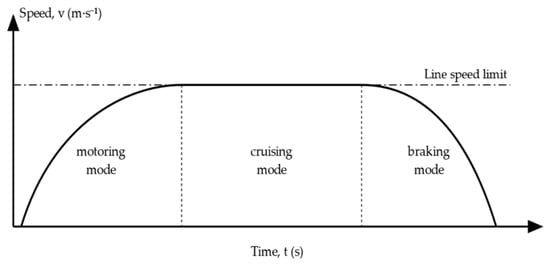
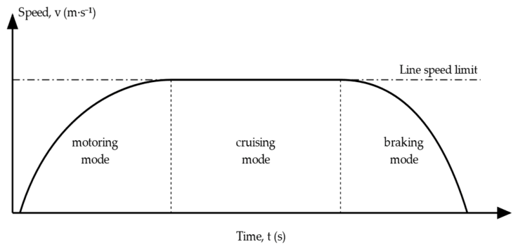
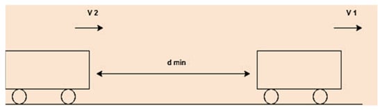
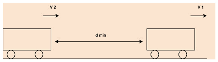
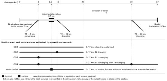
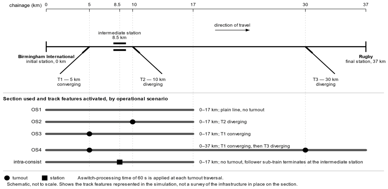
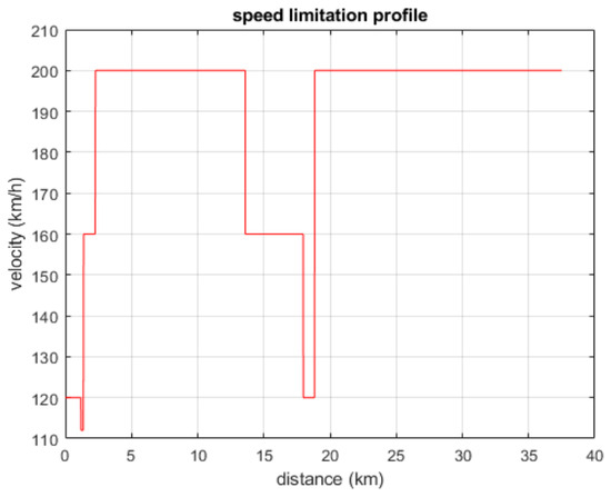
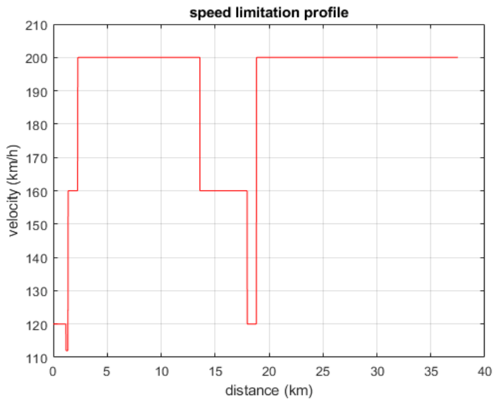
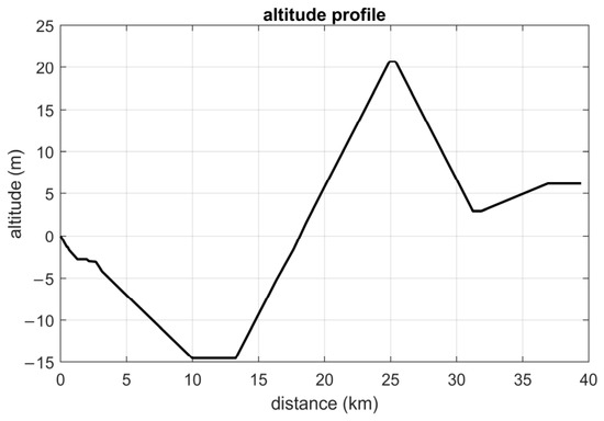
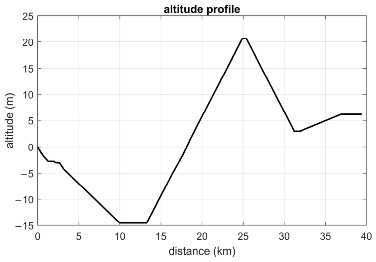
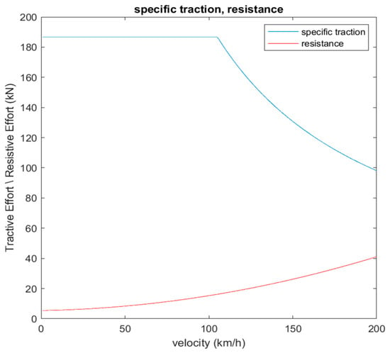
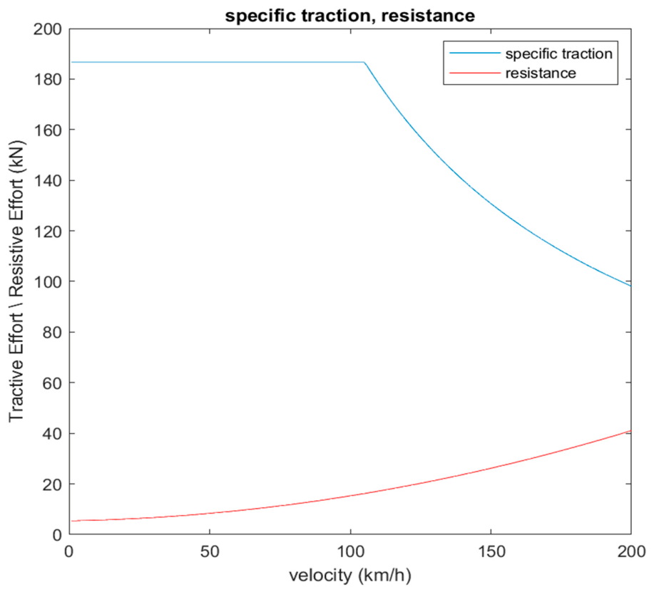
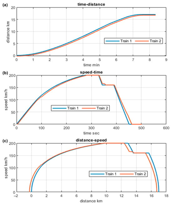
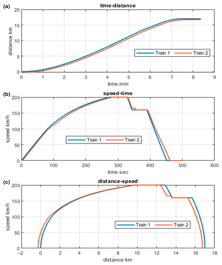
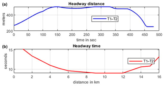
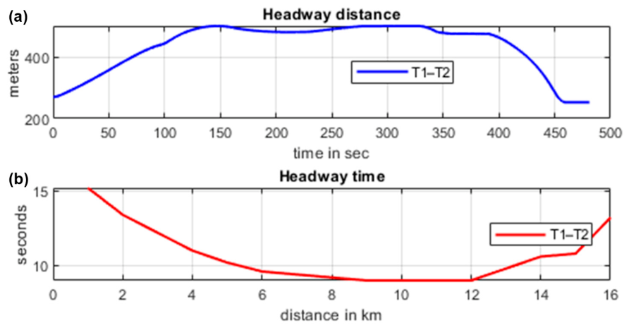
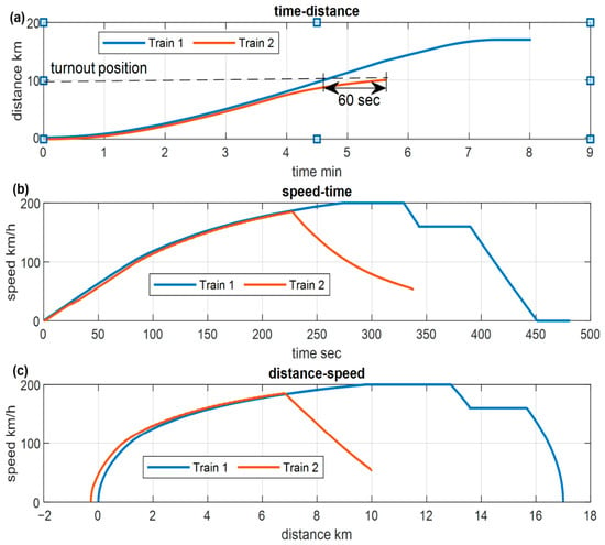
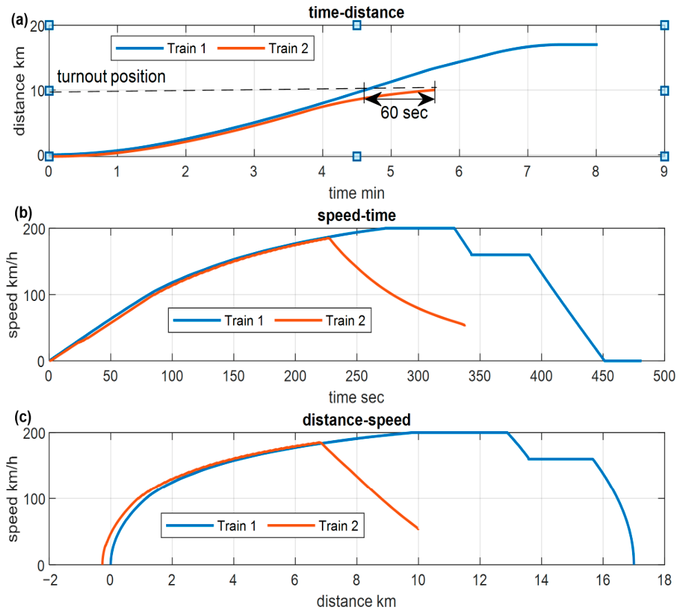
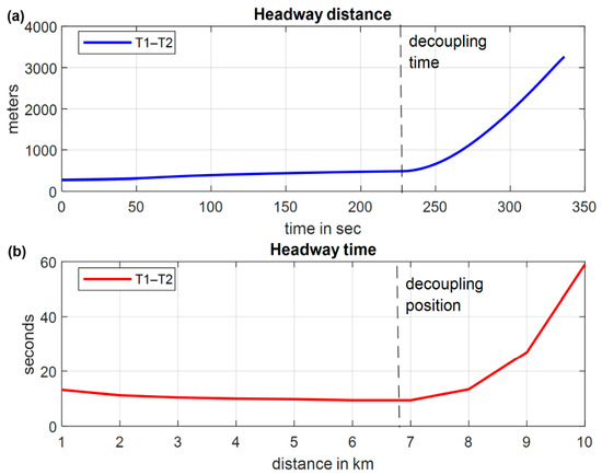
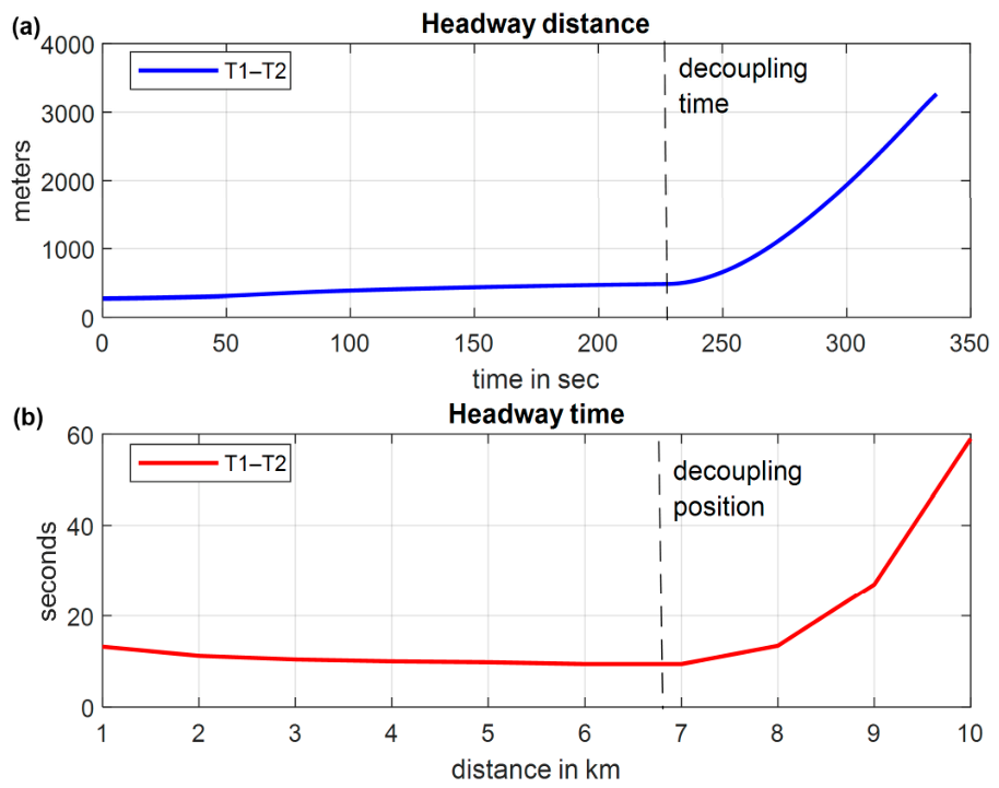
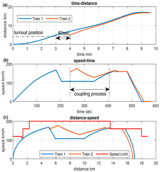
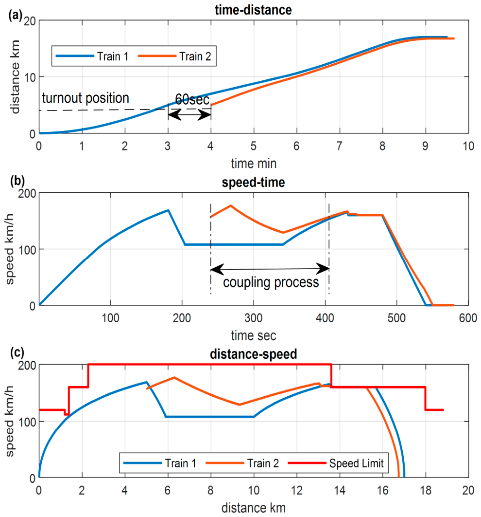
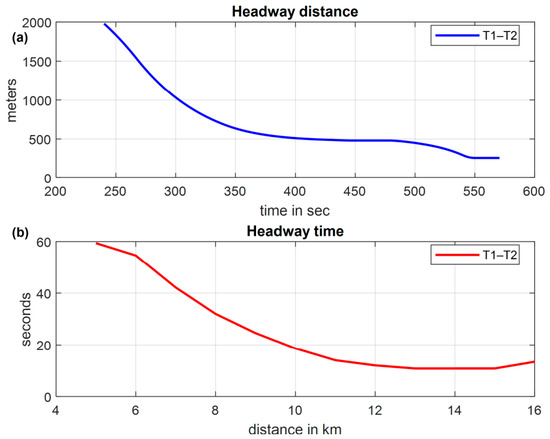
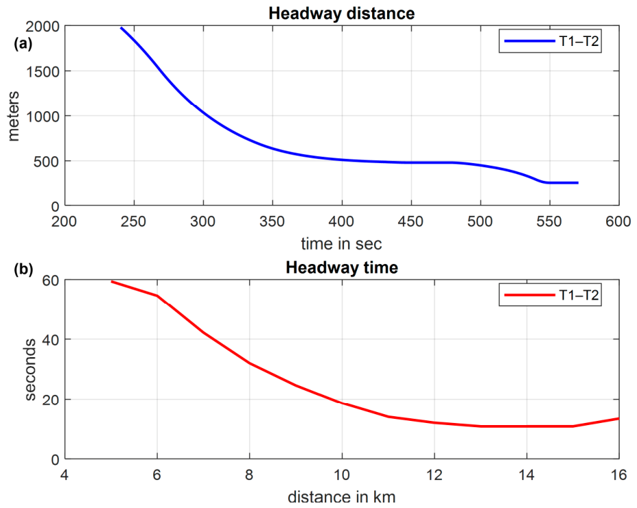
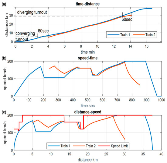
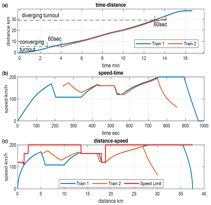
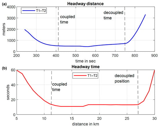
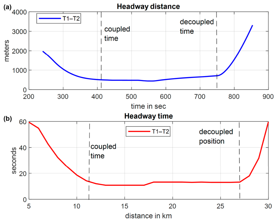
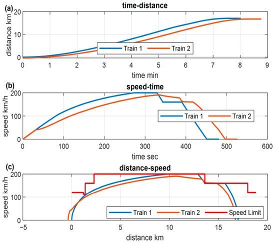
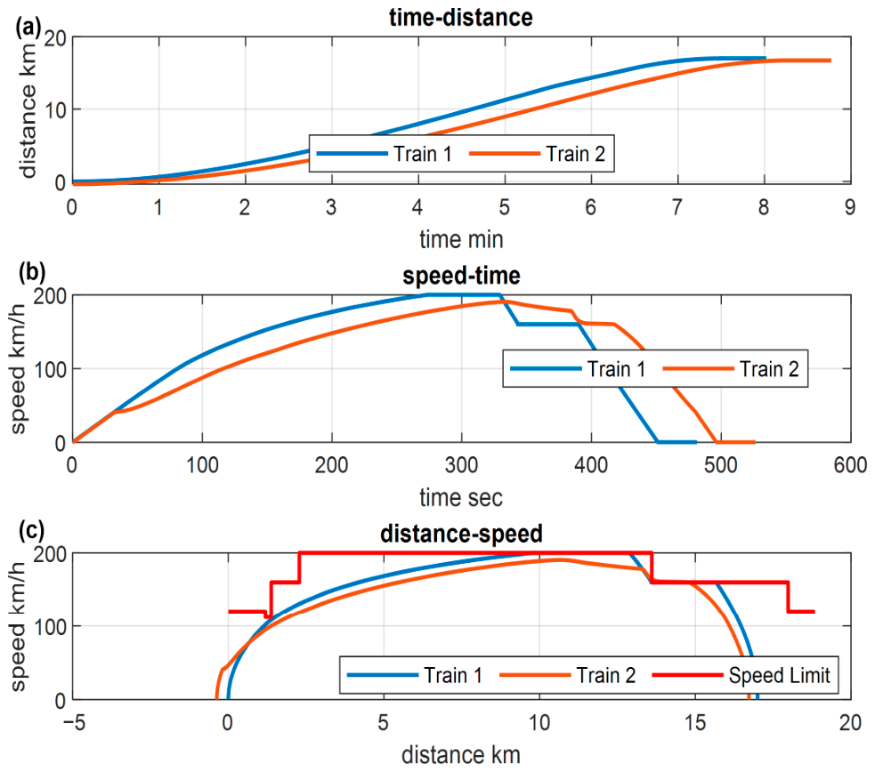
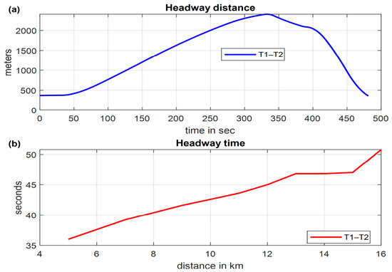
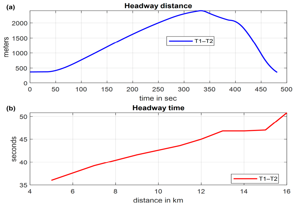
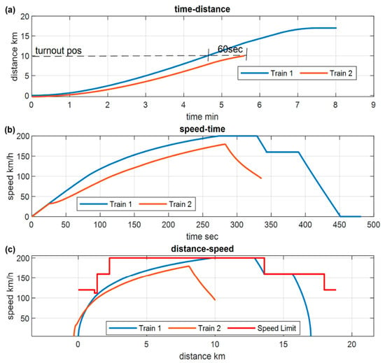
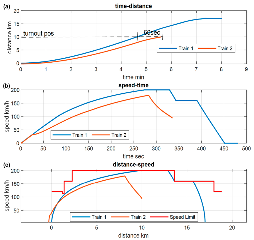
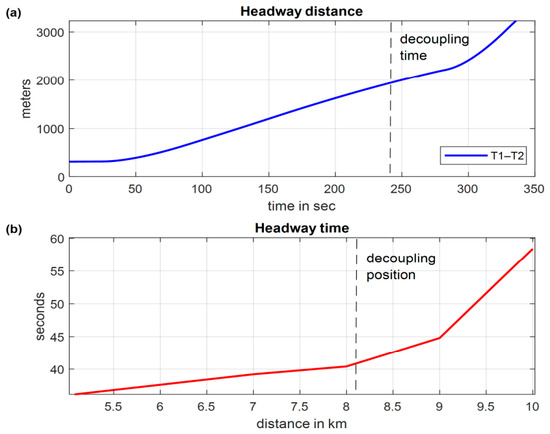
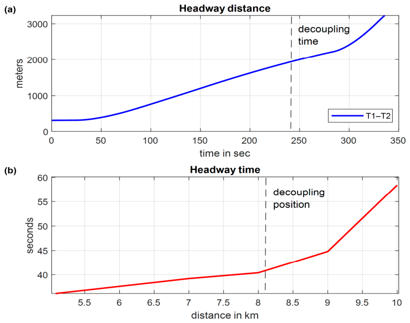
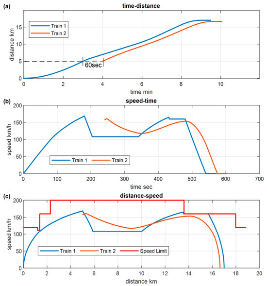
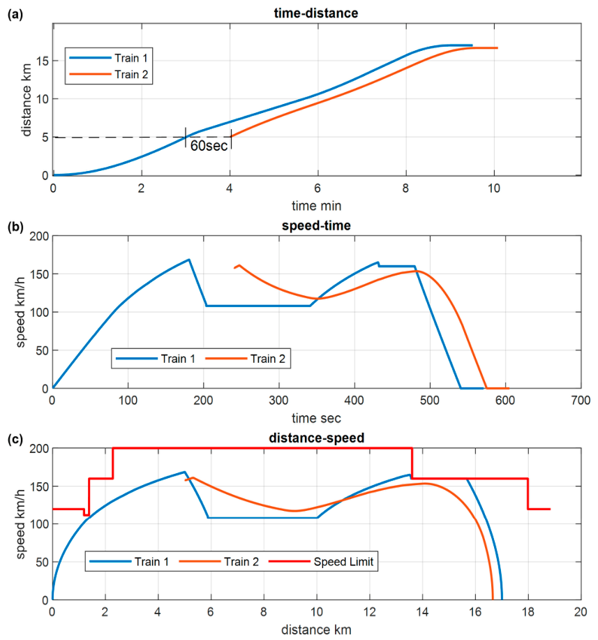
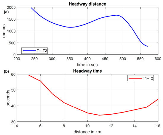
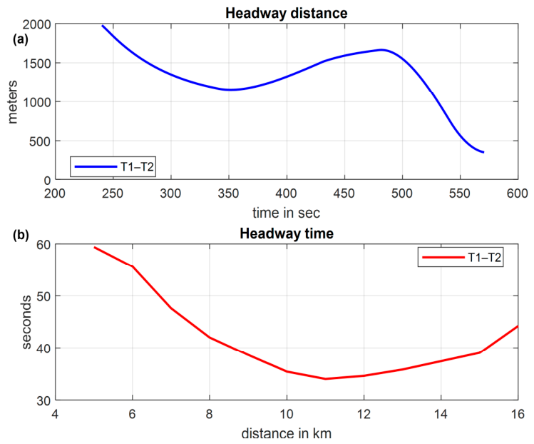
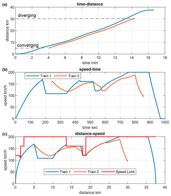
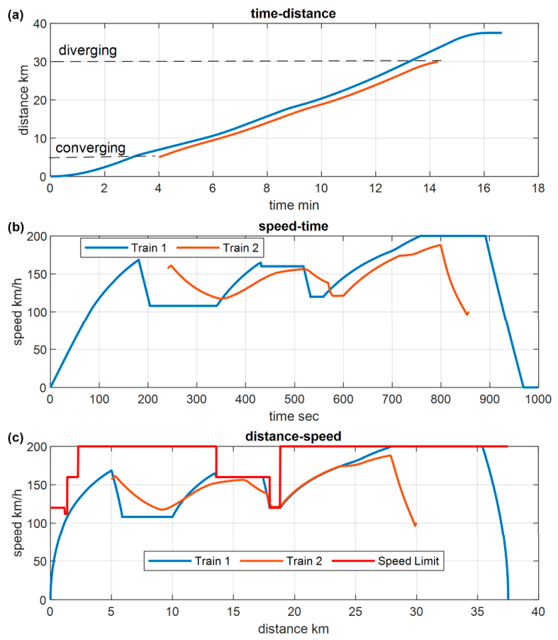
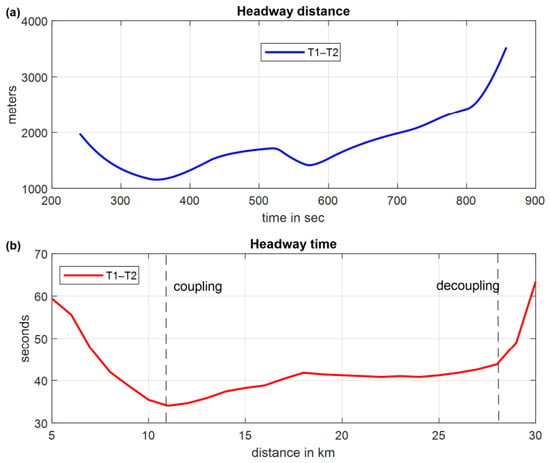
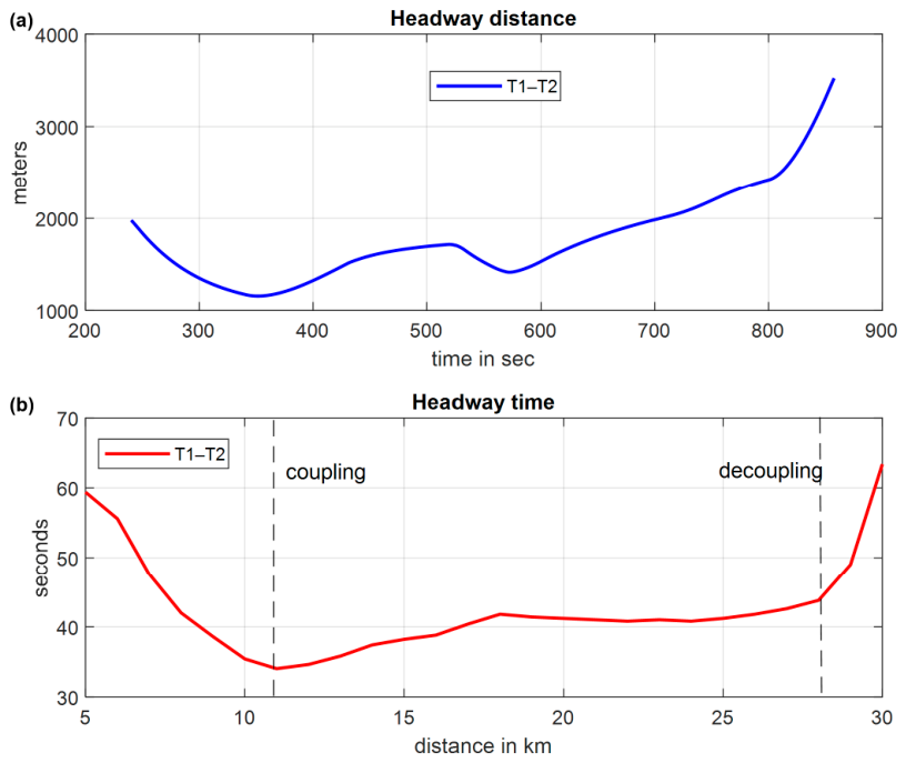
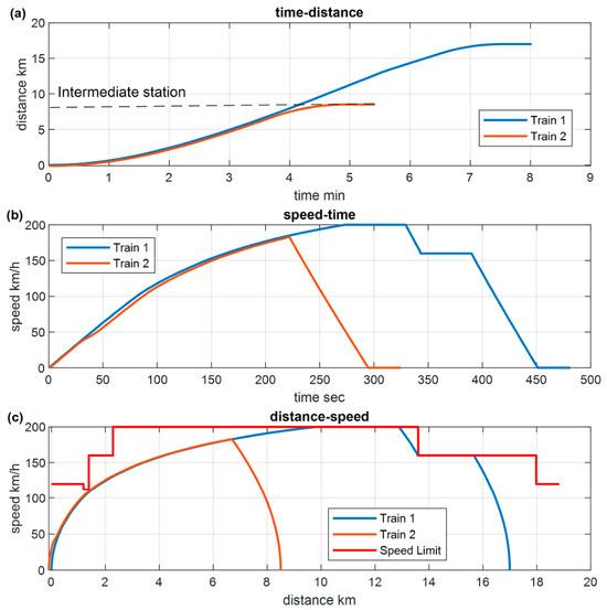
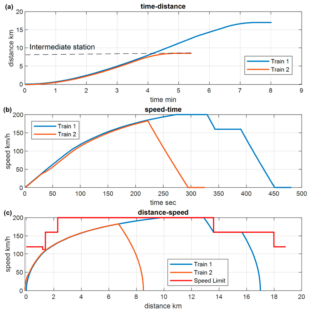
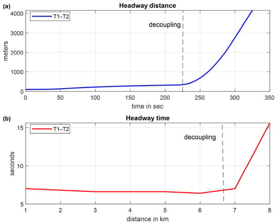
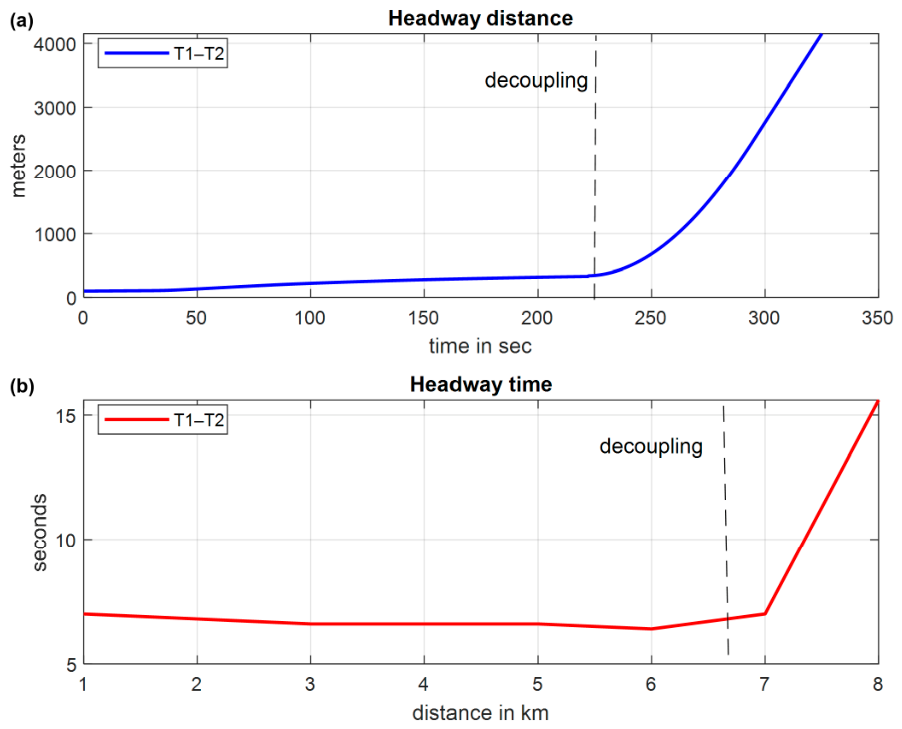
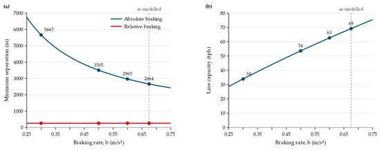
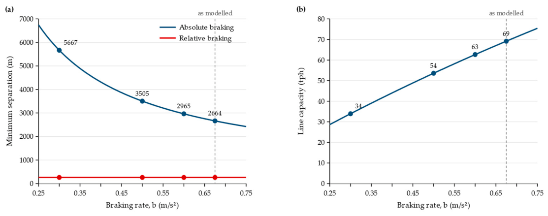

Disclaimer/Publisher’s Note: The statements, opinions and data contained in all publications are solely those of the individual author(s) and contributor(s) and not of MDPI and/or the editor(s). MDPI and/or the editor(s) disclaim responsibility for any injury to people or property resulting from any ideas, methods, instructions or products referred to in the content. |
© 2026 by the authors. Published by MDPI on behalf of the International Institute of Knowledge Innovation and Invention. Licensee MDPI, Basel, Switzerland. This article is an open access article distributed under the terms and conditions of the Creative Commons Attribution (CC BY) license.