


Abstract
The text deals with Milanković’s Mathematical–Astronomical Theory of Ice Ages and its connection with Serbian loess. Here it is recalled, put into the context of the people who collaborated with Milanković during his work (W. Köppen, A. Wegener, V. Mišković, W. Jardetzky, D. Mitrinović, and S. Fempl), and it points to its 50th anniversary of verification in the journal Science. Then, the Theory is compared with magnetic susceptibility (MS) profiles of two Serbian loess–paleosol sequences (Mošorin and Stari Slankamen) by (i) showing side-by-side the Milanković’s Insolation Curves and the MS Curves over the last 600,000 years and (ii) discussing the relation of the MS spectral components and the orbital (eccentricity, obliquity, and precession) and terrestrial (solar constant and albedo) forcing of Milankovic’sTheory. In addition to the similarities between Milanković’s Insolation Curves and the MS Curves, there are discrepancies, the causes of which are analyzed in detail. The text ends with a biographical section on Milanković’s voyages down the Danube and the StariSlankamen profile, where in the layers of loess there are visual traces of the change in glacial (Ice Ages), cold intervals and interglacial (Inter Ice Ages), warm intervals in the geological history of the Earth. These traces match relatively well with Milanković’s Insolation Curves, which he could not have known during his many passes. In the conclusion, suggestions are given on how to reduce the discrepancies between Milanković’s Insolation Curves and the MS Curves and thereby improve paleoclimatological research.
1. Introduction
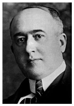
World famous contributions to climatology and the Mathematical–Astronomical Theory of Ice Ages were those of Milutin Milanković (Dalj, (Austro-Hungarian), 1879—Belgrade, 1958), Figure 1.
Figure 1.
Milutin Milanković (1879–1958) was the creator of the Mathematical–Astronomical Theory of Ice Ages [1], or “Milankovitch theory”, as stated in [2] (The “Milankovitch theory” was confirmed 1976, 35 years after its publication (1941) and 18 years after Milanković’s death (1958), and this year is half a century since its verification, which should be considered a kind of jubilee). In this paper the presence of orbital components in deep-sea cores was established at times predicted by the Theory, which was also his theory verification based on sampling and measurements. The Theory explained in a completely scientific way, without any non-scientific postulates, the change in glacial (Ice Ages), cold intervals and interglacial (Inter Ice Ages), warm intervals in the geological history of the Earth in the last 600,000 years.
A civil engineer by training, Milutin Milanković completed the Polytechnic School in Vienna, which was then one of the most prestigious engineering schools in the world. In Vienna, in 1904, he earned a doctorate in civil engineering on the topic of concrete structures, and afterwards he worked as a construction engineer. In 1909, he left his prosperous career in Vienna to pursue a career as a university professor in Belgrade, teaching rational mechanics, Celestial Mechanics, and Theoretical Physics. Later, during the 1926/27 school year, he became the Dean of Faculty for the Department of Philosophy [3]. For a short time in 1950, he was also the Head of the Astronomical Observatory in Belgrade. Milutin Milanković was a full member of the Serbian Academy Sciences and Arts, and also a corresponding member of the Yugoslav Academy of Sciences and Arts in Zagreb (Croatia).
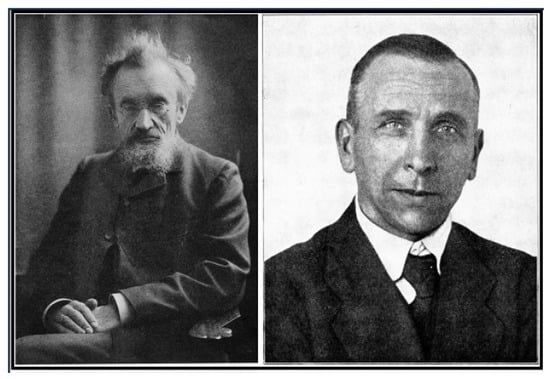
Milutin Milanković is one of the founders of modern climatology and mathematical climate modeling [3]. He developed his Theory on certain ideas of Wladimir Köppen (Sankt Petersburg, 1846—Graz, 1940) and Alfred Wegener (Berlin, 1880—Greenland, 1930), Figure 2. These are ideas related to the climate of the Earth’s past presented in a famous book in German “Die Klimate der geologischenVorzeit” [4]. In addition, their cooperation took place through extensive correspondence and personal contacts [5].
Figure 2.
Wladimir Köppen (1846–1940), left, was a geographer, meteorologist, and climatologist. Alfred Wegener (1880–1930), right, was a climatologist, geologist, geophysicist, meteorologist, and polar researcher. Both of them helped Milutin Milanković with their useful advice for creating the Theory of Ice Ages.
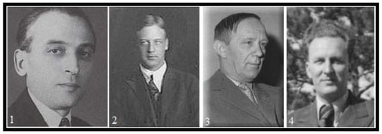
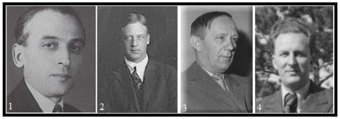
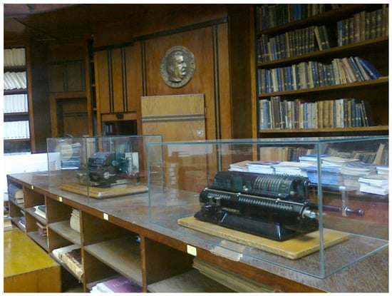
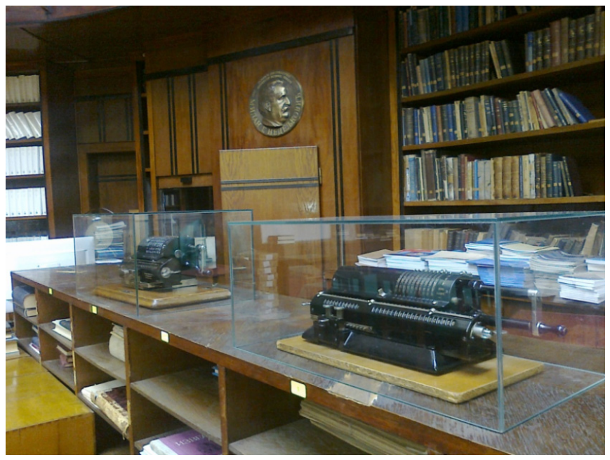
Also, Milanković had great help in creating the Mathematical–Astronomical Theory of Ice Ages from two astronomers: Vojislav Mišković (Fužine (Austro-Hungarian), 1892—Belgrade, 1976), the long-time Director of the Astronomical Observatory in Belgrade [6], and Wenceslas Jardetzky (Odessa, 1896—Elkins, West Virginia (USA), 1962), Milanković’s PhD student, thereafter a professor at the University of Belgrade and later a professor at Columbia University in New York [7], Figure 3 (1 and 2); they made contributions to the astronomical postulates of the Theory of Ice Ages; and two mathematicians Dragoslav Mitrinović (Smederevo (Serbia), 1908–Belgrade, 1995) and StanimirFempl (Zemun (Austro-Hungarian), 1903–Belgrade, 1985), both professors of mathematics at the University of Belgrade, Figure 3 (3 and 4); they made contributions in the mathematical calculations of astronomical and other equations using the then contemporary pinwheel desktop mechanical calculators, Figure 4.
Figure 3.
(1) Vojislav Mišković (1892–1976), astronomer as the long-time Director of the Astronomical Observatory in Belgrade, (2) Wenceslas Jardetzky (1896–1962), astronomer and professor of the university, (3) Dragoslav Mitrinović (1908–1995), mathematician and professor of the university, and (4) Stanimir Fempl (1903–1985), mathematician and professor of the university.
Figure 4.
On display at the library of the Astronomical Observatory in Belgrade are two pinwheel desktop mechanical calculators: Swedish Original Odhner Göteborg (left) and German “Brunsviga” System Trinks (right) on which it calculated Mathematical–Astronomical Theory of Ice Ages of Milutin Milanković’s, (Photo: N. Janc, June 2015).
2. Publishing
Milanković developed a consistent Mathematical–Astronomical Theory of the Ice Ages (paleoclimate change) in many works and through very frequent written correspondence with his collaborators mentioned above. Many letters from this correspondence have been preserved. Their publication in the original form is ongoing [5,6,7].
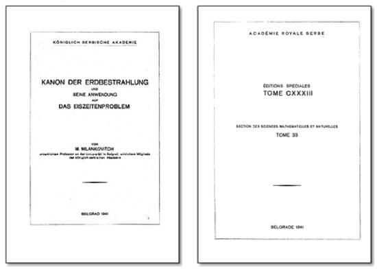
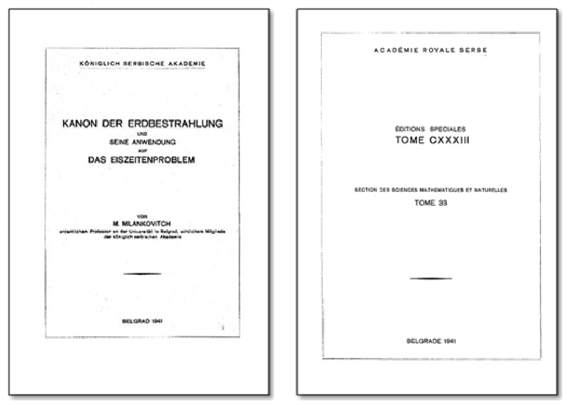
From the published papers, we will single out two papers according to the chronology of their appearance. First is “Mathematical Theory of Thermal Phenomena Caused by Solar Radiation”, or the original title in French “Théorie Mathématique des Phénomènes Thermiques Produits par la Radiation Solaire” [8], which was in the middle of the research period. In the second paper, the final version of the Theory of Ice Ages was presented, and it was in the form of a book “The Canon of Earth’s Insolation and Its Application to the Problem of Ice Ages” or “The Canon of Insolation” for short or only “CANON” while the original German title was “Kanon der Erdbestrahlung und seine Anwendung auf das Eiszeitenproblem” [1,9], Figure 5.
Figure 5.
The title page (left, on German) and next page (right, on French) of Milankovitch’sbook “Kanon der Erdbestrahlung und seine Anwendung auf das Eiszeitenproblem” (“The Canon of Earth’s Insolation and Its Application to the Problem of Ice Ages” [1] (Commonly translated into English as “The Canon of Insolation and the Ice-age Problem”, while in [2] it is cited as “M. Milankovitch, K. Serb. Akad. Beogr. Spec. Publ. 132 (1941) (translated by the Israel Program for Scientific Translations, Jerusalem, 1969)”).
According to Milanković’s Theory, climate changes on the planet Earth in long periods depend on Insolation or on the amount of heat that the Earth receives from the Sun. This amount of heat does not depend on the sun as the main and constant source of heat, but depends on the movement of the Earth, which periodically changes its exposure to the sun over time. This changes the amount of heat received by the Earth, which represents the so-called astronomical influence on the climate, or astronomical forcing of the climate, which is the basis of Milanković’s Theory of Ice Ages.
3. Results and General Verifications
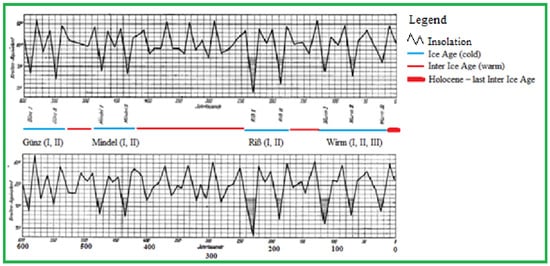
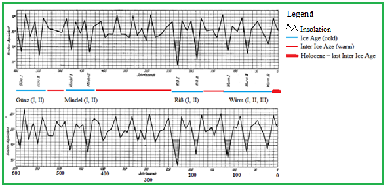
The main results of the Mathematical–Astronomical Theory of Ice Ages are Milanković’s Insolation Curves (Insolation), Figure 6. Here, the horizontal axis is time over the last 600,000 years, and the vertical axis is the amount of energy the Earth receives from the Sun. Insolation oscillates and shows haveminima and maxima values. During the minimum, temperatures on the Earth’s surface decrease and cold geological periods occur known as Ice Ages (Günz (I, II), Mindel (I, II), Riß (I, II), and Würm (I, II, III)), while during the maximum, temperatures rise and warm geological periods occur known as Inter Ice Ages, and previous Ice Ages disappear.
Figure 6.
Milanković’s Insolation Curves (Insolation) that show amplitudes of secular changes in the summer Insolation at the 65° N (vertical axis) during the last 600,000 years (horizontal axis), (Figure 48 in [1]), modified with the Legend where blue, red, and thick red lines show the approximate duration of Ice Ages, Inter Ice Ages, and the Holocene, respectively.
Milanković’s work only gained world-wide significance posthumously, when his findings were clearly scientifically validated first in the paper of [2], and later confirmed in other studies [10,11]. Milanković’s Theory eventually became known to the general public thanks to the popular book “Ice Ages—Solving the Mystery” by Imbrie and Imbrie [12].
The Theory suggests that orbital forcing operates in cycles of approximately 20,000 to 400,000 years. It is largely determined by the geometry of the Earth’s motion around the Sun, i.e., the so-called astronomical factors. Milanković explained this exactly by writing out and solving mathematical equations of celestial and rational mechanics, countering various descriptive speculations about the paleoclimate that were popular and widespread at that time. Scientific evidence of the correctness of Milanković’s Theory was found all over the world and is still being found in geological, oceanographic, and other samples. Also, his ideas were confirmed by additional theoretical research [13,14].
4. Verification in Serbia
4.1. Study Area and Loess Profiles
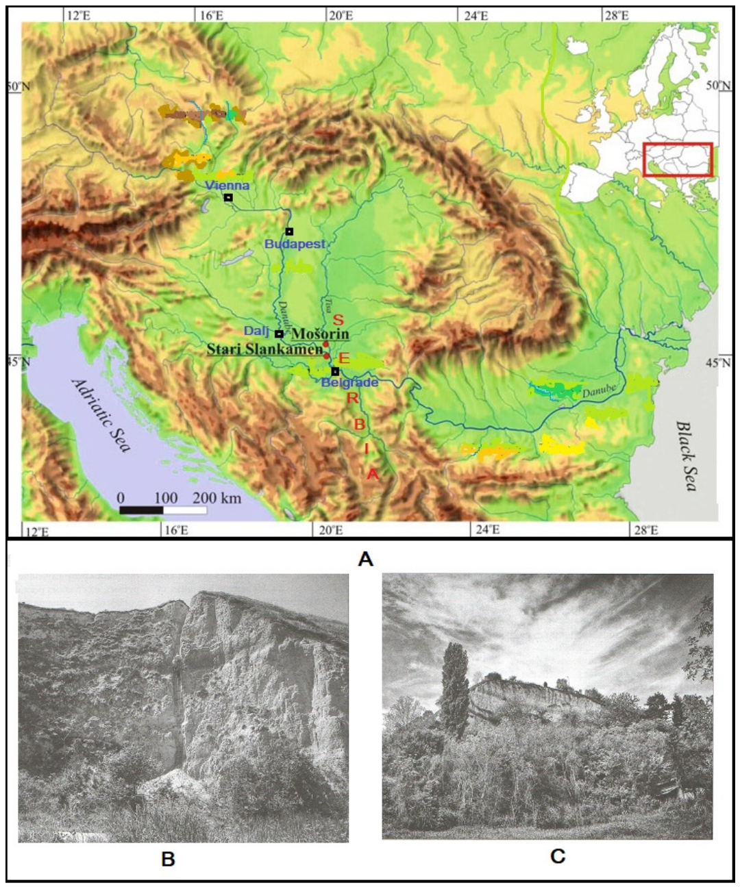
The Republic of Serbia is a European country located in the middle latitudes (~45° N), Figure 7A. The southern part of its territory occupies the space on the Balkan Peninsula, and the northern part is located in the S-E part of the Pannonian Plain, i.e., the middle Danube. This geographical area is rich in loess–paleosol sediments, which have been well explored in the last 7–8 decades through many papers [15,16,17,18,19,20,21,22,23,24,25,26,27,28,29,30,31,32,33,34,35,36,37,38,39,40,41,42,43,44,45,46,47,48,49,50,51].
The main goal of this research is the comparison of Milanković’s Insolation Curves with MS Curves obtained from Serbian loess. In order to do this in the correct way, it is very necessary that the time series of both values be of sufficient continuous length, that is, at least 600,000 years, for which period Milanković’s Insolation Curves were calculated, Figure 6. The previous requirements are met by two loess profiles: Mošorin [52] and Stari Slankamen [53], whose locations and typical photos are shown in Figure 7.
Figure 7.
(A) The locations of the loess profiles Mošorin and Stari Slankamen in Republic of Serbia, and the locations of the 4 cities: Belgrade, Dalj, Budapest, and Vienna, where Milutin Milanković spent most of his life and where he built the Mathematical–Astronomical Theory of Ice Ages ([54], modified). The red frame indicates the study area on the map of Europe (upper right corner). (B,C) Typical visual views of both profiles Mošorin and Stari Slankamen [55].
4.2. Method
The ideal way to verify a scientific theory would be to compare the same physical values obtained from the theory and by measurement. In this case, the theoretical values are Milanković’s Insolation Curves. Since the same value as measured does not exist, the measured values of the magnetic susceptibility (MS) from Serbian loess samples will be used as an equivalent quantity for comparison. For this, the hypothesis that there is an interaction between Solar radiation (Insolation) and MS of Serbian loess will be used because there are some scientific indications of this, but there is no solid experimental evidence (see Supplementary Material). This hypothesis is supported by the fact that there have been many studies on increased MS formation in pedogenesis, e.g., [56,57,58,59].
In the first approach, Milanković’s Insolation Curves (Insolation data) will be compared with the measured values of MS Curves (MS data).
In the second approach, the spectral components of MS (MS spectrum) will be compared with the spectral components of Milanković’s Insolation Curves (Insolation spectrum).
5. Insolation and MS Data
For the purposes of this research, the values of Insolation and MS will be used exclusively from the papers [1] and [54], respectively.
For Insolation, we will use: (i) its original graphic appearance (Figure 48 in [1]), already shown here in Figure 6, and (ii) mathematical–physical conditions on how to obtain Insolation in [1], using three orbital/astronomical forcing (eccentricity, obliquity, and precessionas known components of the Insolation spectrum) and two terrestrial/parametric forcing (solar constant and albedo), with which Milanković defined the Theory of Ice Ages.
For MS, two original graphs will be used. The first graph is (iii) Figure 6 from paper [54], here it is Figure 8, where the time series of measured MS values is shown, from which, using Figure 6, Figure 9 is obtained. The second graph is (iv) Figure 7 from paper [54], here it is Figure 10, where the MS spectrum is shown, i.e., the frequency distribution of climatic forcing recorded in MS. All of this relates to the period of the last 1,000,000 years at the Mošorin and Stari Slankamen loess profiles.
Figure 8.
Smoothed MS record/data (horizontal axis) of the composite loess–paleosol sequence of the Mošorin and Stari Slankamen loess profiles over the last approximately 1,000,000 years (vertical axis), (Figure 6 in [54]), which is unmodified except for the added blue rectangle separating the last 600,000 years for direct comparison with the same period in Figure 6 here. In the middle between the vertical axis and the chart, there are nomenclature marks, in this case only the soil layers with abbreviated meaning: V—Vojvodina, S—Soil, and a number, as the ordinal number of the layer from top to bottom, so on the chart there are marks V S1–V S9 or a total of 9 soil layers designated as (paleo) soil, and between them there are loess layers that would be labeled …V L2–V L8…, respectively. The meanings of other symbols and terms can be found in the original paper [54].
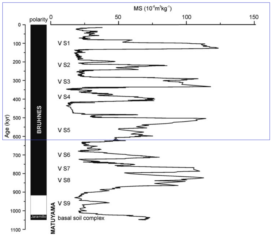
As can be seen in Figure 8, the MS values vary by about an order of magnitude, (12–124) × 10–8 m3 kg–1. The minimum MS values are about 12 × 10–8 m3 kg–1 in two cases, around 350,000 years ago and around 440,000 years ago, while the maximum MS value is around 124 × 10–8 m3 kg–1 around 130,000 years ago.
Furthermore, a periodic change in high and low MS values is observed. There are 10 such shifts with high MS values, of which nine are designated nomenclature as V S1–V S9. Between them there is the same number of low MS values that are not marked, which would be written as V L1–V L9. More details about all this can be found in the aforementioned paper by [54] and other previously mentioned papers, so it will not be discussed anymore.
6. Comparison of Insolation and MS Graphs
Based on the hypothesis on the interaction of Insolation and MS (see Supplementary Materials) that high values of MS mean increased Insolation, and low values of MS mean reduced Insolation, both values MS and Insolation will be compared graphically (first approach). Now we will directly compare the graphs of Milanković’s Insolation Curves in Figure 6 with the graph-measured values of MS in Figure 8. It seems that the visual comparison, which will be sufficient for this occasion, can best be done if we bring both graphs to the same scale, along the same oriented vertical and horizontal coordinate axes and place the second graph (MS) vertically below the first (Insolation), Figure 9.
Figure 9.
(a) Milanković’s Insolation Curves same as Figure 6; (b) smoothed MS record of the Mošorin and Stari Slankamen same as Figure 8 rotated clockwise by 90°; and (c) view of just the MS from the blue rectangle in panel (b), which homogeneously stretched along the time axis to adjust for direct comparison with Milanković’s Insolation Curves in panel (a), where horizontal blue and red lines indicate estimated mean MS values for intervals covered by lines, with low MS values (MS1, MS3, MS5, and MS7) marked in blue and high MS values (MS2, MS4, and MS6) marked in red and connected by vertical lines to the Ice Age and Inter Ice Age intervals (below) transferred from panel (a).
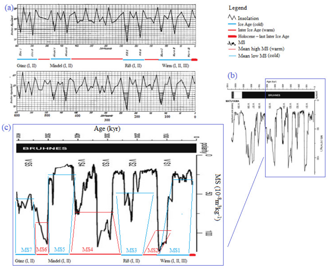
It should be noted that in Figure 9c with MS1, MS3, MS5, and MS7 are marked paleo intervals of low average values of MS (blue), when it is colder on the Earth’s surface, and with MS2, MS4, and MS6 are marked intervals of high MS values (red), when it is warmer on the Earth’s surface. Further, it can be seen that in the last 600,000 years there were a total of seven intervals, starting from the closest cold one, MS1, then the closest warm one, MS2, etc., until the last cold one, MS7.
We observe that the cold and warm MS intervals alternate in the same way as the cold and warm intervals obtained from Milanković’s Insolation Curves alternate, that is, as the Ice Age and the Inter Ice Age alternate. At the same time, on the timeline the cold MS intervals coincide with Ice Ages and the warm MS intervals coincide with Inter Ice Ages, which can all be seen on the correspondingly placed panels (a), above, and (b), below, both in Figure 9, respectively.
6.1. Verification by Curves
Insolation and MS Curves have similarities and differences during the 600,000 years. Matching the number and sequence of their intervals with high and low values supports the existence of a similarity. This may lend weight to the view that Milanković’s Theory is not in conflict with the MS data obtained from Serbian loess.
At the same time, there are differences between Insolation and MS, which are not negligible. For example, the widths of the equivalent warm and cool intervals of Insolation and MS are not the same. Furthermore, the degree of smoothness of the curves differs significantly. Insolation is very smooth over long intervals, whereas the MS Curve is highly jagged/peaky. This may not be the most important factor but it should not be overlooked. Part of the explanation of the differences will be further discussed in the next Chapter using the second approach, comparing Insolation and MS in phase space.
6.2. Advantages and Disadvantages
The graphical comparison between Insolation and MS has advantages and disadvantages.
The advantage of the method is that similarities and differences between Insolation and MS can be visually observed. It would be good if the visualization could be demonstrated quantitatively, but unfortunately the large difference in the number of degrees of freedom of the data (see Section 7.6) and the lack of original data in digital form make it impossible to apply good statistics for comparison. In fact, statistics could be made, but the obtained results would have more numerical than scientific value, which would create additional unnecessary errors. Also, the possibility of reconstructing the original data remains as only a principled option, which is impractical in practice.
The disadvantage of the method is that it does not show the physical processes that created the Insolation and MS values. True, these physical processes are known for Insolation, because they are part of the postulates of Milanković’s Theory, but they are not known for MS. The discussion about this follows in the next Chapter within the application of the spectral comparison method (second approach).
Two remarks remain. The first, the present day Inter Ice Age (Holocene) was not taken into consideration because its MS data were not available. The second, there are also some discrepancies between Insolation Theory and MS measurements, which will be discussed in the next Chapter.
7. Comparison of Insolation and MS Spectra
The spectral comparison (second approach) is more suitable when it is necessary to determine differences in spectral components, that is, the physical processes (forcing) involved in the generation of climate variability. Every physical process should be represented by at least one spectral component. Also, noises have their own spectral components, which encourage “artificial” forcing caused by errors in sampling, measurements, calculations, and flaws of methods.
Here, the spectral comparison will have two roles: (i) for additional and more reliable verification of Milanković’s Theory in relation to Serbian loess and (ii) to explain the discrepancies in the similarity of Insolation and MS discussed in the previous Chapter. This will be carried out through a discussion of the eight cases that follow.
7.1. Case 1—Spectral Components of Insolation
Milankovitch’s theory is based on the geometry of the Earth’s motion around the Sun, with a limited number of climate forcing factors. Three factors are movements of the Earth (eccentricity, obliquity, and precession), one is the solar constant, and last is the effect of snow cover on albedo, which is the only terrestrial forcing (totaling five factors).
Milankovic’s Theory does not take into account other forcings on climate. These are other movements of the Earth and, if not all, at least the most important terrestrial (meteorological, hydrological, geological, other physical, chemical, and biological) processes. It should be noted here that the Earth’s atmosphere and its climate are considered one of the most complex inanimate physical systems in the universe [60]. So, any interpretation of the climate, whether theoretical or practical, is a very complex problem because it is in the domain of all natural sciences.
7.2. Case 2—Spectral Components of MS
Contrary to the calculated values of Milanković Insolation obtained only by considering the five forcing factors, the measured values of MS from field loess samples were formed under the influence of all existing forcings, both astronomical and terrestrial, not only geological–atmospheric, but also biological. All these processes will not be listed here. Even if there was such an intention, it would be a problem to count them all, so it is safe to say that they are uncountable. If we add to this their property of non-linearity [61,62], which means that in mutual interactions they create new processes [63,64], any attempt to enumerate the total number of processes that have affected MS is almost impossible. It is so in theory, but in practice it is different. Their influence on the climate is determined by spatial and temporal scales. Thus, their number on the given scale is finite. In addition to these, there are also processes caused by noise arising from errors in sampling, measurement, and calculation.
In addition to all the problems related to the identification of the processes that affect MS, it is possible to establish a lot. To begin, let us look at Figure 10, which shows the spectrum of the smoothed MS record of the composite loess–paleosol sequence of Mošorin and Stari Slankamen in the last approximately 1,000,000 years (Figure 7 in [54], modified).
On the spectrum, 24–25 peaks can be counted, each representing the influence of some factor on the climate, known as forcing on the climate. In the paper of [64], eight peaks are recognized, marked with numbers. Seven of these peaks are recognized as Milanković cycles: (i) forcing by eccentricity with periods from 256 kyr and 97 kyr; (ii) forcing by obliquity with periods from 38 kyr and 35 kyr; and (iii) forcing by orbital with periods from 24 kyr, 22 kyr, and 19 kyr. It is surprising that the remaining eighth peak of 66 kyr was also found in Chinese loess samples [65].
Figure 10.
Spectral analysis results using the tuned MS time series record of the Mošorin and Stari Slankamen composite loess–paleosol sequence for the past 1,000,000 years. The relative MS amplitudes (vertical axis) are shown as a function of frequencies/periods (horizontal axis). The numbers above the peaks represent dominant cycles/periods in units of one thousand years (kyr), while unknown (unidentified) peaks are marked in red lines (Figure 7 in [54], modified).
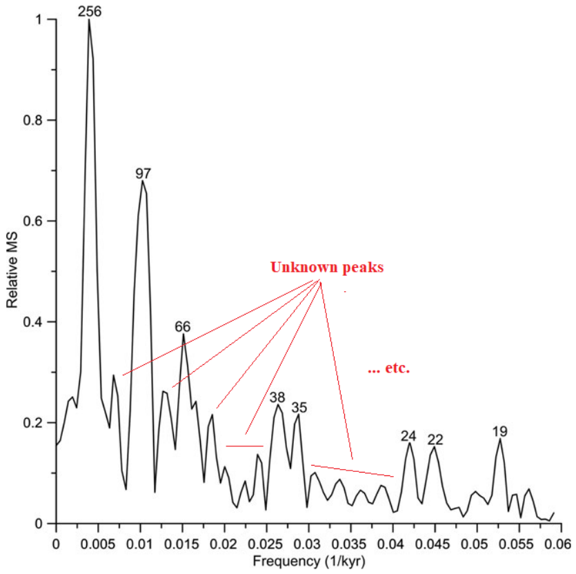
Since a peak of 66 kyr is not linked to the cause, it can be considered as unknown forcing. It remains to be determined whether it stems from unknown astronomical forcing, terrestrial forcing (atmospheric circulation [66], oceanic processes [67], geological changes, and biological–anthropogenic factors), or is the product of non-linear interactions between these factors (see Section 7.5).
7.3. Case 3—Unknown Climate Forcings
The remaining 16–17 (unknown) peaks were not recognized, Figure 10. They represent some currently unknown impacts on the paleoclimate. That is why it is necessary to identify them, if only like the eighth peak (66 kyr). To begin with, one should find other such periods in the spectra of other loess profiles, for example, in Chinese loess, and then proceed to identify their causes.
The difference between Milanković’s Insolation and the MS is that the first one was obtained on the basis of only five forcing factors (eccentricity, obliquity, precession, solar constant, and albedo), and the second one on the basis of 24–25 forcings. In order to reduce the differences, other forcings should be added in the first case, and unknown forcings should be recognized in the second case.
The aim of this text is not to explore these unknown peaks in greater detail, but merely to point out a possible direction for further research. These currently unexplained peaks are indicators of climate signals that require a causal interpretation.
7.4. Case 4—Verification by Spectra
At first glance, it seems that Milanković’s Theory has no confirmation in the MS spectrum, because it has only five forcings, and the MS spectrum has 24–25 forcings. However, the opposite is true. Milankoć’s Theory has a good foothold in the MS spectrum, since all three astronomical forcings (eccentricity, obliquity, and precession) are found in it. This kind of argumentation in favor of Milanković’s Theory is completely analogous to its verification in [2]. The Theory was accepted after the discovery of orbital components in deep-sea sediments.
Astronomical forcings are the most important because they had a dominant influence in the creation of the Ice Ages, which Milanković showed with his Theory, at least in the case of Serbian loess. Other (unknown) forcings (16–17 peaks) are not unimportant, but for the time scale of the Ice Ages they seem to be of lesser importance. This does not mean that they should be left uninvestigated.
7.5. Case 5—Non-Linear Phenomena
This is an opportunity to mention two interesting non-linear phenomena regarding atmospheric or climatic behavior that have been demonstrated in numerical experiments.
The first phenomenon—change in parameters. The paper [62] shows that a very small change in gravity or the Earth’s radius leads to very large changes in wave processes. Analogously, it seems that small changes in other parameters can lead to significant changes in climate behavior.
The second phenomenon—initial state. The paper [64] demonstrates that during a non-linear numerical simulation of the atmosphere, if the initial excitation comprises only three wave components or cycles (the minimum number required for non-linear interaction), a larger number of new cycles (14–15 in this case) emerge over time. In numerical experiments this lasts until the dissipation of the system, but in nature it is eternal or until some great catastrophe in nature. If the system is restored, the process continues.
Both phenomena are properties of non-linear physical systems such as the atmosphere and probably also apply to paleoclimatic time scales, for which there seems to be no information. On the other hand, both phenomena are easier to monitor in numerical experiments than in nature, which does not have a rapid change in parameters or a clearly defined initial state.
7.6. Case 6—Resolution
In the case of Milanković’s Insolation Curves, we see from Figure 6 that the time resolution has 10 same intervals on every 100,000 years, or a total of only 60 grid point intervals to display the Insolation during the 600,000 years for which Milanković calculated the Insolation. Insolation was calculated, more precisely shown in Figure 6, every 10,000 years, which is a very small resolution for modern times. For us, the present people, it is the duration of the Holocene, and in that one interval we can place all human cultures and civilizations from the beginning to the present day. Again, for the entire paleo period in which Ice Ages were identified, this is a large enough resolution because it can encompass the periods of all the movements that Milanković took into account when he created his “Ice” Theory.
Now we will calculate the number of grid point intervals on the MS time scale. Otherwise, loess conversions from depth scale to time scale are not simple. Loess does not have linear homogeneity, so it happens that thinner layers of loess were formed in longer time intervals than thicker layers, as well as vice versa [68], which will not be discussed further here.
It is mostly estimated that the thickness of the loess–paleosol layer of about 100 m corresponds to a time scale of about 1,000,000 years, which is equivalent to our smoothed MS record of the Mošorin (top is 120 m above mean sea level [64]) and Stari Slankamen profiles. Since at a height of 100 cm there are 50 and 20 grid point intervals of 2 cm and 5 cm, at which distances samples are usually taken, respectively. Now, at the total depth/thickness of the Mošorin and Stari Slankamen profiles of about 100 m there are 5000 and 2000 grid point intervals for resolutions from 2 cm and 5 cm, respectively. On the other hand, when the entire time scale of 1,000,000 years is divided by the numbers of spatial grid points (5000 and 2000), the result is that the time scale has grid point intervals of an average 200 years and 500 years, respectively.
Now it can be seen that Milanković’s Insolation grid point intervals are 20 and 50 times larger (small resolution) than MS intervals (high resolution), and therefore Milanković’s Insolation Curves are “very smooth” and the MS Curve is “very pointed”. This further means that the MS Curve contains information on climate forcing from processes that are equal to or larger in scale than 200 or 500 years. In principle, there are smaller scale processes recorded in MS samples, but they cannot be read at the given resolution. In order to read them, MS sampling must be at more frequent intervals of 5 cm or 2 cm.
7.7. Case 7—Integration, Smoothing, and Tuning
As stated, the MS record in Figure 8 was obtained by (i) integrating the Stari Slankamen (45°07′58″ N) and Mošorin (45°17–18′ N) profiles, which are geographically dislocated, (ii) smoothing the original data, and (iii) tuning to June 65 N Insolation. The first two modifications were made to obtain an MS time series of maximum length of 1,000,000 years at one point (which is not clearly located), and the third modification reduced the MS series to the location of the calculation of Milanković’s Insolation Curves at 65° N. All three modifications are some kind of artificial additional forcing, which could have produced additional noises to the MS spectrum. These noises, like most of the other forcings in Figure 10, cannot be clearly identified, so if they exist, they belong to the group of unknown peaks.
7.8. Case 8—Definition of the Ice Age
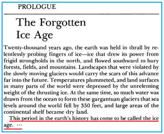
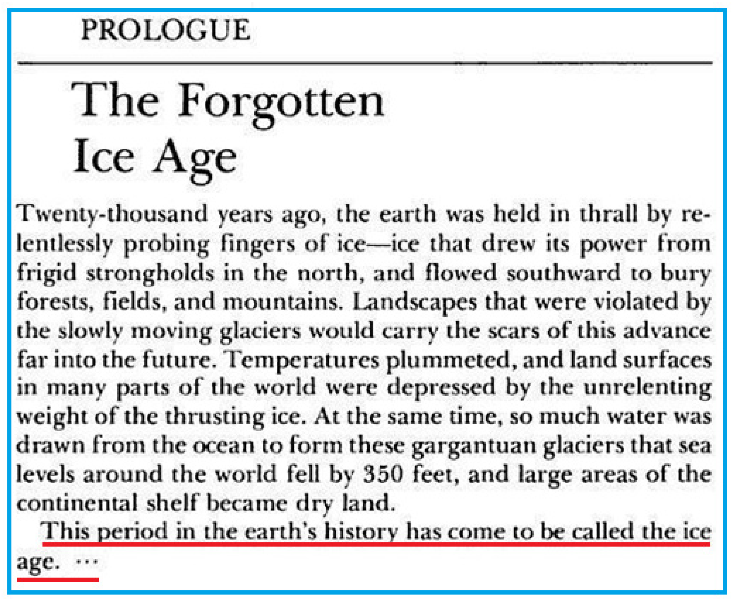
The Definition of the Ice Age used so far is too phenomenological, i.e., descriptive, as can be seen for example in Figure 11.
Figure 11.
The text above the red line is definition of the Ice Age that can be found in the Prolog of the famous book “Ice Ages—Solving the Mystery” by Imbrie and Imbrie [12].
After reading the text in Figure 11, it seems that it is time to position the new Definition of the Ice Age more as an astronomical–geophysical term and less as a phenomenological one [69]. For example, under the Ice Age are periods considered when there is “more” permanent ice, and there is permanent ice even when there is no Ice Age. Thus, this linguistic inconsistency should be replaced by some definition based on a full physical parameterization of the Ice Age phenomenon, which would achieve better alignment between measurement and theory.
8. Milanković, Serbia, Danube, and Loess
Much has been written about Milutin Milanković in a popular way, by himself [3] as well as others [7,70]. Also, Milanković is a well-known writer of popular scientific literature in the countries created by the former Yugoslavia [71].
It is known that Milanković loved Danube, which is quite understandable, because his life was connected to this river and cities on the Danube’s banks; he was bornin Dalj, studied in Vienna, was in Austro-Hungarian Empire captivity in Budapest during WWI where he wrote his first science book [8], and built his teaching and scientific career in Belgrade, Figure 7A. Figure 12 shows the steamship “Saturnus” on which he traveled, and about which he speaks in his correspondence with Wladimir Köppen and Alfred Wegener [5].
Figure 12.
The steamship “Saturnus” with which Milutun Milanković traveled along the Danube on the routes Belgrade, Dalj, Budapest, and Vienna in both directions, where from the ship he could see the impressive loess–paleosol profile of Stari Slankamen (Figure 13) on the right bank of the Danube at the mouth of the Tisza River, as well as other profiles that at that time hid evidence of the validity of his Ice Age Theory (Photo archive: N. Janc).
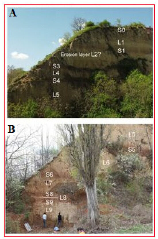
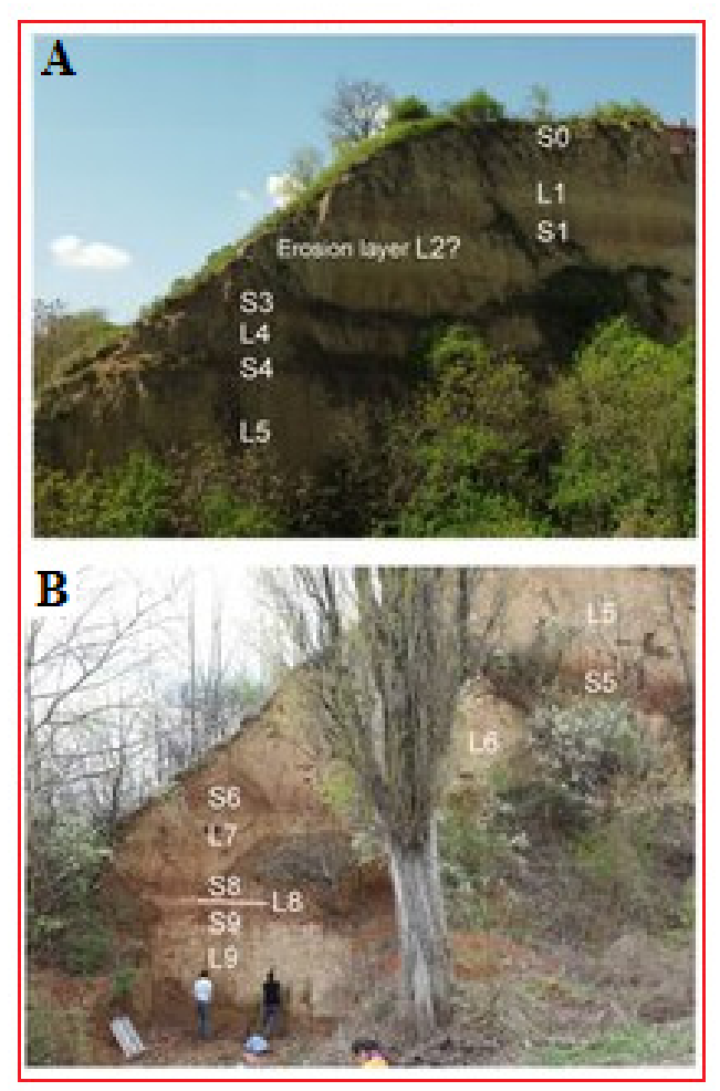
On those trips, Milanković had seen numerous loess–paleosol profiles on the banks of the Danube. He must have seen near the place of StariSlankamen an impressive loess hill dotted with horizontal stripes of light yellow and dark yellow color, placed as a natural artistic structure, something between a painting and a sculpture, perhaps as a kind of natural lighthouse, marking and decorating the confluence of the two mighty rivers Danube and Tisza, Figure 13. If he did not see the entire profile and all 9–10 layers of the loess–paleosol sequences, because the lower part of the profile has always been obscured by coastal vegetation and was difficult to see from the steamship “Saturnus”, he must have seen the upper part of the Stari Slankamen profile (Figure 13A) and several Ice Age (lighter—low values of Insolation and MS) and Inter Ice Age (darker—high values of Insolation and MS) periods.
Figure 13.
Two photos of the upper part (A) and the lower part (B) of Stari Slankamen loess profile on which the composite loess–paleosol sequences are clearly visible, where the lighter, yellow shades are loess layers, and the darker, brown shades are (paleo) soil layers, and all of the above is specially marked according to the nomenclature given in Figure 8, so that there are L1–L9, 9 loess layers (lighter) and S0–S9, 10 soil layers (darker) [44].
We cannot know Milanković’s impressions regarding this today. However, we do know that at the time, he was unaware that these layers represented paleoclimatic records. Perhaps, as a man with a deep connection to the Danube, he intuitively sensed that these loess–paleosol sequences were part of his Theory.
As is well known, Milanković [3] completely voluntarily and sincerely decided to investigate the climate of the distant past. It seems certain that he could not have known that in StariSlankamen there are confirmations of his “Ice” Theory, which place is located halfway along the Danube between Dalj, where he was born, and Belgrade, where he created his Theory. If Milanković’s Theory solved the “mystery of the Ice Ages”, it remains to solve the “mystery of Milanković and the Danube profiles”.
9. Conclusions
This research has three goals.
The first goalis to recall the circumstances of the creation of Milanković’s Mathematical–Astronomical Theory of Ice Ages with an emphasis on some unknown moments, such as the contributions of other scientists, as well as the important marking of the 50th anniversary of the verification of Milankovitch’s theory, also the important celebration of the scientist himself, rather like on James Croll (Wolfhill (Scotland), 1821—Perth (Scotland), 1890) in the Journal of Quaternary Science [72].
The second goal is to point out some evidence about the correctness of Milanković’s Theory on samples of Serbian loess. The visual similarity between graphs of Insolation and MS of Serbian loess indicates the correctness of Milanković’s Theory, and the comparison of the spectrum further confirms this. Malanković’s astronomicalforcing (eccentricity, obliquity, and precession) exists in the MS spectrum. In addition, MS reflects other forcings that Insolation does not have. This is to be expected, given that other forcings are not included in Milankovitch’s analyses. Such forcings are considered climate signals of unknown origin. This indicates the need for paleoclimate research, which, in addition to collecting new climate signals, should also aim for their causal interpretation.
The third goal is to point out the need to expand the basic postulates of Milanković’s Theory by combining as many astronomical and terrestrial processes and tuning them to the samples of climate signals. This could result in a more complete Theory, and the unknown climate signals might get a more certain causal interpretation.
Supplementary Materials
The following supporting information can be downloaded at: https://www.mdpi.com/article/10.3390/quat9060081/s1, S1: Interaction between Insolation and Loess Magnetization; S2: Hypothesis [59,73,74,75,76,77,78].
Funding
This research received no external funding.
Data Availability Statement
All used and listed (old) data can be found in the references listed here. The scientific results presented here, as an additional interpretation of old data, are found only in this paper.
Acknowledgments
I would like to thank the three anonymous reviewers for their useful comments and suggestions in the three rounds of manuscript review, as well as the Academic Editor who joined in the fourth and fifth rounds of review, which together made a great contribution to the final version of the manuscript, as well as Momčilo Gavrilov for his help in establishing the MS hypothesis.
Conflicts of Interest
The author declares no conflicts of interest.
Abbreviations
The following abbreviations are used in this manuscript:
| L | Loess |
| kyr | Units of one thousand years |
| MS | Magnetic susceptibility |
| N | North |
| S | Soil |
| USA | United State of America |
| V | Vojvodina |
References
- Milankovitch, M. Kanon der Erdbestrahlung und Seine Anwendung auf das Eiszeitenproblem; KöniglichSerbische Akademie: Belgrad, Serbia, 1941; 633p. (In German) [Google Scholar]
- Hays, J.D.; Imbrie, J.; Shackleton, N.J. Variations in the Earth’s Orbit: Pacemaker of the Ice Ages: For 500,000 years, major climatic changes have followed variations in obliquity and precession. Science 1976, 194, 1121–1132. [Google Scholar] [PubMed]
- Milanković, M. Memories, Adventures, and Gaining Insight from 1909 to 1944; Serbian Academy of Sciences: Belgrade, Serbia, 1952; 229p. (In Serbian) [Google Scholar]
- Köppen, W.; Wegener, A. Die Klimate der Geologischen Vorzeit; Verlag Von Gebrüder Borntraeger: Berlin, Germany, 1924; 256p. (In German) [Google Scholar]
- Janc, N.; Protić-Benišek, V.; Benishek, V.; Popović, L.Č.; Gavrilov, M.B.; Marković, S.B. Academicians Milutin Milanković and Vojislav Mišković: Correspondence about Alfred Wegener and Wladimir Köppen. Astron. Astroph. Trans. 2018, 30, 505–510. [Google Scholar]
- Janc, N.; Gavrilov, M.B.; Marković, S.B.; Protić-Benišek, V.; Benishek, V.; Popović, L.Č.; Tomić, N. Ice Age theory: A correspondence between Milutin Milanković and Vojislav Mišković. Open Geosci. 2019, 11, 263–272. [Google Scholar] [CrossRef] [Scilit]
- Janc, N.; Todorović, N.; Gavrilov, M.B.; Popović, L.Č. Milutin Milankovitch and Wenceslas Jardetzky—Scientific Collaboration; Lambert Academic Publishing: Saarbrücken, Germany, 2025; 123p. [Google Scholar]
- Milankovitch, M. Théorie Mathématique des Phénomènes Thermiques Produits par la Radiation Solaire; Académie Yougoslave Des Sciences et Des Arts, Gauthier-Villars et Cie: Paris, French, 1920; Volume XVI, 338p. (In French) [Google Scholar]
- eLibrary. 2026. Available online: http://elibrary.matf.bg.ac.rs/handle/123456789/702 (accessed on 25 July 2026).
- Imbrie, J.; Berger, A.; Boyle, E.A.; Clemens, S.C.; Duffy, A.; Howard, W.R.; Kukla, G.; Kutzbach, J.; Martinson, D.G.; McIntyre, A.; et al. On the structure and origin of major glaciation cycles 2. The 100,000-year cycle. Paleoceanogr. Paleoclimatology 1993, 8, 699–735. [Google Scholar] [CrossRef] [Scilit]
- Lisiecki, L.E.; Raymo, M.E. A Pliocene-Pleistocene stack of 57 globally distributed benthic δ18O records. Paleoceanogr. Paleoclimatology 2005, 20, PA1003. [Google Scholar] [CrossRef] [Scilit]
- Imbrie, J.; Imbrie, K.P. Ice Ages—Solving the Mystery; Macmillan: London, UK, 1979; 224p. [Google Scholar]
- Berger, A.; Loutre, M.F. Insolation values for the climate of the last 10 million years. Quat. Sci. Rev. 1991, 10, 297–317. [Google Scholar] [CrossRef] [Scilit]
- Laskar, J.; Robutel, P.; Joutel, F.; Gastineau, M.; Correia, A.C.M.; Levrard, B. A long-term numerical solution for the insolation quantities of the Earth. Astron. Astrophys. 2004, 428, 261–285. [Google Scholar] [CrossRef] [Scilit]
- Antoine, P.; Rousseau, D.-D.; Fuchs, M.; Hatte, C.; Gauthier, C.; Marković, S.B.; Jovanović, M.; Gaudenyi, T.; Moine, O.; Rossignol, J. High-resolution record of the last climatic cycle in the southern Carpathian Basin (Surduk, Vojvodina, Serbia). Quat. Int. 2009, 198, 19–36. [Google Scholar] [CrossRef] [Scilit]
- Basarin, B.; Vandenberghe, D.A.G.; Marković, S.B.; Catto, N.; Hambach, U.; Vasiliniuc, S.; Derese, C.; Rončević, S.; Vasiljević, D.A.; Rajić, L. The Belotinac section (Southern Serbia) at the southern limit of the European loess belt: Preliminary results. Quat. Int. 2011, 240, 128–138. [Google Scholar] [CrossRef] [Scilit]
- Bösken, J.; Klasen, N.; Zeeden, C.; Obreht, I.; Marković, B.S.; Hambach, U.; Lehmkuhl, F. New luminescence-based geochronology framing the last two glacial cycles at the southern limit of eouropeanpleistocene loess in Stalać (SERBIA). Geochronometria 2017, 44, 150–161. [Google Scholar] [CrossRef] [Scilit]
- Bronger, A. Zur quartären Klima- und Landschaftsentwicklung des Karpatenbeckens auf (paläo-)pedologischer und bodengeographischer Grundlage. In Kielergeographische Schriften; Selbstverlag Des Geographischen Instituts Der Universität Kiel: Kiel, Germany, 1976; Volume 45, 268p. [Google Scholar]
- Bronger, A. Correlation of loess-paleosol sequences in East and Central Asia with SE Central Europe—Towards a continental Quaternary pedostratigraphy and paleoclimatic history. Quat. Int. 2003, 106–107, 11–31. [Google Scholar] [CrossRef] [Scilit]
- Buggle, B.; Glaser, B.; Zöller, L.; Hambach, U.; Marković, S.B.; Glaser, I.; Gerasimenko, N. Geochemical characterization and origin of Southeastern and Eastern European loess (Serbia, Romania, Ukraine). Quat. Sci. Rev. 2008, 27, 1058–1075. [Google Scholar] [CrossRef] [Scilit]
- Buggle, B.; Hambach, U.; Glaser, B.; Gerasimenko, N.; Marković, S.; Glaser, I.; Zöller, L. Magnetic susceptibility stratigraphy and spatial and temporal paleoclimatic trends in East European loess paleosol sequences. Quat. Int. 2009, 196, 86–106. [Google Scholar]
- Buggle, B.; Glaser, B.; Hambach, U.; Gerasimenko, N.; Marković, S.B. An evaluation of geochemical weathering indices in loess-paleosol studies. Quat. Int. 2011, 240, 12–21. [Google Scholar] [CrossRef] [Scilit]
- Buggle, B.; Hambach, U.; Kehl, M.; Marković, S.B.; Zöller, L.; Glaser, B. The progressive evolution of a continental climate in SE-Central European lowlands during the Middle Pleistocene recorded in loess palaeosol sequences. Geology 2013, 41, 771–774. [Google Scholar] [CrossRef] [Scilit]
- Fitzsimmons, K.E.; Marković, S.B.; Hambach, U. Pleistocene environmental dynamics recorded in the loess of the middle and lower Danube basin. Quat. Sci. Rev. 2012, 41, 104–118. [Google Scholar] [CrossRef] [Scilit]
- Gaudenyi, T.; Nenadić, D.; Stejić, P.; Jovanović, M.; Bogićević, K. Stratigraphic revision of the Quaternary material from the vicinity of Belgrade and the Serbian segment of the Tisza valley analysed by V. D. Laskarev. Quat. Int. 2014, 357, 93–109. [Google Scholar] [CrossRef] [Scilit]
- Gaudenyi, T.; Nenadić, D.; Stejić, P.; Jovanović, M.; Bogićević, K. The stratigraphy of the Serbian Pleistocene Corbicula beds. Quat. Int. 2015, 357, 4–21. [Google Scholar] [CrossRef] [Scilit]
- Gavrilov, M.B.; Marković, S.B.; Schaetzl, R.J.; Tošić, I.A.; Zeeden, C.; Obreht, I.; Sipos, G.; Ruman, A.; Putnikovć, S.; Emunds, K.; et al. Prevailing surface winds in Northern Serbia in the recent and past time periods; modern- and past dust deposition. Aeolian Res. 2018, 31, 117–129. [Google Scholar] [CrossRef] [Scilit]
- Kostić, N.; Protić, N. Pedology and mineralogy of loess profiles et Kapela-Batajnica and Stalać Serbia. Catena 2000, 41, 217–227. [Google Scholar] [CrossRef] [Scilit]
- Marković, S.B.; Kostić, N.S.; Oches, E.A. Paleosols in the Ruma loess section (Vojvodina, Serbia). Rev. Mex. Cienc. Geol. 2004, 21, 79–87. [Google Scholar]
- Marković, S.; Oches, E.; Gaudenyi, T.; Jovanović, M.; Hambach, U.; Zoeller, L.; Sümegi, P. Paleoclimate record in the Late Pleistocene loess-paleosol sequence at Miseluk (Vojvodina, Srbija). Quaternaire 2004, 15, 361–368. [Google Scholar] [CrossRef] [Scilit]
- Marković, S.B.; McCoy, W.D.; Oches, E.A.; Savić, S.; Gaudenyi, T.; Jovanović, M.; Stevens, T.; Walther, R.; Ivanišević, P.; Galić, Z. Paleoclimate record in the Late Pleistocene loess-palaeosol sequence at Petrovaradin Brickyard (Vojvodina, Serbia). Geol. Carpath. 2005, 56, 483–491. [Google Scholar]
- Marković, S.B.; Oches, E.; Sümegi, P.; Jovanović, M.; Gaudenyi, T. An introductionto the Upper and Middle Pleistocene loess-palaeosol sequences of Ruma section (Vojvodina, Yugoslavia). Quat. Int. 2006, 149, 80–86. [Google Scholar]
- Marković, S.B.; Oches, E.A.; McCoy, W.D.; Gaudenyi, T.; Frechen, M. Malacological and sedimentological evidence for “warm” climate from the Irig loess sequence (Vojvodina, Serbia). Geophys. Geochem. Geosyst. 2007, 8, Q09008. [Google Scholar] [CrossRef] [Scilit]
- Marković, S.B.; Bokhorst, M.; Vandenberghe, J.; Oches, E.A.; Zöller, L.; McCoy, W.D.; Gaudenyi, T.; Jovanović, M.; Hambach, U.; Machalett, B. Late Pleistocene loess-paleosol sequences in the Vojvodina region, North Serbia. J. Quat. Sci. 2008, 23, 73–84. [Google Scholar] [CrossRef] [Scilit]
- Marković, S.B.; Hambach, U.; Catto, N.; Jovanović, M.; Buggle, B.; Machalett, B.; Zöller, L.; Glaser, B.; Frechen, M. The middle and late Pleistocene loess-paleosol sequences at Batajanica, Vojvodina, Serbia. Quat. Int. 2009, 198, 255–266. [Google Scholar] [CrossRef] [Scilit]
- Marković, S.B.; Hambach, U.; Stevens, T.; Jovanović, M.; O’Hara-Dhand, K.; Basarin, B.; Lu, H.; Smalley, I.; Buggle, B.; Zech, M.; et al. Loess in the Vojvodina region (Northern Serbia): An essential link between European and Asian Pleistocene environments. Neth. J. Geosci. 2012, 91, 173–188. [Google Scholar] [CrossRef] [Scilit]
- Marković, S.B.; Stevens, T.; Kukla, G.J.; Hambach, U.; Fitzsimmons, K.E.; Gibbard, P.; Buggle, B.; Zech, M.; Guo, Z.T.; Hao, Q.Z.; et al. The Danube loess stratigraphy—New steps towards the development of a pan-European loess stratigraphic model. Earth Sci. Rev. 2015, 148, 228–258. [Google Scholar]
- Marković, S.B.; Hao, Q.; Ludwig, P.; Zeeden, C.; Perić, Z.M.; Mihailović, D.; Radović, P.; Roksandic, M.; Lindal, J.; Krsmanović, P.; et al. 2026: Environmental dynamics recorded at Dupljaja loess section (southeastern Carpathian Basin, northern Serbia). Catena 2026, 263, 109732. [Google Scholar] [CrossRef] [Scilit]
- Marković-Marjanović, J. Contribution a l’Etude de la Constitution Geologique de Titelskibreg. Extrait du Bulletin de l’Academieserbe des sciences. Tome XII, nouvelle serie. Cl. Sci. Math. Nat. 1953, 3, 1–2. [Google Scholar]
- Nett, J.J.; Chu, W.; Fischer, P.; Hambach, U.F.; Klasen, N.; Zeeden, C.; Obreht, I.; Obrocki, L.; Pötter, S.; Gavrilov, M.B.; et al. The early Upper Paleolithic site Crvenka-At, Serbia–the first Aurignacian lowland occupation site in the southern Carpathian Basin. Front. Earth Sci. 2021, 9, 599986. [Google Scholar] [CrossRef] [Scilit]
- Obreht, I.; Zeeden, C.; Hambach, U.; Veres, D.; Marković, S.B.; Bösken, J.; Svirčev, Z.; Bačević, N.; Gavrilov, M.B.; Lehmkuhl, F. Tracing the influence of Mediterranean climate on Southeastern Europe during the past 350,000 years. Sci. Rep. 2016, 6, 36334. [Google Scholar] [CrossRef] [Scilit] [PubMed]
- Perić, Z.M.; Stevens, T.; Obreht, I.; Hambach, U.; Lehmkuhl, F.; Marković, S.B. Detailed luminescence dating of dust mass accumulation rates over the last two glacial-interglacial cycles from the Irig loess-palaeosol sequence, Carpathian Basin. Glob. Planet. Change 2022, 215, 103895. [Google Scholar] [CrossRef] [Scilit]
- Perić, Z.M.; Ryan, C.; Alexanderson, H.; Marković, S.B. Revised OSL chronology of the Kisiljevo loess-palaeosol sequence: New insight into the dust flux in the eastern Carpathian Basin during MIS 3-MIS1. Quat. Int. 2024, 698, 39–48. [Google Scholar] [CrossRef] [Scilit]
- Radaković, M.G.; Oches, E.A.; Hughes, P.D.; Marković, R.S.; Hao, Q.; Perić, Z.M.; Gavrilović, B.; Ludwig, P.; Lukić, T.; Gavrilov, M.B.; et al. Reconstructed Malacothermometer July Paleotemperatures from the Last Nine Glacials over the South-Eastern Carpathian Basin (Serbia). Atmosphere 2023, 14, 791. [Google Scholar] [CrossRef] [Scilit]
- Smalley, I.; Leach, J.A. The origin and distribution of the loess in the Danube basin associated regions of East-Central Europe—A review. Sed. Geol. 1978, 21, 1–26. [Google Scholar] [CrossRef] [Scilit]
- Smalley, I.J.; Marković, S.B.; Svirčev, Z. Loess is almost totally formed by the accumulation of dust. Quat. Int. 2011, 240, 4–11. [Google Scholar] [CrossRef] [Scilit]
- Stevens, T.; Marković, S.B.; Zech, M.; Sümegi, P. Dust deposition and climate in the Carpathian Basin over an independently dated last glacial-interglacial cycle. Quat. Sci. Rev. 2011, 30, 662–681. [Google Scholar] [CrossRef] [Scilit]
- Vandenberghe, J.; Markovič, S.B.; Jovanovič, M.; Hambach, U. Site-specific variability of loess and palaeosols (Ruma, Vojvodina, northern Serbia). Quat. Int. 2014, 334, 86–93. [Google Scholar] [CrossRef] [Scilit]
- Vidić, N.J.; Singer, M.J.; Verosub, K.L. Duration dependence of magnetic susceptibility enhancement in the Chinese loess-palaeosols of the past 620 ky. Palaeogeogr. Palaeoclimatol. Palaeoecol. 2004, 211, 271–288. [Google Scholar] [CrossRef] [Scilit]
- Vinnepand, M.; Laag, C.; Bosnić, M.G.; Ryzner, K.; Da Silva, A.-C.; Gavrilov, M.B.; Rolf, C.; Marković, S.B.; Ninkov, J.; Lagroix, F.; et al. Testing the sensitivity of geophysical proxies for climate reconstructions along a narrow precipitation gradient in the Middle Danube Basin. Quat. Res. 2026. first view. [Google Scholar] [CrossRef] [Scilit]
- Zeeden, C.; Hark, M.; Hambach, U.; Marković, S.B.; Zöller, L. Depressions on the Titel loess Plateau: Form–Pattern–Genesis. Geogr. Pannonica 2007, 11, 4–8. [Google Scholar] [CrossRef] [Scilit]
- Marković, S.B.; Jovanović, M.; Mijović, D.; Bokhorst, M.; Vandenberghe, J.; Oches, E.; Hambach, U.; Zöller, L.; Gaudenyi, T.; Kovačev, N.; et al. Titel loess plateau—Geopark. In Proceedings of the 2nd Conference on the Geo-Heritage of Serbia, Belgrade, Serbia, 22–23 June 2004; Institute for Nature Conservation of Serbia: Belgrade, Serbia, 2005; pp. 177–184. [Google Scholar]
- Marković, S.B.; Hambach, U.; Stevens, T.; Kukla, G.J.; Heller, F.; William, D.; McCoy, W.D.; Oches, E.A.; Buggle, B.; Zöller, L. The last million years recorded at the StariSlankamen loess-palaeosol sequence: Revised chronostratigraphy and long-term environmental trends. Quat. Sci. Rev. 2011, 30, 1142–1154. [Google Scholar] [CrossRef] [Scilit]
- Marković, S.B.; Hambach, U.; Stevens, T.; Basarin, B.; O’Hara-Dhand, K.; Gavrilov, M.M.; Gavrilov, M.B.; Smalley, I.; Teofanov, N. Relating the Astronomical Timescale to the Loess-Paleosol Sequences in Vojvodina, Northern Serbia. In Climate Change; Berger, A., Mesinger, F., Sijacki, D., Eds.; Part 2; Springer: Vienna, Austria, 2012; pp. 65–78. [Google Scholar]
- Tomić, N. Status and Perspectives of Geotourism Development in the Middle and Lower Danube Region in Serbia; Department of Geography, Tourism and Hotel Management, Faculty of Science, University of Novi Sad: Novi Sad, Serbia, 2021; 91p. (In Serbian) [Google Scholar]
- Heller, F.; Liu, T.S. Magnetostratigraphical dating of loess deposits in China. Nature 1982, 300, 431–433. [Google Scholar] [CrossRef] [Scilit]
- Kukla, G.; Heller, F.; Liu, X.M.; Xu, T.C.; Liu, T.S.; An, Z.S. Pleistocene climates in China dated by magnetic susceptibility. Geology 1988, 16, 811–814. [Google Scholar] [CrossRef] [Scilit]
- Maher, B.A. Magnetic properties of modern soils and Quaternary loessic paleosols: Paleoclimatic implications. Palaeogeogr. Palaeoclimatol. Palaeoecol. 1998, 137, 25–54. [Google Scholar] [CrossRef] [Scilit]
- Evans, M.E.; Heller, F. Environmental Magnetism: Principles and Applications of Enviromagnetics; Academic Press: San Diego, CA, USA, 2003; 299p. [Google Scholar]
- Gavrilov, M.B.; Marković, S.B.; Mladjan, D.; Zarić, M.; Pešić, A.; Janc, N.; Todorović, N. 2016: Global Warning–between the Myth and Reality. In Proceeding of International Scientific Conference “Archibald Reiss Days”, Belgrade, Serbia, 10–11 March 2016; Academy of Criminalistic and Police Studies: Belgrade-Zemun, Serbia, 2016; pp. 304–313. [Google Scholar]
- Lorenz, E.N. Deterministic nonperiodic flow. J. Atmos. Sci. 1963, 20, 130–141. [Google Scholar] [CrossRef] [Scilit]
- Gavrilov, M.B.; Jovanović, G.R.; Janjić, Z. Sensitivity of a long-range numerical weather forecast model to small changes of model parameters. Adv. Sci. Res. 2011, 6, 13–18. [Google Scholar] [CrossRef] [Scilit]
- Arakawa, A. Design of the UCLA General Circulation Model; Technical Report No. 7; Department of Meteorology, University of California: Los Angeles, CA, USA, 1972; 116p. [Google Scholar]
- Gavrilov, M.B.; Janjić, Z.I. Computed rotational energy spectra of two energy and enstrophy conserving schemes on semi-staggered grids. Meteorol. Atmos. Phys. 1989, 41, 1–4. [Google Scholar] [CrossRef] [Scilit]
- Lu, H.; Zhang, F.Q.; Liu, X.; Duce, A.R. Periodicities of palaeoclimatic variations recorded by loess-paleosol sequences in China. Quat. Sci. Rev. 2004, 23, 1891–1900. [Google Scholar] [CrossRef] [Scilit]
- Charney, J.G. Planetary fluid dynamics. In Dynamic Meteorology; Morel, P., Dordrecht-Holland, Eds.; D. Reidel Publishing Company: Dordrecht, The Netherlands, 1973; pp. 97–351. [Google Scholar]
- Rahmstorf, S. Ocean circulation and climate during the past 120,000 years. Nature 2002, 419, 207–214. [Google Scholar] [CrossRef] [Scilit] [PubMed]
- Gavrilov, M.M.; Basarin, B.; Hambach, U.; Machalett, B.; Gavrilov, M.B.; Marković, S.B. Paleoclimatic Record of the Titel Loess Plateau—From Depth to Time Scale. In Proceedings of the International Conference on Loess Research “Loessfest ‘09”, Novi Sad, Serbia, 31 August–3 September 2009; p. 82. [Google Scholar]
- Gavrilov, M.B.; Marković, S.B.; Gavrilov, M. Ice Ages—Definitions. In Proceedings of the Conference: 2nd Serbian Geographer’s Congress-Towards Europe, Novi Sad, Serbia, 10–11 December 2010; p. 52. [Google Scholar]
- Trifunović, D. From the correspondence of Milutin Milanković; BeoSing: Belgrade, Serbia, 2007; 320p. (In Serbian) [Google Scholar]
- Milanković, M. Through the Empire of Science—Pictures from the Lives of Great Scientists; Scientific Book: Belgrade, Serbia, 1950; 285p. (In Serbian) [Google Scholar]
- Edwards, K.J. ‘The most remarkable man’: James Croll, Quaternary scientist. J. Quat. Sci. 2022, 37, 400–419. [Google Scholar] [CrossRef] [Scilit]
- Boeglin, C.; Beaurepaire, E.; Halté, V.; López-Flores, V.; Stamm, C.; Pontius, N.; Dürr, H.A.; Bigot, J.-Y. Distinguishing the ultrafast dynamics of spin and orbital moments in solids. Nature 2010, 465, 458–461. [Google Scholar] [CrossRef] [Scilit] [PubMed]
- Tang, Y.; Jia, J.; Xie, X. Records of magnetic properties in Quaternary loess and its paleoclimatic significance: A brief review. Quat. Int. 2003, 108, 33–50. [Google Scholar] [CrossRef] [Scilit]
- Liu, Q.; Deng, C.; Torrent, J.; Zhu, R. Review of recent developments in mineral magnetism of the Chinese loess. Quat. Sci. Rev. 2007, 26, 368–385. [Google Scholar] [CrossRef] [Scilit]
- Maxbauer, D.P.; Feinberg, J.M.; Fox, D.L. Magnetic mineral assemblages in soils and paleosols as the basis for paleoprecipitation proxies: A review of magnetic methods and challenges. Earth-Sci. Rev. 2016, 155, 28–48. [Google Scholar] [CrossRef] [Scilit]
- Cullity, B.D.; Graham, C.D. 2008/2009: Introduction to Magnetic Materials, 2nd ed.; Wiley-IEEE Press: Hoboken, NJ, USA, 2009. [Google Scholar]
- Bradák, B.; Seto, Y.; Stevens, T.; Újvári, G.; Fehér, K.; Költringer, C. Magnetic susceptibility in the European Loess Belt: New and existing models of magnetic enhancement in loess. Palaeogeogr. Palaeoclimatol. Palaeoecol. 2021, 569, 110329. [Google Scholar] [CrossRef] [Scilit]


Disclaimer/Publisher’s Note: The statements, opinions and data contained in all publications are solely those of the individual author(s) and contributor(s) and not of MDPI and/or the editor(s). MDPI and/or the editor(s) disclaim responsibility for any injury to people or property resulting from any ideas, methods, instructions or products referred to in the content. |
© 2026 by the author. Licensee MDPI, Basel, Switzerland. This article is an open access article distributed under the terms and conditions of the Creative Commons Attribution (CC BY) license.