


Abstract
The paper presents a novel large language model-based neighbourhood search method for production scheduling using discrete-event simulation (DES) as the modelling and evaluation engine. The combination of large language models (LLMs) and DES represents a relatively new area of research with significant potential. The current study aims to demonstrate the applicability of LLMs for the automated closed-loop optimisation of production systems, using the DES environment as a configurable modelling tool and an evaluation engine at the same time, from which the results and the related contextual information are extracted at the end of each simulation run to provide feedback and context for the LLM in its autonomous search for improved solutions. The architecture was implemented with the use of Mistral Small 3.2 (24B) as the LLM and Siemens Tecnomatix Plant Simulation as the DES environment. The results from the proposed approach were compared with those of a genetic algorithm (GA) native to the applied DES environment, and with those achieved using simulated annealing (SA). While the proposed method was generally outperformed by the GA and the SA in terms of final solution quality and computational cost, it demonstrated advantages in terms of simulation demand while also providing a highly adaptable optimisation framework with significant potential for improvement and wider generalisation in the future.
1. Introduction
The application of large language models has become a major focus area in almost every scientific field in the recent period. One specific research domain where their utilisation is still relatively less explored is the area of discrete-event simulations. The defining attribute of these types of simulations is that they utilise a sequence of events for the modelling of a system, which also represents the changes in the model states. This makes the DES paradigm especially suitable for the modelling of large and complex systems with discrete operational states, such as production systems, material flow systems, telecommunication networks, patient-flows in healthcare, etc. The combination of DES and LLMs arose as a straightforward possibility from the previous, as LLMs excel in the identification and analysis of complex patterns such as those that characterise the operation of the above-mentioned systems.
The current paper presents a novel approach and a related framework for the combination of DES and LLMs with the aim of production scheduling optimisation, one of the typical application areas of the DES paradigm. A key characteristic of the proposed method is that the LLM executes a context-aware neighbourhood search on the space of possible production sequences, based on the information received from the discrete-event simulation model during each iteration step. Although this type of approach has rarely been tested, it provides unique insights into the capability of LLMs for understanding the underlying connections inherent in complex simulation models, demonstrating significant potential for future applications. In the current study, the proposed approach was tested on a typical compact production system layout implemented in Siemens Tecnomatix Plant Simulation, and the results of the optimisation runs were compared against those of an in-built genetic algorithm-based optimiser and also against those of a simulated annealing algorithm implemented in Python. These tests revealed valuable insights into the strengths and weaknesses of directly using LLMs for production schedule optimisation, while they also helped to identify multiple possible research directions. Altogether, the outcomes of the study provide multiple useful findings for guiding future research in this nascent but scientifically and practically important sub-field of LLM research.
The paper is comprised of seven sections. After the current introduction, in Section 2 the literature for the combined application of LLMs and DES is explored. Section 3 provides a general mathematical description of the production scheduling problem, while Section 4 presents the detailed description of the proposed approach and the related implementation framework. Section 5 presents the results of the optimisation runs with the proposed method, while Section 6 contains the discussion of the findings. Finally, the conclusions from the study are drawn in Section 7.
2. Combined Application of LLMs and DES in the Literature
Complex production planning, scheduling and plant-design problems have traditionally been addressed through a broad range of optimisation approaches, including both mathematical optimisation and simulation-based methods. Depending on the formulation of the optimisation problem, these approaches range from exact mathematical methods to metaheuristics and hybrid methods. While exact approaches guarantee optimal solutions, they often face computational limitations as problem complexity increases. In contrast, metaheuristics offer high-quality solutions with lower computational demands, though they do not guarantee a global optimum.
Various conventional optimisation approaches have been investigated in the context of complex production and process-engineering problems. Ponsich and Coello, for example, evaluated Differential Evolution for mixed-integer constrained process-engineering problems, comparing its performance with branch-and-bound and a genetic algorithm [1]. More directly in the context of simulation optimisation, de Carvalho Miranda et al. developed an adaptive genetic algorithm for the optimisation of discrete-event simulation models in manufacturing environments [2]. Hybrid approaches have also been investigated, including the matheuristic method proposed by Verbiest et al. for multiproduct batch-plant design [3]. In addition to algorithmic developments, computational acceleration represents another important research direction: Borisenko and Gorlatch compared GPU-parallelised metaheuristics with branch-and-bound for batch-plant optimisation [4] and subsequently investigated GPU-parallelised metaheuristics combined with parameter tuning [5]. These studies demonstrate the broad range of conventional optimisation strategies applicable to complex production and plant-optimisation problems, as well as the continuing importance of balancing solution quality, computational requirements and scalability.
Alongside these established optimisation approaches, the recent development of large language models has introduced new possibilities for supporting simulation modelling and optimisation through context-aware analysis and decision-making. Within this emerging research direction, several studies have investigated the combined application of LLMs and discrete-event simulation, particularly in material flow and manufacturing systems.
2.1. Examination of the Existing Literature on the Combined Application of LLMs and DES
Fei et al. presented an AI-assisted intelligent discrete-event simulation platform for manufacturing systems [6]. Their proposed architecture incorporates both simulation model generation and optimisation, although the latter relies on a single analytical step where the LLM evaluates the simulation results. In the provided case study, the authors utilised Claude model 3.5 Sonnet from Anthropic as the AI agent.
Reider and Lang presented a conceptual framework for automated simulation model generation (ASMG) in the field of production logistics, based on the application of generative AI [7]. Their framework is focused on the automated generation of simulation models based on knowledge bases, on user and on system prompts, though the iterative optimisation of the generated models would also be part of the functionality of the system. However, their study did not go beyond the conceptual phase in terms of implementation.
Li et al. presented a large manufacturing decision model (LMDM) architecture for human-centric decision-making [8]. Their approach combines LLMs with diffusion models to efficiently reconfigure manufacturing systems based on graphical and language inputs. Digital twin technology is applied for evaluating the decisions made by the LMDM and providing it with feedback (in the given example, a DES model implemented with Python was used to partially realise the functionality of the digital twin).
Jackson et al. applied the GPT-3 Codex for the automated generation of logistics simulations [9]. In their approach, the LLM produces executable Python code for the modelling of a given system, based on the input prompts and the provided model parameters. A number of simulation models created this way followed the discrete-event principle in their operation [9].
Frydenlund et al. also explored the possibility of using an LLM for simulation model generation as executable code [10]. In their research, they applied ChatGPT for this purpose. They asked the LLM to generate simulations in three modelling paradigms: discrete event, system dynamics and agent-based modelling. Their results showed that LLMs may not be fully effective in this form of simulation model generation at the time of the publishing of the paper, but they certainly have the potential for future improvements [10].
In their study, Romero-Guerrero et al. used ChatGPT for automated layout generation based on industrial drawings and documents [11]. Based on these inputs, the LLM generated code for FlexSim, a widely used discrete-event simulation environment. The results showed that this approach can aid in streamlining the simulation modelling process, especially when larger and more complex models are considered.
Elbasheer et al. also applied an LLM for the purpose of ASMG [12]. They presented a four-stage approach, in the implementation of which Siemens Tecnomatix Plant Simulation was used during model construction and execution. The authors applied Qwen 2.5 Coder in the role of the LLM. A main advantage of the proposed approach is that it facilitates ASMG based on the use of natural language, not requiring specific domain knowledge in simulation modelling.
Cirilli et al. presented a complex multi-agent-based scheduling framework for the automated generation of operational schedules from unstructured knowledge bases, mainly using LLMs for the implementation of the agents [13]. The scheduler agent also relies on a multi-objective heuristic search algorithm built with the NumPy and Pandas Python modules. A significant advantage of their method is that it can automatically generate schedules based on technical and operational manuals, which has clear industrial application potential. The authors demonstrated the application of their framework on a complex maritime case study.
Schmidt et al. presented a comprehensive generative AI-based framework for the automated generation, adaptation and evaluation of DES models in manufacturing [14]. The results proved that the method can successfully generate, adapt and evaluate simulation models, though not completely without errors, with the model generation phase being the most affected in this respect. Overall, the study proved that LLMs can be successfully applied for automated model generation, adaptation and evaluation with the support of a properly designed workflow and human-in-the-loop mechanisms.
Korth et al. presented a complex framework for supporting the simulation and exploration in production control and planning with LLM integration [15]. Their approach comprises four distinct modules aimed at supporting the simulation runs. Each of the supporting modules is integrated with the LLM, which in the conducted experiments was Meta Llama 3.1 70B. The results from the experiments demonstrated the applicability of LLMs as virtual assistants that can effectively support the simulation modelling process.
El Baz et al. presented an agentic optimisation framework integrating LLMs and DES for the solution of the storage location assignment problem in a forklift warehouse [16]. Their approach uses an LLM-based agent supported by human feedback for the creation of a Mixed-Integer Linear Programming model, which is then converted into executable Python code and solved with a commercial MILP solver. The results are evaluated with the application of a DES model. The conducted experiments demonstrated that the proposed method achieved clear improvements compared to the operational baseline.
Dehghani presented a framework named SimGPT, which integrates the Simio discrete-event simulation platform with LLMs (ChatGPT and Gemini) [17]. The most unique feature of the approach is that it allows the real-time integration of the LLMs with the simulation platform, which facilitates AI-supported decision-making during the actual runtime of the simulations. The proposed framework was tested on multiple case studies from different sectors, and these tests demonstrated the versatility of the approach from multiple aspects. One notable result was that in case of real-time job dispatching, the LLMs were able to outperform both three classical heuristics and two state-of-the-art metaheuristic optimisers.
Alshareef presented a framework for a bootstrapping, LLM-integrated iterative simulation generation and refinement method that also incorporates the use of the systems modelling language (SysML) and the discrete-event system specification (DEVS) formalism [18]. A main advantage of the proposed approach is that it enables the rapid development of executable simulation models from minimal textual input, with substantial automation of key steps [18]. The applicability of the method was demonstrated on a wafer fabrication example and on a large number of other examples from various domains as well.
Kute et al. also presented a framework for automated simulation model generation using LLM integration [19]. In their approach, the structured output of the LLM is evaluated and processed by a Python interpreter, which then instantiates the model in Siemens Tecnomatix Plant Simulation through the component object model (COM) interface. The optimisation of the model by the LLM is also a part of the functionality of the proposed framework, but at the time of writing of the paper the optimisation mechanism was in a conceptual phase and was manually guided by the user.
May et al. presented a framework for contingency management in production control based on the application of agentic LLMs [20]. In their approach, they used a localised LLM to collect past and current decision reasonings, sensory and simulation data in order to either derive a decision or a decision rule by the LLM itself (acting as an autonomous agent), or propose contingency management reactions for the human decision makers. For the validation of the proposed method, the Intel MiniFab was used as the underlying model simulated with Python.
Straka et al. examined the application of LLMs for autonomous model creation, output estimation from process descriptions and parameters, and copilot-guided manual building [21]. Specifically, they examined the application of Perplexity.ai and ChatGPT 5.2 in discrete-event simulation using ExtendSim 10 Pro 2024. Their results showed that while the LLMs could not autonomously design simulation models due to the lack of API (application programming interface) integration and produced a number of errors during output estimation, they can effectively accelerate model development for experienced users with the copilot-guided approach.
Premkumar et al. introduced three critical design principles for the integration of resilience and oversight into LLM-assisted Digital Twin development workflows [22]. These principles emerged from the iterative development and refinement of FactoryFlow, the authors open-source framework for building simulation-based Digital Twins of manufacturing systems using the DES paradigm with the integration of LLM-assisted structural modelling [22].
Thogaru et al. presented a closed-loop multi-agent framework named Warehouse AI for the planning and optimisation of warehouses, based on the combined use of DES, LLMs and knowledge-graph construction [23]. The agents in the framework are organised with the application of a LangChain hierarchy comprised of six specialised agents. The simulations themselves are realised using SimPy. The authors demonstrated the applicability of the framework using three different simulation scenarios and with clear positive results in all cases.
Wagenitz et al. proposed the combined application of LLMs and DES for risk detection and evaluation related to disruption risks for globally dispersed, project-driven supply chains [24]. Their approach is based on the automated generation of simulation blueprints by the LLM, based on the disruption signals received by the latter. The generated simulations represent two scenarios, a baseline and a disruption scenario. The simulation generation is realised using SimPy, while the risk evaluation itself is based on Monte Carlo experimentation. The authors demonstrated the applicability of the approach through a case study on Red Sea piracy disruptions.
While the previously discussed literature has concentrated on the application area of material flow systems (mostly manufacturing and production systems), it is important to highlight that the combined use of DES and LLMs extends to a much wider variety of applications, as illustrated by the following studies.
Jadhav et al. examined the potential of using LLMs for High-Performance Computing (HPC) job scheduling [25]. In their approach, the HPC environment was modelled with a discrete-event simulation, while LLMs were applied to make job scheduling decisions. The results derived from multiple simulated scenarios showed that on the one hand, LLMs can be effective at making job scheduling decisions in complex HPC environments, but on the other hand, current cloud-based LLM services impose significant latency constraints limiting real-time deployment, though there is a clear potential for further improvement.
Miski et al. applied an LLM-based automated simulation generation approach for the modelling of healthcare systems [26]. They modelled two types of systems, a skin care clinic and a complex medical care facility. The LLM was applied to produce simulations in the form of Python codes based on the user prompts. The results of these simulations were compared with those from Arena, a widely utilised discrete-event simulation software. The overall results of the comparison showed that the LLM was able to achieve similar results produced by the DES environment, while it also successfully determined the optimal resource allocation to minimise costs and at the same satisfy the patient waiting time constraints.
Diamatopoulos et al. presented a conceptual framework for the LLM-augmented discrete-event simulation of blockchain systems [27]. In their concept, the application of LLMs together with DES for blockchain modelling can have two main use cases: dynamic simulation scenario generation and malicious node modelling and cooperation attacks. In the proposed conceptual architecture, the blockchain simulator SymBChainSim would interface with two LLMs which would implement the previously described functionalities.
Katale et al. presented a hybrid simulation framework integrating DES, microscopic pedestrian simulation and LLMs for the analysis of the propagation of cyber disruptions through passenger-facing airport operations [28]. The DES layer in the framework models the service processes, while the pedestrian layer models the passenger movements. The role of the LLM is to generate post-security decisions in relation to the passengers. The framework was evaluated through a case study with one baseline and multiple disruption cases. The results of this case study and additional validations demonstrated the ability of the framework to produce plausible disruption patterns [28].
Monks et al. applied LLM-based automated simulation generation for a unique purpose, to recreate published discrete-event simulation models using Free and Open-Source Software (FOSS) based on the descriptions available in academic journals [29]. They specifically focused on models found in Healthcare Operations research. They proposed a four-stage approach for model recreation and successfully recreated two simulation models (a critical care unit and a stroke pathway capacity planning model) using Perplexity as the LLM, and Python 3.10 and SimPy 4 codes as output formats.
Mattar et al. proposed a fog-based architecture integrated with an LLM to safeguard the confidentiality, integrity, and availability of outsourced cloud data [30]. As part of the operational pipeline of the framework, the LLM executes a multi-phase reasoning process that includes load analysis, security scrutiny, Quality of Service (QoS) prioritisation and scheduling recommendations, based on the previously gathered context vectors. The LLM continuously refines its decision boundaries based on user-defined policies and observed network performance. The framework is evaluated with a custom edge-cloud discrete-event simulator built on Python 3.9 [30].
In their paper, Liu et al. explored how the integration of agent-based modelling (ABM) with LLM-driven autonomous agents can have a transformative effect on social simulation, especially in the context of the United Nations sustainable development goals (SDGs) [31]. They proposed a framework for the integration of LLMs into ABM, the core engine of which manages a discrete-event simulation environment. They provided a detailed description of the proposed framework and explored its application possibilities in policy co-creation, inclusion, and automation.
Neto et al. presented an LLM-based tool called GEM DEVS Chat for the specific purpose of assisting developers in understanding DEVS models within a simulation project [32]. The tool was designed to aid in the understandability of models written in DEVS Natural Language (DNL) and deployed on the MS4 Me platform. They demonstrated the applicability of the approach through a controlled experiment involving eight students. The results proved that the students who used the framework were indeed able to understand DEVS models more quickly and accurately.
Vicente-Martínez et al. proposed a Conversational Digital Twin Framework (CDTF) that integrates generative AI with simulation-based decision support for the aid of operational planning of large-scale events [33]. Their framework consists of four layers: a data integration layer, a simulation engine combining machine learning and DES components, a conversational AI interface and a visualisation layer for reports and dashboards. In the concrete implementation, the simulation engine was realised with the application of Random Forest models and DES components. The proposed framework was evaluated through a case study focused on the Gran Canaria Stadium.
Besides of the previously discussed literature, it is also important to note that another significant application area of DES is the modelling and optimisation of LLM inference serving, which can be found in multiple studies, for example in the papers of Patel et al. [34], More et al. [35] and Jaiswal et al. [36], among others. While this is an especially important field of application connected to LLMs in general, it does not directly relate to the topic of the current study, which is focused on the direct combination of LLMs and DES for solving optimisation problems.
2.2. Contributions of the Current Study
As can be seen from the analysed literature, a significant number of studies focused on automated simulation model generation with the aid of LLMs. While these frameworks often contain optimisation features as well, these are usually realised in the form of recommendations made by the LLM for the human evaluators, often based on a single analytical phase of the simulation model. A number of studies applied discrete-event simulation as a modelling tool used in the evaluation of the performance of LLMs in sector-specific applications, for example in case of [28,30]. Some studies also employed LLMs as interactive agents in the simulation model, for example in the case of [17,26]. While the latter represents a form of automated optimisation of model parameters by the LLMs, the closed-loop autonomous LLM-based optimisation of fixed model attributes through an iterative improvement process using consecutive simulation runs remains largely unexplored. One exception to this is the work of Thogaru et al. [23], in which the proposed architecture is capable for the autonomous iterative improvement of the simulation model based on the evaluation results of the previous cycle, but it is based on the use of multiple agents, knowledge graphs, graph reasoning and a LangChain, and is also focused more on warehouse planning. In contrast, the current work can be viewed more as a metaheuristic guided by a single LLM-agent. Recently, LLM-guided neighbourhood search approaches were proposed by others as well, for example in [37], but these methods optimise scheduling problems directly rather than through a discrete-event simulation model and for this reason do not incorporate simulation-derived operational feedback. Therefore, the contributions of the current study can be summarised as follows:
- Demonstration and proof-of-concept of the LLM-based closed-loop autonomous optimisation of fixed model attributes through iterative improvement using consecutive simulation runs, based on the application of a single LLM-agent and structured textual information. In the present study, the optimised attribute is the pre-planned production schedule of the manufactured parts in the model. The proposed optimisation algorithm can effectively be described as a context-aware LLM-guided neighbourhood search heuristic.
- Detailed description of the presented LLM-guided scheduling framework, including the architecture and the principal technical solutions employed in its proof-of-concept implementation.
- Identification of the observed advantages of using LLMs in the aforementioned way for the optimisation of discrete-event simulation models, based on the comparison with two standard heuristic approaches (genetic algorithm and simulated annealing) serving as benchmark methods. The comparison itself is realised through a series of optimisation runs executed using all three methods.
- Identification of future research directions and exploration of the application potential of the proposed LLM-based optimisation approach, including its applicability to a wider scope of problems.
3. Description of the Production Scheduling Problem Examined in the Current Study
The production scheduling problem is one of the classic problems of operations research, one which is also fundamentally important for the manufacturing sector. While it can have many variations, in the followings the standard mathematical description of the problem will be given. Let:
be the set of jobs (parts) and
be the set of machines (stations).
Each job consists of an ordered sequence of operations:
and denotes the processing time of operation of job .
The decision variable is the production sequence:
where represents the job released in position .
The primary objective is minimising the makespan:
where is the completion time of job as a function of .
The optimisation objective is therefore:
where is the set of feasible production sequences.
Usually, each job represents a concrete manufacturing process, as is the case in the current study. Therefore, operations of a job must follow their prescribed route, which can be formulated as the following constraint:
where is the start of operation and is the completion time of operation i.
In the current study, the transportation of the parts is modelled with the application of workers for added realism. In addition, each manufacturing station can only work on one part at a time. It is also important to note that there is a total of 64 parts in the production schedule, which all have to be finished at the end of a simulation run. Therefore, the objective function (6) in the current study is also subject to the following constraints besides (7):
- machine-capacity constraints,
- worker-availability constraints,
- completion of all 64 parts.
While the total number of parts is 64, these are comprised of eight types of parts, and there are eight pieces from each type. Therefore, the production sequence in the current problem is a permutation of a multiset. Because of this, the total number of possible production sequences can be calculated as:
It is evident that this is an astronomical number which makes a brute-force exact simulation-based approach (or any other brute-force exact modelling approach) impossible. At the same time, production scheduling problems like this represent a crucially important problem-set for virtually every manufacturing company. These are exactly the reasons why heuristics and metaheuristics—such as the method proposed in the current paper—are often necessary for solving this type of problem, and why production scheduling is one of the key application areas of DES based modelling supported by optimisation algorithms.
4. Presentation of the Concept and the Components of the Proposed LLM-Guided Neighbourhood Search Method and the Related Framework
4.1. Introduction of the General LLM-Guided Scheduling Framework
The proposed LLM-guided neighbourhood search method is realised through the implementation and utilisation of a multi-component framework presented below in Figure 1.
Figure 1.
The architecture of the complete LLM-guided scheduling framework with its main components. The optimiser generates the original log files in CSV format, while ‘xml’ in the output box refers to the Office Open XML (.xlsx) spreadsheet versions used for subsequent data processing and analysis.
As can be seen, the central component of the framework is the LLM-guided optimiser, which connects a local LLM with the DES model of the examined production system. The use of a local LLM was mainly chosen on the grounds of better reproducibility, while it also makes the performance comparison between the proposed method and the two standard heuristics (GA and SA) more straightforward. For the proof-of-concept implementation of the framework, Mistral Small 3.2 (24B) (24 billion parameters) was chosen as the given LLM, as it strikes a good balance between performance, robustness and resource-efficient local deployment. Ollama was used as the local LLM inference framework to run the model; multiple Ollama versions were used during the experimental period, and compatibility was subsequently verified with version 0.34.0.
The main role of the LLM-guided optimiser is to extract the results—the makespan and the utilisation data of the manufacturing stations—at the end of each simulation run from the DES model, transfer this data to the LLM in the form of a structured prompt about the optimisation task expanded with a utilisation summary, a bottleneck summary and the results from previous iterations (these will be described in detail in Section 4.3), then send back the new production schedule proposed by the LLM to the DES model and run the simulation again with the new sequence. If the LLM cannot improve the makespan after a certain number of iterations, the process is restarted with the initial production sequence (this way, the proposed method utilises a multi-start approach). This iteration loop continues until the number of iterations reaches a predefined limit which can be set (together with other parameters) in the code of the optimiser. The optimiser itself is implemented in Python (version 3.13.14). The communication between the different software components is realised with the application of the component object model (COM) interface. At the end of a complete optimisation run, the final global best makespan is written out by the optimiser, together with the logs data and the raw LLM replies.
The operation and the characteristics of the LLM-guided optimiser will be described in detail in Section 4.3, together with the exact neighbourhood search algorithm it implements. Before that, in the upcoming Section 4.2 the production system DES model created for the proof-of-concept implementation of the framework is going to be presented.
4.2. Presentation of the Simulation Model Used in the Implementation of the Framework
The DES model created for the proof-of-concept implementation of the framework represents a standard flexible manufacturing layout with twenty manufacturing stations, one source (from which the raw materials originate) and one drain (where the finished products leave). The model was created with the Siemens Tecnomatix Plant Simulation software (version 2404). The layout of the model from a top-down view can be seen in Figure 2.
Figure 2.
The top-down view of the production system DES model created for the proof-of-concept implementation of the framework.
The material flow between the stations is realised with the aid of workers, who carry the parts in-between the stations (and also from the source, and to the drain). Each worker can carry only one part at a time, and each station can only work on a single part at a given time as well. As it was mentioned in Section 3, there are eight types of parts and there are eight units from each part type, which equals to a total of 64 elements in the production sequence. In Figure 3 below, the visualised operation of the model can be seen during a simulation run (it is important to note that during the optimisation run with the LLM-guided scheduling framework, the simulations are not visualised, instead they are repeatedly performed in memory after their initialisation).
Figure 3.
Three-dimensional view of the production system DES model during a visualised simulation run.
In the followings, a non-exhaustive list of the main objects in the simulation model will be presented together with their short descriptions:
- Source: The object from which the parts originate. In the given model, the source is set to generate a new part precisely in every three minutes, regardless of the part type.
- Stations: The stations represent the manufacturing stations in the model. In the given setting, they represent completely automated workstations, which only require human operators for the loading and unloading of parts. Each station can only work on a single part at a given time. There are a total of twenty stations in the model.
- Drain: The exit point for the finished parts where they “leave” the model. Each part is eventually transported to the drain. It is accessed through a Buffer object connected to it. The use of the Buffer is not mandatory; it was only used in the current model to follow standard practice. Its application could be useful for example to prevent upstream blocking and manage the drains capacity under certain drain-settings, even though the exploration and analysis of such situations was not part of the current study as the drain processing time was set to 0.
- WorkerPool: The object from which the workers enter into the model. It can generate an arbitrary number of workers, but based on the experience from the initial simulation runs, at least three workers are required in the current model to avoid any deadlock situations. Under the settings used in the current study, the workers always start from the worker pool and once they finished their assignment, they also return to it (unless a new task for them emerges in the meantime). As the workstations in the current model are conceptualised to be automated, the workers do not have to wait at the stations for the completion of a manufacturing job; instead, they return to the worker pool once they finished their transportation tasks.
- SourceSequence: One of the most important elements of the model, as this data table contains the production sequence for the Source object, which is also the target of optimisation. While each part type in the sequence also has a separate object class created for it, the actual prescribed routes for the parts are related to the third column of the table, which contains the names of the part types in a string format.
- Processes: This data table contains the actual routing data for the part types through nested tables. It is connected to the third column of the SourceSequence table indirectly through a control method of the Broker object, which selects the next destination for a part on completion of a job based on the part’s name (which is given during the parts creation at the Source according to the SourceSequence table) and the connected nested routing table in the Processes table.
- Broker: The Broker object is responsible for the task management of workers in accordance with the task requests by the resource objects (in the current simulation, these are the Source, the Stations and the Drain). Through a custom control method, in the current simulation it is also responsible for the routing of the parts based on the Processes table.
- EventController: The EventController is a fundamental part of every Plant Simulation model, as it effectively drives the discrete-event simulation process and measures the elapsed time. In the proposed LLM-guided optimisation framework, it is also used for the extraction of the makespan data from a completed simulation run, as the latter is effectively the same as the elapsed time during the simulation run, which is measured by the EventController.
- Chart: The chart object is used to produce the utilisation data of the resource objects in a model, which in this case the utilisation data of the manufacturing stations. As the name of the object implies, it can represent this data in the form of a bar chart, but the main use of the object in the current model is to write this data into the ResourceStatistics table through a custom EndSim method.
- ResourceStatistics: The ResourceStatistics table contains the utilisation data of the Stations in a numerical format. It is written into the table and extracted by the LLM-guided optimiser at the end of each simulation run. The optimiser then provides a summary of the utilisation statistics to the LLM based on the extracted data.
- FlatProcessTable: This table contains effectively the same data as the Processes table, but in a single layer without the use of nested tables. It is used by the LLM-guided optimiser at the beginning of the optimisation run to extract the routing data from the model for each part, and share it with the LLM. For the purpose of reproducibility, the complete contents of the FlatProcessTable are also included in Appendix C (Table A1) to provide a full picture of the manufacturing process steps of each part type.
- ExitedParts: This variable is used for counting the finished parts exited at the drain. Its main use is to validate the successful completion of the production schedule (when the value of the variable reaches 64), which is important for the validation of the given production sequence provided by the LLM. If the simulation ends before the variable reaches 64, that means that either a deadlock occurred which prevents the completion of the schedule, or the proposed sequence did not contain 64 elements (though the latter is also checked by the optimiser separately) and for these reasons the sequence cannot be accepted as a valid solution regardless of the makespan value.
- GAWizard: The GAWizard object implements the native genetic algorithm that can be used in Plant Simulation to optimise the selected parameters of a given model. The tool among other settings allows the definition of the optimisation parameters, the selection of the number of generations, the size of each generation and the weighting of the fitness calculation if there are multiple optimisation parameters. In the current model, the single optimisation parameter is the simulation time, which is the same as the makespan (the simulation starts with the generation of the first part at the Source and ends with the exit of the last finished part at the Drain). The main role of the GA in the current study is to provide a comparison benchmark for the proposed LLM-guided optimisation algorithm.
- CompletedSims: This variable is used for counting the completed simulation runs during an optimisation run with the GAWizard (it is incremented every time by one when a simulation run is finished). This data is important for the comparison of the proposed LLM-based method with the GA. It must be noted that as the variable only counts the completed number of simulations till a predefined threshold configured in the EndSim method is reached, therefore the required simulation numbers for reaching the designated thresholds during the optimisation experiments were incremented by one in case of the GA before being presented in Section 5, in order to include the actual simulations that first reached the given thresholds as well (the simulation counts related to the proposed LLM-based method are recorded directly by the LLM-guided optimiser using a different logging mechanism). For the threshold corresponding to the best GA solution, the displayed makespan value reported by the GAWizard (version 2404)was rounded. Therefore, where necessary, the threshold used during post-processing was increased by one unit in the last reported decimal place to ensure that the corresponding simulation run was correctly identified.
4.3. Detailed Description of the LLM-Guided Optimiser
As it could be seen in the earlier description of the overall LLM-guided scheduling framework, the core element of the architecture is the optimiser, which not only connects the LLM with the DES model, but also extracts the necessary data from the simulation model during each iteration and processes it in order to provide structured written information for the LLM about the performance of the production system.
The code for the optimiser was written in Python. During the implementation of the proposed optimiser, ChatGPT (OpenAI; GPT-5 series) was used solely as a software development support tool for code implementation, debugging, and technical discussion. As described in Section 4.1, the complete LLM-guided scheduling framework itself which is introduced and evaluated in this study employed Mistral Small 3.2 (24B) during runtime.
In the upcoming Section 4.3.1, the algorithm of the optimiser will be described in detail. Utilising the embedded prompt provided for the LLM, the optimiser effectively implements the proposed LLM-guided neighbourhood search algorithm. The structure of the prompt itself will be described in Section 4.3.2, while the complete text of the prompt can be found in Appendix A.
4.3.1. The Algorithm of the LLM-Guided Optimiser
The complete high-level algorithm realised by the LLM-guided optimiser is presented in Figure 4, which is preceded by the description of each step of the presented algorithm:
Figure 4.
The high-level algorithm of the LLM-guided optimiser.
- Start: The start of the algorithm, which in the current implementation effectively means running the Python code of the optimiser.
- Log file initialisation: The algorithm initialises the log files, a CSV file for logging the data related to each iteration of the optimisation run and a JSON file for logging the replies of the LLM. The CSV file has a significant number of columns, which among others contain the proposed action by the LLM regarding the production sequence (the possible types of actions will be described later at step 6. and also in Section 4.3.2), the iteration number (both the global iteration number and the one in the current restart), the search mode (normal or diversification mode), the makespan for each candidate proposed by the LLM in an iteration, the best makespan in the current iteration and the global best makespan, the elapsed time in the optimisation run (together with the simulation time and the LLM reply time in each iteration), in addition to a large number of additional information related mainly to the validation of the answers and the simulation runs.
- Connecting to the Plant Simulation model, setting the initial production sequence: The optimiser connects to the Plant Simulation software through the COM interface, opens the model and sets the production sequence to the initial repeating alpha-numerical order (the eight types of parts in alpha-numerical order, which itself is repeated by eight times, resulting in a 64-element production sequence).
- Initial simulation run, extracting the makespan and the utilisation data: The optimiser runs the simulation with the initial production sequence, then extracts the makespan and the utilisation data of the workstations from the model.
- Start of the optimisation run in normal mode: After the results from the initial simulation run are received, the optimiser starts the optimisation run in normal mode. There are essentially two search modes in the proposed neighbourhood search method, normal and diversification mode, which mainly differ from each other in the number of proposed candidate solutions by the LLM and in the transformative effect of the proposed actions (these will be described later in more detail in step 22).
- Providing the LLM with the description of the optimisation task and the makespan of the last best candidate: In many ways, this step is the most central part of the proposed algorithm, as the LLM receives the embedded prompt from the optimiser in this phase. Technically, steps 7 and 8 represent sections of the prompt as well, but for the purpose of better readability, they are described as individual process steps following 6. Describing the entire prompt here would simply be unfeasible; therefore, the prompt structure is presented in detail separately in Section 4.3.2, while the entire text of the prompt can be found in Appendix A. From an algorithmic perspective, the most important aspect of the prompt is that it contains the description of the optimisation task the LLM has to solve, while it also contains the extracted and processed information from the previous best candidate solution as well (this can also be the initial simulation run if the optimisation process has just started or restarted). The most important part of the task description is the definition of the possible actions the LLM can implement on the production sequence of the last best solution (which itself was either proposed by the LLM in a previous iteration step of the optimisation run, or it is the initial sequence in case the optimisation run has just started or restarted). Basically, the LLM can implement five types of actions on the sequence, through which the neighbourhood search strategy is implemented based on the context provided by the information from the last best solution (and from the last two best solutions in the form of the trend summary). These actions are the following:
- move: move one element of the sequence to a new position
- swap: swap two elements of the sequence
- reinsert (move) block: reinsert a block of elements elsewhere into the sequence
- reverse: reverse the elements in a block
- swap blocks: swap two blocks of elements in the sequence
Out of these, the first two are preferred in normal mode, while the use of the other three is encouraged more in diversification mode.
The context based on which the LLM chooses from the previous actions is provided by the utilisation and bottleneck summaries of the last best candidate, and by the trend summary related to the changes between the last two best solutions. In essence, the utilisation summary provides a global context for the LLM, while the bottleneck summary gives a more focused context containing the most utilised stations and the part types associated with each bottleneck station. In addition, historical data regarding the recent moves proposed by the LLM are also included in the prompt (these will be described in detail in Section 4.3.2).
- 7.
- Providing the LLM with the utilisation summary and the bottleneck summary of the last best candidate: As it was mentioned, technically the utilisation and bottleneck summaries also form parts of the previous step together with the trend summary, but from a readability perspective it was better to move these into separate process steps in the algorithmic chart. The utilisation summary contains the textual description of the states of the top three “working”, “waiting” and “blocked” stations, giving the ratios in percentages (“waiting” means the station waits for the next task or part, while “blocked” means that it is waiting for unloading in order to be able to receive the next part). The bottleneck summary contains the textual description of the most heavily utilised stations from the combined aspects of the “working”, “waiting” and “blocked” states, and the processed parts together with the related manufacturing process information (the manufacturing time and the process step identifier) in case of each station. The bottleneck summary can contain a maximum of ten stations (in the standard settings, it actually combines the top five stations from each mentioned aspect, but this results in a total maximum of ten stations appearing in the summary). It must be noted that the numbers of stations appearing in the summaries are modifiable parameters, but the numbers given above were used as standard settings during the experiments.
- 8.
- Providing the LLM with a trend summary based on the previous and the current results: The trend summary describes the changes occurred between the last two best candidates which produced an improvement in the makespan in a textual format. The summary lists the top five stations both in terms of the change in the “blocking”, “waiting” and “working” percentages. It is worth mentioning that during runtime, whenever an improvement occurs in an iteration of the optimisation run, the utilisation, bottleneck and trend summaries are all written out in the terminal of the integrated development environment (IDE) as well.
- 9.
- Validation of the answer from the LLM: Based on the information received in steps 6, 7 and 8 (as was mentioned, technically all of this information is provided in a single prompt), the LLM proposes a new action from the list of possible actions. However, the answer of the LLM must be validated before the further progression of the algorithm. The validation effectively takes place on three successive levels:
- First, the response validity is checked based on the anticipated JSON syntax and the required fields.
- Secondly, the proposed action is validated in terms of whether it satisfies the allowed move definitions and parameter constraints (for example, all indices used in the actions regarding the proposed sequence change must be in the 0 to 63 range).
- Thirdly, the schedule validity is checked. This means that the generated production sequence must contain all required parts exactly once per occurrence and it must have the correct length (64). It also must be a novel sequence, one that has not been evaluated previously (repeated actions with the same parameters applied on the same production sequence are flagged as duplicates).
- 10.
- Is the answer valid: If the answer was determined to be valid the algorithm continues with step 11, otherwise with step 27.
- 11.
- Extracting one candidate production schedule from the answer: In case the answer of the LLM was valid, the optimiser builds the new production schedule from the answer’s content. It is important to highlight that the LLM only provides a proposed action in its answer and it is the optimiser’s task to create the new sequence based on that action and the previous production sequence.
- 12.
- Expanding the logs and the raw LLM replies file: The optimiser expands the contents of the CSV log file and the JSON file (the latter containing the LLM’s answers) with a new entry related to the newly proposed candidate sequence. In addition, it is important to note that a separate summary record is also appended after the completion of a full iteration (depending on the search mode, a full iteration contains either five or ten proposed candidate sequences under the settings used in the conducted optimisation runs).
- 13.
- Was the stagnation threshold reached?: During the optimisation run, if there was no improvement in the makespan after the completion of a certain number of iterations (each containing multiple proposed candidates), the algorithm switches from normal to diversification search mode. Step 13 checks whether this threshold was reached (in the conducted experiments, this threshold was set to 3).
- 14.
- Was the restart stagnation threshold reached?: The algorithm implements a multi-start approach in order to avoid the situation of being stuck in a local minimum. In order to achieve this, after a certain number of iterations without improvement in the makespan the optimisation process restarts entirely from the initial production sequence. Step 14 checks whether this threshold was reached (in the conducted experiments, this threshold was set to 10).
- 15.
- Running the simulation for the validated candidate and extracting its makespan and utilisation data: The optimiser runs the Plant Simulation model with the newly proposed candidate sequence and extracts the makespan and the utilisation data of the stations at the end of the simulation run. It is important to note that at the end of each simulation run, the number of manufactured (exited) parts is also checked to avoid such cases where a deadlock situation might prevent the completion of the entire proposed production schedule, yet the proposed candidate is still accepted as a valid solution.
- 16.
- Was the candidate limit reached?: In this step, the algorithm checks whether the candidate limit was reached in the current iteration, depending on the search mode. If this limit was reached, the algorithm continues with step 17.
- 17.
- Selecting the best candidate in the iteration, updating the best makespan in the current iteration run and the global best makespan: The best candidate (the one with the shortest makespan) is selected from the candidates proposed during the current iteration. If this candidate is better than all other results in the current iteration run since the last restart (or since the start of the entire optimisation run if there was no restart so far), then the best makespan for this iteration run is updated. If this makespan is also the best since the start of the entire optimisation run counting all restarts, then the global best makespan is also updated with this result.
- 18.
- Increase the global iteration number by one: After the completion of the current iteration of the optimisation process, the number of finished iterations during the optimisation run is increased by one (both globally and in the current iteration run since the last restart).
- 19.
- Was the global iteration limit reached?: The algorithm checks whether the limit of the number of iterations in the optimisation process was reached (during the conducted experiments, this limit was set as 100).
- 20.
- Did the best makespan improve in the recently finished iteration?: The algorithm checks whether the best makespan was improved in the recent iteration compared to the previous best makespan (the best makespan in the iteration run since the last restart). While the best makespan was already updated in step 17, the check in the algorithmic chart here serves the purpose of determining whether the no improvement counter should be increased.
- 21.
- Increase the no improvement counter by one: If the best makespan did not improve in the recently finished iteration, the no improvement counter is increased by one.
- 22.
- Determine the search mode and the candidate limit based on the no improvement counter: Based on the value of the no improvement counter, the optimisation continues either in normal or in the diversification mode. The selection is based on the stagnation threshold parameter: if the value of the no improvement counter reaches the threshold, the search switches to diversification mode, otherwise it continues in normal mode. The main difference between the two modes is that in diversification mode, the LLM is requested to provide more candidates in a single iteration and prioritises targeted move/swap/reinsert_block actions, before proposing a reverse action. The distinct diversification block in the embedded prompt specifically contains the following instructions for the LLM:
- No improvement has been found for {no_improvement_count} iterations.
- The search may be stuck in a local minimum.
- You should now prioritise diversification, but still avoid meaningless disruption.
- In this state, prefer targeted move/swap/reinsert_block actions before using reverse.
Besides the previous instructions, the prompt contains a much more detailed description of both the normal and the diversification mode for the LLM, which contains guidelines, further instructions and additional contextual information to aid in the understanding of the provided utilisation and bottleneck summaries. The structure of the prompt will be discussed in Section 4.3.2, while the complete text of the prompt can be found in Appendix A. In the conducted optimisation runs, the parameters related to the two search modes were set as follows: based candidate number per iteration in normal search: 5; candidate number per iteration in diversification mode: 10; stagnation threshold: 3; restart stagnation threshold: 10.
- 23.
- Increase the no improvement counter by one: If the best makespan did improve during the recent iteration, the no improvement counter is set to 0 and the search continues in normal mode.
- 24.
- Restart with the initial simulation run, extracting the makespan and the utilisation data, reset the no improvement counter and the best makespan in the new iteration, continue in normal mode: If the no improvement counter in the recently finished iteration reaches the restart stagnation threshold, the algorithm restarts the entire iteration run with the initial production sequence, resetting the no improvement counter and the best makespan in the process, while starting again from normal mode. Note that for better readability, the flowchart presents this step as part of the main optimisation loop. However, in the actual implementation, the restart condition is in fact evaluated before the start of the candidate-generation phase of the subsequent iteration.
- 25.
- Increase the global iteration number by one: After the restart decision was made, the number of finished iterations during the entire optimisation run is increased by one.
- 26.
- Was the global iteration limit reached?: The algorithm checks whether the limit of the number of iterations in the optimisation process was reached (during the conducted experiments, this limit was set as 100).
- 27.
- Expanding the logs and the raw LLM replies file: The optimiser expands the contents of the CSV log file and the JSON file (the latter containing the LLM’s answers) with a new entry related to the newly proposed candidate sequence. In addition, it is important to note that a separate summary record is also appended after the completion of a full iteration (depending on the search mode, a full iteration contains either five or ten proposed candidate sequences under the settings used in the conducted optimisation runs).
- 28.
- Was the retry limit reached?: The algorithm checks whether the retry limit was reached in case of repeated invalid answers from the LLM (in the used experimental configuration, the retry limit was set to two, which results in a total of three answer attempts including the original one).
- 29.
- Increase the global iteration number by one: If the retry limit was reached, this counts as the completion of the given iteration without a valid answer, therefore the number of finished iterations during the optimisation run is increased by one (both globally and in the current iteration run since the last restart).
- 30.
- Was the global iteration limit reached?: The algorithm checks whether the limit of the number of iterations in the optimisation process was reached (during the conducted experiments, this limit was set as 100).
- 31.
- Was the stagnation threshold reached?: During the optimisation run, if there was no improvement in the makespan after the completion of a certain number of iterations (each containing multiple proposed candidates), the algorithm switches from normal to diversification search mode. Step 31 checks whether this threshold was reached after the closure of an iteration without improvement due to repeated invalid answers from the LLM (in the conducted experiments, the stagnation threshold was set to 3). While this is an unlikely algorithmic path, nevertheless it is still present as a possibility (it could happen for example if there is some technical problem in the communication with the LLM).
- 32.
- Was the restart stagnation threshold reached?: The algorithm implements a multi-start approach in order to avoid the situation of being stuck in a local minimum. In order to achieve this, after a certain number of iterations without improvement in the makespan the optimisation process restarts entirely from the initial production sequence. Step 32 checks whether this threshold was reached in the unlikely event that an iteration was finished without improvement because of repeated invalid answers from the LLM (in the conducted experiments, the mentioned threshold was set to 10).
- 33.
- Restart with the initial simulation run, extracting the makespan and the utilisation data, reset the no improvement counter and the best makespan in the new iteration, continue in normal mode: If the no improvement counter in the recently finished iteration reaches the restart stagnation threshold, the algorithm restarts the entire iteration run with the initial production sequence, resetting the no improvement counter and the best makespan in the process, while starting again from normal mode. Step 33 implements this in the unlikely event that this threshold was reached after the closure of an iteration without improvement due to repeated invalid answers from the LLM.
- 34.
- Finishing the logs and the raw LLM replies files, saving the global best makespan and the related production sequence: If the global iteration limit was reached, the algorithm finishes the optimisation run, finalises the CSV and the JSON files (the former being expanded with the value of the global best makespan achieved during the optimisation run) and also saves the production sequence related to the global best makespan into a TXT file.
- 35.
- Stop: The closure of the algorithm.
4.3.2. The Structure of the Prompt Embedded in the Code of the LLM-Guided Optimiser
As it could be seen in the previous section, one of the core components of the LLM-guided optimiser is in many ways the embedded prompt itself which is provided for the LLM in steps 6 to 8 of the implemented algorithm. In essence, the LLM implements the neighbourhood search on the search space of possible productions sequences based on the instructions and the contextual information provided in the prompt. The main variable in the algorithm is the path through which it returns back to the prompt, depending on the state of the optimisation process and the previous answers from the LLM. However, regardless of this path, the LLM eventually receives the prompt in case of each new candidate request, though the additional information in the text prompt (for example, the utilisation and bottleneck summaries, or the required search mode) vary every time depending on the previous results. Figure 5 represents the general structure of the prompt, containing its building blocks in consecutive order:
Figure 5.
General structure of the embedded prompt.
The followings contain the description of each section of the prompt in their consecutive order (the complete text of the prompt can be found in Appendix A):
- Sequence: The prompt starts with the production sequence (given as a string) of the last best candidate.
- Current makespan: The next provided information is the makespan of the last best candidate given in seconds (it is represented with a float type variable).
- Best makespan: Next, the best makespan found so far since the beginning of the last restart is provided (it is represented with a float type variable).
- Recent history text: In this section, a summary of the most recently accepted improvements is provided. This includes the type of actions that produced an improvement, the corresponding makespan values, and sometimes the improvements in the makespan compared to the previous best solution. The purpose of this block is to essentially provide a short memory of the successful optimisation trajectory.
- Rejected moves text: This block contains the summary of the recently rejected moves (candidates) due to not being able to improve the makespan. It contains the proposed actions and sometimes the related indices. The purpose of this block is to discourage the LLM from using previously tried but unsuccessful moves.
- Recent move text block: This block in some ways is similar to the recent history block, the main difference being that the description of the moves also includes the related indices in the sequence but lacks the added information about the makespan. The purpose of this block is to show the LLM what concrete moves were applied recently in order to encourage continuity in the search.
- Action counts text: This block contains a simple statistic about the number of usages of the different action types. For example, it contains information such as “move” used X times, “swap” used Y times, reverse used “Z” times, etc. The purpose of this block is to encourage the LLM to maintain diversity in the proposed action types, in other words to avoid the over usage of certain actions.
- Search mode: This section tells the LLM in which search mode the optimisation process is currently in. As it was already described in step 22 of the algorithm, the main difference between the two search modes (normal and diversification mode) lies in the number of candidates the LLM has to propose during a single iteration, and also in the types of actions the usage of which are encouraged (in diversification mode, the LLM is encouraged more to apply block moves with higher transformative potential).
- Candidate instructions: This block is generated separately in case of every candidate request in an iteration. The purpose of it is to encourage the application of different types of actions in case of each candidate in the iteration, thereby further reducing the probability of repeating the same move types.
- Resource summary text: This block contains the utilisation summary, which is the textual description of the states of the top three “working”, “waiting” and “blocked” stations in the simulation model ran with the last best production sequence (this was described in more detail in Step 7 of the algorithm).
- Utilisation trend text: The utilisation trend text (trend summary) describes the changes occurred between the last two best candidates which produced an improvement in the makespan in a textual format (this was described in more detail in Step 8 of the algorithm).
- Bottleneck process summary text: The bottleneck summary contains the textual description of the most heavily utilised stations from the combined aspects of the “working”, “waiting” and “blocked” states, and the processed parts together with the related manufacturing process information (the manufacturing time and the process step identifier) in case of each station (this was also described in Step 7 of the algorithm as well).
- Main body of text prompt with diversification block: The main body of text explains in detail to the LLM the optimisation task, guidelines regarding the interpretation of the received information and the description of the types of allowed actions on the production sequence, moreover instructions about the proper utilisation of the allowed actions and the rules which the latter have to adhere to in order to be accepted as valid answers. It also explains in detail the difference between the normal and diversification search modes, and also contains an optional diversification block as well (the latter was described in step 22 of the algorithm).
5. Presentation of the Results from the Optimisation Runs with the Proposed Method and the Comparison with the Results from the GA and the SA
5.1. Description of the Parameter Settings Applied During the Optimisation Runs
To evaluate the performance of the proposed context-aware LLM-guided neighbourhood search method, a series of optimisation runs were conducted using the developed scheduling framework. These were then compared with the results of the GA native to the discrete-event simulation environment and with those of an SA algorithm implemented in Python (version 3.13.14). All optimisation runs were completed using the following hardware configuration: Intel(R) Core(TM) i9-14900KF (3.20 GHz) processor, NVIDIA GeForce RTX 4070 Ti SUPER (16 GB) graphics card, 128 GB (4000 MT/s) memory. In all of the conducted experiments, the LLM-guided optimiser was used with the following main parameter settings shown in Table 1, whose numerical values were determined through a series of preliminary experiments:
Table 1.
The main parameter settings applied during the optimisation runs with the proposed method.
Preliminary experiments indicated that the LLM temperature affected the balance between conservative local refinement and more diverse exploration. A temperature of 0.5 generally produced more conservative and stable candidate proposals, while increasing the value to 0.7 increased candidate diversity but also resulted in less consistent search behaviour. Therefore, the intermediate value of 0.6 was selected for the final experiments as a compromise between stability and exploration. Similarly, the stagnation threshold influenced how readily the optimiser switched from local refinement to diversification. Lower thresholds activated diversification more frequently, while higher thresholds allowed longer exploitation of the current neighbourhood and consequently increased the possibility of stagnation. Based on the preliminary experiments, a threshold of 3 provided the most suitable balance between these behaviours. Increasing the candidate pool sizes improved the probability of obtaining a useful candidate in each iteration, but simultaneously increased the number of required simulation evaluations and the overall optimisation time. Finally, the restart threshold of 10 was selected to allow several diversification attempts before returning to the initial production sequence.
During the testing of the developed simulation model, it was determined that at least three workers are needed with the applied worker dispatching rule to avoid any deadlock situation that would prevent the completion of the full production schedule. While this is the minimum requirement, the number of workers could be increased arbitrarily, therefore an evaluation run comprised of single simulation experiments in the DES environment was conducted using the initial alphabetical production sequence and a worker count ranging from three to 10. The goal was to determine how the increase in the number of workers affects the makespan in case of the initial production schedule. The results of this evaluation run are presented below in Table 2:
Table 2.
The effect of the worker count in the simulation model on the makespan using the initial production schedule.
As Table 2 clearly shows, there is a minor improvement (slightly less than 11 s) in the makespan when four workers are used compared to three, and an even smaller improvement (about 5 s) when five workers are used instead of four. However, using more than five workers does not have any additional effect on the makespan, as it remains at the level reached when five workers were applied. This clearly shows that the main bottlenecks arise from the production schedule itself, and from the utilisation characteristics of the individual manufacturing stations. Based on these results, it was decided that the series of optimisation runs with the proposed method would be conducted primarily with three workers, and additionally with four and five workers as well to properly explore the effect of the worker count on the makespan, and also to provide additional comparison with the initial three-worker run. Each complete optimisation run series contained 10 individual runs, the latter comprised of 100 optimisation iterations each in accordance with Table 1.
In addition, a series of optimisation runs with the GA were conducted as well with the same worker settings in order to provide one of the benchmark methods for comparison. It is important to note that the simulation model itself was deterministic, and the GAWizard was executed repeatedly using the same optimisation settings and default genetic operators. No fixed random seed was manually specified. Under these conditions, the GA produced reproducible optimisation results, including the same final best solution and the same simulation count for any given makespan threshold. Multiple GA runs were nevertheless conducted because the threshold (defined in the EndSim method) was configured separately for each target makespan value; therefore, each run was used to determine the simulation count corresponding to one specific threshold. All GA optimisation runs used the following main parameter settings: number of generations: 1000; elitism count: 5; generation size: 23 (the latter was determined by evaluating multiple sizes between 10 and 100, with 23 proving to be the most efficient). Appendix B shows how these parameters were set in the GAWizard (Figure A1 and Figure A2). The optimisation parameter was the production sequence, while the fitness value was defined by the simulation time of the event controller. The results of the experiment series with both the proposed LLM-guided neighbourhood search method and with the GA will be presented in the followings.
Finally, 10 optimisation runs were also conducted for each worker setting using a simulated annealing algorithm. This type of algorithm was specifically selected because it also implements a neighbourhood search-based optimisation approach, but without the contextual information layer utilised by the LLM for making context-driven decisions. To make the comparison even more straightforward, the SA utilises the same types of neighbourhood search operators as the LLM-based method (move, swap, reinsert block, reverse, swap blocks). The implementation of the SA optimiser was also based on the communication interface developed for the simulation side of the LLM-guided optimiser, but the local LLM and the algorithm presented in Figure 4 were replaced with the simpler SA algorithm. All experiments with the SA were conducted with the following main parameter settings shown below in Table 3. The applied parameter values were selected to provide gradual cooling and a sufficiently extensive exploration of the solution space within the predefined evaluation budget:
Table 3.
The main parameter settings applied during the optimisation runs with the SA.
The move, swap, reinsert block and reverse operators were assigned equal selection weights of 1.0, while the swap blocks operator was assigned a weight of 0.5. After each candidate evaluation, the temperature was multiplied by the cooling rate until the specified minimum temperature was reached. Improving solutions were accepted directly, while worsening solutions were accepted probabilistically according to the conventional SA acceptance criterion based on the objective-value difference and current temperature.
5.2. Results of the Optimisation Run Series Using Three Workers in the Simulation Model
The initial optimisation run series with the proposed method were conducted with the application of three workers in the simulation model. One of the first questions that naturally arises regarding the results is the required optimisation time of the proposed method. The following Table 4 presents the optimisation time data based on the 10 conducted optimisation runs with three workers:
Table 4.
Statistical parameters of the optimisation time based on the 10 initial optimisation runs with the LLM.
As expected, these results represent more than an order of magnitude greater optimisation time than in case of the GA, as all optimisation runs with the latter fall between the 150–210 s range in terms of duration (as mentioned, the GA always produced the same exact final result, so the only reason multiple runs were conducted was to determine the required simulation counts needed to reach multiple intermediate makespan thresholds). It is also important to highlight that the statistical parameters presented in Table 4 can only be viewed as approximate data, as the wall-clock time needed for the completion of an optimisation run by the scheduling framework is affected by several hardware- and system-dependent factors which are outside the control of the experimental setup. These include thermal management, background operating system load, operating system scheduling and the communication overhead between Python and Plant Simulation. Still, what can be stated with certainty is that the GA is at least an order of magnitude faster, which mainly stems from the resource-intensive nature of using a locally deployed LLM (it is worth noting that the completion of a single simulation experiment during an optimisation run also takes somewhat more than 2 s, but this mostly stems from the repeated initialisations of the simulation model and from the communication overhead, as the simulation can be executed considerably faster from inside the software environment).
When compared against the SA, the difference is smaller, but it still takes more than three times longer to complete an optimisation run with the LLM, as it can be seen from the results in Table 5 below:
Table 5.
Statistical parameters of the optimisation time based on the 10 initial optimisation runs with the SA.
It must be noted that an SA optimisation run under the applied settings always contained 3000 simulation evaluations, while an optimisation run with the LLM involved somewhat more than 670 on average, which further magnifies the efficiency advantage of the SA broken down to a single simulation evaluation. However, the results of the comparison become much more nuanced when the actual number of completed simulations during the optimisation runs are compared considering the achieved makespan thresholds. The diagrams in Figure 6 below shows the result of this comparison:
Figure 6.
Comparison of the average results of the proposed LLM-guided method (blue diagram) with the discrete results of the GA (orange diagram) and with the average results of the SA (red diagram) when using three workers in the simulation model (the horizontal axis represents the makespan [s] and the vertical axis represents the required simulation runs).
As the diagrams clearly indicate, while the GA reached the best overall solution, it required for example more than 10,000 single simulation runs to reach the 14,400 s makespan threshold. Additionally, it required 14,657 simulation runs to achieve its best result, which was 14,319.8932 s. This latter result is indicated on the X axis with an orange diamond, while the blue diamond represents the average best result from the proposed LLM-guided method, which was 15,130.85 s. However, out of the 10 optimisation runs with the LLM-based method, only six were able to breach the 15,200 s threshold. Therefore, it would have been inaccurate to place the average best result of the LLM on the blue diagram itself (which is comprised of data points reached by all 10 LLM-guided optimisation runs), so for the purpose of consistency, both the best result from the GA and the average best result from the proposed LLM-based method were placed on the X axis instead (the GA always reached its exact best solution). In the same manner, the average best result of the SA was also placed on the X axis. From these, it is clear that the average best result of the SA was close to the best result of the GA, while the average best solution of the LLM was significantly behind these. It must be noted that in case of one of its optimisation runs, the LLM-guided method was able to reach a 14,817.773 s makespan as well, with a simulation count of only 672. It is also important to note that all the optimisation runs with the LLM-based method required less than 700 simulations to complete (although one of them almost reached this threshold with 699 simulations). What all of this clearly indicates can be visually confirmed by the comparison of the three diagrams in the 16,400 to 15,400 s range as well (the measurement points in the diagrams were taken with 200 s differences in the makespan, while the connecting lines in-between represent the general trends of the curves). Namely, while the GA were able to reach a better overall solution, the proposed LLM-guided neighbourhood search method converged much faster in the initial optimisation phase and as such, it was much more efficient in terms of the required simulation runs. Compared to the SA, its advantage in this respect is less significant, but it still exists in the 16,400 to 15,400 s makespan range (the interval which is fully covered by all LLM optimisation runs). This is also numerically represented in Table 6 below, which shows the actual makespan thresholds and the related required simulation runs by all three methods (in the case of the proposed LLM-guided method and of the SA, these are averages based on the 10 completed optimisation runs):
Table 6.
Comparison of the required number of simulations to reach the highlighted makespan thresholds in case of all methods.
The diagram in Figure 6 and the numerical values of Table 6 together clearly show that while the GA was able to reach a better overall solution, the proposed framework was able to reach competitive intermediate solutions using substantially fewer simulation evaluations. While this advantage was less pronounced compared to the SA, nevertheless it remained notable in the 16,400 to 15,400 makespan interval. It must be noted that for the threshold-based comparison, a threshold was considered reached by the LLM when the first candidate solution with a simulated makespan equal to or below the respective value was generated, rather than at the subsequent iteration-level update of the globally best solution.
As mentioned, the optimisation runs were carried out with the application of four and five workers in the simulation model as well to properly explore the effect of the worker count on the optimisation efficiency. The results of these experiments will be presented in the followings.
5.3. Results of the Optimisation Run Series Using Four Workers in the Simulation Model
As expected, in terms of the required optimisation time, the experiments with four workers in the simulation model produced similar results compared to the initial experiment run (in fact, the mean optimisation time of the LLM was even higher in this case—around 9000 s—due to a few prolonged optimisation runs). However, in terms of the required simulation runs, there were some more notable changes in the results, as can be seen in Table 7 below.
Table 7.
Comparison of the required simulation count to reach the makespan thresholds with four workers in case of all methods.
The table clearly shows that in order to reach the 15,600 and 15,400 s makespan thresholds, both the proposed method and the GA needed significantly more simulation runs than before, but in absolute terms the increase was the largest in case of the GA. In addition, while the 16,200, 16,000 and 15,800 s thresholds were now easier to reach especially in case of the GA, the initial 16,400 threshold was also significantly harder to reach for the latter. The diagrams in Figure 7 also support this observation, though pure visual interpretation could be somewhat misleading as the vertical axis now covers a shorter interval of the simulation count as the GA simply did not reach the 14,400 s threshold in this case.
Figure 7.
Comparison of the average results of the proposed LLM-guided method (blue line) with the discrete results of the GA (orange line) and with the average results of the SA (red line) when using four workers in the simulation model (the horizontal axis represents the makespan [s] and the vertical axis represents the required simulation runs).
With respect to the SA, the required simulation runs were still generally higher compared to the LLM in the early phase of the optimisation, but reaching the 15,600 s threshold required essentially the same number of simulations in case of both methods, while the SA only needed 99.4 simulation evaluations on average to reach the 15,400 s threshold, compared to 153.5 in the case of the LLM. In addition, the best average result of the SA (14,370.281 s) was slightly even better than the best result of the GA (14,405.9559 s). All of these can be visually confirmed in Figure 7.
The experiments with four workers yielded additional interesting results. For example, the best solution reached by the GA was slightly worse compared to its previous best result in the three-worker case. Another interesting result is that the proposed LLM-based method seemingly performed slightly better with four workers, its average best result being 15,060.65565 s (the diagram also clearly represents that the two values are now closer to each other on the X axis). What is more notable however is that the single best result from the LLM in this case was significantly better at 14,383.4098 s, which slightly outperformed the result of the GA (the average result of the LLM was also influenced by this single exceptional result). The conclusion that using more workers in the simulation model definitely improves the performance of the LLM would be an overstatement, as the possibility that the proposed method finds an exceptionally good solution is always present. However, the results might indeed indicate that increasing the worker count could aid the LLM by altering the optimisation landscape, which could lead to finding such exceptional solutions on a more frequent basis. On the other hand, it must also be noted that the performance of the SA also markedly increased, in many ways matching or even outperforming the GA, but with a significantly smaller simulation demand (it also reached the best single solution of the entire experiment series resulting in a makespan of only 14,178.04 s). As the SA also utilises a neighbourhood search-based approach, the observed increase in the performance of both the LLM and the SA could also indicate that the increased worker count simply favours this type of heuristic optimisation more.
5.4. Results of the Optimisation Run Series Using Five Workers in the Simulation Model
Finally, the experiments were also conducted using five workers in the simulation model as well. The results are presented in Table 8, and in the form of a diagram in Figure 8.
Table 8.
Comparison of the required simulation count to reach the makespan thresholds with five workers in case of all methods.
Figure 8.
Comparison of the average results of the proposed LLM-guided method (blue line) with the discrete results of the GA (orange line) and with the average results of the SA (red line) when using five workers in the simulation model (the horizontal axis represents the makespan [s] and the vertical axis represents the required simulation runs).
The most relevant observation from the simulation runs is that the application of five workers could have altered the optimisation landscape in such a way that might have aided the LLM in finding better candidate solutions, while the performance of both the GA and the SA decreased compared to previous cases in terms of best results, though the latter still showed the best overall performance of the three methods. This can be observed clearly in the diagrams of Figure 8, which also show that the gap between the average best result of the proposed method (15,003.87911 s) and the best result from the GA (14,706.1778 s) decreased further, while the SA clearly produced the best result on average (14,521.533 s). Part of this result was that the LLM actually outperformed the GA in two of its optimisation runs, reaching a 14,343.459419180903 and a 14,521.81548604474 s makespan, while the GA’s best result was 14,706.1778 s. As a sidenote, it has to be mentioned that the optimisation time of the LLM-based method was also somewhat decreased in this last series of experiments, finishing between 5000 and 6000 s in case of seven of the 10 optimisation runs, but this still resulted in a more than one order of magnitude larger average wall-clock time compared to the GA, and a near three times longer optimisation time compared to the SA.
In terms of the simulation demand, the GA actually improved in this respect before hitting a wall near the 14,800 s threshold, but it still significantly lagged behind both the proposed LLM-based method and the SA, at least in the 16,400 to 15,400 makespan range. In this same range, the LLM again outperformed even the SA in terms of the needed simulation count, as it happened in the three-worker case (though the simulation counts at the 15,600 and 15,400 s thresholds were much closer this time).
5.5. Comparison of the Results of the Conducted Three Optimisation Run Series
The following Table 9 provides a comparison between the three optimisation run series with the proposed method and a summary of the main statistical parameters in each case:
Table 9.
Comparison of the three optimisation run series with the proposed method.
The parameter values in the table clearly reinforce the observation that while increasing the worker count does not necessarily improve the performance of the proposed method in a definitive way (for example, the median best makespan was the worst in the four worker case, while the standard deviation was the largest when five workers were applied), it does alter the optimisation landscape in such a way that could aid the LLM in finding exceptionally good single results, which also appears in the slight improvement of the average best makespan. This is even more evident when we compare the single best results from the LLM with the best results of the GA in Table 10, which clearly shows that in both the four and five worker cases, the AI actually beat the GA in terms of individual best solutions (especially when both methods used five workers):
Table 10.
Comparison of the three optimisation run series with the GA.
It must be mentioned that one of the overall best results of the entire experiment was produced by the GA when using three workers, which would also be the most practical solution in a real-life setting, as three workers obviously require less labour-costs than five. It also has to be mentioned that the GA reached this exact solution in every optimisation run when three workers were used, as it produces reproducible results in the given application environment. On the other hand, the comparison of the two tables also reinforces the previous observations about the required simulation counts. Namely, while the largest simulation count required by the LLM during one of its complete optimisation runs was 713, the GA needed 5831 simulations when using five workers to reach its best result, while this number was 14,657 when using three workers and 20,736 when using four (the total simulation count during the entire GA optimisation run was in the 18,000 to 21,000 range, depending on the number of workers used).
When we compare the proposed method with the SA, it is evident that the latter clearly outperforms the former in terms of the achieved average and single best makespans. This can be easily verified by comparing the respective values of Table 9 with those of Table 11 below.
Table 11.
Comparison of the three optimisation run series with the SA.
It must be mentioned that the SA achieved these results using exactly 3000 simulation evaluations in each optimisation run, which is more than four times the amount used by the LLM on average. However, the SA still required only around one-third of the computational time of the LLM even with this increased simulation count, which clearly demonstrates the significant efficiency advantage of the former as well. However, it is worth mentioning two additional details in relation to this comparison. First, while the SA achieved its best result using four workers, its performance decreased again when the worker count was increased to five. On the other hand, the LLM showed a further, albeit minor improvement in its performance when the worker count was increased to five, even though both methods utilise a neighbourhood search approach. This could indicate that the LLM might have some additional advantage when the complexity of the optimisation landscape is altered in this way, but at this point it can only be viewed as a hypothesis requiring further proof in the future. Secondly, while the SA proved to be more efficient in most metrics, the proposed LLM-based method still outperformed the former in terms of simulation demand in the early phase of the optimisation, specifically in the 16,400 s to 15,600 s makespan threshold range (and partially around the 15,400 s threshold as well, when three or five workers were used). This also could imply that the LLM might have some unique advantage in this respect, which goes beyond the advantages of using the neighbourhood search approach.
6. Discussion
6.1. Interpretation of the Results
The results from the three optimisation run series showed that the proposed context-aware LLM-guided neighbourhood search method is indeed capable of closed-loop optimisation of discrete-event simulation models. The proposed approach was also able to reach competitive intermediate solutions compared to those of both the GA and the SA, even though the latter two were clearly superior in terms of overall best results and computational cost requirements. Based on the results, it can be observed that the primary limiting factor of the proposed method in its current implementation is its tendency to stagnate around local optimums, which is represented well by the average and median best makespans in each case. By analysing the log files from the individual optimisation runs, one behaviour of the method that can also be observed is that once it reaches a relatively good solution, it starts to improve it by small increments, reinforcing the observation about the stagnation tendency around local optimums (the log files can be accessed through the repository presented in the Data Availability Statement). On the one hand, this can be interpreted as an indication that the LLM successfully utilises the context provided by the optimiser based on the extracted information from the simulation model to implement further corrections on the initial result. On the other hand, this also suggests that the further refinement of the text prompt could be needed to decrease the tendency of the observed stagnation behaviour.
Another important observation from the results was the notably decreased simulation count requirement of the proposed method compared to the GA, and to a lesser extent to the SA as well. This is especially apparent in the early and intermediate phases of the optimisation runs, when the LLM could often reach a relatively good intermediate solution through the completion of just a handful of simulations. If this would only occasionally happen, then this could also be attributed simply to the stochastic nature of the neighbourhood search approach. However, the fact that this phenomenon could be reliably observed in virtually all optimisation runs could further provide an indication that the LLM utilises the provided contextual information in an efficient manner. It must be noted that the SA also significantly outperformed the GA in this respect, which indicates that at least part of this advantage could be attributed to the neighbourhood search approach used by both the LLM and the SA. However, as the LLM mostly outperformed the SA as well in terms of simulation demand in the early and intermediate phases of the optimisation runs, it could be assumed that the proposed method possesses some additional advantages in this regard.
Finally, another result of the experiments was that the LLM seemingly had a greater chance for finding single exceptionally good solutions when the worker count was increased to 4 and 5. A probable reason for that could simply be that the utilisation of more workers provides the LLM with an altered optimisation landscape that may facilitate the discovery of highly efficient solutions. What was also interesting, however, is that in parallel to this, the performance of the GA seemingly decreased with the addition of extra workers. One explanation for this could be that the increase of the worker count increases the complexity of the optimisation landscape, which requires more simulations to be evaluated in the case of the GA, and therefore results in a less optimised solution with the same amount of generations. On the other hand, the LLM may be able to exploit the increased number of solutions efficiently through the application of the provided contextual information. However, currently this is more akin to just a hypothesis that could only be verified through additional research in the future. In addition, it must be noted here as well that the SA also reached a better solution for the four-worker configuration, while it reached the best single solutions in case of all three-worker settings, though its performance interestingly decreased in the five-worker case. This could again indicate that part of the advantage of both the proposed method and the SA in this respect can be attributed to the neighbourhood search approach as well, but there are also additional differences between the behaviour of these two methods.
6.2. Exploring the Significance of the Reduced Simulation Demand of the Proposed Method Using a Sensitivity Analysis
In order to properly explore the implications of the reduced simulation demand of the proposed method observed in the initial and intermediate phases of the optimisation runs, a sensitivity analysis was conducted both in the LLM-SA and LLM-GA relations. The 15,600 s makespan was selected as a representative intermediate threshold that was consistently reached by all optimisation methods across all experimental runs. At the same time, it represents sufficient optimisation progress for meaningful differences in simulation demand between the methods to emerge and was therefore used as the common solution-quality reference for the subsequent sensitivity analysis.
Since the relationship between model complexity and LLM-side computational overhead cannot be established from the conducted experiments, additional sensitivity scenarios were considered in which the measured LLM-related non-simulation overhead was multiplied independently.
Taking the above into account, the basic sensitivity equation for optimisation method m is:
where:
- estimated total optimisation wall-clock time for method m, when one simulation evaluation requires seconds,
- overhead multiplier,
- experimentally measured present non-simulation overhead,
- mean number of simulation evaluations required to first reach the 15,600 s makespan threshold,
- assumed wall-clock time of one simulation evaluation.
The analysis varies the computational cost of individual simulation evaluations and, separately, the non-simulation overhead multiplier, while the number of evaluations required to reach the selected threshold is assumed to remain unchanged.
For clarity, the sensitivity analysis was performed using the three-worker configuration, for which all methods consistently reached the selected makespan threshold and the differences in simulation demand were sufficiently pronounced to illustrate the computational trade-off.
The non-simulation overhead can be determined based on the experimental results with the following formula:
where:
- measured total optimisation wall-clock time up to the 15,600-s makespan threshold,
- measured cumulative simulation wall-clock time up to that threshold.
For the repeated optimisation experiments, the quantities used in the sensitivity analysis represent the corresponding mean values across the runs.
The objective is to find the break-even point through the sensitivity analysis at which the two compared algorithms have equal total optimisation wall-clock time. In case of comparing the LLM with the SA, this results in the following formula for the break-even point:
where is the per-simulation wall-clock cost at which the two methods have equal estimated total optimisation time. Solving for :
In the same manner, solving for in case of the LLM-GA relation is given as follows:
To be able to calculate for the LLM-SA relation using (12), first the and components had to be determined using (10). This was done by separately averaging the measured total optimisation wall-clock time () and measured cumulative simulation wall-clock time () up to the 15,600 s makespan threshold across all the 10 runs of both methods respectively in case of the three-worker configuration, based on the optimisation logs (isolated formatting artefacts introduced during spreadsheet processing of the logged timing data were corrected where required, while the original CSV logs were retained unchanged in the data repository). Based on these results, the values of and were determined as follows:
Using the above determined values of and together with the respective and values presented in Table 6 for the 15,600 makespan threshold, was determined using (12) for three different scenarios, in which was uniformly kept at 1, but was increased from 1 to first 2 and then to 5, representing different possible levels of increase in the LLM-side non-simulation overhead. The results of these calculations are shown in Table 12.
Table 12.
The break-even simulation time for the LLM-SA relation in case of three LLM-side overhead scenarios.
In the same way, the break-even simulation times for the three scenarios could be determined for the LLM-GA relation as well using (13). First, was calculated using (10), where the and parameters were determined by averaging the respective individual parameter values measured at the 15,600 s makespan threshold in three GA optimisation runs:
Then, the calculations with (13) could be completed by using the previously determined parameter and the respective and values presented in Table 6 for the 15,600 makespan threshold, as shown in Table 13.
Table 13.
The break-even simulation time for the LLM-GA relation in case of three LLM-side overhead scenarios.
The previous results can be examined from two directions. First, we can compare these to the measured simulation wall-clock time of the applied Plant Simulation model. To make this comparison objective, the wall-clock simulation time of the model was measured inside the Plant Simulation software using the fast-forward execution option which excludes the graphical visualisation of the material flow processes. This was required because the majority of the simulation time in case of the LLM-based method and the SA is related to communication overhead and other external factors which are not present when using the native GA. Ten measurements were carried out this way using the initial production sequence, and another ten using the best solution of the SA, which was the single best solution of the entire experiment series (the measurements were carried out in the three-worker case). Remarkably, after averaging the results, a 0.0056 s simulation wall-clock time was determined in case of both the initial and the best sequence. Comparing this with the break-even simulation time results of the LLM-SA relation, we get a multiplier of 729.48375, 1459.43839 and 3649.30179 for the three scenarios. In other words, the simulation time must increase by approximately three orders of magnitude to justify the use of the LLM, depending on the given scenario. It is worth mentioning, however, that the SA specifically excels in such applications as the one presented in this study. This is one of the reasons why the same comparison for the LLM-GA relation produces smaller differences, but these are still very substantial (the multipliers in this case are 87.70048, 176.32947 and 442.21645 respectively).
On the other hand, the determined break-even simulation times can be also compared to those of industrial-scale simulations reported in the related literature. For example, Werth et al. identified computational requirements as a major obstacle to simulation-based optimisation and noted that individual simulation runs may require several minutes or even hours [38]. In their investigated production system, a single simulation required up to 20 min, which the authors considered prohibitive for conventional metaheuristic optimisation and consequently investigated surrogate-based search strategies to reduce the required simulation demand. Ghaedy-Heidary et al. similarly highlighted this issue in the context of semiconductor manufacturing, where detailed simulation-based scheduling incorporates re-entrant product flows, stochastic operation and setup times, rapidly changing products and technologies, and several workstation-specific constraints [39]. The authors highlighted the computational intensity associated with such complex scheduling problems, while their experiments also demonstrate the considerable computational effort that can be required by simulation optimisation in this setting. The practical importance of simulation runtime in this application domain is further demonstrated by Seok et al., who developed an abstraction-based acceleration approach for discrete-event wafer-fabrication models and reported simulation speed-ups of 6.1–11.8, accompanied by an accuracy degradation of 2.5–5.9% [40]. Consequently, although the present sensitivity analysis does not constitute experimental validation of the proposed LLM-guided method on a larger industrial model, previous research demonstrates that application domains exist in which the computational cost of individual simulation evaluations can be several orders of magnitude greater than in the proof-of-concept model investigated in the present study. For example, the reported 20 min simulation time by Werth et al. [38] is 58.71965 times larger than even the longest break-even simulation time determined in the LLM-SA relation, while 2443.38141 times larger than the shortest break-even value in the LLM-GA relation. The calculated break-even simulation times can therefore provide an indication of the conditions under which the reduced simulation demand of the proposed method could become computationally relevant.
6.3. Limitations of the Current Study and Future Research Directions
For the purpose of reproducibility, the proposed scheduling framework intentionally applied a locally installed LLM, more specifically Mistral Small 3.2 (24B). This also had the added benefit that it enabled a more objective comparison between the computational resource requirements of the proposed LLM-guided neighbourhood search method, and of the GA and the SA. The differences in terms of resource usage clearly appeared in the difference between the optimisation times of the three methods. On the other hand, there is a clear possibility that a state-of-the-art frontier model might produce better candidate sequences during the optimisation process. However, the computational cost of running such an advanced model locally would likely be prohibitively large (even with the current setup, by using the presented hardware configuration it took nearly two hours on average just to complete a single optimisation run in the three-worker case with the LLM), assuming that the given model is available for local deployment in the first place. Still, in case of highly significant and complex simulation problems, it might be justifiable to apply frontier models, if not locally, then through their designated APIs, even if this would have a somewhat detrimental effect on the reproducibility of the results. Therefore, an obvious future research direction would be to test the proposed method and framework with the use of a selected frontier model as well.
The simulation model applied in the proof-of-concept implementation of the proposed framework was developed in a way to strike a good balance between realism, complexity and experimental efficiency. Still, the possibility always exists to further improve a simulation model along any of these criteria. For example, Plant Simulation provides multiple obstacle avoidance methods for the workers. The standard method is the “Bounding Box” approach, which as the name implies treats the obstacles as if they were surrounded by a virtual rectangular prism and forces the workers to stay out of this spatial region. This method was used in the current simulation model as well and it generally produced realistic transport paths, though it was occasionally observed that workers followed trajectories intersecting obstacle geometries instead of fully circumventing them. Plant Simulation provides alternative, graphics-based obstacle avoidance methods that may improve the realism of worker movement. However, these approaches also increase the computational cost of each simulation run and, consequently, the overall optimisation time. Therefore, the “Bounding Box” method was retained throughout this study to maintain a practical balance between simulation fidelity and computational efficiency, but follow-up studies could also apply the graphics-based approaches as well.
Going forward, multiple future research directions present themselves which could be followed in later studies. As mentioned in Section 6.1 and was reinforced by the sensitivity analysis in Section 6.2, the main advantage of the proposed approach lies in its efficiency in terms of simulation demand. This could be further enhanced using multiple approaches, with the main objective of trying to improve the method in a way to avoid the possible stagnation around local optimums. This could include the further optimisation of the prompt, the exploration of other diversification strategies in candidate sequence generation, the utilisation of additional extracted data from the simulation (for example worker statistics), the experimentation with multiple different LLMs (both through local deployment and through API-based access), among others. One could also imagine the expansion of the framework into a multi-agent system, but this would significantly increase computational cost, while it would not necessarily provide clear advantages (for example, if the results of the simulation runs would be interpreted by a separate LLM before passing them to the optimiser agent, that might also increase the risk of invalid candidate sequence proposals).
Another avenue of research could be the development of hybrid methods which would combine the presented approach with another, more classical heuristic. Such approaches could leverage the fast initial convergence behaviour of the proposed method, which could potentially save optimisation time, especially if individual simulation evaluations are computationally expensive. The validity of this possible future research direction was also reinforced by the results of the sensitivity analysis presented in Section 6.2.
The greatest potential probably lies in the possible generalisation of the proposed method. This could on the one hand include the broadening of the search space by adding multiple different optimisation parameters. Currently, the optimisation focuses only on the production sequence and on the resulting makespan, but a larger and more complex simulation model could include other optimisable parameters as well, such as cost, worker utilisation, worker count, energy utilisation, lead-time, and many others. Generally, it can be hypothesised that the proposed LLM-based neighbourhood search could become increasingly advantageous for more complex problems if their increased complexity results in sufficiently expensive individual simulation evaluations and the observed advantage in simulation demand persists, as LLMs are particularly well suited to identifying patterns in large and complex datasets. Relative to that, traditional heuristics such as the GA or the SA are focused more on optimising a few parameters through a large number of iterative solutions. This hypothesis is also consistent with the results of the sensitivity analysis in terms of computational cost, as it showed that scenarios could exist in which the runtime of industrial-scale simulation models could place traditional heuristics at a significant disadvantage. On the other hand, the generalisation potential could also be explored in terms of extending the scope of the proposed method to include other types of simulation problems as well, and even other simulation paradigms. Theoretically, there is no imminently evident obstacle in this regard which would prevent the application of the proposed method and framework from solving completely different simulation problems as well. On the contrary, more complex and computationally expensive simulation problems may provide greater potential for the proposed approach, but exploring these possibilities would require significant research efforts in the future.
7. Conclusions
The study presented an LLM-guided scheduling framework and a related context-aware LLM-guided neighbourhood search method for production scheduling, using a discrete-event simulation model both as the focus of the optimisation process and as an evaluation tool for providing operational feedback. As part of the proposed framework, an optimiser was developed in Python to connect the LLM with the DES model, and to implement the extraction and preprocessing of the necessary information from the simulations that is needed for constructing a contextual background for the AI. One of the unique contributions of the study is that the proposed method implements a closed-loop iterative optimisation process on the DES model with the use of the LLM, an approach that is still largely unexplored in the literature.
The performance of the proposed method was compared with a genetic algorithm native to the applied simulation environment and against a simulated annealing algorithm implemented in Python. The general conclusion of these experiments was that while the GA and the SA reached better end results with significantly smaller computational cost, the proposed method was able to provide competitive intermediate solutions with fewer simulation runs. In addition, in a few optimisation experiments, the LLM-based method was able to reach similarly good end results as the GA, but with an order of magnitude less simulation runs.
The results of the experiments demonstrated that while the proposed approach generally requires more computational resources than a classical heuristic, on the other hand it could be more efficient in terms of simulation demand. This indicates that the method could potentially become useful in certain cases where the complexity and size of the simulation models result in a much higher computational cost for standard heuristics, as was indicated by the results of an additional sensitivity analysis conducted to compare the proposed method with the GA and the SA in this respect.
The successful demonstration of the feasibility of the approach and the optimisation experiments performed pave the way for several future research directions. These include the further development of the framework through the optimisation of the text prompt and the applied candidate diversification strategies, the possible application of a frontier model as the designated LLM, or through the extraction of additional information from the simulation model. The development of hybrid approaches that combine the proposed method with standard heuristics could also be a promising avenue for future research, as these could result in less overall computational cost due to the fast initial convergence of the former. However, the most promising future research direction probably lies in the generalisation of the proposed approach, both in terms of the number and types of parameters that can be optimised in a model and the simulation domains and paradigms that can be considered for the applicability of the method. As one of the observed strengths of the introduced context-aware approach lies in its efficiency in terms of simulation demand, it has the potential to provide considerable benefits for such scientific and engineering domains that traditionally require the solution of highly complex and extensive simulation problems.
Funding
This research received no external funding.
Data Availability Statement
Data Availability Statement: The data and source code supporting the findings of this study are publicly available at https://github.com/RobertS9542/llm-des-neighbourhood-search (access on 11 September 2026). The Siemens Tecnomatix Plant Simulation model used in the study is not publicly available due to licensing considerations associated with the commercial simulation software.
Acknowledgments
During the preparation of this manuscript/study, the author used ChatGPT (OpenAI; GPT-5 series) as an auxiliary tool for code debugging, code implementation support, and high-level methodological discussion. The tool did not generate final results, nor was it used to autonomously design experiments. All simulation models, optimisation strategies, and evaluations were independently implemented, verified, and validated by the author. The use of AI assistance was limited to accelerating software development and improving clarity of technical reasoning. The author has reviewed and edited the output and takes full responsibility for the content of this publication.
Conflicts of Interest
The author declares no conflicts of interest.
Correction Statement
This article has been republished with a minor correction to the readability of figure (1). This change does not affect the scientific content of the article.
Abbreviations
The following abbreviations are used in this manuscript:
| LLM | large language model |
| DES | discrete-event simulation |
| GA | genetic algorithm |
| SA | simulated annealing |
| API | application programming interface |
| COM | component object model |
| DEVS | discrete-event system specification |
| ASMG | automated simulation model generation |
| DNL | DEVS Natural Language |
| SysML | systems modelling language |
| HPC | High-Performance Computing |
| CNN | Convolutional Neural Network |
| LMDM | large manufacturing decision model |
| QoS | Quality of Service |
| ABM | agent-based modelling |
| SDG | United Nations sustainable development goal |
| CDTF | Conversational Digital Twin Framework |
Appendix A
| “““You are helping optimise a manufacturing sequence. Current sequence: {sequence} Current makespan in seconds: {current_makespan} Best makespan found so far: {best_makespan} Recent move history: {recent_history_text} Recently rejected parent-sequence-aware moves to avoid repeating immediately: {rejected_moves_text} Recent move texts (use these to avoid index-level repetition): {recent_move_text_block} Action usage so far: {action_counts_text} Current search mode: {search_mode} Candidate-specific instruction: {candidate_instruction} {resource_summary_text} {utilisation_trend_text} {bottleneck_process_summary_text} IMPORTANT: The goal is to reduce makespan by proposing exactly ONE valid modification. You are performing iterative search. A good move should either: - improve the sequence locally, - or introduce a useful structural change without being unnecessarily disruptive. Interpretation of utilisation data: - Higher working utilisation often means a station is being used effectively, but extremely high working utilisation may also indicate a bottleneck. - Higher blocked percentage is generally undesirable and may indicate downstream congestion. - Higher waiting percentage is generally undesirable and may indicate starvation, poor flow balance, or upstream sequencing problems. - These are heuristic signals only; the primary objective remains reducing total makespan. Use the resource utilisation summary, utilization trend, and bottleneck-to-process summary to reason about bottlenecks, blocking, waiting, and which part types are likely involved. Prefer targeted moves that may: - reduce unnecessary blocking at the most blocked stations, - reduce excessive waiting/starvation, - improve flow balance, - or shift load away from the most heavily utilised bottleneck stations without creating new congestion. Very important action guidance: - Do NOT overuse reverse. - Do NOT overuse reinsert_block. - Reverse and reinsert_block are not default actions. - Single-element move is often a strong operator for fine-grained improvement; do not neglect it in favour of block-based operations. - Prefer move or swap when targeting a specific bottleneck, blocked station, or waiting station. - Use reinsert_block only when relocating a block has a clear structural reason. - Use reverse only when there is a clear reason to reorder an entire local region and simpler targeted actions seem weaker. - If recent candidates already rely on reverse or reinsert_block, strongly prefer move or swap. - Balance exploration and stability: propose a move that is meaningfully different from recent patterns, but do not make chaotic changes unsupported by the resource data. - When utilisation points to a problematic station, use the bottleneck-to-process summary to identify which part types visit that station, then consider moves affecting those part types in the sequence. CRITICAL DIVERSITY RULE: - Do NOT repeatedly use the same indices or positions as in recent candidates. - Avoid proposing moves that involve the same ‘from’ index, the same ‘to’ index, or the same block boundaries (start/end) if similar moves were already proposed recently. - You must explore different parts of the sequence. - If recent candidates focused on a specific region, you must propose a move involving a DIFFERENT region unless there is a very strong reason not to. - Avoid repeating specific patterns like repeatedly moving from the same index or repeatedly manipulating the same short block. - For reinsert_block, avoid repeatedly using the same block start/end/to combination. If a similar block move appeared recently, choose a different sub-block, a different target, or preferably a different action type such as move or swap. - Across candidates in the same iteration, avoid generating multiple reinsert_block candidates unless there is a clear and different structural reason for each one. Avoid random or redundant changes. Avoid repeatedly using the same action type. Avoid changes that only reshuffle repeating sub-patterns without creating meaningful structural difference. --- SEARCH MODE STRATEGY: Normal mode: - The search is still improving or exploring effectively. - Prefer small and medium targeted changes. - Focus on refinement rather than disruption. Preferred actions in normal mode: 1. move 2. swap 3. reinsert_block or reverse only when clearly justified Use reverse only occasionally if there is a clear structural reason. Avoid swap_blocks in normal mode unless clearly justified. Guidelines: - Prefer targeted improvements. - Avoid overly disruptive block-level changes early. - Do not default to macro-moves. - If utilisation data indicates a bottleneck, favour a targeted move, swap, or reinsert_block that may relieve that bottleneck. --- Diversification mode: - No improvement has been found for {no_improvement_count} iterations. - The search may be stuck in a local minimum. Preferred actions in diversification mode: 1. move 2. swap 3. reinsert_block 4. reverse 5. swap_blocks (rare) Use swap_blocks only if: - simpler moves repeatedly fail, - and a major structural change is clearly necessary. Guidelines: - Prefer larger changes than in normal mode, but still avoid meaningless reshuffling. - For move: prefer longer-distance moves. - For reinsert_block: use it only when moving a block clearly changes the sequence structure. Avoid using reinsert_block repeatedly across candidates in the same iteration. - For swap: prefer non-local but targeted swaps. - For move: single-element moves are useful for fine-grained improvements and should remain frequent. - For reverse: use it sparingly and only with clear justification. - If utilisation data indicates strong blocking or waiting, prefer moves that specifically improve flow through those stations. {diversification_block} --- ALLOWED ACTIONS: 1. swap two positions 2. move one element to a new position 3. reverse one contiguous block 4. reinsert one contiguous block at a new position 5. swap two disjoint contiguous blocks of equal length IMPORTANT VALIDITY CONSTRAINTS FOR BLOCK MOVES: For reinsert_block: - The block length must be between 2 and 12 positions. - Choose the block size based on the intended structural effect. - Do NOT repeatedly use similar block sizes or the same block boundaries. - Do NOT move an entire 16-position region such as 0..15, 16..31, 32..47, or 48..63. - If the candidate instruction focuses on a region such as [16..31], choose a valid sub-block inside that region, but do not always choose the same size or same boundaries. For swap_blocks: - The two blocks must be disjoint. - The two blocks must have equal length. - Each block length must be between 2 and 8 positions. --- RETURN FORMAT (STRICT): Return exactly ONE JSON object, for example: {{“action”:“swap”,“i”:5,“j”:19}} {{“action”:“move”,“from”:12,“to”:3}} {{“action”:“reverse”,“start”:20,“end”:27}} {{“action”:“reinsert_block”,“start”:10,“end”:15,“to”:40}} {{“action”:“swap_blocks”,“start1”:4,“end1”:7,“start2”:20,“end2”:23}} --- RULES: - Use 0-based indices - All indices must be between 0 and 63 - Return ONLY the JSON object - Do NOT include explanations - Do NOT include code - Do NOT return the full sequence - Ensure the move is valid - Avoid repeating recently rejected moves - Prefer meaningful structural improvements over random edits ””” |
Appendix B
Figure A1.
Applied settings for the number and size of the generations in the GAWizard.
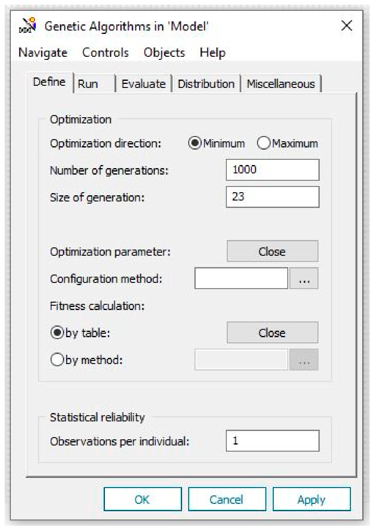
Figure A2.
Applied setting for the number of best individuals in the GAWizard.
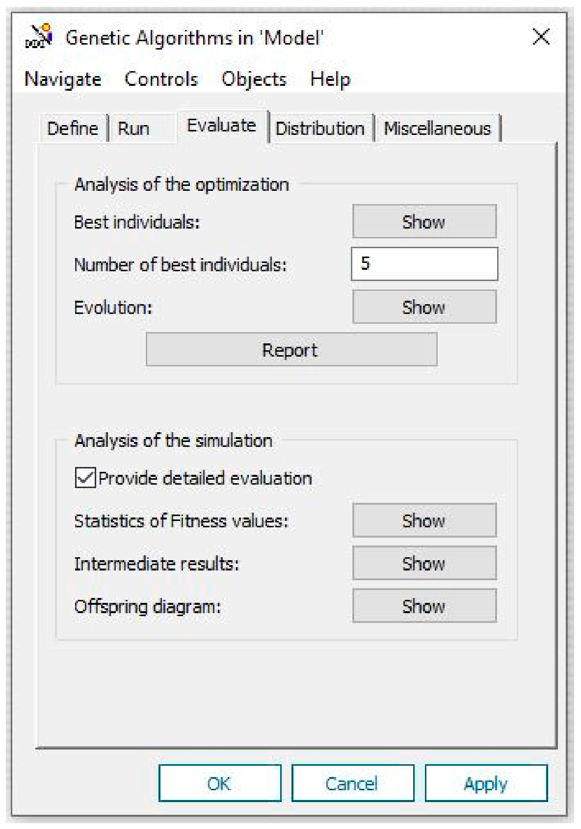
Appendix C
Table A1.
The contents of the FlatProcessTable showing the consecutive manufacturing steps with the stations and the processing times in case of each part type.
References
- Ponsich, A.; Coello, C.C. Differential evolution performances for the solution of mixed-integer constrained process engineering problems. Appl. Soft Comput. 2011, 11, 399–409. [Google Scholar] [CrossRef] [Scilit]
- de Carvalho Miranda, R.; Montevechi, J.A.B.; de Pinho, A.F. Development of an adaptive genetic algorithm for simulation optimization. Acta Sci. Technol. 2015, 37, 321–328. [Google Scholar] [CrossRef] [Scilit]
- Verbiest, F.; Cornelissens, T.; Springael, J. A matheuristic approach for the design of multiproduct batch plants with parallel production lines. Eur. J. Oper. Res. 2019, 273, 933–947. [Google Scholar] [CrossRef] [Scilit]
- Borisenko, A.; Gorlatch, S. Comparing GPU-parallelized metaheuristics to branch-and-bound for batch plants optimization. J. Supercomput. 2019, 75, 7921–7933. [Google Scholar] [CrossRef] [Scilit]
- Borisenko, A.; Gorlatch, S. Efficient GPU-parallelization of batch plants design using metaheuristics with parameter tuning. J. Parallel Distrib. Comput. 2021, 154, 74–81. [Google Scholar] [CrossRef] [Scilit]
- Fei, Y.; Song, M.; Jiao, R.J. AI-assisted Intelligent Discrete-Event Simulation Platform for Manufacturing Systems. In Proceedings of the 15th International Conference on Industrial Engineering and Operations Management, Singapore, 18–20 February 2025; pp. 2748–2759. [Google Scholar]
- Reider, R.; Lang, S. GenAI for Simulation Modeling: A Synergistic Approach. In Proceedings of the 18th International Doctoral Students Workshop on Logistics, Supply Chain and Production Management, Magdeburg, Germany, 17 June 2025; Glistau, E., Ed.; Universitätsbibliothek Magdeburg: Magdeburg, Germany, 2025; pp. 115–122. [Google Scholar] [CrossRef] [PubMed]
- Li, X.; Nassehi, A.; Hu, S.J.; Joung, B.G.; Gao, R.X. A large manufacturing decision model for human-centric decision-making. CIRP Ann. 2025, 74, 621–625. [Google Scholar] [CrossRef] [Scilit]
- Jackson, I.; Jesus Saenz, M.; Ivanov, D. From natural language to simulations: Applying AI to automate simulation modelling of logistics systems. Int. J. Prod. Res. 2024, 62, 1434–1457. [Google Scholar] [CrossRef] [Scilit]
- Frydenlund, E.; Martínez, J.; Padilla, J.J.; Palacio, K.; Shuttleworth, D. Modeler in a box: How can large language models aid in the simulation modeling process? Simulation 2024, 100, 727–749. [Google Scholar] [CrossRef] [Scilit]
- Romero-Guerrero, J.A.; Bautista-Orduna, G.E.; Suarez-Luna, J.M.; Arenas-Islas, D. Creation of discrete event simulation models using artificial intelligence and flexsim. Ing. Investig. Tecnol. 2026, 27, 1–12. [Google Scholar] [CrossRef] [Scilit]
- Elbasheer, M.O.; Laili, Y.; Longo, F.; Solina, V.; Tao, Y.; Veltri, P.; Zhang, Y.; Zhang, L. Natural language-driven production planning: Integrating large language models with automatic simulation model generation in manufacturing systems. J. Intell. Manuf. 2025, 1–28. [Google Scholar] [CrossRef] [Scilit]
- Cirillo, L.; Gotelli, M.; Massei, M.; Sina, X.; Solina, V. A Synergistic Multi-Agent Framework for Resilient and Traceable Operational Scheduling from Unstructured Knowledge. AI 2025, 6, 304. [Google Scholar] [CrossRef] [Scilit]
- Schmitt, T.; Gegenmantel, N.; Moris, M.U.; Mårtensson, P.; Amouzgar, K. LLM-driven discrete-event simulation: A generative AI framework for automated model generation, adaptation, and evaluation in manufacturing. J. Manuf. Syst. 2026, 85, 642–661. [Google Scholar] [CrossRef] [Scilit]
- Korth, M.; Overbeck, L.; Benfer, M.; Lanza, G. LLM-supported Simulation and Exploration in Production Planning and Control. In Proceedings of the ASIM-Fachtagung Simulation in Produktion und Logistik, Dresden, Germany, 24–26 September 2025. [Google Scholar]
- El Baz, H.; Ghali, M.K.; Andrus, L.; Won, D.; Yoon, S.W.; Wang, Y. Generative AI-based optimization for high-mix warehouses: Integrating agentic LLMs and discrete event simulation. Comput. Ind. Eng. 2026, 214, 111884. [Google Scholar] [CrossRef] [Scilit]
- Dehghani, M. SimGPT: Unlocking potentials of generative AI in simulation via Simio and LLM integration. Comput. Ind. Eng. 2026, 218, 112104. [Google Scholar] [CrossRef] [Scilit]
- Alshareef, A. Bootstrapping SysML with LLM-based inference and integrated discrete-event simulation. Simulation 2026, 102, 469–492. [Google Scholar] [CrossRef] [Scilit]
- Kute, S.; Ma, D.; Reider, R.; Müller, M.; Lang, S. Generative AI for Automatic Simulation Model Generation in Factory Planning: A Framework and Prototype. Procedia Comput. Sci. 2025, 274, 1024–1033. [Google Scholar] [CrossRef] [Scilit]
- May, M.C.; Liang, P.; Kim, S.G. Agentic LLM-based Contingency Management in Production Control. Procedia CIRP 2026, 139, 373–378. [Google Scholar] [CrossRef] [Scilit]
- Straka, M.; Ondov, M. Exploring Artificial Intelligence as a Tool for Logistics Process Simulation. Appl. Sci. 2026, 16, 3301. [Google Scholar] [CrossRef] [Scilit]
- Premkumar, L.; Karanjkar, N. On Integrating Resilience and Human Oversight into LLM-Assisted Modeling Workflows for Digital Twins. In Proceedings of the 40th ACM SIGSIM International Conference on Principles of Advanced Discrete Simulation, Vienna, Austria, 24–26 June 2026; pp. 99–115. [Google Scholar]
- Thogaru, H.; Ammanabrolu, P.; Deodhar, A. Warehouse AI: A Closed-Loop Multi-Agent Orchestration for Industrial Planning via Knowledge Graph-Grounded Simulation. Accepted for presentation at the Joint Workshop on Generative AI and Knowledge Graphs (GenAIK 2026) and Knowledge Graphs & Agentic Systems Interplay (NORA 2026), co-located with IJCAI–ECAI 2026, University of Bremen, Germany, 17 August 2026. In press.
- Wagenitz, A.; Toth, M.; Klingebiel, K. Bridging ai-driven risk detection and discrete-event simulation for quantitative supply chain risk evaluation. In Communications of the ECMS; European Council for Modelling and Simulation: London, UK, 2026; Volume 40, pp. 355–361. [Google Scholar]
- Jadhav, P.; Jin, H.; Deelman, E.; Balaprakash, P. Evaluating the Efficacy of LLM-Based Reasoning for Multiobjective HPC Job Scheduling. In Proceedings of the SC ’25 Workshops of the International Conference for High Performance Computing, Networking, Storage and Analysis (SC Workshops ’25), St. Louis, MO, USA, 16–21 November 2025; Association for Computing Machinery: New York, NY, USA, 2025; pp. 2234–2244. [Google Scholar] [CrossRef] [Scilit]
- Miski, A.; Sharif, A.T.; Bukhari, A.G.; Ismail, M. Modeling Discrete-Event Simulations Using Natural Language Processing: A Healthcare Application. J. King Abdulaziz Univ. Med. Sci. 2024, 31, 35. [Google Scholar]
- Diamatopoulos, G.; Theodoropoulos, G.; Tziritas, N.; Bahsoon, R. Towards LLM Augmented Discrete Event Simulation of Blockchain Systems. In Proceedings of the 38th ACM SIGSIM Conference on Principles of Advanced Discrete Simulation, Atlanta, GA, USA, 24–26 June 2024; pp. 75–76. [Google Scholar]
- Katale, T.S.; Gao, L.; Liu, Y.; Liu, D.; Chen, H. LLM-Guided Hybrid Simulation for Airport Cyber-Resilience Assessment. Mathematics 2026, 14, 1923. [Google Scholar] [CrossRef] [Scilit]
- Monks, T.; Harper, A.; Heather, A. Unlocking the potential of past research: Using generative AI to reconstruct healthcare simulation models. J. Oper. Res. Soc. 2026, 77, 1819–1842. [Google Scholar] [CrossRef] [Scilit]
- Mattar, E.A.; Bhattacharya, P.; Dutta, P.K.; Rodrigues, J.J. LLM-FaaS: A Secured Large Language Model assisted Fog-as-a-Service Framework. In 2025 10th International Conference on Smart and Sustainable Technologies (SpliTech); IEEE: New York, NY, USA, 2025; pp. 1–6. [Google Scholar]
- Liu, J.A.; Chu, C.; Zhao, Y.; Aoki, G.; Xiao, Z. Agentic AI for sustainable development: Leveraging large language model-enhanced agent-based modeling for complex policy strategies. Emerg. Media 2025, 3, 401–413. [Google Scholar] [CrossRef] [Scilit]
- Neto, V.V.G.; Keller, N.; Kim, D.D.; Seo, C.; Carbo, P.; Zeigler, B. Preliminary results of an experiment on leveraging large language models to assist modelers in interpreting devs natural language models. In Proceedings of the Workshop em Modelagem e Simulação de Sistemas Intensivos em Software (MSSiS), Curitiba, Brazil, 30 September 2024; pp. 41–50. [Google Scholar]
- Vicente-Martínez, P.; Chust-Ros, A.; Soria-Olivas, E.; García-Escrivà, M.Á.; William-Secin, E.; Sánchez-Montañés, M. A Framework for Conversational Digital Twins: Integrating Generative AI for Operational Event Simulation. Computers 2026, 15, 484. [Google Scholar] [CrossRef] [Scilit]
- Patel, P.; Choukse, E.; Zhang, C.; Shah, A.; Goiri, Í.; Maleki, S.; Bianchini, R. Splitwise: Efficient generative llm inference using phase splitting. In 2024 ACM/IEEE 51st Annual International Symposium on Computer Architecture (ISCA); IEEE: New York, NY, USA, 2024; pp. 118–132. [Google Scholar]
- More, A.; Anwar, T.; Yadav, P. CEDAR: Carbon Efficient Dynamic Allocation and Routing for Agentic LLM Inference. In Proceedings of the 2nd International Workshop on Systems and Methods for Sustainable Large-Scale AI (GreenSys), Edinburgh, UK, 27 April 2026; pp. 25–30. [Google Scholar]
- Jaiswal, S.; Jain, K.; Simmhan, Y.; Parayil, A.; Mallick, A.; Wang, R.; Amant, R.S.; Bansal, C.; Ruhle, V.; Kulkami, A.; et al. SageServe: Optimizing LLM Serving on Cloud Data Centers with Forecast Aware Auto-Scaling. Proc. ACM Meas. Anal. Comput. Syst. 2025, 9, 1–24. [Google Scholar] [CrossRef] [Scilit]
- Zhang, J.; Luo, C.; Su, Z.; Zhang, Q.; Lü, Z.; Ding, J.; Jin, Y. NS4S: Neighborhood search for scheduling problems via large language models. In Proceedings of the Thirty-Fourth International Joint Conference on Artificial Intelligence, Guangzhou, China, 16–22 August 2025; pp. 8687–8695. [Google Scholar]
- Werth, B.; Karder, J.; Beham, A.; Altendorfer, K. Simulation-based optimization of material requirements planning parameters. Procedia Comput. Sci. 2023, 217, 1117–1126. [Google Scholar] [CrossRef] [Scilit]
- Ghaedy-Heidary, E.; Nejati, E.; Ghasemi, A.; Torabi, S.A. A simulation optimization framework to solve stochastic flexible job-shop scheduling problems—Case: Semiconductor manufacturing. Comput. Oper. Res. 2024, 163, 106508. [Google Scholar] [CrossRef] [Scilit]
- Seok, M.G.; Chan, C.W.; Cai, W.; Sarjoughian, H.S.; Park, D. Runtime abstraction-level conversion of discrete-event wafer-fabrication models for simulation acceleration. In Proceedings of the 2020 ACM SIGSIM Conference on Principles of Advanced Discrete Simulation, Miami, FL, USA, 15–17 June 2020; pp. 83–92. [Google Scholar]
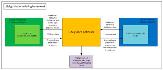
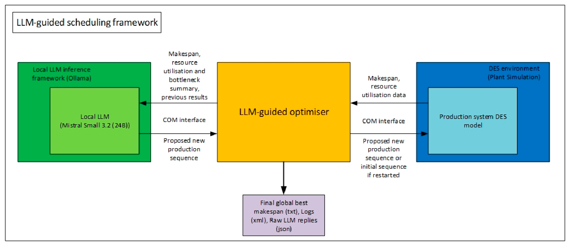
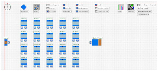
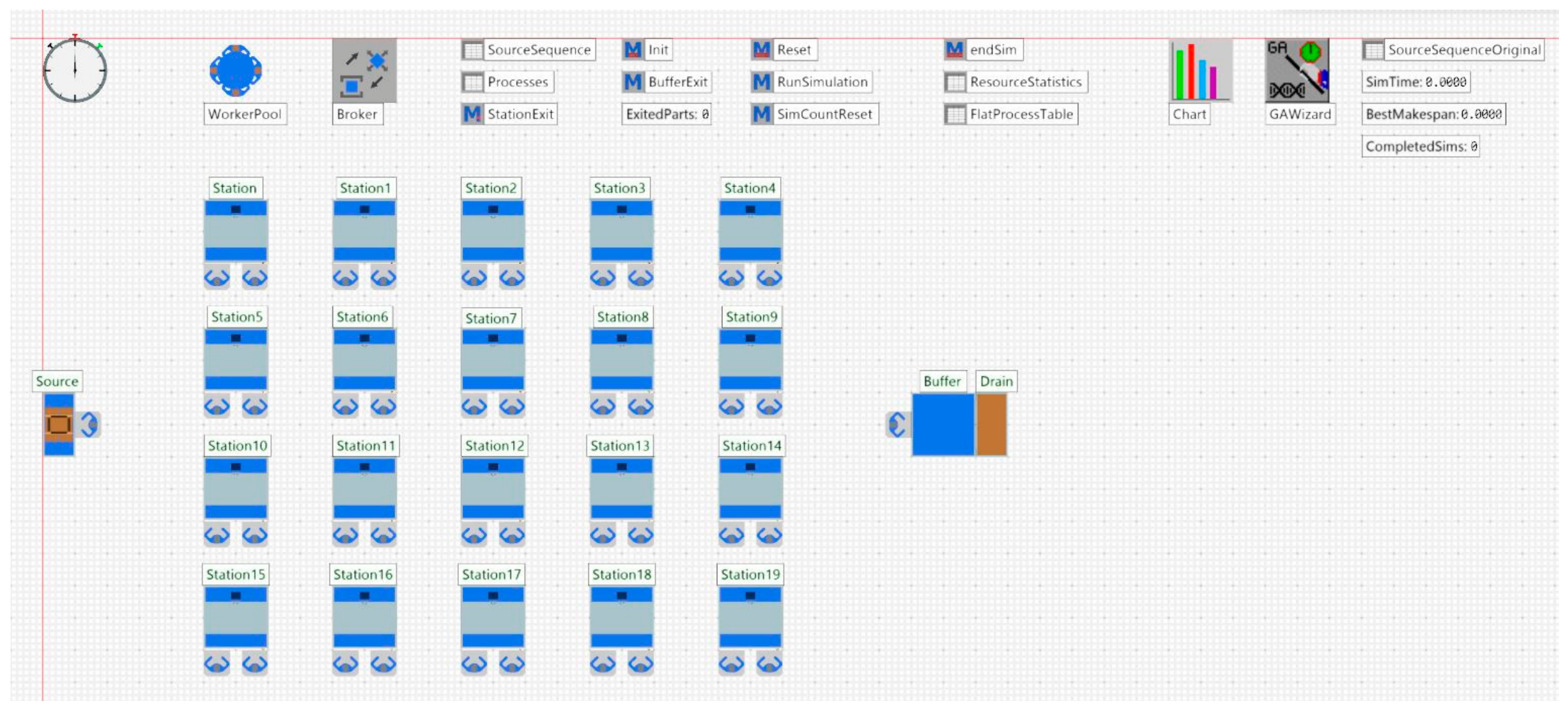
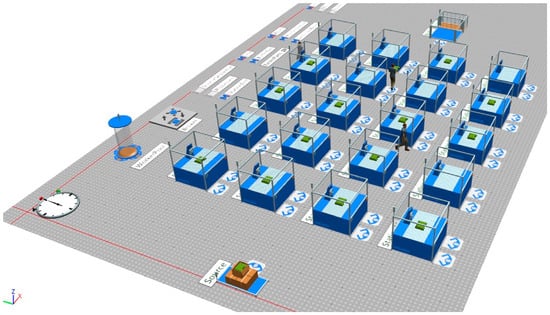
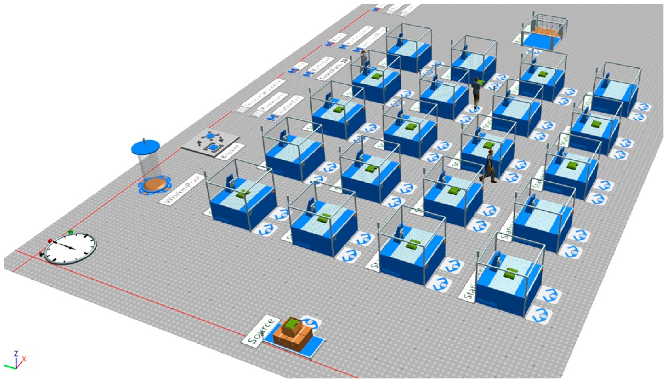
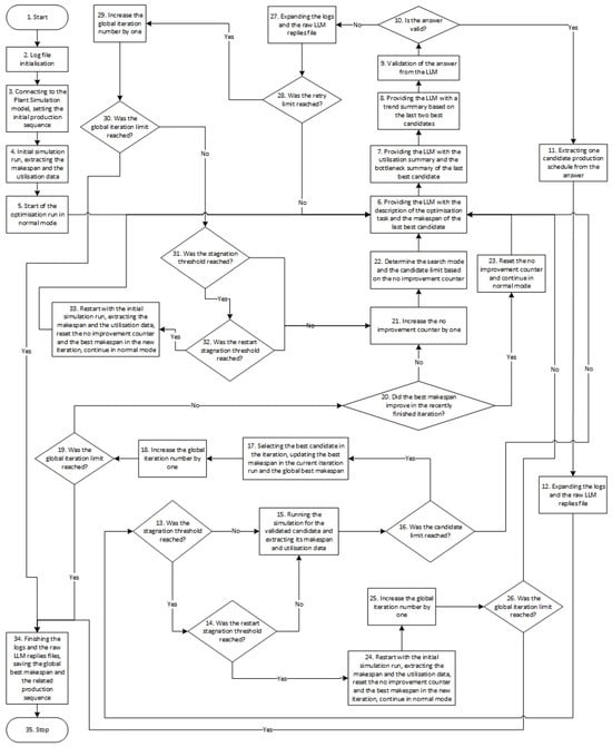
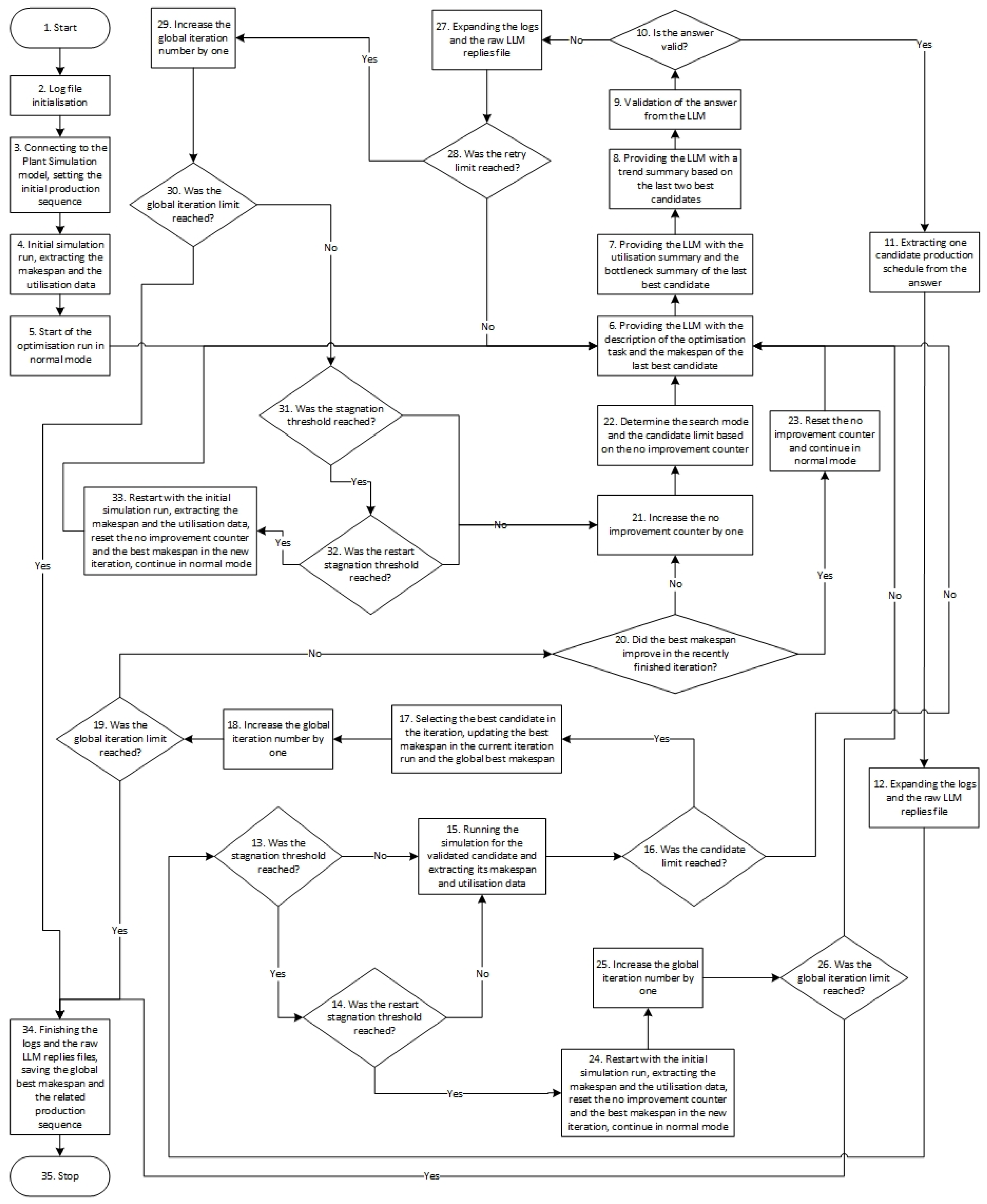
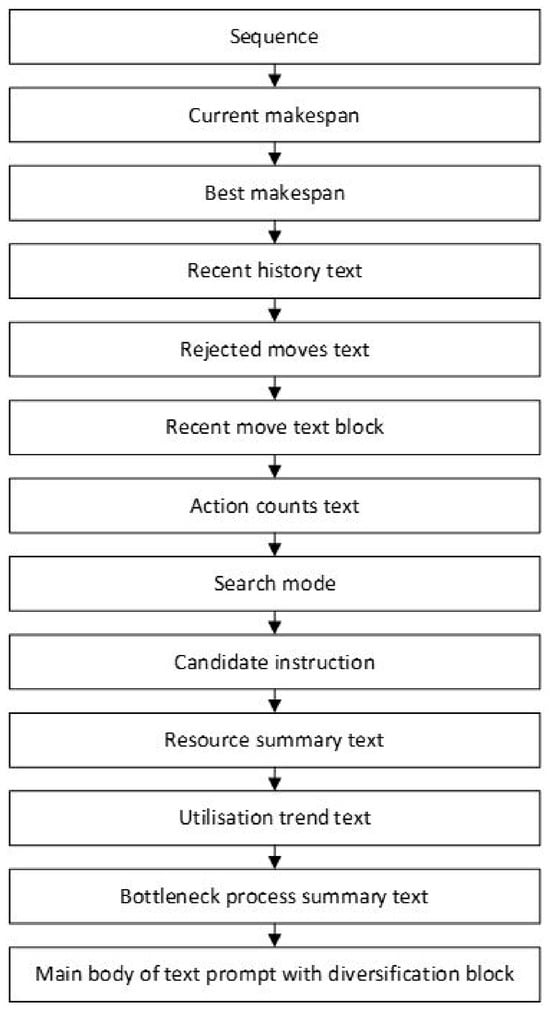
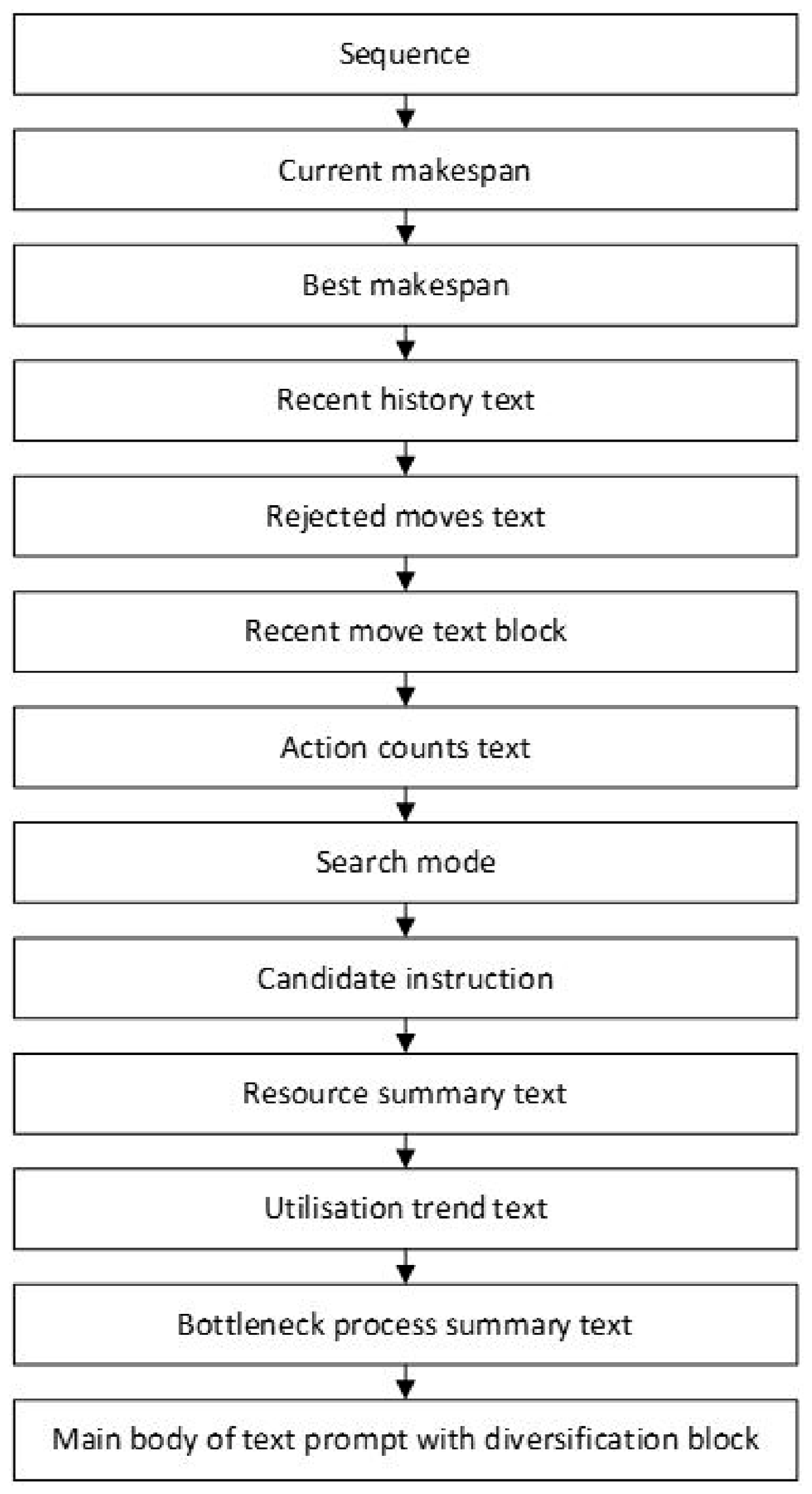
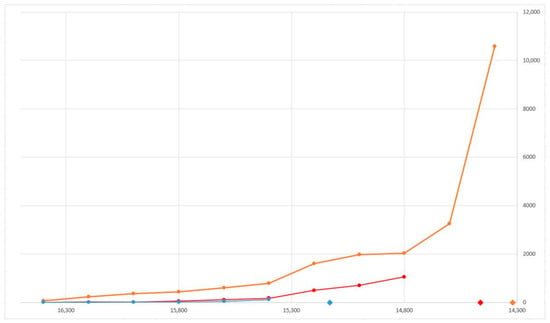
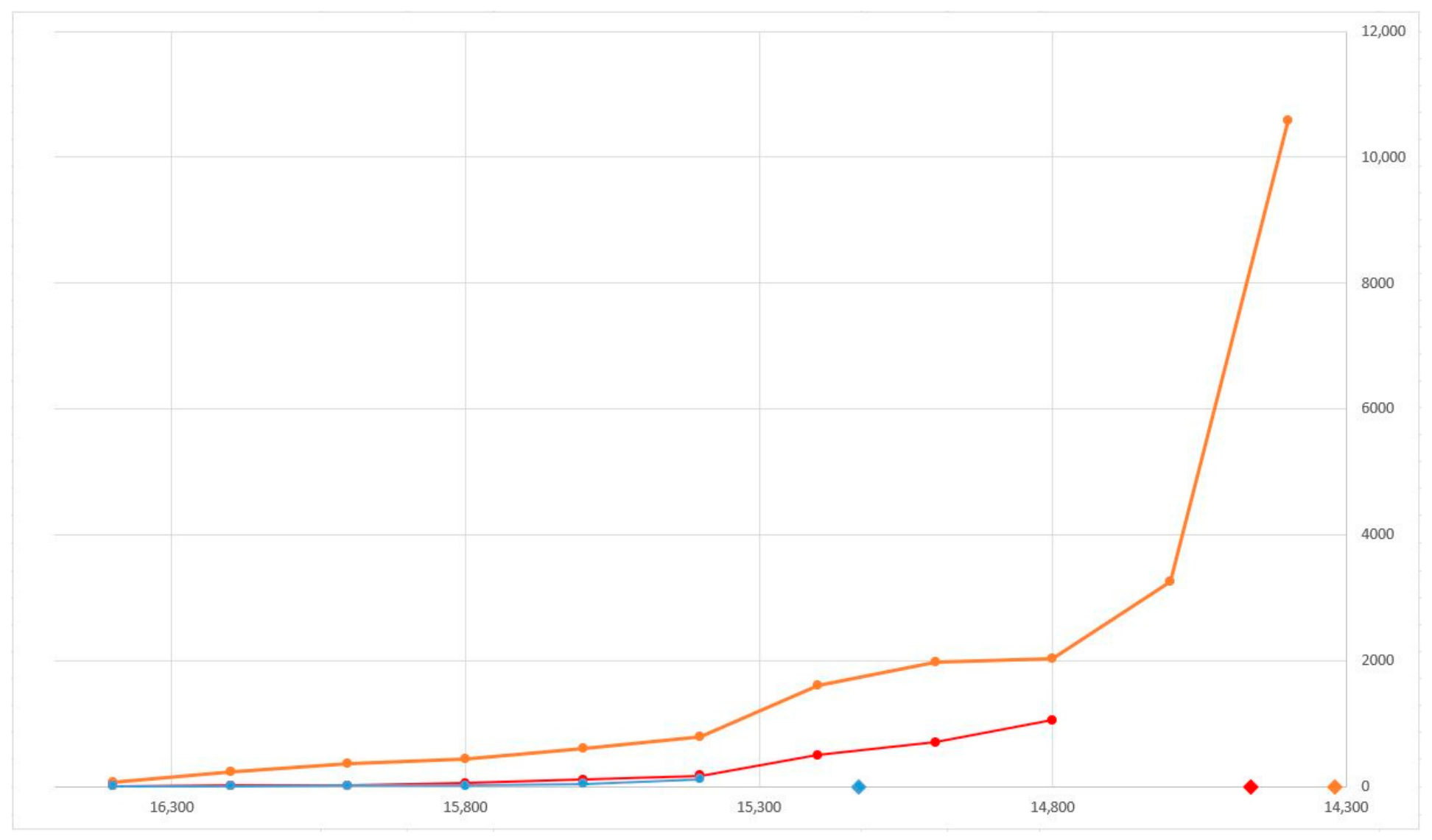
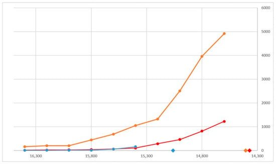
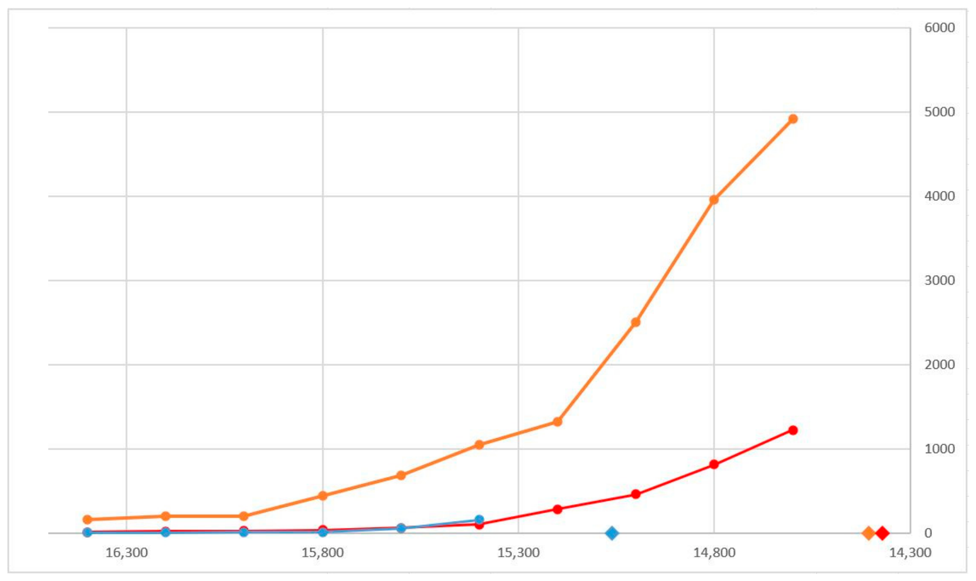
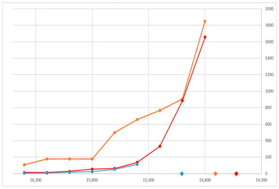
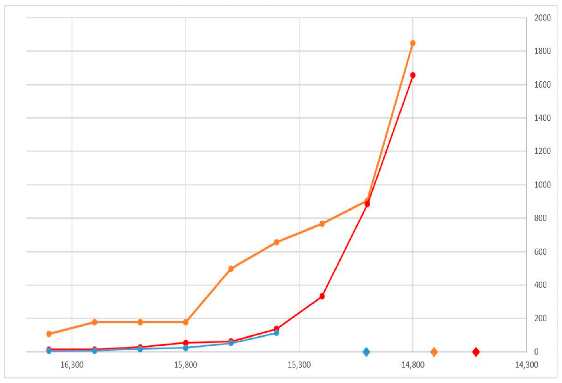

Disclaimer/Publisher’s Note: The statements, opinions and data contained in all publications are solely those of the individual author(s) and contributor(s) and not of MDPI and/or the editor(s). MDPI and/or the editor(s) disclaim responsibility for any injury to people or property resulting from any ideas, methods, instructions or products referred to in the content. |
© 2026 by the author. Licensee MDPI, Basel, Switzerland. This article is an open access article distributed under the terms and conditions of the Creative Commons Attribution (CC BY) license.