


Abstract
The marine capture fisheries sector of the Philippines employs approximately 2.3 million Filipinos, yet recent declines (including a 15.3% drop in Q1 2026 production relative to Q1 2025) underscore the need for forecasting systems resolved at the regional and sectoral level. Existing Philippine approaches rely on univariate classical time-series methods and seldom integrate multivariate oceanographic predictors. This study addresses three questions: (RQ1) How do nine candidate machine learning algorithms compare in forecasting regional fish production from environmental predictors? (RQ2) Which environmental predictors most strongly drive model output, as quantified by explainable AI (XAI) SHAP-based feature attribution? (RQ3) To what extent do model performance and predictor importance vary across regions? Across 32 region–sector panels spanning 2002–2025, kernel and neural network models were selected as the best-performing architecture in 26 of 32 panels (81.3%), achieving a mean composite score 12.7% higher than tree-based ensembles, a gap attributable to extrapolation along trending physical predictors. Feature attribution identified the partial pressure of CO2 as the leading driver in both sectors, exceeding the second-ranked variable by factors of 2.5 (commercial) and 3.4 (marine municipal). Regional heterogeneity in retained predictors, winning algorithms, and SHAP attribution rankings supports region-specific forecasting as a necessary design choice. Mean absolute percentage error of 22–25% and directional accuracy of 0.62–0.66 indicate operational utility for early-warning applications, establishing a basis for evidence-driven priority-setting in Philippine fisheries governance.
1. Introduction
Marine capture fisheries contribute substantially to food security, employment, and coastal livelihoods across the tropical Indo-Pacific, supplying a significant share of animal protein intake among low- and middle-income populations [1,2]. The Philippines consistently ranks among the region’s top fish-producing nations, sustained by both its commercial and municipal fisheries sectors. However, the industry faces notable volatility: the Philippine Statistics Authority [3] reported that total fisheries production in the first quarter of 2026 reached 856,291 metric tons, a 15.3 percent decline from the 1.01 million metric tons recorded during the same period in 2025. The sector employs approximately 2.3 million Filipinos across capture fishing, aquaculture, gleaning, processing, and vending, with nearly half engaged in capture fishing, most of whom operate within municipal waters using small-scale, artisanal methods [4]. Indeed, small-scale fisheries account for more than 85 percent of total wild-caught production nationwide [5]. Given this socioeconomic dependence and recent production declines, forecasting systems that resolve output at the regional and sectoral level are of pressing practical value to fisheries management agencies, food-security planners, and climate-adaptation policymakers.
While overfishing has historically been recognized as the primary driver of declines in fish production, a growing body of evidence indicates that climate-induced environmental change is an increasingly important co-driver of recent trends, often acting synergistically with fishing pressure [6,7,8]. A number of studies indicate that fish stock dynamics in tropical and subtropical seas are jointly modulated by sea surface temperature (SST), ocean acidification indicators such as the partial pressure of CO2 (pCO2) and pH, surface biogeochemistry (chlorophyll-a, dissolved oxygen, nitrate, and phosphate), and physical forcing variables including sea level anomaly, precipitation, and ocean heat content [9,10,11,12,13]. These drivers have been linked to shifts in species distribution, recruitment dynamics, reproductive phenology, and habitat suitability, with cascading effects on the volume and spatial distribution of both commercial and small-scale catches [7,14,15,16]. Characterizing the statistical relationships between such environmental covariates and reported production at the region–sector level can therefore inform management decisions and adaptive planning [17,18], with the caveat that statistical association alone does not establish causal mechanism.
Despite advances in remote sensing, ocean reanalysis products, and machine learning, the integration of these capabilities into fisheries forecasting in the Philippine setting remains uneven [19,20]. Published Philippine forecasting studies have relied predominantly on classical time-series approaches, such as autoregressive integrated moving average (ARIMA) models, seasonal decomposition, and exponential smoothing, usually applied in univariate form and to localized fisheries or aquaculture subsystems [19,21,22]. While extensions such as ARIMAX and vector autoregression can incorporate exogenous predictors, these linear frameworks assume stationarity and additive forcing that may not adequately represent the nonlinear, multi-scale responses characteristic of tropical marine ecosystems [23]. More recent methodological developments have introduced gradient-boosting ensembles, kernel methods, and deep sequential architectures including long short-term memory (LSTM) networks [24], Transformer-based models [25], and Earth-system-oriented deep learning frameworks [26,27] for environmental and ecological time-series forecasting, with growing application to Indo-Pacific pelagic and demersal fisheries [28]. However, comparative evaluations across multiple algorithms remain relatively scarce in the Philippine setting, and existing studies typically focus on one or two regions or a single commodity rather than the full coastal seascape [19,20].
A second consideration in the operational use of machine learning for fisheries governance is interpretability. Complex ensemble and deep learning models can achieve competitive predictive performance, but they are less transparent than classical statistical models, which can limit their uptake by decision-makers who require auditable, defensible outputs [29,30]. SHapley Additive exPlanations (SHAP)—a feature-attribution framework grounded in cooperative game theory—decomposes individual model outputs into additive per-feature contributions and offers a partial response to this concern [31]. SHAP has been applied with increasing frequency in environmental and ecological modeling, including in marine and fisheries contexts such as fishing-ground prediction, species distribution, and habitat suitability [32,33,34,35,36]. However, although multi-algorithm comparative evaluation of machine learning models for fisheries forecasting has expanded in recent years [37,38,39], its combination with SHAP-based attribution in tropical fisheries across a national set of regions and sectors has received comparatively limited attention.
This study develops and evaluates an end-to-end machine learning pipeline for forecasting commercial and marine municipal fish production across the 16 coastal administrative regions of the Philippines for the period 2002–2025. The pipeline integrates ten remote-sensing and reanalysis-derived environmental predictors, a two-step feature-selection procedure that addresses collinearity among carbonate-system and thermal predictors, chronological partitioning with out-of-distribution diagnostics, multi-algorithm comparative evaluation under sequential model-based hyperparameter optimization, composite-score model selection, and SHAP-based per-feature attribution. The study is guided by three research questions:
- RQ1.
- How do nine candidate machine learning algorithms, spanning tree-based ensembles, kernel methods, feedforward networks, and deep sequential architectures, compare in their ability to forecast regional fish production from environmental predictors?
- RQ2.
- Which environmental predictors are most strongly associated with model output for each sector and region, as quantified by SHAP-based feature attribution?
- RQ3.
- To what extent do model performance, retained predictor sets, and feature-importance rankings vary across regions, and what does this variation suggest for the design of region-specific forecasting?
The study describes a reproducible pipeline that combines out-of-distribution diagnostics with composite-score model selection, which may be useful in other short-horizon ecological forecasting tasks where coefficient-of-determination metrics are unstable. It provides a sector-stratified comparative evaluation of nine algorithms applied to Philippine fisheries data across the 16 coastal regions. In addition, it reports the relative importance of environmental predictors and discusses the implications and limitations of these attributions for fisheries monitoring priorities.
2. Methodology
2.1. Research Design
This study adopts a quantitative forecasting design in which sector and region fisheries production is modeled as a function of environmental predictors. The unit of analysis is the (region, sector, time period) cell, and the target variable is total production in metric tons. The commercial and marine municipal sectors are modeled independently to preserve potential asymmetries in environmental coupling, gear restrictions, and reporting mechanisms, all of which are codified in the Philippine Fisheries Code (Republic Act No. 8550, as amended by Republic Act No. 10654) and reflected in the separate statistical reporting pipelines maintained by the Bureau of Fisheries and Aquatic Resources and the Philippine Statistics Authority [3,4,40].
The end-to-end pipeline comprises ten sequential stages: (i) data ingestion from administrative and reanalysis sources; (ii) sectoral and regional aggregation; (iii) data cleaning and imputation; (iv) integration with environmental drivers; (v) two-step feature selection using Spearman’s followed by iterative variance inflation factor (VIF) analysis; (vi) min–max normalization with parameters fitted exclusively on the training partition; (vii) chronological train–validation–test partitioning with out-of-distribution (OOD) diagnostics; (viii) Bayesian (sequential model-based) hyperparameter optimization across nine algorithms; (ix) composite-score evaluation and per-cell winner selection; and (x) SHAP-based explainability analysis of the selected models [31,41].
All pipeline components were implemented in Python 3.11 using scikit-learn 1.4 [42], XGBoost 2.0 [43], LightGBM 4.3 [44], CatBoost 1.2 [45], PyTorch 2.2 [46,47], Optuna 3.6 [48], and SHAP 0.45 [41]. Random seeds were fixed at 42 across all stochastic components—including NumPy, Python’s built-in random module, scikit-learn estimators, and PyTorch’s CPU and CUDA random number generators—to support exact reproducibility.
2.2. Spatial Coverage and Data Sources
This study covers the 16 coastal regions of the Philippines that report marine fisheries landings to the Philippine Statistics Authority (PSA)—the National Capital Region (NCR), the Bangsamoro Autonomous Region in Muslim Mindanao (BARMM), and Regions I–XIII; the landlocked Cordillera Administrative Region (CAR) was excluded. Production data (metric tons) were obtained from the PSA OpenSTAT database, disaggregated into the commercial and marine municipal fisheries sectors, and span 2002–2025 across regions, sectors, and species.
A national bounding box was defined as the outer spatial reference for extracting environmental covariates. Its coordinates were derived from the outermost baseline points of the Philippine Exclusive Economic Zone (EEZ), in accordance with Republic Act No. 9522 and UNCLOS Articles 55–57. The box spans E– E and N– N, providing a buffer around the archipelago [49].
Marine municipal zone. Under RA 10654, municipal fishing waters comprise all marine and inland waters within 15 km of the shoreline and fall under Local Government Unit jurisdiction [50]. For each region served by a BFAR Regional Office, a 15 km coastal buffer was constructed to delineate this zone (Figure 1a). Buffers were derived from the official NAMRIA shoreline vector dataset in the Philippine Reference System of 1992 (PRS92; EPSG:4683) [51] and projected in UTM Zone 51N, the conventional national projection [3].
Figure 1.
Spatial bounding boxes used to delineate the study area: (a) marine municipal fishing zones; (b) commercial fishing zones.
Commercial zone. Commercial fishing grounds extend from 15 km offshore to the outer limit of the EEZ, approximately 370 km (200 nautical miles) from the territorial baselines, as defined under RA 10654. Regional bounding boxes were constructed to capture this offshore extent (Figure 1b) while incorporating relevant ecological and hydrographic conditions.
Ten environmental predictors were assembled from four remote-sensing and reanalysis archives, as shown in Table 1.
Table 1.
Environmental drivers used in the study, with units, source archives, and dataset identifiers.
For each region, all fields were spatially clipped to the regional polygon (encompassing the 15 km municipal water buffer and the broader regional EEZ segment, as appropriate for each variable’s ecological relevance), then aggregated to a single observation value via area-weighted means. Native temporal and spatial resolutions were preserved during clipping; aggregation was performed only after subsetting to the region of interest.
2.3. Data Cleaning and Imputation
Each panel was screened for outliers using Tukey’s interquartile range (IQR) rule [57]. Values below or above were flagged but retained without modification. Retaining rather than removing flagged values reflects current practice in environmental time-series quality control [58,59]: in tropical seas, extreme values frequently reflect genuine geophysical signals associated with El Niño–Southern Oscillation (ENSO) anomalies, typhoon-driven mixing events, and marine heatwaves rather than measurement errors [60,61], and removing them would discard ecologically meaningful information.
Remaining missing values were filled using linear interpolation:
where and are the nearest observed time points. Trailing-edge gaps were filled by backward propagation from the last observed value. Linear interpolation was preferred over spline interpolation and multiple imputation for two reasons: aggregation already smooths sub-seasonal variability, and the bias of linear interpolation grows with gap length and signal curvature, both of which are limited in this dataset [62].
2.4. Feature Selection
A two-step feature selection procedure was applied to the 14 candidate features the 10 environmental predictors at time t and four autoregressive lags of total production at , , , and for each (region, sector) panel, using only the training partition to prevent information leakage [63]. In the first step, a univariate filter retained features whose absolute Spearman rank correlation with total production exceeded and were significant at ; the threshold corresponds to a small but detectable effect size [64] consistent with the sample sizes available at the regional level, while excluding low-signal predictors.
In the second step, an iterative variance inflation factor (VIF) diagnostic was applied to the surviving features. At each iteration, each candidate variable was regressed on the others within the retained set, and the variable with the largest VIF was removed; the process continued until all remaining features satisfied [65]. This threshold was adopted as a pragmatic ecological-modeling convention while acknowledging that no single VIF cut-off is universally appropriate, and that aggressive collinearity-reduction can itself introduce bias [66].
When two candidate variables remained collinear at after VIF filtering, the variable with stronger theoretical or biological grounding was retained over the one with the higher univariate correlation, on the principle that mechanistic interpretability outweighs marginal predictive gain when collinearity structures change across spatial or temporal contexts [67,68].
2.5. Normalization, Chronological Partitioning, and OOD Diagnostics
All retained predictors and the response variable were min–max normalized to the unit interval. To prevent test-set leakage, the normalization parameters were estimated exclusively from the training partition and subsequently reused during validation, testing, and inference; predictions were inverse-transformed back to the metric-ton scale for evaluation [63,69].
Each (region, sector) panel was partitioned chronologically into three sets using an approximate ratio. Over the observation window of 2002 to 2025, this resulted in (2002 Q1–2017 Q4; ≈71%), (2018 Q1–2021 Q4; ≈17%), and (2022 Q1–2025 Q3; ≈12%). Random shuffling was avoided because the production response exhibits strong temporal autocorrelation, and a random split would leak information from future observations into the training set [70].
To diagnose extrapolation behaviour, each observation in and was classified as either in-distribution (normalized value within ) or out-of-distribution (OOD; value or ). An OOD value along a given predictor axis indicates extrapolation beyond the training envelope on that variable. Per-region and per-feature OOD counts and rates were tabulated separately for both sectors.
2.6. Algorithm Suite and Hyperparameter Optimization
Nine algorithms spanning four model families were evaluated for each (region, sector) panel. Their input tensor shapes and tuned hyperparameter spaces are summarized in Table 2.
Table 2.
Machine learning algorithms, input tensor shapes, and hyperparameter search spaces, grouped by model family.
Hyperparameters for each algorithm were optimized using Optuna with the Tree-structured Parzen Estimator (TPE) sampler, a sequential model-based optimization (SMBO) method that approximates Bayesian inference through nonparametric kernel density estimation of high- and low-performing trial configurations [48,71]. Fifty trials were run per (region, sector, algorithm) combination, with validation RMSE on as the objective.
Following optimization, each algorithm was refitted on using its best-trial configuration. Sequential models were trained for up to 100 epochs using the Adam optimizer [72] with mean squared error (MSE) loss on the normalized scale and early stopping based on validation RMSE (patience 10 epochs). The complete experimental design comprised Optuna trials.
2.7. Performance Evaluation and Composite Scoring
Predictive performance was assessed using four regression metrics: mean absolute error (MAE), root-mean-squared error (RMSE), mean absolute percentage error (MAPE), and the coefficient of determination () [73]. On the test set, was computed as , with taken over the held-out window. This formulation can yield negative values whenever a model underperforms the test-set mean, an outcome that is well documented and tends to appear in short held-out windows of small panel time-series [74]. Production scales differ sharply across (region, sector) panels, which complicates direct comparison of error metrics. A composite score was therefore defined to provide a single ranking criterion:
where denotes the range-normalized RMSE and the fractional MAPE; both terms were clipped to . The composite formulation follows established practice for reducing heterogeneous performance criteria to a single ranking index. No individual regression metric is sufficient in isolation: captures explained variance but is unstable over short held-out windows; RMSE quantifies absolute error in production units but is scale-dependent and therefore dominated by high-volume panels; and MAPE expresses scale-free relative error but is unreliable for near-zero observations. Selecting multiple complementary metrics and collapsing them into one scalar to obtain an unambiguous, reproducible winner per panel, is preceded by unified machine-learning evaluation scores such as MLcps [75]. Weight assignment was heuristic: 0.40 to explanatory power and 0.30 each to absolute and percentage error. Truncating at zero via prevents panels with from dragging the ranking downward. The resulting score lies in , where larger values reflect stronger predictive accuracy. For each (region, sector) pair, the model attaining the highest C on was designated the winner.
Two diagnostics were generated for each winning model. The first was a five-axis radar profile showing MAE, RMSE, MAPE (each inverted so that higher readings correspond to better performance), , and C. Every axis was min–max normalized across regions within a sector, which renders cross-region comparison visually tractable. The second diagnostic was a per-region box plot of prediction residuals computed on . Whiskers were drawn at per the Tukey convention [57], and points beyond the whiskers were flagged as residual outliers for case-level inspection of model failures.
2.8. SHAP Explainability
The winning model for each (region, sector) pair was subjected to a SHapley Additive exPlanation (SHAP) analysis [41], a model-agnostic interpretability framework grounded in cooperative game theory. SHAP addresses the interpretability gap that constrains the deployment of complex machine learning models in domains where stakeholders require transparent and accountable decision support [29,30,34]. In fisheries management, where forecasts inform policy decisions affecting livelihoods and food security, attribution-based interpretability is essential for translating black-box predictions into actionable knowledge.
This study adopted the KernelExplainer for all (region, sector) panels. SHAP provides several family-specific implementations—TreeExplainer for tree-based ensembles [31], DeepExplainer for neural networks, and LinearExplainer for linear models that exploit model structure to compute Shapley values more efficiently (and, in the case of TreeExplainer, exactly in polynomial time). However, because the set of winning architectures spans tree-based, kernel, feedforward, and sequential models, using family-specific explainers would yield attributions computed under different approximations and background assumptions, complicating cross-architecture comparison. Therefore, the higher accuracy of TreeExplainer for tree-based models was traded off in favor of a consistent explanation methodology across all panels. KernelExplainer is a model-agnostic, sampling-based approximation that converges to Shapley values as the number of perturbation samples grows [41]; 100 perturbation was used as samples per observation in the experiments, with the training set serving as the background distribution.
SHAP distributes the model prediction among input features according to the additive decomposition [41]:
where is the base value (estimated as the average model output over the training set, computed once and treated as a fixed reference) and is the SHAP value for feature i at input . Each SHAP value is computed using the Shapley formula
where S is any subset of features that does not contain i, F denotes the full feature set, is the model’s prediction when feature i is added to subset S, and is the prediction without i. The marginal contribution measures how feature i alters the prediction when added to subset S, while the combinatorial weight corresponds to the probability of observing S in a uniformly random feature ordering, thereby satisfying the symmetry axiom [76]. Summing across all subsets yields the weighted average marginal contribution of feature i across all possible feature orderings.
Lundberg and Lee [41] prove that the decomposition in Equation (1) is the unique additive feature attribution method satisfying three axiomatic properties: local accuracy (the attributions sum to the difference between the prediction and the base value, ); missingness (features absent from the model receive zero attribution); and consistency (if a model is modified such that a feature’s marginal contribution increases or stays the same across all subsets, its attribution must not decrease). These axiomatic guarantees distinguish SHAP from heuristic feature-importance measures such as gain-based importance in gradient-boosted trees, which are not consistent in this sense [31].
As shown in Figure 2, KernelExplainer samples feature subsets and queries the model to obtain and , then attributes the deviation across the individual features. Each resulting quantifies how much feature i pushed the prediction above or below the base value at observation , with positive values indicating upward contributions and negative values downward contributions. By construction, individual feature impacts sum exactly to the prediction deviation, ensuring a complete and additive decomposition.
Figure 2.
Schematic of the SHAP computation process. The trained model establishes a base value as the average prediction over the training set; KernelExplainer then samples feature subsets and queries the model as a black box, attributing the difference between and across the individual features.
The SHAP attributions, like all post hoc explanations based on input perturbations, can be sensitive to the choice of background distribution and to correlations among features, and have been shown to be vulnerable to adversarial manipulation in classification settings [77]. In the regression context with environmental and autoregressive features, these concerns are mitigated by using the training set as the background distribution (preserving the observed feature correlation structure) and by reporting attributions averaged over rather than for any single observation.
3. Results and Discussion
3.1. Dataset Characteristics
Fisheries production records for 16 coastal regions of the Philippines were obtained from the Philippine Statistics Authority for the period 2002–2025. The dataset comprised 282,783 sectoral records distributed across commercial and marine municipal sectors. Each regional panel contained 11 variables: total production in metric tons (MT) and ten environmental predictors (SST, pCO2, pH, chlorophyll-a, dissolved oxygen, nitrate, phosphate, sea level anomaly, total precipitation, and ocean heat content), yielding 24,576 observations per sector after temporal alignment.
Annual aggregate production trajectories are reported in Figure 3. Commercial production peaked at 1,258,993 MT in 2009 and declined to 851,809 MT by 2025, an 18.5% reduction from the 2002 baseline of 1,045,663 MT. Marine municipal production peaked at 1,184,137 MT in 2010 and declined to 749,367 MT by 2025, a 12.6% reduction from the 2002 baseline of 857,294 MT. Both sectors exhibited sustained declines from 2010 onward, with commercial fisheries declining more steeply.
Figure 3.
Annual fish production (commercial vs. marine municipal).
There are 32 marine species across both sectors, dominated by small and large pelagic species. These include sardines and herrings (e.g., Bali sardinella/tamban, Fimbriated sardines/tunsoy), scads and jacks (Roundscad/galunggong, Big-eyed scad/matangbaka), tunas and tuna-like species (Skipjack/gulyasan, Frigate tuna/tulingan, Yellowfin tuna/ tambakol), Indian and Indo-Pacific mackerels, and anchovies (dilis). Commercial fisheries production is concentrated, with Bali sardinella, Skipjack, Roundscad, Frigate tuna, and Yellowfin tuna contributing approximately 67% of total commercial landings. In contrast, marine municipal fisheries exhibit a more diversified production, with the top five species accounting for only about 42% of total landings, reflecting the gear-diverse and nearshore nature of small-scale fisheries. Sectoral classification followed the two-zone framework established under the Philippine Fisheries Code (Republic Act No. 8550 of 1998, as amended by Republic Act No. 10654 of 2015) [40]. Treating commercial and municipal fisheries as separate modeling units preserves distinctions in fishing grounds, vessel capacity, gear utilization, and reporting systems, while also considering different environmental behavior between offshore and nearshore fisheries [19].
3.2. Outlier Detection and Imputation
The IQR rule flagged values in 9 of 11 variables. The highest rates occurred in the most biologically and physically dynamic fields—phosphate (5.53%), chlorophyll-a (3.48%), and SST (2.93%)—with progressively lower rates for the more slowly varying ones. Notably, neither pH nor produced any flags. This absence is a statistical property of the IQR rule under strongly trending series, not an ecological feature: when a long-term trend dominates total variance [78], the Tukey fences fall outside the observed range and flag no points. The same trend that hides the carbonate variables from outlier detection is what later makes them disproportionately out-of-distribution under chronological partitioning, so the two diagnostics describe a single underlying signal from different angles. Because flagged values were retained rather than removed, the detection rule affects only how extremes are characterized. This is consistent with environmental time-series practice [58,59], in which extreme values in tropical seas usually reflect genuine ENSO, heatwave, and typhoon signals rather than measurement error [60,61].
The temporal clustering of flags supports this geophysical interpretation. The annual outlier budget peaked in 2010, 2014, and 2015, as shown in Figure 4, coinciding with the 2009–2010 and 2015–2016 El Niño events and the onset of the 2014–2016 Pacific marine heatwave [79,80,81], while nutrient-related flags (PO4, NO3, Chl-a) clustered in 2008–2010 and 2017–2018, intervals of intense southwest-monsoon rainfall and cyclone-driven coastal mixing [82]. That the outlier structure tracks known climate anomalies confirms that retention, rather than removal, preserves ecologically meaningful variability.
Figure 4.
Annual outlier counts per environmental variable.
Imputation was minimal and limited to the end of the record. Linear interpolation filled only 0.82% of observations (276 of 33,504), all in , pH, and sea level anomaly during 2025. These gaps reflect publication lag in the OceanSODA-ETHZ [53] and altimetry products, not gaps in the historical data. The longest continuous gap was four quarters, and rates were similar across sectors (0.85% commercial, 0.80% marine municipal). Imputation choice therefore has no meaningful effect on the results.
3.3. Feature Selection: Spearman Correlation and VIF
The univariate Spearman selection was dominated by weak associations of the coefficients reaching significance at (44.4% of 160 in the commercial sector, 49.0% of 157 in the marine municipal sector), and most fell below (137 of 160 and 142 of 157, respectively), with only 9 and 4 classified as strong. That no environmental predictor shows a dominant linear relationship with production is itself informative: it points to multifactorial, likely nonlinear control of regional landings and justifies the multivariate machine-learning approach used here over the univariate classical time-series methods of previous Philippine forecasting studies [19,21,22]. The two leading predictors in both sectors were the carbonate-system variables pH (mean 0.376 commercial, 0.328 marine municipal) and (0.375, 0.312). These formed near-mirror pairs within individual regions—for example, ranging from () to (pH) in commercial Region VII (Central Visayas), and from (pH) to () in marine municipal BARMM (Figure 5). This mirroring is the expected thermodynamic signature of the seawater carbonate equilibrium, not a data artifact, and it foreshadows the collinearity that the second selection step was designed to resolve.
Figure 5.
Correlation heatmaps of the predictor variables: (a) commercial fisheries; (b) marine municipal fisheries.
The iterative VIF procedure reduced all retained features to , with only four cells per sector entering the caution band. Two collinear structures recurred across nearly all regions: pH– (median ; 16/16 commercial and 14/16 marine municipal regions) and SST–OHC (; 16/16 regions in both sectors), as shown in Figure 6. Both are physically expected—the first from carbonate chemistry, the second because ocean heat content integrates temperature through the water column—so consolidating each pair removes redundancy without discarding distinct ecological information. Where a pair remained collinear, the variable with stronger mechanistic grounding ( over pH, SST over OHC) was retained in preference to the one with marginally higher univariate correlation, consistent with the principle that interpretability should outweigh small predictive gains when collinearity structure varies across space [67,68].
Figure 6.
Variance inflation factor (VIF) heatmaps of the predictor variables: (a) commercial fisheries; (b) marine municipal fisheries.
The retained-predictor sets differed systematically between sectors, and this divergence is the key scientific outcome of the selection stage. Commercial panels most often retained thermal–acidification predictors (SST, , sea level anomaly, with ocean heat content also prominent in the univariate ranking), whereas marine municipal panels favoured hydrological–nutrient predictors (rainfall, sea level anomaly, , and phosphate), with SST holding the lowest univariate rank in that sector (Figure 6). This contrast—recovered here by a purely linear, model-free screen mirrors the spatial ecology of the two fishing zones: offshore commercial grounds are coupled to the integrated thermal and carbonate state of the open mixed layer, while nearshore municipal grounds also respond to runoff-mediated nutrient delivery.
3.4. Out-of-Distribution Diagnostics
Roughly one in nine held-out observations fell outside the training envelope in each sector (11.4% commercial, 11.0% marine municipal), and in both cases the burden was concentrated on the test fold rather than the validation fold (test-set OOD rates of 7.1% and 6.9%, versus 4.3% and 4.2% on validation). This concentration is a direct consequence of chronological partitioning: because the held-out window is the most recent in time, it sits furthest along the secular trends in the strongest physical predictors— exceeded 22% OOD in both sectors and sea level anomaly approached 20% in the marine municipal panels (Appendix A). The distribution shift is therefore not a sampling accident but an intrinsic feature of forecasting monotonically trending environmental drivers into an unobserved regime, and it cannot be removed by model choice or by reshuffling the data without leaking future information into training.
3.5. Comparative ML Algorithm Per-Region Performance
The algorithm ranking by mean validation RMSE was remarkably consistent across sectors: smooth-output learners (MLP, SVR, and the recurrent and attention-based networks) occupied the top tier, while the four tree-based ensembles clustered at the bottom, trailing the best learner by 34.4% in mean validation error (Figure 7). The two sectors differed only in the internal ordering of the leading group, with the recurrent architectures exchanging rank. The Optuna best-trial index clustered in the middle to late portion of the 50-trial search, with several models locating their best configuration as late as trial 49 (Appendix B).
Figure 7.
Optuna hyperparameter tuning.
This margin reflects a structural property of the predictor space rather than a generic advantage of neural architectures—a distinction central to interpreting the result correctly. Three of the strongest retained predictors (, sea level anomaly, SST) trend monotonically across 2002–2025, and chronological partitioning placed much of the test fold beyond the upper training envelope on these variables ( exceeded 22% OOD in both sectors, and sea level anomaly approached 20% in the marine municipal sector). Tree-based learners produce piecewise-constant predictions bounded by training-set extremes and so cannot extrapolate along monotonic trajectories, whereas the MLP, RBF-SVR, and recurrent and attention-based architectures keep smooth response surfaces beyond the training range and remain functional under extrapolation. The implication for environmental machine learning is methodological and generalizable: where predictors trend and the held-out window is defined chronologically, model-family selection must be governed by the geometry of the predictor space relative to that window, not by aggregate validation metrics alone. This contrasts with the common practice in ecological forecasting of selecting a single algorithm on pooled or randomly partitioned data [37,38,39], which can mask exactly the extrapolation failure that dominates here.
In the commercial sector, validation-stage winners were dispersed across eight architectures, and tree ensembles still led several regions by mean validation RMSE; in the marine municipal sector the distribution concentrated on the smooth learners (MLP, LSTM, Transformer), and no tree-based ensemble led the validation-RMSE ranking in any region. That no single algorithm exceeded 5 of 16 regions in either sector indicates that regional production dynamics in the Philippine archipelago are not reducible to one forcing structure.
3.6. Performance of the Selected Best Models and Regional Heterogeneity
The selected models achieved mean composite scores of 0.543 (commercial) and 0.515 (marine municipal), with mean test MAPE of 24.84% and 22.88% respectively (per-region metrics in Table 3, winning hyperparameters in Table 4). The most consequential figure is the change in cross-regional mean test : per-region selection moved the commercial sector from under any single pooled algorithm to , and the marine municipal sector from to . This is the quantitative payoff of regionalization per-region selection recovers substantive predictive signal that is invisible to a globally pooled estimator. The smaller absolute gain in the marine municipal sector reflects its heavier out-of-distribution burden in nearshore panels rather than a failure of the approach; in proportional terms the improvement is comparable.
Table 3.
Selected best model per region and sector, with test-set metrics.
Table 4.
Optuna-tuned hyperparameters of the winning algorithm for each region–sector panel.
The range of fits is wide and geographically interpretable, which is itself a substantive finding rather than a caveat. The strongest fits in both sectors—Region IX (Zamboanga Peninsula) and Region II (Cagayan Valley), each an MLP—fall within the “highly accurate” band conventionally defined by MAPE [83], confirming that the methodology produces operationally actionable forecasts under favourable forcing. The weakest fits both occurred in Region V (Bicol), where even the best of nine candidates underperformed a constant-mean baseline (). These extremes track the oceanography: Region IX borders the upwelling-influenced Sulu Sea under a relatively stable seasonal regime, whereas Region V faces the Pacific seaboard and is repeatedly disturbed by tropical cyclones, ENSO thermal anomalies, and monsoon transitions whose interacting structure exceeds what a 50-trial search can resolve from a 24-year quarterly record. That model skill rises and falls with the predictability of the local forcing regime—rather than with data volume alone—is consistent with descriptions of the Philippine seascape as a mosaic of distinct oceanographic provinces rather than a homogeneous tropical system. It also means “best model” in low-skill regions should be read as relative within the candidate set, not as evidence of acceptable fit.
A recurring metric divergence reinforces why composite scoring, rather than any single criterion, was used for selection. In Region II, a high (0.745) coincides with a high MAPE (46.30%) because MAPE inflates when actual production values are small; relying on either metric alone would have produced misleading rankings, whereas the composite score weights , RMSE, and MAPE jointly and smooths over such disagreements.
The distribution of winning architectures carries the central argument of this study. Winners dispersed across at least six architectures in each sector, with no algorithm exceeding 5 of 16 regions, indicating that regional production dynamics across the archipelago are not reducible to a single forcing structure. The clearest sectoral contrast is in the fate of tree-based ensembles, which collectively won 5 of 16 commercial regions but only a single marine municipal region. Combined across both sectors, kernel and neural network models were selected as the best-performing architecture in 26 of 32 panels (81.3%), achieving a mean composite score 12.7% higher than tree-based ensembles (0.54 vs. 0.48). Two mechanisms plausibly explain this asymmetry. First, tree learners cannot extrapolate beyond the training range, and the strongest marine municipal predictors carry a comparable or heavier held-out OOD burden ( 22.7%, sea level anomaly 19.5%) than their commercial counterparts (26.8% and 17.0%), penalizing non-extrapolating models where the test fold escapes training extremes. Second, the marine municipal sector leans more on nutrient and freshwater predictors (rainfall, nitrate, phosphate) whose shorter-term fluctuations are captured more effectively by architectures with temporal inductive biases MLP with engineered lags, and the recurrent and attention-based networks than by tree splits on raw values.
Taken together, these results argue against a globally pooled estimator for Philippine fisheries forecasting and establish per-region model selection as a necessary design choice. Pending local validation, an ensemble of the top three neural architectures (MLP, LSTM, Transformer) is a defensible default for any new region.
3.7. Residual Diagnostics
Residuals () were examined for each region on the pooled held-out period . Across both sectors the residual distributions were near-centred—cross-regional mean residual medians of MT (commercial) and MT (marine municipal)—indicating only a slight systematic tendency to over-predict and no large directional bias once models were selected per region (Figure 8 and Figure 9). Residual outliers were infrequent and comparable between sectors (1.5 and 1.7 per region), so the level of fit is not propped up by a few well-behaved regions while others fail catastrophically; the modest spread is distributed broadly.
Figure 8.
Residual distribution (commercial fisheries).
Figure 9.
Residual distribution (marine municipal fisheries).
The more informative pattern is that residual spread scaled with regional production volume strongly in the commercial sector (Spearman , ) and moderately in the marine municipal sector (Spearman , ). This is the expected signature of multiplicative rather than additive error: absolute uncertainty grows with the quantity being predicted, while relative uncertainty remains roughly constant across regions of very different scale. The weaker association in the marine municipal sector is itself interpretable, reflecting the gear-diverse, nearshore character of small-scale fisheries, where local nutrient and freshwater forcing introduces error components not tied to production volume. In practical terms, this scaling explains why MAPE is the more comparable accuracy metric across regions spanning an order of magnitude in output, and justifies its inclusion alongside RMSE in the composite score.
3.8. Operational Validation
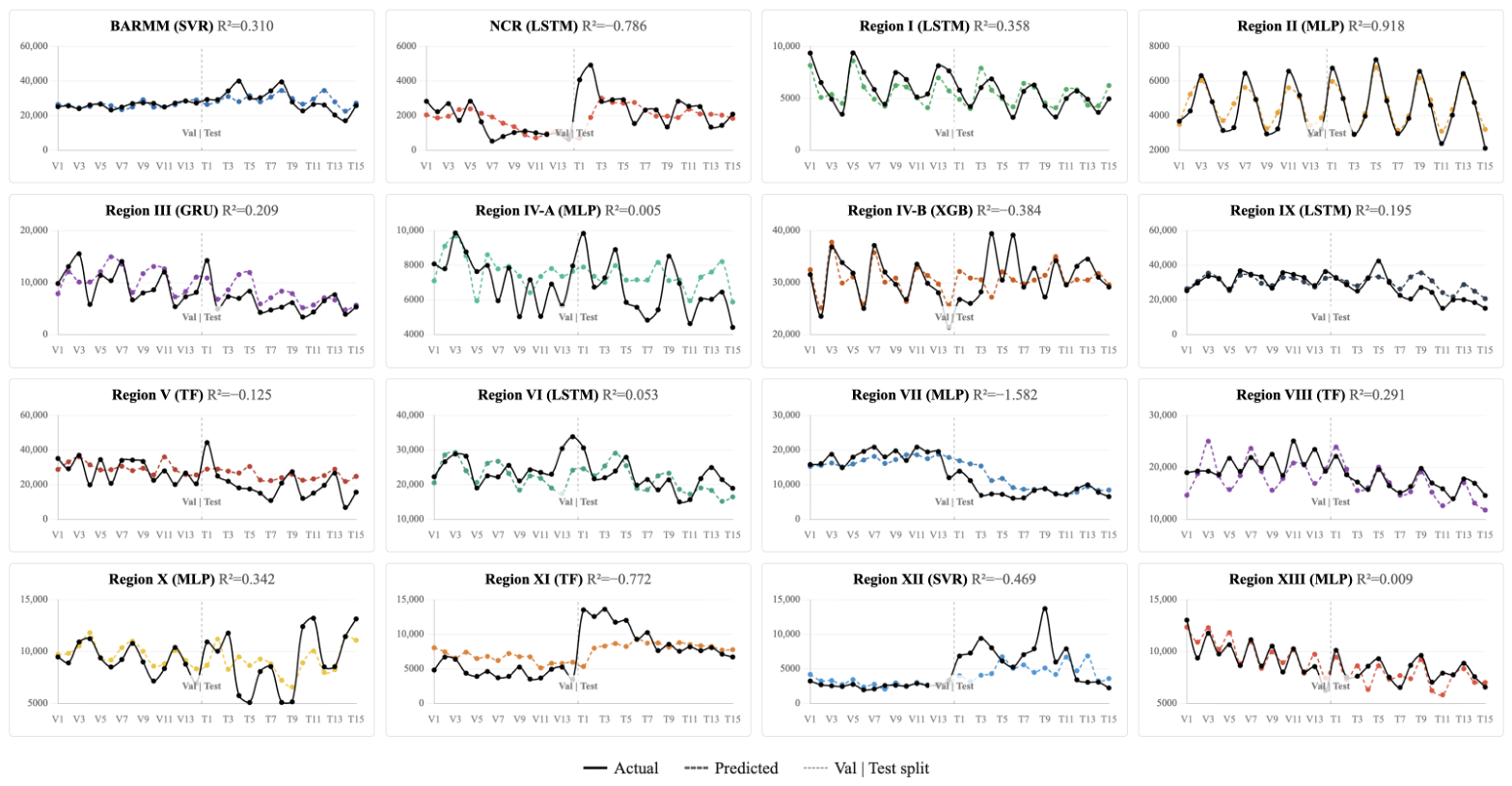
Predicted-versus-actual traces for each region’s selected model (Figure 10; circles , triangles , dashed line ) show a consistent but modest degradation from validation to test, with cross-regional mean MAE ratios near 1.8 in both sectors. The much lower medians (1.07 and 1.27) reveal that this mean is inflated by a handful of regions—BARMM in both sectors, and Regions X, XII, IV-B, and IX—where validation MAE was anomalously small rather than test MAE anomalously large. The typical region therefore generalises far better than the mean ratio implies, and the degradation reflects a few favourable validation folds rather than systematic overfitting.
Figure 10.
Actual vs. predicted production for each region’s selected best model: (a) commercial fisheries; (b) marine municipal fisheries.
Directional accuracy is the more operationally relevant diagnostic, and the forecasts perform better on it than the level-error metrics alone would suggest: mean test directional accuracy was 0.621 (commercial) and 0.656 (marine municipal), both well above the 0.5 baseline. The traces fall into three interpretable patterns (Appendix C)—tight overlay with symmetric residuals in well-forced regions (e.g., Region IX, NCR, Region II); amplitude attenuation, in which the model tracks central tendency but flattens peaks; and near-zero or anti-phase behaviour confined to the small set of regions whose forcing the models cannot resolve. This gradient maps onto the oceanographic heterogeneity identified throughout the analysis: the regions of tight overlay are those under stable seasonal forcing, while the anti-phase cases concentrate in regions exposed to irregular cyclone- and ENSO-driven perturbation.
Two failure modes merit separation because they imply different remedies. In Region IV-A (commercial), a phase-misalignment failure produces plausible amplitude but inverts the direction of change on most consecutive periods—a timing error that additional lag structure or spatial information might correct. In Region V (marine municipal), a level-offset failure does the opposite: the model tracks direction correctly on 6 of 7 test periods yet sits systematically above the actual series, producing the largest MAPE in the comparison a calibration error that bias-correction or uncertainty-aware post-processing could mitigate. Distinguishing the two clarifies that low aggregate accuracy in a region does not always mean the model has learned nothing; it may have learned timing but not level, or level but not timing.
That directional accuracy exceeds 0.62 in both sectors despite mean test MAPE of 22–25% is the result that establishes operational utility. For early-warning use, the sign of period-to-period change—whether production is likely to rise or fall is more actionable than its exact magnitude, and the forecasts carry that information reliably even where absolute level prediction is imperfect. The framework is therefore usable for management in its present form, before the upper bound of absolute accuracy is reached.
3.9. SHAP Explainability and Environmental Drivers
Per-region feature importance was computed as the lag-averaged mean value and aggregated across regions, as shown in Figure 11. The central finding is unambiguous and consistent across sectors: was the leading attributed driver of model output, exceeding the second-ranked predictor by a factor of 2.5 in the commercial sector and 3.4 in the marine municipal sector. This ranking reflects environmental predictors only; at the level of individual predictions, autoregressive lag terms remain the single largest contributor overall, ahead of any environmental feature in most regions (Appendix D), consistent with production forecasting being anchored primarily by recent history and modulated secondarily by environmental forcing. This is the most operationally consequential result of the study, because it identifies carbonate chemistry—rather than the more routinely monitored temperature and chlorophyll fields—as the dominant predictor the models exploit. The result is consistent with a substantial body of evidence that ocean acidification exerts first-order effects on tropical marine ecosystems, impairing calcification, larval recruitment, and sensory and behavioral function in fishes, with cascading consequences for community structure [10,11]. It is also structurally consistent with the carbonate collinearity resolved earlier (pH– median . The retained signal carries the integrated carbonate-system information that the VIF procedure consolidated from the original pair, so its SHAP dominance reflects the whole carbonate system rather than CO2 partial pressure alone.
Figure 11.
Global feature importance commercial and marine municipal fisheries.
The secondary tier of drivers diverged systematically between sectors, and this divergence not the values themselves is the interpretively important result. Commercial panels were dominated by thermal–acidification predictors (SST, sea level anomaly), whereas marine municipal panels gave greater weight to nutrient–hydrological predictors, with rainfall and phosphate entering the top five roughly twice as often as in commercial panels, as shown in Figure 12. Region-level SHAP dependence plots (Appendix E) confirm that this heterogeneity extends beyond ranked importance to the underlying feature–output relationships themselves: per-region slopes frequently change sign across regions for the same predictor, so pooled trends remain shallow ( for most features in both sectors). Dissolved oxygen was the least influential feature in both sectors. This pattern mirrors the spatial ecology of the two fishing zones: offshore commercial grounds respond primarily to the integrated thermal and carbonate state of the open mixed layer, where pelagic distribution and abundance follow basin-scale temperature and chemistry, while nearshore municipal grounds respond additionally to runoff-mediated nutrient delivery at the land–sea interface, where rainfall and river discharge regulate coastal productivity. That a model-agnostic, post hoc attribution method recovers this offshore–nearshore partitioning independently after it had already emerged from the linear feature-selection screen is strong internal evidence that the sectoral contrast is an ecological signal rather than a modeling artifact.
Figure 12.
SHAP feature importance: (a) commercial fisheries; (b) marine municipal fisheries.
These attributions should be read with appropriate caution. SHAP quantifies each feature’s contribution to model output, not to the production process itself, and the strength of the attribution is partly inflated by its role as the smoothest, most monotonically trending retained predictor: in regions where the test fold extrapolates along , the model necessarily leans on it to track the trajectory, and the SHAP magnitude reflects that reliance. However, three independent lines of evidence converge on the carbonate system the near-mirror pH/ univariate correlations in every region, the OOD-driven loss of non-extrapolating tree learners in the marine municipal sector, and the SHAP attribution here providing triangulated support that carries genuine and substantial predictive signal, not merely an extrapolation proxy. This convergence across methodologically independent diagnostics is what licenses the operational recommendation to prioritize carbonate-system monitoring.
3.10. Limitations
Several limitations qualify these findings and define the conditions under which the forecasts should be interpreted.
Out-of-distribution observations and distribution shift. Chronological partitioning placed 11.0–11.4% of held-out observations beyond the training envelope, rising above 22% for and approaching 20% for sea level anomaly on the strongest physical predictors. This distribution shift is intrinsic to forecasting monotonically trending environmental variables and is the principal driver of both the algorithm-family ranking and the negative cross-regional test values reported here. It cannot be removed by model choice alone; it reflects the genuine difficulty of forecasting fisheries production into an environmental regime not previously observed.
Model uncertainty. The reliance on a single fixed chronological train–validation–test split, adopted to respect temporal autocorrelation, precludes resampling-based uncertainty quantification and limits the formal statistical inference that can be drawn from cross-regional performance comparisons. The forecasts reported here are point estimates without predictive intervals, and the wide cross-regional dispersion of test (from strongly positive to low ) should be read as evidence that forecast reliability itself varies markedly by region.
Limitations of the modeling and explanability framework. The 50-trial Optuna budget, although adequate for locating competitive configurations, clustered best-trial indices in the middle-to-late portion of the search, suggesting incremental gains may remain available under a wider hyperparameter space. The KernelExplainer, adopted to enable consistent cross-architecture SHAP comparison, trades the exactness of TreeExplainer for tree-based models and the structural efficiency of DeepExplainer for neural networks; family-specific explainers would yield slightly different attribution magnitudes, although the ranking structure is unlikely to change. Finally, SHAP quantifies each feature’s contribution to model output, not to the underlying production process: the prominence of is partly inflated by its position as the smoothest, most monotonically trending retained predictor, so the attributions should be read as statements about model behavior under extrapolation rather than as direct evidence of ecological causation.
3.11. Future Research Directions
This work suggests several avenues for extension. First, the regional heterogeneity documented here motivates explicitly spatial models: a spatiotemporal graph neural network layer (for example GAT-LSTM, GAT-GRU, or a Graph Transformer) operating over a regional adjacency graph defined by shared marine ecoregions or hydrographic connectivity could allow information to propagate between oceanographically linked regions and improve forecasts in data-poor panels where single-region models underfit.
Second, the predictor set could be broadened to include ocean-current velocity, mixed-layer depth, eddy kinetic energy, and basin-scale climate indices (ENSO, PDO, IOD), together with fishing-effort proxies derived from vessel-tracking (AIS) data, which would help disentangle environmental forcing from harvesting pressure—a confound the present production-only target cannot resolve.
Third, advanced ensemble strategies such as stacked generalization or Bayesian model averaging across the top neural architectures (MLP, LSTM, Transformer) may yield more robust forecasts than per-region winner selection, particularly for regions near the no-skill baseline.
Fourth, the point forecasts reported here should be augmented with calibrated uncertainty quantification; conformal-prediction methods designed for non-exchangeable and distribution-shifted time series are well suited to the out-of-distribution conditions documented in this study and would yield prediction intervals with finite-sample coverage guarantees.
Finally, the pipeline is transferable: applying it to other Indo-Pacific small-scale fisheries, and coupling its outputs to stock-assessment and bio-economic models, would situate the environmental forecasts within the decision frameworks actually used in fisheries management.
4. Conclusions
This study developed and evaluated an end-to-end, explainable machine learning pipeline for forecasting commercial and marine municipal fish production across the 16 coastal regions of the Philippines over 2002–2025. The framework integrated ten remote-sensing and reanalysis-derived environmental predictors, two-step feature selection, out-of-distribution (OOD) diagnostics, Bayesian hyperparameter optimization across nine algorithms, composite-score model selection, and SHAP-based attribution. Across 32 region–sector panels it produced operationally deployable forecasts, with a held-out mean absolute percentage error of 22–25% that is competitive with published small-pelagic forecasting accuracies in the Indo-Pacific.
Three principal findings emerged. First, kernel and neural network models were selected as the best-performing architecture in 26 of 32 region–sector panels (81.3%), achieving a mean composite score 12.7% higher than tree-based ensembles, reflecting the inability of piecewise-constant predictors to extrapolate along trending physical drivers such as pCO2, sea level anomaly, and SST. Tree-based ensembles won only a single marine municipal region (Region IV-B) out of 16 at final selection. Second, SHAP attribution identified pCO2 as the dominant driver of production variability in both sectors, exceeding the second-ranked predictor by a factor of 2.5 (commercial) to 3.4 (marine municipal), with secondary drivers differing by sector in a manner consistent with the spatial ecology of offshore versus nearshore grounds. Third, substantial regional heterogeneity in retained predictors, winning algorithms, and SHAP rankings recovered known oceanographic regime differences across the Philippine seascape, supporting a region-specific rather than a globally pooled forecasting strategy.
This work makes three contributions. Methodologically, it presents the first national-scale, sector-stratified forecasting pipeline for Philippine marine fisheries to combine multi-algorithm comparison, OOD diagnostics, composite-score selection, and SHAP attribution in a single reproducible workflow, demonstrating that model-family selection must be governed by the geometry of the predictor space relative to the held-out window rather than by aggregate validation metrics. Scientifically, the convergent identification of the carbonate system as the dominant driver—triangulated across Spearman correlation, OOD-driven selection, and SHAP—supports elevating carbonate-system monitoring to a first-order operational priority alongside existing SST and chlorophyll-a infrastructure. For management, region-specific predictor sets and winning algorithms, together with above-baseline directional accuracy (greater than 0.62 in both sectors), argue against uniform national policy levers and in favor of a regionalized, evidence-driven approach to quota setting, closed-season design, and fleet-capacity management.
Several limitations should be noted. The predictors rely on remote-sensing and reanalysis proxies rather than in situ carbonate measurements, and fishing effort and socioeconomic covariates were not explicitly modeled, leaving scope for omitted-variable confounding. Future work should integrate effort and socioeconomic predictors, validate the attributed carbonate signal against in-situ observations, and extend the pipeline toward operational deployment for fisheries early warning. Overall, these findings establish that environmental predictors particularly the carbonate system carry substantial and interpretable predictive signal for Philippine fisheries production and that an explainable machine learning pipeline can deliver forecasts of operational utility while remaining transparent and auditable for fisheries governance.
Author Contributions
Conceptualization, P.B.J., K.J. and M.J.; methodology, P.B.J., K.J. and M.J.; software, P.B.J.; validation, P.B.J., K.J. and M.J.; formal analysis, P.B.J., K.J. and M.J.; investigation, P.B.J.; resources, P.B.J., K.J. and M.J.; data curation, P.B.J.; writing—original draft preparation, P.B.J., K.J. and M.J.; writing—review and editing, P.B.J., K.J. and M.J.; visualization, P.B.J.; supervision, K.J. and M.J.; project administration, K.J. and M.J.; funding acquisition, P.B.J., K.J. and M.J. All authors have read and agreed to the published version of the manuscript.
Funding
This research was funded by Walailak University through the Graduate Scholarship Program.
Data Availability Statement
The original contributions presented in this study are included in the article. Further inquiries can be directed to the corresponding author.
Acknowledgments
The support provided through the Walailak University Graduate Scholarship Program played a significant role in the successful completion of this research and the achievement of its objectives. The authors sincerely acknowledge Walailak University for its continued commitment to advancing research and academic excellence. In the preparation of this manuscript, ChatGPT (GPT-5.5) was utilized exclusively for language paraphrasing to enhance clarity and coherence, as well as for generating LaTeX formatting code in Overleaf. All analyses, interpretations, and conclusions presented in this work are solely those of the authors.
Conflicts of Interest
The authors declare no conflicts of interest.
Appendix A. Out-of-Distribution Rates by Predictor and Sector
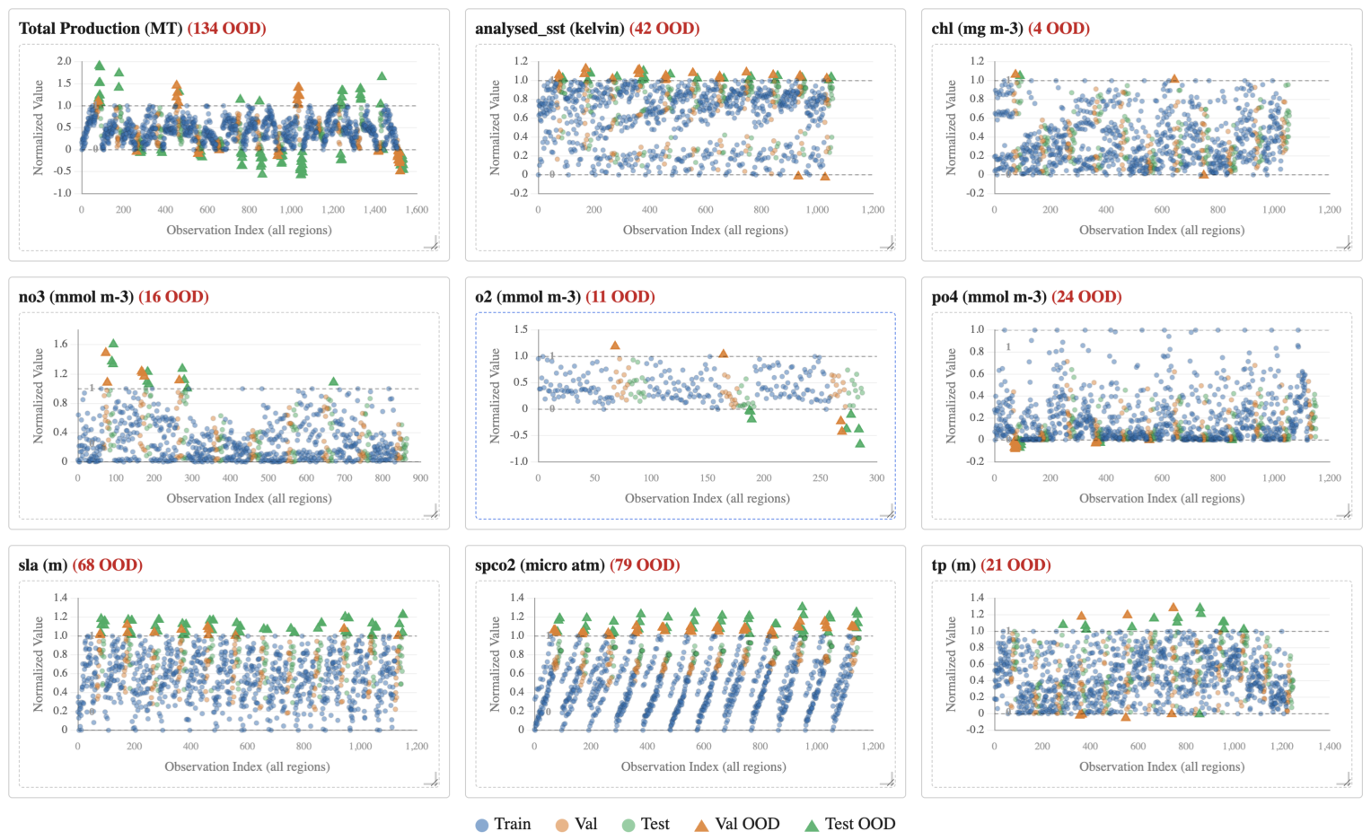
Figure A1 and Figure A2 quantify distribution shift between the training envelope and the held-out (validation + test) period, with any min–max-normalized value falling outside flagged as out of distribution (OOD).
The result is that the response variable itself was the most frequently OOD: total production was outside the training range in 28.9% of held-out cells (134/464) in both sectors, a direct consequence of the sustained post-2010 decline pushing recent production below historical minima. Among predictors, OOD rates spanned more than an order of magnitude and were concentrated in the monotonically trending climate variables—pCO2 (26.8% commercial, 22.7% marine municipal), sea level anomaly (17.0%, 19.5%), and SST (13.8%, 13.2%)—whereas chlorophyll-a, fluctuating around a quasi-stationary mean, was essentially never OOD (0.0% and 1.3%). The nutrient and freshwater predictors diverged by sector, with phosphate rising (2.0% → 6.9%) and rainfall falling (7.2% → 5.6%) from commercial to marine municipal, consistent with the marine municipal sector’s greater exposure to coastal nutrient regime shifts and the commercial sector’s exposure to rainfall-driven offshore variability.
Figure A1.
Out-of-distribution (OOD) analysis (commercial fisheries).
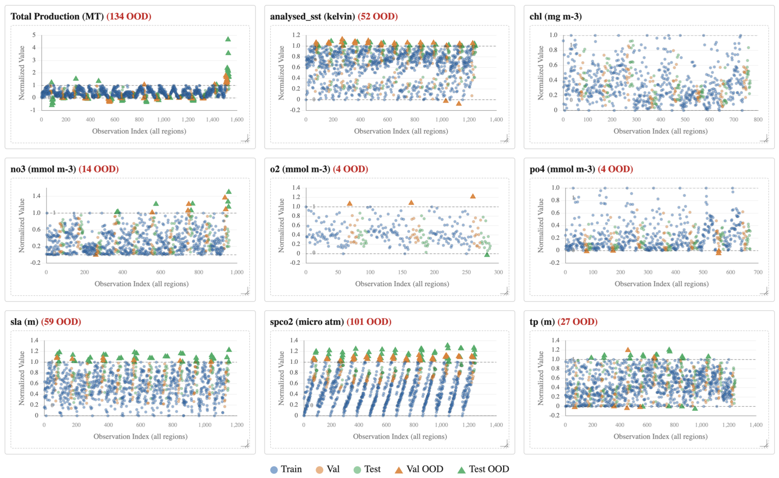
Figure A2.
Out-of-distribution (OOD) analysis (marine municipal fisheries).
Appendix B. Optuna Hyperparameter Tuning
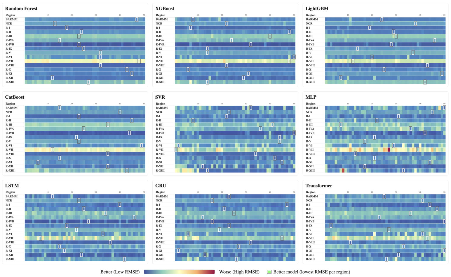
Figure A3 and Figure A4 report validation RMSE across all 16 regions × 50 Optuna trials for each of the nine candidate models. Tuning yielded substantial gains: relative to each model’s first trial, the selected best configuration reduced validation RMSE by a median of 33.4% (commercial) and 37.0% (marine municipal), reaching up to 90.0% and 81.2% in individual regions. In the commercial sector the winners were split across neural (8/16), tree-based (5/16), and classical (SVR, 3/16) families, whereas the marine municipal sector was overwhelmingly neural (12/16; MLP 5, LSTM 4, Transformer 3), suggesting its production series carry stronger nonlinear temporal structure. Held-out skill was heterogeneous: test ranged from to (commercial) and to (marine municipal), with near-zero medians ( and ) and median MAPE of 25.0% and 21.1%, respectively.
Figure A3.
Optuna hyperparameter tuning (commercial fisheries).
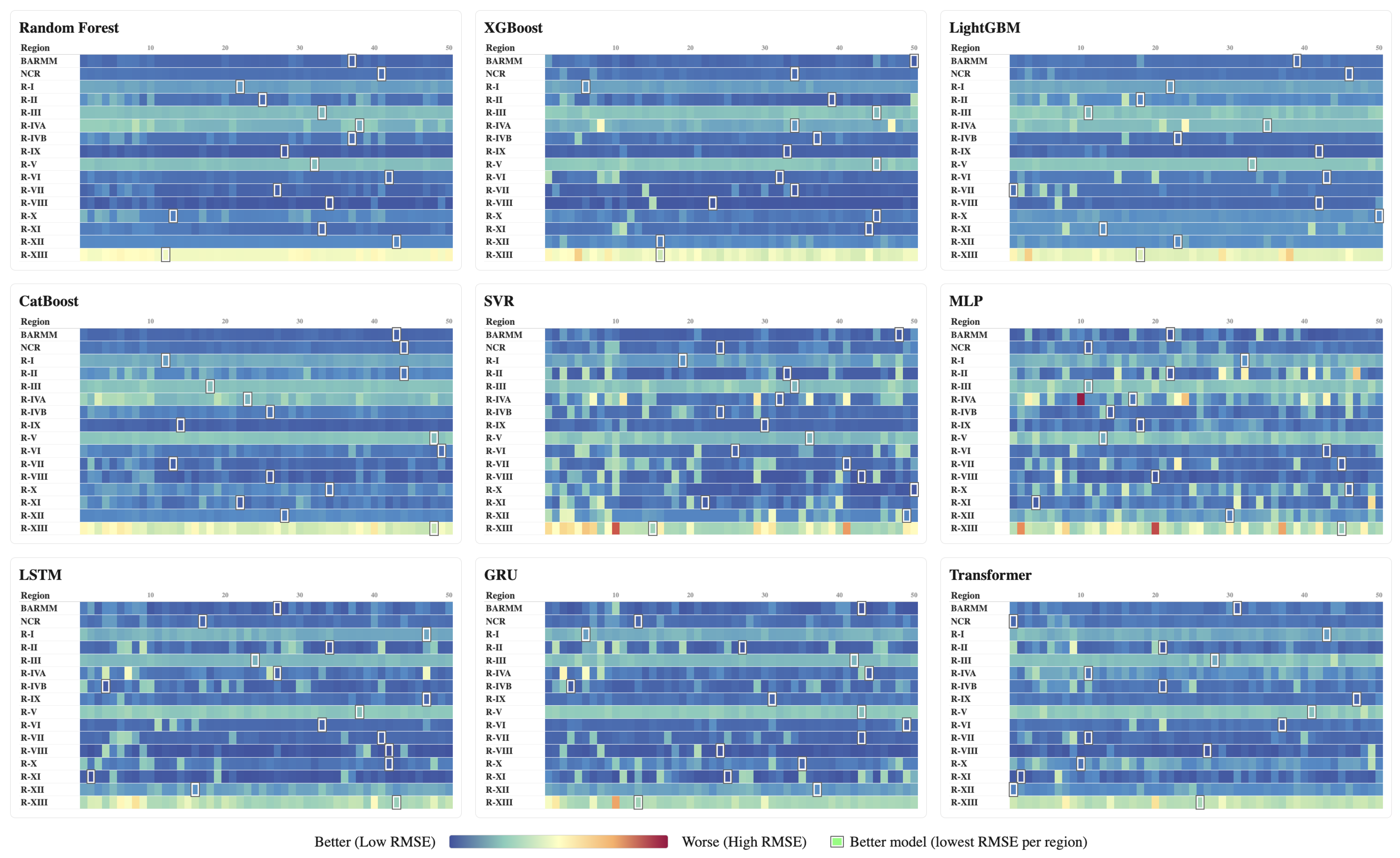
Figure A4.
Optuna hyperparameter tuning (marine municipal fisheries).
Appendix C. Actual vs. Predicted Time Series
Figure A5 and Figure A6 overlay actual (solid) and predicted (dashed) production for each region’s selected best model across the held-out validation (V) and test (T) periods. Only 4 of 16 commercial regions and a single marine municipal region achieved a test , though a majority returned positive test skill (8/16 and 10/16, respectively). A few regions were captured closely commercial Region IX (MLP, ), NCR (SVR, 0.81), and Region II (LSTM, 0.75), and marine municipal Region II (MLP, 0.92), where the predicted curve reproduced both the level and the direction of interannual change, whereas elsewhere the fitted series flattened toward the regional mean and missed sharp turning points, producing negative test (as low as in commercial Region XI and in marine municipal Region VII).
Figure A5.
Actual vs. predicted time series for each region (commercial fisheries).
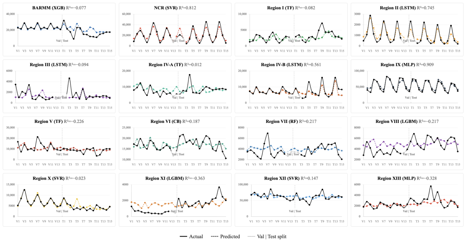
Figure A6.
Actual vs. predicted time series for each region (marine municipal fisheries).
Appendix D. SHAP Waterfall Plot
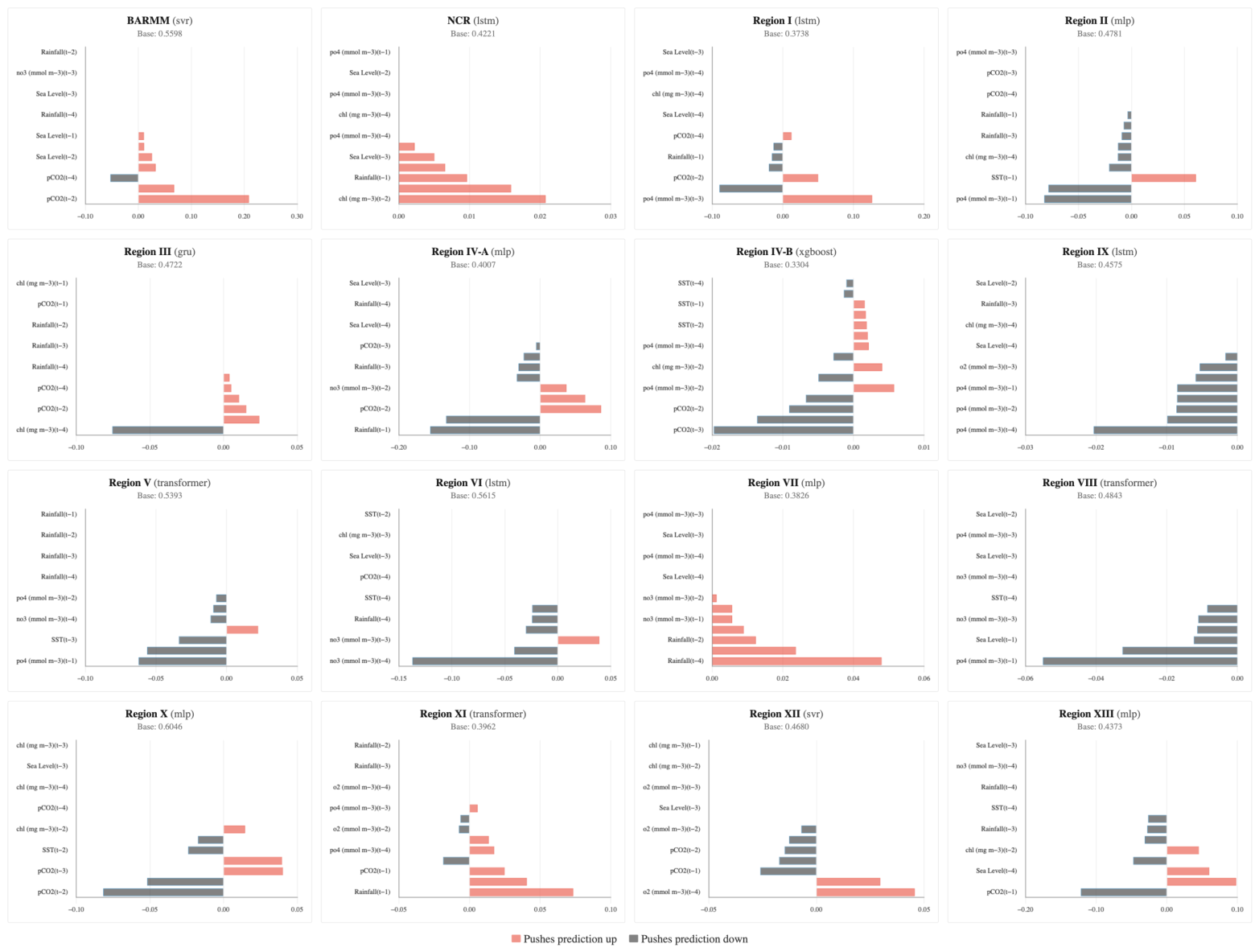
Figure A7 and Figure A8 show SHAP waterfall plots for representative held-out predictions from the Commercial and Marine Municipal sectors, respectively, tracing the progression from the base value (0.44 and 0.46, respectively) to the final predicted value via each feature’s signed SHAP contribution. Red bars increase the prediction; dark bars decrease it. The clearest pattern is that predictions are anchored by autoregressive terms: a lagged production feature is the single largest contributor in 12 of 16 commercial regions and 11 of 16 marine municipal regions, showing that recent past production, not environmental factors, drives the local signal. Each waterfall has approximately 11–14 active features, with the remainder excluded by per-region feature selection. Environmental predictors act as secondary modifiers, with rainfall the most common leading environmental factor (top driver in 3 commercial and 2 marine municipal regions). Contributions skew negative overall: most active features push predictions below the base value ( negative in both sectors), and the net effect is negative in 12 of 16 commercial and 9 of 16 marine municipal regions.
Figure A7.
SHAP waterfall plot (commercial fisheries).
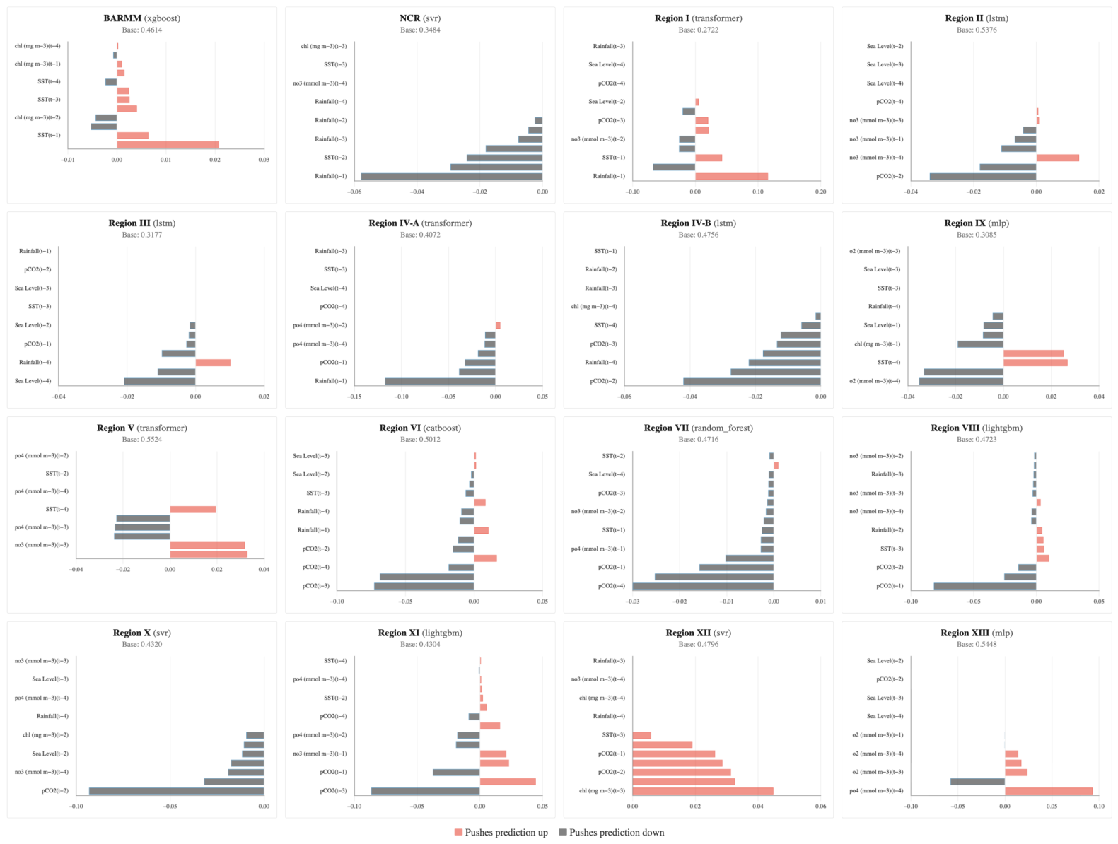
Figure A8.
SHAP waterfall plot (marine municipal fisheries).
Appendix E. SHAP Dependence
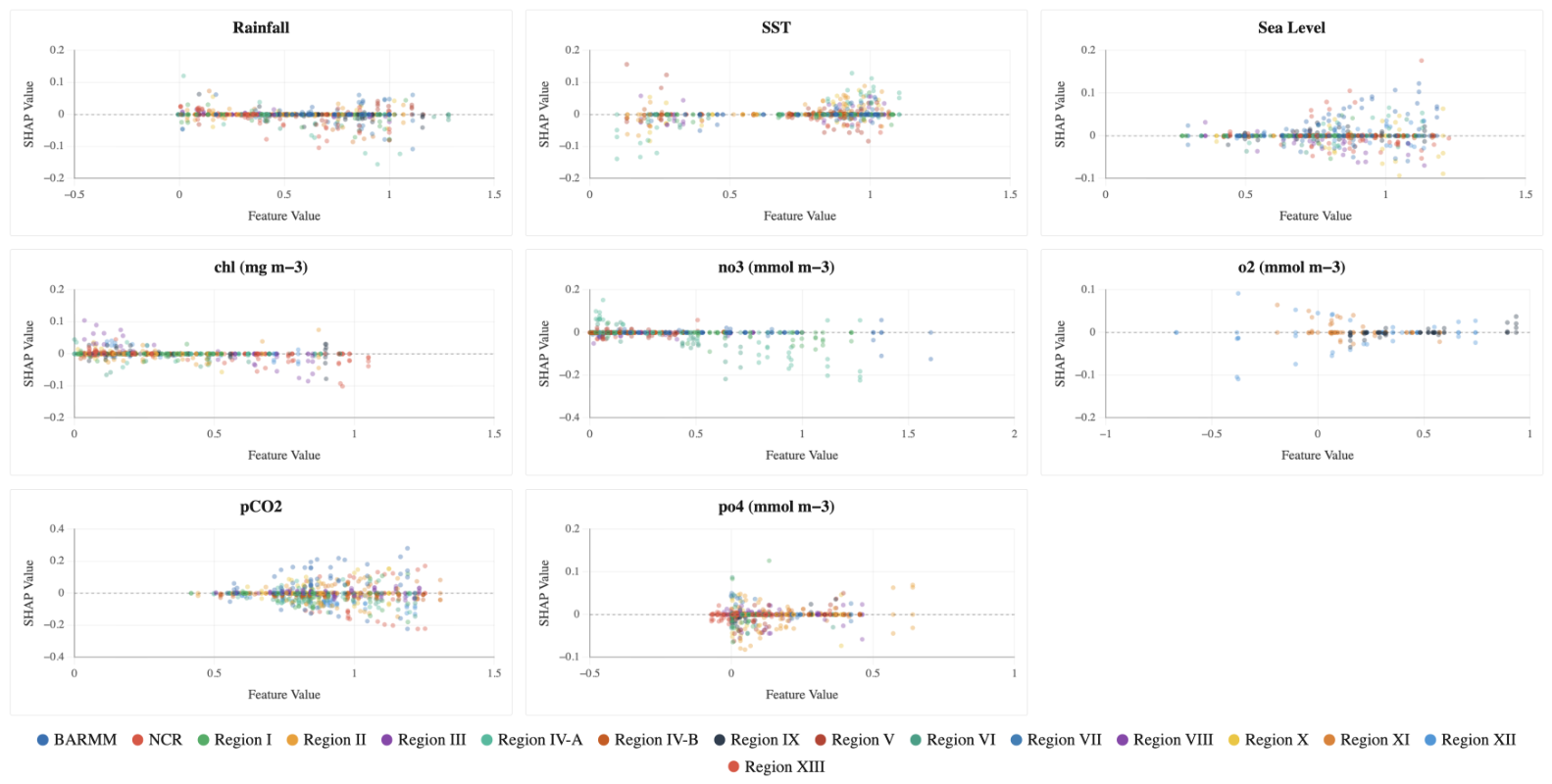
Figure A9 and Figure A10 plot the normalized values of each environmental feature against their corresponding SHAP contributions. Each point represents an individual observation from the test dataset () and is colored according to its region. The dashed horizontal line at distinguishes positive SHAP values, which increase the predicted fisheries production, from negative SHAP values, which decrease the prediction. The dominant pattern is that most feature–SHAP relationships are weak and, crucially, region-specific: for nearly every predictor the per-region slope changes sign across the color series rather than tracing a single shared curve, so the pooled trend is shallow ( for most features in both sectors). This visual divergence reinforces the heterogeneity seen in the forecasting results—environmental drivers act differently region by region rather than through one universal mechanism.
Figure A9.
SHAP dependence (commercial fisheries).
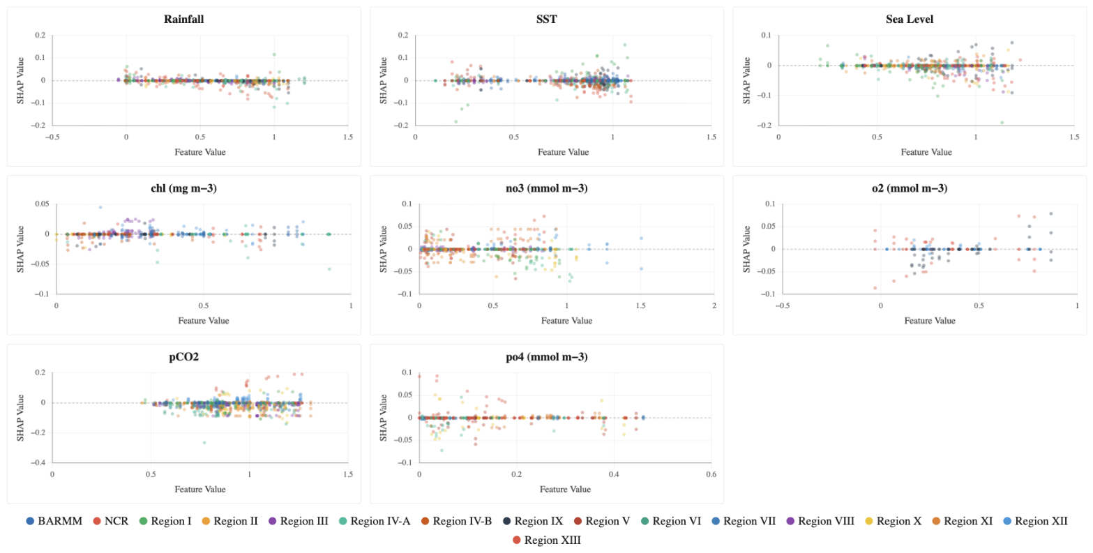
Figure A10.
SHAP dependence (marine municipal fisheries).
References
- Food and Agriculture Organization of the United Nations. The State of World Fisheries and Aquaculture 2024 — Blue Transformation in Action; FAO: Rome, Italy, 2024. [Google Scholar] [CrossRef] [Scilit]
- Béné, C.; Arthur, R.; Norbury, H.; Allison, E.H.; Beveridge, M.; Bush, S.; Campling, L.; Leschen, W.; Little, D.; Squires, D.; et al. Contribution of Fisheries and Aquaculture to Food Security and Poverty Reduction: Assessing the Current Evidence. World Dev. 2016, 79, 177–196. [Google Scholar] [CrossRef] [Scilit]
- Philippine Statistics Authority. Fisheries Situation Report, January to March 2026; Reference Number 2026-SSO-062; PSA: Quezon City, Philippines, 2026. Available online: https://psa.gov.ph/statistics/fisheries-situationer (accessed on 12 October 2025).
- Bureau of Fisheries and Aquatic Resources. Philippine Fisheries Profile 2022; Department of Agriculture: Quezon City, Philippines, 2024. Available online: https://www.bfar.da.gov.ph/ (accessed on 15 October 2025).
- Sustainable Fisheries Partnership. Better Seafood Philippines, 2022. Available online: https://sustainablefish.org/resilient-communities/better-seafood-philippines/ (accessed on 19 May 2026).
- Beaugrand, G.; Balembois, A.; Kléparski, L.; Kirby, R.R. Addressing the dichotomy of fishing and climate in fishery management with the FishClim model. Commun. Biol. 2022, 5, 1146. [Google Scholar] [CrossRef] [Scilit] [PubMed]
- Free, C.M.; Thorson, J.T.; Pinsky, M.L.; Oken, K.L.; Wiedenmann, J.; Jensen, O.P. Impacts of historical warming on marine fisheries production. Science 2019, 363, 979–983. [Google Scholar] [CrossRef] [Scilit] [PubMed]
- Sumaila, U.R.; de Fontaubert, C.; Palomares, M.L.D. Editorial: How overfishing handicaps resilience of marine resources under climate change. Front. Mar. Sci. 2023, 10, 1250449. [Google Scholar] [CrossRef] [Scilit]
- Cheng, L.; Abraham, J.; Trenberth, K.E.; Fasullo, J.; Boyer, T.; Mann, M.E.; Zhu, J.; Wang, F.; Locarnini, R.; Li, Y.; et al. Another record: Ocean warming continues through 2021 despite La Niña conditions. Adv. Atmos. Sci. 2022, 39, 373–385. [Google Scholar] [CrossRef] [Scilit] [PubMed]
- Doney, S.C.; Busch, D.S.; Cooley, S.R.; Kroeker, K.J. The impacts of ocean acidification on marine ecosystems and reliant human communities. Annu. Rev. Environ. Resour. 2020, 45, 83–112. [Google Scholar] [CrossRef] [Scilit]
- Pörtner, H.-O.; Roberts, D.C.; Tignor, M.; Poloczanska, E.S.; Mintenbeck, K.; Alegría, A.; Craig, M.; Langsdorf, S.; Löschke, S.; Möller, V.; et al. (Eds.) Climate Change 2022: Impacts, Adaptation and Vulnerability. Contribution of Working Group II to the Sixth Assessment Report of the Intergovernmental Panel on Climate Change; Cambridge University Press: Cambridge, UK, 2022. [Google Scholar] [CrossRef] [Scilit]
- Stock, C.A.; John, J.G.; Rykaczewski, R.R.; Asch, R.G.; Cheung, W.W.L.; Dunne, J.P.; Friedland, K.D.; Lam, V.W.Y.; Sarmiento, J.L.; Watson, R.A. Reconciling fisheries catch and ocean productivity. Proc. Natl. Acad. Sci. USA 2017, 114, E1441–E1449. [Google Scholar] [CrossRef] [Scilit] [PubMed]
- Tittensor, D.P.; Novaglio, C.; Harrison, C.S.; Heneghan, R.F.; Barrier, N.; Bianchi, D.; Bopp, L.; Bryndum-Buchholz, A.; Britten, G.L.; Bulman, C.M.; et al. Next-generation ensemble projections reveal higher climate risks for marine ecosystems. Nat. Clim. Change 2021, 11, 973–981. [Google Scholar] [CrossRef] [Scilit] [PubMed]
- Angelini, R.; Lima, M.A.L.; Lira, A.S.; Lucena-Frédou, F.; Frédou, T.; Bertrand, A.; Giarrizzo, T.; Steenbeek, J.; Coll, M.; Keppeler, F.W. The projected impacts of climate change and fishing pressure on a tropical marine food web. Mar. Environ. Res. 2025, 204, 106909. [Google Scholar] [CrossRef] [Scilit] [PubMed]
- Asch, R.G.; Thompson, A.R.; Auth, T.D.; Watson, W.; Brodeur, R.D.; Daly, E.A.; Suca, J.J. Continuing long-term shifts in larval fish phenology in the Southern California Current Ecosystem are matched by rapid advances in the North. Glob. Change Biol. 2025, 31, e70141. [Google Scholar] [CrossRef] [Scilit] [PubMed]
- Pinsky, M.L.; Selden, R.L.; Kitchel, Z.J. Climate-driven shifts in marine species ranges: Scaling from organisms to communities. Annu. Rev. Mar. Sci. 2020, 12, 153–179. [Google Scholar] [CrossRef] [Scilit] [PubMed]
- Bograd, S.J.; Anderson, L.C.; Canonico, G.; Chiba, S.; Di Lorenzo, E.; Enterline, C.; Gorecki, E.; Griffis, R.; Kleisner, K.M.; Lachance, H.; et al. Advancing the climate-biodiversity-fisheries nexus in the UN Decade of Ocean Science for Sustainable Development. ICES J. Mar. Sci. 2024, 81, 1705–1711. [Google Scholar] [CrossRef] [Scilit]
- Payne, M.R.; Danabasoglu, G.; Keenlyside, N.; Matei, D.; Miesner, A.K.; Yang, S.; Yeager, S.G. Skilful decadal-scale prediction of fish habitat and distribution shifts. Nat. Commun. 2022, 13, 2660. [Google Scholar] [CrossRef] [Scilit] [PubMed]
- Talbot, E.; Jontila, J.-B.S.; Gonzales, B.J.; Dolorosa, R.G.; Jose, E.D.; Sajorne, R.; Sailley, S.; Kay, S.; Queirós, A.M. Incorporating climate-readiness into fisheries management strategies. Sci. Total Environ. 2024, 918, 170684. [Google Scholar] [CrossRef] [Scilit] [PubMed]
- Liu, J.-M.; Borazon, E.Q.; Muñoz, K.E. Critical problems associated with climate change: A systematic review and meta-analysis of Philippine fisheries research. Environ. Sci. Pollut. Res. 2021, 28, 49425–49433. [Google Scholar] [CrossRef] [Scilit] [PubMed]
- Rasdas, S.M.; Costales, J.A.; Fajardo, A.C.; Limbago, J.S. Abundance mapping of commercial fisheries production using K-Means and forecasting algorithm in Manila Bay, Philippines. In Proceedings of the 2023 IEEE International Conference on Cybernetics and Innovations (I2CT); IEEE: Piscataway, NJ, USA, 2023; pp. 1–5. [Google Scholar] [CrossRef] [Scilit]
- Yñiguez, A.T.; Ottong, Z.J. Predicting fish kills and toxic blooms in an intensive mariculture site in the Philippines using a machine learning model. Sci. Total Environ. 2020, 707, 136173. [Google Scholar] [CrossRef] [Scilit] [PubMed]
- Kontopoulou, V.I.; Panagopoulos, A.D.; Kakkos, I.; Matsopoulos, G.K. A review of ARIMA vs. machine learning approaches for time series forecasting in data driven networks. Future Internet 2023, 15, 255. [Google Scholar] [CrossRef] [Scilit]
- Agmata, A.; Guðmundsson, S. Convolutional-LSTM approach for temporal catch hotspots (CATCH): An AI-driven model for spatiotemporal forecasting of fisheries catch probability densities. Biol. Methods Protoc. 2025, 10, bpaf045. [Google Scholar] [CrossRef] [Scilit] [PubMed]
- Vaswani, A.; Shazeer, N.; Parmar, N.; Uszkoreit, J.; Jones, L.; Gomez, A.N.; Kaiser, Ł.; Polosukhin, I. Attention is all you need. In Advances in Neural Information Processing Systems; Curran Associates: Red Hook, NY, USA, 2017; Volume 30, pp. 5998–6008. [Google Scholar]
- Lim, B.; Zohren, S. Time-series forecasting with deep learning: A survey. Philos. Trans. R. Soc. A 2021, 379, 20200209. [Google Scholar] [CrossRef] [Scilit] [PubMed]
- Reichstein, M.; Camps-Valls, G.; Stevens, B.; Jung, M.; Denzler, J.; Carvalhais, N.; Prabhat. Deep learning and process understanding for data-driven Earth system science. Nature 2019, 566, 195–204. [Google Scholar] [CrossRef] [Scilit] [PubMed]
- Hong, X.; Zhang, K.; Li, J.; Xu, Y.; Sun, M.; Xu, S.; Cai, Y.; Qiu, Y.; Chen, Z. Stock assessment of the commercial small pelagic fishes in the Beibu Gulf, the South China Sea, 2006–2020. Biology 2024, 13, 226. [Google Scholar] [CrossRef] [Scilit] [PubMed]
- Barredo Arrieta, A.; Díaz-Rodríguez, N.; Del Ser, J.; Bennetot, A.; Tabik, S.; Barbado, A.; García, S.; Gil-López, S.; Molina, D.; Benjamins, R.; et al. Explainable Artificial Intelligence (XAI): Concepts, taxonomies, opportunities and challenges toward responsible AI. Inf. Fusion 2020, 58, 82–115. [Google Scholar] [CrossRef] [Scilit]
- Saeed, W.; Omlin, C. Explainable AI (XAI): A systematic meta-survey of current challenges and future opportunities. Knowl.-Based Syst. 2023, 263, 110273. [Google Scholar] [CrossRef] [Scilit]
- Lundberg, S.M.; Erion, G.; Chen, H.; DeGrave, A.; Prutkin, J.M.; Nair, B.; Katz, R.; Himmelfarb, J.; Bansal, N.; Lee, S.-I. From local explanations to global understanding with explainable AI for trees. Nat. Mach. Intell. 2020, 2, 56–67. [Google Scholar] [CrossRef] [Scilit] [PubMed]
- Gilman, E.; Chaloupka, M.; Hall, M.; Hobday, A.J.; Kemp, H.; McMahon, C.R.; Murua, H.; Owens, D.; Suuronen, P.; Wallace, B. Evidence from interpretable machine learning to inform spatial management of Palau’s tuna fisheries. Ecosphere 2024, 15, e4751. [Google Scholar] [CrossRef] [Scilit]
- Lucas, T.C.D. A translucent box: Interpretable machine learning in ecology. Ecol. Monogr. 2020, 90, e01422. [Google Scholar] [CrossRef] [Scilit]
- Molnar, C.; Casalicchio, G.; Bischl, B. Interpretable machine learning—A brief history, state-of-the-art and challenges. In ECML PKDD 2020 Workshops; Communications in Computer and Information Science; Springer: Cham, Switzerland, 2020; Volume 1323, pp. 417–431. [Google Scholar] [CrossRef] [Scilit]
- Liu, L.; Wan, R.; Wu, F.; Wang, Y.; Zhu, Y.; Zhou, C. An integrative machine learning approach to understanding South Pacific Ocean albacore tuna habitat features. ICES J. Mar. Sci. 2025, 82, fsaf003. [Google Scholar] [CrossRef] [Scilit]
- Yang, L.; Zhou, W.; Zhang, C.; Tang, F. A comparative machine learning study identifies Light Gradient Boosting Machine (LightGBM) as the optimal model for unveiling the environmental drivers of yellowfin tuna (Thunnus albacares) Distrib. Using SHapley Addit. ExPlanations (SHAP) Analysis. Biology 2025, 14, 1567. [Google Scholar] [CrossRef] [Scilit] [PubMed]
- Rahman, L.F.; Marufuzzaman, M.; Alam, L.; Bari, M.A.; Sumaila, U.R.; Sidek, L.M. Developing an ensembled machine learning prediction model for marine fish and aquaculture production. Sustainability 2021, 13, 9124. [Google Scholar] [CrossRef] [Scilit]
- Ding, P.; Xu, H.; Zou, X.; Ding, S.; Bai, S. The relationship between the annual catch of bigeye tuna and climate factors and its prediction. Front. Mar. Sci. 2024, 11, 1344966. [Google Scholar] [CrossRef] [Scilit]
- Xie, M.; Liu, B.; Chen, X.; Yu, W.; Wang, J. Short- to medium-term forecasting of fishing ground distribution based on deep learning model. Can. J. Fish. Aquat. Sci. 2025, 82, 1–17. [Google Scholar] [CrossRef] [Scilit]
- Andriesse, E.; Fabinyi, M.; Foley, P.; Larsen, R.B.; Marschke, M. Small-scale fisheries, large-scale fisheries and fisheries governance in the Philippines. J. Environ. Policy Plan. 2024, 26, 159–172. [Google Scholar] [CrossRef] [Scilit]
- Lundberg, S.M.; Lee, S.-I. A unified approach to interpreting model predictions. In Advances in Neural Information Processing Systems; Curran Associates: Red Hook, NY, USA, 2017; Volume 30, pp. 4765–4774. [Google Scholar]
- Pedregosa, F.; Varoquaux, G.; Gramfort, A.; Michel, V.; Thirion, B.; Grisel, O.; Blondel, M.; Prettenhofer, P.; Weiss, R.; Dubourg, V.; et al. Scikit-learn: Machine learning in Python. J. Mach. Learn. Res. 2011, 12, 2825–2830. [Google Scholar]
- Chen, T.; Guestrin, C. XGBoost: A scalable tree boosting system. In Proceedings of the 22nd ACM SIGKDD International Conference on Knowledge Discovery and Data Mining; ACM: New York, NY, USA, 2016; pp. 785–794. [Google Scholar] [CrossRef] [Scilit]
- Ke, G.; Meng, Q.; Finley, T.; Wang, T.; Chen, W.; Ma, W.; Ye, Q.; Liu, T.-Y. LightGBM: A highly efficient gradient boosting decision tree. In Advances in Neural Information Processing Systems; Curran Associates: Red Hook, NY, USA, 2017; Volume 30, pp. 3146–3154. [Google Scholar]
- Prokhorenkova, L.; Gusev, G.; Vorobev, A.; Dorogush, A.V.; Gulin, A. CatBoost: Unbiased boosting with categorical features. In Advances in Neural Information Processing Systems; Curran Associates: Red Hook, NY, USA, 2018; Volume 31, pp. 6638–6648. [Google Scholar]
- Ansel, J.; Yang, E.; He, H.; Gimelshein, N.; Jain, A.; Voznesensky, M.; Bao, B.; Bell, P.; Berard, D.; Burovski, E.; et al. PyTorch 2: Faster machine learning through dynamic Python bytecode transformation and graph compilation. In Proceedings of the 29th ACM International Conference on Architectural Support for Programming Languages and Operating Systems (ASPLOS); Association for Computing Machinery: New York, NY, USA, 2024; pp. 929–947. [Google Scholar] [CrossRef] [Scilit]
- Paszke, A.; Gross, S.; Massa, F.; Lerer, A.; Bradbury, J.; Chanan, G.; Killeen, T.; Lin, Z.; Gimelshein, N.; Antiga, L.; et al. PyTorch: An imperative style, high-performance deep learning library. In Advances in Neural Information Processing Systems; Curran Associates: Red Hook, NY, USA, 2019; Volume 32, pp. 8024–8035. [Google Scholar]
- Akiba, T.; Sano, S.; Yanase, T.; Ohta, T.; Koyama, M. Optuna: A next-generation hyperparameter optimization framework. In Proceedings of the 25th ACM SIGKDD International Conference on Knowledge Discovery and Data Mining; ACM: New York, NY, USA, 2019; pp. 2623–2631. [Google Scholar] [CrossRef] [Scilit]
- Southeast Asian Fisheries Development Center. Fisheries Country Profile: Philippines 2025; SEAFDEC: Bangkok, Thailand, 2025; Available online: https://www.seafdec.org/fisheries-country-profile-philippines/ (accessed on 7 November 2025).
- Barboza, A.; Macusi, E.D.; Borazon, E.Q.; Santos, M.D.; Muallil, R.N.; Nallos, I.M. Small-scale fisheries (SSF) management and conservation schemes and their application in the Philippines. Mar. Policy 2024, 161, 106018. [Google Scholar] [CrossRef] [Scilit]
- National Mapping and Resource Information Authority. Official Philippine Shoreline Vector Dataset; Department of Environment and Natural Resources, Republic of the Philippines: Taguig City, Philippines, 2024. Available online: https://geoportal.gov.ph/ (accessed on 7 November 2025).
- Embury, O.; Merchant, C.J.; Good, S.A.; Rayner, N.A.; Atkinson, C.P.; Block, T.; Corlett, G.K.; Hollmann, R.; Killick, R.E.; Massey, L.; et al. Satellite-based time-series of sea-surface temperature since 1980 for climate applications. Sci. Data 2024, 11, 326. [Google Scholar] [CrossRef] [Scilit] [PubMed]
- Gregor, L.; Gruber, N. OceanSODA-ETHZ: A global gridded data set of the surface ocean carbonate system for seasonal to decadal studies of ocean acidification. Earth Syst. Sci. Data 2021, 13, 777–808. [Google Scholar] [CrossRef] [Scilit]
- Perruche, C.; Szczypta, C.; Paul, J.; Drévillon, M. Quality Information Document for Global Ocean Biogeochemistry Hindcast; Copernicus Marine Environment Monitoring Service: Toulouse, France, 2019; Available online: https://documentation.marine.copernicus.eu/QUID/CMEMS-GLO-QUID-001-029.pdf (accessed on 21 November 2025).
- von Schuckmann, K.; Minère, A.; Gues, F.; Cuesta-Valero, F.J.; Kirchengast, G.; Adusumilli, S.; Straneo, F.; Allan, R.; Barker, P.M.; Beltrami, H.; et al. Heat stored in the Earth system 1960–2020: Where does the energy go? Earth Syst. Sci. Data 2023, 15, 1675–1709. [Google Scholar] [CrossRef] [Scilit]
- Hersbach, H.; Bell, B.; Berrisford, P.; Hirahara, S.; Horányi, A.; Muñoz-Sabater, J.; Nicolas, J.; Peubey, C.; Radu, R.; Schepers, D.; et al. The ERA5 global reanalysis. Q. J. R. Meteorol. Soc. 2020, 146, 1999–2049. [Google Scholar] [CrossRef] [Scilit]
- Dallah, D.; Sulieman, H.; Alzaatreh, A.A.; Kamalov, F. Empirical evaluation of the relative range for detecting outliers. Entropy 2025, 27, 731. [Google Scholar] [CrossRef] [Scilit] [PubMed]
- Berendrecht, W.; van Vliet, M.; Griffioen, J. Combining statistical methods for detecting potential outliers in groundwater quality time series. Environ. Monit. Assess. 2023, 195, 85. [Google Scholar] [CrossRef] [Scilit] [PubMed]
- AlSalehy, A.S.; Bailey, M. Improving time series data quality: Identifying outliers and handling missing values in a multilocation gas and weather dataset. Smart Cities 2025, 8, 82. [Google Scholar] [CrossRef] [Scilit]
- Cai, W.; Santoso, A.; Collins, M.; Dewitte, B.; Karamperidou, C.; Kug, J.-S.; Lengaigne, M.; McPhaden, M.J.; Stuecker, M.F.; Taschetto, A.S.; et al. Changing El Niño–Southern Oscillation in a warming climate. Nat. Rev. Earth Environ. 2021, 2, 628–644. [Google Scholar] [CrossRef] [Scilit]
- Holbrook, N.J.; Scannell, H.A.; Sen Gupta, A.; Benthuysen, J.A.; Feng, M.; Oliver, E.C.J.; Alexander, L.V.; Burrows, M.T.; Donat, M.G.; Hobday, A.J.; et al. A global assessment of marine heatwaves and their drivers. Nat. Commun. 2019, 10, 2624. [Google Scholar] [CrossRef] [Scilit] [PubMed]
- Niedzielski, T.; Halicki, M. Improving linear interpolation of missing hydrological data by applying integrated autoregressive models. Water Resour. Manag. 2023, 37, 5707–5724. [Google Scholar] [CrossRef] [Scilit]
- Kapoor, S.; Narayanan, A. Leakage and the reproducibility crisis in machine-learning-based science. Patterns 2023, 4, 100804. [Google Scholar] [CrossRef] [Scilit] [PubMed]
- Lovakov, A.; Agadullina, E.R. Empirically derived guidelines for effect size interpretation in social psychology. Eur. J. Soc. Psychol. 2021, 51, 485–504. [Google Scholar] [CrossRef] [Scilit]
- Tong, R.; Yesson, C.; Yu, J.; Luo, Y.; Zhang, L. Key factors for species distribution modeling in benthic marine environments. Front. Mar. Sci. 2023, 10, 1222382. [Google Scholar] [CrossRef] [Scilit]
- Kalnins, A.; Praitis Hill, K. The VIF score. What is it good for? Absolutely nothing. Organ. Res. Methods 2025, 28, 58–75. [Google Scholar] [CrossRef] [Scilit]
- Zhang, H.-T.; Guo, W.-Y.; Wang, W.-T. The dimensionality reductions of environmental variables have a significant effect on the performance of species distribution models. Ecol. Evol. 2023, 13, e10747. [Google Scholar] [CrossRef] [Scilit] [PubMed]
- Collins, G.S.; Moons, K.G.M.; Dhiman, P.; Riley, R.D.; Beam, A.L.; Van Calster, B.; Ghassemi, M.; Liu, X.; Reitsma, J.B.; van Smeden, M.; et al. TRIPOD+AI statement: Updated guidance for reporting clinical prediction models that use regression or machine learning methods. BMJ 2024, 385, e078378. [Google Scholar] [CrossRef] [Scilit] [PubMed]
- García, S.; Luengo, J.; Herrera, F. Tutorial on practical tips of the most influential data preprocessing algorithms in data mining. Knowl.-Based Syst. 2016, 98, 1–29. [Google Scholar] [CrossRef] [Scilit]
- Bergmeir, C.; Hyndman, R.J.; Koo, B. A note on the validity of cross-validation for evaluating autoregressive time series prediction. Comput. Stat. Data Anal. 2018, 120, 70–83. [Google Scholar] [CrossRef] [Scilit]
- Bergstra, J.; Bardenet, R.; Bengio, Y.; Kégl, B. Algorithms for hyper-parameter optimization. In Advances in Neural Information Processing Systems; Curran Associates: Red Hook, NY, USA, 2011; Volume 24, pp. 2546–2554. [Google Scholar]
- Kingma, D.P.; Ba, J. Adam: A method for stochastic optimization. In Proceedings of the 3rd International Conference on Learning Representations, San Diego, CA, USA, 7–9 May 2015. [Google Scholar]
- Hodson, T.O. Root-mean-square error (RMSE) or mean absolute error (MAE): When to use them or not. Geosci. Model Dev. 2022, 15, 5481–5487. [Google Scholar] [CrossRef] [Scilit]
- Chicco, D.; Warrens, M.J.; Jurman, G. The coefficient of determination R-squared is more informative than SMAPE, MAE, MAPE, MSE and RMSE in regression analysis evaluation. PeerJ Comput. Sci. 2021, 7, e623. [Google Scholar] [CrossRef] [Scilit] [PubMed]
- Akshay, A.; Abedi, M.; Shekarchizadeh, N.; Burkhard, F.C.; Katoch, M.; Bigger-Allen, A.; Adam, R.M.; Monastyrskaya, K.; Hashemi Gheinani, A. MLcps: Machine learning cumulative performance score for classification problems. GigaScience 2023, 12, giad108. [Google Scholar] [CrossRef] [Scilit] [PubMed]
- Shapley, L.S. A value for n-person games. In Contributions to the Theory of Games, Volume II; Kuhn, H.W., Tucker, A.W., Eds.; Princeton University Press: Princeton, NJ, USA, 1953; pp. 307–317. [Google Scholar]
- Slack, D.; Hilgard, S.; Jia, E.; Singh, S.; Lakkaraju, H. Fooling LIME and SHAP: Adversarial attacks on post hoc explanation methods. In Proceedings of the AAAI/ACM Conference on AI, Ethics, and Society; ACM: New York, NY, USA, 2020; pp. 180–186. [Google Scholar] [CrossRef] [Scilit]
- Bonou, F.; Dossa, A.N.; Dahunsi, A.M.; Sohou, Z. Interannual and seasonal variability of CO2 parameters in the tropical Atlantic Ocean. J. Mar. Sci. Eng. 2024, 12, 2248. [Google Scholar] [CrossRef] [Scilit]
- Beliyana, E.; Ningsih, N.S.; Gunawan, S.R.; Tarya, A. Characteristics of marine heatwaves in the Indonesian waters during the PDO, ENSO, and IOD phases and their relationships to net surface heat flux. Atmosphere 2023, 14, 1035. [Google Scholar] [CrossRef] [Scilit]
- Santoso, A.; McPhaden, M.J.; Cai, W. The defining characteristics of ENSO extremes and the strong 2015/2016 El Niño. Rev. Geophys. 2017, 55, 1079–1129. [Google Scholar] [CrossRef] [Scilit]
- Hobday, A.J.; Alexander, L.V.; Perkins, S.E.; Smale, D.A.; Straub, S.C.; Oliver, E.C.J.; Benthuysen, J.A.; Burrows, M.T.; Donat, M.G.; Feng, M.; et al. A hierarchical approach to defining marine heatwaves. Prog. Oceanogr. 2016, 141, 227–238. [Google Scholar] [CrossRef] [Scilit]
- Chen, W.; Tong, Y.; Li, W.; Ding, Y.; Li, J.; Wang, W.; Shi, P. Interannual variations in the summer coastal upwelling in the northeastern South China Sea. Remote Sens. 2024, 16, 1282. [Google Scholar] [CrossRef] [Scilit]
- de Myttenaere, A.; Golden, B.; Le Grand, B.; Rossi, F. Mean Absolute Percentage Error for regression models. Neurocomputing 2016, 192, 38–48. [Google Scholar] [CrossRef] [Scilit]
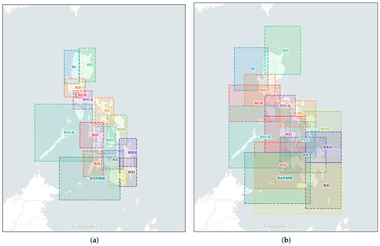
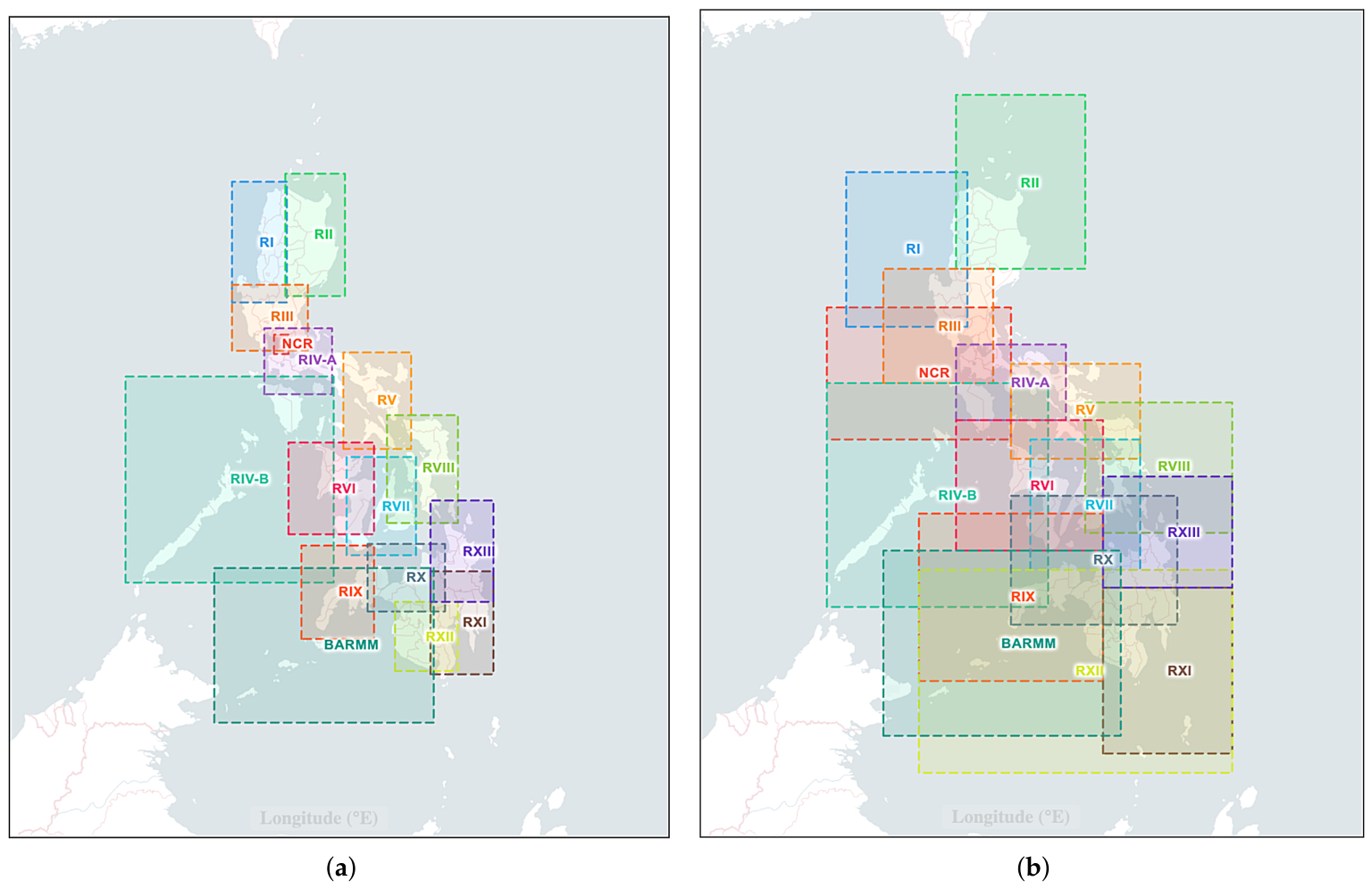
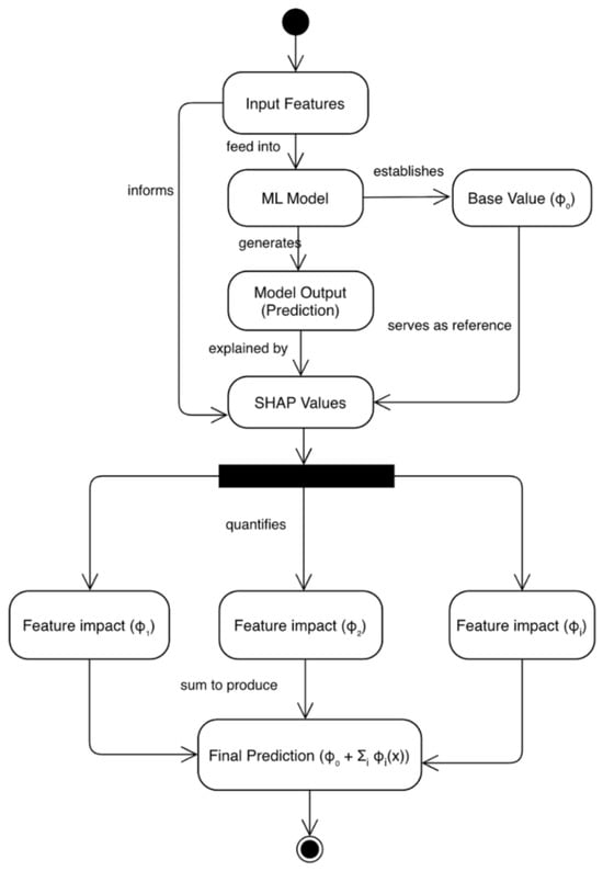
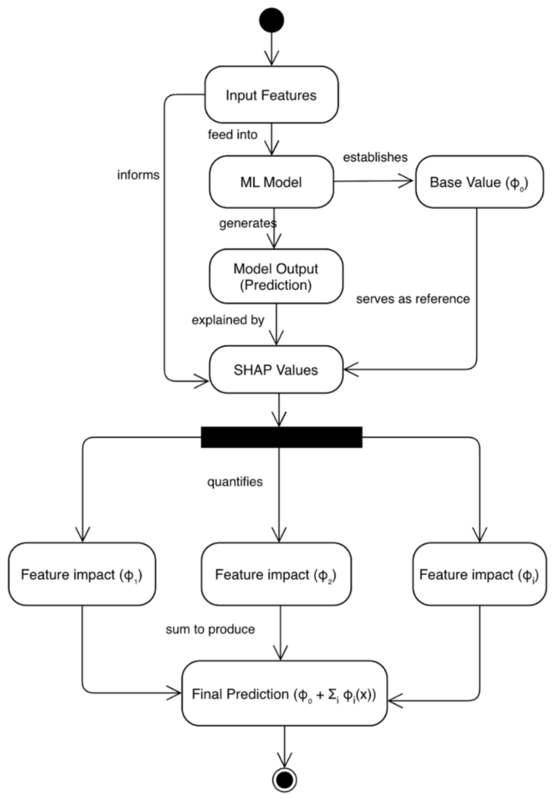
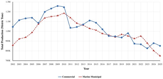
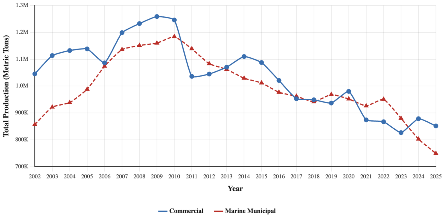
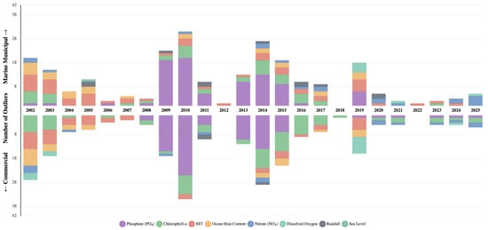
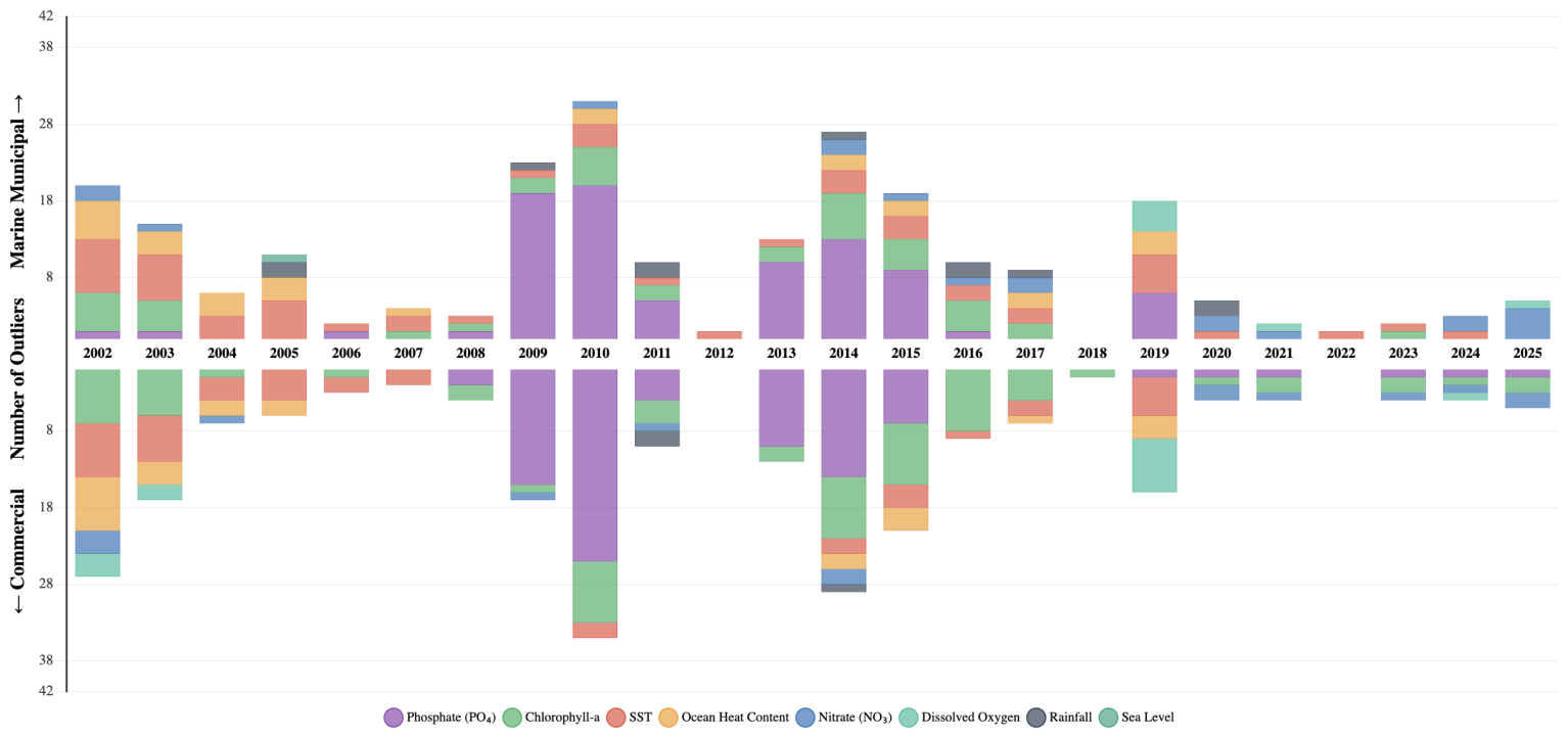
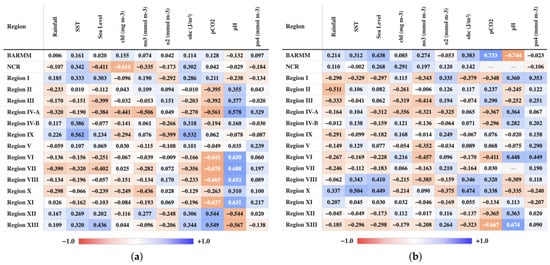
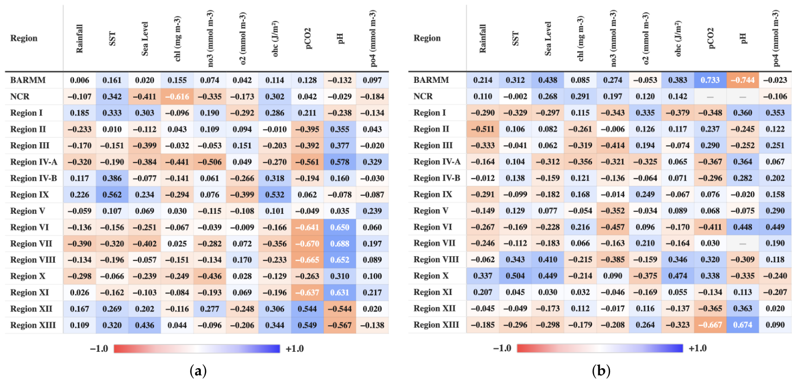
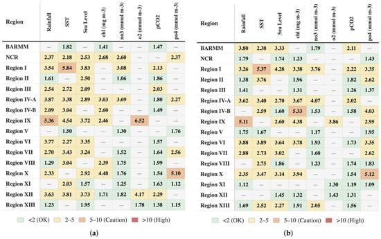
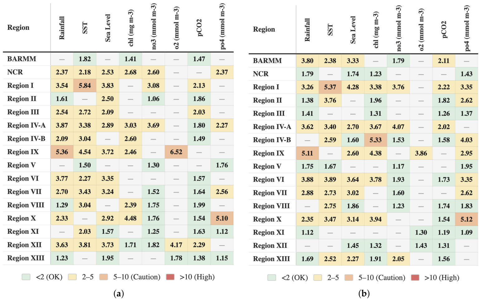
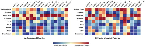
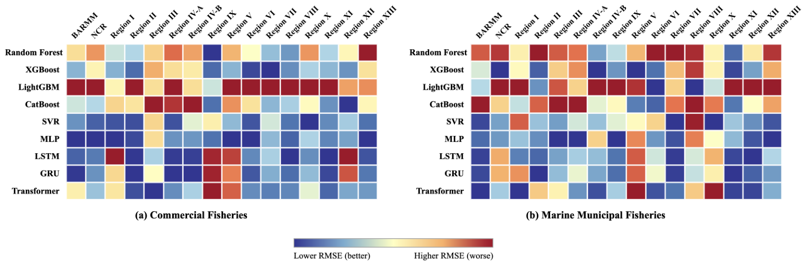
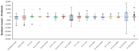
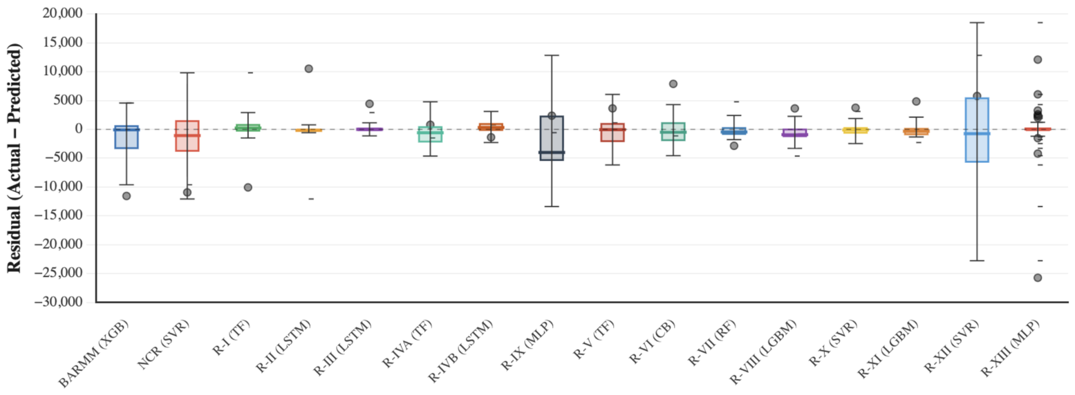
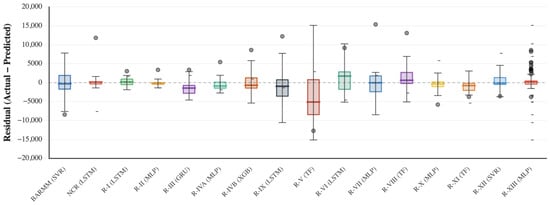
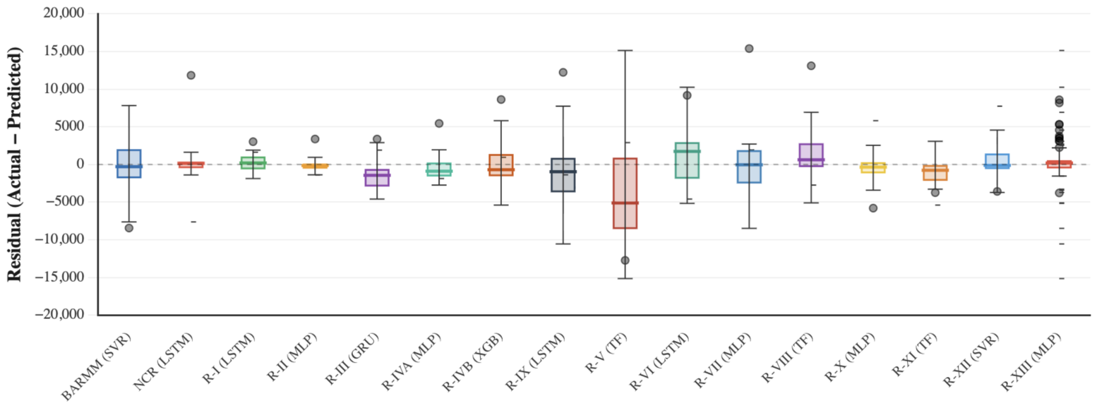
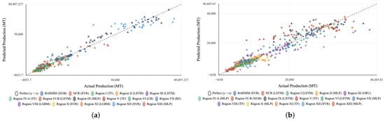
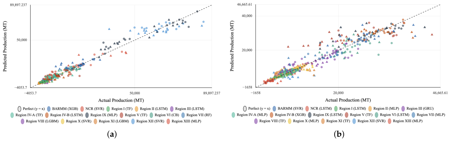
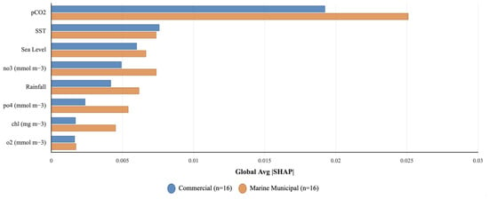
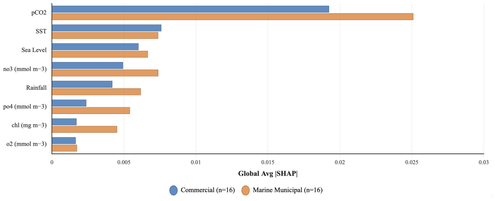
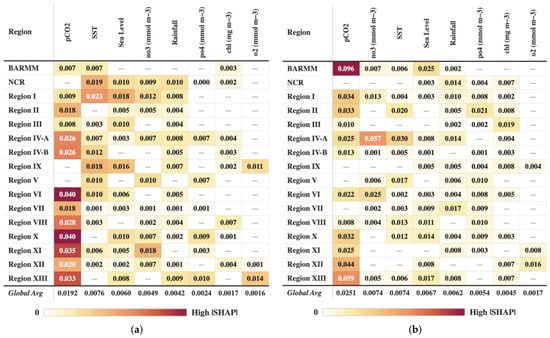
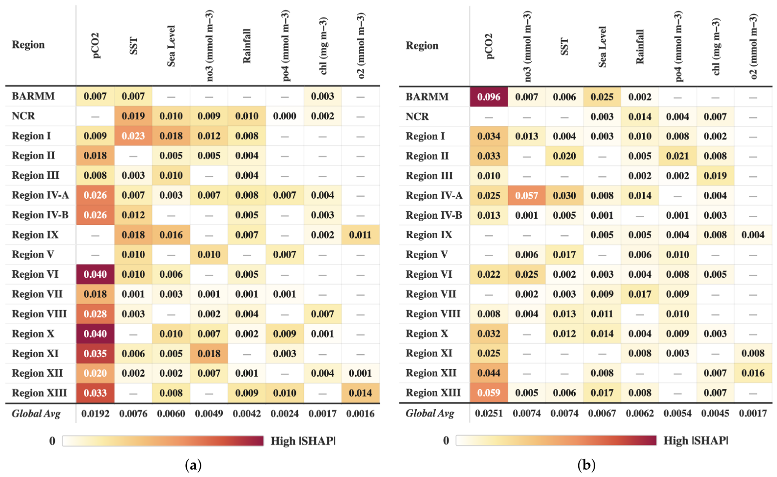

Disclaimer/Publisher’s Note: The statements, opinions and data contained in all publications are solely those of the individual author(s) and contributor(s) and not of MDPI and/or the editor(s). MDPI and/or the editor(s) disclaim responsibility for any injury to people or property resulting from any ideas, methods, instructions or products referred to in the content. |
© 2026 by the authors. Licensee MDPI, Basel, Switzerland. This article is an open access article distributed under the terms and conditions of the Creative Commons Attribution (CC BY) license.