Cancer Risk and Temporal Sequence Prediction of Prostate-Specific Antigen by Long Short-Term Memory Network

Abstract

Prostate-specific antigen (PSA) is a well-established marker for prostate cancer screening, but current ≥4 ng/mL cutoff suffers from low specificity. This study aims to demonstrate the use of a long short-term memory (LSTM) network for accurate prediction of prostate cancer risk and next sequential PSA value. Hong Kong-wide PSA test data over a 25-year period, including PSA values, time difference between PSA tests, and PSA velocity change, were retrieved for model training with variable PSA cutoffs and sequence length. A total of 1,158,915 PSA tests from 499,342 patients (including 18,629 patients with prostate cancer) were included. Models predicting the next PSA level performed well (accuracy 0.724–0.910, AUROC 0.751–0.892). For a ≥4 ng/mL cutoff, the best model was at sequence length of 4 (AUROC 0.864). Temporal prediction of PSA performance was lower (accuracy 0.739–0.811, AUROC 0.740–0.849). Prostate cancer prediction performed excellent (AUROC 0.888–0.973), the sensitivity (0.734), and specificity (0.962) were high even at the shortest sequence length and a ≥4 ng/mL cutoff (4). Utilizing PSA levels only without additional markers or clinical data, LSTM-based models accurately predicted the next PSA level with modest temporal predictions while significantly improving the specificity of prostate cancer risk prediction, demonstrating their clinical utility.

1. Introduction

Prostate cancer remains the second most frequently diagnosed malignancy among men globally, accounting for roughly 7.3% of all new male cancer mortalities [1]. With the common use of prostate-specific antigen (PSA), a key issue in prostate cancer screening pertains to how to identify true prostate cancer while avoiding over-investigation with invasive biopsies [2]. The currently commonly used binary approach of a cutoff at >4 μg/dL fails to account for benign confounding factors such as benign prostatic hyperplasia (BPH), prostatitis, and trauma, leading to significant diagnostic uncertainty where unnecessary biopsies are made unavoidable. PSA-based screening trials yielded a modest 20–31% reduction in prostate cancer mortality, with around 50% higher diagnosed incidence, much of which is overdiagnosis [3,4].

Today, we face an era with multiple advances in cancer diagnosis, including multiparametric Magnetic Resonance Imaging (mpMRI), genomic classifiers, and serum isoforms (such as the 4Kscore and Prostate Health Index). These tools have undeniably improved specificity, but they face significant barriers to implementation as primary population-level screening tools due to their limited availability, high costs, and requirement for specialized laboratory and radiological expertise [5]. While sequential PSA value, including PSA velocity, has seen success in prostate cancer disease monitoring, it has not been used for prostate cancer screening [6,7]. There remains a high interest in fully utilizing the stored information inside single and multiple PSA readings. Incorporating sequential PSA values is a potential approach for improving prostate cancer risk and future PSA-level prediction. The unresolved gap is that longitudinal PSA data are widely available, but there are no tools that use them well for risk stratification at the population level.

Machine learning, especially the long short-term memory (LSTM) networks, is a practical solution to this clinical problem. LSTM was designed to learn dependencies across time series data of varying lengths with non-uniform sampling and has outperformed cross-sectional models on prediction tasks based on electronic health record (EHR), including prediction of future cardiovascular health (CVH) category levels using previous CVH measurements and prediction of symptom trajectory in cancer cohort [8,9]. To our knowledge, no published work has applied LSTM to a territory-wide longitudinal PSA dataset to deliver a unified prostate cancer risk-stratification output for three prediction tasks, the next PSA level, the next PSA level with temporal prediction, and prostate cancer risk.

To address the gap, Hong Kong-wide PSA tests from 2000 to 2024 were retrieved in this study, comprising about 1.2 million PSA test results of 0.5 million patients, and used as input for LSTM training. The contributions of this study are (1) a population-scale longitudinal PSA dataset collected from laboratories under the Hospital Authority of Hong Kong using uniform standards, (2) a LSTM architecture covering three clinically aligned tasks rather than the risk-only prediction, and (3) a reproducible pipeline applicable to other PSA datasets. The aim of this study is to determine whether a single LSTM framework using only routinely collected PSA history can deliver clinically meaningful predictions across all three prediction tasks, thereby supporting more selective use of downstream investigations.

2. Materials and Methods

2.1. Data Collection

Data and results from PSA tests, including testing time, PSA value, and a unique reference number for each patient in Hong Kong, were retrieved through the Hong Kong Hospital Authority Clinical Data Analysis and Reporting System (CDARS) for the period 1 January 2000 to 31 December 2024. The ICD-9-CM codes of the patients were retrieved and reviewed for any diagnosis of “185: malignant neoplasm of prostate”. A case was defined as any diagnosis of prostate cancer during the included period, while a control was represented by the lack of a diagnosis. Records included those from the hospitals of all 7 public hospital clusters in Hong Kong (Hong Kong East Cluster, Hong Kong West Cluster, Kowloon Central Cluster, Kowloon East Cluster, Kowloon West Cluster, New Territories East Cluster, and New Territories West Cluster), incorporating 43 hospitals and institutions. Of these, records from 2 hospital clusters (Kowloon East Cluster and Kowloon West Cluster) comprising 8 hospitals were used as an external validation cohort. Patients were assigned to the external validation cohort only if all their records originated exclusively from the 8 hospitals.

PSA values and time points of each PSA test of each patient were matched. If multiple PSA values on the same day were present for a patient, only the highest PSA value for that day was included. Records with missing values were dropped. For patients with cancer occurrence, only PSA values measured more than 90 days before the diagnosis date were included in the study to avoid lead-time bias from PSA elevations associated with the impending diagnosis.

2.2. Target Prediction Variables

Prediction models for PSA were based on LSTM. Sequential PSA test results with corresponding time points and an indicator of prostate cancer occurrence for each patient were used as input to the models. The following prediction models were constructed based on the patients’ prior N consecutive PSA test values (all less than a predefined cutoff):

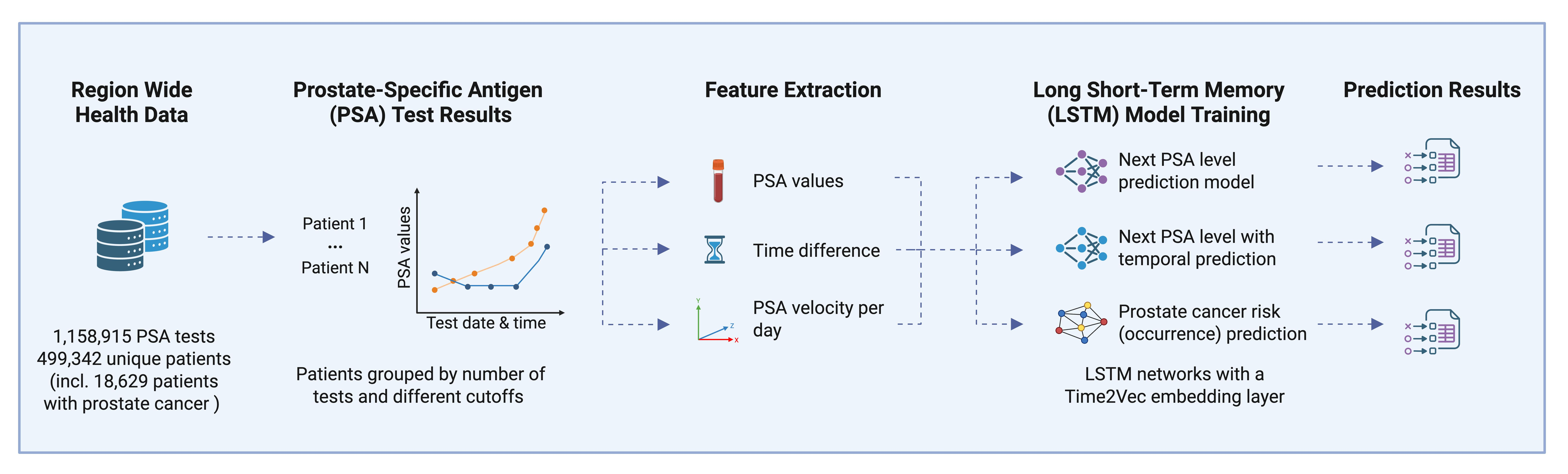
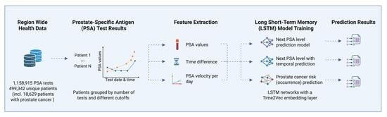
• Next-PSA-level prediction—whether the (N + 1) th PSA value exceeds a predefined cutoff.
• Next PSA level with temporal prediction—whether any PSA value exceeds a predefined cutoff in a certain future time interval (never, 0–12 months, 12 months+).
• Prostate cancer risk (occurrence) prediction—whether prostate cancer occurs.

2.3. Data Preparation

Prediction models were constructed for all combinations of different input sequence length (N) (4–9) and PSA cutoffs (≥4–≥9 ng/mL) to provide a systematic assessment of the model performance. For each combination of sequence length and PSA cutoffs, patients were selected if they had the first N PSA values all less than the predefined cutoff. Patients with fewer than N + 1 tests (N for model 3) were excluded.

The following features were extracted from each patient’s prior N consecutive PSA values at each time point:

• PSA values;
• $∆t$ (time difference between tests in days, starting with 0 for the initial test);
• PSA velocity change per day $(v_i=\left\{\begin{array}{c} 0, if i=0 or t_i-t_{i-1}=0\\ {\displaystyle \frac{{PSA}_i-{PSA}_{i-1}}{t_i-t_{i-1}}}, if i\ge 1 and t_i-t_{i-1}>0\end{array}\right.$).

These features were then used as input data to the models with a shape of (N, 3) for each patient.

Data were split at the patient level, producing an overall training/validation/test partition of eligible patients with a ratio of 60/20/20 (i.e., 80%/20% outer split, with the 80% further divided by a 4-fold cross-validation into 60% training and 20% validation). Standardization was performed using StandardScaler. Class imbalance was addressed by applying balanced class weight, computed per training fold. Data preparation was performed using the Pandas, NumPy, and scikit-learn libraries in Python (v3.12.2) [10,11,12].

2.4. Model Architecture and Training

A consistent architecture was employed in all models with different N and cutoffs using the TensorFlow framework and the Keras API [13,14]. For the input features, the $\mathrm{\Delta }t$ was fed into a Time2Vec ($t2\nu$) layer with K = 8, producing a learnable (K + 1)-dimensional embedding of a linear component concatenated with eight sinusoidal terms. The mathematical expression of $t2\nu$ for a given $\mathrm{\Delta }t$ was defined as follows:

$$t2\nu \left(\mathrm{\Delta }t\right)\left[i\right]= \left\{\begin{array}{c}{\omega }_i\mathrm{\Delta }t+{\phi }_i, if i=0.\\ \mathcal{F}\left({\omega }_i\mathrm{\Delta }t+{\phi }_i\right), if 1\le i\le k.\end{array}\right.$$

where the $t2\nu \left(\mathrm{\Delta }t\right)\left[i\right]$ is the ith element of $t2\nu \left(\mathrm{\Delta }t\right)$. $\mathcal{F}$ was a periodic activation function ($sin$), and both ${\omega }_i$ and ${\phi }_i$ were learnable parameters, allowing for the model to capture both periodic and non-periodic patterns of the input sequence [15]. The embedding was then concatenated with the two value channels (PSA values and PSA velocity) and normalized, then fed into a single LSTM layer with 64 units, a dropout rate of 0.35, and L2 regularization of 3 × 10⁻⁴, with returning sequence enabled. An attention-pooling layer then learned the normalized attention weights across time. A dropout layer with a rate of 0.35 was then applied before the final prediction layer. For binary models (models 1 and 3), the output layer used a single sigmoid unit, and for the multi-class model (model 2), three softmax units were used.

All models were trained for up to 50 epochs with a batch size of 64. The Adam optimizer with a learning rate of 3 × 10⁻⁴ and a gradient norm clipping of 1.0 was applied in the training. Early stopping with a patience of 10 and a learning rate reduction with a minimum learning rate of 1 × 10⁻⁵ and a patience of 5 were used. Platt calibration and F2-optimized thresholds were used in the binary models. For the multi-class model, multinomial Platt calibration and one-vs-rest F2-optimized thresholds were used, and the final class label was selected using the largest probability minus threshold margin.

2.5. Performance Assessment

Evaluation metrics of all models, including accuracy, sensitivity, specificity, Positive Predictive Value (PPV), Negative Predictive Value (NPV), the area under the receiver operating characteristic curve (AUROC), the area under the precision–recall curve (AUPRC), F1 score, and Brier score, were reported. The evaluation metrics for multi-class prediction models were macro-averaged across classes, with overall accuracy and Brier score reported as the multi-class classification metrics. To further access model performance, we generated a calibration plot and a clinical decision curve for the prostate cancer risk prediction model. Best-performing configurations (N and cutoff) were defined as the models yielding the best AUROC in each of the three prediction tasks. Bootstrapping (B = 1000) was used to estimate the 95% percentile confidence intervals (CIs). Partial Spearman rank correlations were assessed between each performance metric and two factors (N and cutoff), controlling separately for the other factor. Benjamini–Hochberg FDR (BH FDR) was applied to the permutation-based p-values for multiple testing correction. Data visualization was implemented using Matplotlib (v3.9.2) [16].

External validation was conducted using the model and configuration (N and cutoff) with the best AUROC in each prediction task and evaluated with the same set of metrics.

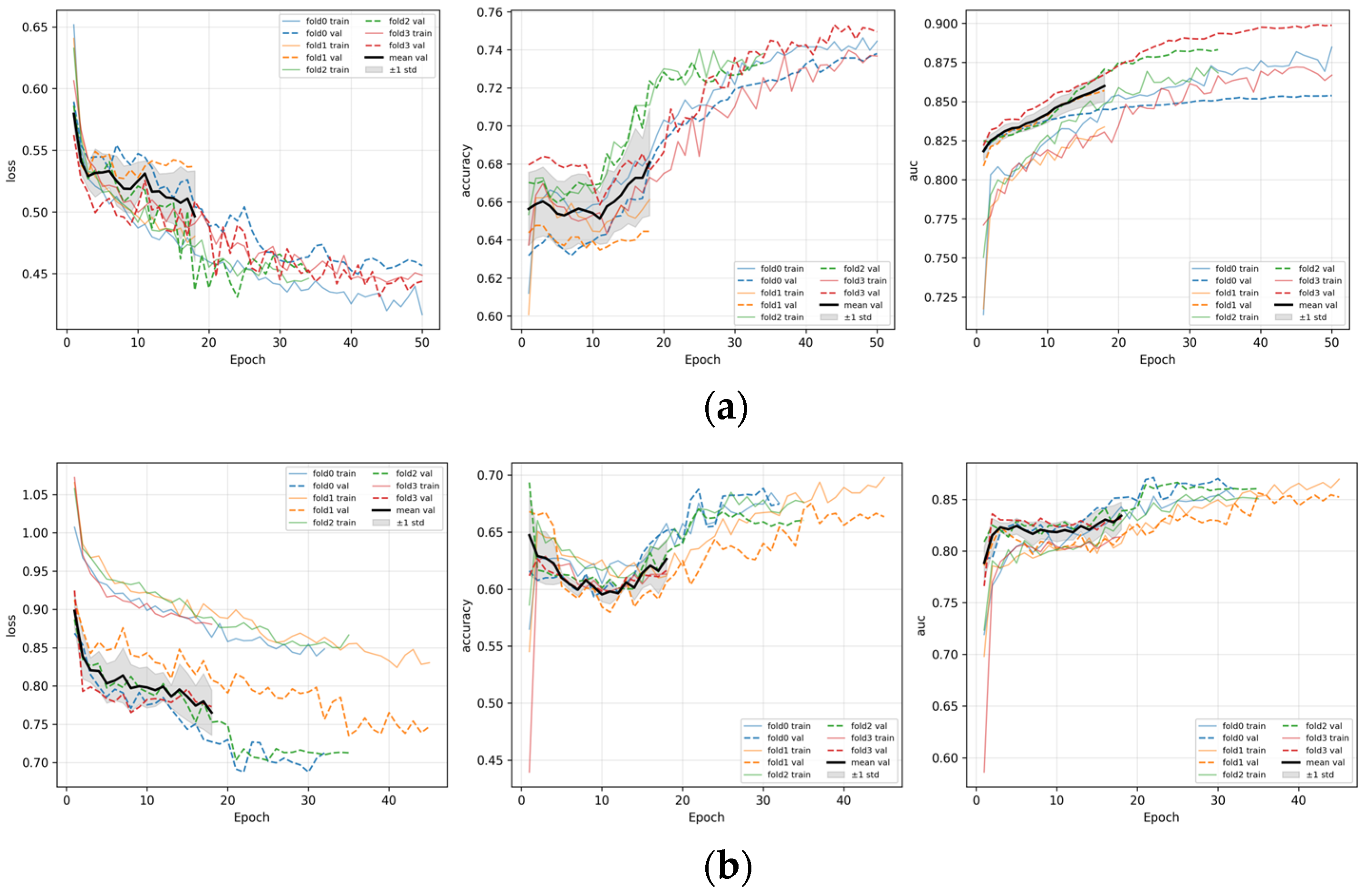
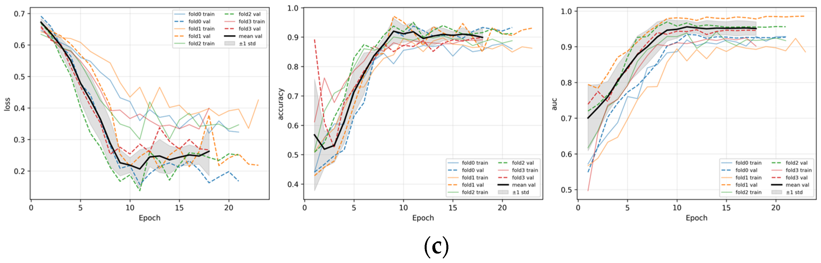
2.6. Model Transparency and Learning Dynamics Monitoring

In order to improve the model transparency, sample-level attention weights in PSA sequences were examined for the models achieving the best AUROC in each prediction task. To assess the individual contribution of each proposed architectural component (the Time2Vec layer, the attention-based pooling, and the PSA velocity features), we conducted an ablation study on three prediction tasks using the best-performing configurations. Learning dynamics, including model convergence, training stability, and potential overfitting, were assessed by tracking the training and validation loss, accuracy, and AUROC across the epochs and folds.

2.7. Baseline Recurrent Neural Network (RNN) and Logistic Regression

Simple baseline RNN and logistic regression models were constructed using the same settings and trained with the best performing configuration (N and cutoff) for each prediction model and evaluated using the same set of metrics.

3. Results

A total of 1,158,915 PSA tests from 499,342 unique patients (including 18,629 patients with prostate cancer) were included, with the number of eligible patients decreasing with increasing N and increasing with increasing PSA cutoffs. Of these, a total of 234,566 PSA tests from 112,467 patients were used as an independent external validation cohort.

3.1. Next-PSA-Level Prediction

Prediction models of different N and PSA cutoffs yielded overall accuracies ranging from 0.724 to 0.910 and AUROCs from 0.751 to 0.892. The best AUROC came from the model with N = 7 and cutoff = 6 (sample size = 1328, prevalence = 0.058), which achieved an overall accuracy of 0.852 and a Brier score of 0.046 (Figure 1a). Other metrics, including a sensitivity of 0.753, specificity of 0.859, NPV of 0.983, PPV of 0.247, F1 score of 0.372, and AUPRC of 0.359, were all recorded with 95% CIs in Appendix A 

Table A1. Metrics of next-PSA-level prediction—whether the (N + 1) th PSA value exceeds a predefined cutoff across input sequence lengths (N = 4–9) and PSA cutoffs (4–9 ng/mL).

N and Cutoff	Accuracy	Sensitivity	Specificity	Positive Predictive Value	Negative Predictive Value	F1 Score	AUROC	AUPRC	Brier Score	Prevalence
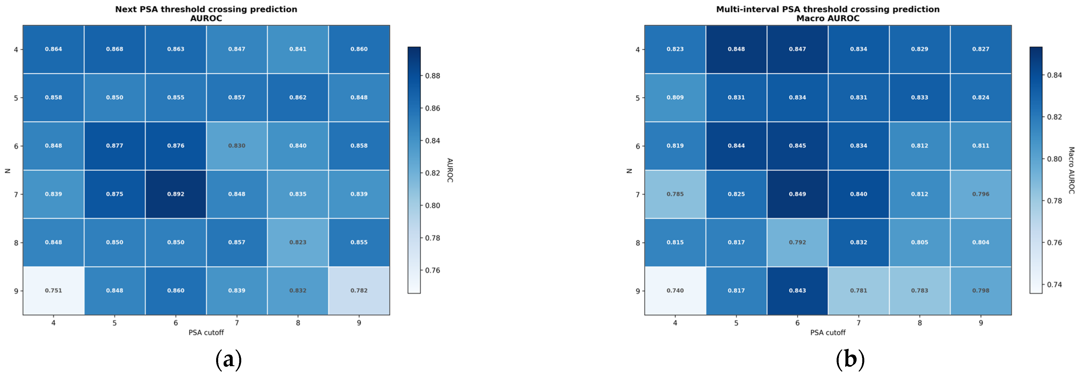
N = 4; Cutoff = 4	0.831 (0.819–0.846)	0.726 (0.660–0.797)	0.838 (0.825–0.852)	0.215 (0.182–0.251)	0.980 (0.975–0.986)	0.332 (0.290–0.378)	0.864 (0.836–0.891)	0.281 (0.230–0.357)	0.047 (0.041–0.053)	0.058
N = 4; Cutoff = 5	0.793 (0.779–0.805)	0.784 (0.732–0.838)	0.794 (0.780–0.806)	0.216 (0.188–0.242)	0.981 (0.976–0.986)	0.339 (0.303–0.373)	0.868 (0.847–0.885)	0.292 (0.247–0.351)	0.054 (0.048–0.059)	0.068
N = 4; Cutoff = 6	0.771 (0.759–0.783)	0.812 (0.768–0.854)	0.768 (0.755–0.781)	0.207 (0.185–0.229)	0.982 (0.977–0.986)	0.329 (0.300–0.360)	0.863 (0.846–0.880)	0.322 (0.276–0.372)	0.055 (0.051–0.060)	0.069
N = 4; Cutoff = 7	0.797 (0.787–0.808)	0.712 (0.665–0.757)	0.803 (0.792–0.814)	0.194 (0.173–0.217)	0.977 (0.972–0.981)	0.304 (0.277–0.335)	0.847 (0.829–0.865)	0.262 (0.223–0.315)	0.051 (0.047–0.057)	0.062
N = 4; Cutoff = 8	0.806 (0.796–0.816)	0.695 (0.643–0.746)	0.812 (0.802–0.822)	0.168 (0.147–0.190)	0.980 (0.976–0.984)	0.270 (0.239–0.301)	0.841 (0.820–0.861)	0.235 (0.197–0.285)	0.044 (0.039–0.048)	0.052
N = 4; Cutoff = 9	0.850 (0.841–0.859)	0.667 (0.609–0.722)	0.858 (0.849–0.867)	0.175 (0.152–0.198)	0.983 (0.979–0.986)	0.277 (0.246–0.308)	0.860 (0.840–0.878)	0.212 (0.176–0.255)	0.037 (0.033–0.041)	0.043
N = 5; Cutoff = 4	0.844 (0.826–0.859)	0.671 (0.569–0.775)	0.853 (0.835–0.869)	0.188 (0.144–0.231)	0.981 (0.974–0.987)	0.294 (0.234–0.350)	0.858 (0.821–0.892)	0.233 (0.170–0.320)	0.041 (0.034–0.049)	0.048
N = 5; Cutoff = 5	0.805 (0.788–0.821)	0.715 (0.641–0.785)	0.811 (0.794–0.828)	0.207 (0.175–0.243)	0.976 (0.969–0.983)	0.321 (0.278–0.368)	0.850 (0.819–0.878)	0.253 (0.207–0.320)	0.053 (0.046–0.060)	0.065
N = 5; Cutoff = 6	0.778 (0.762–0.793)	0.750 (0.685–0.805)	0.780 (0.764–0.796)	0.192 (0.164–0.219)	0.978 (0.971–0.984)	0.306 (0.267–0.343)	0.855 (0.830–0.875)	0.295 (0.241–0.364)	0.054 (0.047–0.060)	0.065
N = 5; Cutoff = 7	0.801 (0.787–0.814)	0.723 (0.660–0.785)	0.806 (0.792–0.820)	0.186 (0.159–0.212)	0.979 (0.974–0.985)	0.296 (0.259–0.331)	0.857 (0.834–0.878)	0.243 (0.201–0.300)	0.048 (0.043–0.054)	0.058
N = 5; Cutoff = 8	0.820 (0.809–0.832)	0.723 (0.662–0.781)	0.826 (0.813–0.837)	0.186 (0.158–0.213)	0.982 (0.977–0.986)	0.296 (0.257–0.332)	0.862 (0.839–0.882)	0.228 (0.192–0.282)	0.044 (0.039–0.049)	0.052
N = 5; Cutoff = 9	0.867 (0.857–0.877)	0.572 (0.498–0.643)	0.881 (0.871–0.891)	0.180 (0.149–0.214)	0.978 (0.973–0.983)	0.274 (0.231–0.318)	0.848 (0.824–0.872)	0.215 (0.170–0.276)	0.038 (0.033–0.043)	0.044
N = 6; Cutoff = 4	0.806 (0.784–0.831)	0.786 (0.659–0.907)	0.807 (0.784–0.831)	0.133 (0.094–0.177)	0.990 (0.983–0.996)	0.228 (0.167–0.291)	0.848 (0.796–0.893)	0.153 (0.099–0.251)	0.032 (0.024–0.042)	0.036
N = 6; Cutoff = 5	0.846 (0.829–0.864)	0.713 (0.614–0.808)	0.854 (0.836–0.871)	0.220 (0.171–0.271)	0.981 (0.973–0.988)	0.336 (0.270–0.401)	0.877 (0.843–0.905)	0.251 (0.187–0.347)	0.045 (0.036–0.053)	0.055
N = 6; Cutoff = 6	0.787 (0.768–0.804)	0.832 (0.760–0.899)	0.784 (0.764–0.801)	0.206 (0.170–0.242)	0.986 (0.980–0.992)	0.330 (0.280–0.377)	0.876 (0.850–0.901)	0.265 (0.211–0.347)	0.050 (0.044–0.058)	0.063
N = 6; Cutoff = 7	0.724 (0.706–0.742)	0.820 (0.759–0.882)	0.718 (0.700–0.737)	0.150 (0.126–0.176)	0.985 (0.979–0.991)	0.254 (0.216–0.291)	0.830 (0.802–0.854)	0.195 (0.153–0.253)	0.049 (0.043–0.056)	0.057
N = 6; Cutoff = 8	0.826 (0.812–0.840)	0.664 (0.584–0.743)	0.835 (0.821–0.848)	0.180 (0.146–0.212)	0.978 (0.972–0.984)	0.284 (0.237–0.327)	0.840 (0.806–0.870)	0.262 (0.206–0.338)	0.044 (0.038–0.050)	0.052
N = 6; Cutoff = 9	0.869 (0.856–0.881)	0.569 (0.484–0.651)	0.883 (0.871–0.895)	0.188 (0.154–0.224)	0.977 (0.972–0.983)	0.282 (0.235–0.330)	0.858 (0.833–0.882)	0.224 (0.173–0.297)	0.039 (0.033–0.044)	0.045
N = 7; Cutoff = 4	0.853 (0.829–0.878)	0.630 (0.435–0.818)	0.861 (0.837–0.884)	0.134 (0.078–0.197)	0.986 (0.976–0.994)	0.221 (0.135–0.310)	0.839 (0.768–0.901)	0.198 (0.098–0.362)	0.030 (0.020–0.041)	0.033
N = 7; Cutoff = 5	0.846 (0.823–0.868)	0.702 (0.561–0.829)	0.852 (0.830–0.873)	0.186 (0.129–0.250)	0.983 (0.974–0.991)	0.295 (0.212–0.377)	0.875 (0.834–0.911)	0.276 (0.171–0.414)	0.039 (0.030–0.049)	0.046
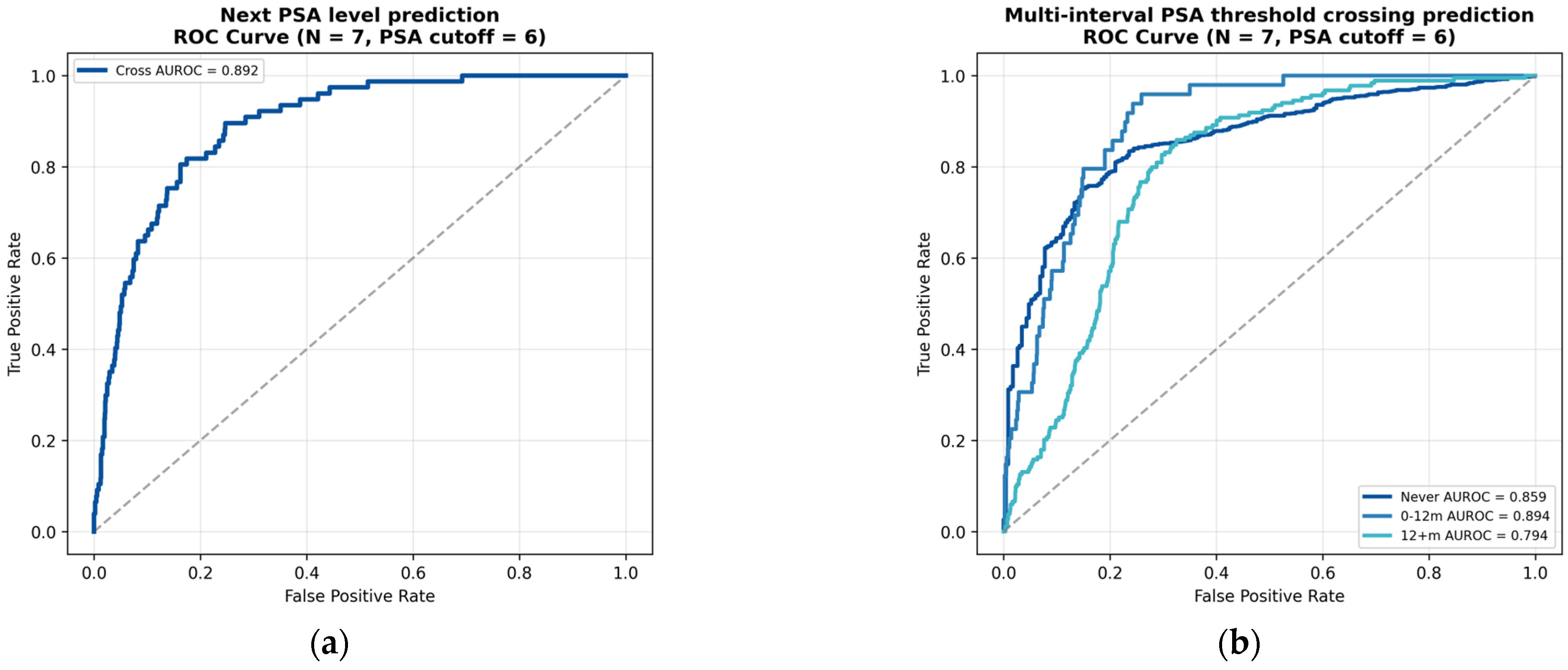
N = 7; Cutoff = 6	0.852 (0.833–0.871)	0.753 (0.659–0.847)	0.859 (0.838–0.878)	0.247 (0.189–0.306)	0.983 (0.975–0.990)	0.372 (0.299–0.443)	0.892 (0.859–0.923)	0.359 (0.264–0.474)	0.046 (0.037–0.056)	0.058
N = 7; Cutoff = 7	0.788 (0.769–0.808)	0.736 (0.637–0.819)	0.791 (0.771–0.811)	0.170 (0.134–0.208)	0.981 (0.973–0.988)	0.276 (0.223–0.327)	0.848 (0.816–0.879)	0.250 (0.175–0.340)	0.047 (0.039–0.055)	0.055
N = 7; Cutoff = 8	0.753 (0.734–0.772)	0.760 (0.680–0.843)	0.753 (0.733–0.773)	0.137 (0.109–0.168)	0.984 (0.977–0.990)	0.232 (0.190–0.277)	0.835 (0.803–0.867)	0.192 (0.143–0.267)	0.043 (0.036–0.051)	0.049
N = 7; Cutoff = 9	0.819 (0.804–0.834)	0.689 (0.600–0.776)	0.826 (0.810–0.840)	0.165 (0.131–0.200)	0.981 (0.976–0.987)	0.266 (0.217–0.315)	0.839 (0.806–0.873)	0.214 (0.155–0.289)	0.041 (0.035–0.048)	0.048
N = 8; Cutoff = 4	0.910 (0.887–0.931)	0.471 (0.235–0.714)	0.922 (0.901–0.942)	0.148 (0.062–0.255)	0.984 (0.972–0.993)	0.225 (0.100–0.356)	0.848 (0.768–0.916)	0.225 (0.088–0.436)	0.026 (0.016–0.038)	0.028
N = 8; Cutoff = 5	0.857 (0.832–0.883)	0.519 (0.320–0.714)	0.870 (0.846–0.895)	0.131 (0.070–0.198)	0.980 (0.968–0.991)	0.209 (0.117–0.304)	0.850 (0.773–0.907)	0.185 (0.093–0.315)	0.032 (0.022–0.043)	0.036
N = 8; Cutoff = 6	0.803 (0.778–0.828)	0.686 (0.555–0.809)	0.810 (0.784–0.836)	0.169 (0.119–0.221)	0.979 (0.968–0.988)	0.271 (0.197–0.344)	0.850 (0.810–0.885)	0.215 (0.142–0.323)	0.045 (0.035–0.056)	0.053
N = 8; Cutoff = 7	0.776 (0.752–0.798)	0.833 (0.729–0.921)	0.774 (0.748–0.796)	0.161 (0.123–0.204)	0.989 (0.981–0.995)	0.270 (0.213–0.328)	0.857 (0.808–0.896)	0.211 (0.151–0.309)	0.042 (0.034–0.052)	0.050
N = 8; Cutoff = 8	0.788 (0.766–0.807)	0.648 (0.533–0.754)	0.796 (0.773–0.815)	0.141 (0.104–0.179)	0.978 (0.968–0.986)	0.232 (0.175–0.286)	0.823 (0.780–0.866)	0.181 (0.129–0.264)	0.043 (0.035–0.052)	0.049
N = 8; Cutoff = 9	0.820 (0.801–0.838)	0.694 (0.584–0.800)	0.825 (0.807–0.843)	0.153 (0.116–0.194)	0.983 (0.977–0.990)	0.251 (0.195–0.308)	0.855 (0.818–0.890)	0.216 (0.150–0.304)	0.038 (0.031–0.045)	0.044
N = 9; Cutoff = 4	0.874 (0.844–0.905)	0.400 (0.111–0.715)	0.885 (0.856–0.914)	0.071 (0.017–0.146)	0.985 (0.973–0.995)	0.121 (0.030–0.229)	0.751 (0.556–0.902)	0.116 (0.032–0.367)	0.021 (0.009–0.032)	0.022
N = 9; Cutoff = 5	0.761 (0.723–0.797)	0.812 (0.600–1.000)	0.760 (0.721–0.796)	0.092 (0.046–0.140)	0.993 (0.983–1.000)	0.165 (0.087–0.241)	0.848 (0.770–0.920)	0.141 (0.065–0.300)	0.027 (0.015–0.038)	0.029
N = 9; Cutoff = 6	0.790 (0.760–0.820)	0.727 (0.571–0.871)	0.793 (0.762–0.823)	0.147 (0.097–0.200)	0.983 (0.972–0.993)	0.245 (0.168–0.322)	0.860 (0.803–0.905)	0.199 (0.129–0.320)	0.041 (0.029–0.053)	0.047
N = 9; Cutoff = 7	0.775 (0.747–0.803)	0.729 (0.595–0.855)	0.778 (0.750–0.805)	0.157 (0.113–0.205)	0.981 (0.968–0.990)	0.258 (0.194–0.325)	0.839 (0.791–0.880)	0.211 (0.138–0.326)	0.046 (0.036–0.058)	0.054
N = 9; Cutoff = 8	0.779 (0.755–0.806)	0.660 (0.534–0.781)	0.785 (0.761–0.811)	0.138 (0.097–0.184)	0.978 (0.968–0.987)	0.228 (0.168–0.294)	0.832 (0.779–0.876)	0.229 (0.149–0.345)	0.043 (0.033–0.054)	0.050
N = 9; Cutoff = 9	0.791 (0.768–0.812)	0.588 (0.455–0.718)	0.799 (0.776–0.821)	0.112 (0.075–0.149)	0.978 (0.969–0.987)	0.188 (0.128–0.242)	0.782 (0.727–0.833)	0.115 (0.076–0.177)	0.038 (0.029–0.047)	0.041

. At a PSA cutoff of 4, the model with a N = 4 achieved the best AUROC of 0.864, with an overall accuracy of 0.831 (Figure 2a).

External validation included 921 patients (prevalence = 0.074). The model with N = 7 and cutoff = 6 yielded an overall accuracy of 0.744, AUROC of 0.852, Brier score of 0.060, sensitivity of 0.868, specificity of 0.734, NPV of 0.986, PPV of 0.206, F1 score of 0.333, and AUPRC of 0.270.

The partial Spearman rank correlation was examined between different metrics and configurations (N and cutoff). After controlling for the PSA cutoff, increased input sequence length (N) was associated with significantly lower Brier score (p_adj = 0.002), PPV (p_adj = 0.001), AUROC (p_adj = 0.009), AUPRC (p_adj = 0.001), and F1 score (p_adj = 0.001). When controlling N, increased PSA cutoff was associated with significantly lower NPV (p_adj = 0.031).

3.2. Next PSA Level with Temporal Prediction

In the temporal prediction models, metrics were macro-averaged, resulting in overall accuracies ranging from 0.739 to 0.811 and AUROCs ranging from 0.740 to 0.849. The best AUROC came from the model with N = 7 and cutoff = 6 (sample size = 1328), which achieved an overall accuracy of 0.794, Brier score of 0.373, sensitivity of 0.809, specificity of 0.522, NPV of 0.816, PPV of 0.428, F1 score of 0.533, and AUPRC of 0.509, all listed with 95% CIs in Appendix A 

Table A2. Metrics of next PSA level with temporal prediction—when a PSA value exceeds a predefined cutoff in a certain future time interval (never, 0–12 months, 12 months+) across input sequence lengths (N = 4–9) and PSA cutoffs (4–9 ng/mL).

N and Cutoff	Accuracy	Sensitivity	Specificity	Positive Predictive Value	Negative Predictive Value	F1 Score	AUROC	AUPRC	Brier Score	Prevalence
N = 4; Cutoff = 4	0.803	0.745 (0.695–0.795)	0.534 (0.524–0.543)	0.401 (0.387–0.417)	0.880 (0.796–0.955)	0.485 (0.462–0.509)	0.823 (0.799–0.843)	0.434 (0.419–0.462)	0.407	0.016
N = 4; Cutoff = 5	0.798	0.891 (0.865–0.917)	0.497 (0.490–0.505)	0.427 (0.418–0.435)	0.737 (0.652–0.987)	0.538 (0.524–0.551)	0.848 (0.834–0.862)	0.491 (0.472–0.515)	0.371	0.036
N = 4; Cutoff = 6	0.780	0.881 (0.857–0.902)	0.495 (0.488–0.502)	0.429 (0.421–0.437)	0.818 (0.650–0.987)	0.544 (0.532–0.555)	0.847 (0.835–0.857)	0.496 (0.481–0.517)	0.381	0.041
N = 4; Cutoff = 7	0.765	0.848 (0.824–0.870)	0.479 (0.472–0.485)	0.414 (0.406–0.421)	0.986 (0.651–0.988)	0.522 (0.510–0.533)	0.834 (0.822–0.845)	0.485 (0.469–0.507)	0.398	0.039
N = 4; Cutoff = 8	0.774	0.850 (0.826–0.874)	0.490 (0.484–0.496)	0.411 (0.405–0.418)	0.819 (0.650–0.987)	0.515 (0.504–0.526)	0.829 (0.818–0.840)	0.473 (0.460–0.492)	0.400	0.033
N = 4; Cutoff = 9	0.780	0.847 (0.820–0.871)	0.485 (0.479–0.491)	0.402 (0.396–0.409)	0.821 (0.653–0.989)	0.500 (0.489–0.511)	0.827 (0.817–0.837)	0.455 (0.441–0.475)	0.410	0.028
N = 5; Cutoff = 4	0.811	0.737 (0.673–0.802)	0.529 (0.519–0.539)	0.392 (0.379–0.405)	0.984 (0.648–0.988)	0.470 (0.449–0.492)	0.809 (0.779–0.835)	0.436 (0.412–0.480)	0.443	0.017
N = 5; Cutoff = 5	0.782	0.849 (0.812–0.887)	0.499 (0.488–0.510)	0.414 (0.403–0.425)	0.859 (0.767–0.950)	0.517 (0.500–0.533)	0.831 (0.813–0.848)	0.457 (0.440–0.486)	0.392	0.037
N = 5; Cutoff = 6	0.772	0.859 (0.825–0.887)	0.479 (0.470–0.488)	0.413 (0.405–0.421)	0.652 (0.648–0.655)	0.522 (0.508–0.535)	0.834 (0.817–0.848)	0.481 (0.466–0.502)	0.395	0.041
N = 5; Cutoff = 7	0.772	0.869 (0.840–0.897)	0.479 (0.471–0.489)	0.412 (0.404–0.420)	0.651 (0.648–0.654)	0.518 (0.506–0.531)	0.831 (0.817–0.845)	0.476 (0.461–0.499)	0.410	0.037
N = 5; Cutoff = 8	0.784	0.847 (0.818–0.877)	0.491 (0.483–0.498)	0.414 (0.406–0.422)	0.653 (0.650–0.656)	0.520 (0.507–0.533)	0.833 (0.821–0.844)	0.464 (0.451–0.484)	0.404	0.034
N = 5; Cutoff = 9	0.780	0.836 (0.804–0.865)	0.485 (0.478–0.492)	0.406 (0.398–0.413)	0.653 (0.651–0.656)	0.505 (0.492–0.518)	0.824 (0.812–0.837)	0.456 (0.443–0.476)	0.416	0.031
N = 6; Cutoff = 4	0.787	0.732 (0.656–0.814)	0.519 (0.507–0.530)	0.390 (0.370–0.410)	0.655 (0.650–0.659)	0.467 (0.434–0.498)	0.819 (0.788–0.846)	0.426 (0.405–0.472)	0.438	0.016
N = 6; Cutoff = 5	0.777	0.834 (0.781–0.877)	0.513 (0.501–0.525)	0.418 (0.403–0.434)	0.876 (0.652–0.990)	0.518 (0.493–0.541)	0.844 (0.825–0.862)	0.465 (0.444–0.497)	0.380	0.033
N = 6; Cutoff = 6	0.779	0.846 (0.807–0.885)	0.498 (0.486–0.509)	0.418 (0.407–0.429)	0.841 (0.706–0.984)	0.525 (0.507–0.542)	0.845 (0.828–0.861)	0.480 (0.461–0.509)	0.389	0.039
N = 6; Cutoff = 7	0.773	0.866 (0.831–0.901)	0.484 (0.474–0.495)	0.414 (0.405–0.423)	0.985 (0.650–0.989)	0.521 (0.506–0.536)	0.834 (0.816–0.851)	0.485 (0.466–0.515)	0.398	0.038
N = 6; Cutoff = 8	0.768	0.815 (0.778–0.850)	0.491 (0.482–0.501)	0.408 (0.398–0.419)	0.957 (0.900–0.985)	0.509 (0.492–0.526)	0.812 (0.795–0.831)	0.468 (0.450–0.498)	0.428	0.035
N = 6; Cutoff = 9	0.779	0.833 (0.799–0.867)	0.477 (0.469–0.486)	0.400 (0.392–0.408)	0.653 (0.650–0.656)	0.498 (0.484–0.511)	0.811 (0.796–0.826)	0.447 (0.433–0.470)	0.429	0.031
N = 7; Cutoff = 4	0.751	0.752 (0.639–0.852)	0.518 (0.505–0.532)	0.404 (0.367–0.444)	0.654 (0.648–0.659)	0.485 (0.427–0.536)	0.785 (0.726–0.833)	0.465 (0.390–0.555)	0.427	0.015
N = 7; Cutoff = 5	0.804	0.840 (0.781–0.900)	0.530 (0.515–0.545)	0.422 (0.401–0.445)	0.984 (0.978–0.989)	0.520 (0.488–0.552)	0.825 (0.795–0.853)	0.462 (0.429–0.522)	0.368	0.025
N = 7; Cutoff = 6	0.794	0.809 (0.761–0.859)	0.522 (0.510–0.535)	0.428 (0.411–0.448)	0.816 (0.647–0.985)	0.533 (0.507–0.559)	0.849 (0.826–0.869)	0.509 (0.474–0.565)	0.373	0.037
N = 7; Cutoff = 7	0.772	0.865 (0.821–0.904)	0.486 (0.474–0.499)	0.414 (0.402–0.425)	0.653 (0.649–0.657)	0.520 (0.501–0.538)	0.840 (0.820–0.858)	0.485 (0.461–0.518)	0.409	0.036
N = 7; Cutoff = 8	0.781	0.783 (0.739–0.827)	0.500 (0.489–0.510)	0.407 (0.394–0.421)	0.984 (0.651–0.988)	0.505 (0.484–0.525)	0.812 (0.792–0.831)	0.449 (0.434–0.476)	0.420	0.034
N = 7; Cutoff = 9	0.764	0.809 (0.767–0.848)	0.477 (0.467–0.486)	0.397 (0.386–0.408)	0.651 (0.647–0.655)	0.492 (0.473–0.511)	0.796 (0.774–0.817)	0.442 (0.425–0.470)	0.430	0.032
N = 8; Cutoff = 4	0.753	0.637 (0.611–0.660)	0.549 (0.532–0.567)	0.368 (0.357–0.379)	0.879 (0.655–0.994)	0.428 (0.409–0.446)	0.815 (0.755–0.867)	0.422 (0.400–0.469)	0.478	0.015
N = 8; Cutoff = 5	0.751	0.832 (0.748–0.909)	0.489 (0.469–0.507)	0.389 (0.374–0.405)	0.653 (0.647–0.659)	0.472 (0.444–0.499)	0.817 (0.781–0.849)	0.431 (0.409–0.477)	0.432	0.026
N = 8; Cutoff = 6	0.758	0.798 (0.738–0.854)	0.484 (0.469–0.500)	0.399 (0.383–0.415)	0.649 (0.643–0.655)	0.494 (0.467–0.519)	0.792 (0.754–0.826)	0.453 (0.426–0.494)	0.417	0.038
N = 8; Cutoff = 7	0.743	0.913 (0.874–0.947)	0.442 (0.426–0.459)	0.397 (0.388–0.406)	0.653 (0.647–0.658)	0.496 (0.479–0.513)	0.832 (0.804–0.857)	0.495 (0.470–0.536)	0.416	0.036
N = 8; Cutoff = 8	0.761	0.791 (0.742–0.839)	0.508 (0.496–0.521)	0.412 (0.397–0.427)	0.981 (0.646–0.986)	0.511 (0.488–0.533)	0.805 (0.778–0.832)	0.455 (0.436–0.490)	0.426	0.034
N = 8; Cutoff = 9	0.772	0.799 (0.749–0.851)	0.485 (0.473–0.497)	0.395 (0.383–0.407)	0.651 (0.647–0.655)	0.487 (0.467–0.507)	0.804 (0.778–0.829)	0.455 (0.432–0.497)	0.445	0.029
N = 9; Cutoff = 4	0.747	0.728 (0.604–0.886)	0.533 (0.506–0.559)	0.384 (0.358–0.422)	0.767 (0.653–0.927)	0.454 (0.407–0.508)	0.740 (0.665–0.825)	0.401 (0.378–0.464)	0.467	0.013
N = 9; Cutoff = 5	0.759	0.914 (0.826–0.980)	0.477 (0.454–0.498)	0.393 (0.377–0.409)	0.660 (0.655–0.665)	0.477 (0.447–0.506)	0.817 (0.770–0.858)	0.443 (0.401–0.514)	0.433	0.022
N = 9; Cutoff = 6	0.777	0.897 (0.835–0.949)	0.485 (0.467–0.505)	0.408 (0.392–0.425)	0.988 (0.650–0.993)	0.508 (0.478–0.535)	0.843 (0.811–0.871)	0.474 (0.435–0.532)	0.386	0.033
N = 9; Cutoff = 7	0.744	0.810 (0.747–0.869)	0.462 (0.442–0.482)	0.390 (0.378–0.402)	0.981 (0.643–0.987)	0.479 (0.458–0.499)	0.781 (0.745–0.813)	0.443 (0.416–0.496)	0.442	0.034
N = 9; Cutoff = 8	0.739	0.850 (0.794–0.902)	0.447 (0.429–0.465)	0.391 (0.381–0.402)	0.986 (0.650–0.991)	0.482 (0.464–0.500)	0.783 (0.748–0.814)	0.444 (0.423–0.491)	0.448	0.034
N = 9; Cutoff = 9	0.775	0.812 (0.750–0.870)	0.485 (0.470–0.501)	0.391 (0.379–0.403)	0.853 (0.653–0.988)	0.480 (0.458–0.500)	0.798 (0.768–0.828)	0.431 (0.412–0.473)	0.438	0.026

, and AUROC was visualized in Figure 1b. At a PSA cutoff of 4, the model with N = 4 achieved the best AUROC of 0.823 and an overall accuracy of 0.803 (Figure 2b).

In the per-class analysis of the best-performing model (N = 7 and cutoff = 6), AUROCs remained high across all classes (in never: 0.859, 0–12 months: 0.894, 12 months+: 0.794), while prevalence-dependent metrics were influenced by the imbalanced class prevalence (in never: 0.825, 0–12 months: 0.037, 12 months+: 0.139).

The external validation cohort included a sample size of 921 patients, which also has the class imbalance issue (in never: 0.783, 0–12 months: 0.049, 12 months+: 0.168). The model with N = 7 and cutoff = 6 yielded an overall accuracy of 0.730, AUROC of 0.824, Brier score of 0.456, sensitivity of 0.858, specificity of 0.463, NPV of 0.816, PPV of 0.413, F1 score of 0.527, and AUPRC of 0.477.

The partial Spearman rank correlation was examined between different metrics and configurations (N and cutoff) and after controlling the PSA cutoff, increased N was associated with significantly higher Brier score (p_adj = 0.002), and lower accuracy (p_adj = 0.001), PPV (p_adj = 0.002), sensitivity (p_adj = 0.001), AUROC (p_adj = 0.001), AUPRC (p_adj = 0.023), and F1 score (p_adj = 0.001). When controlling N, a higher PSA cutoff was associated with significantly higher F1 score (p_adj = 0.013).

3.3. Prostate Cancer Risk (Occurrence) Prediction

Prediction models with different N and PSA cutoffs yielded overall accuracies ranging from 0.930 to 0.982 and AUROCs from 0.888 to 0.973. The best AUROC came from the model with N = 8 and cutoff = 6 (sample size = 1251, prevalence = 0.014), which achieved an overall accuracy of 0.958, Brier score of 0.011, sensitivity of 0.833, specificity of 0.959, NPV of 0.997, PPV of 0.231, F1 score of 0.361, and AUPRC of 0.490, all listed with 95% CIs in Appendix A 

Table A3. Metrics of prostate cancer risk (occurrence) prediction—whether prostate cancer occurs across input sequence lengths (N = 4–9) and PSA cutoffs (4–9 ng/mL).

N and Cutoff	Accuracy	Sensitivity	Specificity	Positive Predictive Value	Negative Predictive Value	F1 Score	AUROC	AUPRC	Brier Score	Prevalence
N = 4; Cutoff = 4	0.958 (0.953–0.964)	0.734 (0.633–0.833)	0.962 (0.957–0.968)	0.250 (0.196–0.308)	0.995 (0.993–0.997)	0.373 (0.303–0.437)	0.967 (0.956–0.978)	0.378 (0.290–0.511)	0.013 (0.010–0.015)	0.017
N = 4; Cutoff = 5	0.962 (0.958–0.967)	0.581 (0.482–0.676)	0.969 (0.964–0.974)	0.236 (0.179–0.294)	0.993 (0.991–0.995)	0.335 (0.265–0.402)	0.952 (0.933–0.968)	0.295 (0.223–0.396)	0.013 (0.011–0.016)	0.016
N = 4; Cutoff = 6	0.959 (0.954–0.963)	0.609 (0.514–0.689)	0.965 (0.960–0.969)	0.230 (0.181–0.273)	0.993 (0.991–0.995)	0.334 (0.272–0.387)	0.939 (0.916–0.957)	0.252 (0.193–0.319)	0.014 (0.012–0.016)	0.017
N = 4; Cutoff = 7	0.931 (0.926–0.937)	0.624 (0.543–0.706)	0.937 (0.932–0.942)	0.155 (0.127–0.182)	0.993 (0.991–0.995)	0.249 (0.207–0.287)	0.925 (0.903–0.943)	0.243 (0.183–0.320)	0.015 (0.013–0.017)	0.018
N = 4; Cutoff = 8	0.932 (0.927–0.937)	0.661 (0.590–0.731)	0.938 (0.932–0.943)	0.176 (0.148–0.206)	0.993 (0.991–0.995)	0.278 (0.238–0.318)	0.929 (0.915–0.944)	0.238 (0.186–0.301)	0.017 (0.015–0.019)	0.020
N = 4; Cutoff = 9	0.930 (0.924–0.934)	0.634 (0.565–0.699)	0.936 (0.931–0.941)	0.175 (0.147–0.203)	0.992 (0.990–0.994)	0.274 (0.234–0.313)	0.922 (0.905–0.936)	0.220 (0.173–0.275)	0.018 (0.016–0.020)	0.021
N = 5; Cutoff = 4	0.957 (0.949–0.965)	0.604 (0.478–0.727)	0.964 (0.956–0.971)	0.252 (0.177–0.329)	0.992 (0.988–0.995)	0.356 (0.268–0.442)	0.937 (0.903–0.964)	0.273 (0.191–0.394)	0.016 (0.013–0.020)	0.020
N = 5; Cutoff = 5	0.967 (0.961–0.973)	0.617 (0.500–0.741)	0.974 (0.968–0.979)	0.301 (0.222–0.380)	0.993 (0.990–0.996)	0.404 (0.315–0.490)	0.955 (0.937–0.971)	0.309 (0.219–0.435)	0.014 (0.011–0.018)	0.018
N = 5; Cutoff = 6	0.964 (0.958–0.969)	0.586 (0.472–0.694)	0.971 (0.965–0.976)	0.259 (0.191–0.321)	0.993 (0.990–0.995)	0.360 (0.278–0.432)	0.934 (0.907–0.958)	0.297 (0.213–0.408)	0.014 (0.011–0.017)	0.017
N = 5; Cutoff = 7	0.967 (0.962–0.973)	0.720 (0.622–0.816)	0.971 (0.967–0.976)	0.304 (0.240–0.368)	0.995 (0.993–0.997)	0.428 (0.352–0.497)	0.966 (0.952–0.978)	0.377 (0.287–0.489)	0.013 (0.010–0.015)	0.017
N = 5; Cutoff = 8	0.959 (0.953–0.964)	0.537 (0.435–0.637)	0.966 (0.962–0.971)	0.222 (0.165–0.278)	0.992 (0.989–0.994)	0.314 (0.242–0.378)	0.928 (0.901–0.951)	0.263 (0.187–0.368)	0.015 (0.012–0.017)	0.018
N = 5; Cutoff = 9	0.949 (0.944–0.955)	0.607 (0.513–0.704)	0.956 (0.950–0.961)	0.201 (0.157–0.244)	0.992 (0.990–0.995)	0.302 (0.244–0.355)	0.924 (0.900–0.947)	0.282 (0.204–0.384)	0.015 (0.012–0.017)	0.018
N = 6; Cutoff = 4	0.939 (0.928–0.951)	0.750 (0.600–0.882)	0.944 (0.932–0.955)	0.227 (0.155–0.306)	0.994 (0.990–0.997)	0.348 (0.250–0.441)	0.947 (0.909–0.975)	0.373 (0.255–0.551)	0.016 (0.012–0.021)	0.022
N = 6; Cutoff = 5	0.953 (0.945–0.962)	0.600 (0.444–0.758)	0.960 (0.952–0.968)	0.229 (0.152–0.310)	0.992 (0.988–0.996)	0.331 (0.230–0.428)	0.947 (0.924–0.967)	0.268 (0.179–0.413)	0.016 (0.012–0.020)	0.019
N = 6; Cutoff = 6	0.974 (0.968–0.980)	0.605 (0.452–0.744)	0.980 (0.975–0.986)	0.338 (0.231–0.448)	0.993 (0.990–0.996)	0.433 (0.321–0.535)	0.943 (0.904–0.971)	0.309 (0.208–0.467)	0.013 (0.010–0.017)	0.016
N = 6; Cutoff = 7	0.974 (0.968–0.979)	0.549 (0.409–0.688)	0.981 (0.975–0.985)	0.315 (0.220–0.412)	0.993 (0.989–0.995)	0.400 (0.292–0.497)	0.927 (0.883–0.963)	0.332 (0.213–0.464)	0.013 (0.010–0.016)	0.016
N = 6; Cutoff = 8	0.969 (0.963–0.974)	0.596 (0.463–0.720)	0.975 (0.969–0.980)	0.274 (0.202–0.357)	0.994 (0.991–0.996)	0.376 (0.283–0.462)	0.949 (0.924–0.970)	0.277 (0.200–0.400)	0.013 (0.010–0.016)	0.016
N = 6; Cutoff = 9	0.963 (0.957–0.969)	0.571 (0.443–0.691)	0.969 (0.964–0.974)	0.226 (0.161–0.289)	0.993 (0.990–0.995)	0.324 (0.241–0.395)	0.961 (0.944–0.973)	0.308 (0.215–0.429)	0.012 (0.010–0.015)	0.015
N = 7; Cutoff = 4	0.956 (0.944–0.968)	0.625 (0.421–0.818)	0.963 (0.952–0.974)	0.273 (0.156–0.390)	0.992 (0.986–0.996)	0.380 (0.234–0.506)	0.961 (0.938–0.978)	0.378 (0.218–0.575)	0.017 (0.011–0.023)	0.022
N = 7; Cutoff = 5	0.955 (0.944–0.966)	0.704 (0.517–0.875)	0.960 (0.950–0.970)	0.260 (0.164–0.359)	0.994 (0.989–0.998)	0.380 (0.256–0.491)	0.962 (0.943–0.979)	0.313 (0.190–0.512)	0.015 (0.011–0.020)	0.020
N = 7; Cutoff = 6	0.971 (0.963–0.979)	0.690 (0.515–0.852)	0.976 (0.969–0.983)	0.323 (0.209–0.446)	0.995 (0.991–0.998)	0.440 (0.304–0.562)	0.964 (0.935–0.986)	0.375 (0.236–0.584)	0.012 (0.008–0.017)	0.016
N = 7; Cutoff = 7	0.969 (0.962–0.976)	0.688 (0.515–0.846)	0.973 (0.966–0.980)	0.275 (0.181–0.375)	0.995 (0.992–0.998)	0.393 (0.273–0.505)	0.966 (0.944–0.983)	0.342 (0.217–0.521)	0.011 (0.008–0.015)	0.015
N = 7; Cutoff = 8	0.973 (0.966–0.979)	0.588 (0.421–0.750)	0.978 (0.972–0.983)	0.263 (0.163–0.366)	0.994 (0.991–0.997)	0.364 (0.240–0.477)	0.949 (0.904–0.980)	0.386 (0.227–0.555)	0.010 (0.007–0.013)	0.013
N = 7; Cutoff = 9	0.971 (0.964–0.976)	0.632 (0.488–0.774)	0.975 (0.969–0.980)	0.253 (0.175–0.343)	0.995 (0.992–0.997)	0.361 (0.262–0.464)	0.949 (0.924–0.971)	0.375 (0.238–0.548)	0.010 (0.008–0.014)	0.013
N = 8; Cutoff = 4	0.970 (0.957–0.981)	0.786 (0.555–1.000)	0.973 (0.960–0.983)	0.344 (0.178–0.500)	0.996 (0.992–1.000)	0.478 (0.278–0.635)	0.970 (0.944–0.990)	0.319 (0.180–0.554)	0.015 (0.008–0.021)	0.018
N = 8; Cutoff = 5	0.962 (0.949–0.973)	0.625 (0.385–0.864)	0.968 (0.956–0.978)	0.244 (0.125–0.400)	0.994 (0.988–0.998)	0.351 (0.190–0.519)	0.970 (0.955–0.984)	0.272 (0.152–0.499)	0.014 (0.008–0.020)	0.016
N = 8; Cutoff = 6	0.958 (0.945–0.968)	0.833 (0.647–1.000)	0.959 (0.947–0.970)	0.231 (0.130–0.333)	0.997 (0.994–1.000)	0.361 (0.222–0.489)	0.973 (0.946–0.991)	0.490 (0.284–0.731)	0.011 (0.007–0.015)	0.014
N = 8; Cutoff = 7	0.970 (0.962–0.979)	0.700 (0.471–0.889)	0.974 (0.965–0.981)	0.255 (0.143–0.375)	0.996 (0.993–0.999)	0.373 (0.229–0.505)	0.965 (0.939–0.984)	0.265 (0.147–0.473)	0.010 (0.007–0.014)	0.013
N = 8; Cutoff = 8	0.965 (0.956–0.973)	0.727 (0.522–0.905)	0.968 (0.960–0.976)	0.213 (0.121–0.310)	0.997 (0.994–0.999)	0.330 (0.202–0.447)	0.940 (0.873–0.986)	0.474 (0.276–0.697)	0.009 (0.006–0.013)	0.012
N = 8; Cutoff = 9	0.968 (0.960–0.975)	0.750 (0.545–0.920)	0.970 (0.963–0.977)	0.225 (0.132–0.325)	0.997 (0.995–0.999)	0.346 (0.217–0.469)	0.948 (0.879–0.986)	0.358 (0.193–0.563)	0.009 (0.006–0.013)	0.011
N = 9; Cutoff = 4	0.978 (0.964–0.988)	0.556 (0.200–0.875)	0.985 (0.974–0.993)	0.357 (0.083–0.616)	0.993 (0.986–0.998)	0.435 (0.117–0.667)	0.888 (0.705–0.993)	0.345 (0.109–0.727)	0.013 (0.006–0.021)	0.015
N = 9; Cutoff = 5	0.962 (0.947–0.975)	0.727 (0.417–1.000)	0.966 (0.951–0.979)	0.250 (0.111–0.406)	0.996 (0.990–1.000)	0.372 (0.182–0.536)	0.959 (0.919–0.988)	0.359 (0.144–0.652)	0.012 (0.007–0.019)	0.015
N = 9; Cutoff = 6	0.972 (0.962–0.982)	0.385 (0.125–0.667)	0.981 (0.972–0.990)	0.227 (0.067–0.421)	0.991 (0.984–0.997)	0.286 (0.083–0.476)	0.956 (0.930–0.979)	0.183 (0.091–0.373)	0.013 (0.007–0.020)	0.014
N = 9; Cutoff = 7	0.963 (0.951–0.973)	0.538 (0.250–0.800)	0.968 (0.957–0.977)	0.163 (0.062–0.283)	0.995 (0.989–0.998)	0.250 (0.103–0.386)	0.898 (0.824–0.961)	0.197 (0.069–0.458)	0.010 (0.006–0.016)	0.011
N = 9; Cutoff = 8	0.982 (0.974–0.988)	0.786 (0.545–1.000)	0.984 (0.977–0.990)	0.333 (0.179–0.486)	0.998 (0.995–1.000)	0.468 (0.276–0.622)	0.935 (0.841–0.996)	0.490 (0.267–0.762)	0.008 (0.005–0.012)	0.010
N = 9; Cutoff = 9	0.982 (0.975–0.989)	0.375 (0.133–0.616)	0.988 (0.983–0.994)	0.250 (0.087–0.448)	0.994 (0.989–0.997)	0.300 (0.108–0.476)	0.929 (0.819–0.985)	0.209 (0.107–0.397)	0.009 (0.005–0.013)	0.010

. At the shortest sequence length (N = 4), the model reached best performance with a cutoff of 4, yielding an accuracy of 0.958, AUROC of 0.967, sensitivity of 0.734, and specificity of 0.962. Limiting to cases with PSA level < 4 ng/mL, where all cases would have been considered screening negative, the AUROC values ranged from 0.888 to 0.970, and the sensitivities and specificities ranged from 0.556 to 0.786 and 0.944 to 0.985.

Despite the low prevalence rate of 0.014, the calibration plot closely followed the reference diagonal, indicating the model was well calibrated (Appendix B Figure A1a). However, the calibration intercept of 1.301 and the slope of 1.591 showed a systematic underestimation of risk. The decision curve analysis showed a positive net benefit across threshold probabilities ranging from 0 to 0.40, exceeding both the treat-all and treat-none reference, supporting its clinical utility (Appendix B Figure A1b).

The external validation cohort included a sample size of 853 patients and a prevalence of 0.006. The best-performing model (N = 8 and cutoff = 6) yielded an overall accuracy of 0.973, AUROC of 0.980, Brier score of 0.006, sensitivity of 0.800, specificity of 0.974, NPV of 0.999, PPV of 0.154, F1 score of 0.258, and AUPRC of 0.166.

The partial Spearman rank correlation was examined, and after controlling for the PSA cutoff, increased N was associated with significantly lower Brier score (p_adj = 0.001), and higher accuracy (p_adj = 0.001), NPV (p_adj = 0.003), and specificity (p_adj = 0.004). While controlling N, the increased cutoff was associated with significantly lower Brier score (p_adj = 0.003), AUROC (p_adj = 0.029), F1 score (p_adj = 0.010), and PPV (p_adj = 0.021).

3.4. Attention Patterns, Ablation Analysis and Learning Dynamics

Across the best-performing models (best AUROC) in all three prediction tasks, sample-level attention heatmaps showed that the models assigned greater attention to the later time steps, with the strongest attention weights generally assigned to the final or near-final PSA measurements. This recency-weighted pattern was observed in both low- and high-risk samples in all the models, suggesting that the models generated predictions mostly based on the recent PSA history.

For ablation study, removing the Time2Vec layer yielded the largest and most consistent degradation across all tasks, decreasing AUROC by 0.089, 0.041, and 0.081 across models 1–3, respectively. In the next-PSA-level prediction model, removing PSA velocity feature decreased AUROC by 0.062, indicating that this feature improved the predictive accuracy of the model. In contrast, removing the attention-based pooling mechanism from all models or the PSA velocity features from models 2–3 had only a marginal effect on AUROC, indicating a limited contribution of the two components to the models, details are listed in Appendix A 

Table A4. The ablation analysis of the Time2Vec layer, attention-based pooling, and PSA velocity features across three prediction tasks (1. next-PSA-level prediction, 2. next PSA level with temporal prediction, 3. prostate cancer risk (occurrence) prediction).

Prediction Tasks	N	PSA Cutoff	Ablation	AUROC	Fold AUROC Standard Deviation
1	7	6.0	Full	0.888	0.042
1	7	6.0	No Time2vec layer	0.799	0.002
1	7	6.0	No attention pooling	0.894	0.007
1	7	6.0	No PSA velocity feature	0.825	0.007
2	7	6.0	Full	0.852	0.014
2	7	6.0	No Time2vec layer	0.811	0.005
2	7	6.0	No attention pooling	0.859	0.003
2	7	6.0	No PSA velocity feature	0.853	0.011
3	8	6.0	Full	0.973	0.014
3	8	6.0	No Time2vec layer	0.892	0.019
3	8	6.0	No attention pooling	0.976	0.005
3	8	6.0	No PSA velocity feature	0.972	0.007

.

For learning dynamics, the learning curves of the best-performing models showed generally stable convergence across cross-validation folds. No systematic divergence between training and validation curve was observed, suggesting no clear evidence of overfitting within the evaluated epoch range (Appendix B Figure A2a–c).

3.5. Comparison of Baseline and LSTM Model Performance

Across all three prediction tasks, the LSTM consistently improved AUPRC over both baselines, while AUROC was comparable across models. Compared with logistic regression models, LSTM prediction models achieved an AUROC difference of +0.004, −0.005, and +0.005 and an AUPRC difference of +0.057, +0.001, and +0.159 across models 1–3. In the comparison with baseline RNN models, LSTM prediction models achieved an AUROC difference of +0.025, +0.014, and +0.018 and an AUPRC difference of +0.132, +0.030, and +0.238 across models 1–3.

4. Discussion

PSA is a key tumor marker in prostatic cancer screening and treatment monitoring. Markedly high PSA levels usually indicate prostatic cancer with few exceptions [17,18]. At moderate levels, PSA elevation can be due to non-neoplastic causes such as physical exercise, infection, and trauma [19,20]. A cutoff of four has been widely used, with one study reporting a sensitivity of 0.73 and specificity of 0.91 [21]. One important consideration for prostate cancer screening is the morbidity and rare but not insignificant mortality associated with obtaining trans-rectal ultrasound-guided biopsy [22]. Although most screening tests favor high sensitivity to specificity, increasing specificity for PSA interpretation is clinically relevant in minimizing complications and resources in prostate biopsy.

Current approaches in improving the screening accuracy focus on introducing more predictive variables, such as the prostate health index [23] and 4Kscore [24], which incorporates total PSA, free PSA, intact PSA, hk2, and clinical parameters. Magnetic resonance imaging can be used to detect prostate cancer [25] and combined with PSA for risk assessment [23], but it is costly and not widely accessible. These methods also only consider investigations at single time points. A potential source of data not harnessed for prostate cancer prediction is prior PSA levels (time sequence data). PSA velocity has been mostly used for prostate cancer disease burden and treatment response assessment [7] but sees limited use in prostate cancer screening due to little additional benefit [6,7]. PSA velocity is a relatively crude measurement in the unit of ng/mL per year and considering only a linear value [7].

Recurrent neural network (RNN) processes input in a step-by-step manner, thus suitable for sequential data, including numeric, categorical, and image data [26]. An LSTM architecture is a type of RNN that utilizes memory cells and gating mechanisms for control of information storage, update, and disposal, optimizing preservation of information over long input sequences and filtering out noise [27,28]. For clinical data, LSTM has seen applications in public health and medical image data [29,30,31]. For prostate cancer, it has been used in time series prediction based on radiomics data for prostate cancer progression PSA [32]. In this study, compared to the baseline RNN and simple logistic regression models, LSTM models consistently improved AUPRC in different prediction tasks while yielding comparable AUROC across models.

The current study utilized a territory-wide database of over two decades, including more than 1 million entries and nearly 500 thousand patients and long sequential PSA data. The performance of LSTM for three prediction outputs was tested, namely next PSA level, next PSA level with temporal prediction, and prostate cancer risk (occurrence), with performance comparison by sequence length and PSA level cutoff. For prostate cancer prediction, model performance was good at all cutoffs (≥4–≥9ng/mL) at >0.88 and $\le$0.97 AUROC, with no significant improvement with increasing input sequence length. For the next-PSA-level prediction, model performance decreased to the range of 0.751 to 0.892, and the addition of a temporal component further reduced the AUROCs to the range of 0.740 to 0.849 but is compensated by additional clinical utility. Prostate cancer affects patients of older age groups [33], with multiple treatment modalities available for advanced disease [34]. Temporal prediction addresses the considerations of age-related comorbidity and non-curative treatments, where unfit patients may not benefit from urgent disease detection.

As for prostate cancer risk prediction, regardless of sequence length and PSA cutoff, the AUROC values were consistently greater than 0.88, indicating excellent performance. In particular, for a PSA cutoff of 4, where all cases would have been considered as screening negative, the AUROC values were 0.888 to 0.970. For a cohort including all cases with a PSA cutoff of 4 (i.e., N ≥ 4 and PSA cutoff at 4), the model achieved an AUROC of 0.967, a sensitivity of 0.734, and a specificity of 0.962. In comparison, one study reported a sensitivity of 0.73 and specificity of 0.91 at the same PSA cutoff of 4 ng/mL [21], while another large prospective study reported an AUROC of only 0.678 at the same PAS cutoff [35]. These results indicate that the LSTM model outperformed previously reported PSA-based approaches. Notably, prior work using a total PSA-only logistic regression model demonstrated limited predictive performance, with an AUROC of 0.54, a sensitivity of 0.36, and a specificity of 0.81, whereas models including additional clinical variables achieved improved AUROC ranging from 0.68 to 0.86 [36].

The major limitation in PSA screening is the low specificity [37], as PSA can be elevated in older males and benign prostatic pathologies [38]. The use of LSTM can reproducibly incorporate previous PSA values and temporal data, reducing false positives that incur potential biopsy procedure complications and costs [22]. Moreover, LSTM model implementation allowed for possible future expansion of multivariate analysis on clinical time-series data with variable length and irregular sampling as well as the possibility of combining PSA test values with other related clinical data (i.e., age, white blood cell count in urinalysis) for subgroup analysis to further improve the predictive performance [36,39]. However, this study has a highly class-imbalanced dataset, which may have contributed to unstable LSTM model estimates and reduced sensitivities. Future studies, therefore, should include larger and more diverse datasets from different regions to improve model robustness and generalizability.

5. Conclusions

By using LSTM, predictive models based on sequential PSA levels, as short as four sequential values, can accurately predict the next PSA level with temporal predictions and most importantly significantly improve the specificity of prostate cancer risk prediction while not demanding additional PSA subunit analysis, biomarker testing, or clinical data input. The added accuracy and temporal component in LSTM using existing PSA data demonstrates the utility of such approach in cancer screening and tumor marker prediction.

References

- Bray, F.; Laversanne, M.; Sung, H.; Ferlay, J.; Siegel, R.L.; Soerjomataram, I.; Jemal, A. Global cancer statistics 2022: GLOBOCAN estimates of incidence and mortality worldwide for 36 cancers in 185 countries. CA Cancer J. Clin. 2024, 74, 229–263. [Google Scholar] [CrossRef] [PubMed]
- David, M.K.; Leslie, S.W. Prostate-Specific Antigen. In StatPearls; StatPearls Publishing: Treasure Island, FL, USA, 2026. [Google Scholar]
- Oh, C.U.; Kang, H. The Effectiveness and Harms of PSA-Based Prostate Cancer Screening: A Systematic Review. Healthcare 2025, 13, 1381. [Google Scholar] [CrossRef] [PubMed]
- Vickers, A.J. Redesigning Prostate Cancer Screening Strategies to Reduce Overdiagnosis. Clin. Chem. 2019, 65, 39–41. [Google Scholar] [CrossRef] [PubMed]
- Farha, M.W.; Salami, S.S. Biomarkers for prostate cancer detection and risk stratification. Ther. Adv. Urol. 2022, 14, 17562872221103988. [Google Scholar] [CrossRef] [PubMed]
- Vickers, A.J.; Wolters, T.; Savage, C.J.; Cronin, A.M.; O’Brien, M.F.; Pettersson, K.; Roobol, M.J.; Aus, G.; Scardino, P.T.; Hugosson, J.; et al. Prostate-specific antigen velocity for early detection of prostate cancer: Result from a large, representative, population-based cohort. Eur. Urol. 2009, 56, 753–760. [Google Scholar] [CrossRef] [PubMed]
- Vickers, A.J.; Brewster, S.F. PSA Velocity and Doubling Time in Diagnosis and Prognosis of Prostate Cancer. Br. J. Med. Surg. Urol. 2012, 5, 162–168. [Google Scholar] [CrossRef] [PubMed]
- Guo, A.; Beheshti, R.; Khan, Y.M.; Langabeer, J.R., 2nd; Foraker, R.E. Predicting cardiovascular health trajectories in time-series electronic health records with LSTM models. BMC Med. Inform. Decis. Mak. 2021, 21, 5. [Google Scholar] [CrossRef] [PubMed]
- Chae, S.; Street, W.N.; Ramaraju, N.; Gilbertson-White, S. Prediction of Cancer Symptom Trajectory Using Longitudinal Electronic Health Record Data and Long Short-Term Memory Neural Network. JCO Clin. Cancer Inform. 2024, 8, e2300039. [Google Scholar] [CrossRef] [PubMed]
- McKinney, W. Data structures for statistical computing in python. In Proceedings of the 9th Python in Science Conference; SciPy: Austin, TX, USA, 2010; pp. 56–61. [Google Scholar]
- Harris, C.R.; Millman, K.J.; van der Walt, S.J.; Gommers, R.; Virtanen, P.; Cournapeau, D.; Wieser, E.; Taylor, J.; Berg, S.; Smith, N.J.; et al. Array programming with NumPy. Nature 2020, 585, 357–362. [Google Scholar] [CrossRef] [PubMed]
- Pedregosa, F.; Varoquaux, G.; Gramfort, A.; Michel, V.; Thirion, B.; Grisel, O.; Blondel, M.; Prettenhofer, P.; Weiss, R.; Dubourg, V.; et al. Scikit-learn: Machine Learning in Python. J. Mach. Learn. Res. 2011, 12, 2825–2830. [Google Scholar]
- Abadi, M.; Agarwal, A.; Barham, P.; Brevdo, E.; Chen, Z.; Citro, C.; Corrado, G.S.; Davis, A.; Dean, J.; Devin, M.; et al. TensorFlow: Large-Scale Machine Learning on Heterogeneous Systems; Tensorflow: Mountain View, CA, USA, 2015. [Google Scholar]
- Chollet, F. Keras. 2015. Available online: https://keras.io/ (accessed on 2 May 2026).
- Kazemi, S.M.; Goel, R.; Eghbali, S.; Ramanan, J.; Sahota, J.; Thakur, S.; Wu, S.; Smyth, C.; Poupart, P.; Brubaker, M. Time2Vec: Learning a Vector Representation of Time. arXiv 2019, arXiv:1907.05321. [Google Scholar]
- Hunter, J.D. Matplotlib: A 2D graphics environment. Comput. Sci. Eng. 2007, 9, 90–95. [Google Scholar] [CrossRef]
- Kan, H.C.; Hou, C.P.; Lin, Y.H.; Tsui, K.H.; Chang, P.L.; Chen, C.L. Prognosis of prostate cancer with initial prostate-specific antigen >1,000 ng/mL at diagnosis. OncoTargets Ther. 2017, 10, 2943–2949. [Google Scholar] [CrossRef]
- Nepal, A.; Sharma, P.; Bhattarai, S.; Mahajan, Z.; Sharma, A.; Sapkota, A.; Sharma, A. Extremely Elevated Prostate-Specific Antigen in Acute Prostatitis: A Case Report. Cureus 2023, 15, e43730. [Google Scholar] [CrossRef] [PubMed]
- Oremek, G.M.; Seiffert, U.B. Physical activity releases prostate-specific antigen (PSA) from the prostate gland into blood and increases serum PSA concentrations. Clin. Chem. 1996, 42, 691–695. [Google Scholar] [CrossRef] [PubMed]
- Neal, D.E., Jr.; Clejan, S.; Sarma, D.; Moon, T.D. Prostate specific antigen and prostatitis. I. Effect of prostatitis on serum PSA in the human and nonhuman primate. Prostate 1992, 20, 105–111. [Google Scholar] [CrossRef] [PubMed]
- Gann, P.H.; Hennekens, C.H.; Stampfer, M.J. A prospective evaluation of plasma prostate-specific antigen for detection of prostatic cancer. JAMA 1995, 273, 289–294. [Google Scholar] [CrossRef] [PubMed]
- Loeb, S.; Vellekoop, A.; Ahmed, H.U.; Catto, J.; Emberton, M.; Nam, R.; Rosario, D.J.; Scattoni, V.; Lotan, Y. Systematic Review of Complications of Prostate Biopsy. Eur. Urol. 2013, 64, 876–892. [Google Scholar] [CrossRef] [PubMed]
- Leung, J.S.; Ma, W.K.; Ho, B.S.; Chun, S.T.; Na, R.; Zhan, Y.; Ng, C.Y.; Ip, C.H.; Ng, A.T.; Lam, Y.C. Prostate health index can stratify patients with Prostate Imaging Reporting and Data System score 3 lesions on magnetic resonance imaging to reduce prostate biopsies. Asian J. Androl. 2023, 26, 20–24. [Google Scholar] [CrossRef] [PubMed]
- Josefsson, A.; Månsson, M.; Kohestani, K.; Spyratou, V.; Wallström, J.; Hellström, M.; Lilja, H.; Vickers, A.; Carlsson, S.V.; Godtman, R.; et al. Performance of 4Kscore as a Reflex Test to Prostate-specific Antigen in the GÖTEBORG-2 Prostate Cancer Screening Trial. Eur. Urol. 2024, 86, 223–229. [Google Scholar] [CrossRef] [PubMed]
- Steiger, P.; Thoeny, H.C. Prostate MRI based on PI-RADS version 2: How we review and report. Cancer Imaging 2016, 16, 9. [Google Scholar] [CrossRef] [PubMed]
- Das, S.; Tariq, A.; Santos, T.; Kantareddy, S.S.; Banerjee, I. Recurrent Neural Networks (RNNs): Architectures, Training Tricks, and Introduction to Influential Research. In Machine Learning for Brain Disorders; Colliot, O., Ed.; Humana: New York, NY, USA, 2023; pp. 117–138. [Google Scholar]
- Rajeev, R.; Samath, J.A.; Karthikeyan, N.K. An Intelligent Recurrent Neural Network with Long Short-Term Memory (LSTM) BASED Batch Normalization for Medical Image Denoising. J. Med. Syst. 2019, 43, 234. [Google Scholar] [CrossRef] [PubMed]
- Mienye, I.D.; Swart, T.G.; Obaido, G. Recurrent Neural Networks: A Comprehensive Review of Architectures, Variants, and Applications. Information 2024, 15, 517. [Google Scholar] [CrossRef]
- Amendolara, A.B.; Sant, D.; Rotstein, H.G.; Fortune, E. LSTM-based recurrent neural network provides effective short term flu forecasting. BMC Public Health 2023, 23, 1788. [Google Scholar] [CrossRef] [PubMed]
- Supakar, R.; Satvaya, P.; Chakrabarti, P. A deep learning based model using RNN-LSTM for the Detection of Schizophrenia from EEG data. Comput. Biol. Med. 2022, 151, 106225. [Google Scholar] [CrossRef] [PubMed]
- Michielli, N.; Acharya, U.R.; Molinari, F. Cascaded LSTM recurrent neural network for automated sleep stage classification using single-channel EEG signals. Comput. Biol. Med. 2019, 106, 71–81. [Google Scholar] [CrossRef] [PubMed]
- Sushentsev, N.; Rundo, L.; Abrego, L.; Li, Z.; Nazarenko, T.; Warren, A.Y.; Gnanapragasam, V.J.; Sala, E.; Zaikin, A.; Barrett, T.; et al. Time series radiomics for the prediction of prostate cancer progression in patients on active surveillance. Eur. Radiol. 2023, 33, 3792–3800. [Google Scholar] [CrossRef] [PubMed]
- Stangelberger, A.; Waldert, M.; Djavan, B. Prostate cancer in elderly men. Rev. Urol. 2008, 10, 111–119. [Google Scholar] [PubMed]
- Sekhoacha, M.; Riet, K.; Motloung, P.; Gumenku, L.; Adegoke, A.; Mashele, S. Prostate Cancer Review: Genetics, Diagnosis, Treatment Options, and Alternative Approaches. Molecules 2022, 27, 5730. [Google Scholar] [CrossRef] [PubMed]
- Thompson, I.M.; Ankerst, D.P.; Chi, C.; Lucia, M.S.; Goodman, P.J.; Crowley, J.J.; Parnes, H.L.; Coltman, C.A., Jr. Operating characteristics of prostate-specific antigen in men with an initial PSA level of 3.0 ng/ml or lower. JAMA 2005, 294, 66–70. [Google Scholar] [CrossRef] [PubMed]
- Chen, S.; Jian, T.; Chi, C.; Liang, Y.; Liang, X.; Yu, Y.; Jiang, F.; Lu, J. Machine Learning-Based Models Enhance the Prediction of Prostate Cancer. Front. Oncol. 2022, 12, 941349. [Google Scholar] [CrossRef] [PubMed]
- Jin, Y.; Jung, J.H.; Han, W.K.; Hwang, E.C.; Nho, Y.; Lee, N.; Yun, J.E.; Lee, K.S.; Lee, S.H.; Lee, H.; et al. Diagnostic accuracy of prostate-specific antigen below 4 ng/mL as a cutoff for diagnosing prostate cancer in a hospital setting: A systematic review and meta-analysis. Investig. Clin. Urol. 2022, 63, 251–261. [Google Scholar] [CrossRef] [PubMed]
- Kalavacherla, S.; Riviere, P.; Javier-DesLoges, J.; Banegas, M.P.; McKay, R.R.; Murphy, J.D.; Rose, B.S. Low-Value Prostate-Specific Antigen Screening in Older Males. JAMA Netw. Open 2023, 6, e237504. [Google Scholar] [CrossRef] [PubMed]
- Lipton, Z.C.; Kale, D.C.; Elkan, C.; Wetzel, R. Learning to Diagnose with LSTM Recurrent Neural Networks. arXiv 2015, arXiv:1511.03677. [Google Scholar] [CrossRef]
Disclaimer/Publisher’s Note: The statements, opinions and data contained in all publications are solely those of the individual author(s) and contributor(s) and not of MDPI and/or the editor(s). MDPI and/or the editor(s) disclaim responsibility for any injury to people or property resulting from any ideas, methods, instructions or products referred to in the content. |
© 2026 by the authors. Licensee MDPI, Basel, Switzerland. This article is an open access article distributed under the terms and conditions of the Creative Commons Attribution (CC BY) license.
Share and Cite
Lin, A.H.; Chan, H.W.; Cheung, K.M.; Chu, A.M.K.; Ho, S.C.L.; Kong, C.P.; Li, B.C.W.; Ng, J.K.M.; Lai, H.M.; So, C.Y.; et al. Cancer Risk and Temporal Sequence Prediction of Prostate-Specific Antigen by Long Short-Term Memory Network. Mach. Learn. Knowl. Extr. 2026, 8, 198. https://doi.org/10.3390/make8070198
Lin AH, Chan HW, Cheung KM, Chu AMK, Ho SCL, Kong CP, Li BCW, Ng JKM, Lai HM, So CY, et al. Cancer Risk and Temporal Sequence Prediction of Prostate-Specific Antigen by Long Short-Term Memory Network. Machine Learning and Knowledge Extraction. 2026; 8(7):198. https://doi.org/10.3390/make8070198
Chicago/Turabian StyleLin, Alex H., Hoi Wai Chan, Ka Man Cheung, Amy M. K. Chu, Sharon C. L. Ho, Chin Pan Kong, Bryan C. W. Li, Joanna K. M. Ng, Hei Ming Lai, Chun Yan So, and et al. 2026. "Cancer Risk and Temporal Sequence Prediction of Prostate-Specific Antigen by Long Short-Term Memory Network" Machine Learning and Knowledge Extraction 8, no. 7: 198. https://doi.org/10.3390/make8070198
APA StyleLin, A. H., Chan, H. W., Cheung, K. M., Chu, A. M. K., Ho, S. C. L., Kong, C. P., Li, B. C. W., Ng, J. K. M., Lai, H. M., So, C. Y., Wong, G. C. H., Na, R., Chiu, M. K. L., & Li, J. J. X. (2026). Cancer Risk and Temporal Sequence Prediction of Prostate-Specific Antigen by Long Short-Term Memory Network. Machine Learning and Knowledge Extraction, 8(7), 198. https://doi.org/10.3390/make8070198