


Abstract
Deep learning systems deployed in regulated settings require explanations that are accurate and stable under nuisance transformations, yet classical post hoc transition matrices rely on fidelity-only fitting that fails to guarantee consistent explanations under spatial rotations or other group actions. In this work, we propose Equivariant Transition Matrices, a post hoc approach that augments transition matrices with Lie-group-aware structural constraints to bridge this research gap. Our method estimates infinitesimal generators in the formal and mental feature spaces, enforces an approximate intertwining relation at the Lie algebra level, and solves the resulting convex Least-Squares problem via singular value decomposition for small networks or implicit operators for large systems. We introduce diagnostics for symmetry validation and an unsupervised strategy for regularization weight selection. On a controlled synthetic benchmark, our approach reduces the symmetry defect from 13,100 to 0.0425 while increasing the mean squared error marginally from 0.00367 to 0.00524. On the MNIST dataset, the symmetry defect decreases by 72.6 percent (141.19 to 38.65) with changes in structural similarity and peak signal-to-noise ratio below 0.03 percent and 0.06 percent, respectively. These results demonstrate that explanation-level equivariance can be reliably imposed post-training, providing geometrically consistent interpretations for fixed deep models.
1. Introduction
Modern artificial intelligence (AI), particularly deep learning, is increasingly used in medical imaging, biosignal analysis, forensics, and autonomous systems, where robust decision-making is critical. Yet, its internal reasoning often remains opaque to both developers and end users. In high-stakes settings, this opacity limits trust, auditability, and downstream accountability, necessitating rigorous evaluation mechanisms [1,2]. Explainable artificial intelligence (XAI) seeks to bridge this gap by providing artifacts that help users connect model behavior to an actionable model understandable to humans. Such artifacts are most useful when they are not only locally plausible but also robust enough to support stable, shared reasoning between humans and AI systems rather than acting as one-off rationalizations [3].
A central tension in XAI is that many post hoc explainers focus predominantly on local fidelity while largely ignoring the intrinsic geometry of the representation space. Local surrogates, perturbation-based attributions, and feature-importance methods offer valuable insights [4,5], but their explanations frequently fluctuate under semantically irrelevant transformations or unconstrained off-manifold perturbations [6,7]. Although recent manifold-aware mechanisms attempt to restrict explanations to valid data regions [8,9], they still lack mathematically rigorous constraints that enforce consistency under known continuous group actions. Concurrently, geometric deep learning (GDL) emphasizes that real-world data and learned features are fundamentally organized by underlying symmetry groups [10,11]. When an object is rotated, translated, or physically transformed, its internal features change according to structured group actions rather than arbitrary shifts. Consequently, the primary problem under consideration is the epistemic fragility of current linear and non-linear post hoc explainers: because they ignore transformation geometry, they routinely generate explanations that may be accurate on average but wildly inconsistent when inputs undergo simple nuisance symmetries. This means that two identical but differently oriented inputs might yield conflicting explanatory features.
A fundamental flaw in current post hoc interpretability is the lack of alignment with intrinsic data symmetries. While globally linear explainers effectively act as cognitively economical translators for overwhelmingly nonlinear formal models (FMs) [12,13], they typically lack essential geometrical constraints, producing mappings that fail to cohere as a predictive family. Our starting point to address this is the transition-matrix paradigm [14], where a global linear operator maps the latent features of an FM into the interpretable features of a mental model (MM). This computationally cheap post hoc explainer can be attached to a trained model without retraining, demonstrating significant utility in human-in-the-loop visual analysis [15] and medically grounded explanations using expert-defined descriptors [16,17]. Despite these practical successes, the existing problem with standard fidelity-only fitting is its implicit assumption that a static linear map can adequately explain both a base input and its transformed counterpart. This assumption is profoundly weak: although such a map reconstructs static training pairs well, it inherently violates the underlying transformation structure that ought to govern the explanation. Consequently, the transition map remains highly susceptible to nuisance shifts, underscoring the critical need for novel methodologies that mathematically impose transformation-awareness directly onto the explanation mapping.
To resolve this geometry problem, the proposed Equivariant Transition Matrices (ETMs) mathematically enforce equivariance strictly at the explanation level. The key novelty of the present work is that this transformation-awareness is imposed on the explainer rather than the underlying predictive architecture. While group-equivariant neural networks encode symmetry directly into the forward model [18,19] and apply strict invariance rules [20], ETM operates purely post hoc. Furthermore, whereas Jacobian and Lipschitz regularizers stabilize the predictive mapping during training [21,22], and other robust explainers improve local stability via Bayesian or adversarial mechanisms [7,23] as well as manifold-aware designs [8,9], ETM remains entirely orthogonal to these approaches. It neither redesigns the backbone network nor regularizes the prediction function directly. Instead, ETM fits a single global explainer that approximately intertwines the induced group actions within the Lie algebra representations of the FM and MM feature spaces. By utilizing robust implicit numerical operators such as Least Squares QR (LSQR) [24,25] to handle large-scale feature mappings, ETM guarantees that local explanations smoothly track input transformations. This distinct capability makes ETM particularly attractive for legacy models, certified systems, and frozen production networks where retraining is either impractical or strictly prohibited. Ultimately, validating this theoretical advance demands robust experimental protocols evaluated on universally recognized diagnostic benchmarks, i.e., Modified National Institute of Standards and Technology (MNIST) [26].
The goal of this study is to improve the reliability of transition-matrix explanations by incorporating symmetry constraints derived from Lie-group linearization while retaining the post hoc character and low inference cost of the original method. To achieve this goal, the following three major contributions are proposed:
- 1.
- We formulate a novel symmetry-aware transition objective that seamlessly couples data reconstruction fidelity with a Lie-algebra intertwining penalty, effectively establishing ETM as a rigorous explanation-level counterpart to architecture-level equivariant models.
- 2.
- We introduce practical operational diagnostics for verifying whether a candidate group symmetry is plausible in paired abstract feature spaces, further analyzing the bias introduced when finite-difference generator estimation depends on proxy-space embeddings.
- 3.
- We derive and implement a highly scalable operator formulation that is solved by singular value decomposition (SVD) for small, low-dimensional systems and by implicit Least-Squares for high-dimensional structures, complemented by an unsupervised knee-point strategy for optimal hyperparameter selection.
The remainder of this paper is structured as follows. Section 2 outlines related efforts in interpretability, highlighting the intersection between geometric modeling and concept-based explanations. Section 3 details the mathematical formalization of ETM, providing algorithms for generator estimation and scalable system resolution. Section 4 empirically evaluates the approach across controlled synthetic tests and image-based benchmarks. Section 5 critically discusses these outcomes, limits of the method, and paths for broader application. Section 6 delivers the concluding remarks.
2. Related Works
The development of XAI is typically categorized into four main classes of explanatory objects: attribution maps, local surrogates, concept-based frameworks, and transition-style mappings. Each object caters to a distinct audit requirement. Concept-based explainability represents a particularly powerful approach to establishing semantic control. Techniques like Concept Bottleneck Models and Concept Embedding Models force a neural network to route its predictive logic through predefined semantic dimensions [27,28]. However, these strategies necessitate ground-truth concept labels during the training phase and inherently modify the primary predictive pipeline. In contrast, post hoc robust surrogates generate local approximations around specific target instances to manage worst-case adversarial perturbations [23]. While valuable for enhancing local consistency, they rely on complex iterative sampling and still overlook the explicit structural geometry governing continuous data transformations.
Transition matrices provide an alternative paradigm by computing a global decoding operator that linearly projects latent features into an accessible MM. Because they operate entirely post hoc, transition matrices do not interfere with the base model, making them exceptionally appealing for retrofitting legacy systems where retraining costs are prohibitive. Yet, existing formulations fail to account for underlying data symmetries. Modern geometric machine learning demonstrates that structural coherence is critical across various modalities, especially when symmetric biases improve generalization [29]. Foundational advances in equivariant representation learning now address complex Lie-group symmetries, generalized topological networks, and intricate weight-space transformations [30,31]. Recent universality theorems further confirm the expressive capacity of these geometrically constrained operations [32,33], emphasizing their fundamental mathematical stability [34].
The empirical literature underscores why integrating such geometric discipline is practically imperative. Equivariance has already become central to physical modeling, where violations of topological priors produce scientifically invalid outcomes. For instance, deep learning models analyzing molecular docking and quantum chemistry properties heavily rely on continuous rotation and translation group constraints [35,36]. Similarly, protein structure mining, biomolecular design, and sequence generation utilize SE(3)-equivariant frameworks to preserve structural validity [37,38]. Advanced generative mechanisms, including equivariant diffusion models, directly incorporate group actions to ensure physical plausibility [39,40]. These innovations continuously improve biomolecular synthesis and dynamic physical systems mapping [41,42], establishing geometry as a requisite component for reliable AI [43].
These principles also extend into intricate spatial domains such as 3D point cloud analysis, where modern backbones fuse global perception with local structural physics. Leading architectures model point-cloud geometry through transformer-style global reasoning or dynamic acoustic-field fitting [44,45]. Furthermore, when geometric structures are abstracted into proxy dimensions, established dimensionality reduction tools, such as Principal Component Analysis or Multidimensional Scaling (MDS), are often utilized to evaluate spatial coherence [46,47]. Contemporary neighbor-embedding techniques extend this capability to non-linear manifolds, preserving localized topological features for robust downstream diagnosis [48,49].
Addressing the divide between these rigorous geometric properties and the flexibility of post hoc explainers defines the core motivation for this research. The objective of this study is to mathematically formulate and computationally solve a structurally constrained post hoc explanation mapping that strictly preserves Lie-algebra intertwining relations across latent formal features and semantic mental features without modifying or retraining the underlying neural network. To successfully achieve this objective, several main tasks must be executed. First, the foundational transition-matrix objective must be redefined to include a Lie-algebra commutator penalty that enforces spatial consistency. Second, an efficient algorithm must be developed to empirically estimate infinitesimal generators via finite differences across both formal and mental feature coordinates. Third, robust statistical and algebraic diagnostics must be integrated to validate the underlying symmetry hypothesis prior to full-scale deployment. Finally, a scalable numerical optimization pipeline must be constructed, ensuring that the resulting solution performs smoothly across both low-dimensional visual benchmarks and high-dimensional representations.
3. Materials and Methods
The proposed ETM can be understood at two complementary levels: formally as a constrained Least-Squares problem over matrices, and operationally as a two-stage protocol. First, ETM estimates how infinitesimal transformations affect the features of both the FM and the MM. Second, it fits a single global linear map that translates FM features into MM features, accurately reproducing the MM while preserving these precise motion directions. The core methodological novelty lies in moving beyond standard regression. While conventional techniques merely align static points, ETM introduces the active alignment of local tangent directions induced by a predetermined symmetry. Framing the method in this manner isolates the sources of model risk, highlighting whether poor performance stems from an inability to linearly translate the FM into the MM, an unsuitable symmetry selection, or unreliably estimated generators.
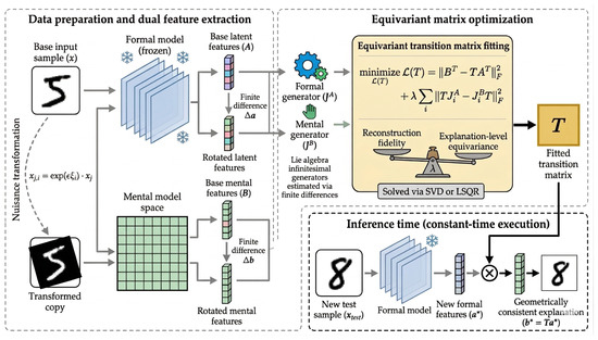
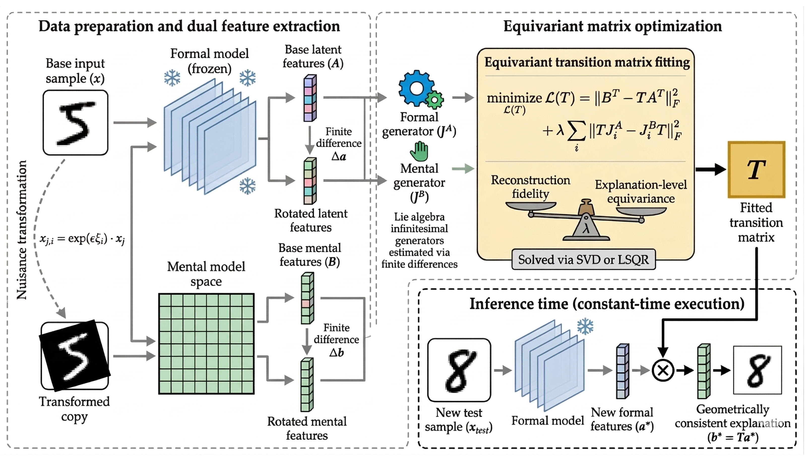
Conceptually, the formalization of a transition matrix [14] represents a mechanism for explanatory compression rather than complete mechanistic identity. The FM often contains numerous latent directions that are highly predictive but lack direct interpretability, whereas the MM retains only semantically inspectable coordinates. Consequently, a robust transition matrix acts as a stable decoding mechanism. While low fidelity error ensures accurate static reconstruction, it does not guarantee that explanations will behave coherently under input transformations. This critical requirement is achieved strictly through ETM’s novel equivariance constraints. Therefore, the shared-symmetry assumption is approximate and task-dependent, necessitating only a locally compatible first-order transformation law on the explored feature space. We introduce diagnostics to test this specific condition; if residuals ( and ) show disparities, practitioners can identify whether the transformation breaks down within the specific feature spaces or within the explainer itself. Figure 1 summarizes the proposed idea, showcasing how the training-stage generator estimation connects to the inference-stage explanation step.
Figure 1.
Overview of the ETM workflow. Paired FM and MM features are extracted from the same samples and from small transformed copies. Infinitesimal generators are estimated in both spaces, after which ETM fits a single transition matrix T that balances reconstruction fidelity and explanation-level equivariance. The same fitted matrix is then used at inference time without retraining the base model.
For practical implementation, the most defensible strategy for group selection relies on semantic meaning rather than pure algebraic convenience. Practitioners must initially identify transformations that preserve the underlying explanatory content from a user’s perspective. For example, small in-plane rotations serve as logical nuisance transformations for centered handwritten digits, whereas rigid 3D objects might require the special orthogonal group or the special Euclidean group . Only after nominating a candidate family based on domain knowledge should one estimate generators and inspect the diagnostic residuals to verify a credible local linearization in both FM and MM coordinates. Ultimately, ETM ensures that explanations remain robust and geometrically consistent by explicitly enforcing these domain-specific transformation rules.
3.1. Formalization of the Problem
Let denote the FM feature matrix extracted from a trained neural network, and let denote the corresponding MM feature matrix comprising expert-readable semantics. For a given sample x, the corresponding column vectors are defined as and . The transition matrix acts as a linear operator mapping FM features to MM features:
The linear formulation in Equation (1) is intentional. If an MM requires a highly nonlinear explainer, that MM is arguably misaligned with the primary explanatory purpose of the application. Therefore, ETM maintains the linearity of the explainer and embeds the geometric complexity within the transformation law, rather than within the surrogate model itself.
Assume that a Lie group G acts locally on the sample space X:
and that the induced FM and MM representations of Equation (3) are approximately equivariant:
The desired explanation map should approximately intertwine the two representations. Equations (2)–(4) introduce the object-level action and the induced FM and MM representations that motivate this essential requirement:
Let represent the Lie algebra of G, and let serve as a basis of infinitesimal generators. Denote by and the corresponding local linear actions within the two feature spaces. Differentiating Equation (5) yields the first-order intertwining condition:
In practical scenarios, the matrices and are estimated from small, transformed copies of each sample. For each data point and each symmetry direction , we generate
and approximate the local response using finite differences:
Equations (7) and (8) define the transformed copies alongside their corresponding finite-difference responses. The generator estimation step subsequently enforces the local linear response model defined in Equation (9). Specifically, this step solves:
A practical concern is that the symmetry hypothesis may fail when applied to real-world data. ETM should not be deployed blindly if the selected group fails to act coherently across both spaces. Therefore, diagnostic residuals must be computed following generator estimation. Let and denote the matrices formed by stacking the row-wise finite differences for generator i. We define these residuals as follows:
Small values for and indicate that the local linearization provides informative geometric constraints. In multi-generator settings, we additionally verify whether the estimated generators approximately satisfy the expected commutator relations. If these diagnostic metrics reveal poor alignment, the user should consider selecting a smaller regularization weight , reducing the transformation range, or entirely rejecting the symmetry hypothesis.
The selection of G must be driven by domain semantics rather than mathematical convenience. Appropriate groups typically correspond to nuisance transformations that preserve the core meaning of the explanation. Examples include planar rotations for centered handwritten digits, rigid motions for 3D point clouds, or scanner pose adjustments in image-guided medical systems. A candidate group is deemed acceptable only if it can be applied consistently to the raw object and if the resulting diagnostic residuals in Equation (10) remain small in both the FM and MM spaces.
As an illustrative example, consider the application of planar rotations utilized throughout the synthetic benchmark. Equation (11) defines the rotation group, Equation (12) outlines its action on the plane, and Equation (13) presents the canonical Lie-algebra generator:
acting on by
Its Lie algebra is generated by
If the FM and MM features maintain approximate equivariance with respect to this action, we can substitute and the rotation operator directly into Equations (3) and (4) to obtain the specific induced representations. Furthermore, because is generated by a single element , the corresponding spatial differentials are defined without the index i as:
Consequently, the general infinitesimal consistency condition from Equation (6) conceptually simplifies to the single, index-free intertwining relation .
3.2. Combined System and Scalable Solution
To optimally balance static reconstruction fidelity and transformation consistency, we formulate the transition matrix learning as the following minimization problem:
where balances fidelity and equivariance.
Using the Kronecker identity and letting , the fidelity term becomes:
while each symmetry block evaluates to:
For low-dimensional systems, the exact solution is computed via SVD, with the factorization and subsequent pseudoinverse operations detailed in Equations (19) and (20):
followed by the Moore–Penrose pseudoinverse:
For high-dimensional systems, explicitly constructing M is computationally prohibitive. Instead, our public implementation uses the LSQR algorithm with an implicit linear operator. Reshaping a vector v into matrix allows for the efficient computation of matrix–vector products, as formulated in Equation (21), without materializing massive Kronecker blocks.
The implicit formulation by Equation (21) bounds the per-iteration computational complexity according to Equation (22) defined by
and the memory footprint is naturally dominated by A, B, and the generators, rather than M.
Our MNIST implementation efficiently solves a system with unknowns using an implicit LSQR solver (, absolute and relative tolerances strictly set to , maximum 200 iterations). In the reference execution, convergence occurs in 127 iterations () taking 47.3 s on a CPU. These metrics confirm the pipeline’s tractability for medium-sized layers while keeping inference-time explanatory costs completely unchanged.
Because labeled validation sets are often unavailable in practice, we avoid treating as a black-box tuning parameter. For a dynamically fitted solution , we explicitly define two tracking ratios:
A practical, unsupervised selection rule involves locating the knee of the discrete L-curve defined by , or selecting the smallest that reduces below a target tolerance without significantly degrading . In our experiments, sweeping consistently identifies as the optimal operating point where symmetry improvements persist while fidelity gains saturate.
Equation (18) clarifies this regularization: the fidelity block represents empirical data constraints, whereas the symmetry blocks enforce structural constraints dictated by the chosen group action. Increasing shifts authority from data fitting to structure preservation. In small-scale settings, this trade-off alters the identifiable parameter directions in M’s singular spectrum; in large-scale scenarios, it impacts iteration counts, condition-number estimates, and the geometric shape of the L-curve. Combining solver diagnostics with the knee-point heuristic ensures the robust, principled calibration of .
Crucially, this unsupervised tuning is viable even without labeled validation splits during the explanation phase. Both evaluation components in Equation (23) are fully observable: is computed from paired FM and MM samples, and is derived from the estimated generators. The fundamental requirement is sufficient paired explanatory data, rather than external labels. Thus, the ETM layer can be rigorously calibrated on an entirely unlabeled explanation dataset while the backbone predictive model remains fixed.
3.3. Algorithm for Obtaining the Extended Transition Matrix
Algorithm 1 is deliberately lightweight, completely avoiding adversarial inner loops, FM retraining, or iterative MM refinement. Its only computationally intensive step is the one-time global resolution of the matrix T. Subsequently, generating explanations operates in constant time, offering a significant practical advantage over perturbation-based mechanisms. For high-volume, real-time deployments, this amortized computational cost is crucial. Like the broader transition-matrix family, ETM intrinsically leverages this highly efficient, amortized structure.
| Algorithm 1 Computation of the Equivariant Transition Matrices |
| Require: FM matrix and MM matrix Require: Generators and Require: Weight , truncation threshold , LSQR limit up to iterations Ensure: Transition matrix
|
The algorithm also highlights critical areas requiring strict numerical precision. To maintain a mathematically sound LSQR solver, the adjoint operator must perfectly mirror the implicit forward operator. Additionally, consistent generator normalization is required to ensure the symmetry penalty maintains a stable scale across independent executions. Finally, strict truncation thresholds are necessary to prevent noise-dominated singular directions from destabilizing the solution. Although these requirements do not alter ETM’s foundational mathematics, they are vital for ensuring empirical reproducibility.
Conceptually, Algorithm 1 reinforces that ETM is not a novel predictive model, but rather a geometrically constrained explainer strictly fitted to paired FM and MM features. Once T is computed, the inference stage becomes remarkably inexpensive: for any new FM feature vector , the corresponding interpreted MM prediction is simply given by .
3.4. Experimental Framework and Evaluation Setup
We selected two primary benchmarks to expose the complementary strengths and weaknesses of our method. The synthetic setting acts as an identifiability microscope: its intentionally small scale allows for the direct inspection of matrices, the visualization of generators, and a clear understanding of ’s effect without confounding architectural complexity. Conversely, MNIST stresses dimensionality, numerical solver behavior, and qualitative explanation usability. Together, these benchmarks demonstrate how ETM modifies the operator when symmetry is the sole additional ingredient in a controlled environment.
While two benchmarks alone cannot definitively establish universal generality, we provide supplementary analyses (see Section S7 in the Supplementary Materials), including a known-generator benchmark, an multi-generator analysis, and a brief discussion on point cloud scalability. Although not a complete multi-modal suite, these additions confirm that the ETM formulation is not restricted to a single dataset or a one-parameter example. The synthetic and MNIST studies serve as the main narrative because they maintain comprehensibility.
Consequently, we evaluate ETM in two scenarios designed to separate mathematical controllability from practical scale. The synthetic benchmark allows direct inspection of the transformation structure, while the MNIST benchmark utilizes raw pixel space as the MM. To address potential concerns regarding limited scope, our auxiliary studies in the Supplementary Materials test whether the formulation remains robust when the group action is known exactly or when multiple generators are enforced.
3.4.1. Research Protocol on Synthetic Data
The synthetic benchmark is intentionally didactic. Because the matrices are explicitly reproduced in Appendix A, readers can easily verify dimensions, inspect baseline fits, and directly connect numerical outputs to the algebraic formulation. This transparency is challenging to achieve with larger datasets. The small scale proves that ETM does not require massive sample counts to enforce the symmetry prior; the prior acts purely on the operator via the generators, rather than relying on a high-capacity nonlinear parameterization.
A limitation of this protocol is the proxy-space construction. Because rotations are defined after MDS projection, this experiment represents a controlled stress test of explanation geometry rather than a natural object-level group action. We address this limitation by quantifying embedding and back-projection distortion in the Supplementary Materials, reporting stability across multiple projection methods, and including a known-generator benchmark that demonstrates ETM’s qualitative advantage without the MDS bridge. These clarifications strengthen the study’s methodological value without overstating its conclusions.
The synthetic protocol utilizes paired samples, with the FM matrix and the MM matrix explicitly provided in Equations (A1) and (A2) of Appendix A. Additionally, the exact baseline transition matrix used for comparisons is documented in Equation (A3). Since these vectors lack a canonical geometric action, applying direct rotation in the original ambient coordinates would be arbitrary. Instead, we use a two-dimensional MDS embedding as a proxy object space where planar rotation is well-defined. This embedding induces a consistent local rotation field necessary for a controlled diagnostic experiment.
Because this proxy construction can introduce pairwise-distance distortion and linear decoder reconstruction errors, we track both effects. For the released benchmark, the relative pairwise-distance distortions are 1.87% for A and 1.34% for B, with back-projection residuals of 8.82% and 9.13%, respectively. These metrics confirm that the MDS bridge is sufficiently faithful for first-order generator estimation. The known-generator experiment in the Supplementary Materials further ensures that the main conclusions are not merely proxy artifacts.
Algorithm 2 summarizes the generator-estimation procedure. Applying this to both A and B produces a pair of generators, and , representing the identical external symmetry across two different feature spaces. The heatmaps of these estimated infinitesimal generators are visualized in Figure A1 of Appendix B.
| Algorithm 2 Obtaining Generator via 2D Rotation |
| Require: Source feature matrix (or MM matrix B) Require: Embedding method (Metric MDS), perturbation angle (e.g., rad), Ridge regularization parameter Ensure: Infinitesimal generator matrix
|
|
|
The synthetic configuration, defined in configs/synthetic.yaml, sets , , , uses a fixed MDS random state of 42, and evaluates robustness across angles from to in increments.
3.4.2. Research Protocol on MNIST Dataset
The MNIST architecture is kept intentionally simple to ensure ETM’s explanatory contribution is not obscured by a highly complex FM. A two-convolution network with a 490-dimensional penultimate layer provides a rich latent code while ensuring transition matrix tractability. Using raw pixel space as the MM makes the explanations highly concrete, as users directly interpret reconstructed digit images rather than abstract concept bases. While pixel-space MMs are advantageous for visual comparison here, concept-space alternatives and their associated dimensionality trade-offs are discussed in the Supplementary Materials (see Section S9).
The image-rotation protocol highlights that ETM requires reliable local tangent estimates, not large-amplitude transformations during fitting. Small symmetric finite differences are preferred over aggressive data augmentation because the goal is to approximate the Lie algebra action, not to train a robust predictor. ETM relies on transformed samples strictly to estimate derivatives of the explanation geometry.
The benchmark utilizes the standard 60,000/10,000 MNIST split [26]. The FM is a lightweight CNN with a penultimate dimension of . The released implementation consists of two convolutional layers (32 and 64 channels), two max-pooling operations, dropout (), a fully connected 490-dimensional layer, and a 10-class output. Since the MM is raw pixel space, .
The backbone is trained using Adam (learning rate , batch size 256, weight decay 0) for five epochs with seed 42 on a CPU. Consequently, remains the only ETM-specific hyperparameter actively swept, enhancing reproducibility and distinguishing explainer design from model design.
For generator estimation, rotations use a differentiable affine transformation with bilinear interpolation and zero padding. The repository computes central finite differences using a small angular step. The exact same routine is applied to both FM and MM spaces to maintain internally consistent generator estimates, heavily emphasizing local tangent behavior over extreme image reconstruction.
3.4.3. Experiment Methodology and Scenarios
The evaluation is structured into three scenarios. Scenario 1 establishes an exact fidelity-only baseline, preventing hidden improvements from confounding the results. Scenario 2 isolates the symmetry penalty’s effect through the sweep. Crucially, Scenario 3 shifts focus from static fit quality to behavioral coherence, testing whether explanations remain robust when inputs undergo transformations beyond the nominal fitting condition. This final test is vital, as many methods perform well on static metrics but fail to produce a related family of explanations for a related family of inputs.
Specifically, Scenario 1 utilizes the baseline objective from Equation (24):
Scenario 2 fits ETM using the combined objective in Equation (15). Scenario 3 evaluates robustness under larger rotations; the synthetic study uses rotated trajectories in the proxy object space, while the MNIST study rotates test digits from to and reconstructs them using both the baseline and ETM.
3.4.4. Evaluation Criteria and Metrics
The metrics encompass three complementary perspectives. Fidelity metrics assess whether the MM can be reconstructed. Symmetry metrics verify whether the explanation respects the designated transformation law. Robustness metrics evaluate graceful degradation as inputs deviate from fitting conditions. No single metric is sufficient; an explainer might achieve high similarity index but poor symmetry defect, or vice versa.
While we report standard deviations, confidence intervals, and bootstrap summaries to quantify empirical fluctuation, these do not provide a calibrated posterior over the explanation operator. We emphasize this distinction to prevent over-interpretation of narrow confidence intervals as proof of epistemic certainty in high-stakes environments.
Fidelity on the synthetic benchmark is evaluated via mean squared error (MSE) by Equation (25).
For MNIST, we measure Structural Similarity Index (SSIM) and Peak Signal-to-Noise Ratio (PSNR) as defined in Equations (26) and (27), respectively.
The symmetry defect (SymDef), representing the Frobenius norm of the commutator mismatch, is defined in Equation (28):
and normalized across scales in Equation (29):
where NSD stands for normalized symmetry defect.
Robustness under transformation is quantified by the performance drop between the canonical orientation and the worst tested angle, which is calculated using Equation (30).
Because ETM is deterministic once A, B, and the generators are fixed, the reported uncertainty strictly reflects the empirical variability of the evaluation metrics, not a posterior distribution over T.
4. Results
The empirical outcomes must be evaluated at two complementary levels. Numerically, the ETM is successful if it reduces the Lie-algebraic commutator mismatch without compromising reconstruction fidelity. Qualitatively, it is successful if the resulting visual explanations vary under continuous transformations in a coherent manner that humans can parse as transformation-consistent. We combine metric tables with trajectory visualizations, reconstructed panels, and distribution plots to address the practical concern that a small SymDef is only valuable if it translates into coherent explanations.
We answer three practical questions: (Q1) can ETM sharply reduce the SymDef, (Q2) does this reduction preserve reconstruction quality, and (Q3) do explanations become qualitatively more usable under transformations?
4.1. Synthetic Test: Controlled Trade-Off of Accuracy and Equivariance
The synthetic findings illustrate how ETM modifies the explanation operator before introducing high-dimensional image complexity. Since the baseline matrix already fits the paired samples well, the large drop in SymDef is not merely a side effect of better optimization. Instead, the geometry of the fit changes. The ETM solution aligns with the learned generators, stabilizing the rotated trajectory. Explanation-level symmetry can thus be strongly enforced even with few samples, provided the generators are informative.
To ensure these conclusions do not rely on a single projection technique, we evaluate multiple low-dimensional diagnostics: PCA for linear variance [46], MDS for pairwise dissimilarities [47], t-SNE for local neighborhoods [48], and UMAP for manifold connectivity [49]. ETM behaves consistently across all four methods. This cross-method agreement confirms our qualitative interpretation: ETM keeps transformed explanations closer to the ideal MM trajectory than the baseline.
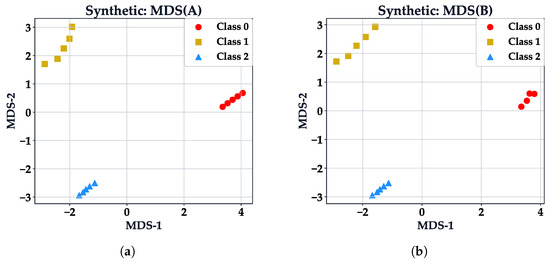
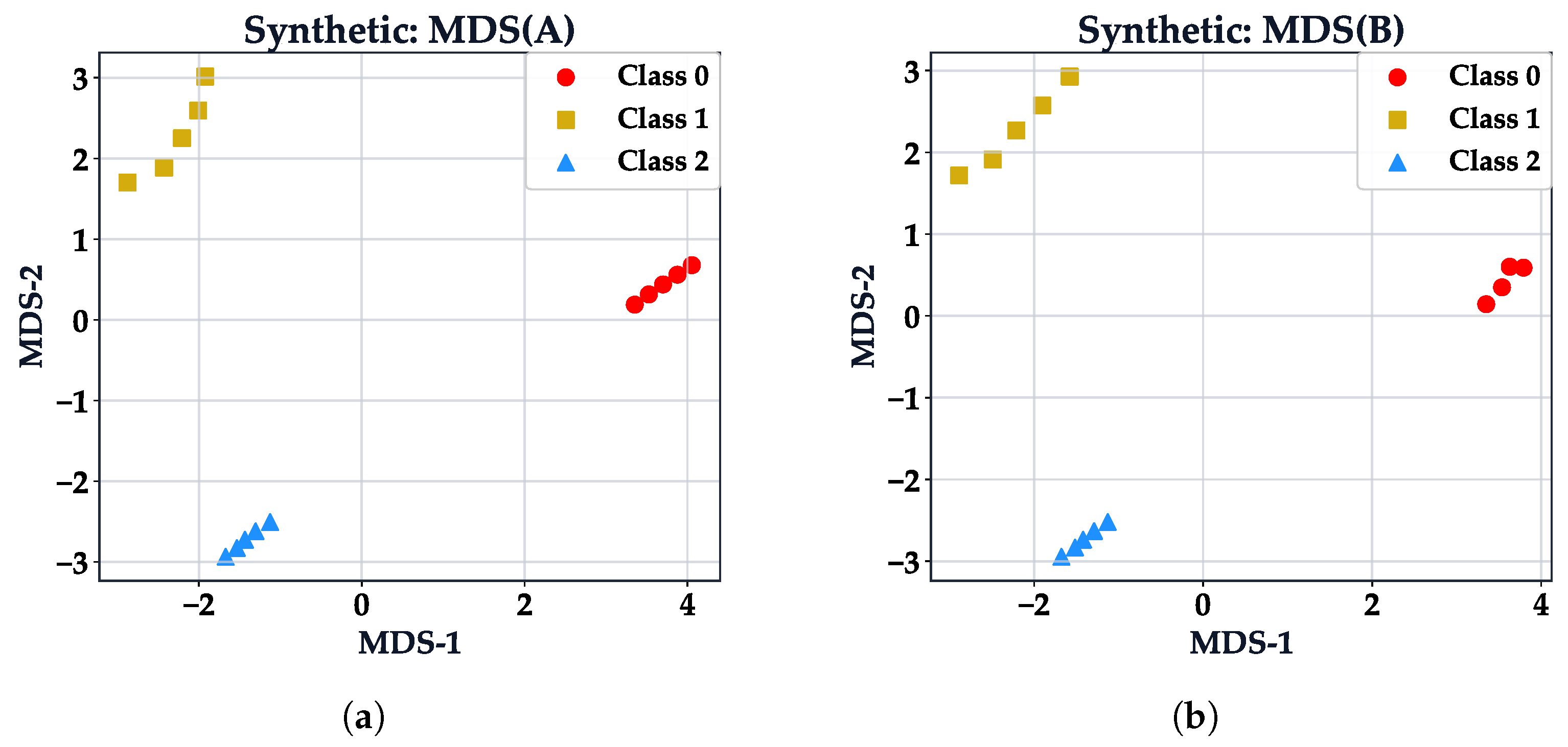
Figure 2 shows the proxy geometry for the synthetic study. The MDS embeddings of A and B are topologically similar but not identical, making the transition problem non-degenerate. The baseline matrix relies on fidelity-only Least Squares, while ETM incorporates the infinitesimal commutation constraint.
Figure 2.
Visualization of the synthetic feature spaces using MDS. (a) The FM feature space , representing abstract latent representations. (b) The MM interpretable feature space .
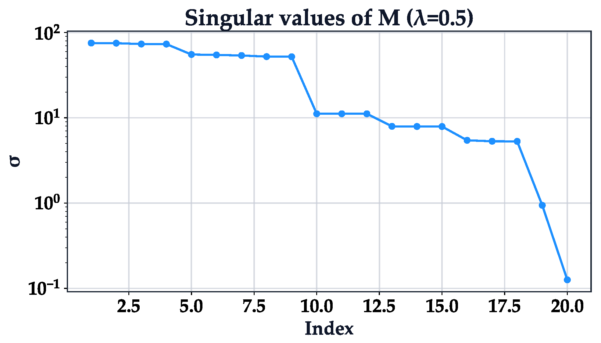
The results in Table 1 show that even with a moderate increase in MSE, a linear matrix T with equivariant regularization provides sufficient accuracy. The central result is the collapse of the SymDef by over five orders of magnitude, from to , while MSE increases marginally from 0.00367 to 0.00524. This confirms that the complexity of the connection between spaces A and B in our experiments is successfully resolved through considering data geometry rather than complicating the transition operator itself. The numerical stability of this solution is further evidenced by the singular value spectrum of the system matrix M, shown in Figure A2 (Appendix B), which displays a smooth decay without catastrophic drops in the relevant rank range.
Table 1.
Synthetic test: Comparison of accuracy and equivariance between the baseline and the proposed approach. Arrows (↓) indicate that lower values denote better performance. The best results for the SymDef and NSD are highlighted in bold. Standard errors are computed via bootstrap resampling with 1000 iterations.
Overall, this improvement represents a genuine structural shift toward approximate intertwiners. The Supplementary Materials confirm that this holds in a known-generator benchmark requiring no MDS proxy.
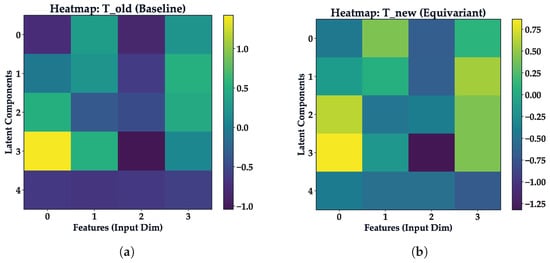
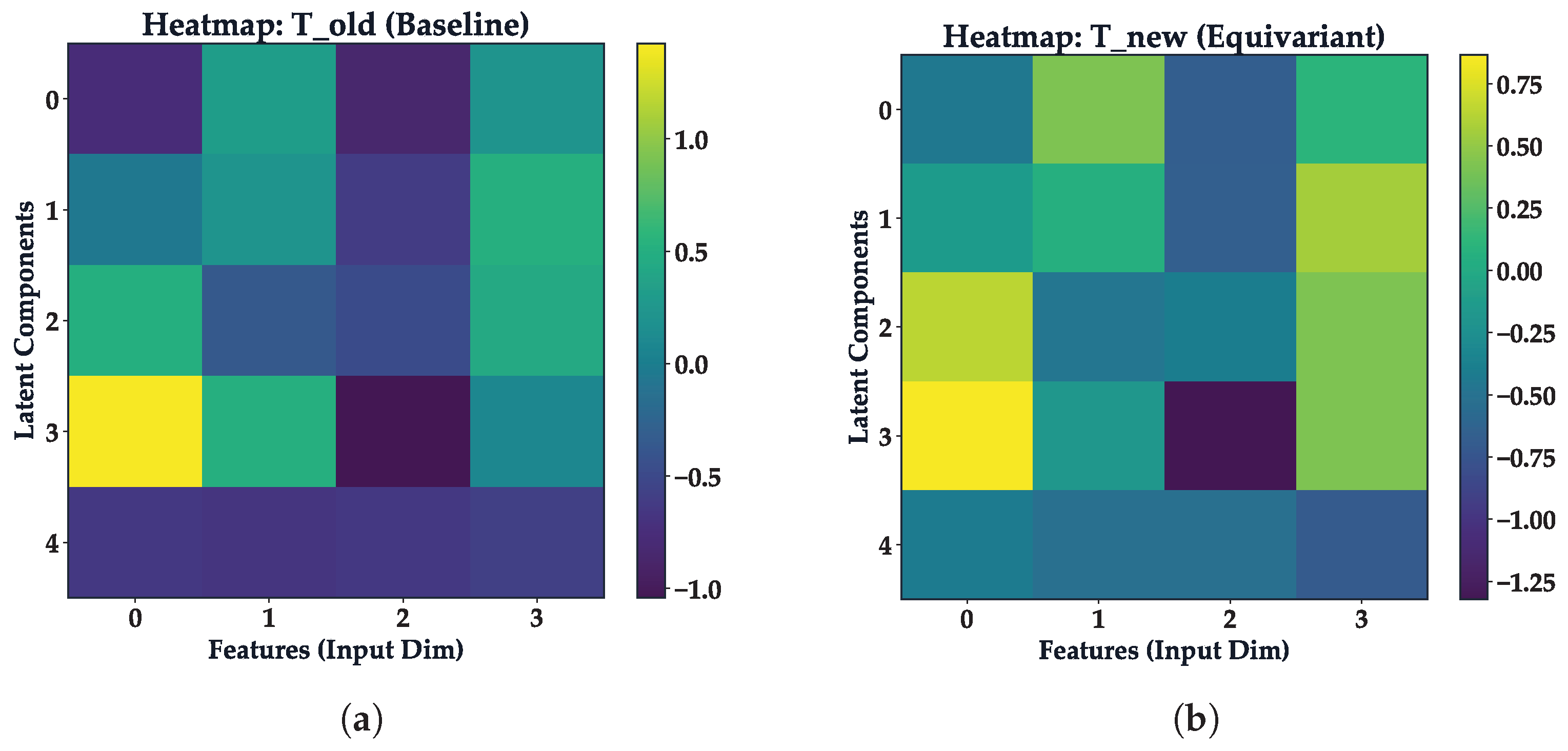
The heatmaps in Figure 3 demonstrate the qualitative impact of the commutator penalty. ETM does not simply shrink the baseline matrix; it reorganizes the mapping so transformed FM directions target compatible MM directions. Practically, a nuisance rotation no longer causes chaotic MM coordinate drift.
Figure 3.
Comparison of synthetic transition matrices. (a) Baseline matrix obtained by minimizing only reconstruction error (MSE). (b) ETM obtained with , exhibiting a structured pattern.
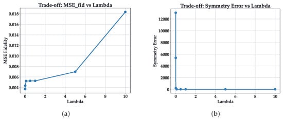
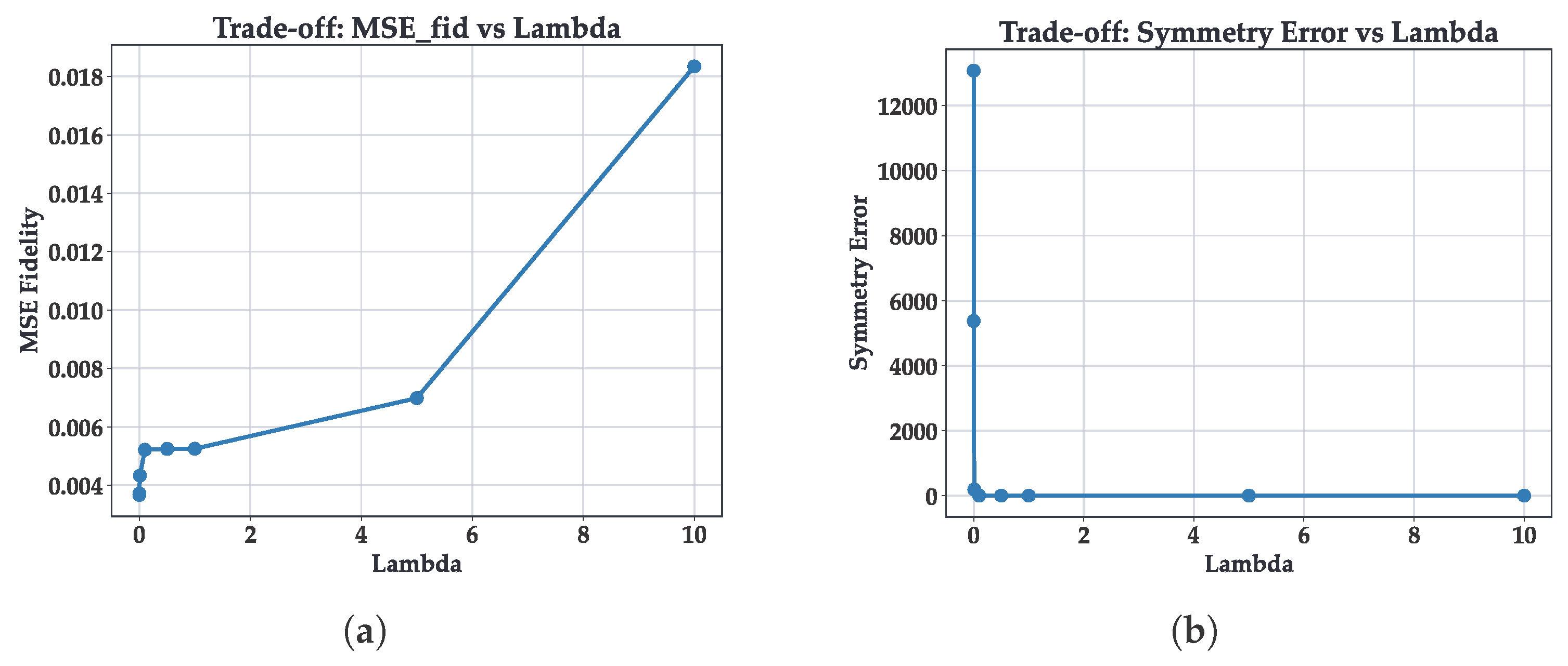
Figure 4 complements Table 2, which clarifies the selection of the regularization parameter . The sharpest symmetry drop occurs between and , while improvements beyond yield diminishing returns relative to MSE increases. This behavior justifies the knee-based heuristic in Equation (23) and establishes as a robust operating point.
Figure 4.
Trade-off analysis between reconstruction fidelity and symmetry preservation for varying regularization weights . (a) MSE shows a gradual increase as structural constraints tighten. (b) SymDef demonstrates a reduction by several orders of magnitude.
Table 2.
Synthetic test: Sensitivity analysis of the regularization parameter . The table demonstrates the trade-off between reconstruction accuracy (MSE) and the SymDef magnitude.
Finally, Figure A3 in Appendix C confirms that ETM trajectories remain highly stable across visualization methods (PCA, MDS, t-SNE, and UMAP), demonstrating that the observed robustness is intrinsic to the optimized mapping and not an artifact of a specific projection.
4.2. MNIST Test: Equivariant Explanations from Deep Features
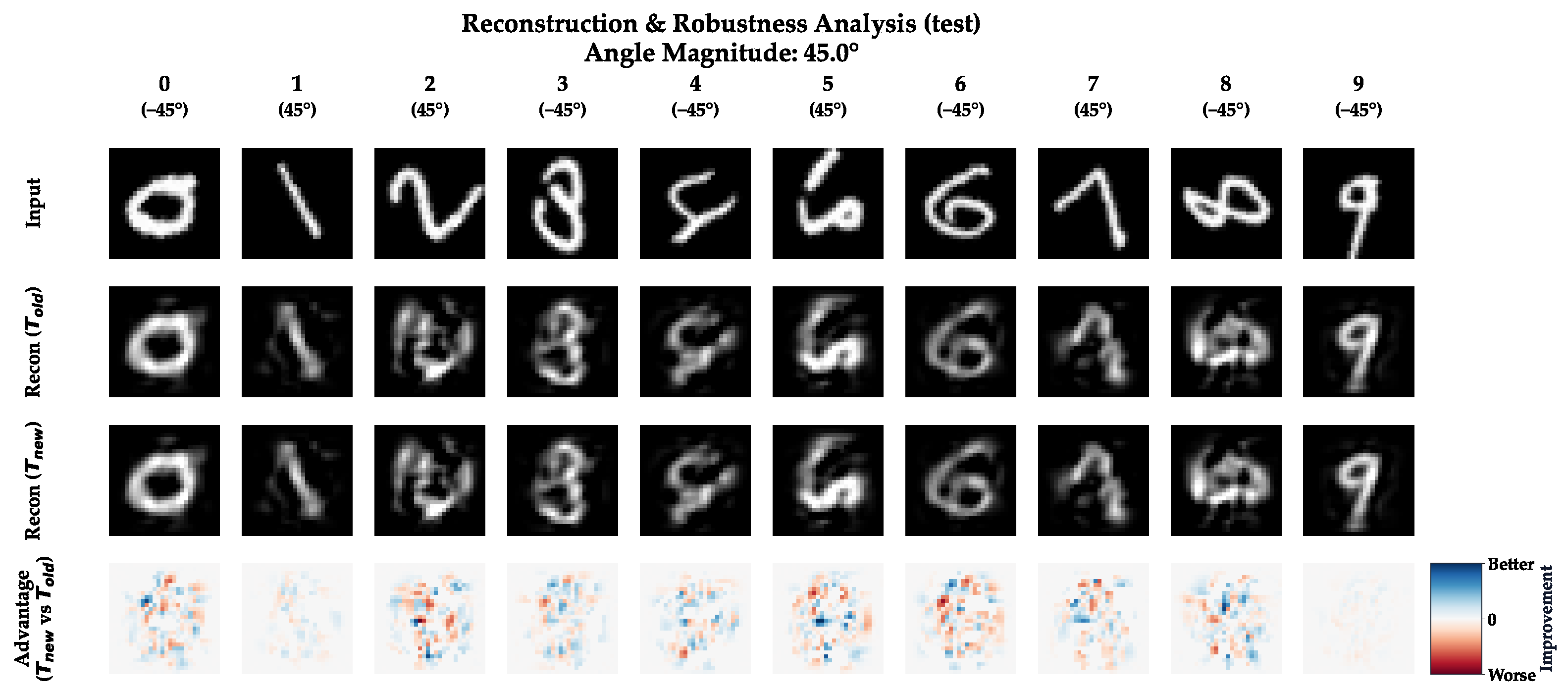
On MNIST, the crucial outcome is not that ETM reconstructs slightly sharper digits—baseline fidelity is already high—but that ETM alters the reconstruction error pattern. Under input rotation, the baseline often misplaces structurally significant elements, like loop curvature or stroke terminals. ETM preserves these global shape relations, dispersing remaining errors into semantically less-disruptive regions. For users, this means that the explanation visually remains a transformed version of the original digit rather than a corrupted alternative, even if SSIM changes are minute.
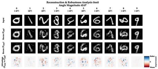
The MNIST experiment tests if this logic holds when generators are numerically estimated from real images rather than synthetic proxies. Figure 5 displays reconstructions at a rotation. The ETM reconstructions preserve digit topology more faithfully in regions such as stroke tips, loop closure, and centroid placement, while the baseline exhibits more local artifacts in these structurally important areas. Extended qualitative comparisons of reconstructions at boundary rotation angles are provided in Figure A5 (Appendix D).
Figure 5.
Qualitative comparison of reconstructed MNIST explanations at . The figure displays the Input image, Baseline reconstruction (), ETM reconstruction (), and the difference maps (Advantage).
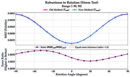
Figure 6 complements Figure 5, showing that ETM produces a smoother angle-dependent error curve. The baseline frequently concentrates errors on vital structures, like the open tip of a “5” or the loop of an “8”. ETM diffuses this error, minimizing shape destruction. For end-users, transformation-induced variations are correctly attributed to input rotation rather than explainer instability. To further validate this structural stability, additional visualizations and displacement vector fields are detailed in Figure A6 (Appendix E).
Figure 6.
Evolution of MSE across rotation angles . ETM closely tracks the baseline fidelity while exhibiting a more regular error profile across the full rotation range.
Table 3 gathers central MNIST indicators in one place. ETM reduces the SymDef by 72.6% with negligible fidelity loss. The absolute change in test SSIM is approximately 0.0002 and PSNR is 0.0088 dB. These minor differences relative to test set standard deviations confirm that geometric consistency can be enforced without sacrificing spatial baseline fidelity.
Table 3.
MNIST: Fidelity and symmetry metrics on training and test sets. SSIM and PSNR (in decibels, dB) are reported as mean ± standard deviation; confidence intervals correspond to the mean under a normal approximation. Arrows indicate the direction of better performance (↑ higher is better; ↓ lower is better).
Algorithmic scalability is also preserved. The ETM constraint alters how the transition matrix T is fitted, not how explanations are generated during inference. Explaining a novel image still requires exactly one FM forward pass and one matrix multiplication, preserving the constant-time deployment advantage of transition-matrix explainers.
A detailed computational performance analysis for the MNIST-scale experiment, including runtime metrics, memory profiling, and condition number estimates, is provided in the Supplementary Materials (see Section S8).
4.3. Comparison with Post Hoc Baselines
Comparing the proposed ETM against baselines like LIME [4], Integrated Gradients [5], and SHAP [6] requires careful methodology. Because these tools emit localized attributions while ETM reconstructs global explanations within an MM space, we evaluate them based on deployment costs and structural guarantees rather than assuming identical optimization targets. ETM’s closest analog is the standard fidelity-only transition matrix. Therefore, direct comparison is optimal for positioning ETM within the explainer design space rather than asserting dominance across incomparable outputs.
Analyzing ETM alongside robust post hoc methods is also conceptually insightful. Adversarial stabilization, Bayesian surrogates, and manifold-aware Shapley values all strive to minimize spurious variability in local explanations. While sharing this goal, ETM operates in a mechanistically different way by enforcing a first-order commutation law between feature spaces instead of relying on local resampling. Consequently, ETM can readily complement local-robustness methods. Because direct numerical evaluation is only straightforward against the fidelity-only baseline, we utilize two comparison formats: a quantitative assessment against the direct baseline (Table 4), and a structural/computational comparison across broader post hoc families (Table 5).
Table 4.
Direct comparison between the fidelity-only transition matrix and ETM.
Table 5.
Comparison of ETM with representative post hoc and architecture-level explanation families. The cost column refers to the typical effort needed per explanation once the base model has been trained.
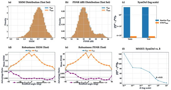
To comprehensively contextualize these results, Figure 7 summarizes ETM’s statistical performance on the MNIST dataset. The extensively overlapping SSIM and PSNR distributions confirm that ETM avoids catastrophic failures. Concurrently, the distinct separation in SymDef magnitude highlights a fundamental structural transformation in the operator. ETM globally refines the explanation law without sacrificing difficult samples, ensuring robust geometric coherence across the entire data distribution.
Figure 7.
Quantitative performance summary on the MNIST dataset. (a,b) Distributions of SSIM and PSNR for Baseline and ETM, showing comparable reconstruction quality. (c) SymDef for training and test sets, highlighting the notable reduction achieved by ETM. (d,e) Robustness curves for SSIM and PSNR across rotation angles. (f) Impact of the regularization parameter on the SymDef, illustrating the control over geometric consistency.
Although ETM’s primary advantage is structural, confirming its reconstruction stability remains essential. Table 6 details stability statistics across an extended test range (). The observed performance differences are negligible and consistently non-catastrophic, proving that enforcing equivariance does not introduce systemic brittleness.
Table 6.
MNIST: Robustness summary on an extended test range (). “Drop” is defined as the difference between the metric value at the standard orientation () and the minimum value observed over the rotation range, i.e., .
Table 7 demonstrates a monotonic decrease in SymDef as increases. We select as an optimal operating point that achieves substantial symmetry reduction without visually compromising the reconstructed accuracy.
Table 7.
MNIST: Impact of the hyperparameter on the SymDef and solver characteristics. Solver diagnostic columns (Least Squares iterations, residual norm , and estimated condition number ) are provided for the regularized solution.
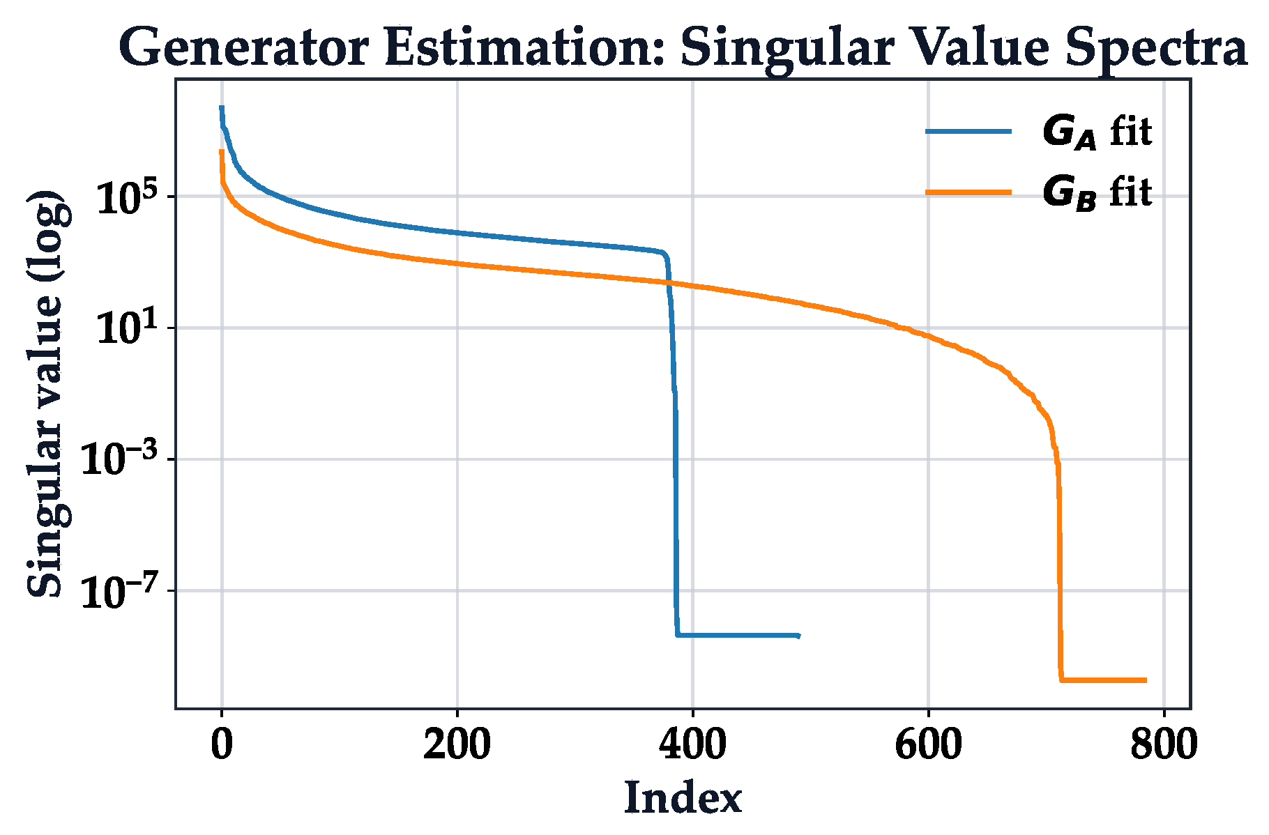
Crucially, Table 7 also details Least Squares iterations and conditioning estimates. Because the equivariance constraint effectively couples numerous degrees of freedom through the commutator, poor conditioning could destabilize the optimization. Fortunately, the moderate iteration counts confirm computationally efficient resolutions. Furthermore, Figure A4 in Appendix C reveals long tails in the singular-value spectrum for the generator estimation problems. This underscores the necessity of regularization to truncate noise and yield stable differential operators. Together, these diagnostics prove that ETM securely solves a well-posed constrained regression problem in a numerically sound regime.
While our primary narrative focuses on a continuous one-parameter transformation group for transparency, the Supplementary Materials expand this analysis extensively. By incorporating a known-group benchmark, a multi-generator setting, and a 3D point-cloud scenario, we demonstrate that ETM’s underlying mathematical formulation translates smoothly beyond simplified pixel domains.
Furthermore, this work situates ETM firmly within the broader literature motivating its design, bridging GDL, classical dimensionality reduction, and robust numerical solvers [24,25]. Finally, Appendix B supplies additional diagnostic materials, including generator heatmaps, cross-embedding stability plots, and extended generative reconstructions, enabling deeper visual inspection of the core operator geometry.
5. Discussion
The empirical evaluations detailed in Section 4 confirm that the proposed ETM significantly alters the mathematical geometry of the explanation operator without materially degrading the underlying reconstruction fidelity. This operational behavior aligns fundamentally with the theoretical intertwining constraints formulated in Section 3. Traditional fidelity-only transition matrices, bounded by Equation (24), merely map static pointwise feature pairs. In contrast, ETM concurrently learns to map these pairs and their local transformation laws. In the synthetic experimental benchmark, summarized in Table 1 and Figure 4, the method actively projects the baseline solution toward a space of approximate intertwiners. This optimization shrinks the SymDef by multiple orders of magnitude while preserving geometric stability. Furthermore, as demonstrated in the MNIST benchmark and corroborated by the comprehensive qualitative visualizations in Figure 7, this mechanism robustly survives even when the corresponding infinitesimal generators are estimated numerically directly from image data, yielding a 72.6 percent symmetry improvement with statistically negligible fidelity penalties.
Comparing these technical outcomes with existing frameworks established in Section 1 clarifies the unique methodological position of ETM. While Concept Bottleneck Models demand ground-truth semantic labels during the initial training phase [27], and local surrogates like BayLIME rely on iterative, computationally heavy perturbation sampling [7], ETM operates entirely post hoc as a global linear operator. Table 5 illustrates this fundamental distinction. ETM is not intended to replace architecture-level equivariant designs, such as group-equivariant convolutional networks [18,19], nor does it act as a substitute for training-time Jacobian regularization [21]. Instead, it offers a globally consistent, transformation-aware mapping tailored for already-trained networks. This provides a distinct computational advantage in highly regulated environments where the base FM cannot be feasibly retrained.
The primary algorithmic advantage of ETM stems from its scalable formulation, seamlessly alternating between SVD outlined in Equation (19) for low-dimensional systems and implicit LSQR algorithms for large parameter spaces. As specified in Algorithm 1, inference remains strictly constant-time, requiring exactly one forward pass and one matrix multiplication. However, an inherent disadvantage is the approach’s strict theoretical reliance on the assumption that both spaces admit approximately compatible local group actions. If the semantic MM lacks well-defined transformation behavior, incorporating the penalty defined in Equation (15) risks over-regularizing the explanation. Consequently, the operational diagnostic residuals formalized in Equation (10) are absolutely essential. Practitioners must systematically estimate these residuals and only retain symmetry hypotheses whose local linearizations prove empirically credible.
A further contextual disadvantage relates to the synthetic MDS proxy utilized in Section 3.4.1 and visualized in Figure 2. This mathematical bridge is a controlled construct explicitly designed to induce a continuous rotation field on abstract vectors. While the induced relative pairwise-distance distortion remains low, the embedding should not be misinterpreted as the true underlying data manifold. Beyond synthetic spaces, transferability introduces domain-shift complexities. In environmental deep learning, models must frequently transfer across geographic regions. In our setting, maintaining structural coherence across differing acquisition domains, medical scanners, or dynamic sensing conditions whose nuisance symmetries exhibit minor variations presents a highly promising vector for expanding ETM’s utility.
Addressing these scalability frontiers, applying ETM to 3D point-cloud modalities emerges as a particularly compelling extension. Modern point-cloud architectures inherently dedicate substantial effort to reconciling global context with precise local structural physics. Models like GPSFormer integrate transformer-style global reasoning [44], while DAF-Net utilizes dynamic acoustic-field fitting to model fine-grained geometry [45]. ETM could be strategically integrated on top of such learned structural features to decode them into human-auditable geometric descriptors, provided the chosen MM accommodates a stable, continuous rigid-motion action instead of raw coordinate structures.
Despite its documented empirical advantage, this approach retains notable limitations and faces several open research challenges that require dedicated future exploration. A primary shortcoming is that while ETM tracks the empirical variability of static fidelity metrics, it does not currently provide a calibrated spatial or pixel-level quantification of explanation uncertainty. While we successfully compute standard errors for scalar fidelity metrics via bootstrap resampling, developing techniques to refit the ETM objective on bootstrap resamples or ensemble backbone features to generate visual, pixel-wise uncertainty maps remains an unresolved challenge. Such probabilistic mapping would allow users to reliably distinguish structurally stable explanations from those weakly supported by paired observational data. Furthermore, applying the Lie algebra intertwining relations to richer, multi-generator symmetry groups, such as the special Euclidean group or the three-dimensional rotation group , poses a significant numerical challenge. Estimating stable generators for complex translations and rotations concurrently will require careful, domain-specific pipeline designs. Addressing these open questions through structured concept descriptors and advanced spatial benchmarks will be essential to advancing explanation-level equivariance.
6. Conclusions
In summary, this manuscript establishes a notable methodological shift in evaluating post hoc explanation maps, demonstrating that static reconstruction fidelity alone is insufficient for deploying interpretable deep learning in high-stakes environments. We introduce a novel approach called ETM to ensure that explanatory mappings preserve the geometric transformation logic relating similar inputs. This approach upgrades classical transition matrices into symmetry-aware operators without requiring computationally expensive retraining of the formal predictive network. By estimating infinitesimal generators across formal and mental feature spaces, ETM enforces an approximate intertwining relation directly at the Lie algebra level. Consequently, ETM retains the constant-time deployment advantages of linear explainers, requiring only one forward pass and one matrix multiplication during inference. Our evaluations confirm that this approach achieves profound structural improvements while preserving data reconstruction quality. On a controlled synthetic benchmark, ETM collapses the SymDef from 13,100 down to 0.0425, with only a marginal MSE penalty. Scaling to the MNIST dataset, the approach secures a 72.6 percent decrease in the SymDef, dropping from 141.19 to 38.65. Simultaneously, structural similarity and PSNR remain practically unaffected, varying by less than 0.03 and 0.06 percent, respectively. The resulting explanations reliably maintain interpretable topologies under continuous spatial transformations. Despite these advances, the methodology remains limited by the requirement for a valid, shared symmetry hypothesis across representation spaces, the sensitivity of generator estimation, and the linear nature of the explainer itself.
Future research directions will focus on developing calibrated uncertainty estimation protocols to dynamically flag unstable explanations, extending intertwining relations to accommodate multi-parameter transformation groups, and deploying structured MMs for complex structural domains such as three-dimensional geometry and point-cloud analysis.
Supplementary Materials
The following supporting information can be downloaded at: https://www.mdpi.com/article/10.3390/make8040092/s1, File Supplementary Material: “Equivariant Transition Matrices for Explainable Deep Learning: A Lie Group Linearization Approach.”
Author Contributions
Conceptualization, P.R., O.B., L.B. and I.K.; methodology, P.R. and O.B.; software, P.R.; validation, P.R., O.B. and L.B.; formal analysis, P.R., O.B., L.B. and I.K.; investigation, P.R.; resources, O.B. and I.K.; data curation, L.B. and I.K.; writing—original draft preparation, P.R. and O.B.; writing—review and editing, L.B. and I.K.; visualization, P.R.; supervision, I.K.; project administration, O.B. All authors have read and agreed to the published version of the manuscript.
Funding
This research received no external funding.
Institutional Review Board Statement
Not applicable. This study used publicly available datasets and did not involve humans or animals.
Informed Consent Statement
Not applicable. This study did not involve humans.
Data Availability Statement
Publicly available datasets were analyzed in this study. The MNIST dataset can be found in reference [26]. The synthetic data matrices used in the controlled experiment are reproduced in Appendix A. The source code, configuration files, generated matrices, and logs used to produce the reported experiments are available in the GitHub repository https://github.com/radiukpavlo/transition-matrix-etm-xai (accessed on 16 February 2026).
Conflicts of Interest
The authors declare no conflicts of interest.
Abbreviations
The following abbreviations are used in this manuscript:
| AI | Artificial Intelligence |
| ETM | Equivariant Transition Matrices |
| FM | Formal Model |
| GDL | Geometric Deep Learning |
| LSQR | Least Squares QR |
| MDS | Multidimensional Scaling |
| MM | Mental Model |
| MNIST | Modified National Institute of Standards and Technology |
| MSE | Mean Squared Error |
| NSD | Normalized Symmetry Defect |
| PSNR | Peak Signal-to-Noise Ratio |
| SSIM | Structural Similarity Index |
| SVD | Singular Value Decomposition |
| SymDef | Symmetry Defect |
| XAI | Explainable Artificial Intelligence |
Appendix A. Synthetic Data
This appendix reproduces the synthetic matrices used in the controlled benchmark. Equations (A1)–(A3) list the exact FM matrix, MM matrix, and fidelity-only baseline transition matrix used in the synthetic study. Because the transition matrix is defined in the main text as , the matrix printed below is the fidelity-only baseline in its transposed form , matching the orientation used in the public implementation.
Appendix B. Generator Visualizations and System Conditioning
Figure A1 groups the two estimated generator heatmaps used in the synthetic benchmark.
Figure A1.
Heatmaps of the estimated infinitesimal generators for the synthetic dataset (). (a) Generator representing the rotation action in the FM space. (b) Generator representing the rotation action in the MM space.
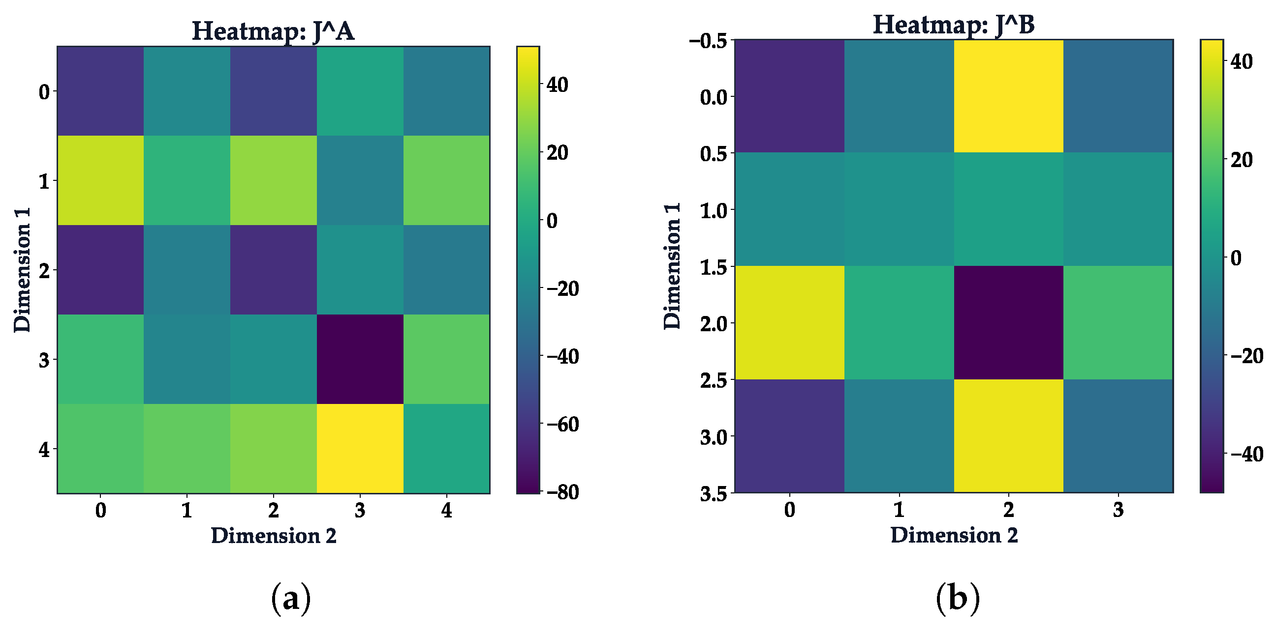
Figure A2.
Singular-value spectrum of the synthetic system matrix M for . The smooth decay indicates that the constrained Least-Squares problem is well behaved after truncation.
Appendix C. Additional Stability Embeddings
Figure A3.
Comparative visualization of representation stability under rotation using various dimensionality reduction techniques. (a) PCA, (b) MDS, (c) t-SNE, and (d) UMAP. Each plot overlays the trajectories of the static (ideal), baseline, and ETM-transformed features, demonstrating that the ETM (blue triangles) preserves the topological structure of the rotation manifold better than the baseline (orange squares).
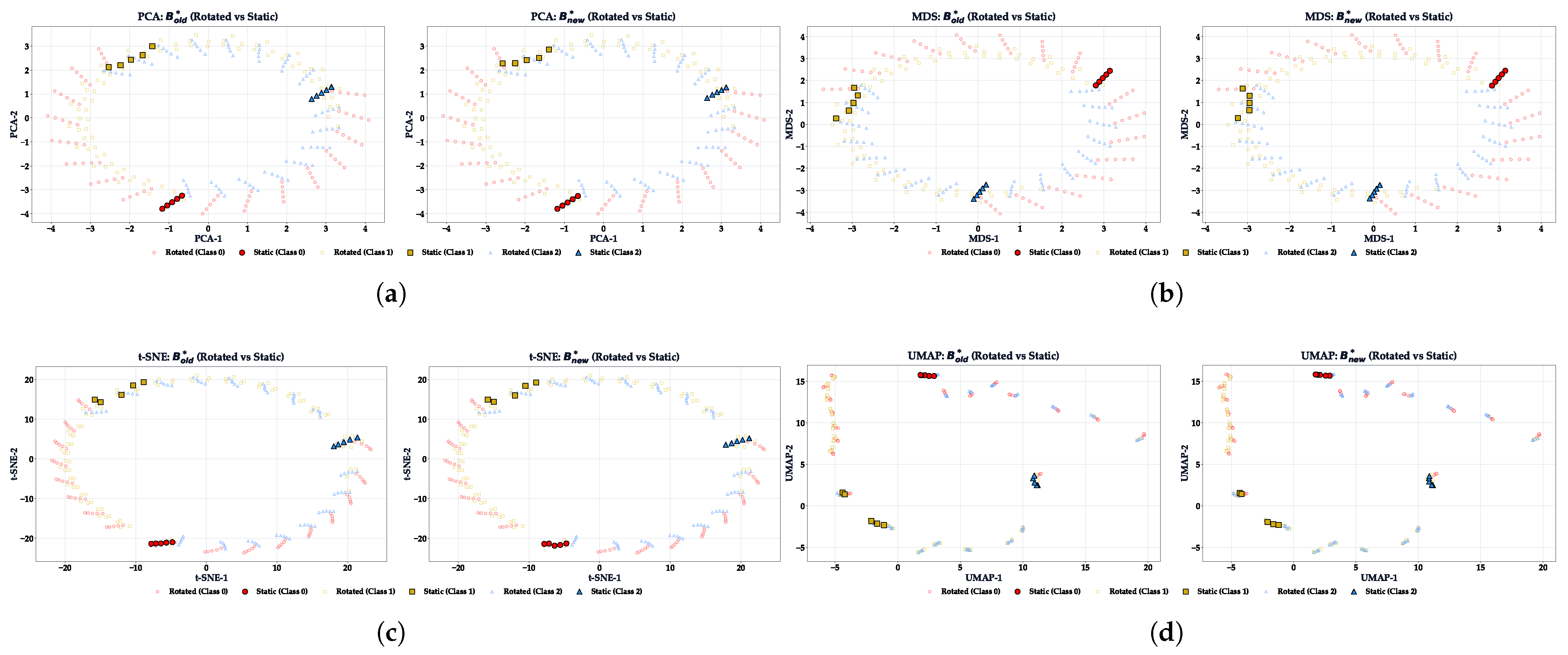
Figure A4.
Singular-value spectrum for the estimation of infinitesimal generators and on the MNIST dataset. The long tails of the spectra (log scale) reveal the presence of near-singular directions, justifying the use of truncated SVD or regularization to obtain stable differential operators for the high-dimensional image and feature spaces.
Appendix D. Additional Reconstruction Visualizations
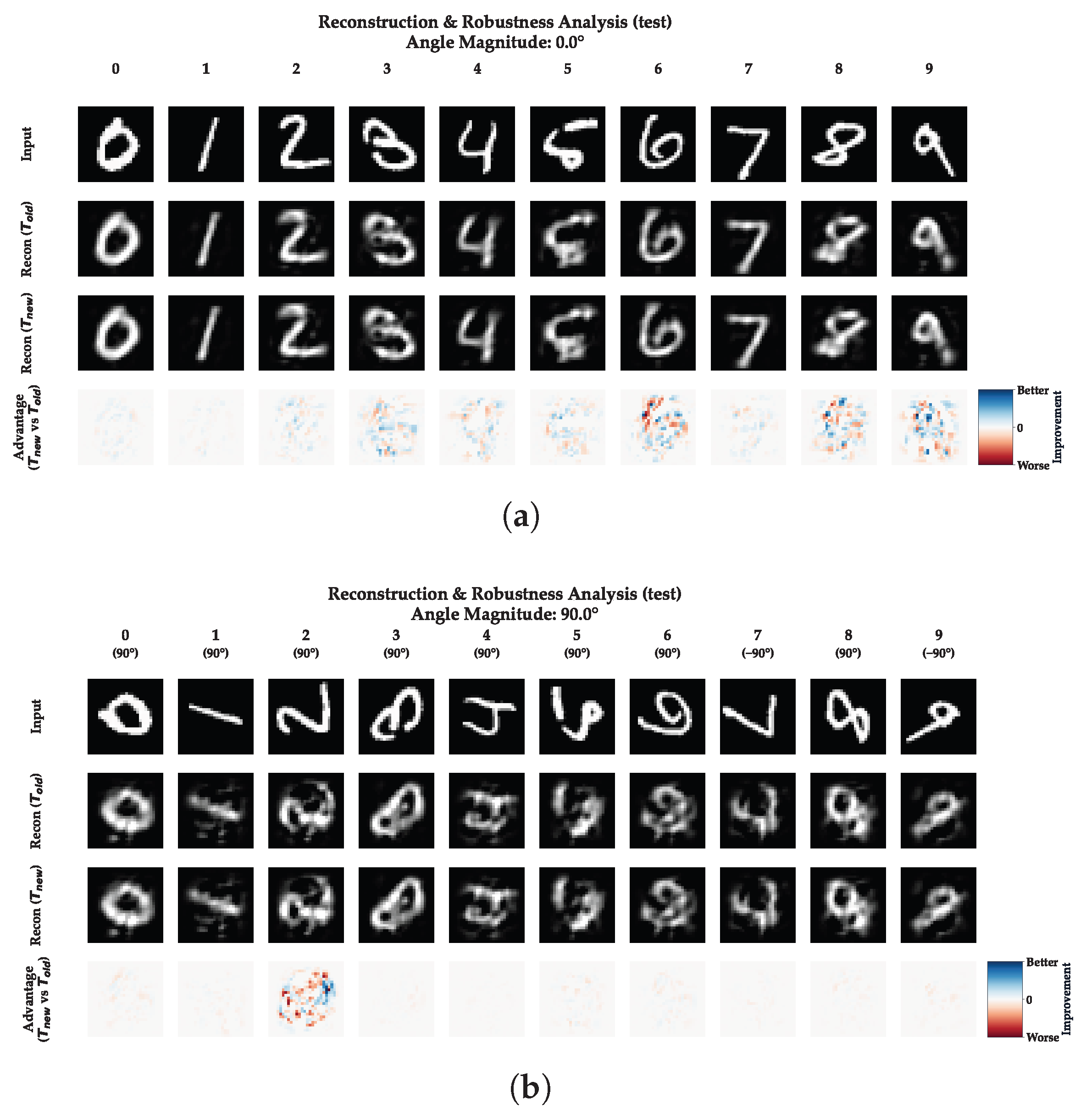
This appendix provides complementary visual comparisons to support the robustness analysis presented in Section 4.2. Figure A5 illustrates the behavior of the ETM versus the baseline at the boundaries of the rotation spectrum.
Figure A5.
Extended qualitative comparison of MNIST reconstructions. (a) At , the ETM approach achieves fidelity comparable to the unconstrained baseline, validating that symmetry regularization does not compromise standard performance. (b) At , ETM exhibits superior structural stability, preventing the geometric distortion observed in the baseline () predictions.
Appendix E. Stability Analysis Visualizations
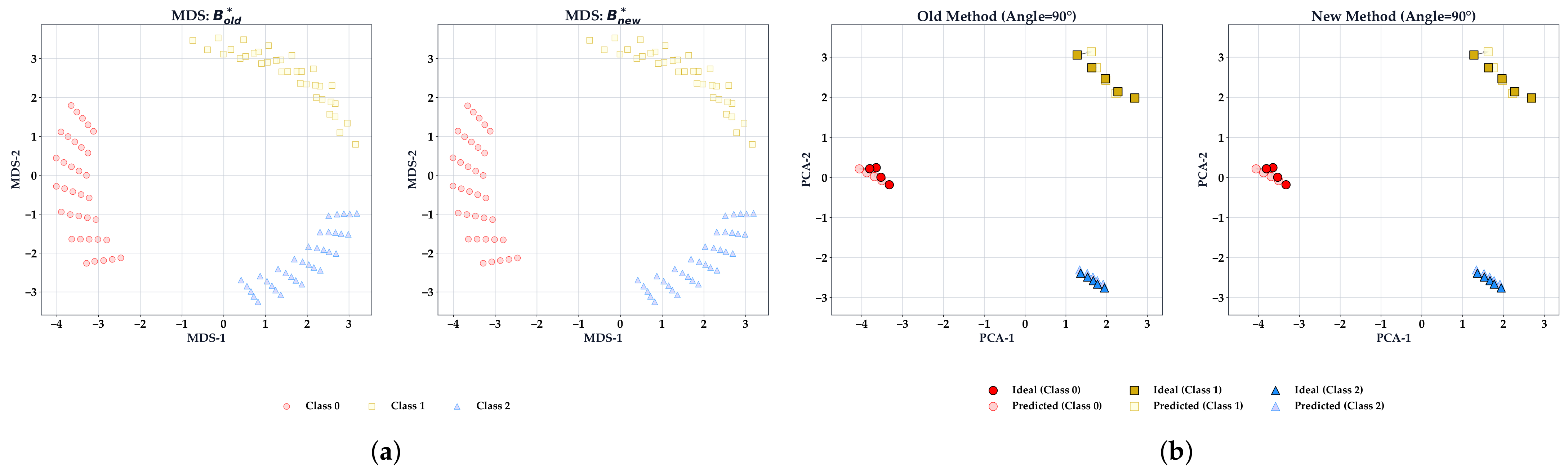
This appendix provides additional visualizations of structural stability analysis under rotation, complementing the MSE vs. angle analysis presented in Figure 6 of the main text.
Figure A6.
Structural stability analysis of the transition mapping under rotation. (a) MDS embedding of sample trajectories in the MM space, comparing the Ideal path, Baseline prediction, and ETM prediction. (b) Displacement vector field illustrating the consistency of transformations between the ideal and predicted representations.
References
- Hassija, V.; Chamola, V.; Mahapatra, A.; Singal, A.; Goel, D.; Huang, K.; Scardapane, S.; Spinelli, I.; Mahmud, M.; Hussain, A. Interpreting black-box models: A review on explainable artificial intelligence. Cogn. Comput. 2024, 16, 45–74. [Google Scholar] [CrossRef] [Scilit]
- Mulder, W.D. Explainable artificial intelligence and the social sciences: A plea for interdisciplinary research. AI Soc. 2025, 40, 2951–2970. [Google Scholar] [CrossRef] [Scilit]
- Andrews, R.W.; Lilly, J.M.; Srivastava, D.; Feigh, K.M. The role of shared mental models in human-AI teams: A theoretical review. Theor. Issues Ergon. Sci. 2023, 24, 129–175. [Google Scholar] [CrossRef] [Scilit]
- Ribeiro, M.T.; Singh, S.; Guestrin, C. Why should I trust you?: Explaining the predictions of any classifier. In Proceedings of the 2016 Conference of the North American Chapter of the Association for Computational Linguistics: Demonstrations; DeNero, J., Finlayson, M., Reddy, S., Eds.; Association for Computational Linguistics: San Diego, CA, USA, 2016; pp. 97–101. [Google Scholar] [CrossRef] [Scilit]
- Sundararajan, M.; Taly, A.; Yan, Q. Axiomatic attribution for deep networks. In Proceedings of the 34th International Conference on Machine Learning, Sydney, Australia, 6–11 August 2017; JMLR.org: Norfolk, MA, USA, 2017; Volume 70, pp. 3319–3328. [Google Scholar]
- Lundberg, S.M.; Lee, S.I. A unified approach to interpreting model predictions. In Proceedings of the Advances in Neural Information Processing Systems; Curran Associates, Inc.: Red Hook, NY, USA, 2017; Volume 30, pp. 4765–4774. [Google Scholar]
- Zhao, X.; Huang, W.; Huang, X.; Robu, V.; Flynn, D. BayLIME: Bayesian local interpretable model-agnostic explanations. In Proceedings of the Thirty-Seventh Conference on Uncertainty in Artificial Intelligence, Virtual, 27–30 July 2021; Curran Associates, Inc.: Red Hook, NY, USA, 2021; Volume 161, pp. 887–896. [Google Scholar]
- Taufiq, M.F.; Blöbaum, P.; Minorics, L. Manifold restricted interventional Shapley values. In Proceedings of the 26th International Conference on Artificial Intelligence and Statistics, Valencia, Spain, 25–27 April 2023; PMLR: Cambridge, MA, USA, 2023; Volume 206, pp. 5079–5106. [Google Scholar]
- Tan, Z.; Tian, Y. Robust explanation for free or at the cost of faithfulness. In Proceedings of the 40th International Conference on Machine Learning, Honolulu, HI, USA, 23–29 July 2023; JMLR.org: Norfolk, MA, USA, 2023; Volume 202, pp. 33534–33562. [Google Scholar]
- Bronstein, M.M.; Bruna, J.; Cohen, T.S.; Veličković, P. Geometric deep learning: Grids, groups, graphs, geodesics, and gauges. arXiv 2021. [Google Scholar] [CrossRef] [Scilit]
- Gerken, J.E.; Aronsson, J.; Carlsson, O.; Linander, H.; Ohlsson, F.; Petersson, C.; Persson, D. Geometric deep learning and equivariant neural networks. Artif. Intell. Rev. 2023, 56, 14605–14662. [Google Scholar] [CrossRef] [Scilit]
- Krak, I.; Kuznetsov, V.; Kondratiuk, S.; Azarova, L.; Barmak, O.; Radiuk, P. Analysis of deep learning methods in adaptation to the small data problem solving. In Lecture Notes in Data Engineering, Computational Intelligence, and Decision Making; Lecture Notes on Data Engineering and Communications Technologies; Babichev, S., Lytvynenko, V., Eds.; Springer: Cham, Switzerland, 2023; Volume 149, pp. 333–352. [Google Scholar] [CrossRef] [Scilit]
- Mehdiyev, N.; Majlatow, M.; Fettke, P. Interpretable and explainable machine learning methods for predictive process monitoring: A systematic literature review. Artif. Intell. Rev. 2025, 58, 378. [Google Scholar] [CrossRef] [Scilit]
- Radiuk, P.; Barmak, O.; Manziuk, E.; Krak, I. Explainable deep learning: A visual analytics approach with transition matrices. Mathematics 2024, 12, 1024. [Google Scholar] [CrossRef] [Scilit]
- Radiuk, P.; Kovalchuk, O.; Slobodzian, V.; Manziuk, E.; Barmak, O.; Krak, I. Human-in-the-loop approach based on MRI and ECG for healthcare diagnosis. In Proceedings of the 5th International Conference on Informatics & Data-Driven Medicine (IDDM 2022), Lyon, France, 18–20 November 2022; CEUR-WS.org: Aachen, Germany, 2022; Volume 3302, pp. 9–20. [Google Scholar]
- Barmak, O.; Krak, I.; Yakovlev, S.; Manziuk, E.; Radiuk, P.; Kuznetsov, V. Toward explainable deep learning in healthcare through transition matrix and user-friendly features. Front. Artif. Intell. 2024, 7, 1482141. [Google Scholar] [CrossRef] [Scilit]
- Kalyta, O.; Barmak, O.; Radiuk, P.; Krak, I. Facial emotion recognition for photo and video surveillance based on machine learning and visual analytics. Appl. Sci. 2023, 13, 9890. [Google Scholar] [CrossRef] [Scilit]
- Cohen, T.; Welling, M. Group equivariant convolutional networks. In Proceedings of the 33rd International Conference on Machine Learning, New York, NY, USA, 20–22 June 2016; JMLR.org: Norfolk, MA, USA, 2016; Volume 48, pp. 2990–2999. [Google Scholar]
- Finzi, M.; Stanton, S.; Izmailov, P.; Wilson, A.G. Generalizing convolutional neural networks for equivariance to Lie groups on arbitrary continuous data. In Proceedings of the 37th International Conference on Machine Learning, Virtual, 13–18 July 2020; JMLR.org: Norfolk, MA, USA, 2020; Volume 119, pp. 3165–3176. [Google Scholar]
- Kondor, R. The principles behind equivariant neural networks for physics and chemistry. Proc. Natl. Acad. Sci. USA 2025, 122, e2415656122. [Google Scholar] [CrossRef] [Scilit]
- Hoffman, J.; Roberts, D.A.; Yaida, S. Robust learning with Jacobian regularization. arXiv 2019. [Google Scholar] [CrossRef] [Scilit]
- Anil, C.; Lucas, J.; Grosse, R. Sorting out Lipschitz function approximation. In Proceedings of the 36th International Conference on Machine Learning, Long Beach, CA, USA, 9–15 June 2019; PMLR: Cambridge, MA, USA, 2019; Volume 97, pp. 291–301. [Google Scholar]
- Lakkaraju, H.; Arsov, N.; Bastani, O. Robust and stable black box explanations. In Proceedings of the 37th International Conference on Machine Learning, Virtual, 13–18 July 2020; JMLR.org: Norfolk, MA, USA, 2020; Volume 119, pp. 5628–5638. [Google Scholar]
- Paige, C.C.; Saunders, M.A. LSQR: An algorithm for sparse linear equations and sparse least squares. ACM Trans. Math. Softw. 1982, 8, 43–71. [Google Scholar] [CrossRef] [Scilit]
- Zhang, L.P.; Li, Z.C.; Wei, Y.; Huang, H.T. New regularization techniques for ill-conditioning problems and their applications: Choices of regularization parameters. Eng. Anal. Bound. Elem. 2023, 152, 347–361. [Google Scholar] [CrossRef] [Scilit]
- Deng, L. The MNIST database of handwritten digit images for machine learning research: Best of the web. IEEE Signal Process. Mag. 2012, 29, 141–142. [Google Scholar] [CrossRef] [Scilit]
- Koh, P.W.; Nguyen, T.; Tang, Y.S.; Mussmann, S.; Pierson, E.; Kim, B.; Liang, P. Concept bottleneck models. In Proceedings of the 37th International Conference on Machine Learning, Virtual, 13–18 July 2020; JMLR.org: Norfolk, MA, USA, 2020; Volume 119, pp. 5338–5348. [Google Scholar]
- Zarlenga, M.E.; Barbiero, P.; Ciravegna, G.; Marra, G.; Giannini, F.; Diligenti, M.; Shams, Z.; Precioso, F.; Melacci, S.; Weller, A.; et al. Concept embedding models: Beyond the accuracy-explainability trade-off. In Proceedings of the Advances in Neural Information Processing Systems; Curran Associates, Inc.: Red Hook, NY, USA, 2022; Volume 35, pp. 21400–21413. [Google Scholar]
- Han, J.; Cen, J.; Wu, L.; Li, Z.; Kong, X.; Jiao, R.; Yu, Z.; Xu, T.; Wu, F.; Wang, Z.; et al. A survey of geometric graph neural networks: Data structures, models, and applications. Front. Comput. Sci. 2025, 19, 1911375. [Google Scholar] [CrossRef] [Scilit]
- Kim, C.; Zhao, S.; Zhu, M.; Lin, T.Y.; Ghaffari, M. Equivariant neural networks for general linear symmetries on Lie algebras. arXiv 2025. [Google Scholar] [CrossRef] [Scilit]
- Battiloro, C.; Karaismailoğlu, E.; Tec, M.; Dasoulas, G.; Audirac, M.; Dominici, F. E(n) equivariant topological neural networks. arXiv 2024. [Google Scholar] [CrossRef] [Scilit]
- Ghorbel, E.; Ghorbel, A.; Ghorbel, F. Equivariant and SE(2)-invariant neural network leveraging Fourier-based descriptors for 2D image classification. In Proceedings of the 17th International Conference on Agents and Artificial Intelligence—Volume 2: ICAART; INSTICC; SciTePress: Setúbal, Portugal, 2025; pp. 210–215. [Google Scholar] [CrossRef] [Scilit]
- Navon, A.; Shamsian, A.; Achituve, I.; Fetaya, E.; Chechik, G.; Maron, H. Equivariant architectures for learning in deep weight spaces. In Proceedings of the 40th International Conference on Machine Learning, Honolulu, HI, USA, 23–29 July 2023; JMLR.org: Norfolk, MA, USA, 2023; Volume 202, pp. 25790–25816. [Google Scholar]
- Pacini, M.; Santin, G.; Lepri, B.; Trivedi, S. On universality classes of equivariant networks. arXiv 2025. [Google Scholar] [CrossRef] [Scilit]
- Crocioni, G.; Bodor, D.L.; Baakman, C.; Parizi, F.M.; Rademaker, D.T.; Ramakrishnan, G.; van der Burg, S.A.; Marzella, D.F.; Teixeira, J.M.C.; Xue, L.C. DeepRank2: Mining 3D protein structures with geometric deep learning. J. Open Source Softw. 2024, 9, 5983. [Google Scholar] [CrossRef] [Scilit]
- Vrček, L.; Bresson, X.; Laurent, T.; Schmitz, M.; Kawaguchi, K.; Šikić, M. Geometric deep learning framework for de novo genome assembly. Genome Res. 2025, 35, 839–849. [Google Scholar] [CrossRef] [Scilit]
- Yim, J.; Trippe, B.L.; Bortoli, V.D.; Mathieu, E.; Doucet, A.; Barzilay, R.; Jaakkola, T. SE(3) diffusion model with application to protein backbone generation. In Proceedings of the 40th International Conference on Machine Learning, Honolulu, HI, USA, 23–29 July 2023; JMLR.org: Norfolk, MA, USA, 2023; Volume 202, pp. 40001–40039. [Google Scholar]
- Alamdari, S.; Thakkar, N.; van den Berg, R.; Tenenholtz, N.; Strome, R.; Moses, A.M.; Lu, A.; Fusi, N.; Amini, A.P.; Yang, K.K. Protein generation with evolutionary diffusion: Sequence is all you need. bioRxiv 2024. [Google Scholar] [CrossRef] [Scilit]
- Martinkus, K.; Ludwiczak, J.; Liang, W.C.; Lafrance-Vanasse, J.; Hötzel, I.; Rajpal, A.; Wu, Y.; Cho, K.; Bonneau, R.; Gligorijevic, V.; et al. AbDiffuser: Full-atom generation of in-vitro functioning antibodies. In Proceedings of the Advances in Neural Information Processing Systems; Oh, A., Naumann, T., Globerson, A., Saenko, K., Hardt, M., Levine, S., Eds.; Curran Associates, Inc.: Red Hook, NY, USA, 2023; Volume 36, pp. 40837–40871. [Google Scholar]
- Krishna, R.; Wang, J.; Ahern, W.; Sturmfels, P.; Venkatesh, P.; Kalvet, I.; Lee, G.R.; Morey-Burrows, F.S.; Anishchenko, I.; Humphreys, I.R.; et al. Generalized biomolecular modeling and design with RoseTTAFold All-Atom. Science 2024, 384, eadl2528. [Google Scholar] [CrossRef] [Scilit]
- Yim, J.; Stärk, H.; Corso, G.; Jing, B.; Barzilay, R.; Jaakkola, T.S. Diffusion models in protein structure and docking. WIREs Comput. Mol. Sci. 2024, 14, e1711. [Google Scholar] [CrossRef] [Scilit]
- Tang, Z.; Li, H.; Lin, P.; Gong, X.; Jin, G.; He, L.; Jiang, H.; Ren, X.; Duan, W.; Xu, Y. A deep equivariant neural network approach for efficient hybrid density functional calculations. Nat. Commun. 2024, 15, 8690. [Google Scholar] [CrossRef] [Scilit]
- Cruz, S.S.; Kolosova, M.; Álvarez, C.R.; Petrucciani, G.; Vischia, P. Equivariant neural networks for robust CP observables. Phys. Rev. D 2024, 110, 096023. [Google Scholar] [CrossRef] [Scilit]
- Wang, C.; Wu, M.; Lam, S.K.; Ning, X.; Yu, S.; Wang, R.; Li, W.; Srikanthan, T. GPSFormer: A global perception and local structure fitting-based transformer for point cloud understanding. In Proceedings of the Computer Vision – ECCV 2024; Lecture Notes in Computer Science; Leonardis, A., Ricci, E., Roth, S., Russakovsky, O., Sattler, T., Varol, G., Eds.; Springer: Cham, Switzerland, 2025; Volume 15066, pp. 75–92. [Google Scholar] [CrossRef] [Scilit]
- Wang, C.; He, S.; Fang, X.; Han, J.; Liu, Z.; Ning, X.; Li, W.; Tiwari, P. Point clouds meets physics: Dynamic acoustic field fitting network for point cloud understanding. In Proceedings of the IEEE/CVF Conference on Computer Vision and Pattern Recognition (CVPR), Nashville, TN, USA, 11–15 June 2025; IEEE: New York, NY, USA, 2025; pp. 22182–22192. [Google Scholar]
- Pearson, K. On lines and planes of closest fit to systems of points in space. Lond. Edinb. Dublin Philos. Mag. J. Sci. 1901, 2, 559–572. [Google Scholar] [CrossRef] [Scilit]
- Kruskal, J.B. Multidimensional scaling by optimizing goodness of fit to a nonmetric hypothesis. Psychometrika 1964, 29, 1–27. [Google Scholar] [CrossRef] [Scilit]
- Hinton, G.E.; Roweis, S.T. Stochastic neighbor embedding. In Proceedings of the Advances in Neural Information Processing Systems; MIT Press: Cambridge, MA, USA, 2002; Volume 15, pp. 833–840. [Google Scholar]
- McInnes, L.; Healy, J.; Saul, N.; Großberger, L. UMAP: Uniform manifold approximation and projection. J. Open Source Softw. 2018, 3, 861. [Google Scholar] [CrossRef] [Scilit]

Disclaimer/Publisher’s Note: The statements, opinions and data contained in all publications are solely those of the individual author(s) and contributor(s) and not of MDPI and/or the editor(s). MDPI and/or the editor(s) disclaim responsibility for any injury to people or property resulting from any ideas, methods, instructions or products referred to in the content. |
© 2026 by the authors. Licensee MDPI, Basel, Switzerland. This article is an open access article distributed under the terms and conditions of the Creative Commons Attribution (CC BY) license.