


Abstract
Generative models hold great potential but only if one can trust the evaluation of the data they generate. It is common to visualize and evaluate quality on two-dimensional visualizations of high-dimensional data. We show that many commonly used quality scores for comparing two-dimensional distributions of synthetic vs. ground-truth data give better results than they should, a phenomenon we call the “grade inflation problem”. We show that the correlation score, Jaccard score, earth-mover’s score, Kullback–Leibler (relative-entropy) score, Jensen–Shannon Score, and Cauchy–Schwarz score all suffer grade inflation to various extents and in various contexts. We suggest that any score that values all datapoints equally, as these do, will also exhibit grade inflation; we refer to such scores as “equipoint” scores. We introduce the concept of “equidensity” scores and present the Eden score as what is, to our knowledge, the first example of such a score. We find that Eden avoids grade inflation and show the highest consistency with human perception of goodness-of-fit of KDEs compared to the equipoint scores above. We propose that any reasonable equidensity score will avoid grade inflation. We identify a connection between equidensity scores and Rényi entropy of negative order. We conclude that equidensity scores are likely to outperform equipoint scores for generative models and for comparing low-dimensional distributions more generally.
1. Introduction
The ability to compare pairs of two-dimensional distributions robustly and accurately is critical in machine learning and in data analysis more generally. This ability is especially valuable in the context of generative models [1] to measure model quality by assessing how well synthetic data fit training data. For example, generative modeling of tabular data, where each row is a datapoint and each column is a feature, has important uses across many fields [2,3,4,5]. Generative modeling is of great interest for imaging and multi-modal data as well [1,6,7]. Although datasets for the latter applications are generally high-dimensional, two-dimensional analysis plays a critical role in quality assessment, either for testing the fidelity of pairwise relationships or via ubiquitous dimensionality reduction techniques such as PCA, tSNE, or UMAP [8,9,10].
Despite its ubiquity, the task of comparing two-dimensional distributions is non-trivial and has led to much work in developing quality scores. At a high level, quality scores can be classified as statistical vs. functional. Statistical scores are designed to demonstrate that some statistic, for example, the mean of one of the features, has the same value in the synthetic dataset as in the real dataset (up to sampling error). In contrast, functional scores are meant to show that the outcome of some procedure, for example, inference, is indistinguishable regardless of whether the input data are real or synthetic (again, up to sampling error) [11]. Statistical scores have the advantage of being easier to calculate and of being generalizable from dataset to dataset; functional scores often take more human and/or compute time and are more likely to be idiosyncratic to a particular dataset. For these reasons, statistical scores have long been, and remain, of general interest.
Statistical scores appear often in the literature on generative modeling, especially of synthetic tabular data. For example, perhaps the two most widely used and easy-to-compute statistics are the correlation coefficient (R) and its square, the coefficient of determination (), which measure the joint distribution between pairs of features (e.g., columns in tabular data). In turn, two common types of correlation coefficient are Pearson’s, which measures linear relationships, and Spearman’s, which is a generalization for any monotonic relationship. For a given pair of columns, one can calculate Pearson’s or Spearman’s R for the real data (), do the same for the synthetic data (), and use them to calculate a correlation score, for example, as [12] or (Division normalizes the range to 0-to-1; subtraction converts the difference into a similarity score). These two versions correlate closely with each other; the first is used more often in the literature, where it is also known as the correlation similarity.
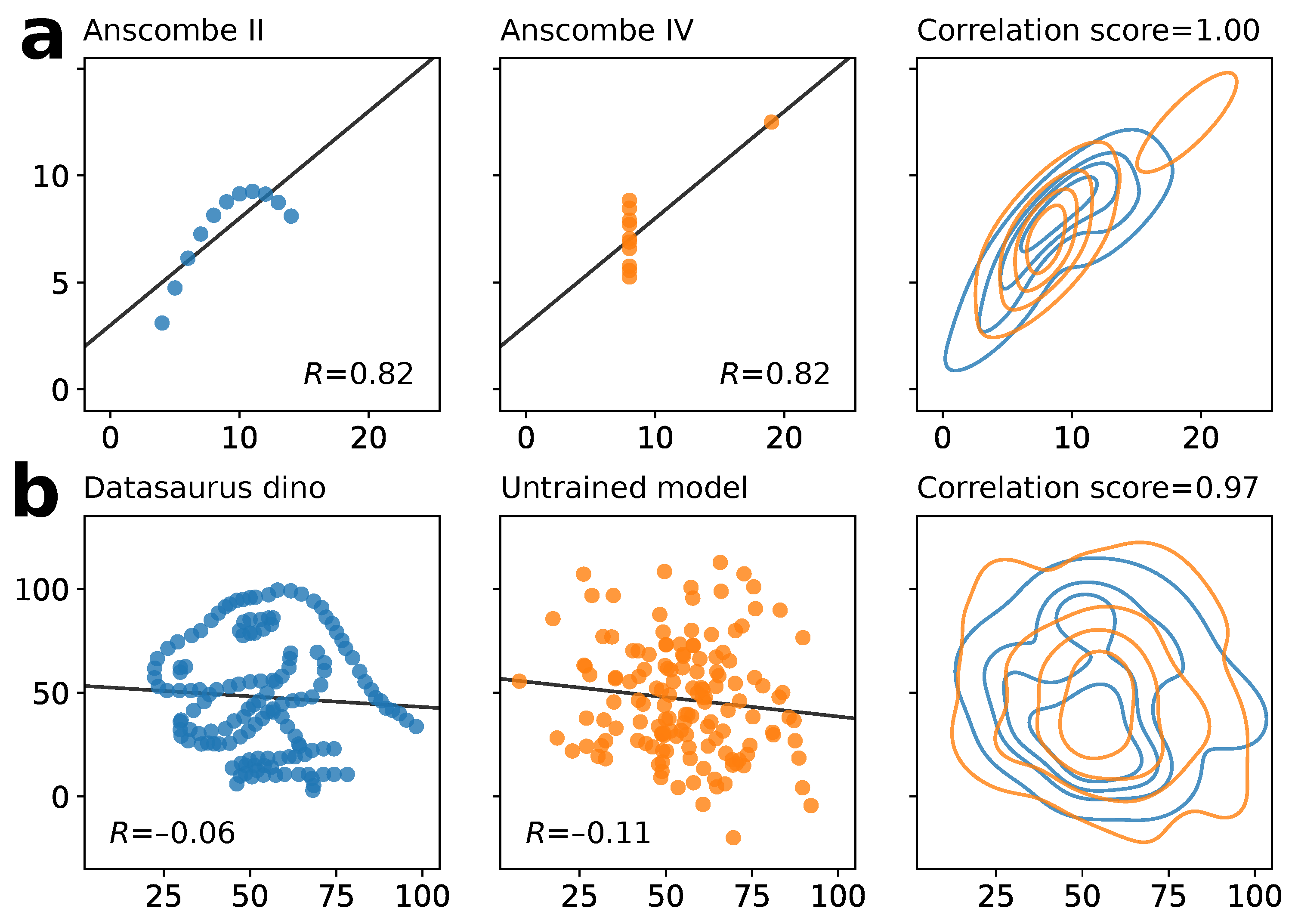
However, there are two important challenges to using the correlation score as a measure of fit between a pair of two-dimensional distributions. The first is the well-known problem that many different distributions can have the same correlation coefficient, as illustrated by examples such as Anscombe’s quartet [13,14] (Figure 1a). Second, there are many more ways to obtain a low correlation than a high correlation. These two challenges can have the following effect. Suppose two columns in the real/training data have some non-random relationship that happens to have a near-zero correlation, for example, like columns in the Datasaurus Dozen datasets [14], and that the synthetic/generated data fail to learn this relationship, resulting in a random distribution (Figure 1b). Because random data have zero correlation (up to sampling variance), the correlation score between the real and synthetic data will be high, despite the low quality of the synthetic data. In principle, such issues can lead to inappropriately high quality scores, a “grade inflation” problem that can make a generative model look better than it is.
Figure 1.
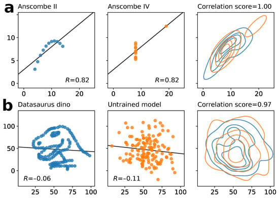
The grade inflation problem. (a) Two distributions from Anscombe’s quartet [13]. Both have a Pearson’s R of 0.82, meaning their correlation score is 1.00 despite their differences (which are appreciable in their KDEs, right, which are color-coded to match the distributions). Black lines show least-squares regression fits to illustrate indistinguishable slopes and intercepts. (b) A highly non-random distribution from the Datasaurus Dozen [14] and (Gaussian-distributed) synthetic data with the same means and standard deviations from an untrained generative model. Pearson’s R of −0.06 and −0.11, respectively, resulting in the very high correlation score of 0.97 despite the poor fit.
To further characterize the grade inflation problem, here, we evaluate several additional quality scores: the earth-mover’s score (also known as earth-mover’s, Mallow, Wasserstein, or Kantorovich–Rubenstein distance), Jaccard score, Kullback–Leibler (KL) divergence (also known as the relative Shannon entropy), the Jensen–Shannon (JS) divergence (a symmetric/balanced form of KL), and the Cauchy–Schwarz (CS) divergence. We find that many of the more commonly used measures can fall prey to grade inflation. To address this problem, we introduce and describe a new score, the Eden score, that appears to avoid grade inflation. Our investigation focuses on two-dimensional distributions and pairwise relationships, which are often effective—sometimes “unreasonably” so [15,16]—at capturing key relationships in high-dimensional data.
The main contributions of this paper are as follows:
- Identification of the grade inflation problem afflicting many of the most commonly used statistics in the evaluation of generative models.
- Introduction of the Eden score as a measure that is highly consistent with human expert judgment and appears to avoid grade inflation.
- Benchmarking of seven measures to evaluate goodness of fit of synthetic data against human visual inspection.
- Repeat sampling is necessary to avoid misleading results.
2. Methods
2.1. Datasets
We generated synthetic data from both in-house two-dimensional toy datasets (called Dart, Trimodal, and Stripes) and the following high-dimensional machine-learning datasets obtained from the University of California Irvine machine learning repository (UCIMLR): Covertype, Communities and Crime, Energy Efficiency, and Rice (Cammeo and Osmancik) (UCIML ID nos. 31, 183, 242, and 545, respectively). The latter were retrieved using the lucie Python package [4]. Anscombe’s Quartet was obtained via the seaborn Python package. The Datasaurus Dozen were obtained via https://www.autodesk.com/content/dam/autodesk/www/autodesk-reasearch/Publications/pdf/SameStatsCode.zip (accessed 15 October 2026) from the file DatasaurusDozen.tsv.
2.2. Generative Models and KDEs
The following models/model architectures were used to generate synthetic data: an in-house implementation of Gaussian Copula [17], CTGAN as implemented in the SDV package [12,18,19], a flow-based model from the Python package nflow [20], as well as in-house energy-based models [21]. KDEs were generated using the gaussian_kde function of Python’s scipy package with levels = 5 but otherwise default parameters [22]. Note in gaussian_kde, the bandwidth of the KDEs is given by Scott’s method [23], and the lowest 5% of the probability mass is ignored when finding the likelihoods of the contours.
2.3. Scores Used
We consider seven different quality scores. The correlation, earth-mover’s, and Jaccard scores and the KL [24], JS, and CS divergences are based on prior work referenced below; the Eden score is newly described in this work (see below).
2.3.1. Correlation Score
The correlation score is defined using Pearson’s R as . Here and throughout this section, p and q the two distributions or samples from the two distributions (e.g., real vs. synthetic data). , are the Pearson correlations between the x and y coordinates of the points in distribution p and q, respectively. This definition reflects the most common definition we found in the literature.
2.3.2. Earth-Mover’s Score
The earth-mover’s score [25,26,27,28] is defined as , where denotes the empirical 1-Wasserstein distance from the ot python package [29]. We standardized both real and synthetic data using the mean and standard deviation of the real data prior to computing .
2.3.3. Jaccard Score
The Jaccard score, also known as the Jaccard index and intersection-over-union (IoU) [30,31], is defined as
where the numerator is the size of the intersection between the two distributions p and q, and the denominator is the size of their union [31]. The union is taken to be the total number of samples. Because p and q (as samples), generically speaking, do not contain points in common, we define the intersection as follows for tabular datasets. We fit one Gaussian KDE model to the real data and a second Gaussian KDE to the synthetic data to define the intersection. We denote these real and synthetic KDEs and , respectively. We take the intersection to be
Thus, a point in the real data is in the intersection if its likelihood as evaluated by the synthetic KDE is sufficiently close to the maximum likelihood of the synthetic KDE (with “sufficiently close” defined as the ratio of the two likelihoods ), and similarly for the synthetic data. We note that due to this subtlety with defining the intersection, our Jaccard score is a modified version of the standard Jaccard score.
2.3.4. Kullback–Leibler Score
The KL divergence is a special case of the Rényi divergence between two continuous distributions, defined as
is called the order parameter; the KL divergence is the Rényi divergence in the limit of . We defined the KL score as the exponential of the negative KL divergence:
with p and q as above, approximated using Gaussian KDE also as above. Since the KL divergence takes values between 0 and ∞, the KL score has the desirable range . We approximated the integral for by the Monte-Carlo method, which introduces (minor) stochasticity into the KL score. The Monte-Carlo approximation is as follows. We have
which can be rewritten as an expectation value:
which, in turn, can be estimated from a sample of p:
where N is the sample size.
2.3.5. Jensen–Shannon Divergence (JS)
JS is a symmetric and bounded measure derived from the KL divergence [32]. Unlike KL divergence, JS remains finite when the two distributions have non-overlapping support and treats the two distributions symmetrically.
JS is defined as
where p and q denote the probability distributions of the real and synthetic data, respectively, and M is the mixture distribution
To keep measures comparable, we find the probability distribution for the real and synthetic the same way as in the calculation of KL (mentioned above). We then used Monte-Carlo to estimate the integral and took exponential of the negative JS to have a similarity score
2.3.6. Cauchy–Schwarz Divergence (CSD)
CSD quantifies the difference between two probability distributions based on the overlap between their probability density functions [33]. For two continuous probability density functions, p and q, the CSD is defined as
Integrals here were calculated with gaussian_kde from the package. A value of zero indicates identical estimated distributions, while larger values indicate decreasing overlap between the distributions. Calculated CSD is then converted to a score as follows:
2.3.7. Eden Score
In the Eden score, the difference between two KDEs is calculated by calculating the difference for each successive ring or “annulus” defined by the contours of the KDEs and averaging these differences. For each annulus in the real/synthetic data, we define a per-annulus similarity score. Without loss of generality, we label the outermost annulus 0, the second-outermost annulus 1, and so on. (The unbounded region outside of all contours is excluded). Define the per-annulus score by a variation of the Jaccard formula (Equation (1)), with the area playing the role of size
The Eden score is obtained by averaging scores over all annuli:
Here, is the number of annuli scored. In our Python implementation, the parameter n_of_levels specifies the number of contour levels, so that . Note, technically, the innermost annulus is usually a disk representing the peak of the distribution, and any annulus can consist of non-contiguous densities (e.g., multiple disks/peaks). was used throughout this paper, corresponding to .
To estimate the areas in the numerator and denominator of Equation (11), a Monte-Carlo method is used: a bounding rectangle centered at the data is sprinkled with a large number of uniformly distributed points; the number of points that lie inside the union/intersection of a real and a synthetic annulus i is counted. To determine whether a point lies inside a union/intersection of two annuli, we compute the likelihood of the point under and and check whether the likelihood falls within the likelihood range that defines two adjacent contours. As with the KL score, this process introduces minor stochasticity. In Appendix A, we provide the explicit Python implementation of the Eden score.
2.4. Validation
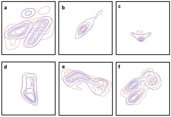
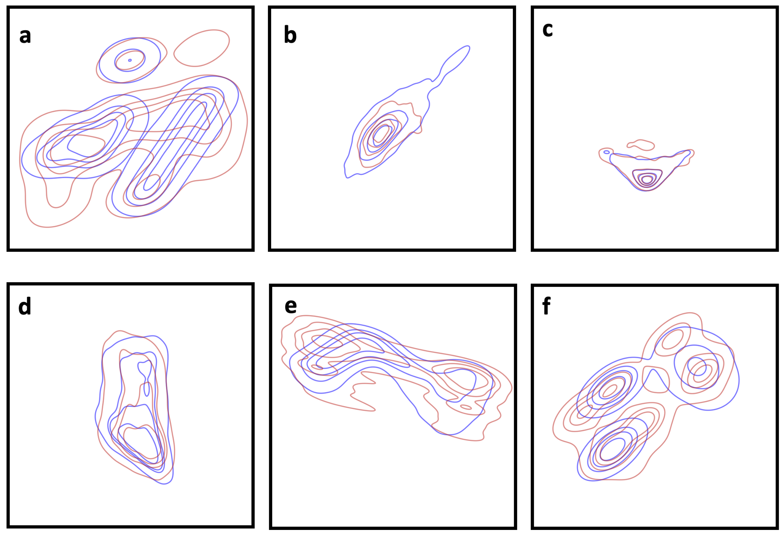
Human visual inspection widely serves as a benchmark qualitative assessment of synthetic data, in many cases, accompanying quantitative methods like different scoring measures. However, this procedure can be expensive in terms of human time, especially when domain expertise is scarce. Having quantitative methods accurately reflecting human judgment can thus be cost-effective in large-scale evaluation settings. We thus used human visual inspection as the baseline for comparison of two-dimensional distributions. Consequently, 39 pairs of plots from 6 datasets were shown to 20 human raters. Raters all had a background in data science, science, and/or engineering to increase the likelihood of exposure to/familiarity with the general practice of data presented as KDEs. Each plot consisted of two superimposed KDEs in different colors, corresponding to training data and synthetic data output by a generative model. Plots were chosen so that Eden score disagreed with at least one of the other scores in higher quality fit among the pair in a statistically significant way. Details of datasets used and score calculation can be found in Table 1 and Figure 2, and code is made available in https://github.com/ArnaoutLab/Grade-Inflation/ (accessed 15 October 2026). Scores were not shared with the human raters, making this a blind test.
Table 1.
Datasets and features used in the experiments.
Figure 2.
Example of plots used in validation experiment from datasets mentioned in Table 1. Raters are shown a pair of plots, each consisting of superimposed KDEs of “real” (training) and synthetic data. Each red-blue pair shares the same real data with which two synthetic model of different qualities were trained.
Each human rater was asked to choose the plot in which the contours matched better, considering all contours; the interpretation of “better” was otherwise left up to the rater. The 39 pairs corresponded to three repeats of each of 13 unique pairs of columns. For each repeat, the pair was subjected to color swaps, and mirroring and the left–right order of the plots were randomized; this allowed for a per-person test of consistency, to assess whether the rater picked the same plot all three times regardless of position, orientation, and color. Whichever unique pair the rater chose for at least two out of three repeats is considered the rater’s preference. Separately (i.e., without the rater), the fit in each plot was scored according to each of the seven scoring methods—correlation, earth-mover’s, Jaccard, KL, JS, CS, and Eden score—to determine the higher-scoring plot in each pair. In cases where the rater chose a winner but the scoring method tied, the scoring method was treated as disagreeing with the rater, since the rater but not the scoring method was able to distinguish between the pair. Cohen’s kappa was used to calculate the agreement between each rater and each scoring method. To test the hypothesis that Eden is more resistant to grade inflation and thus more consistent with human raters, the one-sided Wilcoxon signed-rank test was performed to test the null hypothesis that Eden is not better than each alternative (Python, scipy.stats.wilcoxon). p-values were corrected for multiple comparisons by the Holm method (with n = 6).
3. Results
3.1. Correlation Score
To illustrate how the correlation score can lead to grade inflation, we first measured this score between pairs of distributions from Anscombe’s quartet. The four distributions in this set were devised in 1973 to show how different distributions can have identical Pearson’s R (to several significant digits). Figure 1a illustrates the outcome: a perfect correlation score, despite the two distributions differing materially from each other. This is grade inflation. The “dino” dataset from the Datasaurus Dozen illustrates the compounding problem that arises as a result of low-correlation distributions being more common than high-correlation ones (Figure 1b). Specifically, treating dino as the training set, we randomly initialized a generative model with the same x and y means and standard deviations and sampled from that model without any training. The dino dataset has a Pearson’s R of close to zero. Random data also have a Pearson’s R of close to zero. Because these values are similar, the correlation score is nearly perfect—0.97 in the sample in Figure 1b—despite the model knowing literally nothing beyond the location and scale of the data. Again, this is grade inflation.
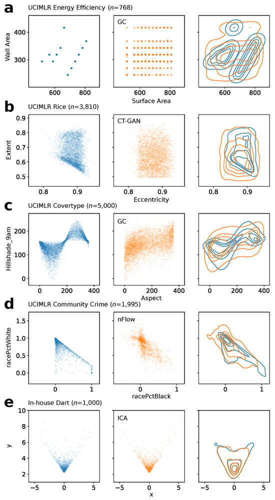
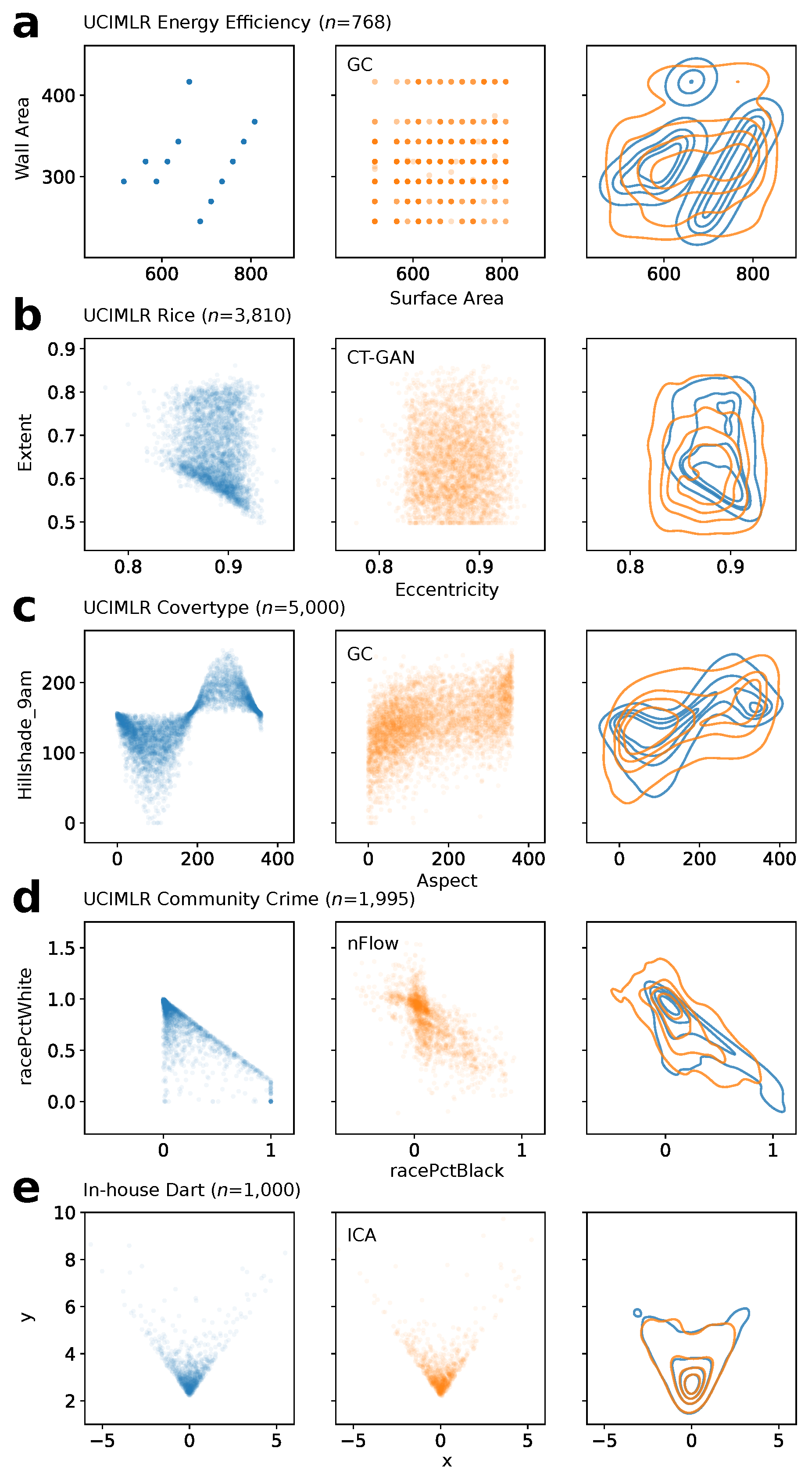
To illustrate the phenomenon on datasets and generative models used in real-world data science, we applied a variety of models to a selection of datasets from the UCIMLR and measured the correlation score between the synthetic/generated data and the real/training data, for representative pairs of columns (Figure 3a–d). Even when fits were low quality by eye, the correlation score was universally high, ranging from 0.903 to 0.994 (Table 2), demonstrating grade inflation. As a positive control, we also scored a high-quality model fit of an in-house dataset called Dart (Figure 3e). Not surprisingly, the correlation score was also excellent, at 0.981, but notably, this score was actually lower than the 0.994 achieved by the low-quality fit in Figure 3a (Table 2). Thus, the correlation score has difficulty differentiating between high- and low-quality fits, leading to grade inflation for some of the latter.
Figure 3.
Fits scored in Table 2. Left to right: real data (blue), generated synthetic data (yellow), and KDEs. (a) is considered a very low-quality fit; (b–d) are considered low-quality fits; (e) is considered a high-quality fit. Datasets, sizes, features, and models are as labeled. UCIMLR = UC Irvine Machine-Learning Repository. GC = Gaussian copula. nFlow = normalizing flow. ICA = independent component analysis.
Table 2.
Scores for the fits and samples in Figure 3. Figure 3a–d are considered very low- or low-quality fits deserving lower scores; Figure 3e is considered a high-quality fit deserving higher scores. Results for Eden in bold. See Section 3 for details. Standard deviations are reported for scores whose calculation involves a stochastic element (Section 2); they are not for repeat sampling (see Section 3.9).
3.2. Earth-Mover’s Score
The earth-mover’s distance (EMD) is more sophisticated and is the basis of the Frechet inception distance, which is commonly used in machine learning [34]. If each two-dimensional distribution is a pile of sand, the EMD is the minimum amount of work required to transform one distribution into the other by moving sand around. EMD is easily converted to a score with range via exponentiation. To apply the resulting earth-mover’s score, the finite collections of datapoints in each distribution are binned into histograms. (Note, the algorithm used here, from [35], does not require smoothing the data by KDE, though that is an alternative approach). In its native form, the EMD has the undesirable feature of being sensitive to the overall number of data points; to avoid this scale-dependence, the real and synthetic data are generally normalized, as we do here, before computing the score.
We calculated the earth-mover’s score for each fit in Figure 3 and found that even though the overall scale is not as inflated as correlation similarity (scores all above 0.9), the score range from 0.5 to 1 in examined examples, interpreted as inflation for lower quality fits. This means that on the lower end of the score, the earth-mover’s score may lack sufficient granularity to differentiate fit quality. For example, the earth-mover’s score was 0.605 for very poor fit as Figure 3a and considered it a better fit than Figure 3b (which received a worse score, 0.508). One can change the overall scaling of the scores by choosing a different value of k, but this does not resolve the grade inflation in Figure 3a,b, because scaling so that lower quality fits have lower scores has the adverse effect of also reducing the score of high-quality fits. Since changing k does not change the ordering of scores, it cannot thread this needle. It is also noteworthy that the earth-mover’s score can be highly sensitive to outliers, since the optimal transport might be such that the outliers have to be moved over further distances compared to more central points (see Section 4).
3.3. Jaccard Score
A score often used in the evaluation of generative models is the Jaccard score or intersection-over-union (IoU). It has the desirable range of 0 to 1. It does not exhibit the earth-mover’s score’s outsize sensitivity to outliers, since the relative distance between non-intersecting densities does not enter into the equation (Section 2). In our analysis, the Jaccard score was found to behave like the correlation score in that values were similar regardless of whether fits were high- or low-quality (Table 2). The main differences were (1) the range of scores was lower than for the correlation score, and (2) one of the low-quality fits—Figure 3d, with a Jaccard score of 0.644—scored 0.2 lower than the others, which ranged from 0.811 to 0.870. Importantly, the score of 0.834 for the high-quality fit (Figure 3e) was actually lower than for the lowest-quality fit (0.870 for Figure 3a), indicating grade inflation. We found that the Jaccard score is especially prone to grade inflation when one distribution completely circumscribes the other. Together, these results support the conclusion that, like the correlation and earth-mover’s scores, the Jaccard score is not a dependable discriminant of quality in generative models, due to grade inflation.
3.4. Kullback–Leibler Score
A third relevant quality score is based on the KL divergence, also known as relative Shannon entropy. This quantity is interpreted as the information lost, or the “surprise”, in approximating one distribution by another [36,37]. It is used widely in generative models, although in our reading of the literature, not as frequently for evaluating synthetic data as the correlation, earth-mover’s, or Jaccard scores. However, the ubiquity of the KL divergence and its utility comparing two-dimensional distributions make it a natural comparator.
KL divergence is one of a family of Rényi divergences parameterized by , the order. From Equation (3), weights the extent to which the density of p contributes to . For , is almost completely determined by the highest-density region of p. In contrast, for (the most extreme example of negative order), the sign flip results in being almost completely determined by the highest-density region of q; i.e., the roles of p and q are essentially swapped (’s sign is also flipped). Meanwhile, means density is not weighted at all, resulting in the trivial result of for all p and q (assuming p and q do not vanish anywhere): this is because any distributions p and q are trivially indistinguishable if one ignores their density distributions. KL divergence corresponds to . The divergence is easily converted into a score by exponentiation (Section 2).
While the KL scores from Table 2 are not the highest in absolute terms, the fit for Figure 3a suffers grade inflation relative to the fits for Figure 3c,d, which are better fits by eye but have similar scores. The reason for the grade inflation in this case is because the real and synthetic data have similar support but different numbers of modes [37], as follows. Recall that KL divergence can be understood as the amount of surprise at the real data, given the synthetic data. In Figure 3a, the synthetic data have a single mode, with a support that spans the real data’s two main modes. Even though the fit is low quality, it does have density that overlaps the centers of the two main modes in the real data. As a result, the surprise factor at finding density in these regions of the real data is low, inflating the KL score (which varies inversely with the divergence), despite the low-quality fit. This inconsistency is a drawback of the KL score.
3.5. Jensen–Shannon Score
Derived from KL divergence, JS divergence compares distributions in both directions, making it symmetric where KL is not; in addition, the JS divergence always has an upper bound:
As a result, the JS score based on tends to exceed the KL score in magnitude. Moreover, since the JS divergence is based on the mixture distribution (see Section 2) instead of one single distribution, it is thus less sensitive to extreme values and has a smaller variance. We have observed both features when evaluating the examples in Figure 3. Compared to the KL score, the JS score suffers more from grade inflation, with scores ranging from 0.732 to 0.993 for observed examples. For Figure 3b,d, the scores are both close to 0.9 despite obvious visual differences in fit.
3.6. Cauchy–Schwarz Score
Compared to the other measures, Cauchy–Schwarz divergence appears less often in the literature on generative-model evaluation. In general, this measure suffers less from the grade inflation problem and is free from ordering issues in the examples in Figure 3. Since CS divergence can be interpreted as a normalized collision frequency, this equal-point measure scores more reasonably (0.565) in cases where the real data have a relatively small number of unique values and the synthetic data “spreads out” around these values (Figure 3a). However, when distributions become less discrete and cover more area, the CS score also starts to overlook major failures in the fit. Like the other equal-point measures, CS score can be biased by good distribution in the high-density area but ignore violations in low-density areas. For example, in Figure 3d) the CS score was 0.921 though a considerable portion of synthetic data exceeded the [0, 1] range set by the data (which, in this case, was a pair of percentages).
3.7. Eden Score
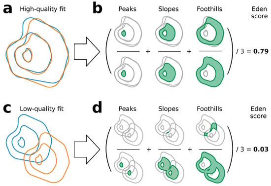
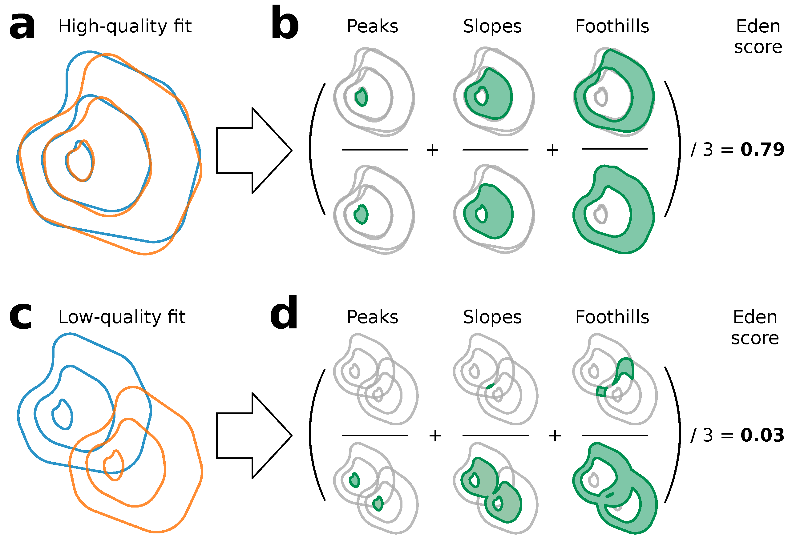
The Eden score differs qualitatively from the others in being an equidensity score, hence its name (see Section 4). Eden is based on the principle that a distribution p is a good match of a distribution q if their regions of probability density i coincide for all densities i. Any reasonable method can be used for determining coincidence; we use the Jaccard score, since Jaccard exhibits grade inflation only when densities vary, which is definitionally not the case for equidensity regions; therefore, unlike when comparing complete distributions, comparison of equidensity regions should not have this problem. To calculate the Eden score, the Jaccard score is calculated for each annulus or ring of density i, and these scores are then averaged (Figure 4). All contours of the distribution count equally, avoiding the issues encountered with the earth-mover’s and Jaccard scores (and, of course, with the correlation score).
Figure 4.
The Eden score. The Eden score comparing the blue and yellow distributions in the high-quality fit in (a) is calculated as the mean intersection-over-union for each equidensity contour (ring, annulus) (b). Peaks, slopes, and foothills contribute equally. Top row of (b), intersections; bottom row, unions (both in green). The ratios for the three contour levels shown are 0.77, 0.81, and 0.78 (left-to-right), which average to an Eden score of 0.79 for the fit of the two distributions in (a). For clarity, the score is calculated over three contours, instead of the five used in the rest of this study. (c,d) Similar for a low-quality fit. The peaks are disjoint (ratio, 0.00), the slopes intersect by only a sliver (ratio, <0.01), and the foothills’ intersection-over-union is 0.09, yielding an Eden score of 0.03.
Indeed, calculation of the Eden score for each of the fits in Figure 3 showed that it avoids grade inflation (Table 2). Scores for the low-quality fits in Figure 3a–d ranged from 0.162 to 0.261 vs. 0.853 for the high-quality fit in Figure 3e. (The confidence intervals in Table 2 account for the stochastic element in our implementation, which can be made arbitrarily small by scaling up the Monte Carlo; the same is true for the KL score. The others are deterministic). Eden was the only score to demonstrate a consistent gap between low- and high-quality fits, without exceptions. Moreover, this gap was sizable, at 3–4-fold. Thus, it was immune to grade inflation in these examples.
3.8. Validation
To validate our results, we showed 39 pairs of KDE plots to each of 20 scientists, data scientists, and engineers. Each plot consisted of contour plots of training data and generated (synthetic) data, plotted on top of each other. The same training data were shown in each plot in the pair; the generated data differed between the two plots in the pair. The human rater was asked to choose which plot represented the better fit. We then calculated Cohen’s to analyze agreement between human raters and each scoring method.
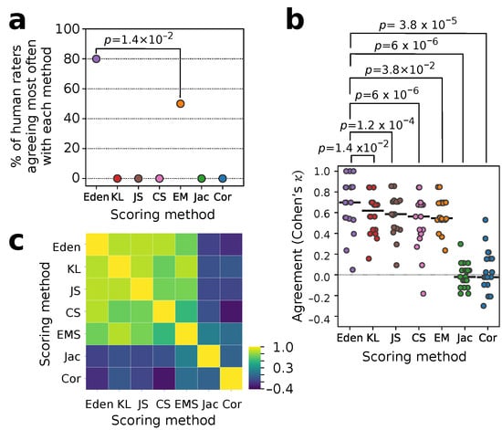
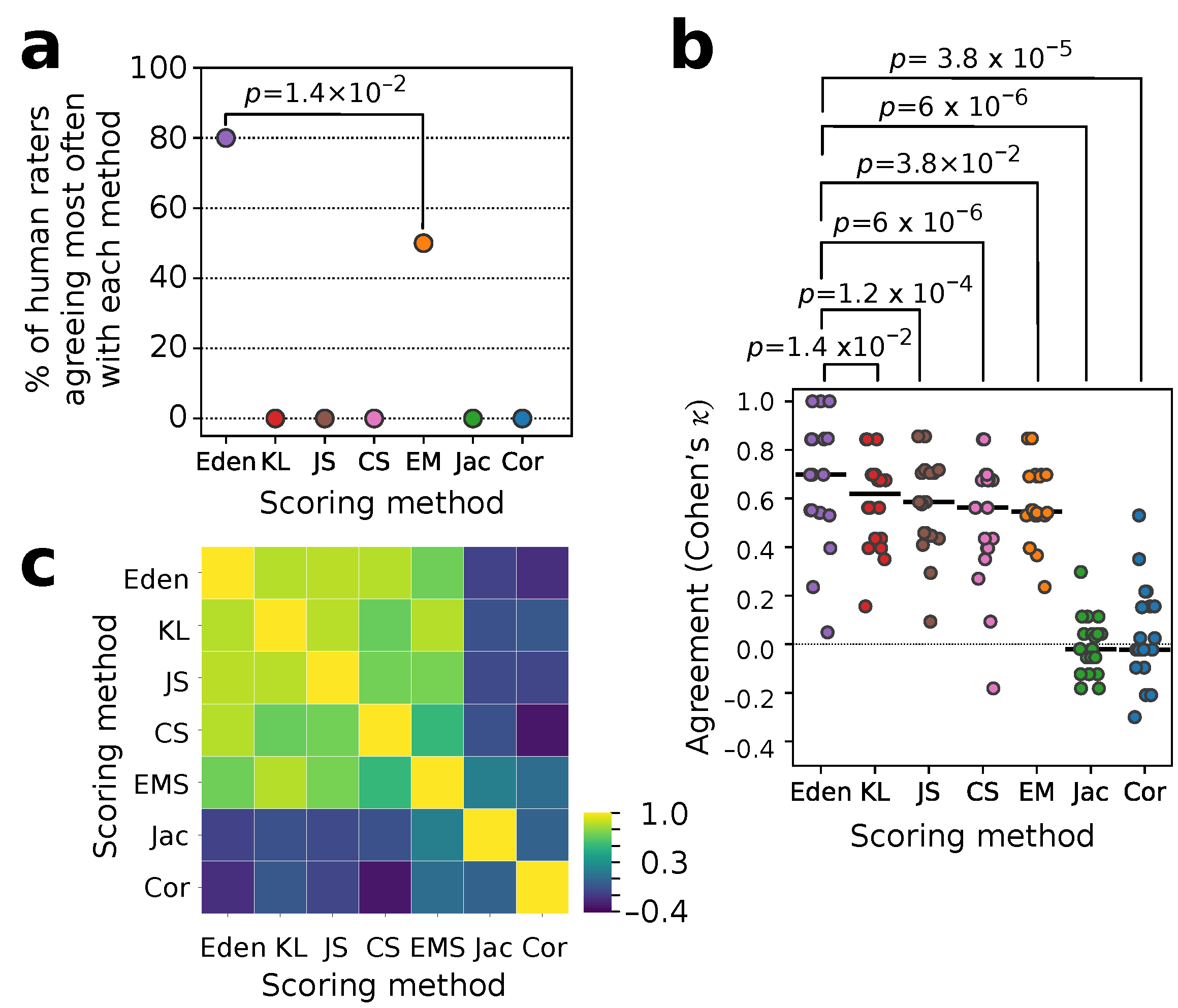
We ranked scores by how often raters agreed with each of them, measuring agreement between each rater and each score using Cohen’s . We found that Eden was the no. 1 choice for 80% of raters (including ties). The earth-mover’s score was the no. 1 for 50% (p-value for difference between ranks, ); no other score was the no. 1 choice (Figure 5a). We also compared the distribution of s between scores, to assess whether preferences were statistically significantly different (Figure 5b). Eden had the highest median agreement at , representing “substantial” [38] agreement. KL had the second-highest at —still “substantial” agreement—but was significantly lower (). The JS, earth-mover’s, and CS scores all exhibited “moderate agreement” with medians of 0.59, 0.56, and 0.55, respectively. The Jaccard and correlation scores were by far the worst, with near-zero median s. Of note, the near-zero median s of the correlation and Jaccard scores indicate that agreement between these scoring methods and humans with domain expertise is no better than chance, arguing against their use. In contrast, Eden’s showed excellent agreement with human raters.
Figure 5.
Validation. Twenty human experts were each asked to rate which of two fits was better for several pairs. Ratings were then compared against each of the five statistical scoring methods. Agreement between each human rater and the scoring method on the unique 13 pairs was measured by Cohen’s . (a) Percent of raters who agreed the most with each scoring method (Eden, KL, etc.). p-value is for Wilcoxon signed-rank test (adjusted for multiple comparisons). (b) All values for each score, with Wilcoxon signed-rank test p-values (also adjusted for multiple comparisons; see Section 2). (c) Agreement between methods for test pairs (again measured by ).
Together with its avoidance of grade inflation, including both its clear segregation between low- and high-quality fits and its scoring consistency, Eden’s performance supports its use for evaluating two-dimensional distributions.
3.9. Confidence Intervals
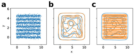
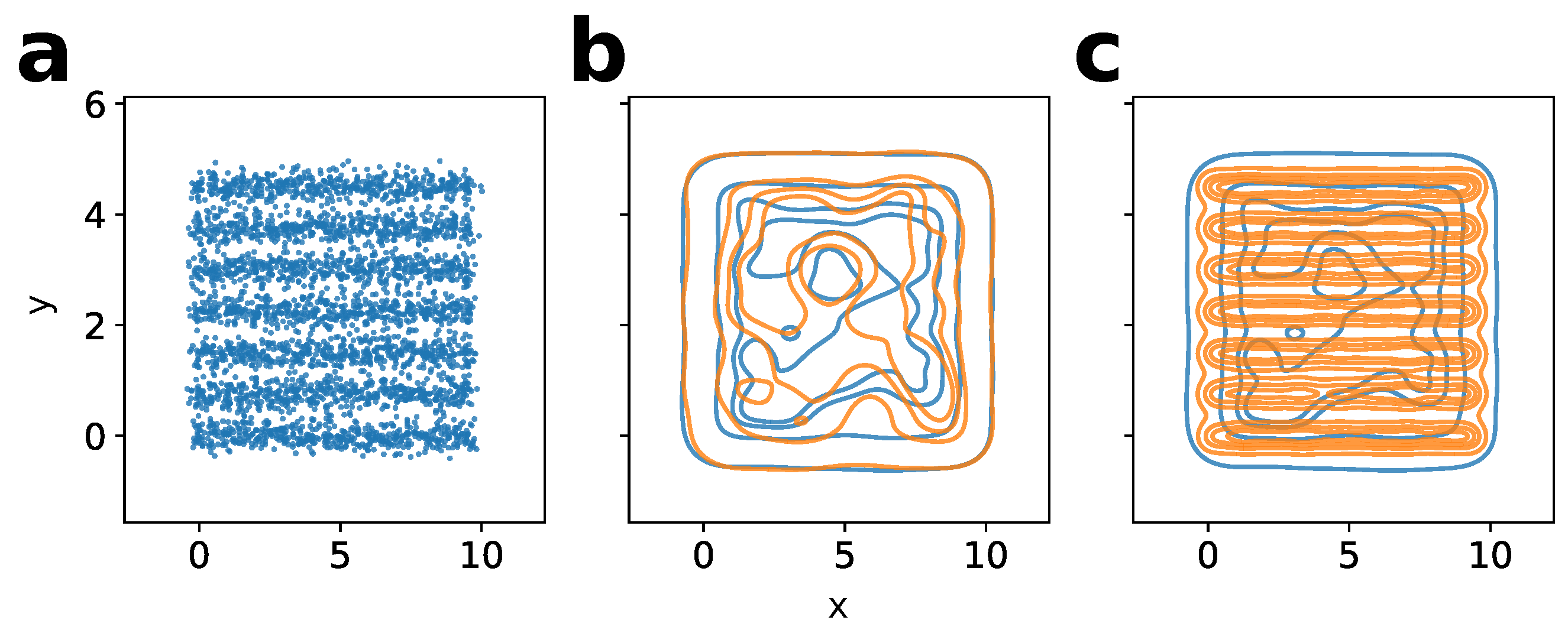
For the most direct, apples-to-apples comparisons, generated synthetic data should have the same number of datapoints as the training data. However, synthetic data are often needed precisely because the training dataset is small; in principle, sampling the equivalent small number of synthetic datapoints can result in comparatively large sampling error in quality scores. Nevertheless, we found that the alternative of oversampling from the model can result in a synthetic-data KDE that is qualitatively sharper than that of the real dataset, potentially complicating comparisons (Figure 6). To illustrate, we trained a Gaussian copula on a target with a striped pattern (Figure 6a). The normal KDE plot (i.e., without oversampling of the synthetic data) does not pick up the stripes (Figure 6b), whereas the KDE plot with oversampled synthetic data does (Figure 6c). This lowers the Eden score (from 0.430 to 0.177), as might be expected from how different the KDE becomes. Of the seven scoring methods, Eden, KL, JS, and CS were sensitive enough to noticeably fall in response to this difference. The Jaccard score fell by just 0.001; the correlation and earth-mover’s scores actually rose. Note that all the scores other than Eden were all ≥0.948 to begin with, reflecting the grade inflation problem.
Figure 6.
Oversampling affects scoring. (a) Target (in-house “Stripes” dataset). (b) Sample (orange) the same size as the target. Correlation, earth-mover’s, Jaccard, KL, JS, CS, and Eden scores: 0.988, 0.948, 1.000, 0.998, 0.998, 0.999, and 0.430, respectively. (c) Oversampling. Scores (same order): 0.999, 0.968, 0.999, 0.899, 0.982, 0.973, and 0.177. Eden is the most sensitive to the difference in KDEs between normal sampling (b) and oversampling (c).
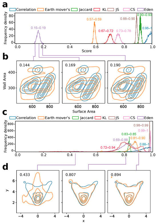
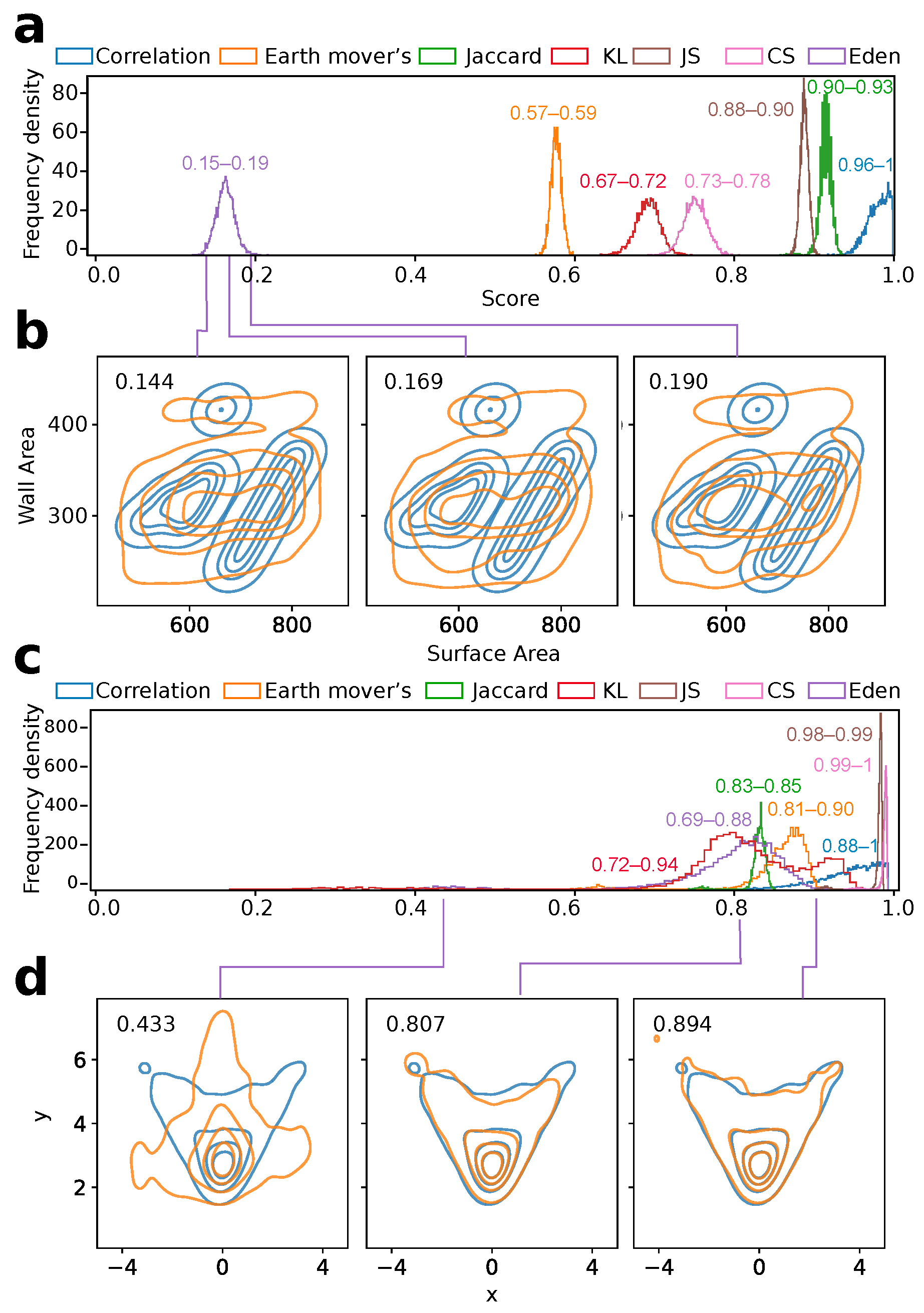
Our results support repeat sampling as a middle ground between sampling error and mismatch due to oversampling: i.e., scoring each sample and reporting summary statistics such as the mean ± standard deviation of the scores, the median, interquartile scores, or simply the nth percentile score. The latter is more conservative than the mean or median: it is the score that n percent of the scores are better than. Figure 7a,c show the distribution of values for each score for 5000 resamplings for the very low-quality fit from Figure 3a and the high-quality fit from Figure 3e, respectively. (Figure 7b,d show KDEs from different samples drawn from the range of scores for Eden). Notably, the score distributions spanned at least several percent for all seven scoring methods. The extent of the variation observed in Figure 7 supports caution in grading generative models. This strongly suggests that results from single samples can be misleading, may lack discriminative power, and therefore, should be avoided if possible.
Figure 7.
Confidence intervals. (a) Score distributions from 5000 repeat samples for the fit from Figure 3a, a very low-quality fit; 5th- and 95th-percentile limits shown. Note, all 5000 samples are from the same fit. (b) Representative KDE plots for samples drawn (purple lines) from different parts of the Eden score distribution (with Eden scores shown). (c) Score distributions from 5000 repeat samples for the fit from Figure 3e, a high-quality fit, with 5th- and 95th-percentile limits. Again, all 5000 samples are from the same fit. (d) Representative KDE plots for samples drawn from different parts of the Eden score distribution (with Eden scores shown).
4. Discussion
All modeling benefits from reliable quality scores, including the two-dimensional distributions resulting from generative models that are most often presented in print. Scores can mislead in several ways, including overfitting and in leading to selection of the wrong model [39]. Here, we add to these dangers the grade-inflation problem, named for a perennially-decried phenomenon in U.S. higher education [40], in which a statistic scores a model higher than it should and does not reflect true differences in performance. We describe why the commonly used correlation score should be particularly prone to grade inflation and offer examples from real-world datasets where many commonly used scores—specifically, the earth-mover’s, Jaccard, and KL scores—still have this problem, while at least one other score, our newly proposed Eden score, appears not to. We also show the value of multiple sampling for measuring and reporting confidence in these scores, which appears to be a relatively uncommon practice in the literature. We suspect the grade-inflation problem is not new but is made newly relevant by the explosive growth of data science, the need to select among high-performing models, the inability to keep up via human visual inspection, and the computational resources increasingly available for data visualization (for example, enabling pairwise scatter plots for ever higher-dimensional datasets).
It is interesting that the Eden score agrees substantially better with human perception of goodness-of-fit than the other scores tested, in a blind head-to-head comparison on data from generative models. This finding suggests that when human raters compare distributions for similarity, they, like the Eden score, might also be comparing distributions at multiple densities and subconsciously averaging the result. The caveats: raters were specifically asked to consider all contours, were shown the distributions as KDE plots (as opposed to, for example, as three-dimensional and/or interactive renderings), and were limited to people with scientific backgrounds. Application of Eden in other fields and contexts is an interesting direction for further investigation.
4.1. Equipoint vs. Equidensity Scores
What explains the difference between the earth-mover’s, Jaccard, KL, JS, and CS score on the one hand, which exhibited grade inflation, and Eden, which did not? One answer is that these two sets of scores differ qualitatively in how they weight different regions of the two distributions being compared. The earth-mover’s score weights each datapoint equally, regardless of where in a distribution that point lies. Because, by definition, there are more datapoints in areas of higher density, the earth-mover’s score will tend to be high as long as the regions of highest density line up well between the two distributions, almost regardless of how mismatched the low-density regions are (absent extreme outliers). The Jaccard and other divergence-based measures (KL, JS, and CS scores) also weight each datapoint equally, with similar results. Note, these scores are likely not the only ones with this property. For example, multi-dimensional extensions of the Kolmogorov–Smirnov (KS) statistic also seem to have this issue [41], and the Frechet inception distance is likely to suffer grade inflation as well, since it is based on the earth-mover’s distance. We see no obvious reason that scoring methods based on other f-divergences would not also have this problem. We coin the term “equipoint” for scores of this kind. Based on these examples, we hypothesize that all equipoint scores will suffer from this tyranny of the majority, yielding high scores even when low-density regions are poorly fit, resulting in grade inflation (Figure 3 and Table 2).
In contrast, the Eden score weights datapoints unequally, such that all densities contribute equally to the score. In such “equidensity” scores, the region of lowest density carries equal weight to the region of highest density and, indeed, to all density regions in between (Figure 4). Topologically, both the peaks and the foothills of the real and synthetic distributions have to line up well to obtain a high equidensity score, whereas only the peaks need to line up to obtain high equipoint scores. We propose that equidensity scores such as Eden should be preferred whenever accuracy is required throughout the distribution. (We exclude “unreasonable” equidensity scores from consideration, e.g., taking a trivially large nth root of Eden such that all scores end up arbitrarily close to 1). For example, for medical applications, it is often just as important that generative models accurately capture the features of rare presentations (foothills) as common ones (peaks) [7]. Since one of the main purposes of generative models is to fill out rare cases, we conclude that equidensity scores will generally have the advantage over equipoint scores for this application. Although, to our knowledge, the Eden score is the first equidensity score, or at least the first recognized as such, it is possible that scores based on other measures that up-weight tails also have something of an equidensity character; potential examples include the one-dimensional Anderson–Darling statistic, which up-weights tails more than the KS and, e.g., Cramér–von Mises statistics and which can be extended to two dimensions [42]. This is a topic for future study.
4.2. Score Calibration
Like all scores, equidensity scores can be calibrated to a desired range of values, for example, by raising to an exponent (for scores that range from 0 and 1). Importantly, note that for a given scoring statistic, calibration cannot change which of two fits has the higher value. For example, no calibration procedure can make the correlation score for Figure 3e larger than for Figure 3a (Table 2). This is a structural problem with the correlation score; as we have shown, it affects the equipoint scores as well. This means that even though all correlation scores can be brought arbitrarily low in hopes of resolving the absolute grade inflation they exhibit, for example by raising the correlation score to a sufficiently large exponent, structurally, the correlation score will still always exhibit relative grade inflation, in which low-quality fits will perform as well as or better than high-quality ones. Thus, calibration cannot fix grade inflation. The goal of the present work has been to investigate scores’ structural properties. Calibration of the Eden score or other scores, if desired, is left for future work.
4.3. Sampling Error and Confidence
It is interesting to find that confidence intervals were not negligible (Figure 7). In several of the examples we investigated, even the inter-quartile ranges, much less the 5th–95th percentile ranges, exceeded the differences between mean values for scores on the example fits in Figure 3. This observation is potentially important for comparing models: if the score used is one whose confidence interval is comparable to or even wider than the difference in score values between two models, one might mistake the worse model for the better one, or conclude a difference when no statistically significant difference exists. We note that in the machine-learning literature, model performance is often compared out to several decimal places without confidence intervals being reported. Figure 7 suggests interpreting such results with caution.
Consideration of variance raises the question of whether the Eden score should always be calculated with five annuli. In Appendix B, we study how the Eden score varies with the number of annuli and show that the score decreases to zero as the number of annuli grows. We propose that the correct choice of the contour number should depend on the total number of data points, such that sufficiently many points lie in each annulus to provide for acceptable sampling variation and acceptable confidence intervals. Because sampling error scales as the root of the number of points, we suggest one approach is to choose the number of annuli so that there are at least roughly 30 points per annulus; more points per annulus will result in narrower confidence intervals, but more annuli will result in a higher-resolution comparison of the two distributions. We believe this is essentially a bias–variance trade-off, which is the choice of the investigator. (In this study, we used five annuli throughout to control for any effects variation in this choice might have). For general applications beyond synthetic data in which the number of points is non-limiting—for example, when the two distributions are continuous and defined at every point—it could be interesting to define a continuum limit for . This is left for future work.
4.4. Connections to Entropy and Diversity
The correspondence between unequal weighting at the level of datapoints and equal weighting at the level of densities has an interesting connection to entropy and diversity, specifically to the Rényi entropies and the corresponding Hill diversities . (Here, , a potentially confusing but purely notational difference reflecting the conventions in the respective literature; in this work, we distinguish q the viewpoint parameter from q the distribution by context). Both and can be interpreted as sums of the frequencies of species in a system, with q as a frequency-weighting parameter such that rarer species contribute less as q rises. is used to calculate the “effective number” of species in a population, taking frequencies into account to a degree q. It has been observed [36,43,44] that many commonly used statistics correspond to positive integer values of q. For example, corresponds to a simple count of the number of unique species, corresponds to the Shannon entropy, corresponds to Simpson’s index, and so on up to , which corresponds to the Berger–Parker index [45]. (These correspondences generally take the form of simple mathematical transformations of ).
q () can also take negative values; however, entropies/diversities with negative have received little if any attention in the literature, perhaps owing to a dearth of real-world examples for [46]. We broach the possibility that equidensity scores might be interpreted as an example of negative if one considers the species in the entropy calculation to be datapoints and that there is a duality with if instead one considers the species to be equidensity regions (i.e., annuli/rings/topological contours). Note this is qualitatively different from how negative operates in the Rényi divergences, which is to swap distributions p and q (to a reasonable approximation, increasingly true the further from ). Insofar as equidensity regions are groupings or “communities” of datapoints, there may also be connections with the subcommunity/metacommunity formulation in the diversity literature [47] that correspond to concepts such as relative/joint entropy and mutual information in the entropy literature [36]. We note that a Python package already exists that accepts negative [48]. Finally, we note that information-theoretic tools have been applied to characterize datasets using representations other than points or densities, e.g., using spectra of matrices [49]. Exploring such connections could be an interesting direction for future work.
4.5. Use Cases and Exceptions
The general use case for the Eden score is to compare pairs of two-dimensional, i.e., pairwise, distributions. As we have shown, this makes it highly applicable for generative modeling and for two-dimensional pairwise comparisons more generally. We propose that Eden could also be useful for comparing pairs of three-dimensional distributions but caution that comparisons in still-higher dimensions could incur the curse of dimensionality.
The question arises of whether there are two-dimensional cases where Eden might not be preferred. We believe there are at least two such cases. The first is where there is a strong prior on the two-dimensional data, for example, when the expectation is that the data follow a simple line or curve. For example, suppose each of the two distributions is expected to lie on a simple straight line. In such cases, a regression-based score such as the correlation score can potentially still be useful; however, as Anscombe showed, it is still worth approaching with caution [13].
The second case where Eden might not be preferred is when the data configuration is very highly constrained. For example, in the extreme case where each feature is a binary variable (Boolean data), the space of possibilities consists of only four possible points: the coordinates (0, 0), (0, 1), (1, 0), and (1, 1). This constraint leaves no meaningful density regions as such. As a result, equidensity scores are unlikely to be of benefit. In such cases, an alternative approach is to treat the four coordinates as categoricals and score agreement between the resulting two distributions accordingly. In contrast, Eden is for the general use case of complex and/or non-parametric data defining meaningful densities in two dimensions. Potential additional use cases and limitations are left for future investigation.
4.6. Conclusions and Limitations
In this work, we have identified the common grade inflation problem in evaluating synthetic data from generative models. We have introduced the Eden score, a novel equidensity score that weighs datapoints unequally, such that all densities contribute equally to the score. Our results demonstrate that the Eden score outperforms other widely used scores, such as the correlation score and earth-mover’s score, in accurately measuring goodness-of-fit for generative models. We propose that equidensity scores like the Eden score should be preferred in applications where accuracy is required throughout the distribution, such as in medical applications where rare cases are just as important as common ones. We also highlight the importance of considering the structural properties of scores and the need for more robust evaluation metrics in the field of generative modeling.
For the simplicity of visual inspection, this work only represented contours for raters to compare the goodness-of-fit of two synthetic data. One direction for followup studies is more extensive human testing, including testing for dependency on scientific vs. lay background, different instructions (e.g., “choose the better fit”), different types of visualization (e.g., scatterplots). Such studies would further validate the Eden score’s robustness in general settings.
The primary limitations of this work are its focus on two-dimensional distributions and its evaluation of a relatively small number of scoring methods—notwithstanding these appear to be the most common methods in use. In particular, it does not investigate the behavior of Eden or other equidensity scores in higher dimensions, nor does it systematically discover or evaluate alternative equidensity scores. How a one-dimensional version of the Eden score would compare to the KS statistic or a one-dimensional KL score is also an interesting open question.
Although the Eden construction can in principle be extended to higher-dimensional distributions, its behavior in high dimensions remains an open question. As dimensionality increases, we expect the curse of dimensionality to affect both the estimation of the underlying density and the geometric overlap of corresponding equidensity regions. In particular, as with the Jaccard score, relatively small discrepancies between two distributions can produce increasingly small intersection-over-union values because high-dimensional volumes can separate rapidly. Consequently, the higher-dimensional Eden score may yield artifactually low scores in sufficiently high dimensions, even when the underlying distributions might reasonably be regarded as similar. Investigating this possibility is left for future work. Studies of higher dimensions might be considered useful, since non-trivial real datasets are often high-dimensional (e.g., many columns), but using human raters as standard would be complicated by the inability to easily visualize higher dimensions and by potentially important losses if dimensionality reduction is used (e.g., PCA [8], tSNE [10], UMAP [9], or the more recently proposed MAP IT [50]). Fortunately, lower-order relationships often carry a large amount of information about the configuration of complex systems [15,16]. For this reason, we expect Eden and other equidensity scores to be useful additions to the generative-modeling toolkit.
Author Contributions
Conceptualization, R.A. (Ramy Arnaout); methodology, P.N., M.L., A.M., R.A. (Rima Arnaout), and R.A. (Ramy Arnaout); software, P.N., M.L., and A.M.; writing, P.N., M.L., A.M., R.A. (Rima Arnaout), and R.A. (Ramy Arnaout). All authors have read and agreed to the published version of the manuscript.
Funding
This work was supported by the Gordon and Betty Moore Foundation, the Food and Drug Administration, and the NIH under grants R01HL150394, R01HL150394-SI, R01AI148747, and R01AI148747-SI.
Institutional Review Board Statement
This study is IRB exempt based on Code of Federal Regulation (45 CFR 46.104(d)(4)(ii)).
Informed Consent Statement
Not applicable.
Data Availability Statement
Data are made available in https://github.com/ArnaoutLab/Grade-Inflation/ (accessed 15 October 2026).
Conflicts of Interest
The authors declare no conflicts of interest.
Appendix A. Python Implementation of the Eden Score
In this appendix, we present a Python implementation of the Eden score.
Box A1. An Eden score implementation
import numpy as np
import pandas as pd
import matplotlib
import matplotlib.pyplot as plt
from scipy.stats import gaussian_kde

class FastEdenScorer:
    ‘‘""Scores the similarity between two datasets via the overlap of their
    likelihood-density annuli (Eden score).
    ’’""

    def __init__(
        self,
        n_of_levels: int = 5,
        thresh: float = 0.05,
        size: int = 50000,
        seed: int | None = None,
        debug: bool = False,
        cut: int = 5,
        edge_exp: float = 0.05,
        bw_method: str | float | None = None,
    ) -> None:
        self.n_of_levels = n_of_levels
        self.thresh = thresh
        self.size = size
        self.seed = seed
        self.debug = debug
        self.cut = cut
        self.edge_exp = edge_exp
        self.bw_method = bw_method
        self.make_quantiles()

    def make_quantiles(self) -> None:
        array_of_quantiles = np.arange(
            self.thresh, 1, (1 - self.thresh)/(self.n_of_levels - 1)
        )
        array_of_quantiles = np.concatenate(([0], array_of_quantiles))
        self.array_of_quantiles = np.concatenate((array_of_quantiles, [1]))

    class DataDist:
        def __init__(
            self,
            data: pd.DataFrame,
            sampling_size: int,
            bw_method: str | float | None = None,
            seed=None,
        ) -> None:
            self.original_data = data
            self.data_no_na = self.original_data.dropna()
             # NOTE: bw_method now honors 'scott', 'silverman', or a scalar
            self.kernel = gaussian_kde(
                self.data_no_na.T, bw_method=bw_method
            )
            if seed is not None:
                np.random.seed(seed)
            self.resample = self.kernel.resample(size=sampling_size)
            self.likelihoods = self.kernel.evaluate(self.resample)
            # likelihood of the *actual* (non-resampled) data points, used for
            # the ‘‘number of data points in each annulus'' diagnostic
            self.likelihoods_of_data = self.kernel.evaluate(
                self.data_no_na.to_numpy().T
            )

        def make_bins(self, quantiles: np.ndarray) -> None:
            _, self.likelihoods_bins = pd.qcut(
                self.likelihoods, quantiles, retbins=True, duplicates='drop'
            )

        def make_contours(self) -> None:
            self.outermost_contour = self.resample.T[
                np.isclose(
                    self.likelihoods,
                    self.likelihoods_bins[1],
                    atol=self.likelihoods_bins[1]/100,
                )
            ]
            self.outermost_contour_min = np.array(
                [
                    np.min(self.outermost_contour[:, 0]),
                    np.min(self.outermost_contour[:, 1]),
                ]
            )
            self.outermost_contour_max = np.array(
                [
                    np.max(self.outermost_contour[:, 0]),
                    np.max(self.outermost_contour[:, 1]),
                ]
            )

        def make_uniform_sample_likelihoods(self, uniform_sample: np.ndarray) -> None:
            self.likelihoods_of_uniform_sample = self.kernel.evaluate(
                uniform_sample.T
            )

        def make_uniform_sammple_likelihoods(self, uniform_sample):
            self.make_uniform_sample_likelihoods(uniform_sample)

    class GraphicResult:
        def __init__(
            self,
            Eden_score: np.float64,
            outermost_contour_min: np.ndarray,
            outermost_contour_max: np.ndarray,
            real_likelihoods_bins: np.ndarray,
            syn_likelihoods_bins: np.ndarray,
            kernel_real: gaussian_kde,
            kernel_syn: gaussian_kde,
            jaccard_scores: list | None = None,
            real_annulus_counts: list | None = None,
            syn_annulus_counts: list | None = None,
            intersection_counts: list | None = None,
            union_counts: list | None = None,
            n_real_points: int | None = None,
            n_syn_points: int | None = None,
            bw_method: str | float | None = None,
        ) -> None:
            self.EdenScore = Eden_score
            self.outermost_contour_min = outermost_contour_min
            self.outermost_contour_max = outermost_contour_max
            self.real_likelihoods_bins = real_likelihoods_bins
            self.syn_likelihoods_bins = syn_likelihoods_bins
            self.kernel_real = kernel_real
            self.kernel_syn = kernel_syn
            self.jaccard_scores = jaccard_scores or []
            self.real_annulus_counts = real_annulus_counts or []
            self.syn_annulus_counts = syn_annulus_counts or []
            self.intersection_counts = intersection_counts or []
            self.union_counts = union_counts or []
            self.n_real_points = n_real_points
            self.n_syn_points = n_syn_points
            self.bw_method = bw_method

    def score(
        self,
        real_data: pd.DataFrame,
        syn_data: pd.DataFrame,
        return_more: bool = False,
    ) -> GraphicResult | np.float64:
        if self.seed is not None:
            np.random.seed(self.seed)

        real = self.DataDist(real_data, self.size, self.bw_method, seed=self.seed)
        syn = self.DataDist(syn_data, self.size, self.bw_method, seed=self.seed)

        for dist in (real, syn):
            dist.make_bins(self.array_of_quantiles)
            dist.make_contours()

        outermost_contour_min = np.minimum(
            real.outermost_contour_min, syn.outermost_contour_min
        )
        outermost_contour_max = np.maximum(
            real.outermost_contour_max, syn.outermost_contour_max
        )

        outermost_contour_range = outermost_contour_max - outermost_contour_min
        low_edge, high_edge = (
            outermost_contour_min - self.edge_exp * outermost_contour_range,
            outermost_contour_max + self.edge_exp * outermost_contour_range,
        )
        uniform_sample = np.random.uniform(
            low=low_edge, high=high_edge, size=(self.size, real_data.shape[1])
        )
        for dist in (real, syn):
            dist.make_uniform_sample_likelihoods(uniform_sample)

        jaccard_scores = []
        real_annulus_counts, syn_annulus_counts = [], []
        intersection_counts, union_counts = [], []

        for i in range(self.n_of_levels - 1):
            lower_real_bin_edge, upper_real_bin_edge = (
                real.likelihoods_bins[i + 1],
                real.likelihoods_bins[i + 2],
            )
            lower_syn_bin_edge, upper_syn_bin_edge = (
                syn.likelihoods_bins[i + 1],
                syn.likelihoods_bins[i + 2],
            )

            in_real_annulus = (
                (lower_real_bin_edge <= real.likelihoods_of_uniform_sample)
                & (real.likelihoods_of_uniform_sample <= upper_real_bin_edge)
            )
            in_syn_annulus = (
                (lower_syn_bin_edge <= syn.likelihoods_of_uniform_sample)
                & (syn.likelihoods_of_uniform_sample <= upper_syn_bin_edge)
            )

            union_criterion = in_real_annulus | in_syn_annulus
            intersection_criterion = in_real_annulus & in_syn_annulus

            union = uniform_sample[union_criterion]
            intersection = uniform_sample[intersection_criterion]

            if len(union) == 0:  # can happen at extreme thresh/level settings
                jaccard = np.nan
            else:
                jaccard = len(intersection)/len(union)

            jaccard_scores.append(jaccard)
            union_counts.append(len(union))
            intersection_counts.append(len(intersection))

            # actual (non-resampled) data points falling in each annulus
            real_annulus_counts.append(
                int(
                    (
                        (lower_real_bin_edge <= real.likelihoods_of_data)
                        & (real.likelihoods_of_data <= upper_real_bin_edge)
                    ).sum()
                )
            )
            syn_annulus_counts.append(
                int(
                    (
                        (lower_syn_bin_edge <= syn.likelihoods_of_data)
                        & (syn.likelihoods_of_data <= upper_syn_bin_edge)
                    ).sum()
                )
            )

        Eden_score = np.float64(np.nanmean(jaccard_scores))

        return Eden_score
Appendix B. Hyperparameter Sensitivity Analysis
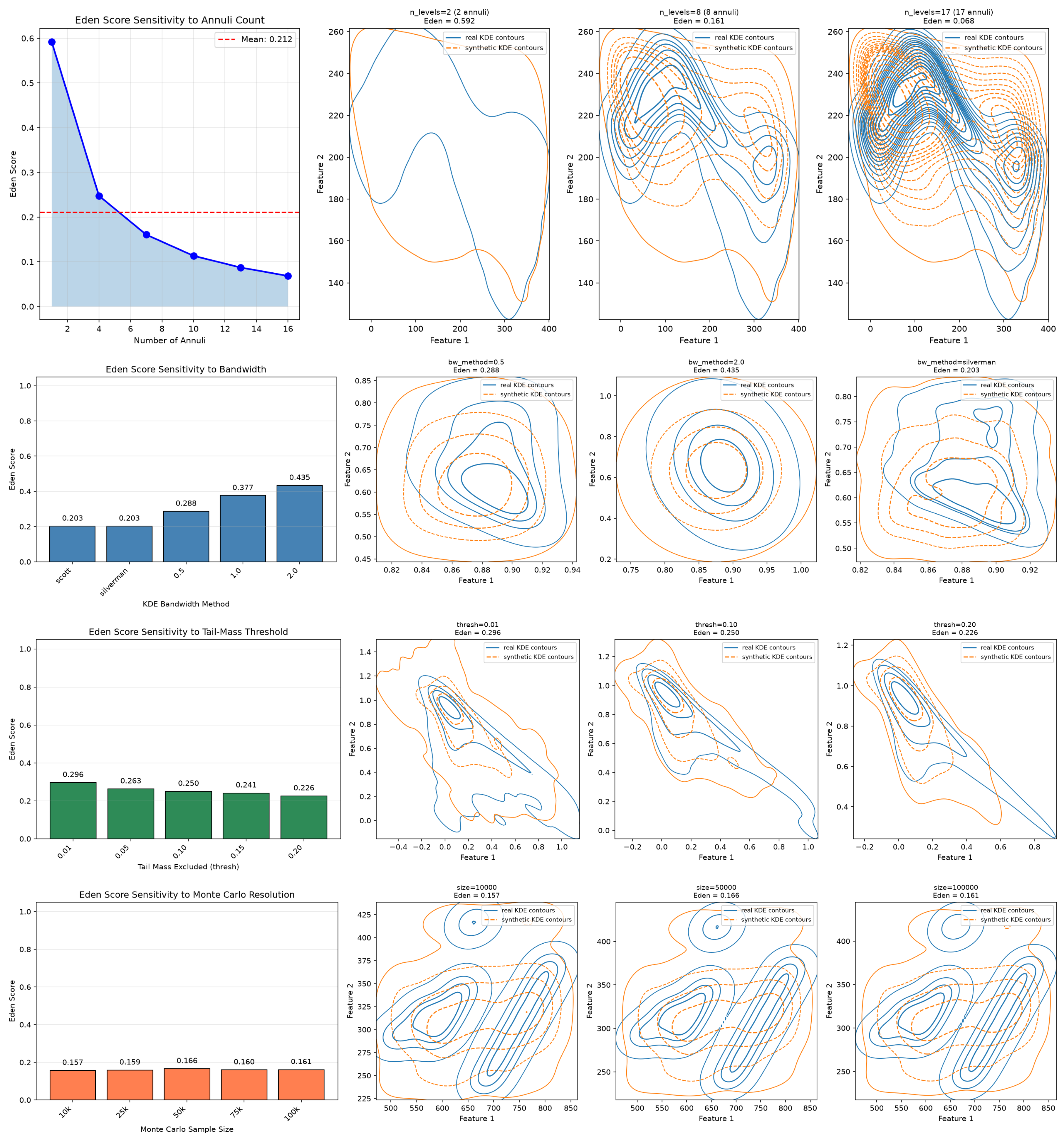
In this appendix, we study how much the Eden score varies with each of the four hyperparameters: number of levels (n_of_levels in the implementation above), bandwidth (bw_method), threshold for tail-mass exclusion (thresh), and number of Monte-Carlo points (size). Each study will vary one hyperparameter while holding the others at their default values (n_of_levels = 5, bw_method = ’scott’, thresh = 0.05, size = 50,000). To probe different aspects of the score, each study uses a different real/synthetic pair from Figure 2: the annuli study uses Covertype (GC), the bandwidth study uses Rice (CTGAN), the threshold study uses Communities and Crime (nFlow), and the Monte-Carlo study uses Energy Efficiency (TVAE). Results are shown in Figure A1.
Appendix B.1. Number of Annuli
The Eden score decreases monotonically with the number of levels, from 0.59 at n_of_levels = 2 to 0.07 at n_of_levels = 17, with the largest drop occurring between 2 and 8 levels. This behavior is expected: with few annuli, coarse resolution averages away fine-scale mismatches between the two distributions, so the score is inflated. As the number of annuli tends to infinity, we generically expect the Eden score to go to zero; this is because the intersection between any two annuli becomes more and more point-like and, hence, have much smaller area than the union of the two annuli. We recommend reporting the number of annuli alongside the Eden score.
Figure A1.
Sensitivity of the Eden score to the number of annuli (top row), the KDE bandwidth (second row), the tail-mass threshold (third row), and the number of Monte-Carlo points (last row).
Appendix B.2. KDE Bandwidth
The commonly used adaptive rules for the bandwidth (Scott’s and Silverman’s) both yield an Eden score of 0.20. Fixed bandwidth factors inflate the score more and more as the factor grows: 0.29 at factor 0.5, 0.38 at factor 1.0, and 0.44 at factor 2.0. Inspection of the contour panels confirms the cause: at large bandwidths, the KDE smears away the hard edge structure in the dataset dataset, and both the real and synthetic densities become single smooth blobs that overlap well, inflating the score. We therefore recommend adaptive bandwidth selection, which is also the default of most KDE implementations.
Appendix B.3. Tail-Mass Threshold
The Eden score decreases slowly and monotonically as the threshold increases, from 0.30 at thresh = 0.01 to 0.23 at thresh = 0.20. We note that at very low thresholds, the contours become irregular due to outliers, which makes their shapes not reliable. Thus, we recommend using a threshold at least as large as the default value.
Appendix B.4. Monte-Carlo Sample Size
The Eden score is nearly constant across sample sizes ranging from 10,000 to 100,000 points (all values within 0.157–0.166). The estimator therefore converges well below the default of size = 50,000, and this hyperparameter can safely be reduced when computation time matters.
In summary, the Eden score is mildly sensitive to the Monte-Carlo sample size and the tail-mass threshold, while it responds more strongly to the number of annuli and to KDE over-smoothing.
References
- Miao, B.Y.; Chen, I.Y.; Williams, C.Y.K.; Davidson, J.; Garcia-Agundez, A.; Sun, S.; Zack, T.; Saria, S.; Arnaout, R.; Quer, G.; et al. The Minimum Information about CLinical Artificial Intelligence Checklist for Generative Modeling Research (MI-CLAIM-GEN). arXiv 2024, arXiv:2403.02558. [Google Scholar]
- Bauer, A.; Trapp, S.; Stenger, M.; Leppich, R.; Kounev, S.; Leznik, M.; Chard, K.; Foster, I. Comprehensive Exploration of Synthetic Data Generation: A Survey. arXiv 2024, arXiv:2401.02524. [Google Scholar]
- Beaulieu-Jones, B.K.; Wu, Z.S.; Williams, C.; Lee, R.; Bhavnani, S.P.; Byrd, J.B.; Greene, C.S. Privacy-Preserving Generative Deep Neural Networks Support Clinical Data Sharing. Circ. Cardiovasc. Qual. Outcomes 2019, 12, e005122. [Google Scholar] [CrossRef] [Scilit] [PubMed]
- Ge, K.; Nguyen, P.; Arnaout, R. lucie: An Improved Python Package for Loading Datasets from the UCI Machine Learning Repository. bioRxiv 2024. [Google Scholar] [CrossRef] [Scilit] [PubMed]
- Tkachenko, N. Opportunities for synthetic data in nature and climate finance. Front. Artif. Intell. 2024, 6, 1168749. [Google Scholar] [CrossRef] [Scilit] [PubMed]
- Arnaout, R. Adapting vision-language AI models to cardiology tasks. Nat. Med. 2024, 30, 1245–1246. [Google Scholar] [CrossRef] [Scilit] [PubMed]
- Dey, D.; Arnaout, R.; Antani, S.; Badano, A.; Jacques, L.; Li, H.; Leiner, T.; Margerrison, E.; Samala, R.; Sengupta, P.P.; et al. Proceedings of the NHLBI Workshop on Artificial Intelligence in Cardiovascular Imaging: Translation to Patient Care. Jacc Cardiovasc. Imaging 2023, 16, 1209–1223. [Google Scholar] [PubMed]
- Jolliffe, I.T.; Cadima, J. Principal component analysis: A review and recent developments. Philos. Trans. R. Soc. A Math. Phys. Eng. Sci. 2016, 374, 20150202. [Google Scholar] [CrossRef] [Scilit] [PubMed]
- McInnes, L.; Healy, J.; Melville, J. UMAP: Uniform Manifold Approximation and Projection for Dimension Reduction. arXiv 2020, arXiv:1802.03426. [Google Scholar]
- Maaten, L.v.; Hinton, G. Visualizing Data using t-SNE. J. Mach. Learn. Res. 2008, 9, 2579–2605. [Google Scholar]
- Shmelkov, K.; Schmid, C.; Alahari, K. How Good Is My GAN? In Computer Vision—ECCV 2018; Ferrari, V., Hebert, M., Sminchisescu, C., Weiss, Y., Eds.; Springer International Publishing: Cham, Switzerland, 2018; pp. 218–234. [Google Scholar]
- DataCebo, Inc. Synthetic Data Metrics, version 0.11.0; DataCebo, Inc.: Boston, MA, USA, 2024. [Google Scholar]
- Anscombe, F.J. Graphs in Statistical Analysis. Am. Stat. 1973, 27, 17–21. [Google Scholar] [CrossRef] [Scilit]
- Matejka, J.; Fitzmaurice, G. Same Stats, Different Graphs: Generating Datasets with Varied Appearance and Identical Statistics through Simulated Annealing. In Proceedings of the 2017 CHI Conference on Human Factors in Computing Systems, Denver, CO, USA, 6–11 May 2017; ACM: New York, NY, USA, 2017; pp. 1290–1294. [Google Scholar]
- Bialek, W.; Ranganathan, R. Rediscovering the power of pairwise interactions. arXiv 2007, arXiv:0712.4397. [Google Scholar]
- Schneidman, E.; Berry, M.J.; Segev, R.; Bialek, W. Weak pairwise correlations imply strongly correlated network states in a neural population. Nature 2006, 440, 1007–1012. [Google Scholar] [CrossRef] [Scilit] [PubMed]
- Charpentier, A.; Fermanian, J.; Scaillet, O. The Estimation of Copulas: Theory and Practice. In Copulas: From Theory to Application in Finance; Rank, J., Ed.; Bloomberg Press: New York, NY, USA, 2006; pp. 35–64. [Google Scholar]
- Xu, L.; Skoularidou, M.; Cuesta-Infante, A.; Veeramachaneni, K. Modeling Tabular data using Conditional GAN. arXiv 2019, arXiv:1907.00503. [Google Scholar]
- Xu, L. Synthesizing Tabular Data Using Conditional GAN. Master Thesis, Massachusetts Institute of Technology, Cambridge, MA, USA, 2020. [Google Scholar]
- Stimper, V.; Liu, D.; Campbell, A.; Berenz, V.; Ryll, L.; Schölkopf, B.; Hernández-Lobato, J.M. normflows: A pytorch package for normalizing flows. J. Open Source Softw. 2023, 8, 5361. [Google Scholar] [CrossRef] [Scilit]
- Couch, J.; Arora, R.; Braun, J.; Kaplinsky, J.; Hill, E.; Li, A.; Altschul, B.; Arnaout, R. Scaling Monte-Carlo-Based Inference on Antibody and TCR Repertoires. arXiv 2023, arXiv:2312.12525. [Google Scholar]
- Waskom, M. seaborn: Statistical data visualization. J. Open Source Softw. 2021, 6, 3021. [Google Scholar] [CrossRef] [Scilit]
- Kim, J.; Scott, C.D. L2 kernel classification. IEEE Trans. Pattern Anal. Mach. Intell. 2010, 32, 1822–1831. [Google Scholar] [CrossRef] [Scilit] [PubMed]
- Kullback, S.; Leibler, R.A. On information and sufficiency. Ann. Math. Stat. 1951, 22, 79–86. [Google Scholar] [CrossRef] [Scilit]
- Kantorovich, L.V. Mathematical Methods of Organizing and Planning Production. Manag. Sci. 1960, 6, 366–422. [Google Scholar] [CrossRef] [Scilit]
- Mallows, C.L. A Note on Asymptotic Joint Normality. Ann. Math. Stat. 1972, 43, 508–515. [Google Scholar] [CrossRef] [Scilit]
- Rubner, Y.; Tomasi, C.; Guibas, L.J. A metric for distributions with applications to image databases. In Proceedings of the Sixth International Conference on Computer Vision (IEEE Cat. No. 98CH36271), Bombay, India, 7 January 1998; Narosa Publishing House: New Delhi, India, 1998; pp. 59–66. [Google Scholar]
- Vaserstein, L.N. Markov processes over denumerable products of spaces, describing large systems of automata. Probl. Peredachi Informatsii 1969, 5, 64–72. [Google Scholar]
- Flamary, R.; Nicolas Courty, N.; Alexandre Gramfort, A.; Alaya, M.Z.; Boisbunon, A.; Chambon, S.; Chapel, L.; Corenflos, A.; Fatras, K.; Fournier, N.; et al. POT: Python Optimal Transport. J. Mach. Learn. Res. 2024, 22, 1–8. [Google Scholar]
- Jaccard, P. Étude comparative de la distribution florale dans une portion des Alpes et du Jura. Bull. Soc. Vaudoise Sci. Nat. 1901, 37, 547–579. [Google Scholar]
- Jaccard, P. The Distribution of The Flora in the Alpine Zone. New Phytol. 1912, 11, 37–50. [Google Scholar] [CrossRef] [Scilit]
- Lin, J. Divergence measures based on the Shannon entropy. IEEE Trans. Inf. Theory 1991, 37, 145–151. [Google Scholar] [CrossRef] [Scilit]
- Principe, J.C.; Xu, D.; Fisher, J.; Haykin, S. Information Theoretic Learning; IEEE: New York, NY, USA, 2006. [Google Scholar]
- Heusel, M.; Ramsauer, H.; Unterthiner, T.; Nessler, B.; Hochreiter, S. GANs Trained by a Two Time-Scale Update Rule Converge to a Local Nash Equilibrium. arXiv 2018, arXiv:1706.08500. [Google Scholar]
- Pele, O.; Werman, M. Fast and robust earth-mover’s distances. In 2009 IEEE 12th International Conference on Computer Vision; IEEE: New York, NY, USA, 2009; pp. 460–467. [Google Scholar]
- Leinster, T. Entropy and Diversity: The Axiomatic Approach. arXiv 2024, arXiv:2012.02113. [Google Scholar]
- CallumMcDougall. Six (and A Half) Intuitions for KL Divergence. 2022. Available online: https://www.lesswrong.com/posts/no5jDTut5Byjqb4j5/six-and-a-half-intuitions-for-kl-divergence?utm_source=chatgpt.com (accessed on 15 October 2026).
- Landis, R.J.; Koch, G.G. The Measurement of Observer Agreement for Categorical Data. Biometrics 1977, 33, 159–174. [Google Scholar] [CrossRef] [Scilit]
- Greene, A.L.; Eaton, N.R.; Forbes, M.K.; Fried, E.I.; Watts, A.L.; Kotov, R.; Krueger, R.F. Model fit is a fallible indicator of model quality in quantitative psychopathology research: A reply to Bader and Moshagen. J. Psychopathol. Clin. Sci. 2022, 131, 696–703. [Google Scholar] [CrossRef] [Scilit] [PubMed]
- Grade inflation—Wikipedia, the Free Encyclopedia, December 2024. Page Version ID: 1262760765. Available online: https://en.wikipedia.org/wiki/Grade_inflation (accessed on 15 October 2026).
- Harrison, D.; Sutton, D.; Carvalho, P.; Hobson, M. Validation of Bayesian posterior distributions using a multidimensional Kolmogorov–Smirnov test. arXiv 2015, arXiv:1404.7735. [Google Scholar]
- Anderson, T.W.; Darling, D.A. Asymptotic Theory of Certain “Goodness of Fit” Criteria Based on Stochastic Processes. Ann. Math. Stat. 1952, 23, 193–212. [Google Scholar]
- Hill, M.O. Diversity and Evenness: A Unifying Notation and Its Consequences. Ecology 1973, 54, 427–432. [Google Scholar] [CrossRef] [Scilit] [PubMed]
- Jost, L. Entropy and diversity. Oikos 2006, 113, 363–375. [Google Scholar] [CrossRef] [Scilit]
- Berger, W.H.; Parker, F.L. Diversity of Planktonic Foraminifera in Deep-Sea Sediments. Science 1970, 168, 1345–1347. [Google Scholar] [CrossRef] [Scilit] [PubMed]
- Li, Y.; Turner, R.E. Rényi Divergence Variational Inference. arXiv 2016, arXiv:1602.02311. [Google Scholar]
- Reeve, R.; Leinster, T.; Cobbold, C.A.; Thompson, J.; Brummitt, N.; Mitchell, S.N.; Matthews, L. How to partition diversity. arXiv 2016, arXiv:1404.6520. [Google Scholar]
- Nguyen, P.; Couch, J.; Bansal, R.; Morgan, A.; Tam, C.; Li, M.; Arnaout, R.; Arnaout, R. Comparing frameworks for similarity-aware generalized entropy (sentropy). Phys. Rev. E 2026, 113, 055305. [Google Scholar] [CrossRef] [Scilit] [PubMed]
- Yu, S.; Giraldo, L.G.S.; Jenssen, R.; Principe, J.C. Multivariate extension of matrix-based Rényi’s α-order entropy functional. IEEE Trans. Pattern Anal. Mach. Intell. 2019, 42, 2960–2966. [Google Scholar] [CrossRef] [Scilit] [PubMed]
- Jenssen, R. MAP IT to visualize representations. In Proceedings of the International Conference on Learning Representations, Vienna, Austria, 7–11 May 2024; Volume 2024, pp. 21388–21422. [Google Scholar]

Disclaimer/Publisher’s Note: The statements, opinions and data contained in all publications are solely those of the individual author(s) and contributor(s) and not of MDPI and/or the editor(s). MDPI and/or the editor(s) disclaim responsibility for any injury to people or property resulting from any ideas, methods, instructions or products referred to in the content. |
© 2026 by the authors. Licensee MDPI, Basel, Switzerland. This article is an open access article distributed under the terms and conditions of the Creative Commons Attribution (CC BY) license.