


Abstract
To improve physical processes, domain experts use experimental test setups to gather data. After sampling, the data is analysed using a regression model, for example. The objective of this work is to investigate the performance of different combinations of sampling and machine learning methods under varying process characteristics that are previously known to the domain expert. This results in practical recommendations for users with limited expertise in machine learning. A large-scale combinatorial test setup consisting of polynomial surrogates as pseudo processes with the characteristics of variable count, complexity, process noise and position of the optimum was created. The sampling methods (Sobol, random, Bayesian optimisation and response surface methodology with additional G-optimal test points) were compared against twenty-six ML methods. The results indicate that the choice of ML method has a greater influence on global modelling accuracy than the choice of sampling method. However, strong interactions between sampling and ML method demonstrate that they should not be selected independently. Overall, the findings suggest that process noise eliminates the predictive quality of standard regression models used in statistical evaluation. Space-filling sampling methods generally provide reliable performance, while regularised polynomial, kernel-based, and additive models offer strong predictive accuracy across multiple scenarios.
1. Introduction and Motivation
Process modelling is used in mechanical engineering to minimise the need for experimental testing and to reduce costs. Multiple approaches, such as analytical or numerical modelling and machine learning, are commonly employed to accurately predict the responses of process input data [1]. The recurring procedure involves defining the process window to be explored, selecting a data sampling and regression method, and evaluating the different approaches. The selection is bound by the user’s knowledge of the advantages and disadvantages of the different methods. It is most likely that the user who applies the model results originates from a mechanical rather than a data analytics context. This creates a discrepancy between the application of complex sampling and regression methods and the process optimisation implemented in practice. It is therefore necessary to provide an overview of which data collection and modelling methods deliver the best results based solely on the machine operator’s prior knowledge of the underlying process. The resulting research question is: Which type of regression method models a physical process best, depending on data sampling method and process characteristics?
To address this, prior knowledge of physical processes is characterised in terms of the number of variables, degree of complexity, standard deviation of scatter, variable interactions and optimum location in the search space. These characteristics are transferred to randomly generated polynomials to function as surrogate processes. The functions are then sampled using random, space filling, adaptive sampling and classical design of experiments (DoE) hybrid sampling strategies. The data are modelled using global parametric smooth models, global additive basis-function models, kernel methods, local instance-based models, tree-based partition and model tree methods, tree ensembles, and bagging/gradient boosting and neural networks (NN).
The work is structured as follows.
In Section 1, the research question and scope are derived. Section 2 presents and compares the combined research fields of sampling and regression methods in machine learning known from computer science with the statistical evaluation known as DoE, which is most common in mechanical engineering. In Section 3, the methodology of the research is set up. This implies the explanation of polynomials as surrogates for mechanical processes, the functioning of the data collection methods and the different kinds of machine learning (ML) methods. Section 4 presents the computed results of the comparison. In Section 5, a meta model is trained to help the selection process. The results are presented in the form of a cheat sheet. Limitations of the work regarding the significance and the applicability are discussed in Section 6. The work concludes with an encouragement for future research in Section 7.
2. State of the Art
The first insight in this section is about how machine learning methods are commonly used in engineering. A meta-analysis of 86 papers shows that in the product innovation process especially, NNs are used to model data with 62.6% [2]. Mixed results are presented whether only one ML is used or multiple techniques are compared to model the same data. For example, Aboretti et al. found that only 7.5%, Tercan and Meisen state 51% of 81 papers and Kamiri and Mariga suggest that 98% of 100 papers compare different ML techniques for one task [2,3,4]. This approach has been continued in recent studies. El-Sanabary et al. improved the wear behaviour of metals [5]. They compared three basic regression methods on the basis that they work well together, without providing further detail on this claim. The DoE approach was used for effect analysis and as a mathematical model for optimising multiple objectives. Another study compared the performance of different ML models in predicting the mechanical properties of fibre composites [6]. The authors justify the use of multiple ML methods, as current studies lack comparisons of regression methods for the given process. For this purpose, different representatives of model characteristics are selected. For the first take away, it is argued that the diverse results indicate a lack of definitive selection criteria of ML methods for practical applications.
The second insight to be given is the selection process of ML methods for a specific problem. Commonly, the task at hand limits the choice. Typically available ML subgroups are regression, classification and clustering [7], but other selection criteria are available and overlapping, such as supervised and unsupervised [8] or dimensionality reduction and anomaly detection ML methods [9]. The focus of this work is regression, so these selection criteria are further evaluated. Different approaches are taken to rank and order the methods. For example, Kumar et al. provide a table of ML methods applicable to criteria such as feature noise, size of the training data and outlier handling, and support their claims with relevant literature [9]. One research group uses publicly available test datasets with a median sample size of 1030 and benchmarks 10 ML methods [10]. In contrast, 164 ML methods are compared with datasets with a median of 1461 samples [11]. The researchers presented use an extensive sample size, which tends to be expensive in the data gathering process in physical experiments. For comparison, an analysis of 47 papers on experimental real datasets showcases that the median of available samples was 144 [3]. The conclusion here is that as the most applications for ML methods involve experimental data [3], a sample size of thousands of samples is mostly not feasible in an experimental setup. The sample size needed depends heavily on the complexity and dimensionality of the modelled process, consistent with the exponential growth of search spaces observed in NP-hard problems [12]. That said, increased sample size is exponentially associated with less absolute difference in the performance of regression ML methods regarding accuracy and standard deviation [13]. The conclusion is that the challenge is to select the ML method with the minimal sample size to describe the problem, for which this work provides an insight. This minimalistic approach also eliminates ML models like deep learning techniques for further evaluation, as they are known to be data-hungry. The take-away of this part of the research review is that the validity of the ranked ML performance is compromised if a large amount of training data is used without contextualising it in the complexity of the problem in question. On average, in an industrial setting, a large sample size cannot be replicated. Using current rankings as selection basis can therefore be misleading and result in sunk experimental costs.
As further insight, the sampling and the quality of the acquired data are reviewed. Data collection in ML is a critical step as it is most time consuming and therefore costly [14]. In addition, the completeness of the tabular data and the feature and response accuracy have been shown to have the most negative effect on the performance of regression models [15]. Due to the sensitivity of the data gathering step, another element to be considered is the sampling method used. Sampling strategies are for example divided into random-, space filling-, and classical DoE sampling [16]. Space filling designs optimise the position of sampling points with the goal of uniformly covering the experimental space. This is accomplished by maximising the minimum Euclidean distance between points (maximin criterion) or by minimising the largest unsampled region (minimax criterion) [17]. Classical DoE samples operate through structured model-driven schemes that systematically explore factor combinations. The evaluation approach is focused on the estimation of effects and interactions [18]. Random sampling selects points independently from each other out of the experimental space with the risk of gaps and clusters. The influence of the design choice on the prediction accuracy of ML methods was studied by Aboretti et al. [19]. They used test functions of physical processes to crossover-benchmark the sampling and regression methods. They found that an altered space-filling Latin Hypercube Design (LHD) performed best. Aboretti et al. identified a research gap to take into account sequential sampling methods [19]. This gap is even more pronounced given that recent studies in mechanical engineering not only model the process, but also aim to optimise it using ML methods. A similar research pipeline has been observed in recent additive manufacturing and in the manufacture of aerospace applications. The authors use DoE methods such as the Taguchi method or full factorial design to identify significant process variables [20,21]. After that, a surrogate ML model, like random forest or NN, is trained on the gathered data. In the third step, an optimiser, e.g., Bayesian Optimisation (BO), is used to find Pareto optimal process parameters. To address this gap and to build an intuitive understanding of how an optimiser behaves as a sampler, this work considers an adaptive-sampling strategy. In particular, Bayesian optimisation (BO) is used with global model accuracy as the primary objective. Through iterative behaviour, it has the potential to learn during sampling and not only after, which is also applied in mechanical tests, e.g., to accelerate the testing process of the material’s lifetime with stainless steel [22]. The last take-away of this section is the sensitivity of the training data to the regression performance and the different sampling strategies that are part of the data generation step, and which therefore have an influence on the predictive accuracy.
To highlight the targeted contributions of this research, the research gaps to be closed are summarised briefly. Guidance on selecting the appropriate ML and sampling methods depending on the process characteristics is presented. The evaluation is extensive and independent of specific mechanical processes or datasets, providing generalisable insights. The influence of selecting process characteristics, ML methods and sampling methods on model performance is evaluated. As optimisation is a common goal in mechanical engineering, the study will also include a representative of active sampling. Another neglected topic to be examined in this work and not to be found in other research is minimum sampling size as a function of the complexity and dimensionality of the underlying problem.
3. Methodology
In this section, the three main steps of the experimental pipeline are explained and the applied methods are introduced, starting with the generation of 100 polynomials for each of the 54 variable combinations to be used as surrogate models imitating physical processes. The variable combinations are number of variables (3, 5, 7), polynomial degree (2, 3, 4), location of the optimum between [−1, 1] (middle, boundaries), and added Gaussian noise (0%, 5%, 10%). The second step is the generation of the training data through the sampling of each polynomial function with the four sampling methods. The validation data is randomly collected. Finally, all training data sets are evaluated by each of the 26 ML models, which leads to 561.600 models built and evaluated, not accounting for the iterative optimisation of the hyperparameters for each model. This would add a factor of 50–250 iterations depending on the complexity and count of the model hyperparameter. The performance criterion is Root Mean Square Error (RMSE), used to evaluate the model over the whole design space. The steps are further explained in detail.
3.1. Describing Physical Processes with Polynomials
To recommend a universal data sampling and ML method combination for applying users, resource-expensive testing of diverse mechanical applications would be needed. And even then, the data would be compromised by random influencing variables. Therefore, a more generalised approach has to be taken. In mechanical engineering, classical statistical designs of experiments are commonly used to model a process with a second degree polynomial function [18]. While full factorial designs have the potential to sample data for higher order regression, they are not commonly used due to the generation of high test scopes. Lower-level plans, such as fractional factorial designs, use column collapse to reduce test effort. They can theoretically represent higher-order terms, but they are aliased with lower-order terms and are therefore not practically interpretable. Consequently, the typical DoE regression method largely ignores the individual modelling of more complex interrelationships than second order between variables and response. This raises the question of whether polynomial surrogates are suited to model mechanical processes in the first place. According to Taylor’s theorem and the Stone–Weierstrass approximation theorem, a sufficiently smooth function can be accurately approximated locally by polynomials, while continuous functions on restricted domains can be approximated uniformly by polynomials [23]. It is therefore claimed that polynomial surrogates can effectively model mechanical processes exhibiting smooth response behaviour. However, discontinuities such as abrupt response changes or non-smooth regimes fall outside the scope of the approximations if the requirements for model quality are not adjusted. Current evaluation polynomials with higher degrees are used to simulate the processes, and are more advanced than the established second degree modelling.
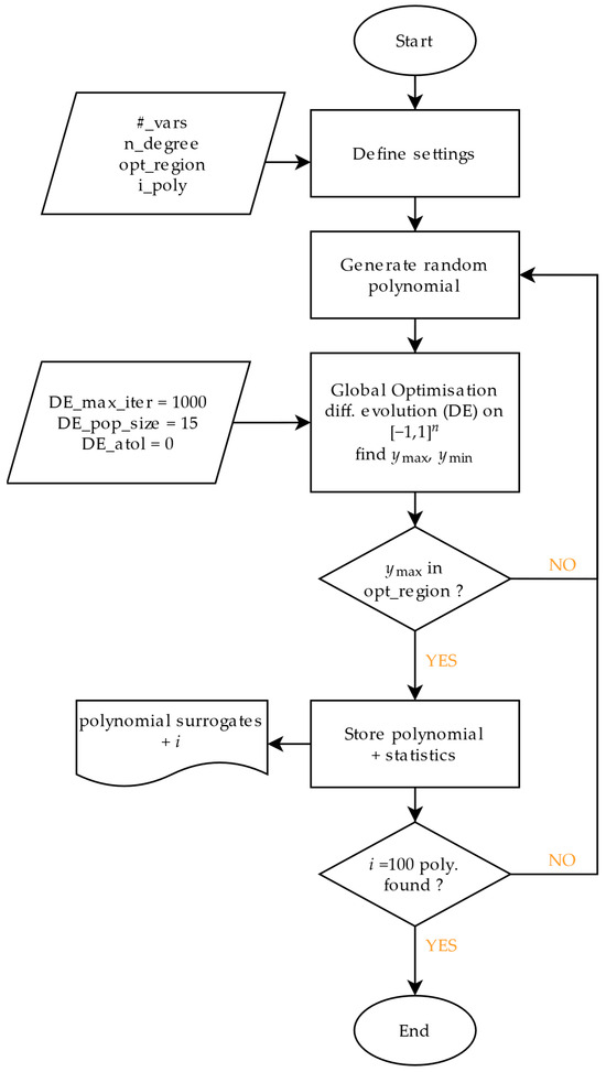
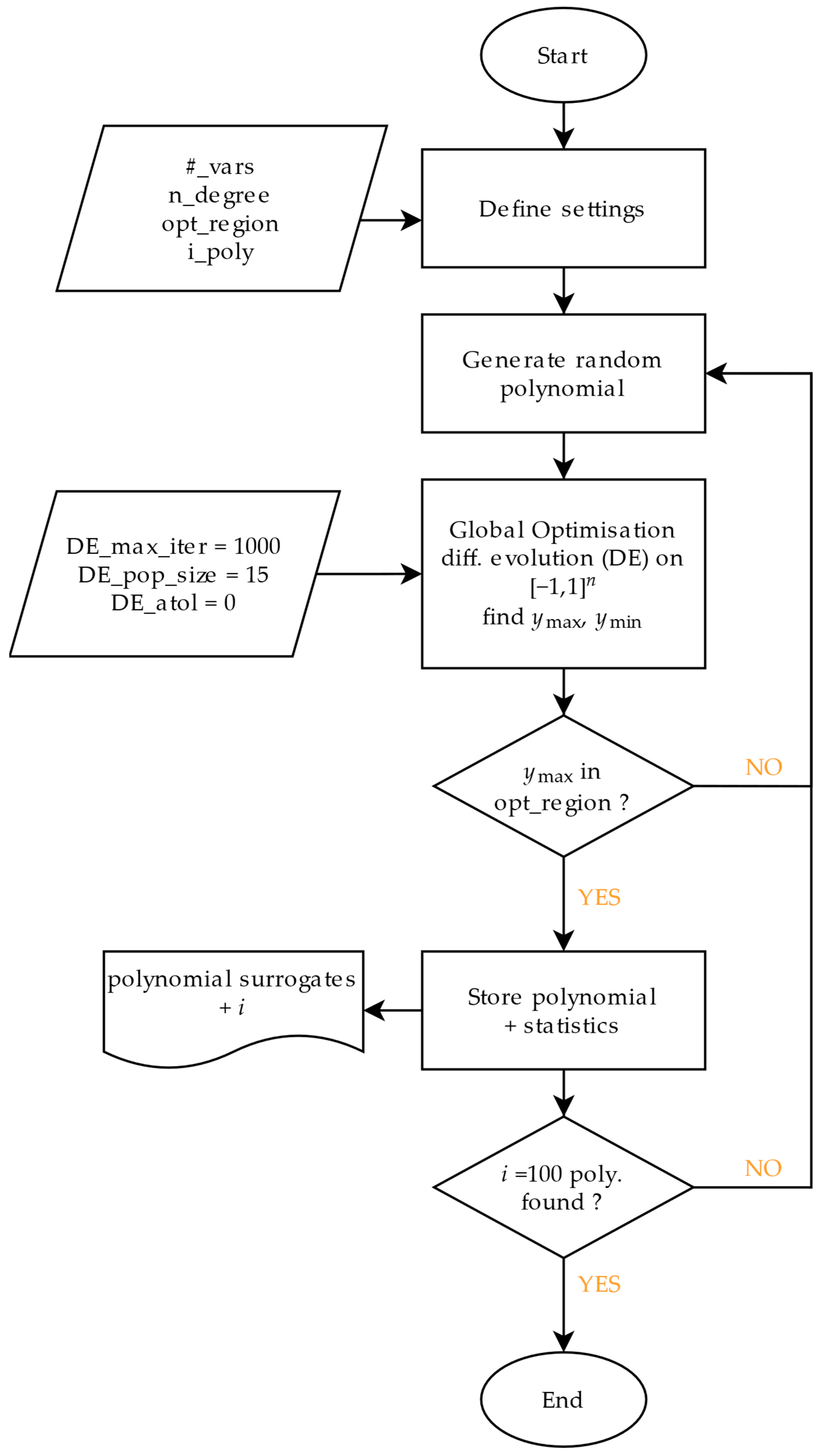
The polynomials are generated according to Figure 1. The mechanical process is characterised though knowledge that the user may have of the process. That includes the number of process parameters () to be modelled, represented by the number of variables in a polynomial function. In this study, the variable counts of three, five and seven are accounted for. It is argued that sampling these variable steps achieves a balance between coverage and tractability in practical experimental setups. Higher variable counts require substantially more sampling effort, typically exceeding what is practical for physical experiments. The provided evaluation allows insight into the behaviour of nearby variable steps, meaning that the results can be applied to similar modelling challenges without needing to fit the exact setup described in this work. Another characteristic is the complex behaviour of the process, which is expressed in polynomial degrees (). The polynomial behaviour of quadratic to quartic is taken into account in this work. This overlaps with the commonly used second degree response surface methodology (RSM) of DoE, broadening the complexity spectrum up to degree four and balancing the required sample effort needed to describe higher-complexity problems. Before modelling, the considered range of each process variable has to be defined, which here is polynomial variable With a priori knowledge, it should be foreseeable if the optimum of the process—so the best response—will be found at the edge of the range or in the middle. That is considered by having the optimum of the response with all the variables in the middle, so , or at the edges, so . Also, from preliminary test, the standard deviation of the process should be known. Consequently, a homoscedastic Gaussian noise factor is added. The surrogates are generated mostly randomly depending on the polynomial degree and variable count. Higher polynomials are partly constructed to have a saddle point or multiple optima to avoid similarities with functions of lower polynomial degree and to reduce computing time. In the next step, the generated function is tested for its optimum region within the bounds with a differential evolution algorithm and stored accordingly, e.g., for a quadratic polynomial with 3 variables. A fully defined quadratic polynomial with all terms is generated. The beta coefficients for all terms are randomly defined. Then, the location of the optimum is evaluated through an optimisation search. The polynomial is sampled with the specific sampling method and noise is added to the data. The process is repeated till 100 surrogates meeting the requirement of a quadratic polynomial with 3 variables and a specific optimum are found.
Figure 1.
Flowchart of the generation process of 100 polynomial surrogates to function as a process alternative for the comparison of sampling and ML modelling techniques.
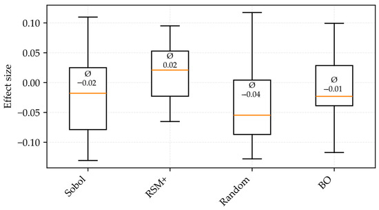
In preliminary tests, 100 and 1000 surrogates were tested for an identical variable setting of three variables, with third degree polynomials and 5% Gaussian noise added with a centred function optimum. The RMSE values of the models are compared to determine whether 100 polynomial surrogate functions are sufficient. Using a two-sided t-test, the RMSE values of the ML methods are compared individually for each sampling. The H0 hypotheses states that the mean RMSE values of both groups are equal. None achieves the significance threshold of p < 0.05; the lowest is p = 0.21, obtained for sobol sampling with the Generalised Additive Model (GAM). In addition, the Cohen’s d effect size is calculated with negligible practical differences as none reached the threshold of d > 0.2 (see Figure 2). Typically, values of d > 0.2, >0.5, and >0.8 are interpreted as small, medium, and large effects. As there is no indication for an effect or significance, the H0 hypothesis was not rejected, indicating 100 surrogate functions to be sufficient as sample size. These findings indicate that the generated polynomials for each setting show similar but not identical behaviour. It is therefore assumed that averaging the 100 polynomial surrogate functions results in a comparable model performance for each setting.
Figure 2.
Surrogate functions per setting. Evaluating the surrogate polynomials needed; effect size between 1000 and 100 functions for different sampling methods, none reaching the effect threshold of 0.2.
3.2. Sampling
In this section, general data handling is discussed and afterwards the different sampling methods are explained in detail. The entire sampling process is visualised in Appendix A Figure A1.
The number of training points for each polynomial surrogate function depends on and and is calculated through Formula (1). Two values are compared and the maximum is used as the number of samples needed for the specific polynomial function that is sampled. The first value is the binomial coefficient, which calculates the minimum terms needed to describe a polynomial function so that it defines the number of samples needed to describe the underlying problem. The second value is the sample calculation for a RSM, where defines the number of centre points of the star formation. RSM is used as a representative of the classical DoE hybrid sampling method, which is not flexible in terms of the number of samples to be taken.
With the necessary sample size calculated, the methods independently sample the surrogate models. Afterwards, the validation data can be randomly collected. The validation points are the number of training points increased fivefold to give a reliable comparison. The response for every sample is calculated and scaled from 0 to 10 to provide comparable RMSE values per variable combination. Only after that is the predefined Gaussian noise added, after Formula (2), to the y values of training and validation data, mimicking a real mechanical process. The values are evaluated for each individual surrogate polynomial using DE over the domain in the polynomial generation. They are used to scale the original for each sample point of one function to the range from 0 to 10. The error is a homoscedastic Gaussian noise, depending on the setting from 0 to 10%.
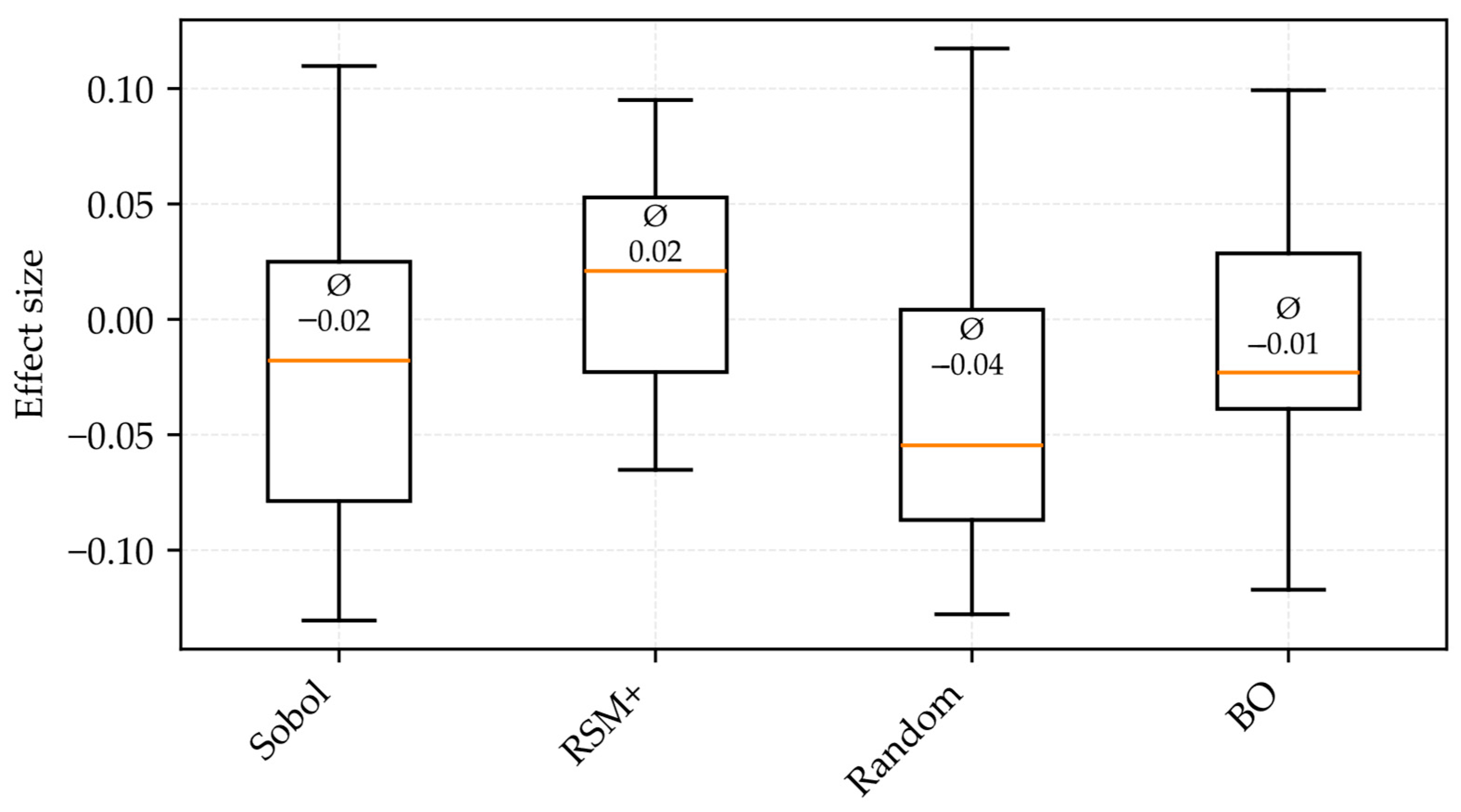
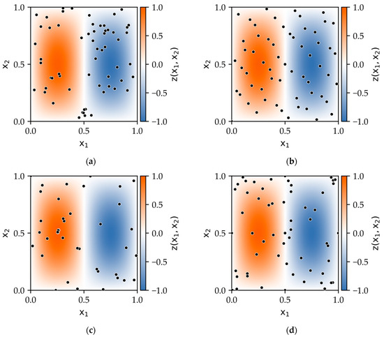
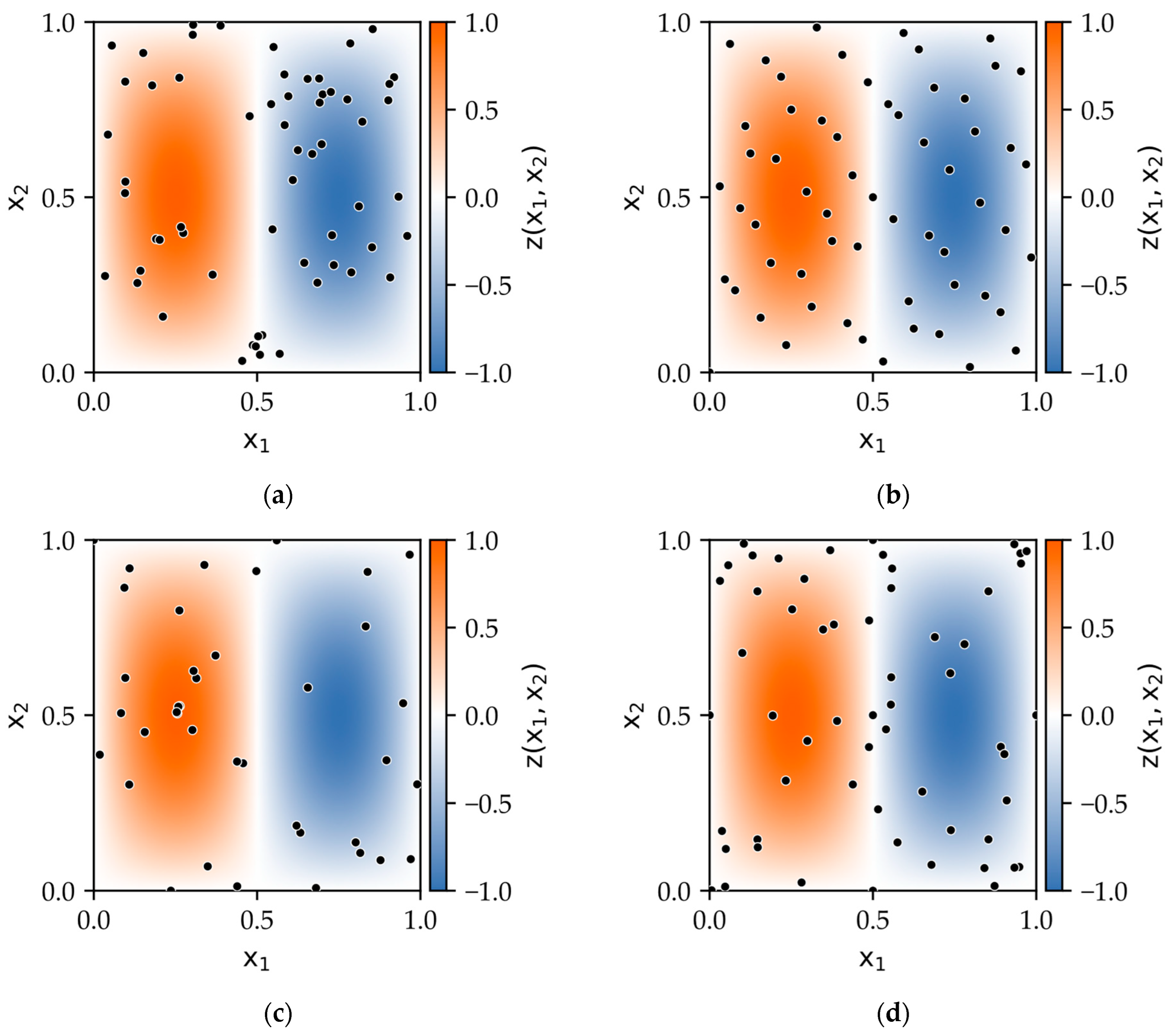
Random sampling is simple to apply as there is no fixed sample count or even distribution to be considered. It can also be applied sequentially but without having a learning effect through data generation. It can, however, cluster in regions (see Figure 3). It is widely applied and therefore considered as a reference.
Figure 3.
Illustrative sampling distribution of 60 samples on an exemplary wave function for an intuitive visual comparison of sampling behaviour. (a) Random sampling (clustered). (b) Sobol sampling (space filling). (c) Bayesian optimisation (sampling converges to optimum). (d) RSM+ (ordinary CCI points with exemplary G-Optimal additional points).
Space filling sampling has its origin in computer experiments, as common linear regression methods for physical experiments were not suited for non-linear dependencies, inexpensive tests or large experimental regions [17]. LHD and its further development, MaxPro Designs, are the best known adopters of this challenge [24]. The goal is to achieve a more space-filling design than random sampling. In the recent literature, Sobol Sampling has advantages over LHD [25,26] and at least one of its configurations [27]. Sobol sampling is based on a (t; s)-sequence in base 2 and constructs its points deterministically so that each new point reduces gaps and clustering in the experimental design [28]. For dimension d, the sample point is generated according to Formula (3). Here, S denotes the sample index, ⨁ is the bitwise XOR operation, is the binary digit of S at position k, m represents the number of binary digits used to express S, and the direction numbers .
Adaptive sampling introduces the idea of taking samples iteratively instead of defining the test scope a priori. It is therefore used to learn from the already taken samples and either directly suggest optimised parameters like in an optimisation algorithm [29] or build an active learning model [30]. In this case, BO with Gaussian Process Regression (GP) as a surrogate model is used. Starting with a subgroup of five samples, a GP model is built with a radial basis function (RBF) kernel. The expected improvement over the experimental space is iteratively calculated till is reached. It therefore behaves like an optimisation algorithm, only trying to optimise the response rather than the GP accuracy globally.
The representative for Classical DoE sampling is a hybrid of a central composite inscribed (CCI) design and G-Optimal design. As mentioned in Formula (1), RSM provides a fixed number of sample points depending on the . It is designed with corner points and a star formation with centre points. The centre points are repeatedly tested to indicate variance of the process. The combination of star and corner points allows the modelling of quadratic effects [31]. As a disadvantage, there is no typical adjustment for CCI modelling for a higher complexity than second-order polynomials. To adapt for that discrepancy, when more sample points for higher polynomials are needed, additional points are generated with another DoE method: the G-Optimal design. The combination is subsequently referred to as RSM+. It minimises the maximum prediction variance across the entire design space after Formula (4). denotes a design point in the n-dimensional design space. The function denotes the polynomial basis vector at x (e.g., for polynomial regression). The design matrix is denoted by X and is the inverse of the information matrix.
The code generates 700 reference points randomly in the design space. At the beginning, a differential evolution algorithm distributes the missing sample points randomly. The position of the added augmentation points is iteratively updated with the G-criterion in Formula (4) as the optimisation function. The goal is to minimise the maximum prediction variance across the reference points.
G-Optimal design was preferred to other optimal designs (e.g., I-Optimal or D-Optimal). D-Optimal was disregarded as it focuses on parameter estimation precision and not global modelling [18]. I-Optimal was rejected as the prediction robustness in case of the given complexity, and multidimension of the design space was prioritised over average performance, including the risk of regions with high variance.
3.3. Modelling Process
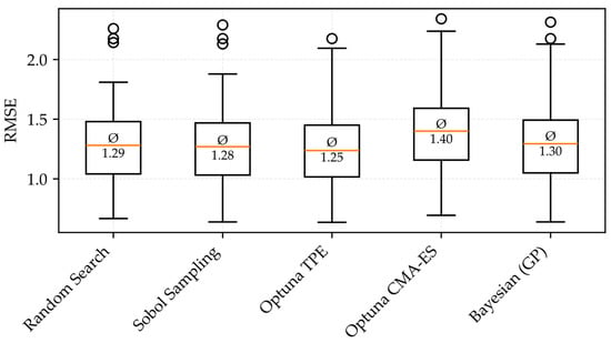
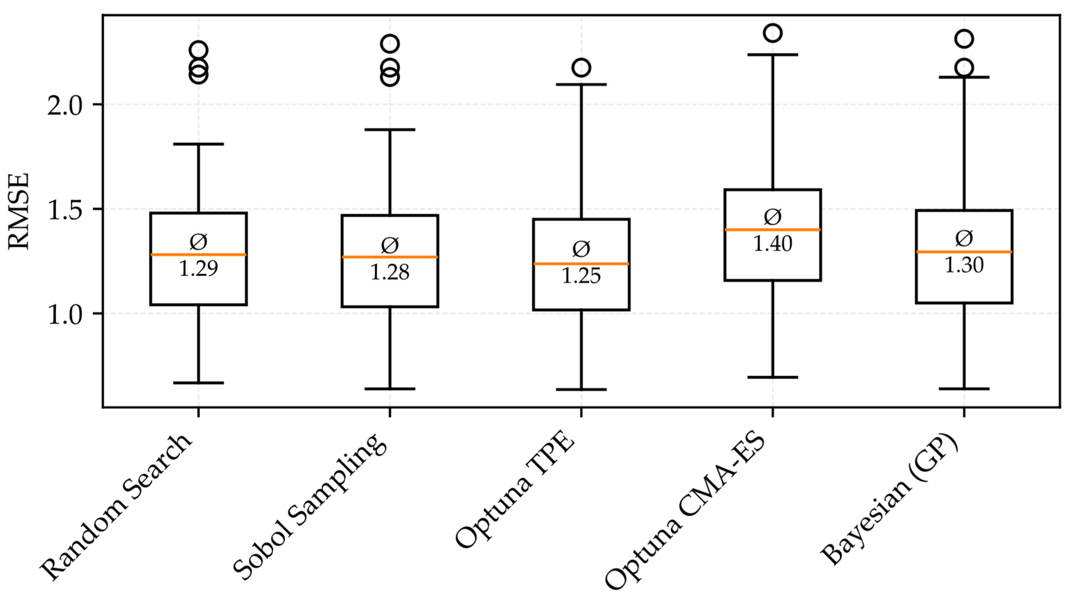
The procedure for the regression is standardised and visualised with the ML method random forest as an example in Appendix A Figure A2. The pipeline starts by defining the machine learning specific hyperparameters (HP) to be improved (see Appendix A Table A1). The aim was to select the most significant ones, but this cannot be guaranteed without a separate analysis. For each HP, a range was set which was used for optimisation. The optimisation problem was solved with the Optuna framework, and specifically one of the most common used: the tree-structured parzen estimator (TPE) Sampler [32,33]. TPE models the HP search space using two density estimators: with the density of the best objective values and for the density of the remaining configurations. New sampling points are generated by sampling from and selecting those that maximise the ratio of the two Gaussian Mixture Models . The procedure is proportional to the expected improvement criterion used in BO, since the approach searches for an optimum rather than an overall model accuracy. Optuna’s TPE Sampler has the advantage that it is theoretically more sample-efficient than random or space-filling (like grid or Sobol) as it explores optimum regions rather than sampling the HP space uniformly. Other advanced optimisers, e.g., BO, are promising but not used as the TPE sampler has a constant-liar parallelization feature which improves practical scalability. Without custom handling, optimisation algorithms like Particle Swarm Optimisation cannot natively handle categorical or log-scale search spaces, which excludes them from further evaluations. To make a more informed choice, various HP optimisation methods were tested using LightGBM, an ML method, as an example (see Figure 4). The HP of these methods and LightGBM are shown in Appendix A Table A2. Random sampling was used as a benchmark for comparison. Grid search was replaced with another space-filling method, namely Sobol sampling, which can adapt to the limited number of data points that grid search cannot. CMA-ES is another method from the Optuna framework, but it requires custom handling of categorical data. BO with Gaussian Process as a surrogate was used for the final comparison. A total of 100 functions with three variables, third-degree polynomials, 5% Gaussian noise and a centrally located optimum, were chosen. The training data were sampled using Sobol sampling. Optuna TPE is considered a robust performer that delivers the best results with the fewest outliers. The difference in absolute value is limited. This is most likely because the added process noise has become the limiting factor for the model and therefore the optimiser’s performance. However, this assumes that the LightGBM model is not robust to changes in hyperparameters for this process. As LightGBM is tree-based, its leaf-wise tree growth makes it sensitive to tree-complexity parameters, providing no evidence for a hyperparameter-independent model. In this test setup, random search provided acceptable results and would have been chosen if computational speed had been prioritised. While it is not possible to make a generalised statement about the scope of the entire test, the selection of the Optuna TPE sampler is nevertheless justified based on the indication that it produces the most accurate models in this comparison.
Figure 4.
Comparing different hyperparameter optimisers with the RMSE value of the ML model LightGBM being optimised. Optuna TPE delivers the best result and is used for further analysis.
The TPE Sampler is used in several trials to optimize the HP. In each trial, the training data is split into 5 folds for cross-validation. The average RMSE value is calculated and serves as a response for the adjusted HP in that specific trial. The best HP results are saved and the whole training dataset is used to train the final model. The RMSE value of the model compared with the validation dataset is saved as a result. This is repeated for all surrogate functions of every sampling method and every ML method, which are described in the following section.
3.4. Machine Learning Methods and Evaluation Parameters
ML methods are classified depending on different characteristics, e.g., using all or mainly nearby data points for prediction, whether model complexity is data adaptive or fixed, and whether smooth or abrupt prediction changes appear. The following taxonomy and the corresponding behaviour descriptions are loosely based on Hastie et al. [34].
Global parametric smooth models use all available training data to estimate a predefined set of parameters by minimising a global error function, usually ordinary least squares. Nearby inputs produce nearby outputs, which leads to a smooth prediction surface. Some of the examples used regularise coefficient magnitude or suppress parameters to better fit the data. The used examples are linear regression (LinR), polynomial regression of degrees 2 to 6 (Poly2-6), L1 + L2 regularised polynomial regression of degrees 2 to 6 (Poly_reg2-6), and Elastic Net (E-Net).
Global additive basis-function models expand the prediction function with multiple basis functions to describe the data with non-linear relationships. Examples used are GAM and Multivariate Adaptive Regression Splines (MARS/EARTH).
Kernel methods use similarity relationships between observations defined by kernel functions. The output is influenced by decreasing strength by nearby datapoints. This results in continuous and typically smooth prediction surface. Models considered are support vector regression (SVR), Gaussian process regression (GP) and Kernel Ridge Regressor (KRR).
Local instance-based methods concentrate their predictions on an average of the nearby observation in the feature space. This produces strong local behaviour with distant observations having no effect on the current prediction. In this work, k-nearest neighbours (kNNs) are used.
Tree-based partition and model tree methods subdivide the feature space through rules-based nodes into regions. The result is a piecewise constant or locally regressed model that is highly interpretable through the rules it uses to divide terminal regions. Representatives are Decision Tree (DT) and Cubist.
Tree Ensembles: Bagging trains multiple tree-based models on subsets of the training data. By averaging the models’ response, the individual error and variance are reduced. Common models are random forest (RF), M5Prime Model Tree bagging (M5P_bag) and Extra Tree Regression (ExTr).
Tree Ensembles: Gradient Boosting sequentially trains tree models. Each iteration weighs the training data so that the previous prediction error of the ensemble can be focused on. The final response is the weighted combination of all trees. Examples are CatBoost (CatB) and Light Gradient Boosting Machine (LightGBM).
Neural networks are networks of interconnected nodes usually organised in layers. Each node uses an activation function to calculate the output depending on the weighted sum of the inputs and a bias. The summed result is compared with the given training sample. Through back propagation, the connection weight of each input of each neuron is adjusted to improve prediction accuracy. A basic representative is the multi-layer perceptron (MLP).
With the polynomial functions, regression variable interaction is modelled up to a polynomial degree of four. However, in our modelling pipeline, only the polynomial regressors are basis-restricted. Most ML models, such as kernel, local instance, tree-based and MLP models, can implicitly represent interactions of arbitrary order. In a real-world application, these non-parametric models can capture higher-order dependencies.
Model performance is evaluated with RMSE. RMSE measures prediction error by averaging the squared distance between predicted and observed target values. Due to its squared properties, it is sensitive to outliers. It is favoured over alternatives because it presents the results on the same scale and in the same units as the training data. This aligns with the aim of this research: to make the results accessible to non-domain experts. Furthermore, it makes the detection of overfitted models easier by highlighting mismatches between regression and validation data through its squared properties. Alongside the RMSE outlier handling explained in Chapter 4, it therefore helps ensure that conclusions are not influenced by overfitted models. One of its downsides is that it is not scale-invariant, so the results are not directly comparable across datasets. Therefore, additional z-standardisation is used, which will be described in detail in the next section.
4. Comparison of the Results
This section outlines the various steps involved in preparing and evaluating the data for creating diagrams and tables. Appendix B Figure A3 provides an overview of the process.
Two separate evaluation workflows have been set up, as they perform better in different quality metrics. The main difference between them is how they handle outliers. In the first workflow, outliers are removed from the entire dataset using the 3xIQR method. For each setting (4 sampling, 54 polynomial and 26 ML), outliers are defined and removed using the 3xIQR rule. This eliminates extreme RMSE values that probably occur through failed convergence. A Spearman sensitivity check is performed on the entire settings vector to evaluate whether the removed outliers alter the overall ranking of the ML methods. With a Spearman value of , the dataset appears to be compromised, with indicating that the predicted alteration is statistically significant. The majority of the observed RMSE values are in the lower single digits. The removed outliers are far beyond this range. The mean RMSE change from to indicates that the extreme RMSE values are eliminated and therefore the Spearman analysis correctly indicates that the ranks correlate to a noticeably lower extent. Alternatively, the outlier handling is performed through a 1% two-sided winsorisation, which caps the extreme values at the 1st and 99th percentile. Here, the Spearman rank correlation indicates a value of for the ML methods, with , indicating a robust changed dataset. The mean RMSE value drops to , which is still interpreted as high, as the polynomials are scaled from 0 to 10 such that a high mean difference indicates misfitting of the regression methods. The winsorised dataset is evaluated further, as it does not alter the rank correlation after Spearman. A log transformation is applied to both variants, as RMSE values are typically right-skewed. The aim is to achieve a more stable objective for further grouping and comparison by compressing the remaining large values. The 3x IQR model has a marginal , whereas the winsorised model has a marginal . The metric shows how much of the variance of the data can be explained by the model. In this case, the removal of the outliers favours the model metric, which is typically interpreted as a better result. Nevertheless, 30–40% of the variance could not be explained. Other reasons may be the higher order interactions or the influence of the hyperparameter tuning.
A linear mixed model is built on the winsorised results to quantify effect sizes of the test setup. The complexity of the linear mixed model is evaluated using linear, quadratic and cubic effects with 5-fold cross validation. The trained log(1 + RMSE) value is calculated and compared with the held-out log(1 + RMSE) value for each fold. This is repeated for each of the three models. The average values for the five folds are presented in Table 1.
Table 1.
Robustness check through 5 cross-fold different linear mixed model complexities. Average RMSE value of the 5 folds for the trained and validated test data.
According to the test, the cubic model does not improve generalisation as the model performance deteriorates. This suggests that a quadratic linear mixed model is adequate for demonstrating the effect size. Higher-order models were not considered as they do not provide additional predictive benefit and reduce interpretability. The final chosen model formula is presented through Formula (5).
This model estimates the fixed effect coefficients of the variables and their two-way interactions and accounts with the random intercept for the possibility that the 100 different generated polynomials may have their own influence on RMSE. With the intercept, each polynomial gets its own baseline difficulty even if generated with the same characteristics. The polynomial settings are defined through the 54 levels of number of variables, polynomial degree, location of the optimum and added noise.
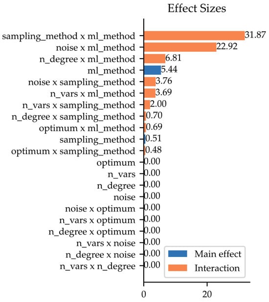
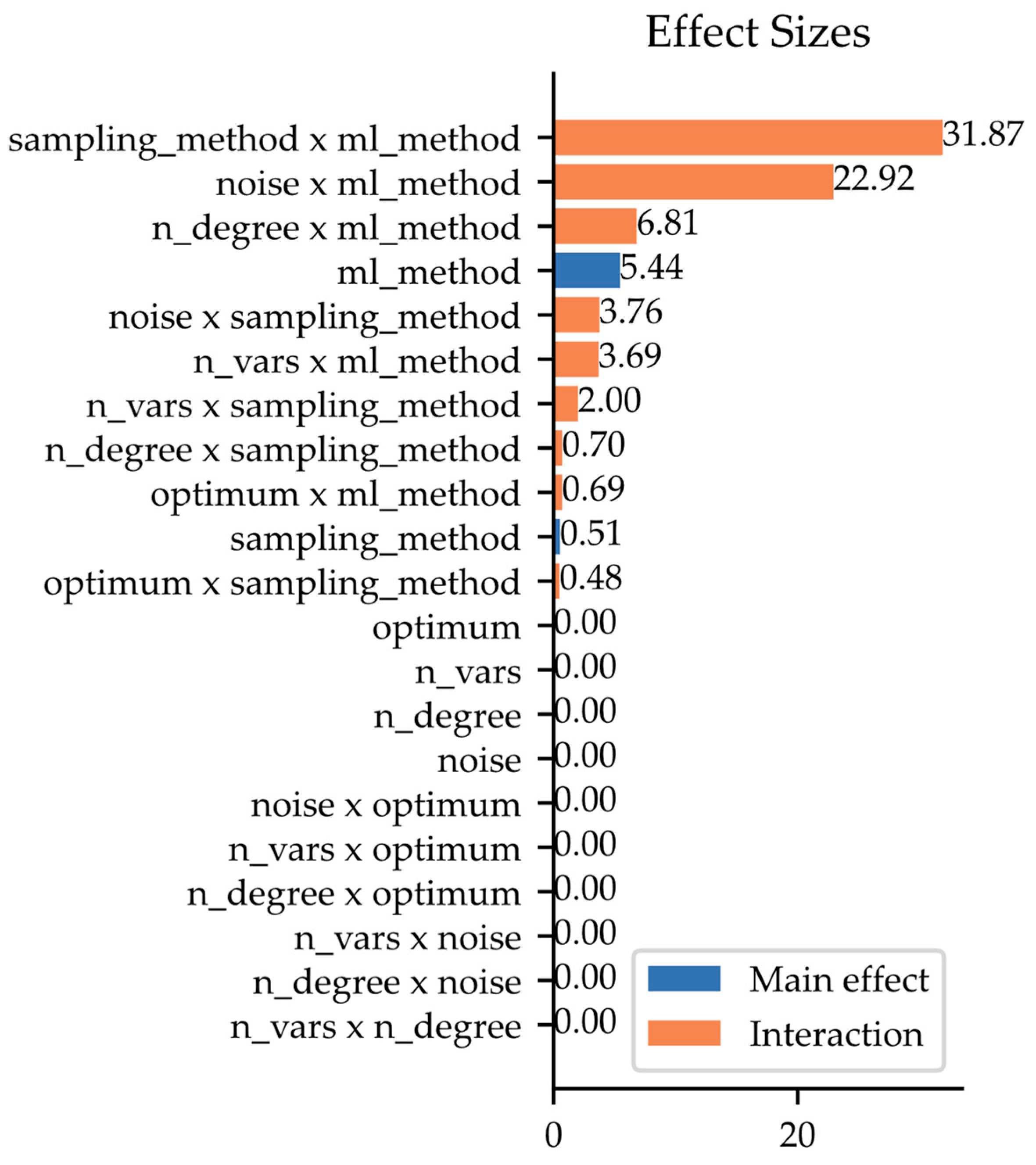
Figure 5 shows the values that approximate effect-sizes derived from the Wald test statistic of the winsorised linear mixed model. Visualisation is used to rank the experimental factors and interactions according to their contribution to the RMSE result. The contribution is calculated after Formula (6).
where is the Wald statistic for that term, and is the residual degree of freedom of the fitted linear mixed model. They reflect the relative strength of each term under the linear mixed model to provide a comparable measure of term importance.
Figure 5.
Calculated effect size with Wald statistics for the top 21 most influencing variables according to the winsored linear mixed model.
Here, the RMSE value is shown to be heavily dependent on the combination of sampling method and ML method. Overall, the main effects are relatively small; only the choice of the ML matters. Interactions, especially noise and the ML method, are important. All effect sizes are classified as significant when measured with Wald test and p-value. This is a known behaviour of large sample size, resulting in high statistical power. With high statistical power, metrics like p-values or pairwise t-tests do not generate additional information gain as they tend to produce lower values.
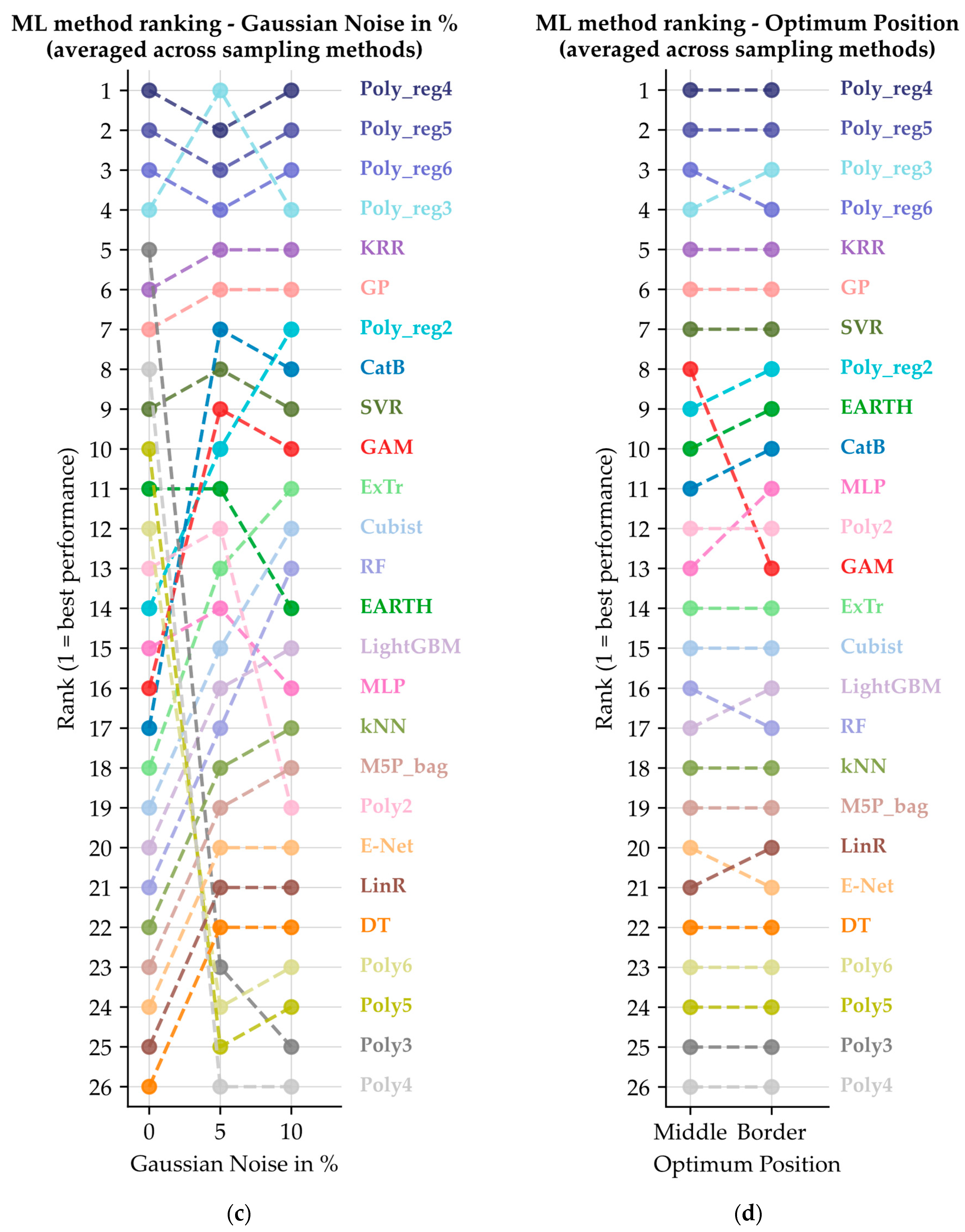
The biggest difference to the 3xIQR model is the high effect size of the interaction between sampling and the ML method, which is reduced to semi-partial , with the ML method moving to the second highest effect size of . When the estimated coefficients of both models are compared, it can be seen that the winsorised model is heavily influenced by the Poly2-6 regressions (see Table 2). Excluding these regressions from the mixed linear model makes the effect sizes of the winsorised and 3xIQR models comparable, with the interaction between noise and the ML method dominating. To put this into context, higher-degree polynomials are useful for describing lower-degree polynomial surrogates, but perform worst with noisy data (see Appendix B Figure A6c). As noise is such an important variable, a mixed linear model that overfocuses on the performance of Poly2-6 is not used for further analysis.
Table 2.
Top 5 coefficient values, model dependent.
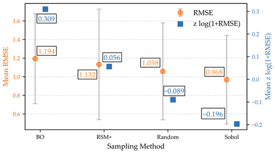
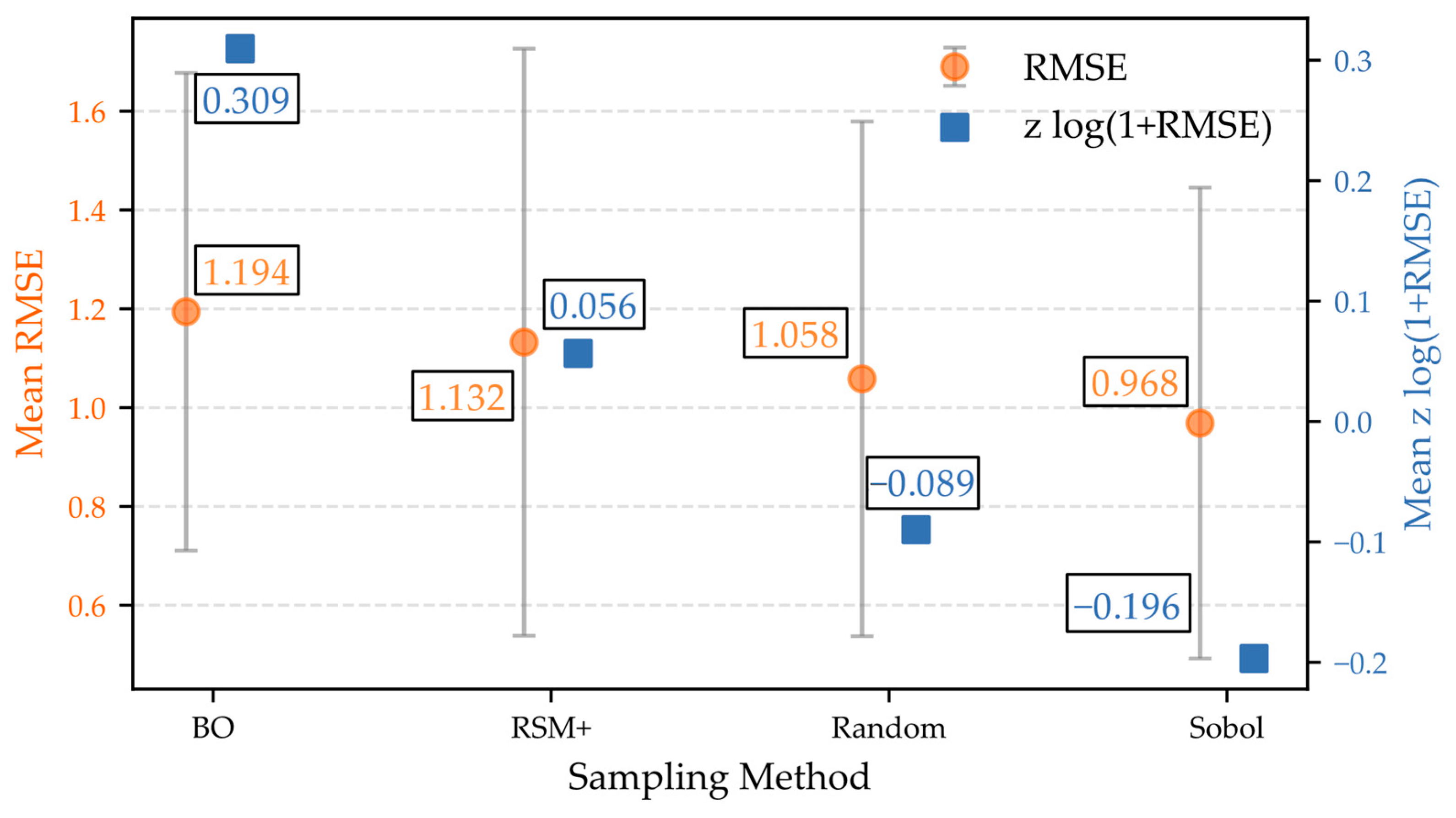
The following evaluation is based on the removal of outliers. Figure 6 shows the mean RMSE values and standard deviation of the sampling methods. This provides a practical representation of the RMSE values and their behaviour on the original scale. The standard deviation is quite high, as the sampling method has a minor effect on the overall value, and other influences, such as the ML method, generate a high degree of deviation. On the other hand, the graph shows a value that accounts for the right-skewed behaviour of the RMSE values, which are not normally distributed, with log(1 + RMSE). Additionally, the influence of the ML methods are accounted for through z-standardisation of every ML method. For the value of the second, more sufficient evaluation is no longer practically interpretable, so both are plotted.
Figure 6.
Comparing the mean RMSE and mean z log(1 + RMSE) values for each of the applied sampling methods, averaging over polynomial surrogate settings and ML methods.
Statistically, the values below zero indicate a better performance than the group average. For both, lower values indicate a better model fit and, in this case, a better sampling method. Sobol performs best, and random sampling outperforms RSM+ and BO. This suggests that exploratory sampling strategies like Sobol and random outperform the partly structured and optimum searching approaches considered here.
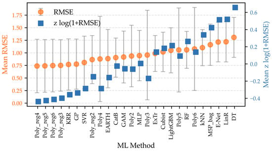
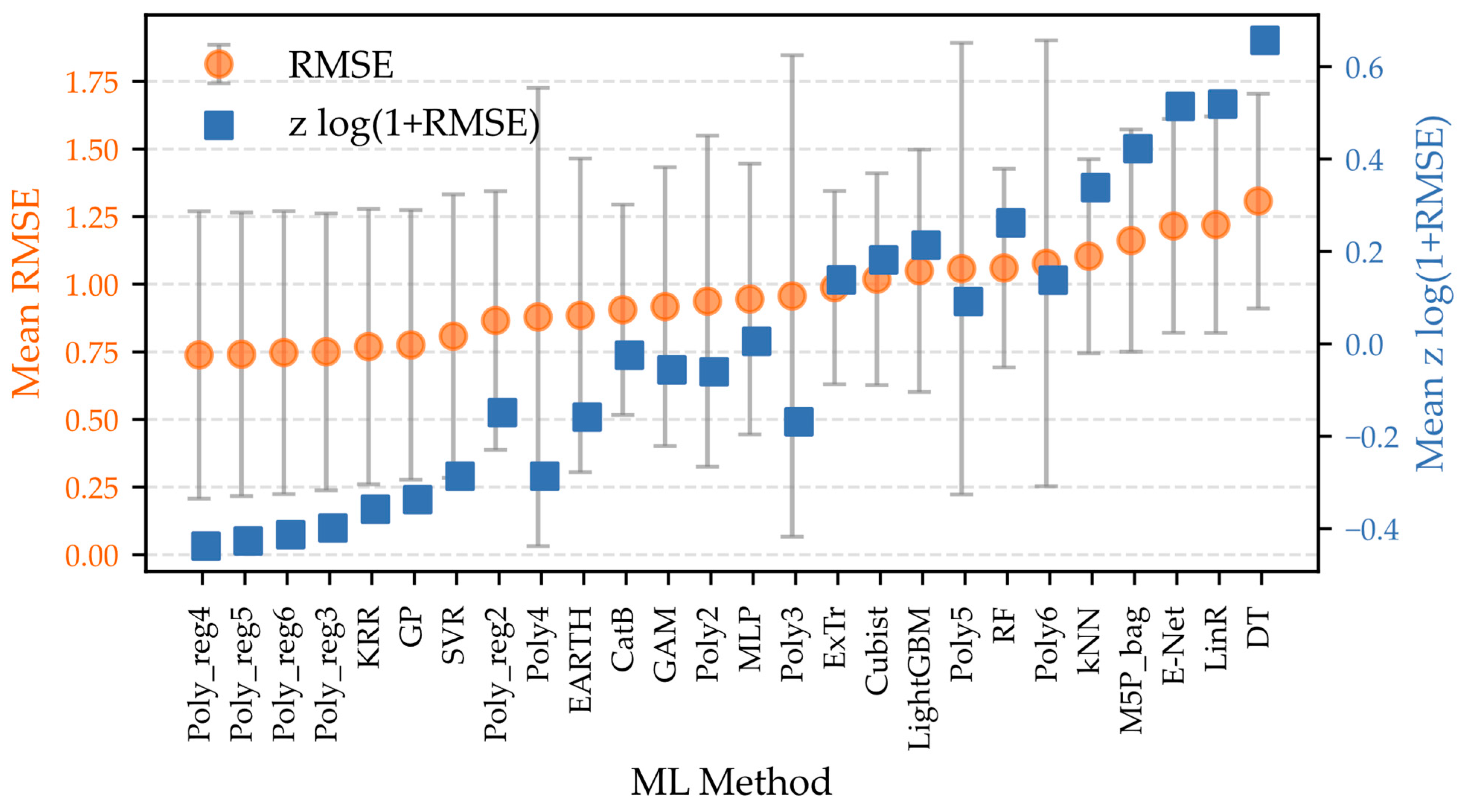
The next evaluation setup evaluates the ML methods in the same way and accounts for the different behaviours of the sampling methods. Figure 7 shows the sorted ML methods, highlighting the superior performance of the regularised polynomials. Overall, the influenced range of the mean z log(1 + RMSE) is larger than that of the sampling methods, which again demonstrates the greater effect of ML methods compared to sampling methods. The best models were the regularised polynomials, especially when combined with Sobol sampling, as shown in Appendix B Figure A4. It is assumed that Poly_reg4 dominates as it uses the same structure as the underlying surrogate polynomials, handles noisy data through its regularising terms, and does not overfit as Poly_reg5 does for the polynomial surrogates with degrees 3 and 4. An additional advantage of regularised polynomial modelling is the potential to handle collinearity in the data, even if this was not intentionally researched in this study [9]. Kernel-based methods follow closely behind.
Figure 7.
Comparing the mean RMSE and mean z log(1 + RMSE) values for each of the applied ML methods, averaging over all polynomial surrogate settings and sampling methods.
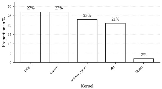
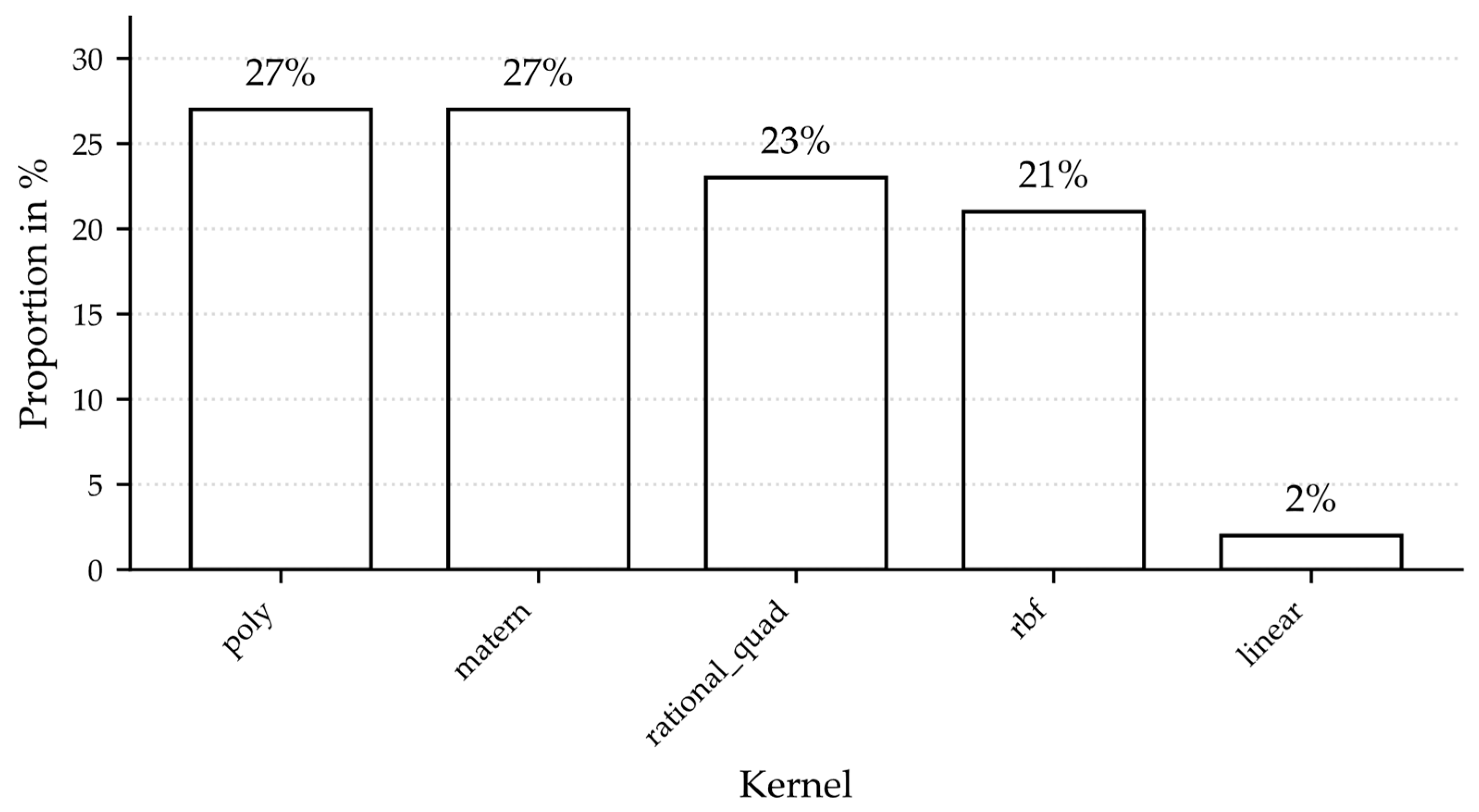
As kernel methods behave fundamentally differently depending on the kernel distribution, Figure 8 shows the distribution of the kernels. It is shown that not only polynomial kernels were used to describe the polynomial surrogates. This calls into question the validity of the thesis that the Poly_reg3-4 only perform well because they are similar to the surrogate. The fact that kernel methods perform well using a variety of kernels indicates that the regression performance of Poly_reg3-5 may be heavily dependent on similarity to surrogate models, but not solely so. Global additive basis-function models perform better than the neural network. The tree models tend to perform badly, except CatB.
Figure 8.
Distribution of the kernels used through the Optuna TPE hyperparameter optimiser for all kernel methods: SVR, GP and KRR.
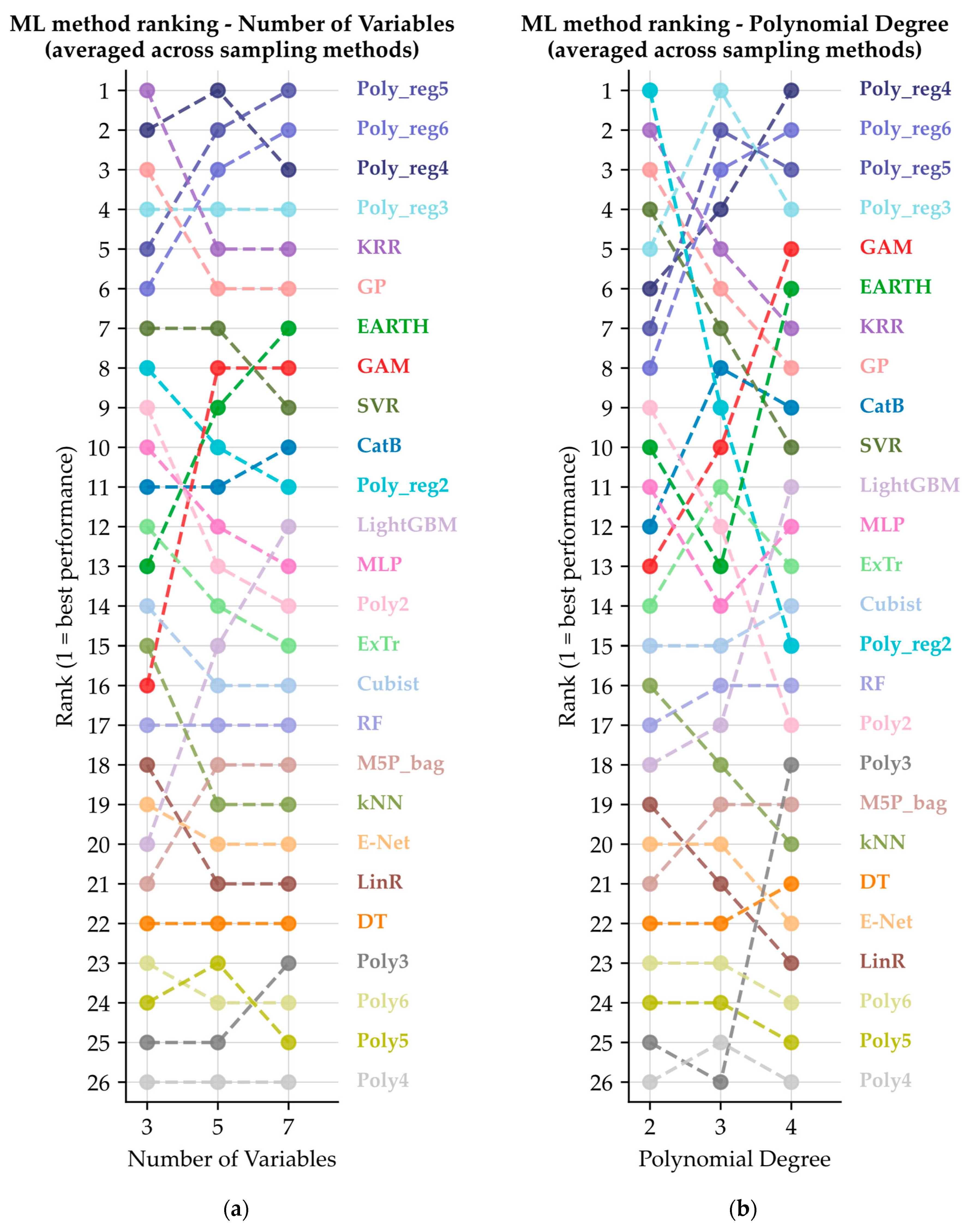
Additionally, the performance of the sampling and ML methods for each variable step was analysed (see Appendix B Figure A6). Essential take-aways are the effect ranges and optimum direction. On average, the RMSE value declines with higher . This behaviour should depend primarily on the number of samples, which was set relative to the complexity of the polynomial and is therefore ruled out. Other possibilities are a missing random variable or the effect of 3xIQR removal of high values, which may occur more frequently on higher-dimensional polynomials. For and , RSM+ changes performance at higher levels. This may be due to the dominance of the G-Optimal sampling points for higher sampling counts. Overall, and the location of the optimum have a minor effect on the performance. However, the optimum tends to worsen when it is in the middle of the search space. This can be illustrated using a second-degree polynomial as an example. If the parabola has its optimum in the middle, a turning point must be modelled, which is much more complicated for linear regressions than following the gradient upwards. A larger deviation between the regression and the data occurs when the optimum is in the middle of the modelled space. For optimums on the border, the difference is only significant after the turning point.
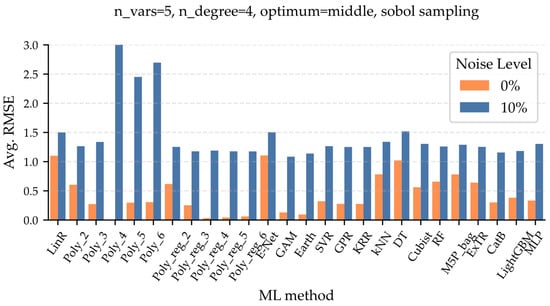
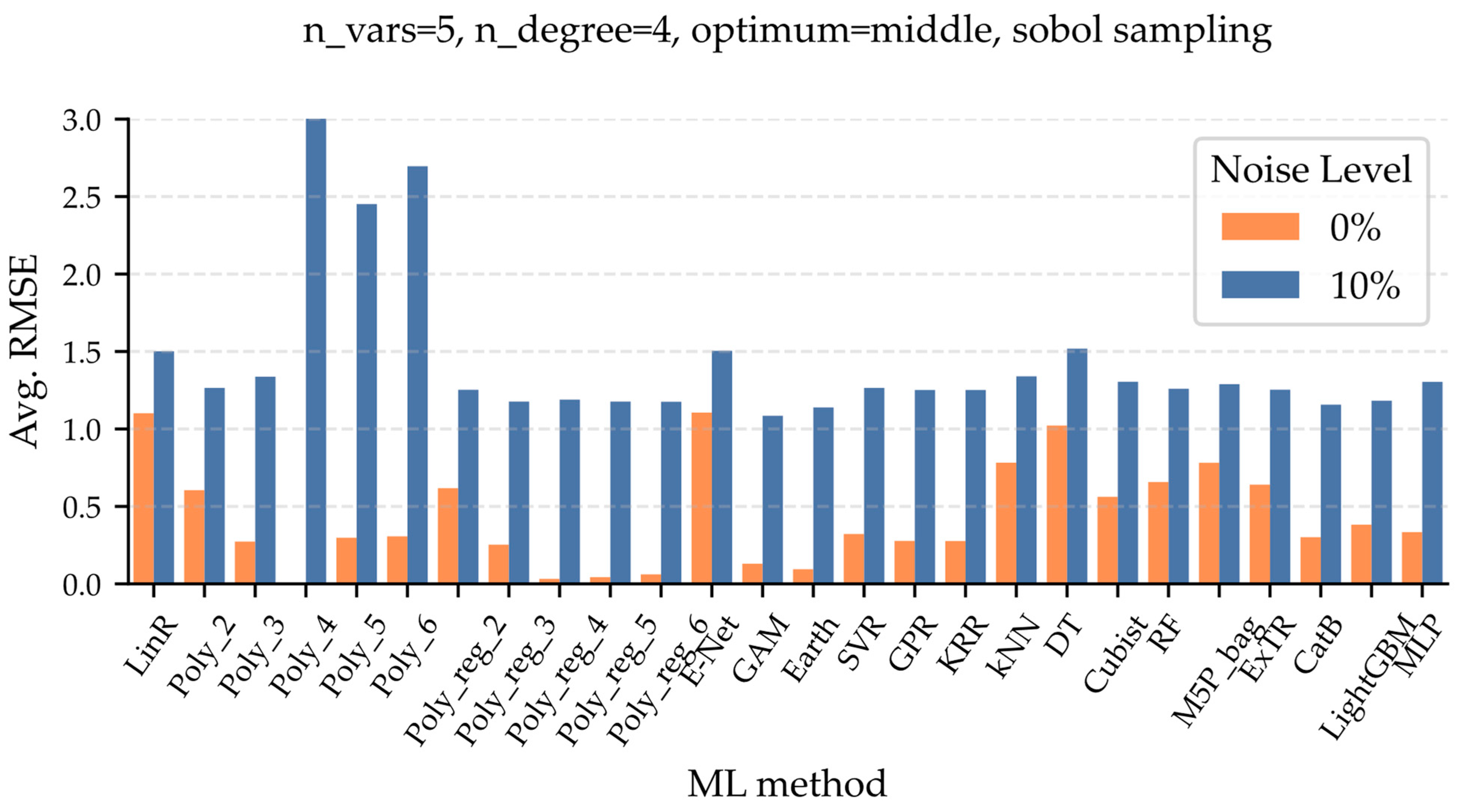
As previously mentioned, the added Gaussian noise is the most influential variable. The difference in performance can be seen in Figure 9. It shows the mean RMSE values of the polynomial surrogates with , and centred optimum with Sobol sampling. The noise varies from 0% to 10% of the polynomial y scale. Remarkably, the performance of the ML methods evens out. This may be due to the noise threshold, beyond which no method can perform better. Similar behaviour concerning the averaged results during noisy behaviour and high RMSE values for polynomial regression can be observed in physical experiments [35].
Figure 9.
Exemplary results of the RMSE value for one polynomial surrogate setting for each ML method depending on the noise level, showcasing the averaging effect through the noise level.
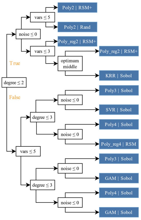
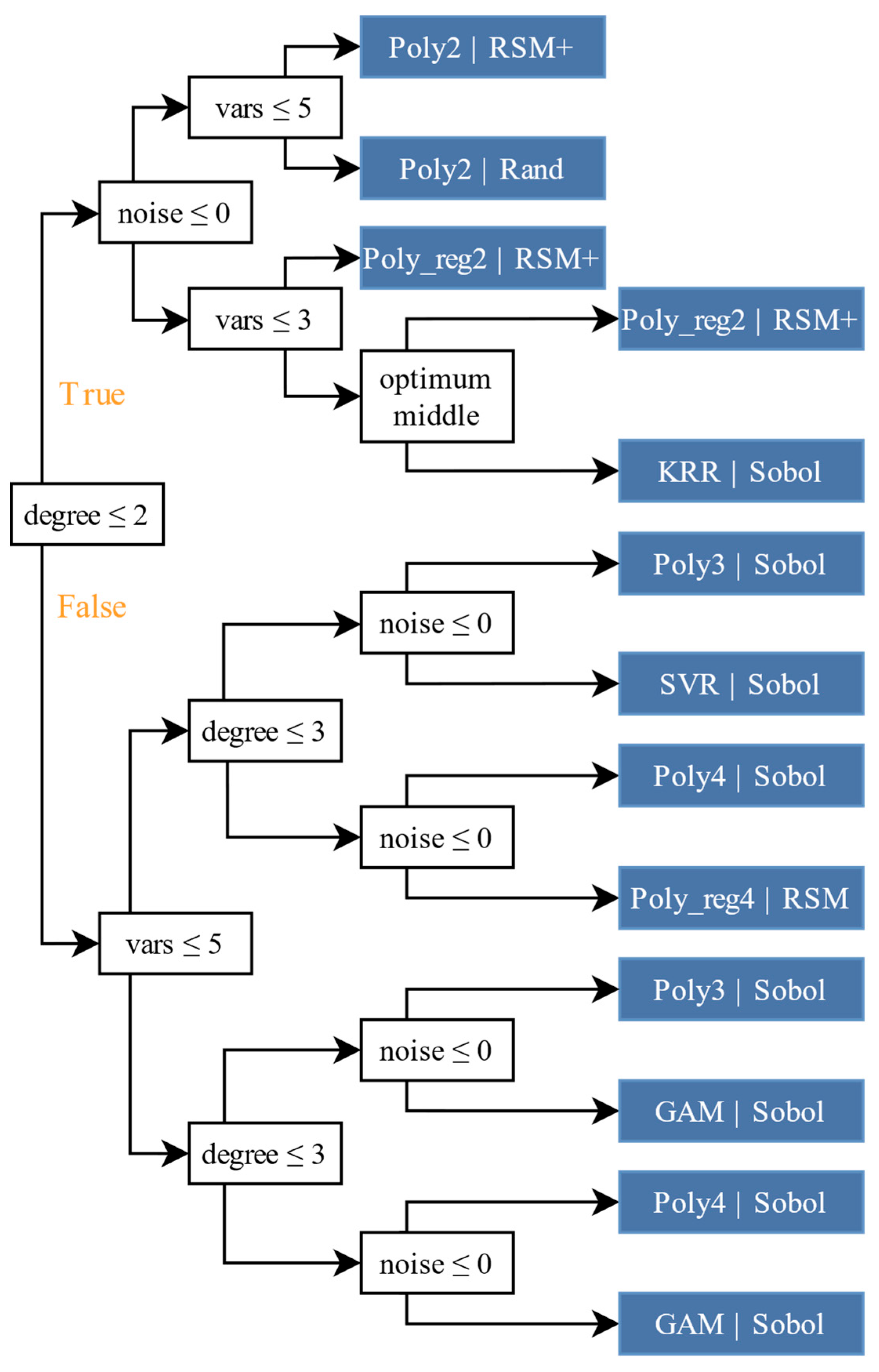
5. Cheat Sheet–Tree-Based Meta Model
It was noted at the outset that users wishing to model a process likely have little understanding of the advantages and disadvantages of ML and sampling methods. This highlights the need to provide users with a clear guide to help them select an appropriate combination based on their existing prior knowledge of the process they want to model or optimise. In this section, a tree model with beam search is therefore generated. The beam search recommendation tree was chosen because it evaluates multiple split possibilities and their future subtree quality before selecting the most promising one. Based on the 3xIQR RMSE results, the average RMSE value is calculated for each surrogate variable setting and for each combination of ML and sampling method. Thus, for each of the 54 settings, 104 combinations are ranked. The beam search suggests regions of the tree in which the leaf scores calculated using Formula (7) must be minimised.
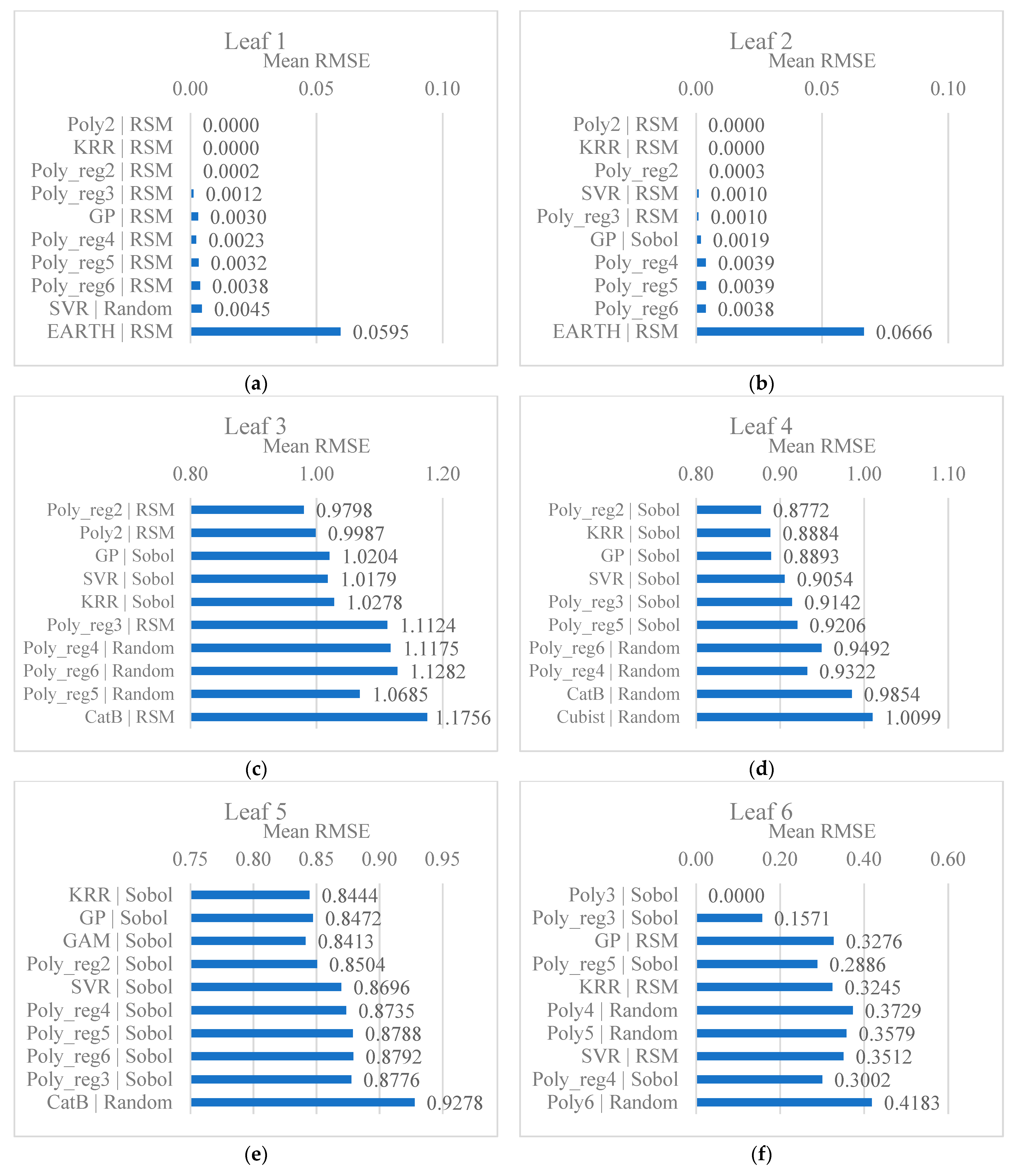
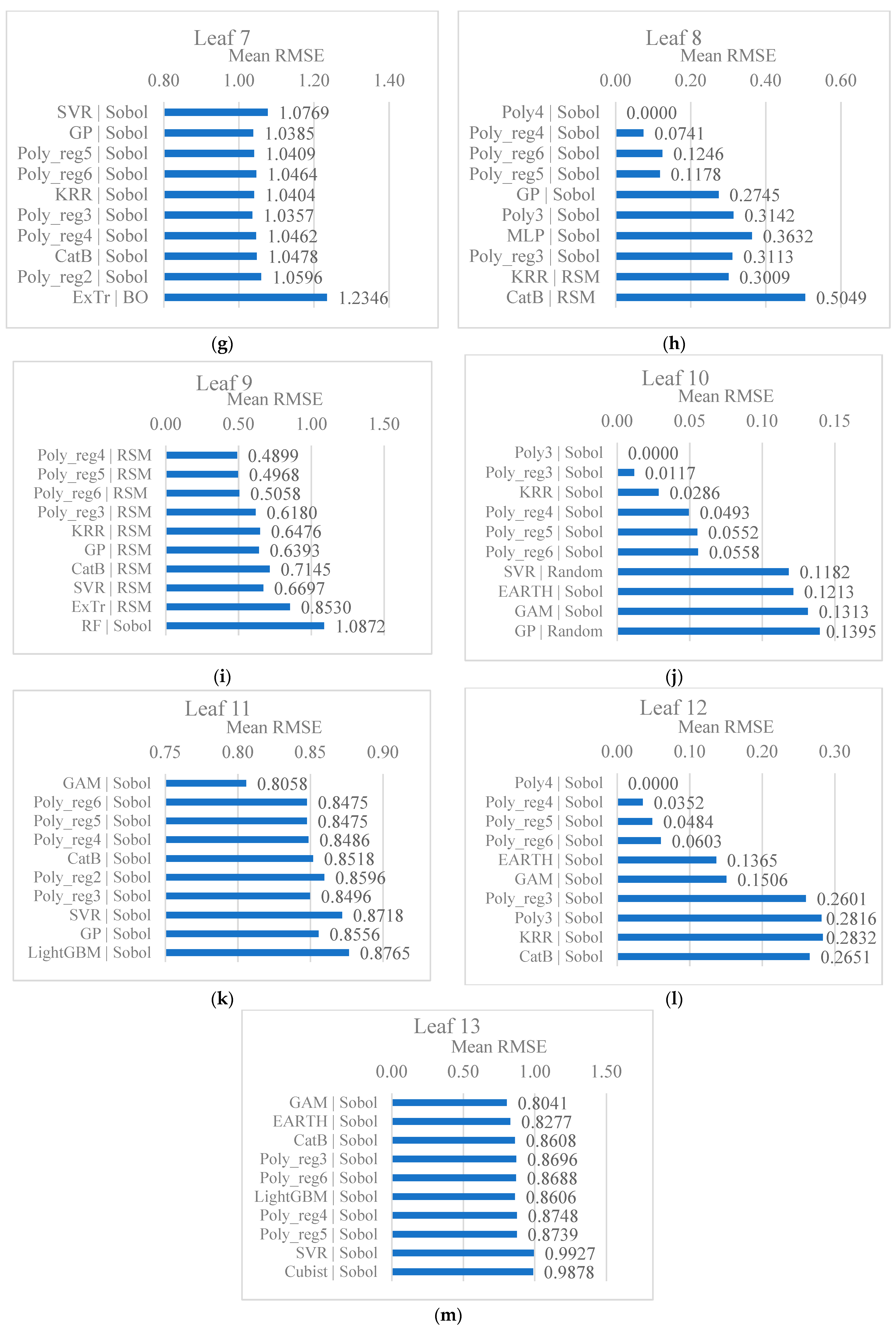
For a given leaf with K settings, the average rank and stable performance of each ML method are calculated through the average rank and its variance . The five best combinations are kept and summed together to further reward generalising behaviour. The sum is divided by K in order to penalise artificially pure but statistically meaningless micro-subgroups. For every node, all valid splits are generated, and the summed LeafScore defines the split costs, which must be minimised. Beam retains the five best splits and recursively evaluates the best subtree, where the split with the smallest resulting split costs is selected. As it cannot be ruled out that the regularised polynomials may be at an advantage by modelling polynomial surrogates, the top ten combinations for each leaf are calculated using and . Duplicate entries of the same ML method but with different sampling methods are removed; only the best combination of ML method and sampling method is displayed in each case. The top ten lists for each leaf are shown in Appendix C Figure A8. The predicted ML method and the corresponding sampling method for each leaf are in the top five of all combinations for that leaf with a probability of 79.63%.
The full tree with additional information is shown in Appendix C Figure A7. The short version is presented in Figure 10. The key finding is that the most influential factor is the added Gaussian noise. When no noise is present, the surrogates are modelled best by polynomials with classical RSM+ and the Sobol methods, and these also achieve the lowest RMSE values. However, as soon as noise is added, regularised models and GAM or kernel methods are recommended. GAM appears to be particularly adept at working with noisy data while taking stability in ranking into account. This is notable given that it was not ranked higher than the kernel methods or CatB in the previous analysis. Nevertheless, LightGBM, CatB and Earth are also frequently represented in the top ten. Sobol sampling is usually the best choice of sampling method, although all sampling methods perform acceptably except for BO.
Figure 10.
Meta decision tree of the best ML models depending on the settings of the polynomial surrogate.
6. Discussion and Limitations
In mechanical or industrial engineering, common regressions are used to model processes in the hope of finding an optimum. Although global modelling and optimum search are different goals, it is most common to use statistical designs of experiments. The main regression methods are therefore linear or second-degree polynomial regression. This work shows that this is highly insufficient for more complex processes or noisy data, which are the most common in real-world applications. The resulting demand for better modelling of more complex and scattered processes than with classical experimental design is met by an abundance of methods from the field of information technology. This study provides a guide to the practical application of advanced sampling and machine learning methods. However, this approach cannot be adopted without reservation, but must be embedded within a broader context.
The work is based on the fundamental assumption that physical and industrial processes exhibit sufficiently smooth response behaviour. This was also assumed in the field of DoE, which has been extended by this work. However, it does not apply without restriction to all processes. For example, sudden jumps in results, hysteresis, discontinuities or phase transitions cannot be modelled. It is possible to restrict the investigation space in such a way that the process exhibits sufficiently smooth behaviour again. Due to limited resources and measurement resolution, however, this is only possible to a limited extent.
Furthermore, the selection of levels for the variables in the surrogate models is not yet complete. Due to the fact that most variables had only three levels, limited conclusions can be drawn regarding interpolated or extrapolated values. In physical systems, rare high order interactions (degree > 4) can occur and may affect performance in complex borderline cases. These lie outside of the scope of this study, which must be taken into account while applying this work.
Furthermore, the limited selection of sampling and ML methods does not allow for a definitive conclusion, but merely serves as an indication of the superior performance of space-filling designs for global model fit. Other ML methods should also be considered when selecting a method for a specific process. However, limitations arising from the resource-intensive nature of data collection in industrial processes must be taken into account.
It is striking that NNs are generally very powerful regression methods, but they did not play a major role in this evaluation. This may be due to the sensitivity of the MLP to the setting of hyperparameters. Another factor is that a hyperparameter optimiser such as Optuna TPE does not guarantee the best settings, and thus unused potential may not have been taken into account in this evaluation. As there is no guidance on the number of optimisation trials required, depending on the number and complexity of the hyperparameters, it is not possible to guarantee a ‘best’ set. This may influence the fit of the model, in this case for example the fit of an MLP model. Nevertheless, the results are considered valid, as the robustness of ML methods under sub-optimal hyperparameter settings is key, and the risk of sub-optimal hyperparameters is largely unavoidable.
The RMSE evaluation method alone targets only a globally modelled process. In this context, models that perform very well in the central region of the search space but converge incorrectly at the borders may be classified as worse than models that perform moderately across the entire space. Furthermore, this metric is unsuitable for evaluating correctly modelled optima in processes, which also explains why the BO seeking the optimum performs poorly in comparison.
7. Conclusions and Outlook
In this study, we created surrogate models based on polynomial functions to simulate physical and industrial processes. The process was classified from the user’s perspective in terms of complexity, the number of influencing variables, the location of the process optimum within the investigated range, and process variability. The resulting polynomials were sampled using the Sobol sampling method, RSM with supplementary G-optimal samples, Bayesian optimisation, and randomly collected data. Overall, 26 ML models were used to model the test data, and the quality of the models was measured using the RMSE. Through this extensive experimental setup with over 500.000 RMSE values, several results were derived. The interaction between the sampling and ML methods was determined as a driving factor influencing the RMSE value. The Sobol sampling method appears to provide the best starting point for modelling, presumably due to its space-filling properties. A key influencing factor for the surrogate models was the artificial noise in the process. Classical polynomials, as used in statistical experimental design, were unable to deliver satisfactory results once the noise distorted the process or the complexity exceeded the modelling capabilities. Good results were, however, achieved using regularised polynomials, as these were able to account for the noise by regularising the coefficients. Satisfactory results were delivered by kernel methods, GAM and CatBoost models. Finally, a cheat-sheet was compiled to serve as a guide for choosing the appropriate combination of sampling and machine learning methods depending on the process characteristics. It is intended to provide non-specialist and interested machine users with a reference point as to which combination is suitable for their process.
This theoretical research has already been confirmed in some parts by comparing the results with industrial processes. The strength of the results, particularly the data collection via Sobol sampling, lies specifically in the use of automated processes. The numerous stage changes required in Sobol due to the space-filling distribution of samples would only be feasible manually at great expense. A useful area of application is the in situ monitoring of processes with parallel modelling and associated automated process optimisation.
To automate the sampling and modelling of a process, the optimisation of the ML hyperparameters plays a crucial role. As mentioned in the section on limitations, future research could focus on hyperparameter optimisation based on ML model and process characteristics.
Further investigation is needed into the extent to which physical processes can be subdivided more generally in order to make the recommendations with the cheat sheet even more targeted. Further distinctions may include heteroscedasticity of variable noise and additional error distributions.
Although regularised polynomials yielded the best results, they were very similar to the surrogates used. Further investigations into the suitability of regularised polynomials are necessary.
The sampling and ML methods are evaluated using RMSE, which influences the results. It is recommended that further evaluation metrics be introduced to assess global accuracy and optimise trade-offs, as with adaptive sampling methods.
This work did not consider large neural networks or ensembles. These models perform well with the requirements of high data availability. The focus of this study is to minimise computational and physical experimental effort by finding the best combination given a limited sample size and lean models, thereby reducing the effort required for future physical experiments. Therefore, complex ML architectures were not considered. Nevertheless, the additional generation of synthetic data and the use of physical relationships whilst maintaining the same number of samples represent other promising fields for future research.
Author Contributions
Main draft, V.W.; supervision, writing—review and editing, F.D.; supervision, resources, A.R. All authors have read and agreed to the published version of the manuscript.
Funding
The publication fee is supported by the publication fund of the Technical University of Applied Sciences Würzburg-Schweinfurt.
Data Availability Statement
The following data sets were produced during the research: previous tests for evaluation of the scattering of the process and 56 training and 56 validation datasets as a result for each polynomial setting for each of the four sampling methods. For each sampling method, a final document with the RMSE values for each polynomial function and all polynomial settings and the set hyperparameter through Optuna TPE was created. Data sets and sampling, modeling and evaluation codes generated during the current study are available from the corresponding author upon reasonable request. The data are stored in a controlled access data repository at the University of Applied Sciences and Arts Coburg. The machine learning models used in this research are publicly available at https://scikit-learn.org/stable/index.html (accessed on 27 September 2026), https://catboost.ai/ (accessed on 27 September 2026), https://cran.r-project.org/web/packages/Cubist/vignettes/cubist.html (accessed on 27 September 2026), https://cran.r-project.org/web/packages/RWeka/index.html (accessed on 27 September 2026), https://contrib.scikit-learn.org/py-earth/ (accessed on 27 September 2026) and https://lightgbm.readthedocs.io/en/latest/Python-Intro.html (accessed on 27 September 2026). The software was implemented in Python 3.10 (Python Software Foundation, Wilmington, DE, USA).
Acknowledgments
The authors gratefully acknowledge the “Hightech Agenda Bavaria” from the Bavarian State Ministry of Science and the Arts for funding the Center for Technology Transfer (TTZ) Upper Franconia: “Digital Intelligence”, which is responsible for the framework conditions of this research. Special thanks to Erlangen National High Performance Computing Center (NHR@FAU) and the HPC4AAI Project for providing the computing power.
Conflicts of Interest
The authors declare no conflicts of interest.
Abbreviations
The following abbreviations are used in this manuscript (sorted by appearance in the text):
| ML | Machine Learning |
| DoE | Design of Experiments |
| NN | Neural Networks |
| LHD | Latin Hypercube Design |
| BO | Bayesian Optimisation |
| RMSE | Root Mean Square Error |
| DE | Differential Evolution |
| GAM | Generalised Additive Model |
| RSM | Response Surface Methodology |
| GP | Gaussian Process Regression |
| RBF | Radial Basis Function |
| CCI | Central Composite Inscribed |
| HP | Hyperparameters |
| TPE | Tree-structured Parzen Estimator |
| LinR | Linear Regression |
| Poly2-6 | Polynomial regression grade 2-6 |
| Poly_reg2-6 | Polynomial regression with regularisation terms grade 2-6 |
| E-Net | Elastic Net |
| MARS/EARTH | Multivariate Adaptive Regression Splines |
| SVR | Support Vector Regression |
| KRR | Kernel Ridge Regressor |
| kNN | k-Nearest Neighbours |
| DT | Decision Tree |
| RF | Random Forest |
| M5P_bag | M5Prime Model Tree bagging |
| ExTr | Extra Tree Regression |
| CatB | CatBoost |
| LightGBM | Light Gradient Boosting Machine |
| MLP | Multi-Layer Perceptron |
Appendix A
Figure A1.
Workflow of the experimental data generation pipeline for synthetic polynomial benchmark functions with the sampling strategies: Random, Sobo, Bayesian Optimisation and RSM+.
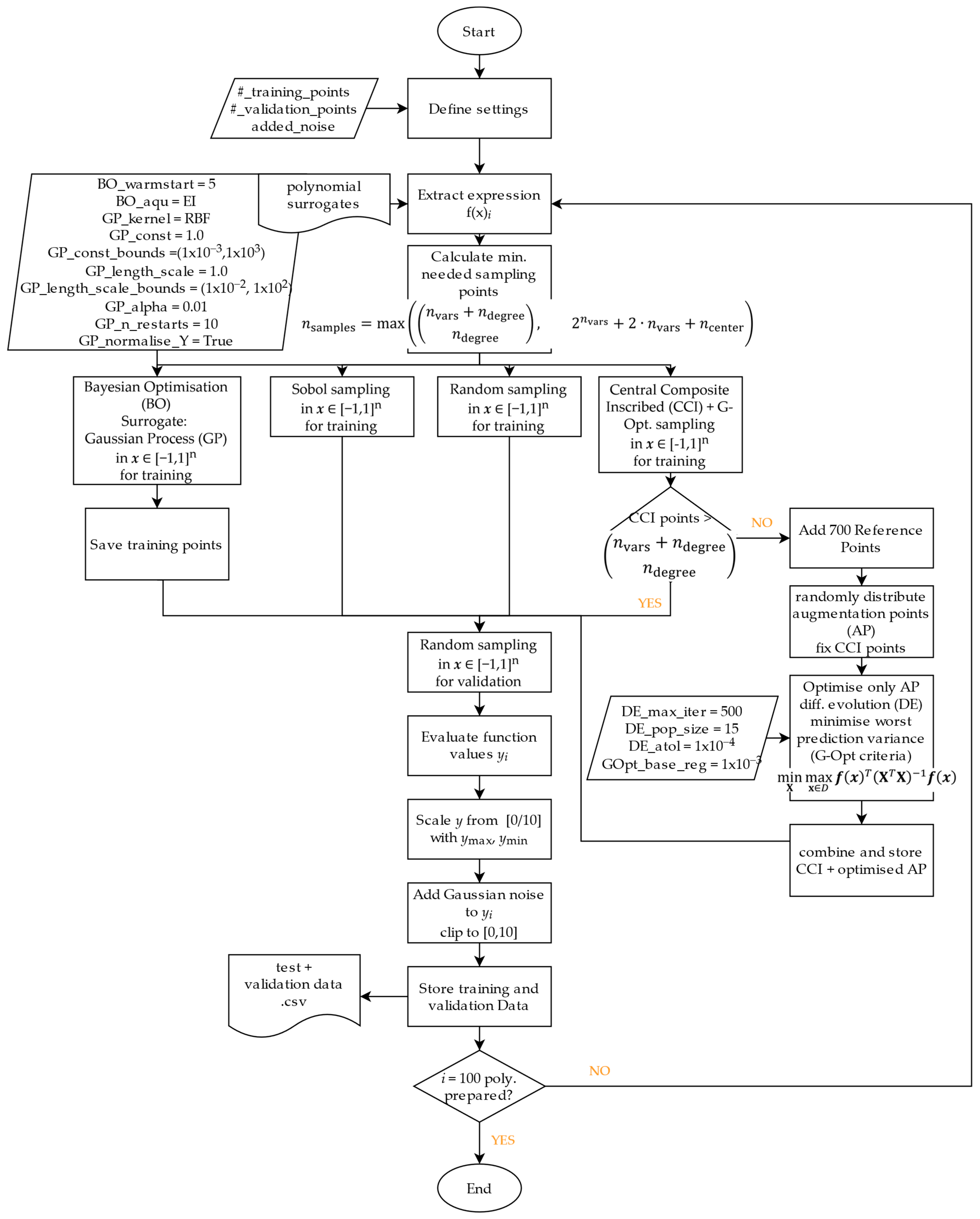
Figure A2.
Exemplary random forest surrogate modelling pipeline including hyperparameter optimisation, cross-validation, and model evaluation.
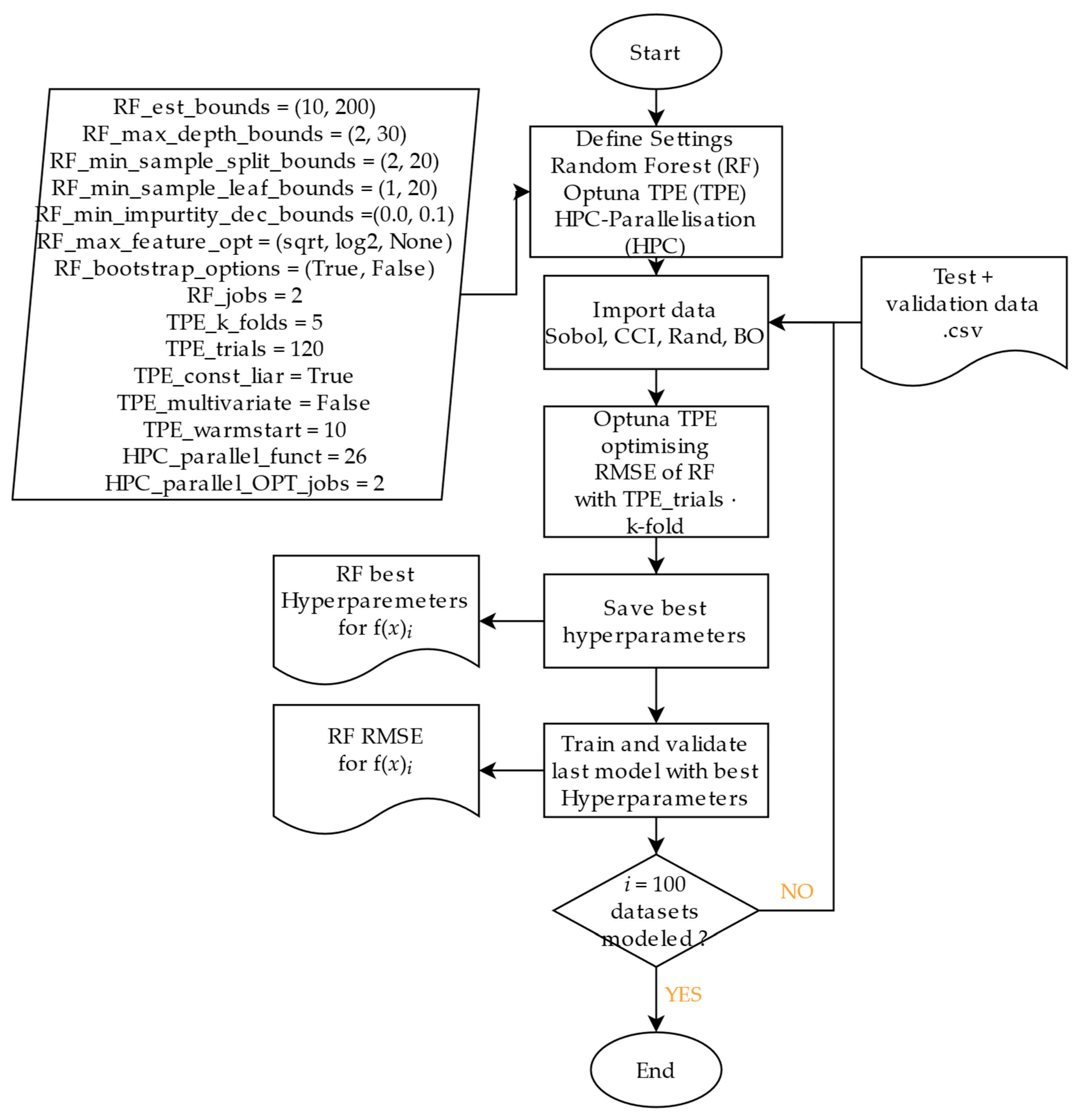
Table A1.
Hyperparameter settings to be optimised for each evaluated ML method.
Table A2.
Hyperparameter settings for optimiser evaluation with LightGBM as exemplary ML model.
Appendix B
Figure A3.
Workflow of the statistical evaluation pipeline, including outlier treatment, linear mixed-effects modelling, Wald tests, and effect size estimation.
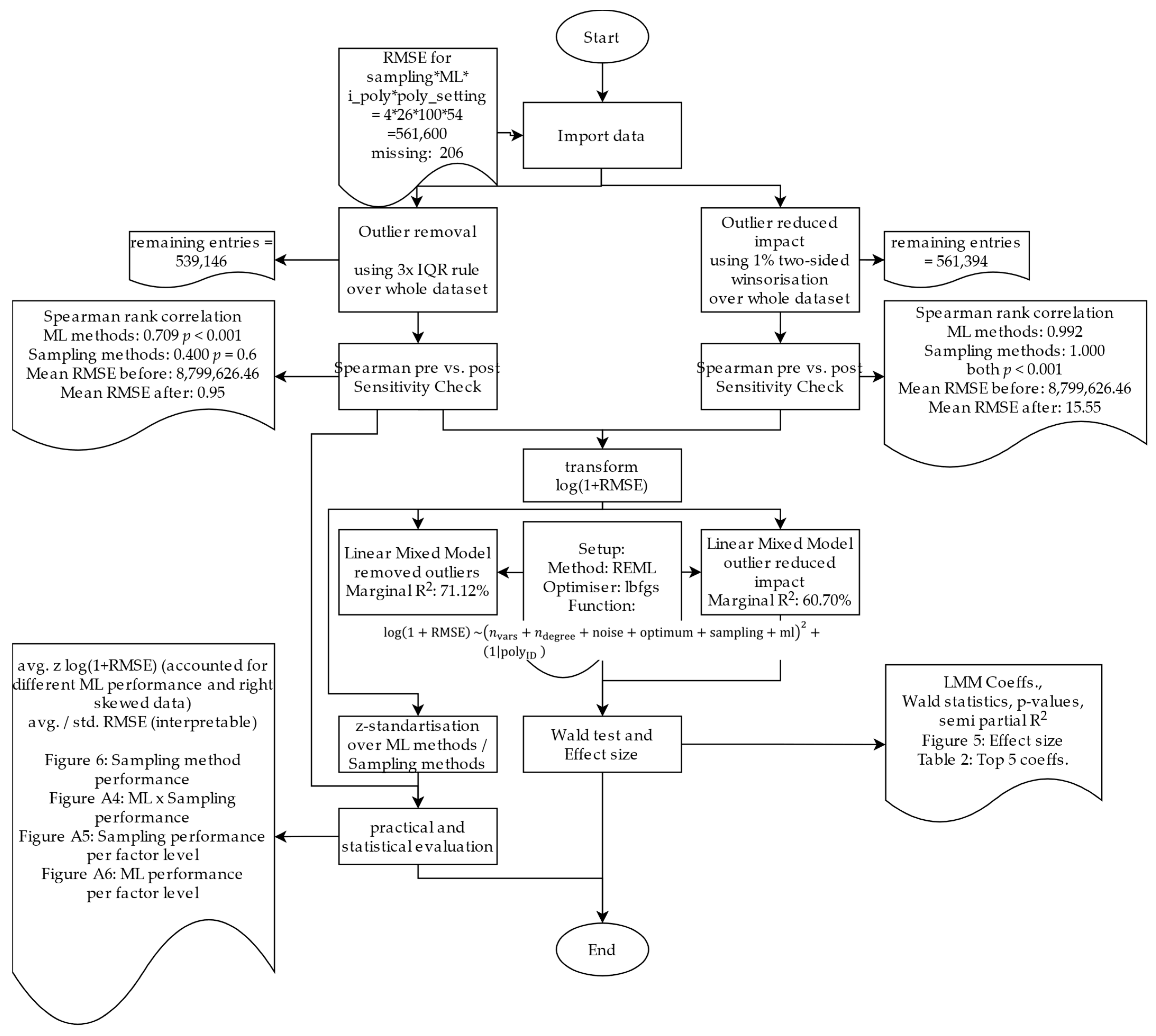
Figure A4.
Heatmap of the mean RMSE for each combination of ML and sampling method. Based on the dataset with removed outliers through 3x IQR Method.
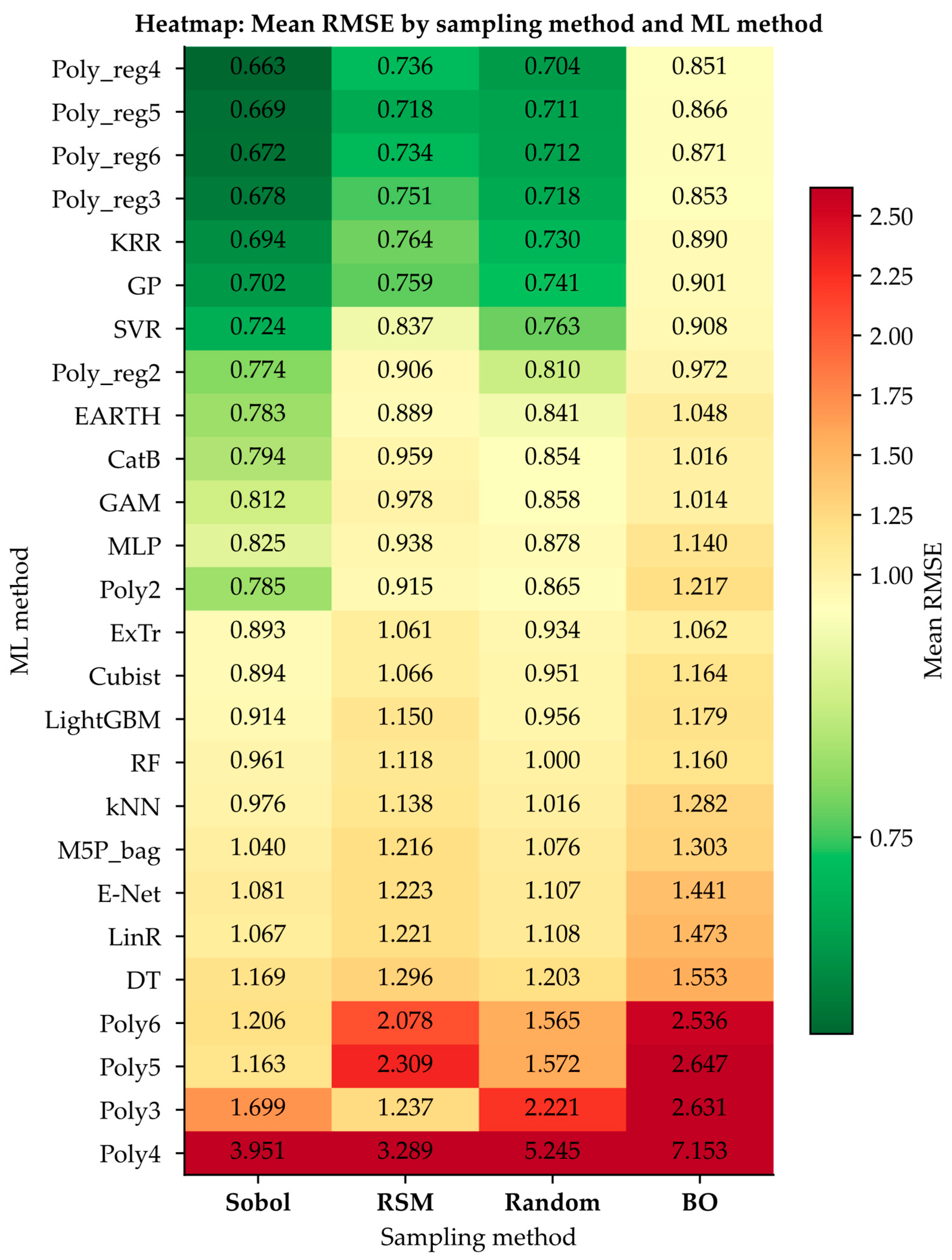
Figure A5.
Mean RMSE depending on (a) number of variables; (b) polynomial degree; (c) added Gaussian noise; (d) position of the optimum.
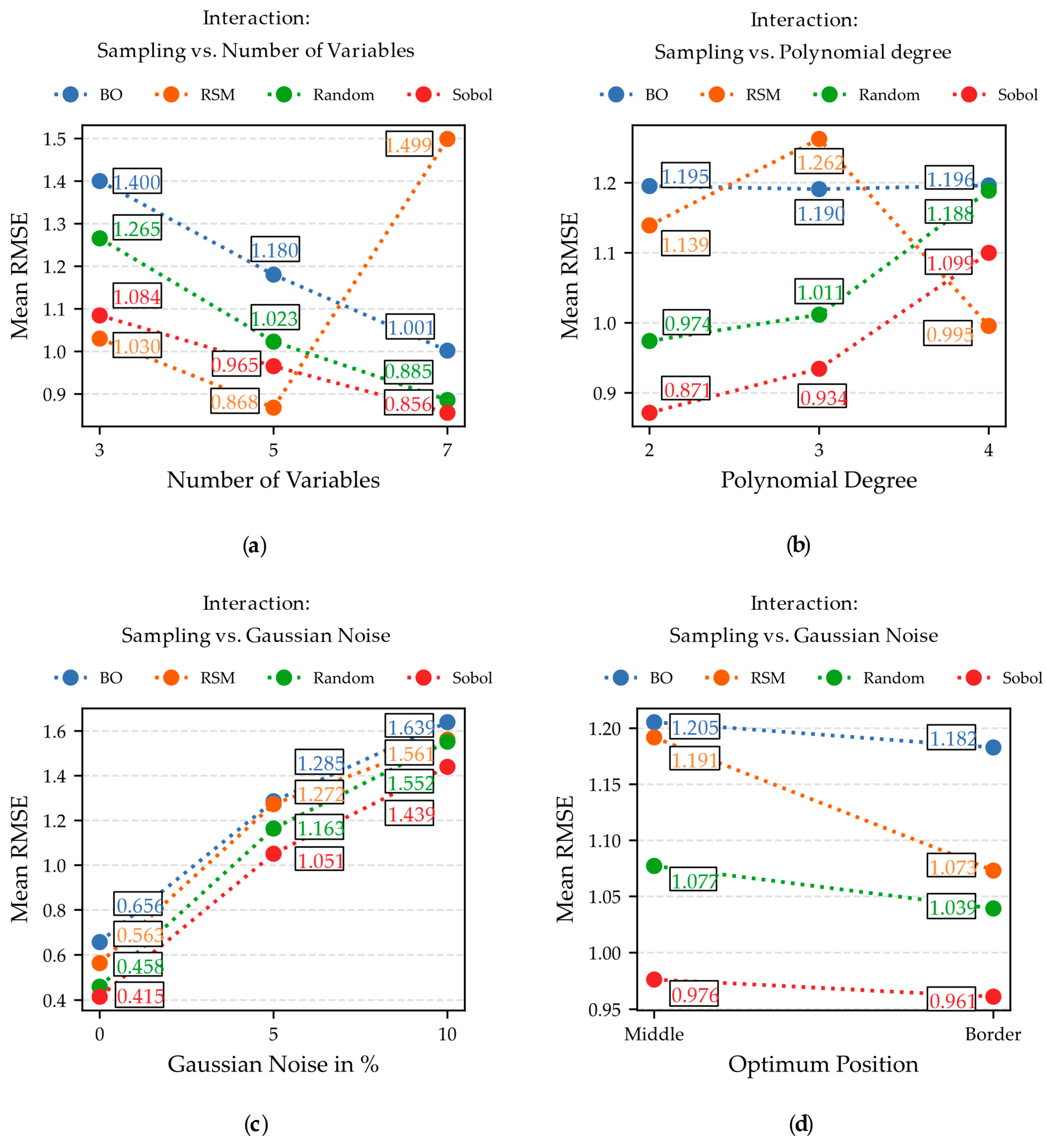
Figure A6.
ML ranking after mean RMSE depending on (a) number of variables; (b) polynomial degree; (c) added Gaussian noise; (d) position of the optimum.
Appendix C
Figure A7.
Meta decision tree with expected mean performance as a guideline for non-domain experts based on the study results. Colour gradient from green to red according to mean RMSE performance.
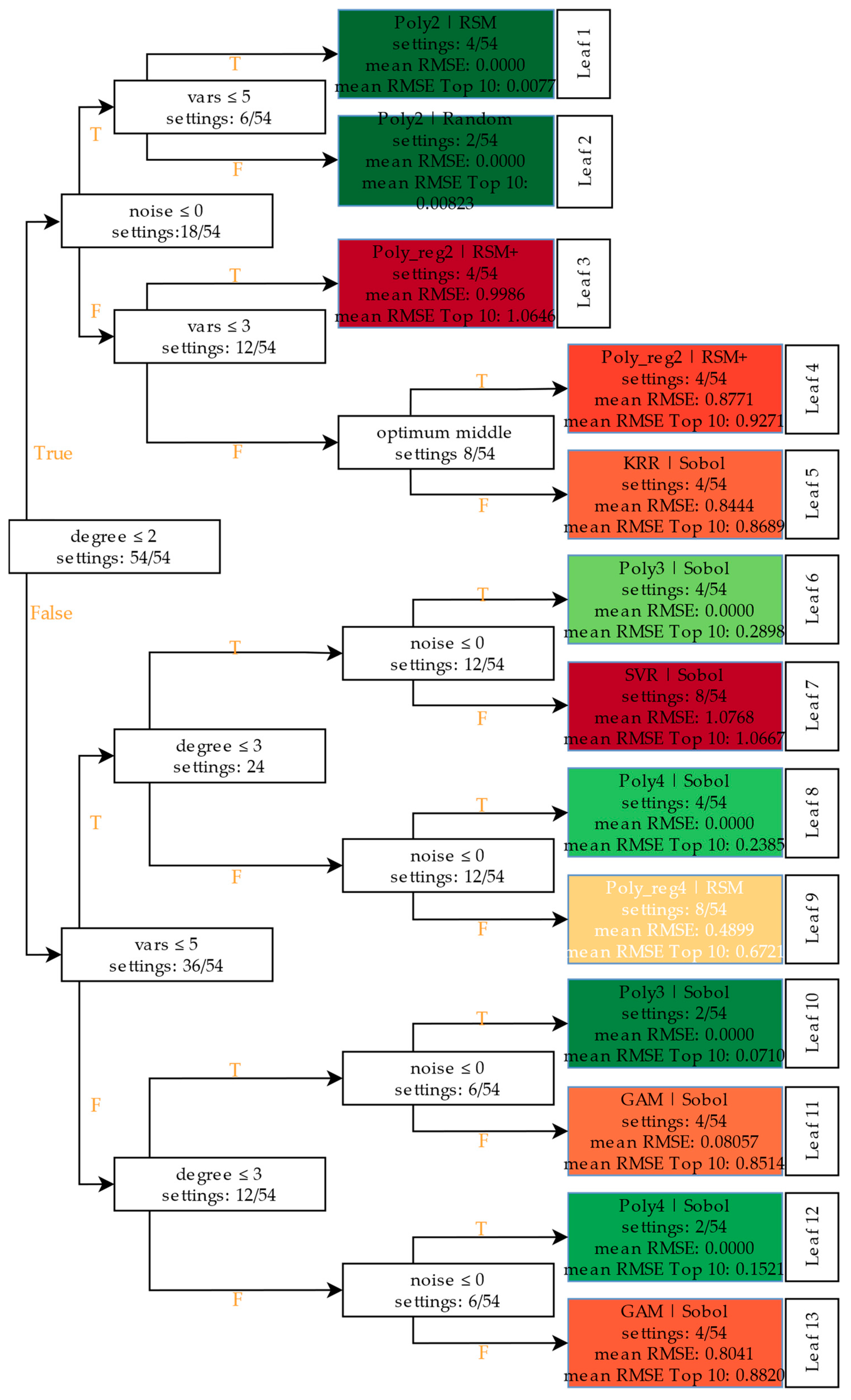
Figure A8.
Leaves 1–13 (a–m) from Decision Tree (Appendix C Figure A7)—Top 10 ML choices depending on the process/polynomial characteristics; without ML repetitions.
References
- Zéhil, G.-P.; Dib, N. A Brief Review of Simplified Modeling Approaches Commonly Used in Engineering. In Proceedings of the 2023 Fifth International Conference on Advances in Computational Tools for Engineering Applications (ACTEA), Zouk Mosbeh, Lebanon, 5–7 July 2023; IEEE: New York, NY, USA, 2023; pp. 109–114. [Google Scholar] [CrossRef] [Scilit]
- Arboretti, R.; Ceccato, R.; Pegoraro, L.; Salmaso, L. Design of Experiments and Machine Learning for Product Innovation: A Systematic Literature Review. Qual. Reliab. Eng. 2022, 38, 1131–1156. [Google Scholar] [CrossRef] [Scilit]
- Tercan, H.; Meisen, T. Machine Learning and Deep Learning Based Predictive Quality in Manufacturing: A Systematic Review. J. Intell. Manuf. 2022, 33, 1879–1905. [Google Scholar] [CrossRef] [Scilit]
- Kamiri, J.; Mariga, G. Research Methods in Machine Learning: A Content Analysis. IJCIT 2021, 10, 77–91. [Google Scholar] [CrossRef] [Scilit]
- El-Sanabary, S.; Kouta, H.; Shaban, M.; Alrumayh, A.; Alateyah, A.I.; Alsunaydih, F.N.; Alawad, M.O.; El-Taybany, Y.; El-Asfoury, M.S.; El-Garaihy, W.H. A Comparative Study of Machine Learning and Response Surface Methodologies for Optimizing Wear Parameters of ECAP-Processed ZX30 Alloy. Heliyon 2024, 10, e33967. [Google Scholar] [CrossRef] [Scilit] [PubMed]
- Murad, M.S.; Hamzat, A.K.; Unlu, N.A.; Altay, O.; Bahceci, E.; Asmatulu, E.; Bakir, M.; Asmatulu, R. Comparative Analysis of Machine Learning Models for Predicting the Mechanical Properties of Aerospace Grade Fiber Composites. Mach. Learn. Comput. Sci. Eng. 2026, 2, 20. [Google Scholar] [CrossRef] [Scilit]
- Lgayhardt Machine Learning Algorithm Cheat Sheet-Designer-Azure Machine Learning. Available online: https://learn.microsoft.com/en-us/azure/machine-learning/algorithm-cheat-sheet?view=azureml-api-1 (accessed on 16 August 2026).
- Hui, L. Which Machine Learning Algorithm Should I Use? Available online: https://blogs.sas.com/content/subconsciousmusings/2020/12/09/machine-learning-algorithm-use/ (accessed on 16 August 2026).
- Kumar, C.; Käppel, M.; Schützenmeier, N.; Eisenhuth, P.; Jablonski, S. A Comparative Study for the Selection of Machine Learning Algorithms Based on Descriptive Parameters. In Proceedings of the 8th International Conference on Data Science, Technology and Applications; SCITEPRESS-Science and Technology Publications: Prague, Czech Republic, 2019; pp. 408–415. [Google Scholar] [CrossRef] [Scilit]
- Sekeroglu, B.; Ever, Y.K.; Dimililer, K.; Al-Turjman, F. Comparative Evaluation and Comprehensive Analysis of Machine Learning Models for Regression Problems. Data Intell. 2022, 4, 620–652. [Google Scholar] [CrossRef] [Scilit]
- Gacto, M.J.; Soto-Hidalgo, J.M.; Alcalá-Fdez, J.; Alcalá, R. Experimental Study on 164 Algorithms Available in Software Tools for Solving Standard Non-Linear Regression Problems. IEEE Access 2019, 7, 108916–108939. [Google Scholar] [CrossRef] [Scilit]
- Pendurkar, S.; Huang, T.; Koenig, S.; Sharon, G. The (Un)Scalability of Heuristic Approximators for NP-Hard Search Problems. arXiv 2022, arXiv:2209.03393. [Google Scholar] [CrossRef] [Scilit]
- Cui, Z.; Gong, G. The Effect of Machine Learning Regression Algorithms and Sample Size on Individualized Behavioral Prediction with Functional Connectivity Features. NeuroImage 2018, 178, 622–637. [Google Scholar] [CrossRef] [Scilit] [PubMed]
- Roh, Y.; Heo, G.; Whang, S.E. A Survey on Data Collection for Machine Learning: A Big Data—AI Integration Perspective. arXiv 2019, arXiv:1811.03402. [Google Scholar] [CrossRef] [Scilit]
- Mohammed, S.; Budach, L.; Feuerpfeil, M.; Ihde, N.; Nathansen, A.; Noack, N.; Patzlaff, H.; Naumann, F.; Harmouch, H. The Effects of Data Quality on Machine Learning Performance on Tabular Data. Inf. Syst. 2025, 132, 102549. [Google Scholar] [CrossRef] [Scilit]
- Das, S.; Tesfamariam, S. State-of-the-Art Review of Design of Experiments for Physics-Informed Deep Learning. arXiv 2022, arXiv:2202.06416. [Google Scholar] [CrossRef] [Scilit]
- Joseph, V.R. Space-Filling Designs for Computer Experiments: A Review. Qual. Eng. 2016, 28, 28–35. [Google Scholar] [CrossRef] [Scilit]
- Siebertz, K.; Van Bebber, D.; Hochkirchen, T. Statistische Versuchsplanung; Springer: Berlin/Heidelberg, Germany, 2017; ISBN 978-3-662-55742-6. [Google Scholar] [CrossRef] [Scilit]
- Arboretti, R.; Ceccato, R.; Pegoraro, L.; Salmaso, L. Design Choice and Machine Learning Model Performances. Qual. Reliab. Eng. 2022, 38, 3357–3378. [Google Scholar] [CrossRef] [Scilit]
- Panico, A.; Corvi, A.; Collini, L.; Sciancalepore, C. Multi Objective Optimization of FDM 3D Printing Parameters Set via Design of Experiments and Machine Learning Algorithms. Sci. Rep. 2025, 15, 16753. [Google Scholar] [CrossRef] [Scilit] [PubMed]
- Lee, J.-N.; Lin, C.; Ferng, Y.-C.; Jen, K.-K.; Tsai, M.-H. Machine Learning-Based Process Optimization for Directed Energy Deposition of Aerospace Components. Appl. Sci. 2026, 16, 6170. [Google Scholar] [CrossRef] [Scilit]
- Weichert, D.; Houben, S.; Kister, A.; Ernis, G.; Wirtz, T. A Bayesian Approach to Adversarially Robust Life Testing. Available online: https://openreview.net/pdf?id=WgsuwfnXB2 (accessed on 16 August 2026).
- Rudin, W. Principles of Mathematical Analysis, 3rd ed.; International Series in Pure and Applied Mathematics; McGraw-Hill: New York, NY, USA, 2008; ISBN 978-0-07-054235-8. [Google Scholar]
- Joseph, V.R.; Gul, E.; Ba, S. Maximum Projection Designs for Computer Experiments. Biometrika 2015, 102, 371–380. [Google Scholar] [CrossRef] [Scilit]
- Renardy, M.; Joslyn, L.R.; Millar, J.A.; Kirschner, D.E. To Sobol or Not to Sobol? The Effects of Sampling Schemes in Systems Biology Applications. Math. Biosci. 2021, 337, 108593. [Google Scholar] [CrossRef] [Scilit] [PubMed]
- Chrisman, L. Pi Day Comparison: Monte Carlo vs Latin Hypercube vs Sobol Sampling. Available online: https://analytica.com/blog/pi-day-comparison-monte-carlo-vs-latin-hypercube-vs-sobol-sampling/ (accessed on 16 August 2026).
- Tarantola, S.; Becker, W.; Zeitz, D. A Comparison of Two Sampling Methods for Global Sensitivity Analysis. Comput. Phys. Commun. 2012, 183, 1061–1072. [Google Scholar] [CrossRef] [Scilit]
- Kucherenko, S.; Albrecht, D.; Saltelli, A. Exploring Multi-Dimensional Spaces: A Comparison of Latin Hypercube and Quasi Monte Carlo Sampling Techniques. arXiv 2015, arXiv:1505.02350. [Google Scholar] [CrossRef] [Scilit]
- Bogon, T. Agentenbasierte Schwarmintelligenz; Springer: Wiesbaden, Germany, 2013; ISBN 978-3-658-02291-4. [Google Scholar] [CrossRef] [Scilit]
- Willett, R.; Nowak, R.; Castro, R. Faster Rates in Regression via Active Learning. Available online: https://proceedings.neurips.cc/paper_files/paper/2005/file/4ea6a546c19499318091a9df40a13181-Paper.pdf (accessed on 16 August 2026).
- Qiu, S.; Qiu, K. Formulae for Slopes and Curvatures of Two Curves in Quadratic Polynomial Regression Equations with Response Surface Analysis. In Response Surface Methods—Theory, Applications and Optimization Techniques; Silva, V., Sousa Cardoso, J., Eds.; IntechOpen: London, UK, 2024; ISBN 978-0-85466-767-3. [Google Scholar] [CrossRef] [Scilit]
- Ozaki, Y.; Tanigaki, Y.; Watanabe, S.; Onishi, M. Multiobjective Tree-Structured Parzen Estimator for Computationally Expensive Optimization Problems. In Proceedings of the 2020 Genetic and Evolutionary Computation Conference, Cancún, Mexico, 8–12 July 2020; ACM: New York, NY, USA, 2020; pp. 533–541. [Google Scholar] [CrossRef] [Scilit]
- Mjgmario Hyperparameter Optimization with Optuna. Available online: https://medium.com/@mjgmario/hyperparameter-optimization-with-optuna-8fca06ea5491 (accessed on 27 September 2026).
- Hastie, T.; Tibshirani, R.; Friedman, J.H. The Elements of Statistical Learning: Data Mining, Inference, and Prediction, 2nd ed.; Springer Series in Statistics; Springer: New York, NY, USA, 2017; ISBN 978-0-387-84857-0. [Google Scholar]
- Wiesner, V.; Hornung, J.; Deinzer, F.; Rost, A.; Stark, M.; Trier, M. Sampling Techniques for Experimental Design in Additive Manufacturing: Testing the Accuracy of Machine Learning Models through Data Collection Methods to Improve the Mechanical Properties of Vat Polymerisation Resins. Prog. Addit. Manuf. 2026, 11, 6781–6791. [Google Scholar] [CrossRef] [Scilit]

Disclaimer/Publisher’s Note: The statements, opinions and data contained in all publications are solely those of the individual author(s) and contributor(s) and not of MDPI and/or the editor(s). MDPI and/or the editor(s) disclaim responsibility for any injury to people or property resulting from any ideas, methods, instructions or products referred to in the content. |
© 2026 by the authors. Licensee MDPI, Basel, Switzerland. This article is an open access article distributed under the terms and conditions of the Creative Commons Attribution (CC BY) license.