


Abstract
Reported gains from multimodal fusion, feature-attribution explanations, and model-confidence scores are only as trustworthy as the evaluation protocol and preprocessing pipeline behind them, yet these are rarely audited together. We develop a benchmarking-and-auditing methodology addressing four failure points jointly, subject-overlapping evaluation, class-imbalance correction under a subject-wise split, feature attribution, and calibration, instantiated on seven models under leave-one-subject-out (LOSO) cross-validation spanning three encoder-backbone pairings and early, late, and hybrid fusion, using VARISHTA-MM50, a synchronised IMU-and-video dataset of 50 elderly participants (aged 60–90). Random Forest under late fusion achieves the best LOSO accuracy (85.00%), outperforming every deep architecture tested. Subject-overlapping evaluation overstates accuracy by a mean of 8.32 percentage points; a GroupKFold control isolates subject overlap as the cause, and the effect replicates on an independent dataset. A leakage-safe oversampling protocol confirms the model ranking is not a preprocessing artefact. TreeSHAP attribution shows individual inertial features outweigh individual video features (1.32× per feature), though the wider video branch contributes more in aggregate, and a modality-removal ablation shows this dependence is specific to the tree ensemble. The most accurate model is the least well-calibrated by Expected Calibration Error. Subject-independent benchmarking, leakage auditing, attribution, and calibration form one connected evaluation discipline rather than four separate checks.
1. Introduction
Benchmark accuracy figures, post hoc feature-attribution explanations, and model-confidence scores are three of the most common outputs a machine learning pipeline is asked to produce, and each is routinely trusted on its own. In practice, each depends on preceding choices that are rarely audited together: an accuracy figure depends on whether the evaluation split is truly independent of the unit the model must generalise across; a class-imbalance correction step applied before that split can silently leak information across it; a feature-attribution explanation computed only in aggregate can obscure how unevenly a fused model actually draws on its inputs; and a confidence score is not guaranteed to track accuracy at all. This paper develops and demonstrates a benchmarking-and-auditing methodology that treats these four checks: a subject-independent evaluation protocol, leakage-safe preprocessing under that protocol, feature attribution, and calibration as one connected evaluation discipline rather than four separate, optional add-ons, and instantiates it on a multimodal (inertial-sensor + video) fusion case study.
Multimodal fusion, combining wearable inertial sensors with video, is routinely assumed to improve human activity recognition (HAR) over single-modality baselines. Yet, this assumption is rarely tested under conditions that matter for deployment: subject-independent evaluation, where a model must generalise to a person it has never seen during training. Most published HAR results use subject-overlapping random splits, which can substantially overstate real-world generalisation [1,2]. Whether fusion still helps once this optimistic evaluation protocol is replaced with leave-one-subject-out (LOSO) cross-validation, and which fusion strategy benefits which model class, have not been systematically characterised.
This question is especially consequential for elderly-focused HAR and fall detection, where inertial sensors alone cannot reliably separate activities with similar acceleration signatures (e.g., descending stairs versus a walk-and-fall), and video alone does not capture the millisecond-scale impact transient that distinguishes a genuine fall from a controlled sit-down. Fusing both modalities is a natural response, but three gaps limit systematic study of this problem. Gap 1: Existing multimodal HAR resources with fall-inclusive labels are largely built on Western, younger cohorts [3,4,5,6], leaving open how fusion behaves on populations with distinct gait kinematics, footwear conventions, and garment-sensor coupling effects. Gap 2: No benchmark evaluates a broad span of fusion mechanisms, feature concatenation, late probability fusion, and each architecture’s native cross-modal mechanism against one another on the same synchronised sensor-video data. Gap 3: Almost no prior multimodal HAR study reports LOSO evaluation, so it is unclear whether fusion gains reported under random splits survive subject-independent testing.
Beyond these three, a fourth gap is equally consequential but far less often addressed explicitly: Gap 4, whether a benchmark’s own auxiliary engineering choices, most concretely, how class-imbalance correction is implemented under LOSO, are themselves LOSO-safe. Class-imbalance techniques such as SMOTE and its variants are routine in the HAR literature, but are typically validated for accuracy alone, not for subject-independence: naive application before a subject-wise split is a known, general failure mode wherever class-imbalance correction interacts with subject-independent evaluation, since it can leak a held-out subject’s identity into training through synthetic-sample interpolation, silently inflating exactly the kind of subject-independent accuracy figure a benchmark otherwise takes care to report honestly. Our oversampling protocol is designed to guard against this failure mode by construction, with the design verified empirically. This is one instance of a broader point this paper argues throughout: a subject-independent accuracy figure is not, by itself, sufficient grounds for a deployment decision, since it can rest on an unverified preprocessing step, obscure how unevenly a model draws on its available modalities, or overstate how much its confidence scores can be trusted. Verifying every subject-aware step in the pipeline, not only the train/test split, is a necessary first check; the same standard of scrutiny extends naturally to asking why a model reaches its predictions and whether its confidence can be trusted.
This paper addresses all four gaps with a single benchmarking-and-auditing methodology, instantiated on one case study rather than four disconnected demonstrations. We introduce VARISHTA-MM50, a synchronised dual-modality (IMU + video) dataset of 50 elderly participants across nine activity classes, and use it to benchmark seven models: SVM, Random Forest, CNN + LSTM, BiLSTM, UMMAE, Cross-AE, and Perceiver IO, under sensor-only, video-only, and fused configurations, across three encoder-backbone pairings and early, late, and hybrid fusion, with LOSO as the primary evaluation protocol throughout. The elderly-care fall-detection setting is a natural and consequential choice for this case study precisely because it makes every one of the four failure points concrete and high-stakes, but the evaluation methodology itself, subject-wise protocol auditing, leakage-safe imbalance correction, joint unimodal-versus-fused attribution, and calibration-versus-accuracy analysis, generalises directly to any multimodal learning pipeline evaluated under a subject- or group-wise split.
Contributions
The contributions of this work are as follows:
- A benchmarking-and-auditing methodology that connects four evaluation checks that are normally reported separately, or not at all, subject-independent protocol design, leakage-safe preprocessing under that protocol, joint unimodal-versus-fused feature attribution, and calibration analysis, into a single reusable procedure applicable to any multimodal learning pipeline evaluated under a subject- or group-wise split, demonstrated here on multimodal fusion for human activity recognition (HAR) with 42 model×fusion configurations (seven models, three encoder-backbone pairings, three fusion strategies).
- An empirical finding that multimodal fusion consistently outperforms unimodal baselines under LOSO for all seven models, but that the late-versus-early fusion benefit is model-dependent rather than uniform.
- A targeted 80/20 random-split ablation directly addressing Gap 3: subject-overlapping evaluation overstates accuracy by a mean of 8.32 percentage points under late/hybrid fusion (range: to pp across all seven models) relative to LOSO, an effect that is negligible under early fusion and consistently smaller for cross-modal autoencoder/attention architectures than for classical and temporal models. The same contrast is then tested under a matched GroupKFold control, which holds training- and test-set size constant so that subject overlap is the only variable, and replicated on an independent dataset (Section 5.4).
- A model-selection protocol that extends the same leakage discipline to hyperparameter choice: all searched values are fixed on a disjoint group of subjects and frozen before the reported sweep, so that no test subject informs any configuration decision (Section 4.4). Reported as a control rather than a claim, it shows the model ranking is unchanged by the constraint.
- A leakage-safe oversampling protocol for subject-independent evaluation (Section 6), addressing Gap 4, with empirical verification (fold-count, group-label, and class-balance checks, plus a PCA projection of real versus synthetic samples) that the protocol carries no subject-identity leakage, and is applied throughout this benchmark; this verification procedure is itself directly reusable for any per-fold class-imbalance correction under a subject-wise split, independent of the HAR domain.
- A demonstration that the accuracy figures, by themselves, are an incomplete basis for a deployment decision: TreeSHAP-based feature attribution for the best-performing configuration, extended by a modality-removal ablation across the four late-fusion architectures that establishes how far a single model’s attribution pattern generalises (Section 7.4), and a calibration analysis testing whether the random-split evaluation gap already shown for accuracy extends to model confidence, reported with subject-level bootstrap intervals and proper scoring rules so that the comparison between architectures is quantified rather than asserted.
- A public benchmark dataset, VARISHTA-MM50, and companion evaluation code, released to support reproducible multimodal benchmarking and auditing research.
Table 1 summarises the four-part benchmarking-and-auditing methodology in generic form, alongside its concrete instantiation in this paper, so that the methodology can be read and reused independently of the HAR case study that follows.
Table 1.
The four-part benchmarking-and-auditing methodology in generic form (left) and as instantiated in this paper’s multimodal HAR case study (right). Each check is a precondition for trusting the one commonly reported in its place (accuracy, an attribution map, or a confidence score).
The remainder of this paper is organised as follows. Section 2 reviews HAR fusion methods and existing work on responsible and explainable AI for HAR and fall detection. Section 3 describes the VARISHTA-MM50 dataset. Section 4 details feature extraction, fusion strategies, and model architectures. Section 5 reports the benchmark results, including a comparison against prior published HAR systems. Section 6 presents the leakage-safe oversampling protocol and its empirical verification. Section 7 reports TreeSHAP-based explainability results. Section 8 reports the calibration analysis. Section 9 discusses the findings, and Section 10 and Section 11 cover limitations and conclusions, respectively.
2. Related Work
2.1. HAR Models and Multimodal Fusion
Sensor-based HAR has progressed from classical SVM and Random Forest on handcrafted inertial features [7] to CNN, LSTM, and hybrid CNN + LSTM temporal architectures that learn motion patterns directly from raw sequences [8,9]. Reported comparisons find LSTM outperforming classical ML on both a general-population and a small elderly-specific cohort, but at higher computational cost, while classical SVM remained the fastest option [7], a trade-off consistent with this paper’s own finding that a well-fused classical model can match or beat deep architectures. Attention-augmented hybrid CNN-BiLSTM models have also been applied specifically to elderly fall detection, reporting accuracy above 99% on KFall and MobiAct under random-split evaluation [10], and a parallel CNN-Transformer architecture combining local convolutional features with long-range Transformer attention has reported similarly high accuracy on SisFall and MobiAct [11], reinforcing the relevance of transformer-based cross-attention mechanisms such as Perceiver IO for this domain.
Transformer-based models, including Perceiver IO [12], handle heterogeneous multimodal inputs via cross-attention and show promise for synchronised sensor-video streams [9,13]. Unsupervised cross-modal autoencoders learn aligned latent representations without paired labels, which is attractive when labelled multimodal data is scarce [9]. Video-based HAR with VideoMAE [14] and spatiotemporal CNNs provides complementary postural cues to inertial signals [15,16,17,18], but vision-based systems are almost exclusively evaluated on single-modality benchmarks in controlled environments, and fusion-strategy choice (concatenation versus late probability fusion versus a model’s native cross-modal mechanism) is rarely compared directly within a single study. The same complementarity principle operates within the visual domain: Chen et al. [19] classify fine-grained assembly activities by combining RGB and hand-skeleton streams in a two-stage network that first extracts scene-level features from each visual modality and then models their temporal evolution with a recurrent classifier, reporting over 99% accuracy on trimmed clips and over 91% on untrimmed continuous activity. That result reinforces the premise underlying the fusion comparison in this paper, namely that distinct information sources contribute unequally to a recognition decision and that where in the pipeline they are combined materially affects the outcome. It also illustrates the evaluation gap this paper targets: as with most fine-grained activity work, those figures are obtained without subject-independent validation, so the extent to which they reflect generalisation to an unseen worker rather than to unseen clips of seen workers is not established. Prior multimodal fusion work for fall detection has largely combined depth or vision with motion cues rather than synchronised IMU and RGB video: a dual-stream framework fusing monocular depth and motion-history images achieved a 98.87% F1-score on UP-Fall but degraded under occlusion and low light [20], a cross-attention fusion of video and audio streams (Fall-Mamba) reported 98.94% accuracy while remaining sensitive to blocking interference and edge-deployment cost [21], and a federated residual-fusion framework combining wearable and camera streams on UP-Fall reported 95.27% accuracy while highlighting the difficulty of handling imbalanced or missing modalities [22].
2.2. Existing HAR Datasets and the Evaluation Gap
Standard benchmarks such as UCI-HAR, WISDM, MobiAct and HARTH target younger adult cohorts and are single-modality (IMU only) [3,23,24]; mHealth similarly targets younger, non-elderly participants performing general activities rather than falls [25]. SisFall, FALLAllD, and UMAFall include fall events but likewise lack a video modality [4,26,27]. Large-scale real-world fall repositories such as FARSEEING collect genuine falls from both young and elderly cohorts, but provide no structured ADL taxonomy and no video [28]; SmartFall aggregates multiple wrist- and torso-worn sources but is severely class-imbalanced between falls and ADLs [29].
Video-inclusive datasets are markedly rarer in this literature, for reasons that reinforce this paper’s motivation: camera-based collection raises privacy concerns that wearables do not, is more costly and logistically harder to scale, and is almost never conducted with elderly participants specifically. Among datasets that do combine video with inertial data, URFD pairs two Kinect cameras (RGB and depth) with a wireless accelerometer, but from only 5 (non-elderly) subjects across 70 sequences [30]; its subject count is smaller than the number of folds a meaningful LOSO evaluation would require, and no LOSO result is reported for it in the literature. The closest multimodal resource at larger scale, UP-Fall, provides IMU, EEG, and RGB data but targets young adults aged 18–24 [31]; HAR70+ targets an elderly cohort but is accelerometer-only, without falls or video [6]. Across every video-inclusive dataset surveyed here, video-only or multimodal, none reports subject-independent (LOSO) evaluation, and none reaches a subject count comparable to this paper’s 50 participants, which is precisely the combination:video modality, elderly cohort, and a subject count sufficient for leave-one-subject-out evaluation, that VARISHTA-MM50 is designed to provide. Table 2 summarises this comparison of VARISHTA-MM50 against the datasets discussed above.
Table 2.
Comparison of relevant public HAR datasets against VARISHTA-MM50, grouped by modality.
2.3. Responsible and Explainable AI for HAR and Fall Detection
A separate line of work asks not whether a HAR or fall-detection model is accurate, but whether its predictions can be trusted and understood, which is the specific gap Section 6, Section 7 and Section 8 of this paper address. Salih et al. provide a general perspective on the two dominant post hoc explanation frameworks, SHAP and LIME [34], both of which have been applied specifically to HAR: Tempel et al. use SHAP to explain a graph convolutional HAR model on skeleton data, introducing a perturbation-based protocol to validate that the resulting explanations are not just plausible-looking but quantitatively faithful to the model [35], and in a companion study directly compare SHAP against Grad-CAM for HAR, finding the two methods highlight different, only partially overlapping evidence for the same prediction [36]. Kaushik et al. similarly combine several classical HAR models with post hoc explainability methods to identify which handcrafted features drive classification [37]. Closest to this paper’s own combination of concerns, Bragança et al. use SHAP explanations specifically to diagnose why different validation strategies, including LOSO, produce different accuracy estimates for the same HAR model, showing that explanation and evaluation-protocol honesty are linked rather than separate concerns [38].
Explainability for fall detection specifically has been addressed largely within a single modality at a time, which the fused explainability analysis of Section 7 directly extends beyond. Mankodiya et al. apply LIME to a sequence model trained on multiple wearable inertial sensors, using the resulting explanations to identify which sensor placement contributes most to a fall prediction [39]; their attribution is confined to inertial features only, with no video modality present to attribute against or trade off. Dutt et al. take the complementary video-only approach, proposing a modular deep learning architecture for video-based fall detection designed for interpretability by construction rather than only via post hoc attribution [40]; conversely, their interpretability is confined to visual evidence, with no inertial signal in the model at all. Chakraborty et al. apply explainable AI to gait-based fall detection and explicitly compare smartphone- and wearable-sensor-derived explanations [41], the closest prior work to this paper’s own modality-attribution question, but their comparison remains within a single modality (two inertial-sensor placements), not across modalities. To our knowledge, no prior explainability study in this space applies SHAP-based attribution jointly across inertial and video modalities within a single fused fall-detection model.
On calibration, Roy et al. propose a confidence-calibrated HAR ensemble that averages predictions across multiple temporal window sizes, showing this improves calibration without sacrificing accuracy [42], a direct precedent for this paper’s finding that calibration and accuracy are governed by different properties of a model rather than moving together automatically. That precedent evaluates calibration only for single models in isolation; Section 8 of this paper extends the comparison across seven architecturally distinct models and across two evaluation protocols (LOSO and 80/20), showing that the protocol choice itself, not only model choice, materially affects reported calibration.
2.4. Evaluation Integrity and Leakage as a General Machine Learning Problem
The evaluation-protocol and leakage concerns this paper raises for HAR specifically are instances of failure modes documented across machine learning-based science broadly, not artefacts unique to this domain. Kapoor and Narayanan survey machine learning-based research across seventeen scientific fields and identify a taxonomy of eight distinct leakage types, affecting at least 294 published papers, several of which involve exactly the preprocessing-before-split pattern this paper’s leakage-safe oversampling protocol is designed to rule out [43]. Their central argument, that a reported accuracy figure is only as trustworthy as the independence of the evaluation split and every preprocessing step conducted before it, is the general form of this paper’s Gap 4 and Section 6. Separately, Recht et al. show that image classifiers trained and tuned against a fixed, heavily reused test set suffer substantial accuracy drops on a newly collected but distributionally matched test set [44], a general-vision precedent for this paper’s own finding that subject-overlapping evaluation systematically overstates accuracy relative to a genuinely held-out protocol (Section 5.3), even though the underlying mechanism differs: implicit test-set reuse in their case, explicit subject overlap in ours. Closer to this paper’s specific combination of accuracy, attribution, and calibration concerns, Liu and Zhu propose an ensemble-disagreement-based uncertainty measure for imbalanced fraud detection, showing that a model’s own confidence, not only its accuracy, determines whether it can be safely deployed with human review reserved for the cases it is genuinely unsure about [45]; their finding that accuracy and usable confidence are separate properties of a model, addressed in a non-medical, non-HAR imbalanced-classification setting, is a direct cross-domain precedent for this paper’s own calibration-versus-accuracy divergence (Section 8).
3. VARISHTA-MM50 Dataset and Acquisition Protocol
VARISHTA-MM50 provides the synchronised multimodal, fall-inclusive, subject-diverse substrate needed to evaluate fusion strategies under LOSO. Fifty Indian elderly participants, recruited in and around Maharashtra, were sampled across five collection batches, spanning a senior citizen care home, private residences, and community parks, with fall trials supervised by a trained caregiver throughout. As Table 2 shows, existing elderly-focused HAR datasets (e.g., HAR70+, WEDAFALL) draw on Western populations and are IMU-only, while existing video-inclusive multimodal datasets (URFD, UP-Fall) draw on non-elderly cohorts; to the best of our knowledge, no prior public HAR resource combines an elderly cohort from the Indian subcontinent, synchronised IMU-and-video fusion, and a subject pool large enough to support leave-one-subject-out evaluation, a combination this dataset is specifically designed to provide. Two smartphones were used per session: one running Sensor Logger [46] to record tri-axial accelerometer, gyroscope, and orientation streams at 50 Hz, and a second recording synchronised 1080 p video at 30 fps. The sensor device was carried in naturalistic positions (hand-held, pocket, or waist pouch), introducing realistic placement variability rather than a single fixed mount point.
Nine activity classes were recorded: six activities of daily living (ADLs) and three fall types. ADL trials lasted approximately 30 s; fall trials 20–25 s, reflecting both the inherently brief nature of a fall event and a personal-safety consideration for this cohort: each fall trial was stopped as soon as the caregiver confirmed the fall-and-recovery sequence was complete. Each trial yields three synchronised CSV files (accelerometer, gyroscope, orientation) and one MP4 file, linked by a shared trial identifier, and the dataset is organised hierarchically by activity class and participant. Full acquisition and annotation detail, ethics approval information, and directory-structure documentation are provided with the released dataset. Figure 1 summarises this modality-and-activity structure schematically.
Figure 1.
VARISHTA-MM50 modality and activity taxonomy at a glance.
4. Feature Extraction, Models, and Evaluation Protocol
Figure 2 summarises the full benchmark pipeline described in this section: unified feature extraction, three fusion strategies and the LOSO evaluation protocol, and the seven model architectures compared.
Figure 2.
End-to-end benchmark pipeline for multimodal HAR: sensor and video encoding, fusion, and classification under LOSO cross-validation.
4.1. Inertial and Video Feature Extraction
A unified feature pipeline is applied across all seven architectures to isolate model- and modality-specific effects from preprocessing effects. Inertial signals are resampled to 30 Hz to match the video frame rate, z-score normalised per recording using that recording’s own statistics only, and low-pass filtered (Butterworth, 20 Hz). Sliding windows of 3 s (90 samples, 50% overlap) are extracted from the nine tri-axial channels; a 3 s window (longer than the 1–2 s windows typical in younger-cohort HAR) is used to capture the slower gait, slower sit-down, and full pre-fall-to-impact sequence characteristic of elderly movement. Each window is passed through TinyHAR [47], a lightweight architecture combining depthwise Conv1D, cross-channel attention, pointwise channel expansion, temporal convolution, and temporal-attention pooling targeted at fall-impact peaks, producing a 128-D inertial feature vector.
On the video side, features are extracted with X3D [48], a lightweight 3D convolutional network pretrained on Kinetics-400. Because Kinetics-400 is dominated by younger, sports-oriented activity classes, the first three X3D stages are frozen and the last two fine-tuned on VARISHTA-MM50 (20 epochs, AdamW, cosine annealing, class-weighted cross-entropy with fall-class upweighting), producing a 256-D video feature vector. X3D is selected for its favourable accuracy-to-compute trade-off (3.76 M params, 4.73 GFLOPs), consistent with the low-cost acquisition philosophy of Section 3. To test whether results generalise beyond one encoder pairing, a general-purpose 1D-CNN [49,50] and VideoMAE [14] (a masked-video pretraining transformer, 87 M parameters) are substituted for TinyHAR and X3D respectively, giving three encoder-backbone pairings evaluated throughout: TinyHAR+X3D, 1D-CNN+VideoMAE, and X3D+1D-CNN (Table 3).
Table 3.
Encoder backbones evaluated across the three pairings.
4.2. Fusion Strategies and Evaluation Protocol
Three fusion strategies are compared rather than a single fixed scheme, differing in where in the pipeline sensor and video information are allowed to interact.
Early fusion concatenates independently normalised sensor and video feature vectors into a single 384-D representation before any classification decision is made, as shown in Figure 3; the sensor encoder’s 128-D output and the video encoder’s 256-D output are simply stacked into one vector, which a single downstream classifier (SVM, Random Forest, an LSTM head, depending on the model) then maps to a nine-way softmax. The two modalities are never separated again after this point, so any classifier weight that reacts to sensor evidence can also condition on video evidence in the same decision boundary. Late fusion instead trains two fully independent, single-modality classifiers end-to-end, each with its own encoder and its own classifier head, and combines only their output class-probability vectors at inference time via a fixed convex combination with (Figure 4). Neither branch ever observes the other modality during training, so late fusion cannot learn any cross-modal interaction, only a fixed-weight vote between two independently confident opinions; it is evaluated for the four classical/temporal models (SVM, RF, CNN + LSTM, BiLSTM), which have no built-in cross-modal mechanism to exploit instead.
Figure 3.
Early fusion. Independently normalised sensor and video embeddings are concatenated into a single 384-D vector before any classification decision is made, so a single joint classifier learns one decision boundary across both modalities together.
Figure 4.
Late fusion. Two fully independent, single-modality classifiers are trained end-to-end and combine only their output class-probability vectors.
Hybrid fusion, shown in Figure 5, refers to each deep architecture’s own, purpose-built cross-modal mechanism, evaluated in place of simple concatenation for the three models that have one (UMMAE, Cross-AE, Perceiver IO), since averaging their predictions (as late fusion does) would not exploit the mechanism each is specifically designed around. Unlike early and late fusion, hybrid fusion has no single fixed operation: sensor and video information interact inside the network, through whichever cross-modal interaction layer each architecture defines for itself. UMMAE and Cross-AE encode each modality to its own latent via a modality-specific encoder and use a reconstruction objective, self-reconstruction for UMMAE, and additionally cross-modal reconstruction for Cross-AE (each modality’s latent is decoded into a prediction of the other modality, which directly penalises an encoder that discards information the other modality would need), to keep each latent modality-informative before the two are concatenated and passed to a fusion MLP and classifier. Perceiver IO instead projects both modalities into a shared token space and lets a small learned latent array attend into it via cross-attention, with no reconstruction loss at all; cross-modal mixing is driven entirely by the attention weights the network learns.
Figure 5.
Hybrid fusion, general concept. Rather than mixing modalities only at the input (early fusion) or only at the output (late fusion), hybrid fusion lets sensor and video information interact inside the network, through a cross-modal interaction layer whose exact mechanism differs by architecture.
Evaluation uses leave-one-subject-out (LOSO) cross-validation across all 50 participants: each fold trains on 49 subjects and tests on the held-out participant, matching the deployment scenario of generalising to an unseen individual. SMOTE oversampling is applied within each training fold to balance the nine activity classes, and fall-class posterior probabilities are upweighted by a factor of 1.5. Both the upweighting factor and the fusion weight w were selected as operating points rather than tuned for accuracy, and Table 4 reports the sensitivity of the results to each. The boost costs Random Forest 0.56 pp of accuracy () and returns 5.61 pp of fall recall (); larger factors buy further recall but collapse fall precision from 90.0% to 68.9%. The lower panel repeats the comparison at this operating point for every architecture: the exchange rate is strongly model-dependent and most favourable for Random Forest, the configuration Section 9 recommends, while for the three cross-modal architectures the boost is close to inert and none of their changes is significant. For w, a sweep in steps of 0.05 finds optimal for SVM and Random Forest, while CNN + LSTM and BiLSTM peak slightly toward video ( and ); subject-wise nested selection of w changes accuracy by to pp and is not significant for any model, so the fusion-strategy conclusions do not depend on this choice. Adaptive per-sample weighting is untested and is left to future work.
Table 4.
Sensitivity to the two fixed operating points. Top left: fall-class boost swept for Random Forest. Top right: fusion weight, LOSO accuracy. Bottom: effect of the boost actually used, from 1.0 to 1.5, on every architecture in the benchmark. The three cross-modal models have no fusion weight, so the top-right panel does not apply to them.
Deep models are trained with AdamW (, weight decay ), cosine annealing (40 epochs), and label smoothing (); classical models use balanced class weights with standard feature scaling.
4.3. Model Architectures
Seven models spanning four paradigms are benchmarked. Classical baselines: SVM (RBF kernel, , balanced class weights) and Random Forest (100 trees, balanced class weights), both operating on the full feature vector (128-D, 256-D, or 384-D depending on configuration). Temporal deep learning: CNN + LSTM (1D-CNN feature extractor plus a 2-layer LSTM, 128 hidden units) and BiLSTM (bidirectional, 128 units per direction), exploiting pre- and post-event temporal context. Unsupervised cross-modal autoencoders: UMMAE trains modality-specific encoder–decoder pairs with a joint reconstruction and classification loss; Cross-AE additionally reconstructs each modality from the other, forcing encoders to capture cross-modally relevant features. Transformer-based fusion: Perceiver IO [12] projects both modalities into a shared byte array and applies cross-attention against a compact latent array for classification.
4.4. Model Selection Protocol
To establish that the reported ranking does not depend on hyperparameters chosen with test-subject information, ten participants (Person 16, 20, 22, 28, 29, 33, 35, 42, 48, 51) were separated before any model was fitted. The ten were drawn uniformly at random without replacement from the fifty subject identifiers under a fixed seed, so the split is reproducible from the released code and no measured result influenced it. Twenty per cent was taken as the smallest holdout that still exposes every activity class to the search: the drawn group covers all nine classes, and its per-subject difficulty is statistically indistinguishable from that of the remaining forty (mean fused LOSO accuracy 86.97% versus 85.23%, Welch p = 0.77, Mann–Whitney p = 0.79), so the frozen hyperparameters were not selected on an unrepresentatively easy or hard subset. All searched hyperparameters were selected on that group alone, frozen, and the LOSO sweep was re-run over the remaining forty subjects with the selection group excluded entirely (Table 5). The search selects for the SVM, whereas the main sweep of Section 4 uses ; for Random Forest, it confirms the 100 trees already used. Table 5 therefore reports what the benchmark becomes when the selection-group value is imposed in place of the published one, which is the quantity a leakage control has to measure. The fusion weight is treated separately in Section 4.2. Nested cross-validation within each of the fifty outer folds was computationally prohibitive across seven architectures and three encoder pairings, and a disjoint selection group provides the same guarantee at a fraction of the cost.
Table 5.
Leakage control. The original configuration is recomputed on the same forty subjects so that the effect of freezing hyperparameters is separated from the effect of the smaller subject set. Only SVM and Random Forest had hyperparameters in the search; the two deep rows repeat the same protocol with nothing selected, and so measure retraining variance alone, giving a noise floor for the two rows above.
Roughly half of the apparent drop is attributable to the smaller subject set. Freezing the searched hyperparameters costs the SVM 0.56 pp and Random Forest 0.55 pp, neither significant across the forty paired folds. Nothing was searched, and therefore nothing frozen, for the two deep architectures; their rows differ by 0.93 and 1.03 pp under retraining alone, so the cost of freezing is smaller than the benchmark’s own run-to-run variance. The ranking is unchanged.
4.5. Software and Hardware
All experiments ran on Kaggle’s notebook environment (Python 3.10). Classical models (SVM, Random Forest) and the leakage-safe SVMSMOTE protocol ran CPU-only; the five deep architectures (CNN + LSTM, BiLSTM, UMMAE, Cross-AE, Perceiver IO) and the X3D [48] video encoder were trained on a dual NVIDIA Tesla T4 GPU instance. Deep architectures and X3D fine-tuning used PyTorch 2.x; classical models, scaling, and the LOSO splitting itself used scikit-learn (SVM, RandomForest, StandardScaler, LeaveOneGroupOut). Per-fold oversampling used SMOTE from imbalanced-learn in the main sweep and its SVMSMOTE variant in the protocol comparison of Section 6; both are applied only after the held-out subject has been removed. TreeSHAP attribution used the shap package’s TreeExplainer; its Mann–Whitney U and Welch’s t significance tests used SciPy (version 1.16.3). Data handling used pandas and NumPy (version 2.0.2), and figures were produced with Matplotlib (version 3.10.0). Full package versions and the environment specification are provided in the code release accompanying this paper (see Data Availability).
5. Results
Table 6 reports sensor-only and video-only LOSO performance for all seven models across two encoder backbones, before fusion. Table 7, Table 8 and Table 9 report early-versus-late/hybrid fused performance across the three encoder-backbone pairings (1D-CNN+VideoMAE, TinyHAR+X3D, and X3D+1D-CNN respectively). As described in Section 4.2, the “late” fusion columns apply specifically to the four classical and temporal models (SVM, Random Forest, BiLSTM, CNN + LSTM), which have no built-in cross-modal mechanism of their own, while the “hybrid” fusion columns apply to the three architectures with a native cross-modal mechanism (UMMAE, Cross-AE, Perceiver IO), evaluated under that mechanism rather than a simple late-fusion average. LOSO accuracy is the primary metric throughout, with precision, recall, and F1 reported alongside.
Table 6.
Sensor-only and video-only performance under LOSO across two encoder backbones. BB1 = 1D-CNN+VideoMAE; BB2 = TinyHAR+X3D.
Table 7.
Fused-modality LOSO performance, early vs. late fusion, 1D-CNN+VideoMAE backbone.
Table 8.
Fused-modality LOSO performance, early vs. late fusion, TinyHAR+X3D backbone.
Table 9.
Fused-modality LOSO performance, early vs. late/hybrid fusion, X3D+1D-CNN backbone.
Multimodal fusion outperforms unimodal baselines for all seven architectures under LOSO. On the TinyHAR+X3D pairing (Table 8), fused UMMAE and Cross-AE both reach 79.13% accuracy (78.06% F1), the strongest result among the three cross-modal architectures on that pairing, although Random Forest under late fusion is higher still at 84.39%; the highest UMMAE accuracy overall, 80.33%, occurs under its native fusion mechanism on the X3D+1D-CNN backbone. On this dataset, unsupervised cross-modal autoencoders generalise better under fusion than supervised temporal deep learning, though not uniformly across every unimodal configuration. UMMAE (80.33% fused LOSO) and Cross-AE (80.04%) outperform CNN + LSTM (78.77%) and BiLSTM (78.36%) under both fused and video-only settings on X3D+1D-CNN. The specific regularisation mechanism matters once one modality is substantially degraded.
Late fusion combined with the X3D+1D-CNN pairing yields the best overall configuration: Random Forest under late fusion reaches 85.00% LOSO accuracy, the highest across all 42 model×fusion configurations tested, and exceeds every deep architecture evaluated. Late fusion beats early fusion for all four classical/temporal baselines on the 1D-CNN+VideoMAE and TinyHAR+X3D pairings, and for SVM and Random Forest on X3D+1D-CNN as well (e.g., SVM: 74.29% → 78.77%, RF: 74.26% → 84.39% on TinyHAR+X3D); Section 5.2 examines the two exceptions. Combining independently trained unimodal predictions outperforms raw feature concatenation for models without a learned cross-modal mechanism. On the X3D+1D-CNN backbone, Random Forest’s gain of 4.37 percentage points from early to late fusion is the largest observed, and is the path to the overall-best 85.00% LOSO accuracy.
Figure 6 visualises this pattern directly: for every model, the fused bar exceeds both the sensor-only and video-only bars, with Random Forest showing the largest unimodal-to-fused gain (+13.33 pp) and the autoencoder-based models (UMMAE, Cross-AE) showing the smallest (+4.03 pp and +4.23 pp respectively), consistent with their already-strong video-only baselines (76.30% and 75.57%) leaving less headroom for fusion to add on this backbone.
Figure 6.
LOSO accuracy across all seven models under sensor-only, video-only, and fused (early/late/hybrid) configurations, X3D+1D-CNN backbone.
Figure 7 isolates this late-versus-early comparison on the X3D+1D-CNN backbone. Bars above zero indicate late fusion outperforms early fusion for that model. Random Forest shows the largest gain (+4.37 pp); deep architectures (CNN + LSTM, BiLSTM) show smaller or negative deltas.
Figure 7.
Late/hybrid-versus-early fusion accuracy delta on the X3D+1D-CNN backbone.
5.1. Fold-Wise Variance and Paired Model Comparison
Accuracies in Table 10 are means of the 50 per-fold accuracies, which is the estimator the paired tests operate on. The pooled-window figures reported elsewhere in this paper differ by under one percentage point: Random Forest reads 85.00% pooled against 85.58% as a fold mean. The paired comparison below covers all seven architectures. The controls of Section 4.4 and Section 5.4 are computed for the four late-fusion architectures, which bracket the accuracy range of the full benchmark from its strongest to its weakest entry; each states its own reason for that scope.
Table 10.
Per-fold accuracy for all seven architectures (left) and the six comparisons against Random Forest across the 50 LOSO folds (right). Wilcoxon signed-rank on fold-level differences, Holm-corrected over all 21 pairwise comparisons. Every comparison against Random Forest is significant; of the 15 not involving it, only four are.
Table 10 reports per-fold accuracy across the 50 LOSO folds and all pairwise comparisons (Wilcoxon signed-rank on fold-level differences, Holm-corrected). Between-subject variance is large, per-fold standard deviations are 14.4–18.2 pp and the hardest subject falls to 39%, so the marginal per-model intervals overlap heavily and, read alone, would suggest no difference. Because subject difficulty is shared across models, the paired comparison is the appropriate instrument, and both are reported so that neither misleads.
Random Forest’s advantage is large and consistent: it beats every other architecture on 37 to 44 of the 50 subjects, with between 0.71 and 1.36 and every comparison significant after Holm correction over all 21 pairs. Beneath it, the field is largely inseparable. Of the 15 comparisons not involving Random Forest, only four survive correction: UMMAE over BiLSTM, CNN + LSTM and Perceiver IO, and SVM over BiLSTM, all under 3.8 pp, and the two closest pairs (Cross-AE against SVM, CNN + LSTM against Perceiver IO) differ by under 0.4 pp. The claim the paper defends is therefore that Random Forest leads, not that the remaining six are ranked.
Reporting at the subject level rather than the window level moves the aggregate figures by at most 1.1 pp for every architecture, but it exposes dispersion the pooled numbers hide (Table 11). Subject-level fall detection is 100% throughout: every architecture detects at least one fall window for every participant who falls. The architectures separate instead on how many individuals fall below a usable accuracy and on the false-alarm rate over non-fall windows. Random Forest leaves 8 of the 50 participants under 70% against 23 for BiLSTM, and raises false alarms on 5.86% of non-fall windows against 11.69%. Event-level rates cannot be computed, since the stored predictions carry a subject identifier but not a trial identifier (Section 10).
Table 11.
Subject-level dispersion across the 50 LOSO folds. Fall det. is the proportion of participants for whom at least one fall window is detected; FA is the false-alarm rate over non-fall windows. Means are those of Table 10.
The three cross-modal architectures had no per-fold record in the original run; the values above come from the re-run described in Section 8, which reproduces their pooled accuracies to within 0.56 pp and uses the identical folds, window for window.
5.2. Why Fusion Strategy Affects Each Paradigm Differently
Table 12 collects the early-to-late/hybrid accuracy delta for every model across all three backbones.
Table 12.
Early → late/hybrid fusion accuracy delta (percentage points) per model, across all three encoder-backbone pairings. Positive values favour late/hybrid fusion.
Classical baselines (SVM, RF) gain the most, and most consistently, from late fusion. Early fusion forces a single decision boundary across a 384-D vector mixing two feature families of different scale and semantics (128-D inertial statistics next to a 256-D video embedding); neither SVM’s margin nor Random Forest’s axis-aligned splits can account for that heterogeneity. Late fusion sidesteps this: each classifier sees only its own modality’s native distribution, and the two posteriors are combined only after each branch has produced its own. Random Forest benefits most of all seven models (up to pp on BB2; its pp on BB3, the largest gain on that backbone, is what reaches the paper’s overall-best 85.00% LOSO accuracy), since decision-tree ensembles are especially sensitive to feature-scale heterogeneity within one split criterion, a sensitivity late fusion removes by construction.
Temporal deep models (CNN + LSTM, BiLSTM) gain from late fusion on two backbones but not the third. The same heterogeneity argument applies to the recurrent layer’s weight-sharing across time, giving positive deltas on BB1 and BB2 (up to pp for BiLSTM). On BB3, however, both show small negative deltas, making the recurrent models the only paradigm besides the autoencoders to do so on that backbone: with the strongest video encoder (X3D) in the ensemble, early fusion’s joint representation already captures enough shared structure that late fusion’s independence assumption costs more (lost inter-modal timing cues) than it gains. We report this reversal rather than smoothing it into the general trend, since it is a genuine, backbone-dependent exception.
Autoencoder-based models (UMMAE, Cross-AE) show the smallest deltas: negative on two of three backbones for UMMAE and on all three for Cross-AE. This is not a weakness; it follows from what their hybrid mechanism already does during early-fusion training. Their encoders are trained from the start with a reconstruction objective that already pressures each modality’s latent to retain information the fusion MLP, and for Cross-AE the other modality’s decoder, needs, so early fusion is not a naive concatenation for them the way it is for SVM or a plain LSTM. Switching to native hybrid mode therefore changes little about how the modalities interact, and on BB1/BB2, the delta is slightly negative, plausibly because hybrid mode reallocates some capacity toward the reconstruction objective rather than the classification head. This is the clearest evidence that reconstruction-based fusion and late-fusion-style independence are substitutable ways of handling modality heterogeneity, not complementary ones.
Perceiver IO is the only paradigm without a consistent sign across backbones. Its cross-attention mechanism depends on the byte-array tokens carrying enough discriminative signal for the latent array to find useful cross-modal structure. On BB1, where both encoders are comparatively weak, the delta is near zero ( pp); on BB2, it is slightly negative; on BB3, with the strongest video encoder in the ensemble, attention finds enough signal to produce the second-largest gain on that backbone after Random Forest ( pp). Unlike the autoencoder pair, Perceiver IO has no reconstruction objective constraining early fusion, so its hybrid-mode behaviour tracks encoder quality directly, an encoder-pairing sensitivity worth flagging as a limitation rather than a settled advantage of attention-based fusion.
Practical implication. No single fusion strategy is universally correct: which one helps depends on whether a paradigm already has an internal, fusion-aware objective (autoencoders), an explicit but signal-dependent cross-modal mechanism (attention), or no cross-modal mechanism of its own (classical and, on most backbones, temporal models). This is the mechanistic explanation behind the paper’s broader claim that fusion-strategy selection deserves the same first-tier design attention as model architecture itself, and complements the TreeSHAP analysis, which examines the same question at the feature level for the single best-performing configuration rather than across all seven models and three backbones.
5.3. Effect of Evaluation Protocol: Random Split vs. LOSO
The primary configuration (X3D+1D-CNN backbone) was additionally evaluated under a conventional 80/20 random train/test split, with no subject-exclusive holdout. This split is reported solely as a diagnostic ablation, not a proposed evaluation protocol; LOSO remains the sole basis for every accuracy figure reported elsewhere in this paper. Table 13 reports both protocols side by side for all seven models under early and late/hybrid fusion.
Table 13.
Random-split (80/20) versus LOSO accuracy, X3D+1D-CNN backbone. is the random-split figure minus the corresponding LOSO figure; a positive indicates the random split overstates accuracy relative to subject-independent evaluation.
Under late/hybrid fusion, the 80/20 split yields higher accuracy than LOSO for every one of the seven models, by a mean of 8.32 percentage points (range: to pp). Under early fusion, the pattern is far weaker and mixed: a mean gap of only 0.12 pp, with the four classical/temporal models slightly positive (0.11–1.05 pp) and the three cross-modal models slightly negative ( to pp). For the best-overall configuration (Random Forest, late fusion), 80/20 accuracy reaches 94.36% against 85.00% under LOSO, a 9.36 pp gap consistent with this paper’s central premise (Section 1): accuracy measured under subject overlap does not transfer to an unseen individual. Section 5.4 isolates subject overlap itself as the cause, by holding training- and test-set size constant. Attributing that overlap to a particular mechanism, most plausibly the partial memorisation of subject-specific gait, garment or sensor-placement signatures, is an interpretation this design supports but does not establish, and we state it as such. Two patterns stand out. First, inflation is far larger under late/hybrid fusion than early fusion for every model (e.g., SVM: 1.05 pp → 14.74 pp; BiLSTM: 0.11 pp → 14.84 pp), suggesting decision-level combination of independently trained unimodal predictions is more susceptible to subject-specific memorisation than a single jointly trained representation. Second, within late/hybrid fusion the inflation is markedly smaller for the three cross-modal architectures (+1.19 to +1.95 pp) than for the four classical/temporal models (+9.36 to +14.84 pp), indicating reconstruction- and attention-based fusion is comparatively more robust to subject overlap than late-fusion ensembles of independently trained branches, though none of the seven models is entirely immune.
5.4. Controlled and External Replication of the Protocol Effect
Table 13 shows the protocol effect, but the comparison differs in three ways at once: training-set composition, test-set composition and effective sample dependence. Two further experiments, reported in Table 14, isolate subject overlap as the cause. GroupKFold matches the 80/20 split on training- and test-set size and differs from it only in whether subjects overlap. Independently, the whole pipeline was re-run on UP-Fall [31], harmonised onto the present taxonomy, under both protocols.
Table 14.
Left: GroupKFold as a matched control on VARISHTA-MM50. Right: replication on UP-Fall (15 subjects, LOSO against an 80/20 split averaged over 10 seeds).
Table 13 established the effect itself across all seven architectures; the control in Table 14 is applied to the four whose gap is large enough to decompose. Under their native cross-modal fusion, UMMAE, Cross-AE and Perceiver IO show gaps of 1.19 to 1.95 pp, against 9.36 to 14.84 pp for the four reported here, leaving too little signal to attribute among competing causes.
GroupKFold’s per-fold standard deviations are smaller than LOSO’s, 4.0 to 6.1 pp against 14.4 to 18.2, but that is an artefact of averaging five or ten subjects per fold rather than a gain in stability. GroupKFold at sits within 0.8 pp of LOSO for every model, and at within 2.0 pp (Table 14, left), while the gap to the subject-overlapping split remains 9.5–14.9 pp, so the effect cannot be attributed to training-set composition or to sample dependence. The protocol effect also reproduces on an independent dataset for all four models (Table 14, right), in the same direction, and holds for balanced accuracy (3.3–6.9 pp) and macro-F1 (0.11–0.13). Two qualifications: with fifteen subjects no single UP-Fall comparison reaches significance (–), so the claim is replication of direction rather than a second significance test; and the UP-Fall gap is roughly half the size observed here. Falls are 12.6% of UP-Fall windows, so the majority-class baseline is 87.39% and balanced accuracy is the more informative metric on that dataset. The model ranking does not replicate: all four models lie within 0.52 pp of one another there, and Random Forest has the lowest fall sensitivity of the four.
A cross-condition holdout was also run on UP-Fall, which records the same activities from two body positions. Training on one placement and testing on the other, with subjects also held out, costs 3.71 pp on average relative to a within-placement subject-independent control. The penalty is asymmetric: holding out the wrist costs 6.8–9.3 pp, whereas holding out the pocket costs little, suggesting wrist-worn data spans the wider range of motion. A camera-view holdout was attempted on the same dataset but was not interpretable, as single-camera features from the released pixel-intensity grids did not separate the fall class above the majority baseline.
5.5. Comparison with Prior Published HAR Systems
Placing this benchmark’s 85.00% beside published accuracy figures requires care, because the systems surveyed in Section 2 differ from it in precisely the property this paper is concerned with: how they were evaluated. A head-to-head accuracy table would therefore compare numbers produced under different protocols and invite exactly the reading this paper argues against, so Table 2 records each dataset’s evaluation protocol alongside its population and modality instead. Two points follow. First, several prior systems report higher raw accuracy, but almost all of them do so under subject-overlapping random splits rather than LOSO; prior work evaluating wearable-sensor HAR systems under both protocols finds k-fold cross-validation overestimates accuracy by a comparable margin, roughly 13 percentage points across three public datasets [38], consistent with the subject-independence gap this paper targets, even though that comparator’s task (general activity classification) differs from fall detection. Second, the fall-inclusive datasets with the strongest reported accuracy (SisFall, FALLAllD) are single-modality (IMU only, no video) and evaluated under random splits, while HAR70+ is elderly-specific but has neither video nor falls; no prior system in this comparison combines an elderly cohort, fall-inclusive activities, synchronised IMU-video fusion, and LOSO evaluation simultaneously, which is the specific gap VARISHTA-MM50 and this benchmark are designed to close.
Figure 8 details the per-class error pattern of this best-overall configuration, showing where confusions concentrate among activities with similar acceleration or postural signatures.
Figure 8.
Confusion matrix for the best-performing configuration (Random Forest, late fusion, X3D+1D-CNN backbone) across all nine activity classes under LOSO cross-validation.
6. Ensuring Leakage-Safe Oversampling Under Subject- Independent Evaluation
The results in Section 5 depend on class-imbalance correction working correctly under LOSO, a requirement that is easy to state but not automatically satisfied by routine use of standard oversampling libraries. This section documents the general failure mode, the protocol adopted to guard against it, and the empirical checks confirming the protocol is genuinely leakage-safe, presented at this length because the point bears directly on the paper’s own work: an evaluation protocol’s honesty depends on every step of the pipeline being subject-aware, not only the train/test split itself.
6.1. The Risk
Class-imbalance techniques such as SMOTE and its variants construct synthetic minority-class samples by interpolating between a real sample and its nearest same-class neighbours. Under a subject-independent protocol such as LOSO, this interpolation is only safe if it is performed after the held-out subject has been removed from the data, so that no synthetic sample can be built from a neighbour belonging to the subject a given fold is meant to test on. If oversampling is instead applied once, to the pooled dataset, before the subject-wise split is constructed, a fold’s “training” data can silently include synthetic samples interpolated from the very subject being held out that fold, and any evaluation code that aggregates predictions across an oversampled pool risks scoring some fraction of its held-out set against synthetic rather than genuinely unseen data. Both failure modes inflate reported LOSO accuracy in a way that is easy to miss, since the resulting numbers look plausible and the fold loop still appears to run correctly; the only visible symptoms are subtle ones that a routine run does not surface unless checked for explicitly.
6.2. Protocol and Verification
Any oversampling is fit only on a fold’s training rows, after the held-out subject is removed, never on the pooled dataset: the subject-wise split is performed first, per-modality standardisation is fit on the training portion only (this feature-level scaler is distinct from the signal-level normalisation of Section 4, which is fit on each recording separately and uses no labels and no other subject’s data, so no information passes from the training subjects to the held-out one), and SVMSMOTE is fit fresh on that fold’s already-split, already-scaled rows. Synthetic rows never receive a group/person label, so they cannot be mistaken for a real subject, and evaluation is always computed against real, un-augmented held-out rows. This protocol is identical for all seven models under both LOSO and the 80/20 diagnostic split.
Four automated checks confirm the protocol holds: exactly 50 real subjects; exactly 50 LOSO folds from LeaveOneGroupOut; no synthetic-looking group labels; and per-class support matching VARISHTA-MM50’s genuine, imbalanced class distribution. Figure 9 shows the same guarantee visually, on an actual LOSO fold: synthetic samples cluster tightly inside the real training distribution, with the held-out subject’s rows never touched by the oversampler.
Figure 9.
PCA projection of real vs. SVMSMOTE-synthetic samples, fit only on the training portion of one representative LOSO fold (49 subjects; held-out subject Person02), for (a) sensor features and (b) video features.
Whether oversampling also helps is a separate question from whether it leaks, and the two are distinguished here. The main sweep applies SMOTE within each training fold; to isolate its contribution, the identical LOSO sweep was repeated with oversampling disabled and nothing else altered, same folds, scalers, hyperparameters, fusion weight and fall-class boost, which gives a paired comparison over all fifty folds rather than across models. Random Forest, the configuration Section 9 recommends, is unaffected: pp, 95% CI , . SVM and BiLSTM each move by pp ( and ), and CNN + LSTM gains 1.21 pp, nominally significant at but not after Holm correction across the four models. The head of the ranking is identical in both conditions; CNN + LSTM and BiLSTM exchange third and fourth place, a pair Section 5.1 already reports as statistically inseparable. Oversampling therefore produces no measurable accuracy benefit under LOSO. This is the expected result for a leakage-safe protocol rather than a disappointing one: a protocol that leaked would inflate accuracy, and one that does not should leave it essentially unchanged.
Table 15 reports the same benchmark under the SVMSMOTE variant, and confirms the choice of sampler changes little either: every LOSO accuracy sits close to the main SMOTE-based figures and to the un-augmented control above, Random Forest reads 84.72% under SVMSMOTE, 85.00% under SMOTE and 84.90% with no oversampling at all, a spread of 0.28 pp—(Cross-AE 79.73% versus 79.80%), and Random Forest remains the strongest model, exactly what a leakage-safe protocol should show. One correction on the 80/20 side is worth stating plainly: an earlier single-split estimate had shown UMMAE, Cross-AE, and Perceiver IO with the largest protocol gaps of the seven models; properly averaged over 10 seeds, they instead show the smallest (8.3–9.4 pp, versus 9.3–15.1 pp for the other four), consistent with the un-augmented pattern already seen in Table 13. That single seed had simply drawn an unusually favourable split for those three models; we report the corrected, 10-seed numbers here rather than the original single-split ones. Either way, the LOSO ranking is unaffected: SVMSMOTE does not change which model or fusion mechanism is preferable.
Table 15.
Seven-model results under the leakage-safe SVMSMOTE protocol of Section 6, X3D+1D-CNN backbone (SVM/RF/CNN + LSTM/BiLSTM: late fusion; UMMAE/Cross-AE/Perceiver IO: native hybrid fusion; fused configuration throughout).
7. Explainability Analysis: TreeSHAP-Based Feature Attribution
Random Forest is a tree ensemble, so TreeSHAP [51] is applied. This section is scoped throughout to the best-performing configuration (Random Forest, late fusion, X3D+1D-CNN) under the leakage-safe protocol; Section 7.4 tests whether its conclusions extend to the other architectures. TreeSHAP is computed fold-by-fold on each LOSO fold’s own held-out subject using that fold’s freshly fitted sensor and video Random Forests, and all 50 folds’ values are pooled (9124 windows, 50 subjects), so the explanation matches the split that produced the paper’s 84.72% LOSO accuracy.
For a model f, an input x with D features, and feature set , the Shapley value of feature i is the feature’s average marginal contribution to the prediction, over every possible order in which features could be revealed:
where denotes the model’s expected output given only the features in subset S, with the remaining features marginalised out. is signed and satisfies . Exhaustive enumeration of all subsets is intractable in general, but TreeSHAP computes exactly for tree ensembles in polynomial time, so it applies without approximation here. The sensor and video attribution magnitudes reported below are , averaged over features within each modality and over the pooled test windows.
7.1. Global Modality Attribution
Figure 10 reports mean per feature: sensor 0.00377, video 0.00285, a 1.32× ratio. This is an attribution density rather than a total. Because the two branches differ in width, the aggregate attribution reverses: for sensor against for video, so video carries 1.51× the total attribution. Both figures are correct and we report both, since only the aggregate describes how much each modality contributes to the decision overall. Per feature, then, the lower-dimensional inertial representation is the more informative of the two, despite X3D being the higher-capacity, pretrained component of the pipeline consistent with Section 5.2, where Random Forest’s strength is attributed to exploiting each modality’s native feature distribution rather than to encoder capacity. Unequal modality contribution has been reported across quite different multimodal settings, including fine-grained assembly recognition from multiple visual streams [19]. Section 7.4 returns to the question of whether the same asymmetry holds for the cross-modal deep architectures, which TreeSHAP cannot address.
Figure 10.
Global feature attribution: mean per feature, sensor-branch versus video-branch, over all 9124 pooled LOSO test windows.
7.2. Per-Class Attribution and the Fall-Type Confusions
Sensor attribution dominates video attribution per feature for every one of the five hardest confusion classes (Figure 11), most sharply for Jogging (a class whose confusion matrix entry showed substantial leakage into Walking). Splitting the pooled data further into fall-class predictions (: sensor 0.00341, video 0.00229, ratio 1.49×) versus non-fall ADL predictions (: sensor 0.00391, video 0.00308, ratio 1.27×) shows the sensor-dominance gap is larger, not smaller, for fall predictions specifically. This is consistent with this paper’s original motivation for including an inertial modality at all (Section 1): the millisecond-scale impact transient that distinguishes a genuine fall from a controlled sit-down is a property video alone struggles to capture, and Random Forest’s attribution pattern indicates the model has, at least implicitly, learned to weight individual inertial features more heavily than individual video features for this class. The aggregate comparison above shows the video branch nonetheless supplies more total attribution.
Figure 11.
Sensor vs. video attribution restricted to the hardest confusion classes from Figure 8: Walking, Jogging, and the three fall types.
7.3. Local Case Studies and Population-Level Verification
Figure 12 and Figure 13 make the global pattern concrete at the level of a single prediction. In the correctly classified fall window (Figure 12), 8 of the top 10 SHAP-ranked features are sensor-derived, with the two video-derived features contributing supporting, secondary evidence, a mixed but sensor-led explanation. In the misclassified window (Figure 13, a genuine Sit_n_Fall predicted as Trip_n_Fall), the explanation is qualitatively different in kind, not just degree: every one of the top 10 features is video-derived, with no sensor feature appearing at all.
Figure 12.
Top-10 SHAP features for a correctly classified fall window (true label = predicted label = Sit_n_Fall). Eight of the ten highest-magnitude features are sensor-derived (dark blue); two are video-derived (orange).
Figure 13.
Top-10 SHAP features for a misclassified fall window (true label Sit_n_Fall, predicted Trip_n_Fall). All ten highest-magnitude features are video-derived; no sensor feature appears in the top 10.
These two windows are illustrative, so we do not rest the argument on them alone: we verify the same pattern across every fall-type prediction in the pooled LOSO test set. For each window predicted as one of the three fall classes, we compute a per-window sensor attribution fraction, , summed over all features within each modality, and compare its distribution between correctly classified () and misclassified () fall-type predictions.
Figure 14 confirms the pattern holds at the population level, not just in the two examples above: the mean sensor attribution fraction is 0.433 () for correctly classified fall predictions versus 0.286 () for misclassified ones, a difference confirmed by a Mann–Whitney U test () and corresponding to a large effect size (Cohen’s ). The two local case studies above are not cherry-picked outliers; they sit close to the extremes of a genuine, statistically robust population-level trend: correct fall-type predictions draw substantially more on sensor evidence than misclassified ones do. This offers a concrete, quantitatively verified mechanism for the paper’s broader argument that neither modality alone is sufficient and that fusion-mechanism and evaluation-protocol choices which allow one modality to be silently discounted deserve scrutiny, not just aggregate accuracy.
Figure 14.
Distribution of the per-window sensor attribution fraction, correctly classified versus misclassified fall-type predictions, pooled across all 50 LOSO folds. Diamonds mark the mean of each group.
7.4. Modality Removal for the Late-Fusion Architectures
TreeSHAP applies only to the tree ensemble. To test whether the modality dependence reported above extends to the other late-fusion architectures, each branch was withheld in turn (Table 16). Under late fusion, the two branches are trained independently, so withholding a modality is exactly equivalent to using the remaining branch’s posterior alone; the ablation is therefore exact rather than approximate. Accuracies are LOSO fold means, with paired t-tests across the 50 folds.
Table 16.
Modality-removal ablation, LOSO, X3D+1D-CNN backbone. Losses are relative to the fused configuration.
The dependence is not shared. For CNN + LSTM and BiLSTM, removing the sensor branch entirely costs 0.75 and 0.96 pp and is not statistically significant, so within measurement error, their fused decisions are their video branches. Random Forest depends on both far more heavily than any other model, losing 5.82 pp without the sensor branch; the SVM’s 2.22 pp loss is the only other significant one. Every model loses 21–27 pp without video. The attribution findings of this section therefore describe Random Forest and should not be read as properties of multimodal fusion in general.
Two patterns do hold across all four models. Fusion outperforms both single-modality configurations in every fall class, by 5–15 pp, and Walk_n_Fall is the one class where the sensor branch alone exceeds the video branch (61.72 against 56.20 for Random Forest), which is consistent with the account in Section 7 that a fall from walking carries a distinctive inertial signature whereas a fall from sitting is largely postural.
The two unimodal columns are the late-fusion branch posteriors used on their own, which are not the same objects as the single-modality classifiers of Table 6, where the absent modality’s feature block is retained; the two sets of figures are therefore not directly comparable.
This analysis is decision-level and applies to the four late-fusion models. It cannot be computed for UMMAE, Cross-AE or Perceiver IO, whose cross-modal mechanisms combine modalities inside the network and cannot be decomposed by withholding a branch. Their single-modality results in Table 6 speak to how much accuracy each retains when one modality is absent, 4.0 to 4.7 pp is lost with video alone, against 7.6 to 13.3 pp for the four late-fusion model but not to how a trained fused model apportions its decision between the two, which is what the ablation above measures. A decision-level equivalent for those architectures would need a purpose-built attribution method rather than branch removal.
8. Calibration Analysis
Calibration asks whether a model’s reported confidence matches its true accuracy [52]: a model can be accurate on average while still being badly over-confident on the specific predictions it gets wrong, which matters directly for any deployment where a confidence threshold gates a caregiver-facing alert. This section tests whether the evaluation-protocol gap already demonstrated for accuracy in Section 5.3 also inflates reported confidence, computing Expected Calibration Error (ECE) and Maximum Calibration Error (MCE) for all seven models under both LOSO and the 80/20 split, on the leakage-safe checkpoints of Section 6.
Following the standard binning estimator [52], the N predictions in a test set are partitioned into equal-width confidence bins by each prediction’s confidence (the predicted class’s posterior probability). Writing and for the empirical accuracy and mean confidence of the predictions falling in bin :
ECE is the confidence-weighted average calibration gap across all bins; MCE is the single worst bin, capturing the most severe local miscalibration rather than an average. A model that is perfectly calibrated, where confidence equals empirical accuracy in every bin, has ; both are reported in percentage points of probability mass, so an ECE of 0.10 means predictions are, on average across bins, 10 percentage points over- or under-confident relative to their true accuracy.
All figures in this section are computed on the boosted posteriors described in Section 4.2, since that is the configuration the benchmark reports; the fall-class factor rescales the probability vector and therefore affects calibration as well as accuracy.
Two robustness checks were added. Resampling the fifty subjects (2000 bootstrap replicates; subjects rather than windows, since windows within a subject are dependent) gives ECE confidence intervals of for SVM, for Random Forest, for CNN + LSTM and for BiLSTM, so Random Forest’s interval does not overlap any other model’s. The three cross-modal architectures required a re-run under the identical protocol to recover per-fold posteriors that the original run did not retain; their intervals are for UMMAE, for Cross-AE and for Perceiver IO, each containing the value reported in Table 17. ECE is also essentially invariant to bin count from to (largest drift 0.004), so the ranking is not an artefact of the estimator. MCE is not comparably stable: as a maximum over bins it is governed by the sparsest one, and its intervals are three to seven times wider than the corresponding ECE intervals, so it is read here as a coarse indicator rather than a precise quantity. Two proper scoring rules qualify the conclusion, however: Random Forest attains the best negative log-likelihood of all seven models (0.702) and a Brier score (0.308) within 0.007 of the best (Cross-AE and UMMAE, both 0.301), despite the worst ECE. This is not a contradiction, since ECE measures only whether confidence matches accuracy while Brier and NLL additionally reward refinement, and Random Forest is substantially more accurate. The claim is therefore that Random Forest’s confidence ranking is miscalibrated and should not gate a caregiver-facing alert threshold without post hoc recalibration, temperature scaling or isotonic regression fitted on a held-out subject group, not that its probabilities are of lower quality overall.
Table 17.
Expected and Maximum Calibration Error (ECE/MCE) per model, LOSO versus 80/20, X3D+1D-CNN backbone, leakage-safe SVMSMOTE protocol. The 80/20 columns report mean ± standard deviation across 10 independent random stratified splits (seeds 1–10). ΔECE is mean 80/20 minus LOSO; positive values mean the random split is worse calibrated, not merely more accurate.
Three findings follow from Table 17, illustrated for two representative models in Figure 15 and now backed by 10-seed averaging on the 80/20 side rather than a single split. First, for six of the seven models, the 80/20 split is worse calibrated than LOSO, not merely more accurate: mean ECE increases under the optimistic split by 0.029–0.084, with standard deviations (at most 0.008) small enough relative to these gaps that the direction of the effect is not in doubt for any model. This is a non-obvious result, since higher accuracy alone would not predict worse calibration; it indicates that whatever lets a model partially memorise subject-specific signatures under a subject-overlapping split also distorts its confidence estimates, not just its error rate. Second, Random Forest, the paper’s best-performing model by accuracy (Section 5), is simultaneously the worst-calibrated model of all seven under LOSO (ECE 0.247, over 1.6 times the ECE of the next-worst classical/temporal model), while UMMAE and Cross-AE, the two models Section 5 already identified as generalising best under subject-independent evaluation, are also the two best-calibrated (ECE 0.062 and 0.046). Accuracy and trustworthy confidence are therefore not the same property, and a deployment that cared about calibrated alert thresholds specifically, rather than raw accuracy alone, would not necessarily want the paper’s headline-best model. Third, Perceiver IO is the sole exception to the general pattern, with better calibration under 80/20 than under LOSO (ΔECE = −0.045, standard deviation only , so this reversal is stable across seeds and not a single-split fluke); we report this rather than smooth it into the general trend, consistent with Perceiver IO’s already-noted sensitivity to encoder pairing and evaluation conditions (Section 5.2).
Figure 15.
Reliability diagrams (mean predicted confidence vs. empirical accuracy per confidence bin) for Random Forest and UMMAE, LOSO versus a single representative 80/20 split.
9. Practical Recommendation: Which Model to Deploy
The recommendation below is conditioned on VARISHTA-MM50’s acquisition conditions and class balance. Section 5.4 shows that while the protocol effect replicates on an independent dataset, the model ranking does not: on UP-Fall the four late-fusion models lie within 0.52 pp of one another and Random Forest has the lowest fall sensitivity of the four. What transfers is the evaluation framework’s conclusion, not the choice of model.
Fusion gains appear to stem from video supplying spatial postural context that complements the high-frequency, fall-impact-sensitive signal captured by the inertial encoder: the two modalities behave as complementary rather than redundant, provided the sensor encoder is functioning well. UMMAE’s native fusion mechanism additionally degrades more gracefully when a modality is lost: falling back to video alone costs UMMAE 4.03 pp, against 7.63 to 13.33 pp for the four late-fusion models (Table 6 and Table 9). This is measured from the separately trained single-modality models of Table 6, not by the decision-level branch removal of Section 7.4, which is undefined for the cross-modal architectures. Graceful degradation matters directly wherever the availability of both modalities cannot be guaranteed at inference time.
The accuracy and calibration results point to different models, and we state this explicitly rather than let it read as unresolved. If the priority is raw subject-independent accuracy, for instance offline benchmarking, research comparison, or a setting where a human reviews every alert regardless of the system’s stated confidence, Random Forest under late fusion remains the correct choice (85.00% LOSO, best of all 42 model×fusion configurations tested). Its margin over every other architecture is significant, with between 0.71 and 1.36 (Section 5.1). At the subject level that choice sharpens: Random Forest leaves the fewest participants below 70% accuracy, 8 of 50, and, of the seven architectures, raises the fewest false alarms on non-fall windows, at 5.86% (Table 11). If the priority is a trustworthy, confidence-gated deployment, for instance an autonomous caregiver-facing fall alert where a confidently wrong prediction carries real cost and a human is not necessarily reviewing every output, Random Forest is not the model we would recommend, since it is simultaneously the worst-calibrated of the seven (Section 8). UMMAE and Cross-AE are the better choices for that setting: they sacrifice roughly 4–5 percentage points of LOSO accuracy relative to Random Forest but are the two best-calibrated models by a wide margin (ECE 0.062 and 0.046 versus Random Forest’s 0.247), and, as above, their native hybrid fusion mechanism degrades more gracefully when a modality is unavailable at inference time (4.0–4.2 pp when only video remains, against 7.6–13.3 pp for the late-fusion models). We see this divergence not as an inconvenience to be resolved in favour of a single overall winner, but as the paper’s central practical finding: the model a benchmark should recommend depends on what the deployment actually needs from it, and a benchmark that reports only accuracy cannot answer that question.
10. Limitations and Future Work
The signal-level normalisation is fit over a complete recording and is therefore non-causal within a trial: its statistics include the fall event itself. This is standard for an offline benchmark, but a deployed system would require a running estimate. Results are reported at the window and subject levels; the stored predictions carry a subject identifier but not a trial identifier, so complete fall-event-level detection rates could not be computed and are left to future work. Cross-placement deployment costs several percentage points and materially more for wrist-worn sensors (Section 5.4), so placement-specific calibration is advisable. The modality-removal analysis of Section 7.4 is decision-level and applies to the four late-fusion architectures only; a decision-level equivalent for the cross-modal models would need a purpose-built attribution method rather than branch removal. A further limitation applies to every empirical comparison in this paper: which model, encoder pairing, or fusion strategy performs best is a finding specific to VARISHTA-MM50’s population and acquisition conditions, not a general property of the architectures themselves, and should not be assumed to transfer to other populations or deployment settings without independent validation. Two further limitations qualify these findings. Data collection was limited to urban locations with a largely fixed camera viewpoint, and the data are cross-sectional rather than longitudinal. Expanding VARISHTA-MM50 to a larger, more geographically diverse participant pool, alongside cross-subject data augmentation and domain adaptation from larger elderly-focused datasets [5,7], is the most direct path to closing the subject-generalisation gap.
Two further directions follow from this paper’s own findings. Late fusion’s fixed sensor/video weighting () is a simplification the TreeSHAP analysis (Section 7) already shows varies by class and by correctness, motivating a confidence-adaptive fusion weight set per-window rather than fixed in advance. Separately, since Random Forest’s calibration is markedly weaker than its accuracy would suggest (Section 8), an uncertainty-gated fusion mechanism that propagates calibrated per-modality confidence into the fusion step, rather than combining raw class probabilities directly, is a direct, evidence-motivated response. We leave both as future work rather than attempt them here, to keep this paper’s scope as a benchmark and audit rather than a new methods contribution.
11. Conclusions
This work presents a benchmarking-and-auditing methodology, connecting a subject-independent evaluation protocol, leakage-safe class-imbalance correction, joint unimodal-versus-fused feature attribution, and calibration analysis into a single evaluation discipline, and instantiates it on multimodal fusion strategies for elderly activity recognition and fall detection, spanning seven models, three encoder-backbone pairings, and three fusion strategies, evaluated under LOSO cross-validation on VARISHTA-MM50, a new public dual-modality dataset. Fusion consistently improves over unimodal baselines across all seven models; on this dataset, unsupervised cross-modal autoencoders generalise better than supervised temporal deep learning under subject-independent evaluation, and Random Forest under late fusion on an X3D+1D-CNN pairing achieves the best overall LOSO accuracy (85.00%), outperforming every deep architecture tested. The central practical message is that HAR systems validated under random splits may generalise far less well to new individuals than reported, and that encoder and fusion-strategy selection deserve the same first-tier design attention as model architecture itself. We further show, however, that this accuracy figure alone is not sufficient grounds for a deployment decision: evaluation-protocol trustworthiness must extend to every subject-aware step in the pipeline, not only the train/test split, and we verify this explicitly for our own oversampling protocol (Section 6), finding no change to the accuracy ranking once leakage is removed. TreeSHAP attribution complicates, rather than simply confirms, the accuracy-based account of Random Forest’s advantage: individual inertial features carry more attribution than individual video features, although the wider video branch supplies more in aggregate, and a paired local case study shows a misclassified fall relying entirely on video features with no sensor contribution at all, indicating that raw accuracy alone understates how unevenly the model draws on its two modalities. Calibration analysis reveals a further, genuinely non-obvious complication: the same random-split evaluation gap already shown for accuracy also degrades calibration for six of the seven models, and Random Forest, this paper’s most accurate configuration, is simultaneously its worst-calibrated one under LOSO, meaning the model best suited to a deployment prioritising raw accuracy is not the model best suited to one requiring trustworthy confidence thresholds. Taken together, these results argue that responsible benchmarking cannot stop at reporting the single best accuracy figure: encoder choice, fusion strategy, preprocessing integrity, feature attribution, and calibration all need to be examined jointly, since the model that wins on one axis is not guaranteed to win, or even to rank highly, on the others. None of these four checks is specific to human activity recognition: subject- or group-wise evaluation splits, per-fold class-imbalance correction, joint multimodal attribution, and calibration analysis arise in any multimodal learning pipeline evaluated across held-out groups, and the methodology demonstrated here, treating these as one connected evaluation discipline rather than four separate checks, is directly reusable in those settings. VARISHTA-MM50, the full benchmark, the leakage-safe evaluation code, and the explainability and calibration analyses are released publicly to support reproducible and trustworthy multimodal benchmarking research.
Author Contributions
Conceptualisation, A.T. and D.K.; methodology, A.T.; software, A.T.; validation, A.T. and D.K.; formal analysis, A.T.; investigation, A.T.; resources, A.T. and D.K.; data curation, A.T.; writing—original draft preparation, A.T.; writing—review and editing, D.K.; visualisation, A.T.; supervision, D.K.; project administration, D.K. All authors have read and agreed to the published version of the manuscript.
Funding
This research received no external funding.
Institutional Review Board Statement
This study was conducted in accordance with the Declaration of Helsinki, and approved by the Institutional Ethics Committee (IEC) of Sardar Patel Institute of Technology, Mumbai (protocol code SPIT/RC/Ethics/2025/001, approved 15 January 2025).
Informed Consent Statement
Informed consent was obtained from all subjects involved in the study.
Data Availability Statement
The VARISHTA-MM50 dataset and evaluation code are publicly available at: https://www.kaggle.com/datasets/abhatewari22/varishta-mm50-organized (accessed on 9 September 2026).
Acknowledgments
The authors acknowledge with thanks the support extended by Narmada Foundation, Senior Citizen Home, Belapur, Navi Mumbai.
Conflicts of Interest
The authors declare no conflicts of interest.
References
- Garcia-Gonzalez, D.; Rivero, D.; Fernandez-Blanco, E.; Luaces, M.R. A Public Domain Dataset for Real-Life Human Activity Recognition Using Smartphone Sensors. Sensors 2020, 20, 2200. [Google Scholar] [CrossRef] [Scilit] [PubMed]
- Gómez Ramos, R.; Duque Domingo, J.; Zalama, E.; Gómez-García-Bermejo, J.; López, J. SDHAR-HOME: A Sensor Dataset for Human Activity Recognition at Home. Sensors 2022, 22, 8109. [Google Scholar] [CrossRef] [Scilit] [PubMed]
- Vavoulas, G.; Chatzaki, C.; Malliotakis, T.; Pediaditis, M.; Tsiknakis, M. The MobiAct Dataset: Recognition of Activities of Daily Living Using Smartphones. In Proceedings of the 2nd International Conference on Information and Communication Technologies for Ageing Well and e-Health (ICT4AWE); SciTePress: Setúbal, Portugal, 2016; pp. 143–151. [Google Scholar] [CrossRef] [Scilit]
- Sucerquia, A.; López, J.D.; Vargas-Bonilla, J.F. SisFall: A Fall and Movement Dataset. Sensors 2017, 17, 198. [Google Scholar] [CrossRef] [Scilit] [PubMed]
- Fula, V.; Moreno, P. Wrist-Based Fall Detection: Towards Generalization Across Datasets. Sensors 2024, 24, 1679. [Google Scholar] [CrossRef] [Scilit] [PubMed]
- Tanwar, A. Adult Subjects (70–95 Years) Activity Recognition, 2023. Kaggle Dataset. Available online: https://www.kaggle.com/datasets/anshtanwar/adult-subjects-70-95-years-activity-recognition (accessed on 9 September 2026).
- Hayat, A.; Morgado-Dias, F.; Bhuyan, B.; Tomar, R. Human Activity Recognition for Elderly People Using Machine and Deep Learning Approaches. Information 2022, 13, 275. [Google Scholar] [CrossRef] [Scilit]
- Shafizadegan, F.; Naghsh-Nilchi, A.R.; Shabaninia, E. Multimodal Vision-Based Human Action Recognition Using Deep Learning: A Review. Artif. Intell. Rev. 2024, 57, 178. [Google Scholar] [CrossRef] [Scilit]
- Shaikh, M.B.; Chai, D.; Islam, S.M.S.; Akhtar, N. From CNNs to Transformers in Multimodal Human Action Recognition: A Survey. ACM Trans. Multimed. Comput. Commun. Appl. 2024, 20, 260. [Google Scholar] [CrossRef] [Scilit]
- Soni, V.; Yadav, G.; Semwal, V.B. Elderly Fall Detection Using Attention Based Dilated CNN and Dilated BiLSTM. In Proceedings of the 2024 International Conference on Automation and Computation (AUTOCOM), Dehradun, India, 14–16 March 2024. [Google Scholar] [CrossRef] [Scilit]
- Al-qaness, M.A.A.; Dahou, A.; Abd Elaziz, M.; Helmi, A.M. Human Activity Recognition and Fall Detection Using Convolutional Neural Network and Transformer-Based Architecture. Biomed. Signal Process. Control 2024, 95, 106412. [Google Scholar] [CrossRef] [Scilit]
- Jaegle, A.; Borgeaud, S.; Alayrac, J.-B.; Doersch, C.; Ionescu, C.; Ding, D.; Koppula, S.; Zoran, D.; Brock, A.; Shelhamer, E.; et al. Perceiver IO: A General Architecture for Structured Inputs & Outputs. In Proceedings of the 38th International Conference on Machine Learning (ICML); PMLR: Cambridge, MA, USA, 2021; Volume 139, pp. 3991–4002. [Google Scholar]
- Núñez-Marcos, A.; Arganda-Carreras, I. Transformer-Based Fall Detection in Videos. Eng. Appl. Artif. Intell. 2024, 132, 107937. [Google Scholar] [CrossRef] [Scilit]
- Tong, Z.; Song, Y.; Wang, J.; Wang, L. VideoMAE: Masked Autoencoders Are Data-Efficient Learners for Self-Supervised Video Pre-Training. In Proceedings of the Advances in Neural Information Processing Systems (NeurIPS); Neural Information Processing Systems Foundation: La Jolla, CA, USA, 2022; Volume 35. [Google Scholar] [CrossRef] [Scilit]
- Surek, G.A.S.; Seman, L.O.; Stefenon, S.F.; Mariani, V.C.; Coelho, L.d.S. Video-Based Human Activity Recognition Using Deep Learning Approaches. Sensors 2023, 23, 6384. [Google Scholar] [CrossRef] [Scilit] [PubMed]
- Beddiar, D.R.; Nini, B.; Sabokrou, M.; Hadid, A. Vision-Based Human Activity Recognition: A Survey. Multimed. Tools Appl. 2020, 79, 30509–30555. [Google Scholar] [CrossRef] [Scilit]
- Naik Bukht, T.F.; Rahman, H.; Shaheen, M.; Algarni, A.; Almujally, N.A.; Jalal, A. A Review of Video-Based Human Activity Recognition: Theory, Methods and Applications. Multimed. Tools Appl. 2025, 84, 18499–18545. [Google Scholar] [CrossRef] [Scilit]
- Manaf, A.F.; Singh, S. Computer Vision-based Survey on Human Activity Recognition System, Challenges and Applications. In Proceedings of the IEEE International Conference on Signal Processing and Communications (ICSPC), Coimbatore, India, 13–14 May 2021; pp. 1–6. [Google Scholar] [CrossRef] [Scilit]
- Chen, H.; Zendehdel, N.; Leu, M.C.; Yin, Z. Fine-grained activity classification in assembly based on multi-visual modalities. J. Intell. Manuf. 2024, 35, 2215–2233. [Google Scholar] [CrossRef] [Scilit]
- Mobsite, S.; Alaoui, N.; Boulmalf, M.; Ghogho, M. Activity Classification and Fall Detection Using Monocular Depth and Motion Analysis. IEEE Access 2023, 12, 1525–1539. [Google Scholar] [CrossRef] [Scilit]
- Zhang, X.; Xu, Q.; Feng, F.; Lu, X.; Xu, L. Fall-Mamba: A Multimodal Fusion and Masked Mamba-Based Approach for Fall Detection. IEEE Internet Things J. 2025, 12, 10493–10505. [Google Scholar] [CrossRef] [Scilit]
- Wang, B.Q.; Yang, F.; Wang, Y.; Zhao, F.; Han, Y.F.; Ma, Y.P. Federated Learning for Fall Detection with Multimodal Residual Fusion and Pareto-Optimized Client Selection. IEEE Access 2025, 13, 54148–54165. [Google Scholar] [CrossRef] [Scilit]
- Reiss, A.; Stricker, D. Introducing a New Benchmarked Dataset for Activity Monitoring. In Proceedings of the 16th IEEE International Symposium on Wearable Computers (ISWC), Newcastle, UK, 18–22 June 2012; pp. 108–109. [Google Scholar] [CrossRef] [Scilit]
- Logacjov, A.; Bach, K.; Kongsvold, A.; Bårdstu, H.B.; Mork, P.J. HARTH: A Human Activity Recognition Dataset for Machine Learning. Sensors 2021, 21, 7853. [Google Scholar] [CrossRef] [Scilit] [PubMed]
- Baños, O.; Villalonga, C.; Garcia, R.; Saez, A.; Damas, M.; Holgado-Terriza, J.A.; Lee, S.; Pomares, H.; Rojas, I. mHealthDroid: A Novel Framework for Agile Development of Mobile Health Applications. In Ambient Assisted Living and Daily Activities; Lecture Notes in Computer Science; Springer: Cham, Switzerland, 2014; Volume 8868, pp. 91–98. [Google Scholar] [CrossRef] [Scilit]
- Saleh, M.; Abbas, M.; Le Jeannes, R.B. FallAllD: An Open Dataset of Human Falls and Activities of Daily Living for Classical and Deep Learning Applications. IEEE Sens. J. 2021, 21, 1849–1858. [Google Scholar] [CrossRef] [Scilit]
- Casilari, E.; Santoyo-Ramón, J.A.; Cano-García, J.M. UMAFall: A Multisensor Dataset for the Research on Automatic Fall Detection. Procedia Comput. Sci. 2017, 110, 32–39. [Google Scholar] [CrossRef] [Scilit]
- Klenk, J.; Schwickert, L.; Palmerini, L.; Mellone, S.; Bourke, A.; Ihlen, E.A.F.; Kerse, N.; Hauer, K.; Pijnappels, M.; Synofzik, M.; et al. The FARSEEING Real-World Fall Repository: A Large-Scale Collaborative Database to Collect and Share Sensor Signals from Real-World Falls. Eur. Rev. Aging Phys. Act. 2016, 13, 8. [Google Scholar] [CrossRef] [Scilit] [PubMed]
- Mauldin, T.R.; Canby, M.E.; Metsis, V.; Ngu, A.H.H.; Rivera, C.C. SmartFall: A Smartwatch-Based Fall Detection System Using Deep Learning. Sensors 2018, 18, 3363. [Google Scholar] [CrossRef] [Scilit] [PubMed]
- Kwolek, B.; Kepski, M. Human Fall Detection on Embedded Platform Using Depth Maps and Wireless Accelerometer. Comput. Methods Programs Biomed. 2014, 117, 489–501. [Google Scholar] [CrossRef] [Scilit] [PubMed]
- Martínez-Villaseñor, L.; Ponce, H.; Brieva, J.; Moya-Albor, E.; Núñez-Martínez, J.; Peñafort-Asturiano, C. UP-Fall Detection Dataset: A Multimodal Approach. Sensors 2019, 19, 1988. [Google Scholar] [CrossRef] [Scilit] [PubMed]
- Charfi, I.; Miteran, J.; Dubois, J.; Atri, M.; Tourki, R. Optimized Spatio-Temporal Descriptors for Real-Time Fall Detection: Comparison of Support Vector Machine and Adaboost-Based Classification. J. Electron. Imaging 2013, 22, 041106. [Google Scholar] [CrossRef] [Scilit]
- Auvinet, E.; Rougier, C.; Meunier, J.; St-Arnaud, A.; Rousseau, J. Multiple Cameras Fall Dataset; Technical Report 1350; DIRO—Université de Montréal: Montréal, QC, Cnada, 2010. [Google Scholar]
- Salih, A.; Raisi-Estabragh, Z.; Galazzo, I.B.; Radeva, P.; Petersen, S.E.; Lekadir, K.; Menegaz, G. A Perspective on Explainable Artificial Intelligence Methods: SHAP and LIME. Adv. Intell. Syst. 2023, 7, 2400304. [Google Scholar] [CrossRef] [Scilit]
- Tempel, F.; Ihlen, E.A.F.; Adde, L.; Strümke, I. Explaining Human Activity Recognition with SHAP: Validating Insights with Perturbation and Quantitative Measures. Comput. Biol. Med. 2025, 188, 109838. [Google Scholar] [CrossRef] [Scilit] [PubMed]
- Tempel, F.; Groos, D.; Ihlen, E.A.F.; Adde, L.; Strümke, I. Choose Your Explanation: A Comparison of SHAP and Grad-CAM in Human Activity Recognition. Appl. Intell. 2025, 55, 1107. [Google Scholar] [CrossRef] [Scilit]
- Kaushik, A.; Gurucharan, K.; Padmavathi, S. Enhancing Human Activity Recognition: An Exploration of Machine Learning Models and Explainable AI Approaches for Feature Contribution Analysis. In Proceedings of the 2023 International Conference on Energy, Materials and Communication Engineering (ICEMCE), Madurai, India, 14–15 December 2023; pp. 1–6. [Google Scholar] [CrossRef] [Scilit]
- Bragança, H.; Colonna, J.G.; Oliveira, H.A.B.F.; Souto, E. How Validation Methodology Influences Human Activity Recognition Mobile Systems. Sensors 2022, 22, 2360. [Google Scholar] [CrossRef] [Scilit] [PubMed]
- Mankodiya, H.; Jadav, D.; Gupta, R.; Tanwar, S.; Alharbi, A.; Tolba, A.; Neagu, B.C.; Raboaca, M.S. XAI-Fall: Explainable AI for Fall Detection on Wearable Devices Using Sequence Models and XAI Techniques. Mathematics 2022, 10, 1990. [Google Scholar] [CrossRef] [Scilit]
- Dutt, M.; Gupta, A.; Goodwin, M.; Omlin, C.W. An Interpretable Modular Deep Learning Framework for Video-Based Fall Detection. Appl. Sci. 2024, 14, 4722. [Google Scholar] [CrossRef] [Scilit]
- Chakraborty, J.; Kumar, V.; Singh, V.; Das, S. Explainable AI for Deep Gait-Based Fall Detection Models: Smartphone vs. Wearable Inertial Sensors. In Proceedings of the 2025 IEEE 22nd India Council International Conference (INDICON), Bengaluru, India, 18–20 December 2025; pp. 1–6. [Google Scholar] [CrossRef] [Scilit]
- Roy, D.; Girdzijauskas, S.; Socolovschi, S. Confidence-Calibrated Human Activity Recognition. Sensors 2021, 21, 6566. [Google Scholar] [CrossRef] [Scilit] [PubMed]
- Kapoor, S.; Narayanan, A. Leakage and the Reproducibility Crisis in Machine-Learning-Based Science. Patterns 2023, 4, 100804. [Google Scholar] [CrossRef] [Scilit] [PubMed]
- Recht, B.; Roelofs, R.; Schmidt, L.; Shankar, V. Do ImageNet Classifiers Generalize to ImageNet? In Proceedings of the 36th International Conference on Machine Learning (ICML); PMLR: Cambridge, MA, USA, 2019; Volume 97, pp. 5389–5400. [Google Scholar]
- Liu, X.; Zhu, G. DAUNT: Ensemble Disagreement as Actionable Uncertainty for Imbalanced Fraud Detection. Mach. Learn. Knowl. Extr. 2026, 8, 233. [Google Scholar] [CrossRef] [Scilit]
- Kelvin. Sensor Logger—Record Data, version 1.0; Mobile Application Software; Google Play Store: Mountain View, CA, USA, 2024. [Google Scholar]
- Zhou, Y.; Zhao, H.; Huang, Y.; Hefenbrock, M.; Riedel, T.; Beigl, M. TinyHAR: A Lightweight Deep Learning Model Designed for Human Activity Recognition. In Proceedings of the ACM International Symposium on Wearable Computers (ISWC); Association for Computing Machinery: New York, NY, USA, 2022; pp. 89–93. [Google Scholar] [CrossRef] [Scilit]
- Feichtenhofer, C. X3D: Expanding Architectures for Efficient Video Recognition. In Proceedings of the IEEE/CVF Conference on Computer Vision and Pattern Recognition (CVPR), Seattle, WA, USA, 13–19 June 2020; pp. 203–213. [Google Scholar] [CrossRef] [Scilit]
- Ordóñez, F.J.; Roggen, D. Deep Convolutional and LSTM Recurrent Neural Networks for Multimodal Wearable Activity Recognition. Sensors 2016, 16, 115. [Google Scholar] [CrossRef] [Scilit] [PubMed]
- Luwe, Y.J.; Lee, C.P.; Lim, K.M. Wearable Sensor-Based Human Activity Recognition with Hybrid Deep Learning Model. Informatics 2022, 9, 56. [Google Scholar] [CrossRef] [Scilit]
- Lundberg, S.M.; Erion, G.; Chen, H.; DeGrave, A.; Prutkin, J.M.; Nair, B.; Katz, R.; Himmelfarb, J.; Bansal, N.; Lee, S.I. From Local Explanations to Global Understanding with Explainable AI for Trees. Nat. Mach. Intell. 2020, 2, 56–67. [Google Scholar] [CrossRef] [Scilit] [PubMed]
- Guo, C.; Pleiss, G.; Sun, Y.; Weinberger, K.Q. On Calibration of Modern Neural Networks. In Proceedings of the 34th International Conference on Machine Learning (ICML); PMLR: Cambridge, MA, USA, 2017; Volume 70, pp. 1321–1330. [Google Scholar]
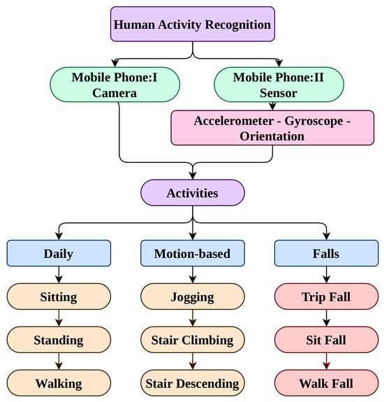
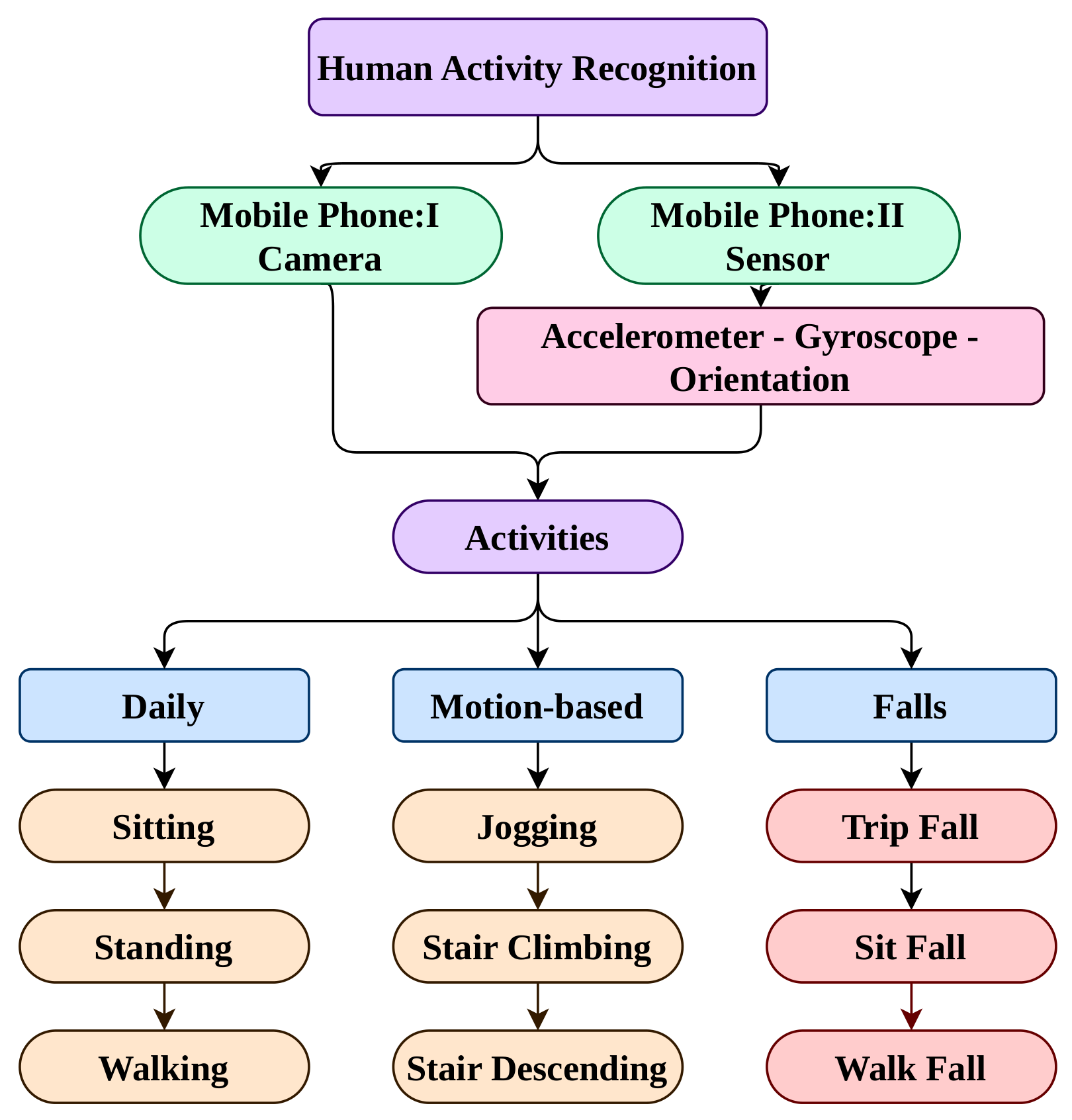
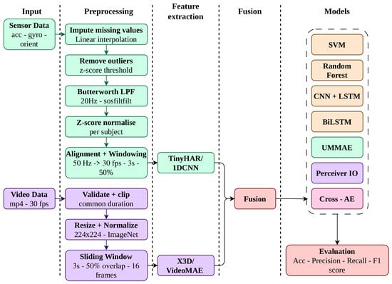
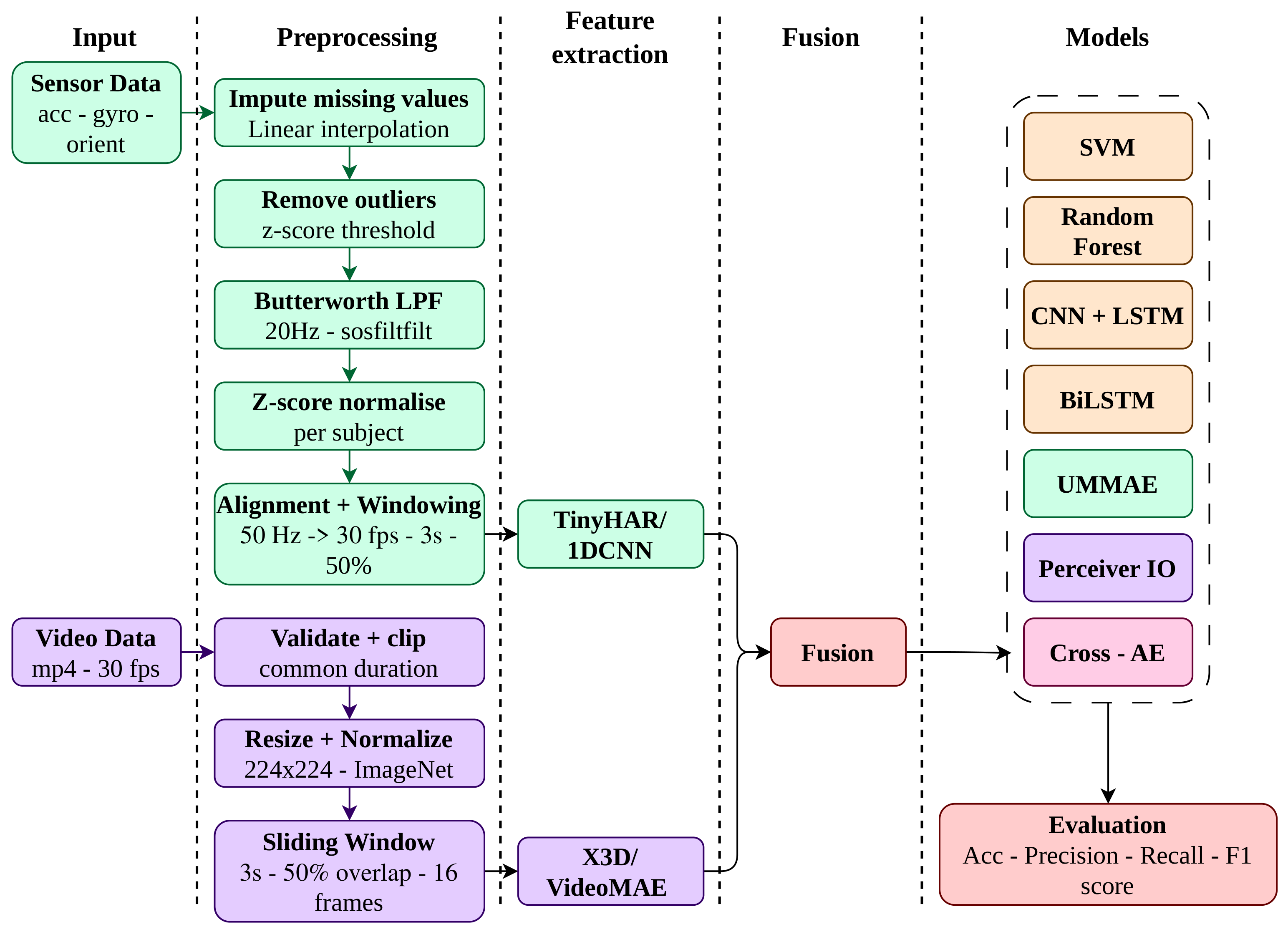
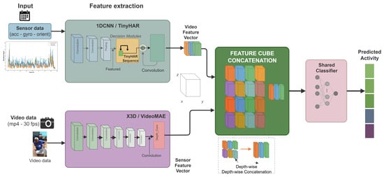
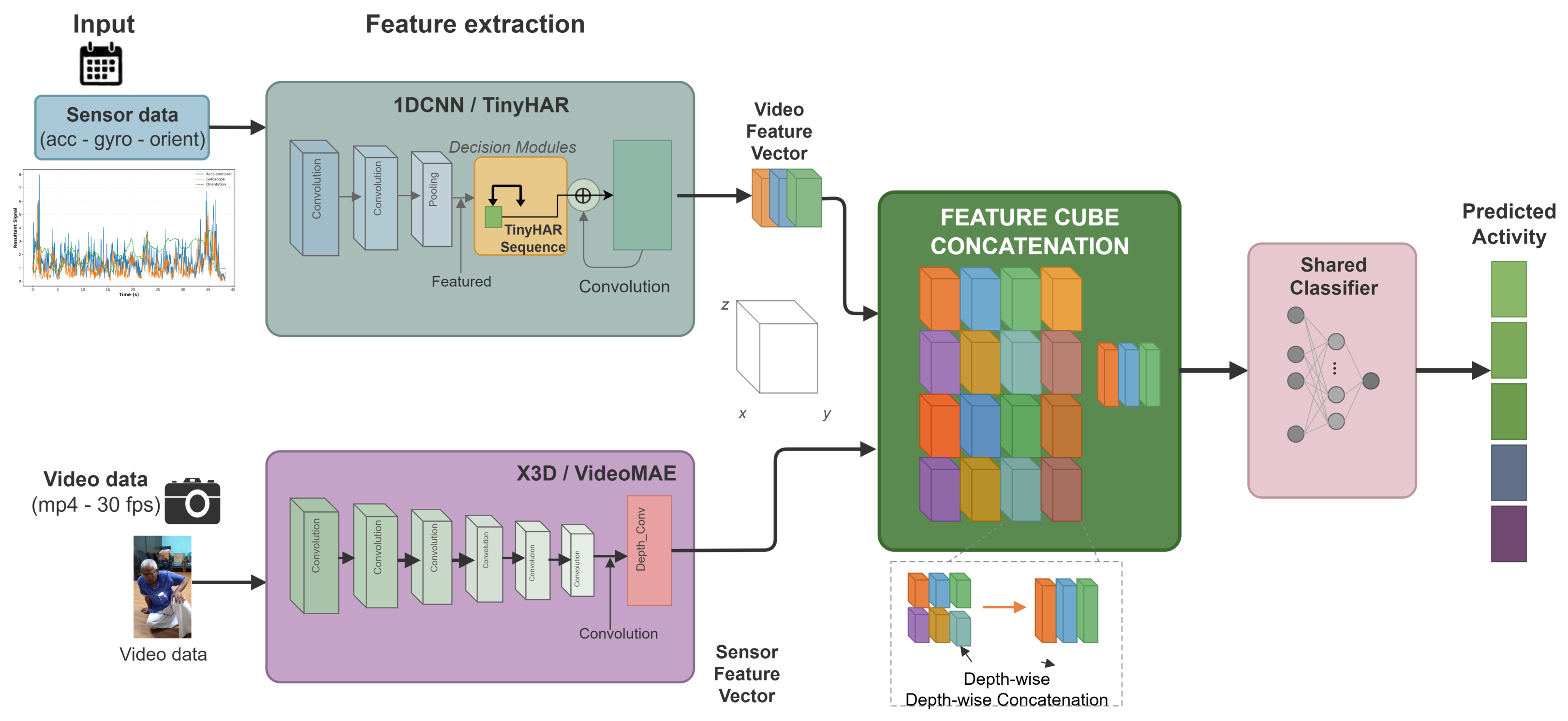
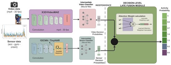
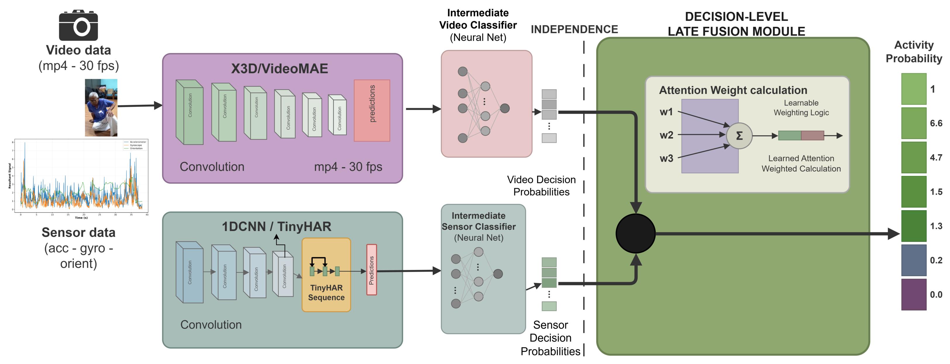
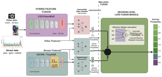
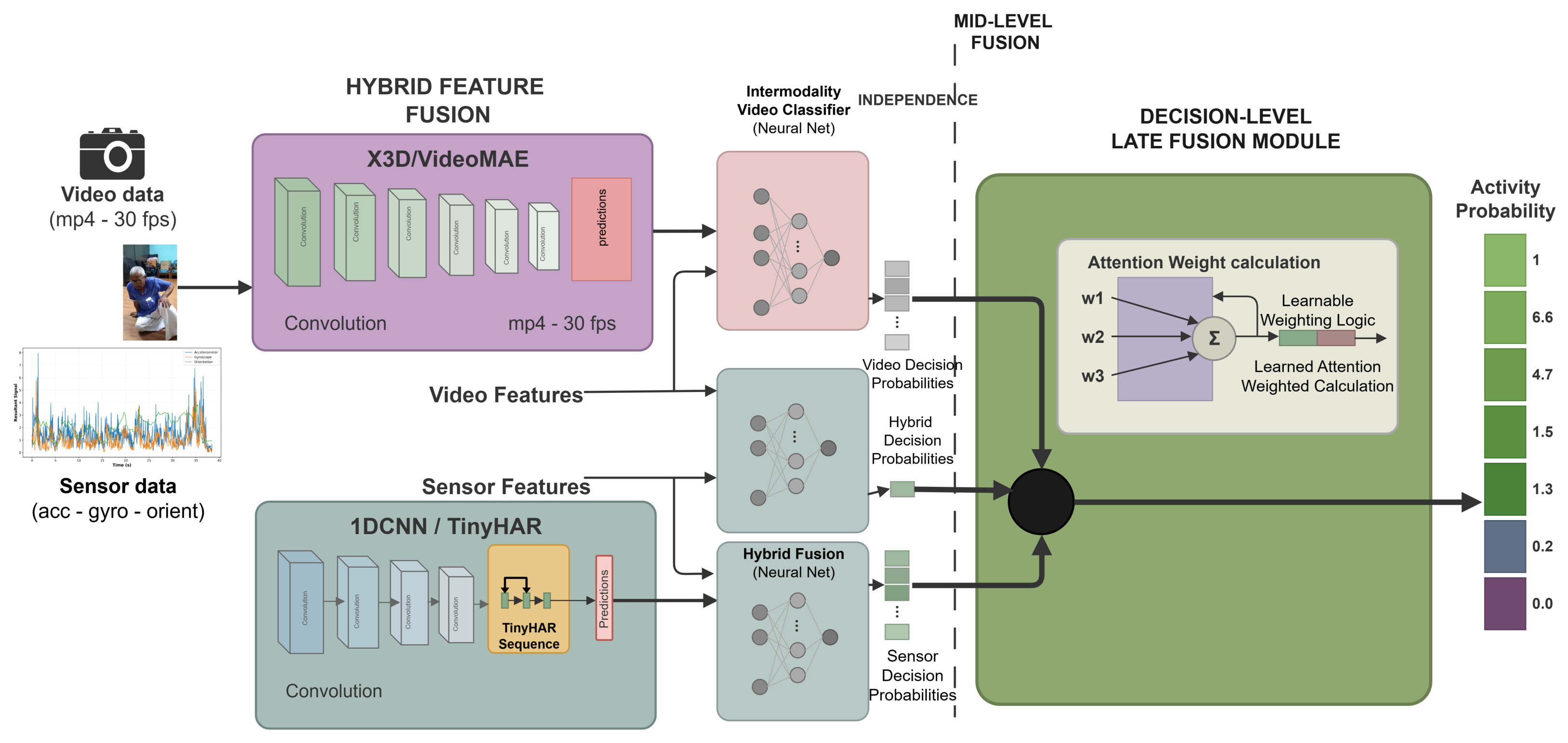
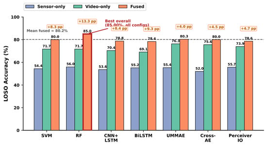
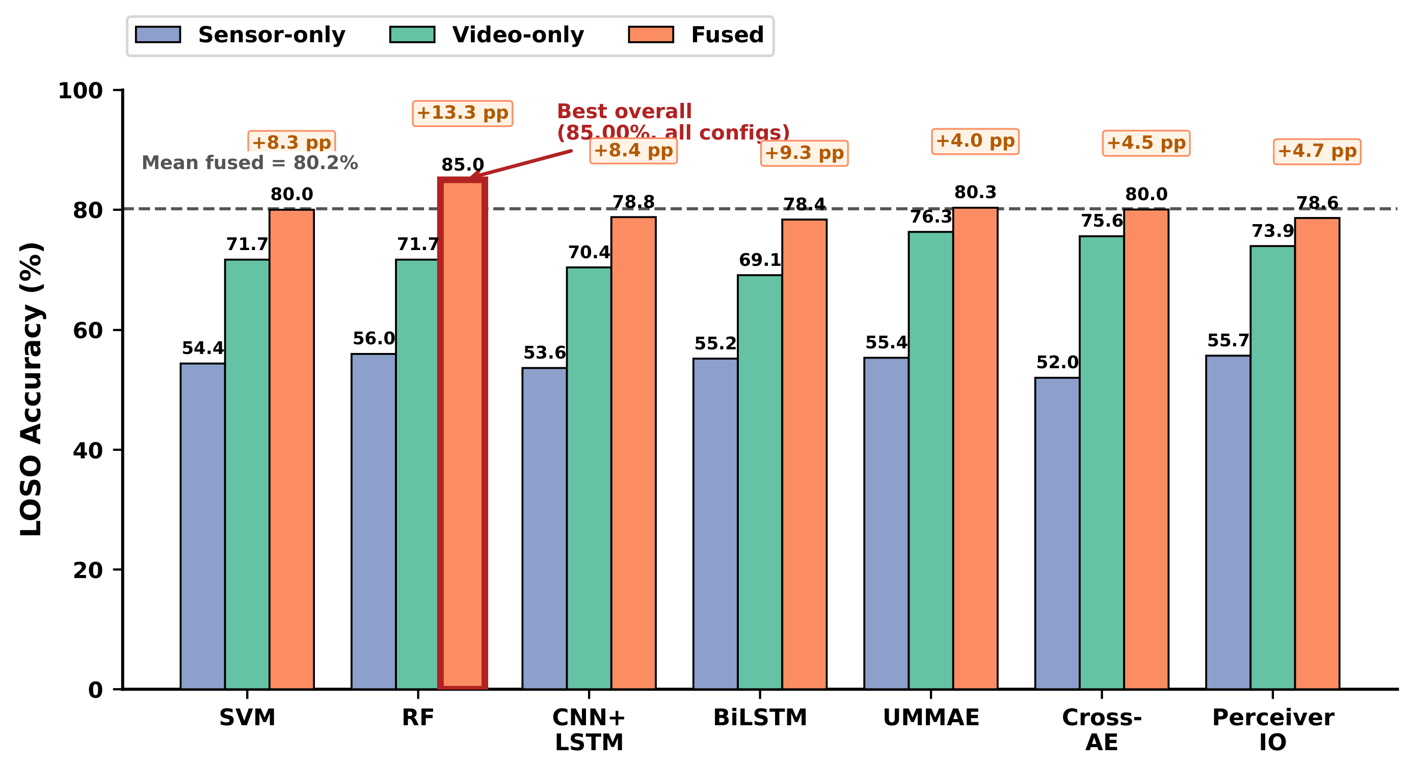
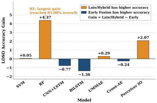
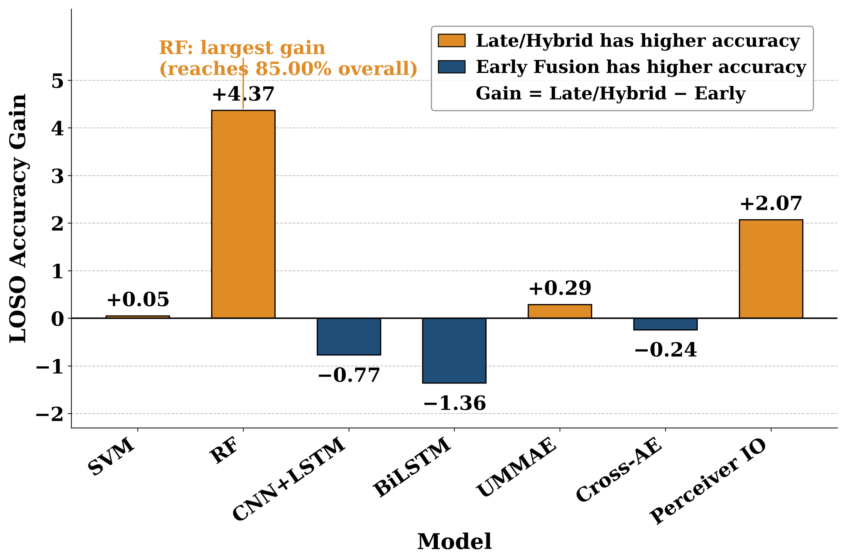
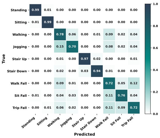
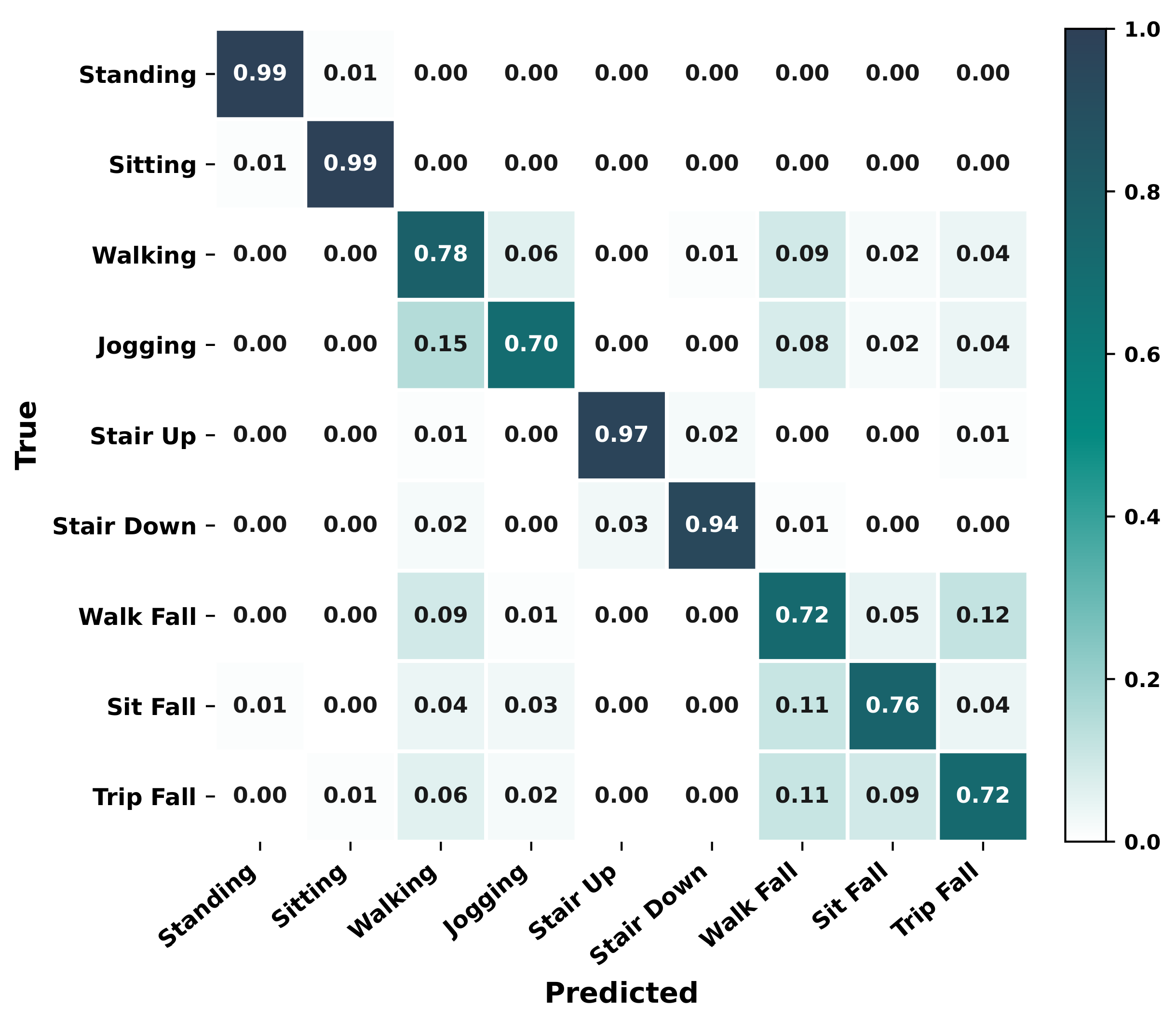
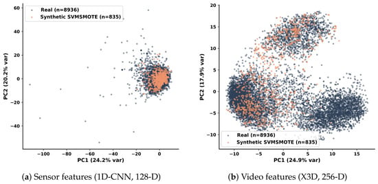
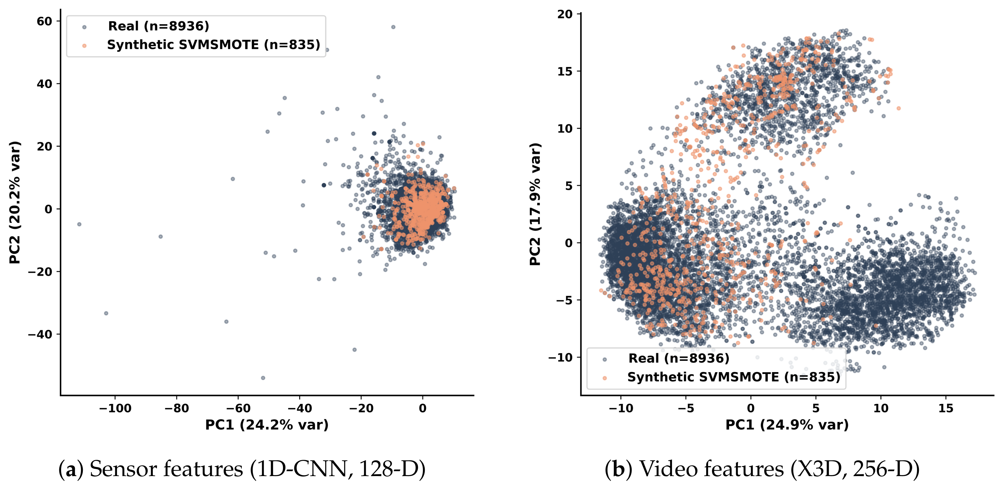
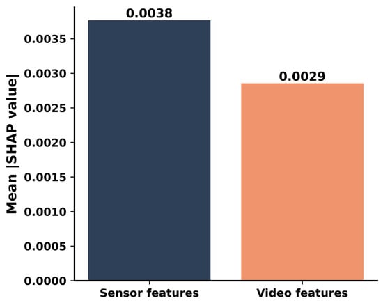
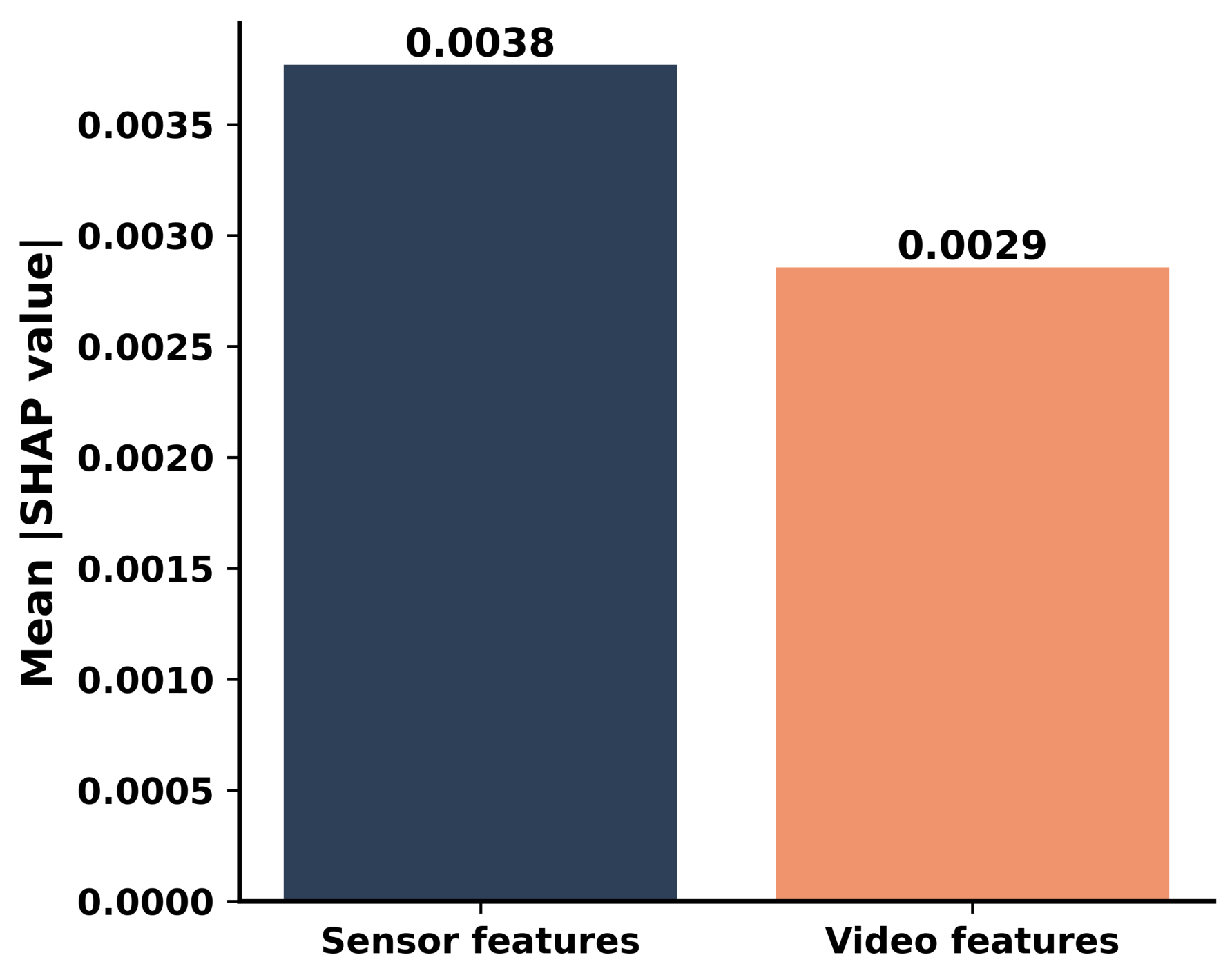
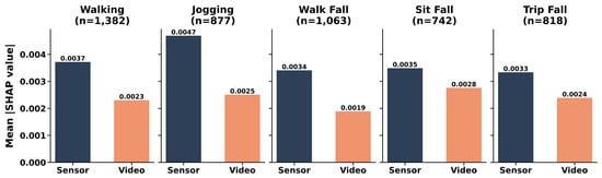
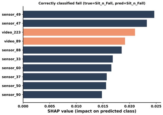
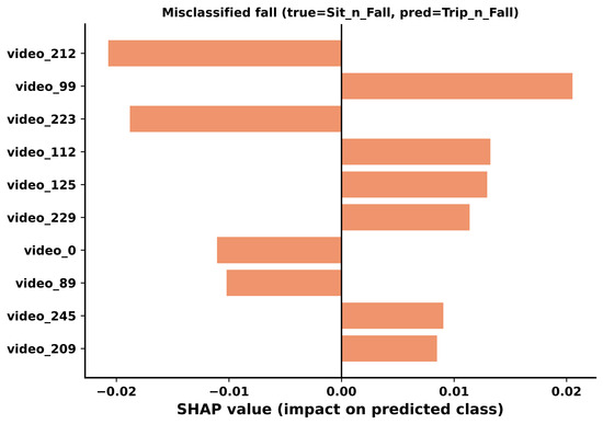
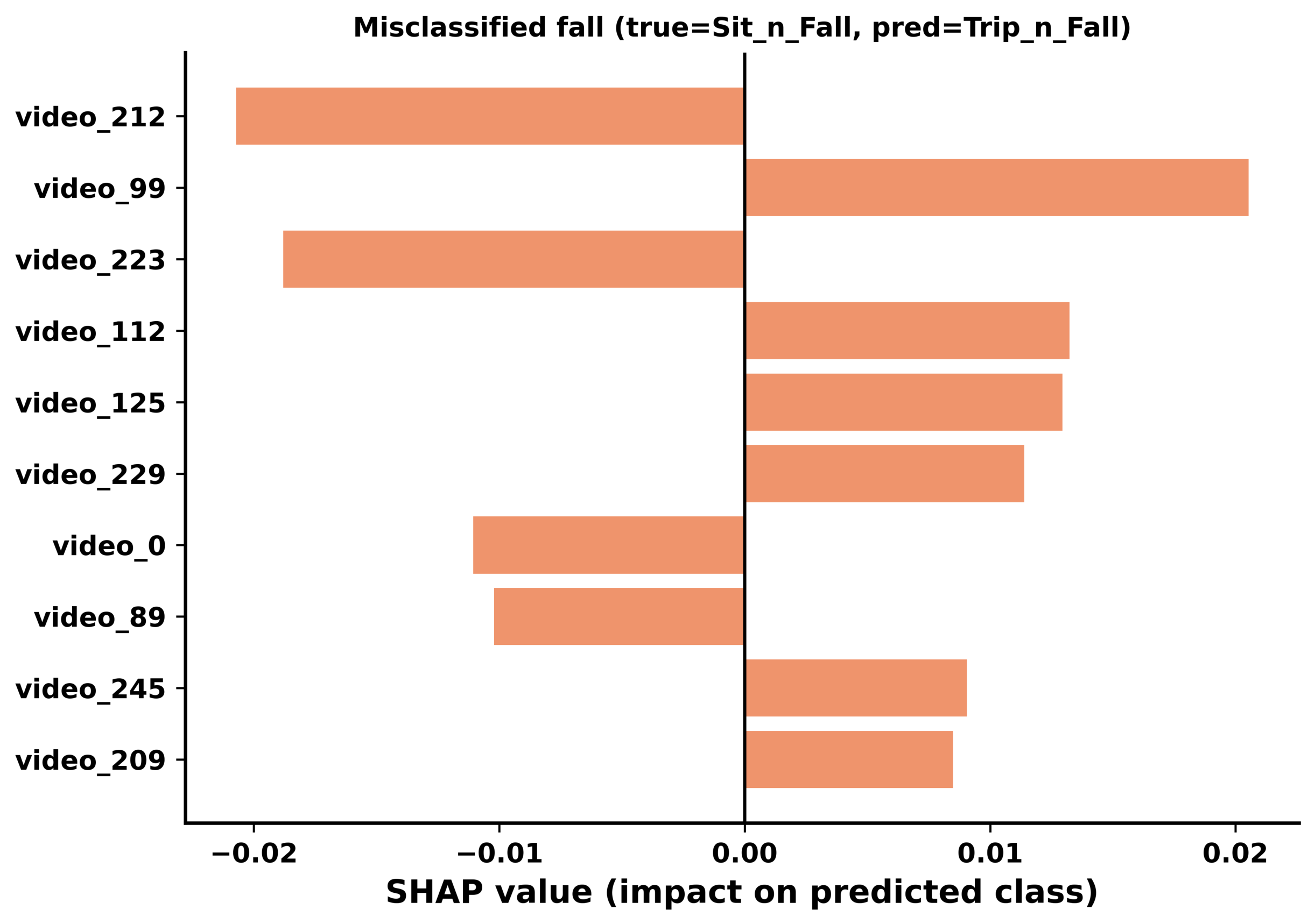
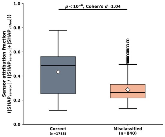
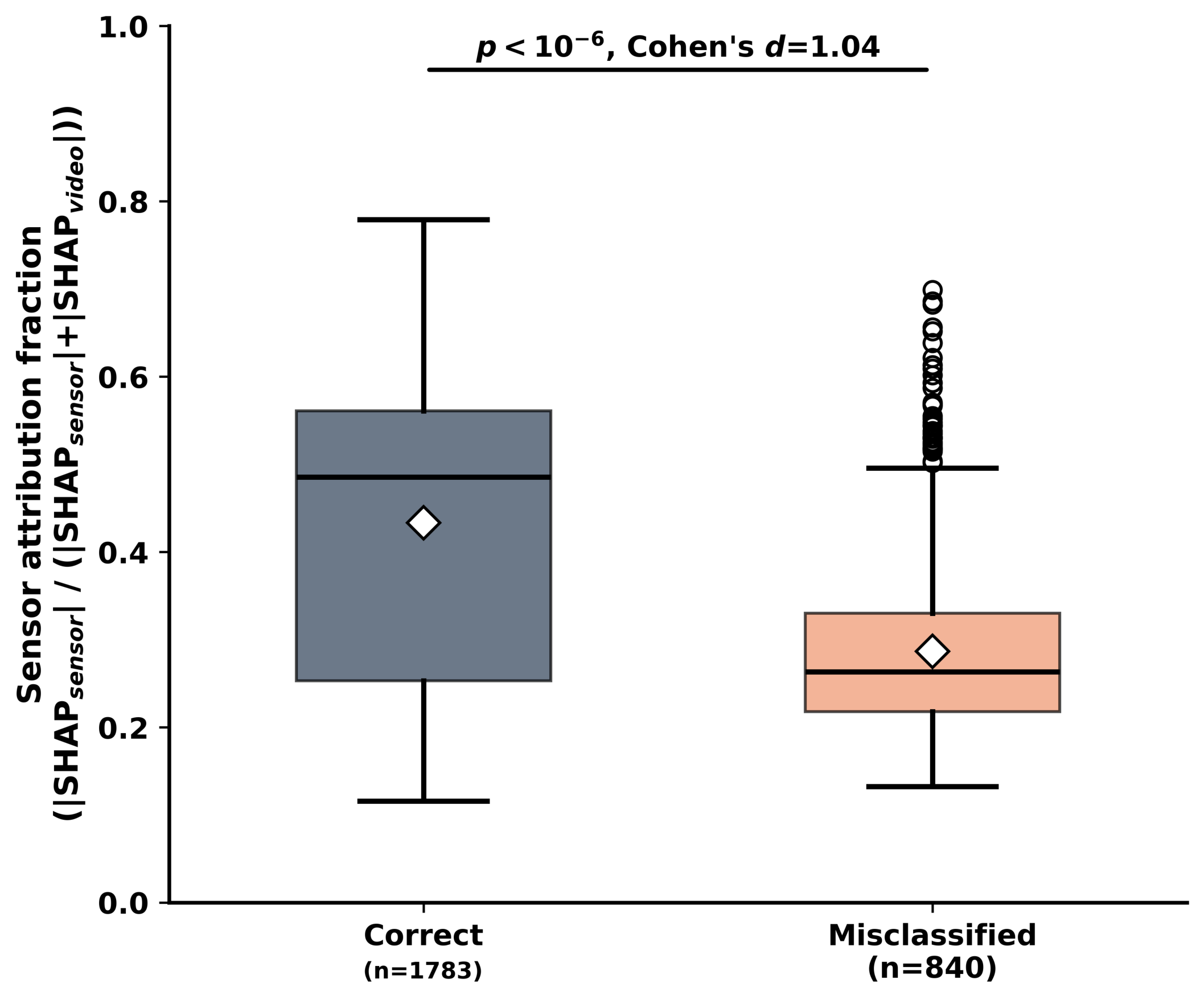
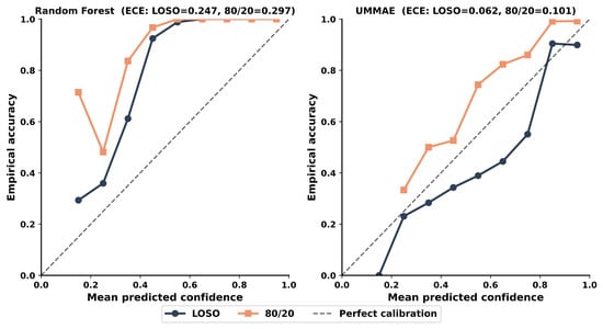
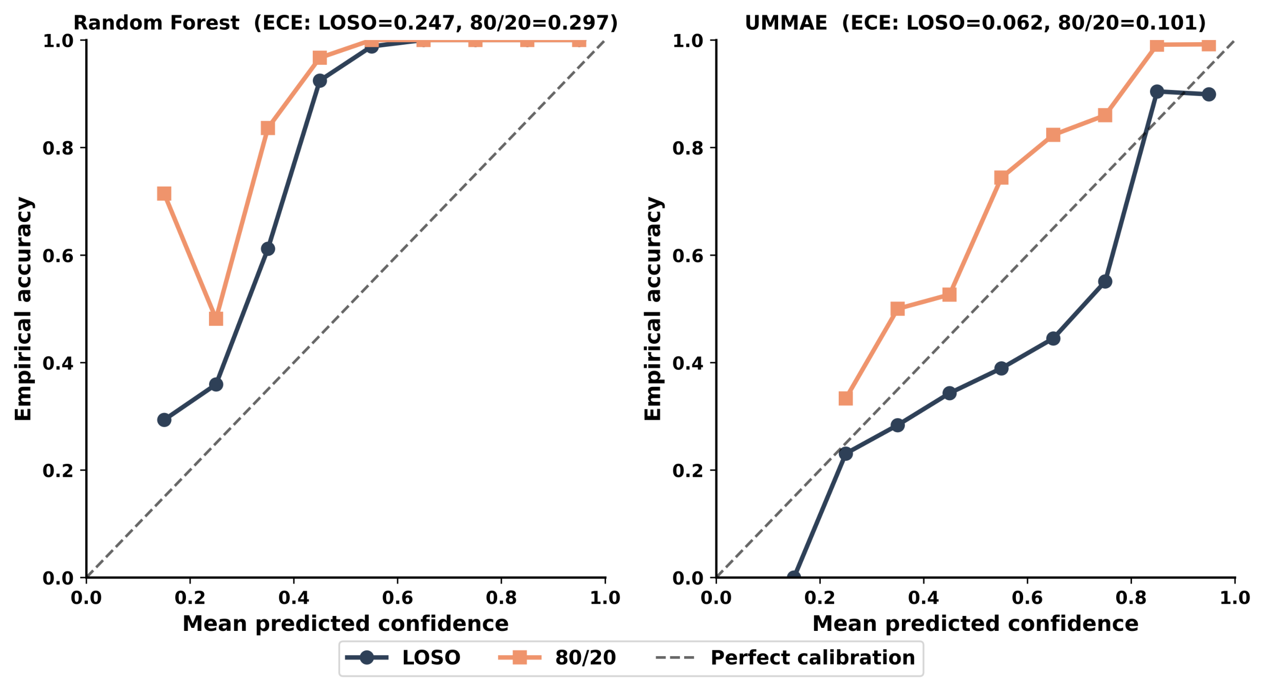

Disclaimer/Publisher’s Note: The statements, opinions and data contained in all publications are solely those of the individual author(s) and contributor(s) and not of MDPI and/or the editor(s). MDPI and/or the editor(s) disclaim responsibility for any injury to people or property resulting from any ideas, methods, instructions or products referred to in the content. |
© 2026 by the authors. Licensee MDPI, Basel, Switzerland. This article is an open access article distributed under the terms and conditions of the Creative Commons Attribution (CC BY) license.