Comparing Methods for Uncertainty Estimation of Paraganglioma Growth Predictions

Abstract

Background: Paragangliomas of the head and neck are rare, benign and indolent to slow-growing tumors. Not all tumors require immediate active intervention, and surveillance is a viable management strategy in a large proportion of cases. Treatment decisions are based on several tumor- and patient-related factors, with the tumor progression rate being a predominant determinant. Accurate prediction of tumor progression has the potential to significantly improve treatment decisions by helping to identify patients who are likely to require active treatment in the future. It furthermore enables better-informed timing for follow-up, allowing early intervention for those who will ultimately need it, and optimization of the use of resources (such as MRI scans). Crucial to this is having reliable estimates of the uncertainty associated with a future growth forecast, so that this can be taken into account in the decision-making process. Methods: For various tumor growth prediction models, two methods for uncertainty estimation were compared: a historical-based one and a Bayesian one. We also investigated how incorporating either tumor-specific or general estimates of auto-segmentation uncertainty impacts the results of growth prediction. The performance of the uncertainty estimates was examined both from a technical and a practical perspective. Study design: Method comparison study. Results: Data of 208 patients were used, comprising 311 paragangliomas and 1501 volume measurements, resulting in 2547 tumor growth predictions (a median of 10 predictions per tumor). As expected, the uncertainty increased with the length of the prediction horizon and decreased with the inclusion of more tumor measurement data in the prediction model. The historical method resulted in estimated confidence intervals where the actual value fell within the estimated 95% confidence interval 94% of the time. However, this method resulted in confidence intervals that were too wide to be clinically useful (often over 200% of the predicted volume), and showed poor ability to differentiate growing and stable tumors. The estimated confidence intervals of the Bayesian method were much narrower. However, the 95% credible intervals were too narrow, with the true tumor volume falling within them only 78% of the time, indicating underestimation of uncertainty and insufficient calibration. Despite this, the Bayesian method showed markedly better ability to distinguishing between growing and stable tumors, which has arguably the most practical value. When combining all growth models, the Bayesian method using tumor-specific auto-segmentation uncertainties resulted in an 86% correct classification of growing and non-growing tumors. Conclusions: Of the methods evaluated for predicting paraganglioma progression, the Bayesian method is the most useful in the considered context, because it shows the best ability to discriminate between growing and non-growing tumors. To determine how these methods could be used and what their value is for patients, they should be further evaluated in a clinical setting.

1. Introduction

Head and neck paragangliomas are rare tumors characterized by indolent to slow progression. Not all paragangliomas necessarily need active treatment. However, growing tumors may cause serious complaints, primarily involving hearing, balance and swallowing. Surveillance is therefore necessary, with regular MR imaging to evaluate tumor progression, as also concluded in a recent review study [1]. Unfortunately, active treatment modalities, i.e., surgery or radiotherapy, carry an inherent risk of cranial nerve damage that may result in complications very similar to those caused by the tumor itself. Therefore, making treatment decisions is difficult. Being able to make accurate predictions of tumor growth would be of great value when deciding which patients require active intervention in the near or more distant future, and to optimize the timing of active intervention when necessary [2,3]. Additionally, accurate growth prediction could improve follow-up timing and reduce the number of MR scans required for adequate monitoring.

Patients with head and neck paragangliomas often carry mutations in SDHA, SDHB, SDHC, or SDHD, and the specific mutation type may influence tumor growth behavior. However, this has not been observed or published in the past. In our cohort, SDHD was the most common mutation (55%). Tumors also occur at different anatomical sites, including the carotid body, vagal, jugular, and tympanic regions, which may further affect growth patterns.

In previous studies, we published a novel eXplainble Artifical Intelligence (XAI) technique that explicitly evaluated multiple growth curve models, to accommodate the possibility that different mutations or locations could result in distinct growth dynamics [4]. This AI technique identified three growth patterns that describe paraganglioma tumor growth well. These models are similar or equivalent to the Gompertz model, which is traditionally used to describe the growth of (cell) populations [5]. It reflects near-exponential growth initially, which eventually declines due to limited resources. Additionally, the Gompertz model, logistic model or related mathematical models are regularly used to model tumor growth [2,6,7]. While the different Gompertz patterns seem to fit the data well, no connection could be established between available patient data and the model that performs best for a given tumor.

In the current study, we investigate different ways to determine the uncertainty of these prediction models, in order to increase the usefulness and trustworthiness of the predictions. This study evaluates two methods for estimating uncertainty: a historical-based one and Bayesian one. The historical based method assumes that past errors are representative of future prediction errors, and is the standard statistical approach. However, Bayesian methods are also an established method for uncertainty prediction and have also been successfully applied for tumor growth uncertainty [6,7].

Other factors that may play a role in uncertainty prediction are volume measurement uncertainty and growth curve model uncertainty [8]. Therefore, we examine whether accounting for auto-segmentation uncertainty enhances the uncertainty estimates for growth prediction, since volume measurement is known to introduce some uncertainty. Additionally, we explore whether employing multiple models for predicting tumor growth can improve uncertainty estimation.

We compare how the two methods for uncertainty estimation perform from a technical perspective and a practical perspective. We also evaluate the effect of auto-segmentation uncertainty and using multiple models. Finally, we demonstrate how uncertainty information can be used to distinguish tumors that are very likely to grow from those that will remain stable in the future.

2. Materials and Methods

2.1. Tumor Volume Data

Patients with head and neck paragangliomas treated at the Leiden University Medical Center (Leiden, The Netherlands) were included in this study if at least three MRI scans were acquired for follow-up purposes between 2000 and 2020. We included 3D TOF gadolinium-enhanced MRI scans taken with a 1.5 T or a 3 T Philips Medical Systems scanner (Philips Medical Systems, Best, The Netherlands) with the following mode of MRI parameters: in-plane shape 256 × 256, number of slices 200, in-plane resolution 0.82 × 0.82 mm, and slice thickness 0.75 mm. Tumor volumes were measured using an AI-based segmentation model developed with nnU-Net [9], the performance of which has been shown to be on par with that of humans [10]. The resulting tumor volume was cross-referenced with the radiology report to exclude obvious segmentation errors.

2.2. Tumor Growth Models

Next, we used models generated by an AI algorithm to predict paraganglioma tumor growth [4]. To ensure physical plausibility, three constraints were applied: (1) the tumor has no significant volume at birth, (2) the predicted volume at age 100 must be smaller than 1500 mL (the largest observed tumor volume at our institution), and (3) tumor volume cannot decrease over time. Further details can be found in Appendix A.1.

The algorithm identified three distinct models for describing paraganglioma growth well:

$$\mathrm{model} 1={\displaystyle \frac{c_1}{e^{c_2\cdot t^{c_3}}}}$$

$$\mathrm{model} 2={\displaystyle \frac{c_1}{e^{c_2\cdot e^{c_3\cdot t}}}}$$

$$\mathrm{model} 3={\displaystyle \frac{c_1}{e^{c_2\cdot e^{c_3\cdot t^2}}}}$$

These growth models are similar or equivalent to the Gompertz model, which is traditionally used to describe growth of (cell) populations [5]. All models have an S-shaped curve, consistent with bi-phasic growth patterns: an initial phase of accelerating growth, followed by a phase of decelerating growth.

In these models, the coefficients c¹, c², and c³ are free variables and should be tuned for a specific tumor based on multiple tumor volume measurements at various patient ages (denoted as t in the models). Further details on how we tune these coefficients can be found in Appendix A.2.

2.3. Uncertainty Estimation Methods

To estimate the uncertainty of growth predictions, we considered two methods: a historical one and a Bayesian one. In the historical method it was assumed that past errors (i.e., deviations from the predictions coming from one of the above models) are representative of future prediction errors, providing the basis for an uncertainty estimate. No explicit modeling of the source of the errors was performed. In the Bayesian method it was assumed that uncertainty in growth predictions could primarily be attributed to the uncertainty associated with the estimation of the model’s coefficients.

To estimate the 95% confidence interval for a growth curve prediction using the historical method, we used the 2.5th and 97.5th percentiles of normalized historical errors from comparable tumor growth predictions. Errors were considered comparable when the prediction model was based on the same number of measurements to tune the model and the model predicted the same number of years ahead. The historical errors were normalized by tumor volume to account for differences in tumor size. This approach is the standard statistical method for uncertainty estimation, as it attempts to guarantee calibration by matching the empirical error distribution. However, it only works reliably if the historical data are representative of future predictions, meaning that sufficiently representative tumor measurements must be available for this method to perform properly.

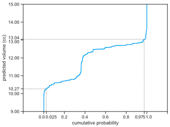
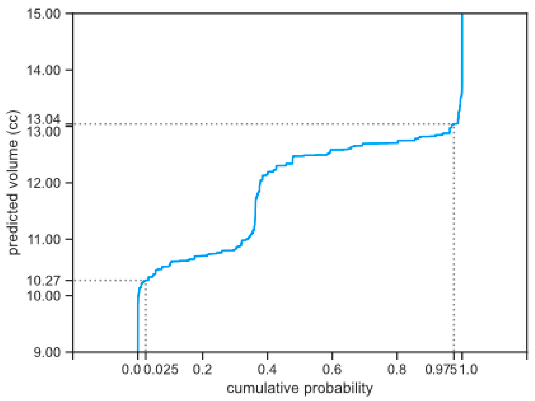
To calculate the estimate of the 95% confidence interval for a growth curve prediction using the Bayesian method, we used a Monte Carlo simulation [11]. The result of the simulation is a probability distribution rather than a single growth prediction [6,7]. From that distribution, we then derived the estimated 95% confidence interval, as illustrated in Figure 1. Further implementation details can be found in Appendix A.3.

Figure 1. Example of how the 95% confidence interval is derived from a cumulative probability distribution associated with the Bayesian method. In this example, the 95% confidence interval ranges from 10.27 to 13.04 cc.

In the Bayesian method, we factored in the uncertainty of the auto-segmentation. This was done by using a normal distribution estimate of tumor volume instead of a single value as volume measurement. We considered two ways to estimate this distribution: a tumor-specific estimate and a general estimate. Both ways rely on the ensemble method [12,13], which is typically useful for output generated by multiple models. Our segmentation model combined the output of five different models, as is standard for models trained with nnU-Net. From the output of these five models, we estimated the standard deviation of the normal distribution. More specifically, for the tumor-specific estimates, standard deviations of the tumor volume of the five different models were used. Further details can be found in Appendix A.4. For the general method, we used a standard deviation equal to the average of the standard deviations used in the tumor-specific estimates, expressed as a percentage of the mean tumor volume.

2.4. Evaluating Uncertainty Methods

When evaluating uncertainty estimates, two key factors are usually considered: sharpness and calibration [14]. Sharpness expresses how narrow the estimated confidence interval is, while calibration refers to how frequently observed values fall within the predicted interval. Ideally, estimated confidence intervals are both narrow and well-calibrated. However, there is often a trade-off between these two—improving one can worsen the other.

Some authors suggest offering multiple solutions with different trade-offs between calibration and sharpness for each individual tumor growth prediction [15]. However, this would either lead to an arbitrary selection or force users to make decisions for each tumor growth prediction, which could introduce additional complexity and bias (when it is difficult to determine the best solution, a user may choose the most convenient solution).

To address this, we compared this trade-off at the method level, rather than the individual tumor level. We assessed sharpness by measuring the median prediction interval width of the estimated 95% confidence interval, normalized by tumor volume, and evaluated calibration by tracking how often the observed value fell within the estimated 95% confidence interval.

While calibration and sharpness offer some insight into the usefulness and reliability of estimated confidence intervals, they do not always provide a complete picture. Calibration is typically averaged over multiple data points, which may not capture how well the intervals reflect reality. For example, a model with overly wide intervals for some datapoints and overly narrow intervals for others might still appear well-calibrated, but it may not accurately reflect real-world outcomes [16]. Moreover, a model that is well-calibrated but has overly wide intervals may not offer enough information for making treatment decisions.

To address this, we used an evaluation that is aimed at demonstrating usefulness in clinical practice. Specifically, we determined whether the uncertainty estimates could help distinguish between tumors that will grow, remain stable, or have uncertain outcomes.

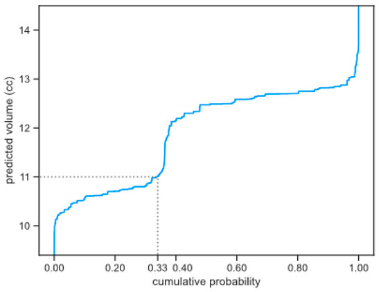
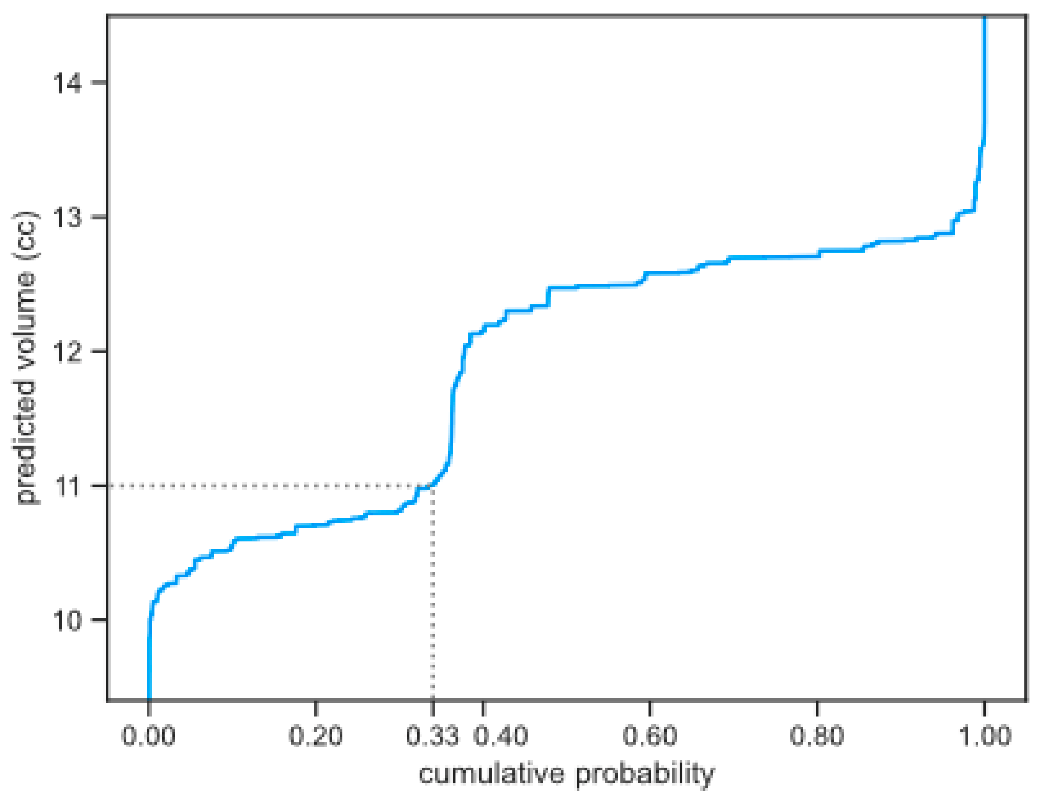
Tumors were classified as having a low (<5%) or high risk (>90%) for growth based on the predicted probability of growth using the cumulative probability distribution (as shown in Figure 2) and using a 20% volume increase as a threshold for growth (the 20% increase was based on [17], which was close to a more recent finding of an average smallest detectable difference of growth of 18% [8]). This classification could be determined for any future moment in time, but we determined the classification for the future moments in which we had available measurements, since it allowed us to determine the quality of the risk classifications. If the probability of a 20% increase in tumor volume at the next follow-up was estimated to be less than 5%, the tumor was classified as low risk, whereas if this probability was estimated to be more than 90%, the tumor was classified as high risk. Otherwise, the tumor remained unclassified. We evaluated how well these risk classifications aligned with the actual tumor growth, using the same 20% as a threshold [17].

Figure 2. Example of probability that the tumor will grow bigger than a certain volume, derived from the cumulative probability distribution. In this example the probability that the tumor grows above 11 cc is 67%.

To evaluate whether including multiple growth models as a form of uncertainty improved our risk classifications [12,13], we examined both the combined uncertainty of the three growth prediction models (later referred to as the combined models method) as well as their individual uncertainties. The risk classification of the combination of all growth prediction models was calculated by taking the lowest chance of growth when the minimum chance of growth of the three models was above 80%, and by taking the highest chance of growth when the maximum chance of growth of the three models was below 20%; otherwise, the average of the three prediction models was taken. This approach adopts a more conservative stance on risk classification than averaging the results of the three models by essentially looking at the worst case.

3. Results

We used data of 213 patients. Five patients were excluded because their volume measurements could not be matched with the radiology reports. In the remaining 208 patients, a total of 311 paragangliomas were detected. A total of 1515 tumor segmentations were available from these 311 tumors. Fourteen of those tumor segmentations were deemed inaccurate since they did not align with the tumor volume changes as described in the radiology reports, and were not included in the growth predictions. With the remaining 1501 tumor segmentations, we could study 2547 tumor growth predictions (a median of 10 predictions per tumor).

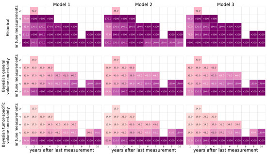
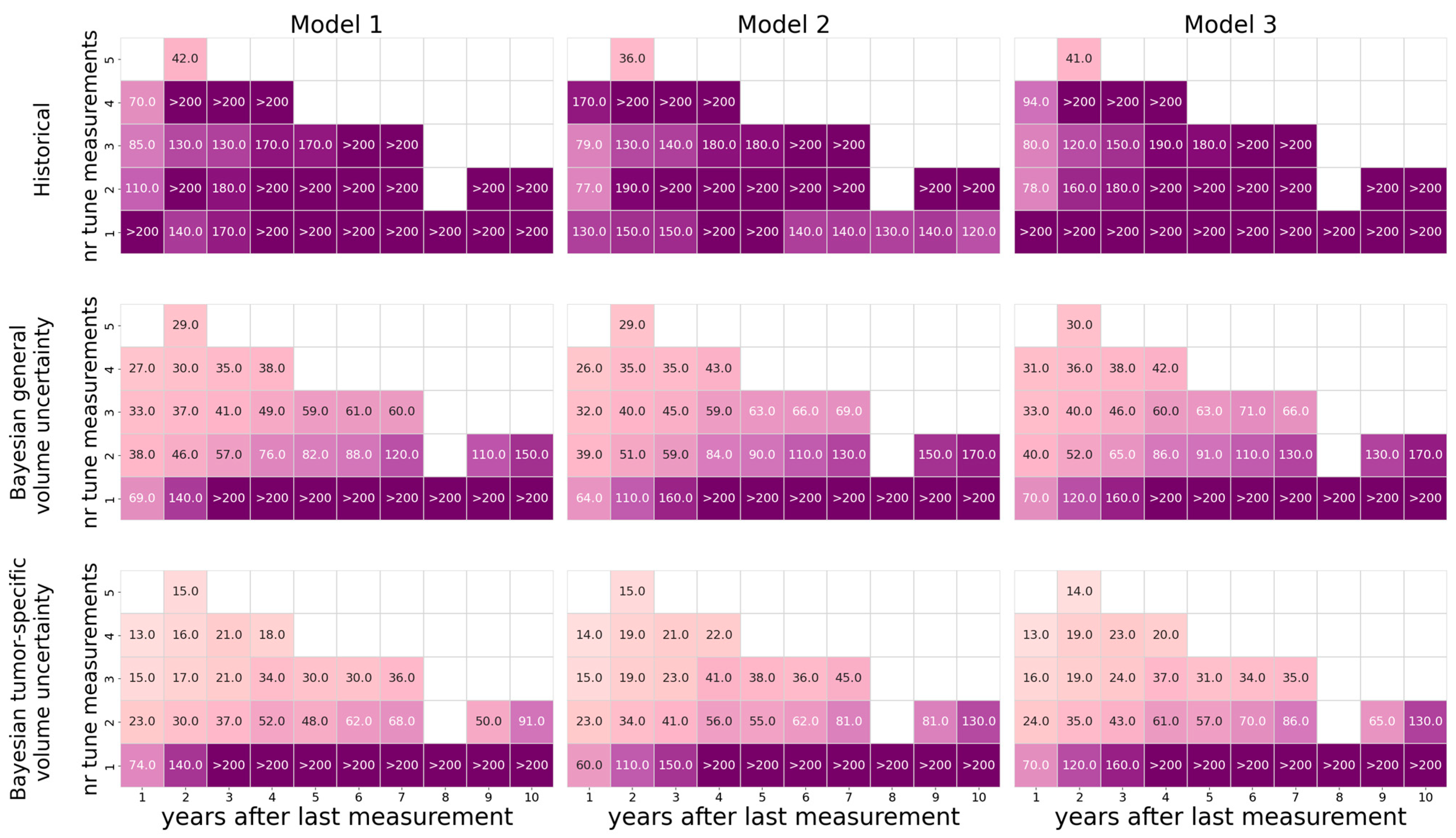
The sharpness of the estimated uncertainty is shown in Figure 3. As expected, the uncertainty increased with a decreasing number of measurements used to tune the coefficients, and with forecasts projected further in time. In line with this, most predictions based only on a single tumor volume measurement resulted in a 95% confidence interval that was bigger than the predicted volume itself, regardless of the method used. The historical method estimated large confidence intervals for all predictions, often surpassing 200%. The Bayesian method led to narrower estimations of the confidence intervals. Using tumor-specific estimations of auto-segmentation uncertainty generally narrowed the estimated confidence intervals. With respect to the estimated uncertainty, no relevant differences were observed between the three different growth models (comparing median differences between the models).

Figure 3. Median width of the estimated 95% confidence interval as percentage of the tumor volume. Darker colors indicate wider confidence intervals and, therefore, worse scores. For each method the three different growth models are compared. The impact of multiple measurements (vertical axis) and number of years to forecast (horizontal axis) are plotted, showing the best results for short-term predictions based on multiple historical measurements using the Bayesian method and tumor specific volume uncertainty.

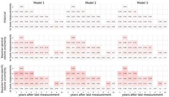
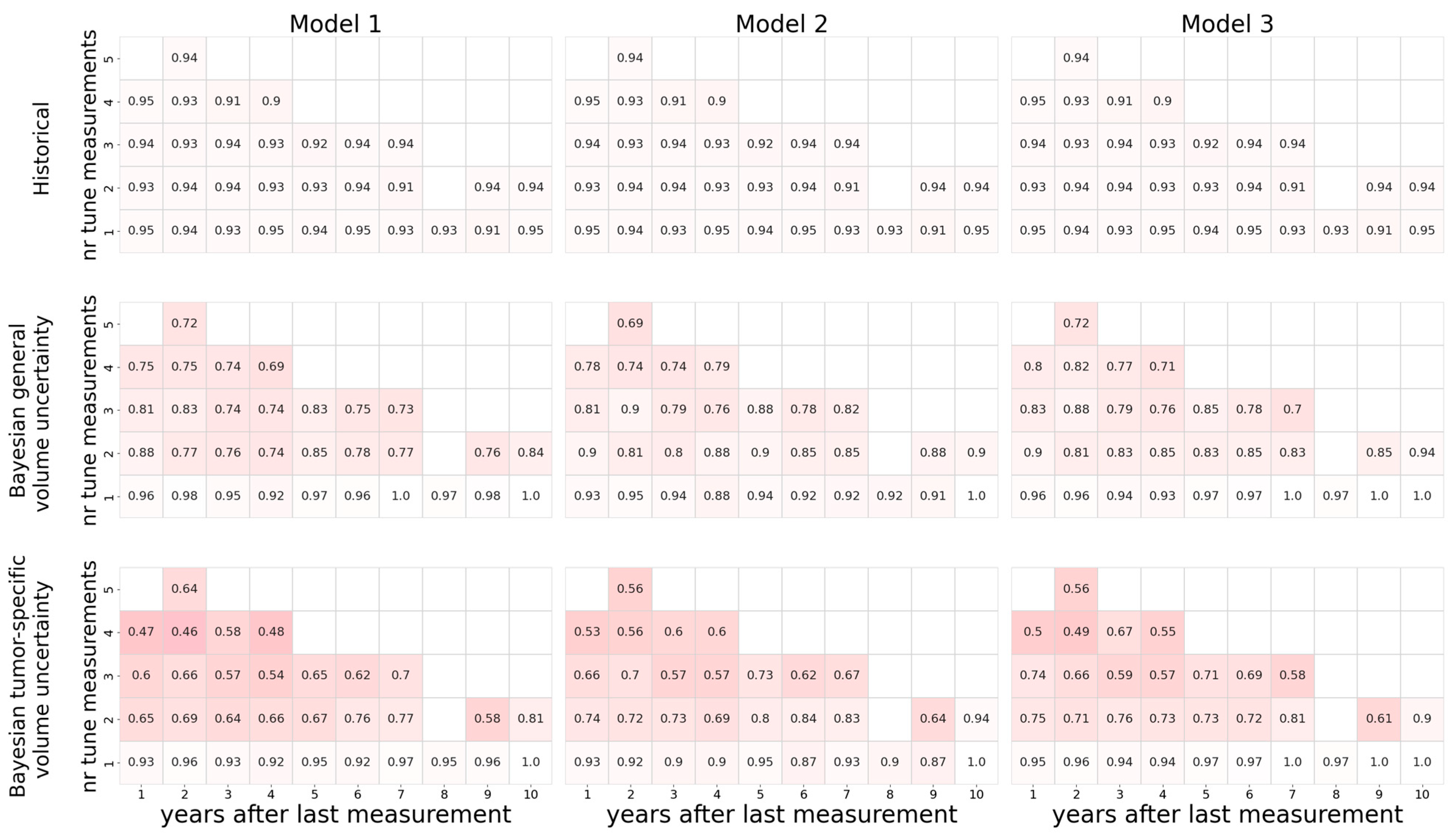
The calibration in terms of the proportion of predictions where the actual measurement fell within the predicted estimated 95% confidence interval is shown in Figure 4. As expected, this showed an inverse relation to the width of the estimated confidence intervals estimated and depicted in Figure 3. Across all predictions, the historical method’s 95% intervals contained the true volume approximately 94% of the time, which is close to the nominal level, whereas the Bayesian method’s 95% credible intervals contained the true volume only approximately 78% of the time, indicating the model’s under-calibration.

Figure 4. The fraction of prediction instances that fell within the estimated 95% confidence interval. Darker colors indicate lower fractions and, therefore, worse scores. For each method the three different growth models are compared. The impact of multiple measurements (vertical axis) and number of years to forecast (horizontal axis) are plotted, showing the best results for short-term predictions based on multiple historical measurements for the Historical method.

The historically generated uncertainty estimates did not reliably differentiate between tumors with a low (<5%) or high (>90%) risk of growth (Table 1). Bayesian derived estimates performed much better both using general volumetric or tumor-specific volumetric uncertainty, especially when the output of all three models was combined. Table 1 shows that the Bayesian method that used general volume auto-segmentation uncertainties performed better in the low-risk category (8.2% vs. 15.3% growth). The number of classified tumors, however, was much higher in the tumor-specific estimate, reducing the number of unclassified predictions from 2017 to 1746 (Table 2). The unclassified predictions were mainly based on one or two observed tumor volumes only, but represent the majority of predictions made. For the Bayesian method, the unclassified category consisted of 69% (without volume uncertainty) and 74% (with volume uncertainty) from predictions based on only one or two measurements. This is in line with our initial results that show that less available measurements increase uncertainty. As expected, using only one prior measurement yields very large uncertainty intervals (often >100% of the predicted volume), making those forecasts of limited practical value.

Table 1. Observed growth percentages for different risk classifications. These scores reflect how well the method and model were able to correctly classify the risk of growth. The better the risk classifications, the better the observed growth percentages aligned with them. Consequently, low growth percentages are desired in the low-risk category, and high growth percentages are desired in the high-risk category. The scores marked in bold are the best scores for that method.

Uncertainty Method	Model	Low Risk	Unclassified	High Risk
Historical	Model 1	41.7	58.5	58.5
	Model 2	60.0	58.5	43.8
	Model 3	50.0	58.5	55.0
	Models combined	45.0	58.6	43.8
Bayesian general volume uncertainty	Model 1	15.2	60.6	84.9
	Model 2	15.7	62.0	86.6
	Model 3	20.5	61.1	86.7
	Models combined	8.2	60.7	88.7
Bayesian tumor-specific uncertainty	Model 1	18.8	61.2	85.2
	Model 2	18.7	63.1	86.8
	Model 3	24.7	63.3	87.0
	Models combined	15.3	62.5	88.3

Table 2. Number of predictions within the different risk classifications (for the combined models).

Uncertainty Method	Low Risk	Unclassified	High Risk
Historical	20	2511	16
Bayesian general volume uncertainty	255	2017	275
Bayesian tumor-specific uncertainty	424	1746	377

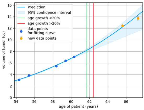
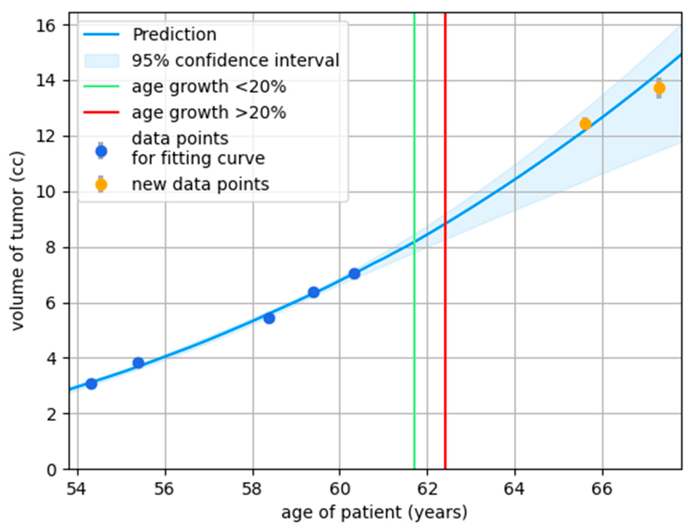
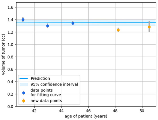
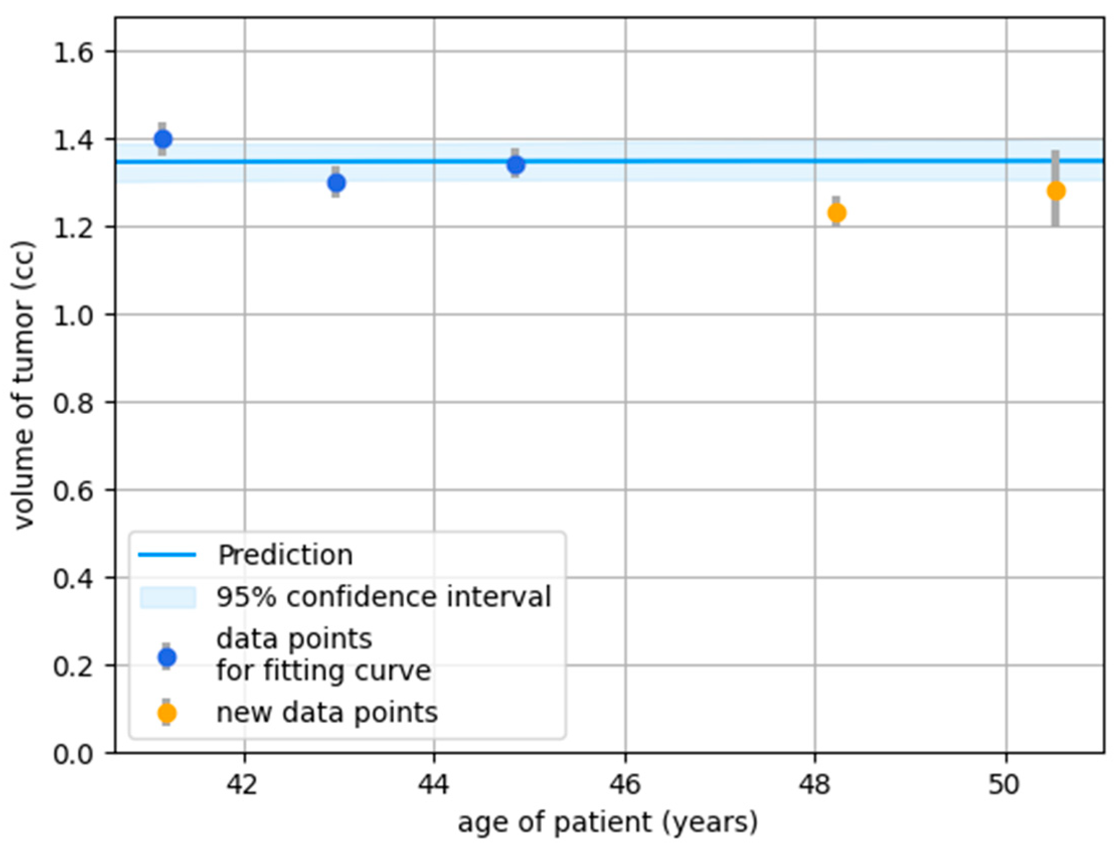
Figure 5 and Figure 6 are examples of how the presented methods could be useful in practice. Figure 5 shows a case of a clearly growing tumor, for which the prediction (of the Bayesian method) could have been a reason for earlier follow-up, or even a proposal for active treatment. In retrospect the tumor indeed showed significant growth. In contrast, the prediction (of the Bayesian method) of stable volume in the case depicted in Figure 6 could have led to less frequent imaging. In retrospect the tumor indeed did not grow for at least 5 years. In these scenarios, risk classifications can guide better-informed timing of follow-up measurements, avoiding assessment of the tumor before detectable growth has occurred (which could cause a false sense of security) or after excessive growth has occurred (which could lead to potentially irreversible complications).

Figure 5. Growth prediction with an estimated 95% confidence interval and age thresholds for risk classification: low-risk to unclassified (green) and unclassified to high-risk (red), based on data points (blue). The orange points represent future data that the model does not use. Grey bars indicate uncertainty in tumor-specific volume measurement. This example illustrates how short follow-ups comparing dimensional size (the standard clinical practice), rather than comparing total volume of the tumor (using volume measurement based on auto-segmentation), may falsely suggest no growth (ages 55.5, 59.5, and 60.5), leading to extended follow-up periods before growth is observed. Using the green and red lines to guide follow-up decisions could support a balanced measurement strategy, preventing both premature assessments (which may miss growth) and overly delayed ones (which may allow significant growth, potentially leading to irreversible complaints). At ages 59.5 and 60.5, no growth was detected, and follow-up time was extended, but following the growth predictions, different conclusions might have been reached, possibly leading to shorter follow-up intervals or consideration of active treatment.

Figure 6. Growth prediction with a 95% confidence based on data points (blue). The orange points represent future data that the prediction model does not use. Grey bars indicate uncertainty in tumor-specific volume measurement. The tumor is not predicted to grow the coming years. Based on this prediction, follow-up might have been scheduled after a 5-year interval (at age 50), measuring once instead of twice.

4. Discussion

The management of head and neck paragangliomas is challenging because of their uncertain behavior. Although other factors like symptoms, age, and co-morbidities also play an important role, treatment decisions largely depend on the expected growth of a paraganglioma. Accurate prediction of growth would therefore be enormously helpful in clinical decision-making. Discovering and fitting growth models as a means of making predictions, however, does not incorporate the uncertainty that is inherent to making predictions. Therefore, in this study, we aimed to compare different methods for estimating the uncertainty of the growth prediction.

The historical method resulted in estimated confidence intervals that were so high that they most likely are not useful in clinical practice. Both variants of the Bayesian method produced narrower confidence intervals, but were less favorable with regard to calibration. The historical method essentially ‘calibrates by construction’: it chooses interval bounds so that ~95% of past outcomes fall inside, but as a result it ignores case-specific information (i.e., the volume measurements of the tumor). This leads to very broad intervals in all cases. In contrast, the Bayesian method tailors the interval to each tumor’s data, which makes it narrower (more informative) but not as perfectly calibrated; in our results, only approximately 78% of true values fell within the nominal 95% interval. However, the Bayesian method was found to perform best at differentiating between tumors that will grow, those that will remain stable, and those with a more uncertain course. This type of prediction is likely a very helpful support in a clinical context.

Using multiple prediction models of growth simultaneously improved performance. We argue that tumor-specific auto-segmentation uncertainty is preferable over general uncertainty. Although the general method performed better in the low-risk category, the tumor-specific method was on par in the high-risk category and was able to classify 50% more predictions within their adequate risk categories. Multiple sources can introduce uncertainty [13,18], so combining uncertainty across the prediction models, coefficients, and volume measurements in the estimation method appears to make sense.

While we evaluated multiple models and also combinations of these models, some growth patterns might still not be covered. It very seldom occurs that a tumor drastically decreases in volume (in our dataset approximately 1% of tumors), which is not captured in any of the three models. Because only a handful of tumors show this behavior, it is more suitable for a case study than incorporating it into any (AI-based) growth model, merely because there are so little data on this phenomenon. Therefore, this scenario is not taken into account in our method. Additionally, in at least a few cases, the tumor seemed to be stable over some time and then seemed to resume progression later on. This pattern is also not covered by our three growth patterns. Further research should be performed to determine whether this pattern is valid, or whether (large) measurement errors could still play a role.

Furthermore, the Bayesian approach used here attributes growth prediction uncertainty mainly to uncertainty in the coefficients of the growth models, given the nnU-Net-derived tumor volume distributions. However, the resulting uncertainty bands are not the same as those obtained by repeatedly sampling tumor volumes from the nnU-Net-derived tumor volume distributions and refitting growth models. While both approaches may produce similar margins of uncertainty, the final shape of the growth curves for individual patients can differ. Studying the practical relevance of these differences remains a topic of interest for future work.

The auto-segmentation uncertainty estimates could be further developed and systematically evaluated. Although the volume measurement uncertainties of the segmentation model do show a slight improvement in performance in risk classification, our current study does not directly evaluate these uncertainty estimates. Furthermore, other sources of measurement variation such as geometric uncertainties of the MRI scan itself [19] or uncertainties related to variations in patient positioning are neither quantified nor taken into account. Further studies would be required to determine whether these or other potential sources of uncertainty have a significant impact on the prediction of paraganglioma growth. One particularly informative approach would be a repeat-scans study, in which a patient is scanned twice within a short interval. Although such studies are relatively expensive and logistically demanding, they are worth considering because they provide highly valuable information: the tumor itself does not change between scans, so any differences in measured volume must arise from measurement variability, whether segmentation-related or scanner-related. These overall variabilities could then be compared against the auto-segmentation uncertainty estimates. Additionally, these repeat-scan data could also help refine what should be considered a true growth threshold in clinical practice. Finally, this design would allow a direct comparison of measurement consistency between human delineation and model-based segmentation.

While consistency is the key factor for accurate assessment of growth over time, the measurement variability of absolute tumor volume (in terms of inter-observer variation) represents a clinically relevant source of uncertainty. To capture this type of variability, deep learning methods that explicitly model differences in annotations are required (e.g., [20]).

Before these uncertainty estimates can be used to guide clinical decisions, validation on an independent cohort is essential. In particular, to see if these findings can be generalized, further studies need to be performed on data from other centers. Furthermore, the practical use of risk categories requires careful evaluation, since even tumors classified as low-risk still showed a non-negligible chance of growth (approximately 15% in our data). Future studies should therefore assess how these predictions can best be incorporated into routine follow-up, for instance by determining how risk estimates could inform surveillance intervals or timing of intervention to improve on current outcomes.

5. Conclusions

We proposed two methods for adding uncertainty estimates to tumor growth predictions. In our retrospective analysis of head and neck paragangliomas, the Bayesian uncertainty approach provided the most useful predictions for growth, outperforming a historical-based method in terms of distinguishing between growing and non-growing tumors. This suggests that a Bayesian framework is preferable for this problem. Future (external) validation will be important to confirm these findings before clinical implementation. Furthermore, future studies should assess how these predictions can best be incorporated into routine follow-up. A logical next step would be to test the methods in a simulation of clinical decision-making, to assess the extent to which using these uncertainty estimates can safely reduce imaging frequency or prompt earlier interventions when needed.

Appendix A.1. Learning the Growth Prediction Models

The functional forms of the growth prediction models (i.e., including the free variables) were learned using a subset of the data, with the same settings and the same algorithm as described in [1]. The data set was split into two subsets. The first subset contained 80% of the tumors and was used during development of the models, also referred to as training data set. The other 20% was held to test the developed models. When splitting the data, we balanced the number of data points per tumor data set, such that each subset had a proportional number of measurements per data set. Additionally, if a patient had multiple tumors, all tumors were assigned the same split to keep the training and test sets independent. The subset used to learn the growth models comprised tumors in the training data set for which at least five measurements were available.

Appendix A.2. Fitting the Growth Prediction Models

When fitting the growth prediction models (i.e., tuning the free variables in the functional forms), we used fine-tuned coefficient ranges and constrained unlikely rapid growth. Specifically, the constraint prohibited more than a 10-fold volume increase in a year. Because we only know what is within the range of realistic growth when the tumor is at a human-detectable volume, this constraint was only considered when the tumor volume was at least 0.1 cc at the start of that year. To determine the fine-tuned coefficient ranges, for each coefficient we calculated the minimum and maximum values for that coefficient as observed for the fitted models in the training data set with at least five measurements (the same set as used for learning the growth prediction models). The maximum tumor volume coefficient c₁ was set to 1500 cc. Any other settings, as well as the algorithm used for fitting the models, were the same as in [3].

Appendix A.3. Implementation Details of the Bayesian Method

The Monte Carlo simulation of the Bayesian method started with an initial estimate of the distribution over the model coefficients, based on historical data from previous paraganglioma growth patterns. Next, the distribution over these coefficients was refined using the tumor volume measurements. This was achieved by repeatedly varying the initial coefficients and calculating the likelihood of the observed volume data for each variation, progressively updating the distribution to better match the tumor growth.

The pseudo-code of the method is shown as below. As a prior distribution over the coefficients, we employed a stratified Monte Carlo method [21], in which we sampled uniformly within each quartile of the fine-tuned coefficient ranges (as described in Appendix A.2), with each quartile sampled equally (Algorithm A1). This method provides a computationally efficient approach that better reflects the prior than a naive uniform or Gaussian approximation. With this prior, we reduced the likelihood of sampling invalid coefficient sets, which sped up the simulation by up to one order of magnitude compared to naive (min-max) uniform sampling.

Algorithm A1: SampleFromPrior (prior of model pm)
procedure: SampleFromPrior(pm)
1: l ← |pm|	(Get the number of coefficients of model m)
2: s ← []
3: for c from 1 to l do	(Separately sample for each coefficient c)
Q ← RandomChoice({Q0–0.25, Q0.25–0.5, Q0.5–0.75, Q0.75–1})	(Select quartile Q with 25% probability)
Qlower← LowerBound(pm[c], Q)
Qupper ← UpperBound(pm[c], Q)
s.append(RandomUniformSample(Qlower, Qupper))	(Sample prior between the bounds of quartile Q)
4: return s

Algorithm A2: GetPosterior (model m, prior of model pm, data of tumor d)
procedure: GetPosterior(m, pm, d)
1: l ← |pm|	(Get the number of coefficients of model m)
2: n ← 1
3: posterior ← EmptyMatrix(100,000, l+3)
4: while n ≤ 100,000 do	(Draw 100,000 valid samples of prior)
c ← SampleFromPrior(pm)	(Sample from the prior of the model)
if IsValid(c, m) then	(Check if the coefficients satisfy the constraints)
• posterior[n][0:l] ← [c1, c2, …, cl]	(Store coefficients)
• posterior[n][l+1] ← Likelihood(m, c, d)	(Store likelihood of coefficients)
• n ← n + 1
5: return posterior

Algorithm A3: GetPosteriorConfidenceInterval (model m, prior of model pm, data of tumor d, time for which to predict volume t)
procedure: GetPosteriorConfidenceInterval(m, pm, d, t)
1: l ← |pm|	(Get the number of coefficients of model m)
2: posterior ← GetPosterior(m, pm, d)
3: for n from 1 to 100,000 do
• posterior[n][l+2] ← CalculateOutcome(posterior[n], m, t)	(Get outcome of model at time t for all coefficients)
4: Sort(posterior, l+2)	(Sort posterior by outcome)
5: s ← sum(posterior[:][l+1])	(Compute sum of likelihoods s)
6: posterior[n][l] ← posterior[n][l]/s
7: for n from 2 to 100,000 do
• posterior[n][l+3] ← posterior[n][l+1]/s + posterior[n-1][l+1]	(Get cumulative sum of normalized likelihoods)
8: return GetQuantile(posterior, 0.025), GetQuantile(posterior, 0.975)	(Return 95% confidence interval for t)

To find the posterior distribution, we first sampled 100,000 valid coefficient sets from the prior distribution (Algorithm A2, step 4). This number of samples was experimentally determined to have a high likelihood of convergence. The coefficients are not valid when any of the four constraints are violated (Algorithm A2, step 4 ). Otherwise, the likelihood is calculated under the assumption of a normal distribution, with the following formula (Algorithm A2, step 4):

$$\prod _{i=0}^K{\displaystyle \frac{1.0}{{\sigma }_i\cdot \sqrt{\left(2\cdot \pi \right)}}}\times e^{-0.5\cdot {\left({\displaystyle \frac{\widehat{v_i}-{\mu }_i}{{\sigma }_i}}\right)}^2}$$

$\mu$ (the mean) and $\sigma$ (the standard deviation) are derived from the segmentation model, and $\widehat{v}$ is the volume predicted by the growth model for the specific set of coefficients for each of the K data points. Next, the cumulative probability distribution is calculated for a specific age t. Predictions for all 100,000 coefficient sets are made using the growth prediction model with t (Algorithm A3, step 3). These predictions are then sorted in ascending order (Algorithm A3, step 4). Next, the corresponding likelihoods of those predictions are normalized by the sum of all likelihoods, and their cumulative sum is computed to obtain the cumulative probability distribution (Algorithm A3, step 5–7). Based on the cumulative probability distribution, the 95% confidence interval is obtained (Algorithm A3, step 8).

Appendix A.4. Calculating the Tumor-Specific Standard Deviation

To calculate the tumor-specific standard deviation, we used the output of the five neural networks in the segmentation model obtained using nnU-net. Since multiple tumors could be present in one scan, it had to be decided which of the volume segmentations in the individual outputs referred to which tumor in the overall segmentation. We did so by matching each volume in the individual outputs to a volume in the overall segmentation. Each volume was only matched once (to the volume with the most overlap), and any volumes that did not overlap were left out. For any outliers in the standard deviations as ratio of the mean value, the individual volumes were inspected and if any outlier values were detected, the volumes causing the outlier value in the standard deviation were removed. This happened for 4 of the 1501 measurements.

References

- Graham, N.J.; Smith, J.D.; Else, T.; Basura, G.J. Paragangliomas of the head and neck: A contemporary review. Endocr. Oncol. 2022, 2, R153–R162. [Google Scholar] [CrossRef] [Scilit] [PubMed]
- Heesterman, B.; de Pont, L.; Verbist, B.; van der Mey, A.G.; Corssmit, E.P.M.; Hes, F.J.; van Benthem, P.P.G.; Jansen, J.C. Age and Tumor Volume Predict Growth of Carotid and Vagal Body Paragangliomas. J. Neurol. Surg. Part B Skull Base 2017, 78, 497–505. [Google Scholar] [CrossRef] [Scilit]
- Heesterman, B.; Bokhorst, J.; de Pont, L.; Verbist, B.M.; Bayley, J.-P.; van der Mey, A.G.L.; Corssmit, E.P.M.; Hes, F.J.; van Benthem, P.P.G.; Jansen, J.C. Mathematical Models for Tumor Growth and the Reduction of Overtreatment. J. Neurol. Surg. Part B Skull Base 2018, 80, 072–078. [Google Scholar] [CrossRef] [Scilit] [PubMed]
- Sijben, E.; Jansen, J.; Bosman, P.; Alderliesten, T. Function Class Learning with Genetic Programming: Towards Explainable Meta Learning for Tumor Growth Functionals. In Proceedings of the Genetic and Evolutionary Computation Conference, Melbourne, Australia, 14 July 2024; pp. 1354–1362. [Google Scholar] [CrossRef] [Scilit]
- Winsor, C.P. The Gompertz Curve as a Growth Curve. Proc. Natl. Acad. Sci. USA 1932, 18, 1–8. [Google Scholar] [CrossRef] [Scilit] [PubMed]
- Collis, J.; Connor, A.J.; Paczkowski, M.; Kannan, P.; Pitt-Francis, J.; Byrne, H.M.; Hubbard, M.E. Bayesian Calibration, Validation and Uncertainty Quantification for Predictive Modelling of Tumour Growth: A Tutorial. Bull. Math. Biol. 2017, 79, 939–974. [Google Scholar] [CrossRef] [Scilit] [PubMed]
- Dimitriou, N.M.; Demirag, E.; Strati, K.; Mitsis, G.D. A calibration and uncertainty quantification analysis of classical, fractional and multiscale logistic models of tumour growth. Comput. Methods Programs Biomed. 2024, 243, 107920. [Google Scholar] [CrossRef] [Scilit] [PubMed]
- Heesterman, B.; Verbist, B.; van der Mey, A.; Bayley, J.; Corssmit, E.P.M.; Hes, F.J.; Jansen, J.C. Measurement of head and neck paragangliomas: Is volumetric analysis worth the effort? A method comparison study. Clin. Otolaryngol. 2016, 41, 571–578. [Google Scholar] [CrossRef] [Scilit] [PubMed]
- Isensee, F.; Jaeger, P.F.; Kohl, S.A.A.; Petersen, J.; Maier-Hein, K.H. nnU-Net: A self-configuring method for deep learning-based biomedical image segmentation. Nat. Methods 2020, 18, 203–211. [Google Scholar] [CrossRef] [Scilit] [PubMed]
- Sijben, E.; Jansen, J.; de Ridder, M.; Bosman, P.; Alderliesten, T. Deep learning-based auto-segmentation of paraganglioma for growth monitoring. In Proceedings of the Medical Imaging 2024: Image Perception, Observer Performance, and Technology Assessment, San Diego, CA, USA, 2–7 February 2024; SPIE: Washington, DC, USA, 2024. [Google Scholar] [CrossRef] [Scilit]
- Mooney, C.Z. Monte Carlo Simulation; Sage Publications: London, UK, 1997. [Google Scholar]
- Lakshminarayanan, B.; Pritzel, A.; Blundell, C. Simple and scalable predictive uncertainty estimation using deep ensembles. In Proceedings of the 31st International Conference on Neural Information Processing Systems, Auckland, New Zealand, 2–6 December 2024; Curran Associates Inc.: New York, NY, USA, 2024; pp. 6405–6416. [Google Scholar]
- Werner, M.; Junginger, A.; Hennig, P.; Martius, G. Uncertainty in equation learning. In Proceedings of the Genetic and Evolutionary Computation Conference Companion, Boston, MA, USA, 9–13 July 2022; ACM Digital Library: Los Angeles, CA, USA, 2022; pp. 2298–2305. [Google Scholar] [CrossRef] [Scilit]
- Chung, Y.; Char, I.; Guo, H.; Schneider, J.; Neiswanger, W. Uncertainty Toolbox: An Open-Source Library for Assessing, Visualizing, and Improving Uncertainty Quantification. arXiv 2021. [Google Scholar] [CrossRef] [Scilit]
- Andreu-Vilarroig, C.; Ceberio, J.; Cortés, J.-C.; Fernández, F.; Hidalgo, J.I.; Villanueva, R.J. Evolutionary approach to model calibration with uncertainty. In Proceedings of the Genetic and Evolutionary Computation Conference Companion, Boston, MA, USA, 9–13 July 2022; ACM Digital Library: Los Angeles, CA, USA, 2022. [Google Scholar] [CrossRef] [Scilit]
- Sluijterman, L.; Cator, E.; Heskes, T. How to evaluate uncertainty estimates in machine learning for regression? Neural Netw. 2024, 173, 106203. [Google Scholar] [CrossRef] [Scilit] [PubMed]
- Jansen, J.C.; van den Berg, R.; Kuiper, A.; van der Mey, A.G.L.; Zwinderman, A.H.; Cornelisse, C.J. Estimation of growth rate in patients with head and neck paragangliomas influences the treatment proposal. Cancer 2000, 88, 2811–2816. [Google Scholar] [CrossRef] [PubMed]
- Gawlikowski, J.; Tassi, N.; Ali, M.; Lee, J.; Humt, M.; Feng, J.; Kruspe, A.; Triebel, R.; Jung, P.; Roscher, R.; et al. A survey of uncertainty in deep neural networks. Artif. Intell. Rev. 2023, 56, 1513–1589. [Google Scholar] [CrossRef] [Scilit]
- Weygand, J.; Fuller, C.D.; Ibbott, G.S.; Mohamed, A.S.; Ding, Y.; Yang, J.; Hwang, K.-P.; Wang, J. Spatial Precision in Magnetic Resonance Imaging–Guided Radiation Therapy: The Role of Geometric Distortion. Int. J. Radiat. Oncol. Biol. Phys. 2016, 95, 1304–1316. [Google Scholar] [CrossRef] [Scilit] [PubMed]
- Dushatskiy, A.; Lowe, G.; Bosman, P.A.; Alderliesten, T. Data variation-aware medical image segmentation. In Proceedings of the Medical Imaging 2022: Image Processing, San Diego, CA, USA, 20–24 February 2022; SPIE: Washington, DC, USA, 2022; Volume 12032, pp. 759–765. [Google Scholar]
- Kroese, D.P.; Taimre, T.; Botev, Z.I. Handbook of Monte Carlo Methods; John Wiley & Sons: Hoboken, NJ, USA, 2013. [Google Scholar]
Disclaimer/Publisher’s Note: The statements, opinions and data contained in all publications are solely those of the individual author(s) and contributor(s) and not of MDPI and/or the editor(s). MDPI and/or the editor(s) disclaim responsibility for any injury to people or property resulting from any ideas, methods, instructions or products referred to in the content. |
© 2026 by the authors. Licensee MDPI, Basel, Switzerland. This article is an open access article distributed under the terms and conditions of the Creative Commons Attribution (CC BY) license.