


Highlights
What are the main findings?
- The paper proposes a collection of parametric models that can be used to simulate the (range) performance of sensors employed in counter-drone systems (C-sUAS). These sensors are based on different technologies (electro-optics, thermal infrared, acoustics, radio frequency, radar, lidar).
- Standardised parameter values have been proposed for each model based on an extensive review of the literature using publicly available data or commercially marketed specifications. The proposed framework addresses the issue of malicious sUAS in its entirety, balancing complexity and usability across its various models. This overview of the problem provides a better understanding of the various factors affecting the performance of the sensors employed in C-sUAS systems.
What are the implications of the main findings?
- The parametric nature of the models enables adaptable scenario-based simulations under varying operational and environmental conditions, supporting mission planning, risk assessment, and large-scale system-level analyses. Therefore, the framework provides a practical compromise between simplified empirical approaches and highly detailed physics-based modelling.
- By enabling the use of default parameter values when detailed sensor specifications are unavailable, the framework also supports realistic multi-sensor and sensor-fusion studies in data-constrained environments.
Abstract
The primary objective of this document is to provide a structured reference for performance evaluation of the different sensor technologies that can be found in counter-drone systems. Standardised parametric models for the sensor(s), drone(s) and the external environment are proposed, with the aim of predicting sensor performance under real-world conditions in representative protective scenarios against hostile drones. In addition to defining these models, the document introduces a set of standardised reference parameter values to ensure consistency, comparability, and practical usability in cases where complete system data are unavailable. A set of clearly stated assumptions will therefore be formulated, dictating the boundary conditions for which the selected model can or cannot be used. The advantages of the parametric and standardised approach are numerous. For example, it makes it straightforward to compare the performance of different systems during a tender process, given that a set of common parameters must be known and provided (supplier data or standardised default values) for each system. This modelling approach also reduces the costs linked to practical field tests/deployment. Note that the focus is placed on developing simpler models to ensure ease of use and practical applicability, while maintaining an acceptable level of reliability and accuracy. The framework presented in this work is strictly oriented towards the defensive sensing function of C-sUAS systems and does not address effector design, kinetic engagement or offensive sUAS capabilities.
1. Introduction
Unmanned aircraft systems (UAS), commonly referred to as drones, are becoming prevalent in conflicts around the world [1,2,3,4,5], with NATO class 1 [6] small UAS (sUAS) playing a particularly prominent role for both state and non-state actors [7,8]. In response to the increasing use of sUAS, counter-small unmanned aircraft systems (C-sUAS), based on various technologies, have been developed [9,10,11] to defend against this new threat. These C-sUAS systems are used for security purposes, namely, to protect prisons [12], airports [13] and critical infrastructures [14] from attacks by malicious drones. Due to the limited number of standards regarding sensor performance evaluation, covering aspects such as effective detection range under operational conditions, data encoding schemes, and interoperability formats [15,16,17], the performance of these systems under operational conditions cannot be reliably predicted from supplier-provided specifications alone. As a result, it is difficult for the user to make a fair comparison of the claimed performances of different C-sUAS systems based solely on the technical specifications (i.e., the system datasheet) provided by the suppliers during a system selection process (i.e., procurement).
The main objective of this article is to provide a structured reference for evaluating the performance of various sensor technologies employed in C-sUAS systems, in order to facilitate decision-making and the selection of C-sUAS systems. The proposed framework covers six sensor modalities commonly employed in C-sUAS systems: electro-optics (EO), thermal infrared (TIR), acoustics (ACOU), radio frequency (RF), radar and lidar. By combining sensor performance prediction models with various environmental models, it is possible to simulate their actual performance (maximum detection range) once deployed in the field, taking into account a generic sUAS model. Each parameter used in the different models has been standardised according to specific criteria and is provided with a default value that can be used to run the model.
To this end, this article addresses three research questions:
- RQ1
- How can the actual field performance (maximum detection range) of C-sUAS sensors be simulated, considering the sUAS, the environmental conditions, and the different sensor modalities employed in C-sUAS systems, and how does each element of the scenario contribute to the final predicted performance?
- RQ2
- How can a generic sUAS and the external atmospheric factors (sun, rain, fog and wind) affecting sensor performance each be captured through standardised parametric models, with default values tied to identifiable input conditions?
- RQ3
- How can the detection performance of each sensor modality (electro-optics, thermal infrared, acoustics, radio frequency, radar and lidar) be modelled, and how can the influence of those environmental conditions be represented through modality-specific loss models?
The remainder of the article is organised so as to answer these questions. Section 2 introduces the parametric sUAS model, with a default configuration derived from the DJI Mini 4 Pro. Section 3 defines the parametric models for the external atmospheric factors and their condition-dependent default values. Section 4 presents the per-modality detection and loss models used to evaluate the detection performance of sensors in C-sUAS systems, together with a sensitivity analysis of the default parameter values (Section 4.9). Together, these elements support the simulation of the field performance of C-sUAS sensors and the contribution analysis of each element present in the scenario.
1.1. Standardisation Effort
Effectively addressing this issue requires the development of a comprehensive framework dedicated to standardising all elements involved in a typical C-sUAS scenario. Within this framework, several components must be considered. First, it requires the development and formalisation of a parametric model capable of accurately representing the diverse configurations and behaviours encountered in typical C-sUAS scenarios. Such a model must be accompanied by clearly defined assumptions and boundary conditions, specifying the context and limitations under which the model remains valid and applicable. Additionally, the framework includes a set of standardised reference values and explicitly defined default parameter values, proposed in this work, to support performance evaluation in situations where complete system specifications are unavailable (a common challenge in operational environments). These default values constitute a practical contribution of this article, enabling consistent and reproducible assessments across C-sUAS systems. A key contribution of this work is therefore the formal definition and provision of such default parameter values within a coherent parametric modelling framework. While a few isolated efforts exist—such as [18,19], which define the nominal range performance for thermal imaging systems and test strategies with performance metrics to quantify the capabilities of different C-sUAS systems—these efforts fall short of offering the comprehensive, integrated approach required to ensure interoperability, consistency, and reliability across the full spectrum of C-sUAS activities. A standardisation framework is built on the following elements:
- 1.
- Standardised parametric modelling establishes a scenario-driven approach that incorporates drone characteristics, defines key system parameters, and ensures interoperability with existing modelling and simulation tools.
- 2.
- Operational constraints and boundary conditions define the practical limitations of deployment, including sensor placement and mobility, terrain and line of sight delimitations, environmental conditions, and temporal dynamics such as communication and latency.
- 3.
- Sensor modality-specific standards integration builds upon existing Standardisation agreements (STANAGs) such as STANAG 4347 [18] and STANAG 4348 [20] to promote consistency and harmonisation in performance metrics across different sensing technologies.
- 4.
- Reference values and scenarios provide canonical threat profiles and standardised parameters for performance evaluation, supported by baseline configurations reflecting representative operational contexts.
1.2. Sensors Goal Within DTIM Workflow
While this document focuses on modelling sensor performance, consideration of the broader C-sUAS context, including the interplay of sensors, effectors, drones, and the environment, remains essential. Because of their strong interdependence with sensing, related aspects of drones and the environment are briefly examined in Section 2 and Section 3, respectively. The proposed sensor models, presented in Section 4, can be integrated within the variety of existing detection-to-mitigation frameworks [21,22]. This manuscript adopts the detection, tracking, identification and mitigation (DTIM) processing chain approach, structured around four main steps. These four main steps, together with the transitions linking them, are illustrated in Figure 1.
Figure 1.
The DTIM processing chain represents the main tasks managed by the sensors and effectors under the control of the C2 module in C-sUAS systems.
- 1.
- Detection (D): It relates to the fact that something has entered the area monitored by the C-sUAS system. At this stage, the system is able to attribute a category to the detected object such as sUAS, birds or insects.
- 2.
- Tracking (T): It refers to the action of keeping in memory an object’s movement over time. Prioritisation rules on objects to follow and track are therefore implemented in the core of the Command and Control (C2) module to ensure the strategy to adapt in scenarios involving multiple sUAS.
- 3.
- Identification (I): It refers to the extraction and analysis of the main features of the tracked sUAS. At this stage, the system is clearly able to distinguish and assign a class to each detected sUAS (e.g., DJI Mavic 2, DJI Phantom 4, Parrot Anafi, …) as well as determine its side (i.e., cooperative vs. non-cooperative). Crucially, this identification step relies on the use of an external database in most cases.
- 4.
- Mitigation (M): It relates to the physical interception of the sUAS platform, which falls outside the scope of this work.
2. Drone Modelling
This section addresses the first part of RQ2 by defining a generic, parametric sUAS model together with a standardised default configuration derived from the DJI Mini 4 Pro.
The main objective of this section is to introduce parametric models for the malicious sUAS. These models are required to balance fidelity in representing sUAS signatures with generality that ensures independence from specific sUAS platform. Characterising these signatures provides the basis for evaluating the detectability of the target and, by extension, the performance of C-sUAS systems during the design or evaluation of a given defence system.
Section 2.1 first provides a classification of sUAS that characterises the types of platforms considered in this study. Section 2.2 then uses this classification to highlight the main reasons why such platforms are challenging for current C-sUAS systems. Finally, Section 2.3 derives the corresponding sUAS signature models.
2.1. Drone Classification
In 2024, the multirotor and fixed wing drone markets were valued at approximately $4.1 billion and $21.08 billion, respectively. Projections indicated that these markets are expected to expand to $9.79 billion by 2029 and $170.95 billion by 2034 [23,24]. Given the diversity of available sUAS models, this paper covers only a portion of them. From all the classification schemes proposed for UAS classification [25,26], the NATO classification framework [6] has been selected. The sUAS considered in this manuscript fall within class 1, specifically the micro and mini categories, whose main characteristics are summarised in Table 1.
Table 1.
Table containing the main characteristics of the Mini and Micro sUAS category, adapted from [6].
2.2. Drone Challenges
The mini and micro sUAS categories, as defined in Section 2.1, represent low, small and slow aerial drones that pose specific challenges for C-sUAS systems [27,28]. Due to their low operating altitudes (up to 3000 feet above ground level (AGL)), the detection systems require sensors to monitor airspace close to the ground, where significant environmental clutter can degrade detection performance. Their reduced physical dimension, compared to conventional airspace systems (manned aircraft for instance), further complicate detection, as sensors must discriminate these small drones from background noise across multiple spectral domains without significantly increasing the false alarm rate (FAR). Finally, the relatively slow velocities of mini and micro sUAS, with the capability of hovering in static positions, create additional detection difficulties, as such sUAS can seamlessly blend into the surrounding environment and thus remain indistinguishable to C-sUAS systems.
2.3. Drone Signature
This section introduces the modelling parameters required to simulate a realistic mini or micro sUAS. For each sensing modality, the characteristic signature of a generic sUAS is first modelled independently, with its properties expressed through specific parameters. These per-sensor parameters are compiled into reference tables at the end of each subsection for clarity. Once all individual signatures have been established, they are all combined to form a complete signature for a generic sUAS. This unified signature encapsulates all relevant parameters, enabling the generation of drone models that can interact seamlessly with any sensor described in Section 4. The number, type and fidelity of these parameters scale with the complexity of the sensor model used in conjunction: a deliberate trade-off privileges practical implementability over exhaustive physical fidelity so that the sUAS model supports end-to-end DTIM processing chain simulation while yielding relevant performance predictions.
2.3.1. Electro-Optics Signature
The term electro-optics (EO) encompasses the visible (VIS), near infrared (NIR), and short-wave infrared (SWIR) spectral domains [29]. Within these domains, the detection of a sUAS corresponds to an object detection task, a problem that has been well studied in the computer vision and pattern recognition communities [30,31,32,33]. In this context, geometric features such as size, shape and orientation directly determine its visibility to EO sensors. To that extent, the parameter PCS, projected cross-section, is introduced. This parameter refers to the silhouette that a 3D object would cast onto a perpendicular plane to a given direction (i.e., direction of incoming radiation). The transformation produces a two-dimensional projection characterised by horizontal and vertical dimensions. Within this projected cross-section, another key parameter is the critical dimension , which represents the effective size of a sUAS as seen on the sensor plane. Several methods exist to compute [34], each leading to different impacts on overall sensor performance:
In the case of Equation (1), represents the minimum dimension of the sUAS whereas in the case of Equation (2), the root method is used so that represents the average dimension of the sUAS. Depending on the scenario, one model will be selected: the minimum method is a great choice to model the worst-case scenario but could be very penalizing in practice since one dimension (height) is often very small compared to the others.
Contrast of the sUAS with respect to the background is also an important parameter to consider as it represents how well the sUAS is visible compared to the background. In the EO domain, the contrast of the sUAS, , can be expressed in a comparable way to the Michelson contrast [35], with radiance used in place of luminance in order to preserve generality.
where the quantities and denote the radiance of the sUAS and the background, respectively.
Assuming the same illumination conditions for both the sUAS and the background, can be estimated from the reflectance factors:
where and are the reflectance factors of the sUAS and background, respectively.
As a summary, the parameters impacting the EO signature can be found in Table 2.
Table 2.
Table containing the EO signature parameters, with their name, symbol, and unit.
2.3.2. Thermal Infrared Signature
In the thermal infrared (TIR) domain, the sUAS signature is likewise governed by geometric factors, as in the EO domain discussed in Section 2.3.1, and can thus be modelled in the same manner. In this context, sUAS visibility relative to the background is characterised by its thermal contrast. This thermal contrast is used to model the influence of the thermal signature of a drone. Defining and as the apparent temperature of the sUAS and the temperature of the background, respectively, is calculated as follows:
An overview of the parameters defining the TIR signature is provided in Table 3.
Table 3.
Table containing the TIR signature parameters, with their name, symbol and unit.
2.3.3. Acoustic Signature
In the acoustic (ACOU) domain, the sUAS is mainly characterised by the sound emitted during its flight, a very distinctive noise produced by the motors driving the sUAS propellers [36,37,38]. The intensity of the produced noise (i.e., source level (in dB)), will be modelled by the parameter . In practice, the value of this parameter varies according to the flightpath taken by the sUAS. Indeed, some actions require more power from the motor, hence creating more sound. In this publication, will be considered as a constant value along the entire flight of the sUAS. Note that each quantity expressed in dB will be denoted using this “bar notation” (i.e., ) throughout the remainder of this publication.
Another parameter to take into account is the frequency band of the emitted sound as it describes the rate at which the sound waves oscillate, yielding to a spectral characteristic of the signal. Studies have shown that the measured acoustic emissions of sUAS are dominated by propeller-related noise, comprising both narrowband tonal components and broadband noise [39,40].
The relevant quantities characterising the ACOU signature are listed in Table 4.
Table 4.
Table containing the ACOU signature parameters, with their name, symbol, and unit.
2.3.4. Radio Frequency Signature
In the radio frequency (RF) domain, the sUAS might communicate with its pilot and/or GNSS constellation(s) during its flight, depending on the type of antenna (transmitting (Tx) and/or receiving (Rx)) equipping the sUAS. Its RF signature is therefore governed by the characteristics of these antennas, which constitute the interface responsible for radiating or receiving electromagnetic waves [41,42]. The radiation pattern of an antenna is a combination of two different contributions [43]:
- The main lobe which corresponds to the region of the radiation pattern which contains the direction of maximum radiation.
- The (multiple) side lobes which correspond to the unwanted radiations in undesired directions (i.e., losses).
In this manuscript, side lobe effects and relative position of the sUAS in space are neglected in the modelling of the RF signature. For simplicity, the antenna main lobe is assumed to face the detecting system and is denoted by . Using the index i to denote the antennas equipping the sUAS, a baseline configuration is then characterised by their power values , the corresponding gains and the operating frequency bands covered by antenna i.
The set of parameters employed to represent the RF signature is summarised in Table 5.
Table 5.
Table containing the RF signature parameters, with their name, symbol, and unit.
2.3.5. RADAR Signature
In the RADAR domain, the sUAS is mainly characterised by the reflection of the incident signal, which depends on its spatial orientation as well as physical properties such as size, material, and shape. The interaction is described by the radar cross-section (RCS), noted , a parameter quantifying the amount of reflected signal as a function of the incident angle [44,45]. Due to its angular dependency, the RCS is typically represented by a polar plot.
In the case of typical commercial sUAS, RCS variations are minimal. Therefore, a constant average RCS value, denoted , can be used in the following, eliminating the need to update it at each simulation step based on the drone’s relative position and orientation in space. This average value is calculated as an integral over the full RCS diagram, as illustrated in Equation (6):
Alternatively, the mean RCS value can be used in cases where information regarding RCS measurement is missing for a specific angular orientation . The use of a single mean RCS value is a deliberate simplification that allows the range models to remain simple and analytically solvable. In practice, the RCS of a sUAS varies with its orientation relative to the radar, which can lead to important fluctuations depending on the relative orientation between the sUAS and the radar. However, the parametric structure of the framework accommodates this: readers with access to measured RCS data for a specific aspect angle can substitute the corresponding value for . The influence of the RCS on the predicted detection range is quantified in Section 4.9. For clarity, the parameters associated with the RADAR signature are reported in Table 6.
Table 6.
Table containing the RADAR signature parameters, with their name, symbol, and unit.
2.3.6. LIDAR Signature
In the LIDAR domain, the interaction between the emitted laser pulse and the sUAS is captured through the LIDAR cross-section (LCS) parameter, denoted [46,47]. This parameter quantifies the intensity of the backscattered signal as a function of the drone’s geometry (i.e., position and orientation) and physical characteristics (i.e., size and material), following a formulation conceptually analogous to the radar cross-section (RCS) introduced in Section 2.3.5.
Similarly to the RCS, a constant average LCS value, denoted , can be obtained by integrating over the complete angular response, as shown in Equation (7):
Alternatively, by approximating the sUAS as an equivalent sphere, the mean LCS can be estimated from the projected area [46]. Denoting as the radius of the sphere matching the sUAS dimensions and as the illumination factor accounting for laser beam coverage, can be expressed as follows:
Finally, the proportionality between the mean LCS and the projected area can be captured through a dimensionless scaling factor , which combines the object’s diffuse reflectance with the directionality of its backscatter signal. A practical rule of thumb, reported by Titterton [48], states that the LCS of an object is on the order of 10% of its area projected towards the laser beam, i.e., . The mean LCS can therefore be approximated such as
Note that is an order-of-magnitude estimate, encapsulating the target’s diffuse reflectance and backscatter directivity within a single coefficient that depends on the sUAS materials, geometry, and aspect angle.
As discussed earlier for the RCS in Section 2.3.5, the use of a single mean value is a simplification that neglects aspect-angle dependency. The same reasoning applies here: readers with access to measured LCS data for a specific orientation can substitute the corresponding value for .
The parameters governing the LIDAR signature are summarised in Table 7.
Table 7.
Table containing the LIDAR signature parameters, with their name, symbol, and unit.
2.3.7. Combined Signatures
By combining all the signature models developed in the previous sections, a general signature of a generic sUAS can be obtained, as illustrated in Table 8. This general signature table contains the set of required parameters that allows simulation of interactions between any sUAS and any C-sUAS sensor developed in Section 4. In the context of standardisation, standardised values (i.e., default values) are proposed in case where data related to sUAS are not accessible/missing to the reader.
Table 8.
Table containing the complete signature parameters to model a generic sUAS, with their symbol, unit and standardised value.
There are dozens of drone models that could have been chosen as the default model. The methodology adopted in this article is to use a representative consumer sUAS for which reliable technical data is publicly available, while ensuring that the selected sUAS represents the characteristics of the most commonly deployed drones worldwide. Therefore, market popularity, model representativeness and data availability were used as the main selection criteria.
Although exact sales figures for 2023/2024 are not yet available, DJI remains the undisputed leader in the consumer drone market, with over 70% market share [55,56]. Models such as the DJI Mini 3 Pro, Mini 4 Pro and Air 3 have become the standard of choice for the consumer and light professional sUAS markets
For the purposes of this document, the DJI Mini Pro 4 [49] has been selected as the default model. This choice is motivated not only by its popularity, but also by the availability of detailed specifications required for the sUAS signature modelling (i.e., geometry, mass, battery characteristics, …). Moreover, its physical and operational characteristics are representative of the class 1 sUAS that constitute a large proportion of the platforms currently used by civilians. Therefore, the associated electro-optics, thermal infrared, acoustic, radio frequency, radar and LIDAR signatures fall within the typical range expected for this class 1 sUAS category.
The proposed framework is fully parametric. The DJI Mini 4 Pro serves only as a default configuration used when platform-specific data are unavailable to the reader. Conversely, if the specific data exist, they should be substituted directly into the model, instead of the default values. In summary, the selected drone model should be evaluated as a practical reference rather than a modelling constraint, ensuring the methodology remains applicable as consumer drone designs evolve.
Assuming full illumination of the sUAS () and adopting the rule-of-thumb value [48], the mean LCS is estimated at m2.
The contrast depends on a combination of scene-specific and target-specific factors (background material, illumination angle, surface properties, thermal emissivity) that vary considerably across operational scenarios and cannot be reduced to a single representative default value. Setting the contrast to unity provides an upper-bound limit that isolates the sensor and sUAS geometry from the scene-dependent variability.
In practice, the contrast value should be selected to reflect the complexity of the background in the scenario. Representative values for different background conditions are provided in Table 9. Readers can adjust these values to reflect their specific conditions, and the impact on the predicted range can be assessed using the approach presented in Section 4.9.
Table 9.
Representative contrast values for different background conditions and standardised minimum contrast threshold.
The minimum contrast defines the lowest contrast at which detection remains possible (see Section 4.3.3). Laboratory experiments suggest a general perceptual threshold of for a wide range of targets and conditions [57]. For small targets, a higher value of is recommended [58]. This work adopts as the standardised default value for the minimum contrast, as the framework focuses on sUAS (i.e., small targets).
3. Environment Modelling
Continuing with RQ2, this section models the external atmospheric factors affecting sensor performance as standardised parametric models, each assigned condition-dependent default values.
The objective of this section is to define standardised environmental parameters and quantify their influence on C-sUAS sensor performance. Following the methodology established in Section 2, each environmental factor is first characterised independently before being integrated into a unified environmental model. This provides a generic yet flexible representation of environmental effects, allowing users to select context-appropriate parameter values and simulate realistic sensing conditions.
This section is organised as follows. Section 3.1 defines the illumination conditions considered in this study. Section 3.2 introduces specific models for the identified weather conditions (sun, rain and fog). Section 3.3 defines the wind conditions considered in this study. Section 3.4 provides a summary table of all parameters and their associated condition-dependent default values introduced across the preceding subsections.
3.1. Day/Night Cycle
The ambient light has a direct impact on EO sensors performance as these sensors rely on light reflections on an object to trigger a detection. The discrepancy between day and night lies in the amount of light present within the scene. This phenomenon can be modelled by introducing the concept of illuminance for the sensors working in the visible domain. This quantity reflects the amount of radiation that can reflect on any object and/or environment so that we can pick them up after reflection. Illuminance values corresponding to different states of an average day/night can be found in Table 10 [59,60].
Table 10.
Table containing the illuminance values corresponding to different states of an average day/night.
To characterise any scene, three key states (from Table 10) of an average day/night cycle will be selected:
- Clear and sunny sky: 70 klx
- Twilight: 3 lx
- Night: 10 mlx
The clear and sunny sky represents the average amount of sunshine on an average day. It has been calculated by taking the average of the minimum and maximum values observed in such conditions. The twilight value has been directly derived from Table 10. This value marks the boundary between ambient light (higher values) and residual light (lower values). Finding a specific value for the night case is more difficult than the previous case, especially with the light pollution in many places. The value proposed in the standard is considered to be a quarter moon illumination, separating the “normal” night illumination (higher values) and the “limited” night illumination (lower values).
In summary, any C-sUAS scenario involving EO sensors must include either the scene illumination directly, or the state of the day from which an illumination value will be derived, as illustrated in Table 11.
Table 11.
Table summarising the standardised parameter values characterising different day/night conditions.
3.2. Weather
Weather conditions directly affect the propagation path, thereby reducing the effective detection range of sensors. Three weather conditions are considered in this study: clear-sky (sun), rain and fog. The first represents baseline propagation under optimal conditions, while the latter two introduce additional attenuation that degrades sensor performance. Section 3.2.1 introduces atmospheric attenuation under clear-sky conditions, establishing the baseline propagation loss for an unobstructed scenario. Section 3.2.2 characterises rainfall regimes and defines input conditions with specific parameter values assigned to each case. Section 3.2.3 characterises visibility conditions and defines input conditions with specific parameter values assigned to each case.
3.2.1. Sunny Weather
The sunny weather corresponds to the baseline scenario of the sensor performance standard. In fact, sunny weather represents ideal weather since no disturbance is induced with regard to the various sensor technologies.
The atmosphere is made up of several elements, which all contribute to the total atmospheric attenuation. The power loss follows the exponential Beer–Lambert law [61]. For a signal propagating over a path length z at wavelength and at a given constant height, the atmospheric transmittance is expressed as
where represents a fraction of the signal power transmitted through the atmosphere (dimensionless, between 0 and 1) and is the atmospheric extinction coefficient (dB/km).
The attenuation coefficient is defined in terms of absorption and scattering coefficients for molecules and aerosols:
where and are the attenuation and scattering coefficients for molecules and aerosols, respectively.
In summary, any C-sUAS scenario involving sunny weather must include either the total atmospheric attenuation coefficient, or the individual attenuation and scattering coefficients for the different constituents. A standardised value for the total atmospheric coefficient is proposed in Table 12 [62].
Table 12.
Table summarising the standardised parameter value characterising the sunny weather.
3.2.2. Rainy Weather
Under rainy conditions, all sensing modalities employed in C-sUAS applications experience performance degradation mainly due to scattering and absorption phenomena [63]. This results in a drop in the amount of signal received by the sensor, hence reducing its range performance. For EO/IR sensors, it translates into a contrast reduction due to ’random’ fluctuations in lighting across the scene [64]. In RF and RADAR sensors, the scattering and absorption becomes more pronounced at higher operating frequencies (X, Ku and Ka bands) [65]. For ACOU sensors, rain introduces additional background noise, thereby limiting the practical detection range [66]. The overall effects of rainfall on each sensing modality are summarised in Table 13.
Table 13.
Table containing the various rain impacts to be considered, according to the sensor technology.
Rainfall conditions are characterised using the rainfall rate parameter, (mm/h), which quantifies precipitation intensity over a given period of time [67]. In the context of standardisation, three rainfall regimes, with their representative mean precipitation rate [68], are considered:
- Slight rainfall regime: mm/h
- Moderate rainfall regime: mm/h
- Heavy rainfall regime: mm/h
Advanced models rely on the rain drop size to determine the backscatter and the attenuation of the overall signal. The rain droplet size distribution could be represented by an exponential or gamma distribution but will not be investigated within this article.
In summary, any C-sUAS scenario involving rain must include either the precipitation rate values, or the rain class from which a standardised value will be derived, as shown in Table 14.
Table 14.
Table summarising the standardised parameter values characterising different rainfall conditions.
3.2.3. Foggy Weather
Unlike rain, fog does not impact all the C-sUAS sensors [69,70]. In fact, fog contains water droplets that have similar effects to those described for rain. For EO and TIR sensors, the reflected signal is scattered and absorbed by the water droplets contained in fog, hence reducing the visibility and contrast, leading to a smaller detection range. Scattering of the reflected signal severely affects LIDAR technology due to its small wavelength. On the other hand, RF, RADAR and ACOU are unaffected by fog. The various effects mentioned above are summarised in Table 15.
Table 15.
Table containing the various fog impacts to be considered, according to the sensor technology.
Fog conditions are characterised using the visibility parameter, V (m), which quantifies the maximum distance at which an object can be clearly seen. The extinction coefficient (km−1) models the quantity of light that is lost over distance. It can be estimated from the visibility, by using the relationship established by Koschmieder [71,72] as shown in Equation (12).
In the context of standardisation, three fog regimes with their representative mean visibility value [73,74,75] and extinction coefficients are considered:
- Light fog: m, km−1.
- Moderate fog: m, km−1.
- Dense fog: m, km−1.
Advanced models rely on the characterisation of liquid water content within the fog. Parameters such as the mass of water content or the droplets’ size distribution are used to represent the water present within the fog. Following the same methodology, for each fog class, a liquid water content interval can be associated to each fog class [76,77,78,79]. Standardised values are proposed in Table 16.
Table 16.
Table summarising the standardised parameter values characterising different fog conditions.
In summary, any C-sUAS scenarios involving fog must specify either the visibility value or the corresponding extinction coefficient as well as the liquid water content. If these values are not provided, standardised values will be assigned based on the fog class of the scenario, as shown in Table 16.
3.3. Wind
Among the various sensor modalities, the ACOU modality is uniquely susceptible to external wind interference. Wind acts as an external source of noise, named background noise, which alters the acoustic environment. This disturbance affects both the velocity and trajectory of sound wave propagation, leading to phenomena such as refraction and scattering [80]. As a result, it becomes challenging to distinguish the spatial localisation of the original drone signal. In addition, the wind can partially mask the signal emitted by the sUAS, making it more difficult for the ACOU sensor to detect the sUAS [81,82]. For all the other C-sUAS sensor modalities, the nature of the impact due to the presence of the wind is mainly indirect: the wind has no impact on the detection range of the sensors but rather introduces small disturbances to the scene. For EO and TIR sensors, the wind may disturb the sensor platforms, adding blur or artefacts to the images acquired [83]. In the case of RADAR and RF sensors, the wind may interact with the small elements present in the scene (for instance vegetation or loose objects), leading to the creation of clutter that will trigger false alarms [84]. Finally, no major effects have been reported in the literature related to wind on LIDAR measurements. The above effects are summarised in Table 17.
Table 17.
Table containing the various wind impacts to be considered, according to the sensor technology.
Wind conditions are characterised by the wind velocity parameter (km/h), representing the mean wind speed over a given period. According to the Beaufort wind scale [85], 13 wind classes are defined, each associated with a specific speed range. However, as this study focuses on class 1 sUAS, only operationally relevant conditions, corresponding to wind forces up to level 6 (≈12.3 m/s), are considered, since higher intensities exceed typical Commercial off-the-shelf (COTS) platform limits [86]. Within this restricted range, representative wind categories and their corresponding standardised wind velocity values are summarised in Table 18. Note that the wind velocity values were calculated as the average of their respective intervals according to the Beaufort scale.
Table 18.
Table summarising the standardised parameter values characterising different wind conditions.
3.4. Environmental Model-Parameter Set
By combining all the environment models developed in the previous sections, a general environment model can be obtained, whose parameters are gathered in Table 19. This general environment table compiles the parameters required to simulate interactions between the external environment and any C-sUAS sensor model described in Section 4. Each environmental factor is divided into categories to quantify its impact across different situations. Standardised values are also provided to ensure consistency in cases where specific environmental data are unavailable.
Table 19.
Standardised environmental parameters used to model external conditions and their representative values. Each parameter is associated to the appropriate environmental factor.
4. Sensor Modelling
This section addresses RQ3 by presenting, for each sensor modality, a detection model together with modality-specific loss models that capture the influence of the environmental conditions defined in Section 3.
The objective of this section is to evaluate the detection range performance of sensors employed in defensive C-sUAS systems across the full electromagnetic and acoustic spectrum in order to assess their level of protection against malicious sUAS. For each sensor modality, the operating principle is first introduced, followed by a parametric model for predicting the detection range, and the corresponding loss model quantifying the influence of environmental conditions on that predicted range. All models follow a deterministic parametric approach: each parameter takes a fixed value, independent of any probability distribution. Each model is also associated with a complexity level, defined by the underlying hypotheses and the number of input parameters required.
The framework presented in this manuscript focuses on the prediction of maximum detection range, which constitutes the most fundamental performance metric for any C-sUAS sensor: a sUAS that cannot be detected cannot be tracked or identified, as illustrated in Figure 1. However, the proposed models already provide some hints for evaluating additional performance metrics. For instance, in the electro-optics and thermal infrared models, the task parameter () can be set to different values (1, 4 or 8) to predict detection, recognition or identification ranges through the Johnson model. Moreover, the TTPF scaling factor () directly maps to the probability of detection through the target transfer probability function. On the same page, in the acoustic and radar models, the detection threshold () is linked to the probability of detection and the probability of false alarm through classical detection theory. These parameters allow the user to evaluate different operation points within the existing framework without requiring structural modifications.
This section is organised as follows. Section 4.1 defines the predicted range metric used consistently across all sensor models. Section 4.2 introduces the classification of sensor modalities into active and passive technologies, covering the six modalities considered in this study: electro-optics (EO), thermal infrared (TIR), acoustics (ACOU), radio frequency (RF), radar, and lidar. For each modality, a dedicated subsection presents its operating principle (Section 4.3, Section 4.4, Section 4.5, Section 4.6, Section 4.7 and Section 4.8), the corresponding range model with full mathematical derivation and a standardised parameter table, and the applicable loss model with its impact on the predicted range performance. Section 4.9 evaluates the robustness of the proposed framework through a sensitivity analysis of three sensor modalities: EO, ACOU and RADAR. The analysis identifies the parameters that are expected to have a strong influence on the predicted detection range. The platform’s impact on the detection performance is also quickly illustrated.
4.1. Predicted Range Definition
The predicted range corresponds to the Euclidean distance between the sUAS and the sensor in 3D space. Denoting the coordinates of the sUAS as (, , ) and the sensor as (, , ), the relationship is
Assuming an orthonormal reference frame where the x-axis is aligned with the line-of-sight (LOS) between the sUAS and the sensor, the contribution along the y-axis is null: . The term represents the altitude difference between the sUAS and the sensor. In typical sUAS scenarios, the horizontal distance significantly exceeds the altitude difference (i.e., ). Therefore, the effect of altitude becomes negligible, and the predicted range approximates the horizontal distance between the sUAS and the sensor:
4.2. Sensor Classification
In the context of C-sUAS systems, the sensors used in these systems are chosen from one of the following six technologies: Electro-optics (EO), Thermal infrared (TIR), Acoustic (ACOU), Radio frequency (RF), Radio detection and ranging (RADAR) and Light detection and ranging (LIDAR). These sensing technologies can be categorised according to their operating mode: active or passive [87,88,89,90,91,92]. Active sensors emit controlled energy towards the environment or a detected object (thanks to a controlled artificial source), whereas passive sensors do not emit energy and instead rely on naturally occurring radiation from the environment or the detected object itself.
4.3. EO Sensor
4.3.1. EO Technology
An EO sensor is typically a passive sensor. This technology relies on light reflections (i.e., reflected phenomenology): incoming light rays from an external light source (the sun or the moon for instance) illuminate the drone. As the rays reach the drone, they are reflected in various directions depending on their angle of incidence and the sUAS’s properties. A portion of these rays is reflected and collected by the optics of the EO sensor, hence receiving photons originating from both the sUAS and the external environment [93]. In this paper, EO systems are defined as systems that include the spectral region from 0.4 to 3 µm. This corresponds to the following bands:
- Visible (VIS): 0.38–0.78 μm
- Near infrared (NIR): 0.78–1.1 μm
- Shortwave infrared (SWIR): 1.1–3 μm
4.3.2. EO Range Models
Johnson’s Criteria
A first attempt to predict the maximum range of an EO sensor was realised by John Johnson in the 1950s [94,95]. His model, known as the Johnson’s criteria, associates a range performance with a particular DTI task that has a 50% chance of success. The model imposes the minimum required spatial frequency, expressed in terms of line pairs across the critical dimension of a sUAS, to a probability that an observer could realise the specified DTI task, assuming that the sUAS visible contrast is greater than the sUAS minimum contrast required at the sensor’s image plane.
The first step of the Johnson’s criteria is to determine the critical dimension, of the sUAS. This parameter has already been discussed in the section related to the EO signature of the sUAS (see Section 2.3.1).
Once has been computed, the second step consists of computing the immediate field of view (IFOV). For a generic EO system, the IFOV can be obtained by dividing the horizontal field of view (HFOV) (resp. vertical field of view (VFOV)) by the number of pixels in that direction (resp. ) [96]:
Using the pixel on target method [97], the required number of pixels per meter () is derived from Johnson’s criteria to determine the resolution necessary for a given detection, recognition, or identification (DRI) task. This approach relies on the concept of line pairs (), representing the spatial frequency that must be resolved to achieve task success. Based on Johnson’s original work, STANAGs [18,20] define typical thresholds as for D, R, and I tasks, respectively, corresponding to best-case performance conditions. To provide a more realistic estimation, this study adopts the following standardised average values: for D, R, and I tasks, respectively. The results are summarised in Table 20.
Table 20.
Table summarising the line pair values, based on the task selected.
Combining the values provided in Table 20 with the critical dimension of the sUAS, the parameter can be computed as follows:
where the parameter should be replaced by the line pair value corresponding to the desired DRI task from Table 20. Note that the factor “2” represents the conversion rate for converting a line pair into an equivalent number of pixels.
The last step is to determine the maximum range performance, of the EO sensor from the IFOV and PPM parameters previously determined:
Target Transfer Probability Function
The predicted range performance calculated using Equation (17) corresponds to a 50% probability of success for a given task. This value originates from Johnson’s experimental studies, in which observers were asked to discriminate objects at specific levels. The 50% threshold thus reflects the statistical variability inherent to the human visual system. Nevertheless, it is straightforward to extend the model to account for other probability levels. To this end, Holst [98] introduced the concept of the target transfer probability function (TTPF), which defines a scaling factor to achieve a specified detection probability. Denoting as the target probability level of interest, the corresponding discrete scaling factors are summarised in Table 21.
Table 21.
Table mapping the multipliers from the target transfer probability function, used to modify the default 50% probability of success in Johnson’s criteria.
Denoting as the scaling factor for a given probability of success , the maximum range performance, is calculated as follows:
EO Range Model Parameter Set
As a summary, the sensor parameters used to model the C-sUAS performance of EO sensing system can be found in Table 22. In the context of standardisation, standard values (i.e., default values) are proposed in case where data related to EO sensor are unavailable to the reader. These reference values are inspired from the specifications of state-of-the-art EO sensing systems such as NERIO-URL from Leonardo [99], MX-10 from L3 WESCAM [100] and ARGOS-II from HENSOLDT [101] gathered in Table 23. One general observation concerns data, particularly its accessibility in open-source context. It is quite difficult to collect data for the parameters identified in the modelling as they are rarely published in marketing brochures.
Table 22.
Table summarising the standardised parameter values, inferred from state-of-the-art C-sUAS systems, used to model EO C-sUAS systems.
Table 23.
Table containing different EO C-sUAS systems with some open-source data that can be used for modelling.
4.3.3. EO Loss Models
Atmospheric gases, aerosols and water vapour absorb and scatter part of the optical signal as it propagates through the atmosphere, reducing the effective range performance of EO sensors. To estimate the losses induced by the atmosphere, a simplified model, known as the Kruse model is used.
Kruse Model
The Kruse model [62,102,103,104] is derived from the Beer–Lambert law introduced in Section 3.2.1. This empirical model provides an estimation of the atmospheric attenuation coefficient [dB/km] without requiring data of absorption and scattering coefficients but rather expresses as a function of visibility V and wavelength as follows:
where the parameter q is related to visibility:
Note that this model was empirically derived and validated for wavelengths within the VIS and NIR range and is therefore not directly applicable for the SWIR region.
Using Equations (19) and (20), the total atmospheric attenuation coefficient can be determined. This attenuation impacts the range performance of the EO sensing system and is translated into a contrast reduction in the drone. The atmospheric transmittance over the detection range is obtained from using the Beer–Lambert law (Section 3.2.1). By introducing and as the reduced contrast of the sUAS and its initial contrast, respectively, the effect of atmospheric attenuation on sUAS contrast is expressed through the transmittance as follows:
By reducing its contrast, the sUAS may no longer be detected by the EO sensing system. Indeed, the sUAS contrast has to be greater than a minimum contrast value to ensure detection: . To determine the maximum range performance of an EO C-sUAS system with atmospheric attenuation considered, the following iterative procedure must be followed:
- 1.
- Calculate the range performance of the EO system, without considering the atmosphere model, using the Johnson model expressed in Equation (17).
- 2.
- Calculate the atmospheric attenuation coefficient [dB/km] developed in Equation (19).
- 3.
- Calculate the sUAS contrast reduction using Equation (21).
- 4.
- Check whether or not the contrast reduction is still valid (i.e., ). If not, reduce and restart from step (iii).
EO Loss Model Parameter Set
In summary, the parameters involved in the EO loss model are gathered in Table 24. Standardised values are provided for cases where specific data are unavailable to the reader. The standardised visibility value is derived from experimental UAS detection studies [58,105], while the default wavelength corresponds to the average value of the visible spectrum and should be replaced by the EO sensor’s operating wavelength when known by the reader. The initial and minimum contrast values have already been discussed in Section 2.3.7 and representative values have been presented in Table 9. Regarding standardisation, the values and were selected to represent an operational scenario involving complex backgrounds (vegetation and/or buildings) and focusing on sUAS (i.e., small drones).
Table 24.
Table containing all the parameters (with standardised values) involved in the EO loss model.
4.4. TIR Sensor
4.4.1. TIR Technology
A TIR sensor is a passive sensing system. Unlike EO sensors, which rely on reflected light, TIR sensors exploit radiated energy in the form of heat (i.e., radiated phenomenology). This fundamental difference allows TIR systems to operate independently of external illumination sources and even in complete darkness, since the signal of interest is completely and directly emitted by the drone itself. Once radiated, the thermal energy propagates through the atmosphere, while undergoing attenuation, before being collected by the TIR sensor.
For the purpose of this work, TIR systems are defined as systems that operate in the spectral region from 3 to 15 μm. This range is typically divided into two different categories:
- Midwave infrared (MWIR): from 3 to 8 μm
- Longwave infrared (LWIR): from 8 to 15 μm
4.4.2. TIR Range Models
Johnson Criteria
Given a specific DTI task, the range performance, at 50% probability, of a TIR sensing system can be estimated by using the Johnson criteria. As this model has already been discussed in Section 4.3.2, only the main results are repeated for completeness. Note that for TIR systems, the IFOV can be approximated by dividing the detector pixel pitch p by the optics effective focal length , using the small angle approach [106]:
The maximum range performance, , of the TIR sensor is given by the following expression:
Minimum Resolvable Temperature Difference (MRTD)
The minimum resolvable temperature difference (MRTD) is defined as the smallest temperature contrast between an object and its background at which the TIR sensor can still resolve the object for a given spatial frequency. All other factors being constant, a lower MRTD corresponds to improved range performance: the smaller the MRTD, the farther the object can be detected. This is because increasing distance results in greater atmospheric attenuation, thereby reducing the apparent temperature contrast observed by the TIR sensor. A system with lower MRTD requirements remains capable of resolving the object under such conditions.
Experimentally, the MRTD curve of a given TIR sensor can be determined in the laboratory. This is commonly achieved using a set of 4-bar test targets with varying spatial frequencies. The temperature of the blackbody source is adjusted until the bars are just resolvable, yielding a pair of values (spatial frequency, minimum temperature difference). Repeating this procedure across multiple targets produces an empirical MRTD curve, which characterises the sensor’s performance across spatial frequencies. Similarly to the Johnson model, a 50% probability of success is associated to the MRTD measurements. The TTPF table can be used to account for another desired probability as discussed in Section Target Transfer Probability Function.
When such experimental data are unavailable, MRTD can still be estimated using theoretical models such as the simplified Ratches–Lawson model [107] but they are generally unusable in practice as they require the modular transfer function (MTF), which is typically not available for a TIR camera.
Assuming that the MRTD is accessible, the following model describes how to predict the range performance of a TIR system based on its MRTD curve.
The first step consists of calculating the spatial frequency of the drone . It can be calculated from the sUAS critical dimension and the number of line pairs associated to the DTI task:
In such configuration, the length of one line pair, , is calculated as follows:
The second step consists of calculating the temperature difference between the sUAS and the background. Assuming no attenuation by the atmosphere, is calculated as follows:
where and are the emissivity coefficients and apparent temperature for the sUAS and background. The temperature difference calculated in Equation (26) is a linearised approximation of the radiance between the sUAS and the background. Therefore, this approximation is valid in the regime where the Planck function can be approximated as linear over the temperature range of interest. In other words, this approximation holds for small temperature differences. In particular, in the LWIR, the sensitivity of the Planck constant to temperature being nearly constant, the approximation is highly accurate. However, in the MWIR, this approximation introduces larger errors due to the steeper slope of the Planck function (i.e., wide temperature dynamics in the MWIR domain), and a full radiometric treatment would be required for high-accuracy predictions [98,108].
The third step consists of extracting the spatial frequency of the sensor (expressed in [lp/rad]) is extracted from the MRTD curve, using the temperature difference value calculated in Equation (26):
Therefore, the IFOV (expressed in [rad/lp]) is given by the inverse of :
Finally, the maximum range performance, , is given by
TIR Range Model Parameters Set
As a summary, the sensor parameters used to model the C-sUAS performance of TIR sensing system can be found in Table 25. In the context of standardisation, standard values (i.e., default values) are proposed in case where data related to TIR sensor are unavailable to the reader. These reference values are inspired from state-of-the-art TIR sensing systems such as Boson from FLIR [109], Tau2 from FLIR [110] and Gobi+ from Xenics [111] gathered in Table 26. Based on the mks-Ophir lens catalogue [112], one of the biggest thermal infrared lens manufacturers, it was decided to set the pixel pitch to 10 μm and the focal length between 20 and 800 mm for typical C-sUAS applications. Assuming an HD format (, ), (resp. ) varies between [0.92°; 36.67°] (resp. [0.52°; 20.63°]).
Table 25.
Table summarising the standardised parameter values, inferred from state-of-the-art C-sUAS systems, used to model TIR C-sUAS systems.
Table 26.
Table containing different TIR C-sUAS systems with some open-source data that can be used for modelling.
4.4.3. TIR Loss Models
As it was already the case for EO sensing systems, the presence of gases, aerosols and water vapour in the atmosphere degrade the signal (absorption, scattering). The Beer–Lambert law will be used as well to model the reduction in signal due to atmospheric effects.
Beer–Lambert Law
Under non-ideal conditions, the signal attenuation induced by the atmosphere has to be introduced in Equation (26) when calculating the measured temperature contrast . This atmospheric attenuation is represented by a complex function, scaling with the path length between the system and the sUAS. Therefore, expressing the atmospheric attenuation function by and the path length by , the temperature difference between the sUAS and the background is calculated is follows:
Assuming that the atmospheric attenuation is only impacted by the distance between the system and the sUAS, a generic exponential decay can be introduced in Equation (30) to model the attenuation:
where is the path attenuation coefficient depending on the humidity, atmospheric composition, etc., and z the distance between the TIR system and the sUAS.
In such configuration, the maximum detection range, , is obtained through an iterative process. Indeed, there is a range dependence for the term, which is used to determine the spatial frequency of the sensor based on the MRTD measurements. Therefore, the procedure described to calculate the maximum range of the TIR system based on the MRTD as to be adapted as follows:
- 1.
- Calculate using Equation (24).
- 2.
- Assuming a theoretical range , calculate the temperature difference with atmospheric attenuation considered, as described by Equation (31).
- 3.
- Determine the spatial frequency of the sensor based on the MRTD curve.
- 4.
- Calculate using Equation (29).
- 5.
- Repeat from step 2 until .
TIR Loss Model Parameter Set
As a summary, the parameters involved in the TIR loss models are gathered in Table 27. Standardised values are provided for cases where specific data are unavailable to the reader. The standardised path attenuation coefficient is set to 0.2–1 dB/km for good—limited transmission conditions according to the NATO STANAG 4347 [18]. The spectral emissivity depends on several factors (spectral band, materials, etc.). To select an appropriate emissivity value for the sUAS, it has been decided to look at the emissivity range values [113] for the main components used in COTS sUAS: plastic ( = 0.9–1) [114] for the frame, carbon fiber ( = 0.8–0.84) [115] for the arms, aluminium ( = 0.05–0.1) [116] for supports, paints ( = 0.8–0.95) [114] for finishing touch. This yields to an average value . It is interesting to note that the emissivity for all parts is important, except for the aluminium, which reduces the mean value. For the background, different use-cases have been identified: clear sky ( = 0.61–0.83) [117], forest ( = 0.8–0.9) [118], open space ( = 0.65–1) [119], sea () [119], building () [120]. This yields to an average value , which can fluctuate rapidly during the sUAS flight depending on the background. The discussion and elaboration of the sUAS temperature as already been made in Section 2.3.7. For reminder, it was established that K. The standardised value for the background temperature is K considering a clear sky condition [121]. Note that this value depends on the air temperature as well as the relative humidity.
Table 27.
Table containing all the parameters (with standardised values) involved in the TIR loss model.
4.5. ACOU Sensor
4.5.1. ACOU Technology
An ACOU sensor is a passive sensor. Similarly to a conventional microphone, this technology relies on sound emission by the drone and sound propagation through the atmosphere. During its propagation, the signal is attenuated by the atmosphere and combined with the surrounding noise. This modified signal is then picked up by the ACOU system which attempts to deconflict the initial signal from the externally added noise. Note that the recovered signal will be usable only if its level is above a certain threshold, related to the sensor’s sensitivity. In this paper, ACOU systems are defined as systems having an acoustic footprint from a few dB to 85 dB, the limit being the excessive noise level [122,123].
4.5.2. ACOU Range Models
Multiple ACOU sensors can be deployed together to form an acoustic array. In the following, the configuration of a single ACOU sensor will be studied and modelled. By expressing the correlation between the different microphones composing the array, the spreading model described for a single ACOU sensor still stands for the complete array [124,125,126].
Spherical Spreading
To predict the maximum range of an ACOU sensor, a sound propagation model has to be used. Several models (spherical spreading, cylindrical spreading, etc.) have been created over time. In the C-sUAS context, the spherical spreading model [127,128,129] is preferred because it assumes that the sound is propagated in all directions, at the same amplitude, which seems relevant for sound propagation in the air.
The initial step involves to characterise the acoustic emission of the sUAS. This sUAS is idealised as a point source radiating sound isotropically in all directions. At a given reference range , the acoustic power emitted by the source is assumed to be uniformly distributed over the surface of a sphere with radius . Consequently, the source term, , representing the acoustic distribution at this range, is given by
The second step is to determine the acoustic intensity received by the acoustic sensor. This is achieved by measuring the source power at a specified distance r from the point source. Given the assumption of spherical spreading, the intensity at the sensor location is computed as
Equation (33) can be reformulated using the decibel (dB) convention commonly employed in acoustics to express intensity levels on a logarithmic scale. The expression becomes
where the terms and represent the received level and source level, respectively.
By adopting the convention , Equation (33) becomes
where the term represents the transmission losses.
To discriminate between meaningful acoustic signals and background noise or clutter (i.e., low-amplitude, non-informative signal), the ACOU sensor uses a basic detection threshold . The third step describes this thresholding mechanism which rejects any received signal whose amplitude falls below the specified value [130]. Formally, a signal is considered to be detected if
The attenuation of the acoustic signal increases with the distance between the sUAS and the sensor as it can be seen in Equation (35). Therefore, the maximum detection range corresponds to the farthest distance at which the received level remains above the detection threshold . In other words, the maximum detection range is reached when
However, the detection threshold parameter is rarely directly accessible. This parameter expresses the acoustic level pressure received by the ACOU sensor at which the system reaches a given detection probability for a specific false alarm probability [131]. Defining as the signal-to-noise ratio (SNR) required to achieve the requested / (without taking ambient noise into account), the detection threshold can be expressed as follows:
ACOU Range Model Parameter Set
As a summary, the sensor parameters used to model the C-sUAS performance of the ACOU sensing system can be found in Table 28. In the context of standardisation, standard values (i.e., default values) are proposed in cases where data is unavailable to the reader. These reference values are inspired by the specifications of state-of-the-art ACOU sensing systems such as Discovair from Squarehead Technology [132] and ZD-EAR from ZATA [133] gathered in Table 29. A general observation is that SNR and array gain data are rarely accessible to the public. Therefore, it has been decided to set the detection threshold to dB as the standardised value. This choice is supported by empirical evidence from an acoustic drone detection study [134] in which the detection accuracy was measured above 80% for a SNR of around 10 dB. Note that similar detection thresholds (around 10–12 dB) are also reported in the passive sonar domain [128].
Table 28.
Table summarising the standardised parameter values, inferred from state-of-the-art C-sUAS systems, used to model ACOU C-sUAS systems.
Table 29.
Table containing different ACOU C-sUAS systems with some open-source data that can be used for modelling.
4.5.3. ACOU Loss Models
The noise in the generic term affects the performance of the ACOU C-sUAS system because it can partially mask the acoustic signature of the sUAS, hence reducing the SNR. In this work, two different noise contributions will be considered: ambient noise, representing the external noise contributions induced by the scene elements, and wind noise induced by the wind itself. Noise models and their impact on the overall range performance will be presented in the following.
Ambient Noise Model
The detection threshold is affected by the ambient noise. To account for this effect, the parameter is introduced to model its impact:
In such configuration, the ambient scene noise degrades the range performance of the ACOU array by masking sound emitted by the sUAS. Indeed, the addition of ambient noise reduces the SNR, potentially leading to the non-detection of signals that would otherwise be detectable under noise-free conditions. Defining and as the gain from the array and the ambient noise level, respectively, their respective impact on the noise detection threshold can be expressed as follows:
A common method to approximate the gain of the array is to use the number of microphones . Indeed, assuming that all microphones composing the array are identical, the maximum array sensitivity is achieved by coherently combining the microphones [135], which corresponds to the following array gain:
where represents the gain of one microphone.
Note that although could be substituted directly into the range equation as a single parameter, and are kept separate in the following to preserve the ability to independently assess the effect of the number of microphones and the individual microphone gain on the predicted detection range. Therefore, substituting Equations (41) and (42) in Equation (40), the detection threshold, with ambient noise, is expressed as follows:
Finally, substituting Equation (43) in Equation (37), the maximum detection range considering ambient noise, , can be expressed in compact form as
or equivalently, by expanding the term using Equation (42):
The ambient noise level is also a parameter linked to the scene conditions. Its value varies according to the type of environment in which the ACOU sensor is deployed. A subset of different scenes with associated ambient noise level [136,137,138,139,140] is available in Table 30.
Table 30.
Ambient noise level in different scene backgrounds.
Wind Loss Model
Wind is typically described in terms of its speed rather than its associated noise. However, the range performance model presented for an ACOU sensing system (see Section 4.5.2) requires quantities expressed in decibels (dB). To bridge this gap, an experimental model is introduced to convert wind speed (m/s) into wind noise (dB). This model is derived entirely from measurement data reported in [141]. From that report, wind noise values (in dB) corresponding to integer wind speeds between 1 and 12 m/s are compiled in Table 31.
Table 31.
Table containing the measurement data used to convert wind speed (m/s) into wind noise (dB).
Assuming a constant wind speed at a given location within the simulated scene, the first step of the wind loss model is to estimate the wind noise level (in dB) using the data provided in Table 31. If the exact wind speed value is not listed in this table, interpolation between the available data points can be used to estimate the wind noise for arbitrary wind speeds in the range of 1 to 12 m/s.
Once the wind noise level has been determined, the next step is to model its propagation from the emission point to the sensor location. This is achieved by applying the spherical spreading model to the wind noise. The wind noise level at the sensor can be derived from Equation (35) by replacing the source level term by the wind noise level , as expressed in Equation (46):
where represents the wind noise level at the ACOU sensor position, and r denotes the distance between the wind source and the sensor.
The detection threshold is affected by the ambient noise. To account for this effect, the parameter is introduced to model its impact:
Replacing the wind detection threshold by the wind noise , the detection threshold with wind, is expressed as follows:
Finally, substituting Equation (48) in Equation (37), the maximum detection range in the presence of wind, , is given by
An accurate estimation of the distance between the wind source and the sensor location is required to calculate the term .
The proposed acoustic model assumes a relatively stationary background noise environment. In dense urban areas, additional non-stationary sources such as traffic, HVAC systems, and construction activities may significantly affect the local noise floor and reduce the achievable detection range. Modelling such environments would require a more sophisticated time-varying background noise representation and is therefore considered outside the scope of the present work.
ACOU Loss Model Parameter Set
As a summary, the parameters involved in the ACOU loss model are gathered in Table 32. Standardised values are provided for cases where specific data are unavailable to the reader. First, the parameter was previously discussed in the ACOU range model section, where its value was standardised to dB, as reported in Table 28. For the “moderate breeze” case, the standardised wind speed value [m/s] was adopted, as reported in Table 19. Using the reference data provided in Table 31, the corresponding wind noise level dBA was calculated through linear interpolation. As an illustrative scenario, the environment is defined as a “quiet urban area” with the corresponding ambient noise level set to 35 dBA. The number of microphones varies significantly across existing systems, typically ranging from 100 to 200 in the ACOU systems identified in Table 29. In this work, a default value of is proposed for illustration purposes, without specific empirical justifications. Finally, the microphone array gain is estimated around 20 dB for this specific number of microphones.
Table 32.
Table containing all the parameters (with standardised values) involved in the ACOU loss model.
4.6. RF Sensor
4.6.1. RF Technology
An RF sensor is typically a passive system that monitors electromagnetic (EM) emissions in its environment. Its working principle relies on the interception of radio communications exchanged between a sUAS and its remote control station. Command signals are typically transmitted from the control station to the sUAS whereas data signals (video streams for instance) are simultaneously sent by the sUAS to the control station through radio links. Communication between commercial sUAS and control stations generally occurs over license-free frequency bands (2.4 GHz or 5.8 GHz) [142,143], although unauthorised use of other bands may occur. Additionally, sUAS often rely on global navigation satellite systems (GNSS) operating on regulated bands assigned to specific satellite constellations (GPS, Galileo, Beidou) [144,145,146]. Therefore, an RF sensor must monitor these frequency bands and satellite constellations to ensure optimal detection coverage.
4.6.2. RF Range Models
A complete passive RF sensing system is composed of multiple elements, which are all responsible for a specific task [147]. For instance, the goal of the receiving antenna is to capture ambient RF signals whereas the RF front-end is responsible for preparing the picked-up signal by amplifying and filtering the desired frequency. In terms of modelling, the detection capabilities of a generic passive RF sensor are strongly linked to its receiving antenna [148]. Therefore, in the following, a parametric model, focused on the RF receiving antenna, will be presented.
Friis Transmission Equation
The Friis transmission equation estimates the RF power received by an antenna located at a given distance from a transmitting source under free-space conditions [149]. By accounting for propagation losses due to the distance and the environmental factors, the received power at the RF sensor’s antenna can be compared with its sensitivity threshold to determine whether the signal is sufficiently strong to be distinguished from ambient EM noise, thereby enabling detection [150]. In this study, a bidirectional communication link is assumed between the sUAS and its control station, implying that the RF sensing system can detect emissions from both the sUAS and its control station when transmitting. In the following, the sUAS is considered the transmitter (Tx) and the RF sensor the receiver (Rx). Therefore, the range performance predicted by the Friis model corresponds to the distance between the sUAS and the RF system. The same reasoning applies when the control station acts as the transmitter, in which case the range prediction refers to the distance between the control station and the RF system.
The first step of the model expresses the total radio power, denoted , captured by the RF sensor without attenuation [151]:
where and are the powers and gains of the RF sensor (Rx) and sUAS (Tx) antennas, respectively.
The second step introduces propagation losses, denoted , which affect the received power as
Equation (51) can also be written in logarithmic form:
Considering a finite distance between the RF sensor and the sUAS, the generic propagation loss term can be developed as follows [42,152]:
where is the wavelength of the carrier and n denotes the path loss exponent characterising the propagation environment.
Under free-space conditions, [153,154]. Substituting this value in Equation (53), the free-space path loss (FSPL) is given by
Then, replacing in Equation (52) with , the received radio power, under free-space path conditions, is calculated as follows:
Last but not least, the parameter is introduced to indicate the state of communication, i.e., how much flexibility is left before receiving erroneous data packets or not receiving them at all:
where represents the sensitivity of the Rx antenna.
This parameter is used as a threshold to ensure error-free communication: the margin has to be positive (i.e., ) to ensure that the signal is sufficiently strong to be distinguished from ambient EM noise.
Finally, the maximum detection range for an RF sensor is obtained by setting , assuming that the received signal is at the threshold of detectability:
RF Range Model Parameter Set
As a summary, the sensor parameters used to model the C-sUAS performance of the RF sensing system can be found in Table 33. In the context of standardisation, standard values (i.e., default values) are proposed in cases where data is unavailable to the reader. These reference values are inspired by the specifications of state-of-the-art RF sensing systems such as Aeroscope from DJI [155], H3-R from Drone Parts Center [156] and DM2 from Terjin [157] gathered in Table 34. A general observation is that datasheets and brochures cover operational frequency bands and detection ranges rather than the parameters requested by the model. In that case, detailed RF specifications have to be requested directly from the vendor instead. Finally, the sensitivity is rarely provided by the supplier but a default value −100 [dBm] has been observed in practice. The standardised gain value is set to = 14 dB as the Aeroscope from DJI.
Table 33.
Table summarising the standardised parameter values, inferred from state-of-the-art C-sUAS systems, used to model RF C-sUAS systems.
Table 34.
Table containing different RF C-sUAS systems with some open-source data that can be used for modelling.
4.6.3. RF Loss Models
The performance of RF sensors is highly dependent on atmospheric conditions, which can introduce additional propagation losses [158]. Among the different weather conditions, the most dominant effects are observed during rainy or foggy events, both resulting from the absorption and scattering by water particles in the atmosphere [65]. This section presents two attenuation models: the rain attenuation model and the fog attenuation model. Both are parametrised using the environment model introduced in Section 3, ensuring consistency between meteorological characterisation and RF propagation loss estimation.
Rain Attenuation Model
Due to the size of rain droplets, which is comparable to the wavelength of radio waves for some frequencies, rain can significantly impact RF sensors, primarily through absorption and scattering. To model its effect, the International Telecommunication Union (ITU) provides a widely accepted model for rain attenuation, known as ITU-R P.838-3 [159]. In the following, the different standardised cases identified in Table 14 within Section 3.2.2 will be applied to the ITU-R P.838-3 model in the context of standardisation.
At first, the model computes the specific attenuation as a power law with respect to the rain rate such as
where k and are frequency and polarisation-dependent coefficients which can be obtained from the lookup tables described in ITU-R P.838-3 [159].
Then, considering a path (from sensor to sUAS) through the rain of length , the total attenuation can be computed as
Using the rain class and precipitation rates identified in Table 14, the corresponding specific attenuation values are computed and listed in Table 35. The coefficients k and have been computed by linear interpolation for 2.4 and 5.8 GHz. In the context of standardisation, it was decided to fix the polarisation to vertical while setting values for k and parameters, which are polarisation-dependent coefficients. Indeed, in typical counter-drone scenarios, the antennas are aligned vertically, hence producing and/or receiving vertical polarisation.
Table 35.
Table containing the specific rain attenuation values [dB/km], according to the rain precipitation [mm/h], the frequency f [GHz] and fitting coefficients k [-] and [-].
Fog Attenuation Model
The fog attenuation has also been described by the ITU in the model entitled ITU-R P.840-8 [160]. In the following, the different standardised cases identified in Table 16 within Section 3.2.3 will be applied to the ITU-R P.840-8 model in the context of standardisation.
At first, the model computes the specific fog attenuation using an estimation of the , scaled by a specific attenuation coefficient (frequency- and temperature-dependent) that can be found in lookup tables described in ITU-R P.840-8 [160]:
Then, considering a path (from sensor to sUAS) through the fog of length , the total attenuation due to fog can be computed as
Using the fog classes and liquid water content identified in Table 16, the corresponding specific fog attenuation values are computed and listed in Table 36. The coefficient has been computed (linear interpolation) for and GHz. In the context of standardisation, it was decided to fix the temperature value T = 293.15 K. The temperature value has a significant influence on the fog attenuation coefficient . Therefore, it would be important to use an adequate value that deviates from the standard reference to ensure accurate estimation in very cold or very hot environments.
Table 36.
Table containing the specific fog attenuation values [dB/km], according to the liquid water content [g/m3], the frequency f [GHz] and fitting coefficient [dB m3/km g].
RF Loss Model Parameter Set
As a summary, the parameters involved in the RF loss models are gathered in Table 37. Standardised values are provided for cases where specific data is unavailable to the reader. For standardisation purposes, both the rain and fog path lengths were fixed at 1 km, i.e., = = 1 km. The attenuation induced by atmospheric conditions should therefore be scaled relative to the RF performance range predicted by propagation models, presented in Section 4.6.2. By default, moderate rain and fog conditions ( mm/h and g/m3) and operating frequency GHz were adopted for this standardisation.
Table 37.
Table containing all the parameters (with standardised values) involved in the RF loss model.
4.7. RADAR Sensor
4.7.1. RADAR Technology
RADAR sensors may operate in either active or passive mode, although they are mostly active systems. Its working principle relies on the emission of a microwave signal via a transmitting antenna Tx, that will reflect on surrounding objects and/or background. The reflected signal is captured by the receiving antenna Rx, and the time delay between transmission and reception is used to estimate the distance between the detected object and the RADAR sensor [161,162,163]. A monostatic RADAR typically employs a single antenna for both emission and reception, whereas a bistatic RADAR uses two separate antennas for emission and reception [164]. In the context of standardisation, this document focuses on the principal frequency bands used by the RADAR C-sUAS systems. According to the IEEE/Military framework [165], the spectral region of interest is defined between 4 and 40 GHz, as illustrated in Table 38.
Table 38.
Table containing the different RADAR bands with associated frequency range [GHz], as expressed in IEEE/Military standards [165].
4.7.2. RADAR Range Models
A complete active RADAR sensing system comprises several key elements, each fulfilling a specific role in the signal chain, from signal generation and transmission to the interpretation of received echoes. The detection capabilities of an active RADAR sensor are closely tied to the characteristics of its antennas. Accordingly, the following section presents different parametric models to estimate the RADAR range performance from the antenna parameters: the RADAR range equation offers a first-order estimate based on a basic set of system parameters, whereas the SNR model extends this approach by incorporating noise in the modelling. Finally, multiple pulse systems are also discussed.
RADAR Range Equation
The RADAR Range Equation provides a first-order approximation of the range performance of a given RADAR sensing system [166,167,168,169].
A transmitting antenna emitting a peak power in an isotropic radiation pattern produces a non-directional power density inversely proportional to the square of the propagation distance R [170]:
To improve RADAR efficiency in a specific direction, an antenna gain is introduced to concentrate radiated energy [171]. The corresponding directional power density becomes
The transmitted signal propagates through the atmosphere until it encounters an object or obstacle on which it can reflect. Only a fraction of the reflected energy is captured by the receiver, depending on the object’s characteristics. This is captured by the radar cross-section (RCS) parameter [172,173,174] as explained in Section 2.3.5. Using the RCS, the reflected power can be expressed as follows:
After reflection on the object or obstacle, the signal travels back to the receiver, resulting in a received power density given by
Only part of this energy is actually collected by the receiving antenna, depending on its effective aperture . The received power is expressed as follows:
The relation between the receiving antenna gain and its effective aperture is expressed as [42]:
where denotes the carrier wavelength.
By making use of the relation between and stated in Equation (67), the received power can be rewritten as follows:
The maximum range performance of the RADAR system can be derived from Equation (68):
For a monostatic configuration (i.e., ), the expression simplifies to
SNR Model
The previous model estimates range performance based on the received power parameter, which is generally unknown in practice. To overcome this limitation, a second model, known as the SNR model, is introduced. By considering thermal noise, this model allows the received power to be expressed using SNR, which is a more accessible parameter in practice.
Thermal noise primarily originates from the random thermal agitation of electrons. The thermal noise power is expressed as [167]:
where is the Boltzmann’s constant, is the system noise temperature and B is the instantaneous receiver bandwidth.
The system noise temperature can be defined in terms of the standard noise temperature and the receiver noise figure [175]:
The SNR is defined as the ratio between the received power and the thermal noise power :
By injecting Equation (68) into Equation (74), the maximum detection range, , can be calculated by considering the minimum SNR value, denoted , required to trigger a detection [163,169]. This is formulated as follows:
For a monostatic configuration (i.e., ), the expression simplifies to
Multiple Pulses
The preceding models assume a single-pulse RADAR configuration, in which a single transmitted pulse is used for drone detection. On the other hand, multiple-pulse RADAR systems employ a series of pulses to enhance signal processing and improve sUAS detection performance through integration, ultimately leading to improved range performance.
In the context of signal processing for multiple-pulse RADAR systems, a clear distinction exists between coherent and non-coherent integration.
For coherent integration, the received pulses are summed in phase, resulting in an SNR improvement, denoted , proportional to the number of integrated pulses . The corresponding relationship can be expressed as
where is the SNR value of a single-pulse RADAR configuration.
In contrast, for non-coherent integration, the magnitude of the received pulses is summed, which provides a smaller gain. This gain is harder to characterise than the coherent case, but is bounded by [167]:
The maximum detection range performance for a multi-pulse RADAR system is obtained by expressing the required single-pulse SNR () as a function of the detection threshold (the minimum SNR required after integration) and substituting into the single-pulse range equation expressed earlier in Equation (75).
For coherent integration, the required single-pulse SNR is
Substituting Equation (79) into Equation (75) and rearranging, the maximum detection range for a multi-pulse RADAR system using coherent integration can be expressed as
For non-coherent integration, using the lower bound of Equation (78), the required single-pulse SNR is
Substituting Equation (81) into Equation (75) and rearranging, the maximum detection range for a multi-pulse RADAR system using non-coherent integration can be expressed as
For a monostatic multi-pulse RADAR configuration, the above expressions simplify by replacing with .
RADAR Range Model Parameter Set
As a summary, the sensor parameters used to model the C-sUAS performance of the RADAR sensing system can be found in Table 39. In the context of standardisation, standard values (i.e., default values) are proposed in case where data is unavailable to the reader. These reference values are inspired from the specifications of state-of-the-art RADAR sensing systems such as EchoShield [176], NetRAD from University College London [177] and Gamekeeper 16U from Aveillant [178] gathered in Table 40. A general observation is that the received power is rarely provided by the supplier. From [179], it was established that SNR > 10 dB can accurately classify and extract useful features. The default temperature is set to K.
Table 39.
Table summarising the standardised parameter values, inferred from state-of-the-art C-sUAS systems, used to model RADAR C-sUAS systems.
Table 40.
Table containing different RADAR C-sUAS systems with some open-source data that can be used for modelling.
4.7.3. RADAR Loss Models
For a RADAR sensing system, various types of losses can significantly affect overall range performance. These include (i) hardware losses, (ii) propagation losses, and (iii) processing losses [180]. Each of these losses reduces the effective power available at the receiver, thereby decreasing the maximum range performance. In this section, each loss component is examined individually before being combined into a single loss factor. The resulting loss factor can then be directly integrated into the range models presented in Section 4.7.2.
Hardware Losses
Hardware losses, also known as system losses, describe the imperfections in system components and electronics, such as antenna mismatches. They can be categorised according to their predictability:
- Predictable: losses that can be estimated or calculated on known system characteristics (e.g., component tolerances).
- Not predictable: losses caused by field degradation or operator-related effects that are difficult to anticipate.
Although some individual losses may be small, their cumulative effect can significantly degrade system performance. Based on [181], Table 41 summarises the different hardware loss contributions and provides standardised default values.
Table 41.
Table containing the different hardware loss contributions with default values, based on [181].
Summing the standardised values from Table 41, the total hardware loss, denoted , can be approximated at 10 dB.
Propagation Losses
Propagation losses refer to the signal attenuation caused by environmental factors such as rain or fog. It can reduce the effective power received by the RADAR system, especially at higher frequencies (X- and Ku-bands). These effects are captured by the parameter . Rain and fog attenuation models are derived from the ITU-R recommendations [159,160]. Since their derivation follows the same procedure as the RF loss models presented in Section 4.6.3, only the resulting tables of specific attenuations, and , are presented here for clarity. Note that the coefficients k and are evaluated at 8, 12 and 18 GHz to illustrate propagation losses across the X- and Ku-bands.
From the specific rain and fog attenuation values provided in Table 42 and Table 43, respectively, the propagation loss can be expressed as
where and are the path length in the rain or in the fog, respectively.
Table 42.
Table containing the specific rain attenuation values [dB/km], according to the rain precipitation [mm/h], the frequency f [GHz] and fitting coefficients k [-] and [-].
Table 43.
Table containing the specific fog attenuation values [dB/km], according to the liquid water content [g/m3], the frequency f [GHz] and fitting coefficient [dB m3/km g].
Processing Losses
Processing losses arise from non-idealities in signal processing, such as suboptimal detection thresholds. The worst-case scenario occurs when scalloping loss combines with the inherent processing loss. This happens when the signal frequency lies between the centre frequencies of two adjacent filters. The scalloping loss corresponds to the difference in gain between the peak of a filter response and the crossover point to the next filter in the filter bank. Based on standard estimates in the literature [182], the overall processing loss, denoted by , may be approximated at 3 dB.
Total Losses
The total loss in the RADAR sensing system, denoted by , is expressed (in dB) by combining the hardware, propagation, and processing losses:
Assuming a working frequency GHz, a moderate rainfall rate mm/h, a moderate fog with g/m3, a rain path km and a fog path km, the specific rain and fog attenuation values can be extracted from Table 42 and Table 43: 0.183 and 0.0154 dB/km, respectively. Therefore, the total loss can be estimated as follows:
From Equation (85), it can be observed that is smaller than and . The propagation loss affects the overall result only under conditions of heavy rain, dense fog or lager path lengths.
Using the RADAR range equation, the influence of the RADAR total loss on the range performance is expressed as
where is converted into its linear form.
RADAR Loss Model Parameter Set
As a summary, the parameters involved in the RADAR loss models are gathered in Table 44. Standardised values are provided for cases where specific data is unavailable to the reader. For standardisation purposes, both the rain and fog path lengths were fixed at 1 km, i.e., = = 1 km. The attenuation induced by atmospheric conditions should therefore be scaled relative to the RADAR performance range predicted by propagation models, presented in Section 4.7.2. By default, moderate rain and fog conditions ( mm/h and g/m3) and operating frequency GHz were adopted for this standardisation.
Table 44.
Table containing all the parameters (with standardised values) involved in the RADAR loss model.
4.8. LIDAR Sensor
4.8.1. LIDAR Technology
LIDAR sensors are active systems that emit light and measure the reflected signal from an object, after its propagation through the atmosphere. They operate similarly to RADAR sensors, with the main distinction being the nature of the transmitted signal (light instead of radio waves). A LIDAR system includes one or more lasers that are responsible for emitting short light pulses into the environment. The reflected signal is then processed to determine the drone’s distance based on the time of arrival (ToA). In this work, LIDAR systems are defined as systems operating within the infrared spectral range from 850 nm to 1550 nm [183,184,185]. The 1550 nm wavelength is especially favoured because it lies outside the visible spectrum (from 380 to 780 nm) and remains eye-safe at power levels where 905 nm or 1064 nm LIDAR would not, due to absorption in the eye’s vitreous humour.
4.8.2. LIDAR Range Models
For modelling purposes, a generic laser model is adopted to represent an active LIDAR system. The LIDAR range model builds upon this generic laser model to estimate the range performance of the LIDAR sensing system.
Generic Laser Model
A laser is characterised by several key parameters [186,187,188]: the aperture, , which defines the diameter of the optical opening; the divergence angle, , representing the rate at which the beam expands spatially; the transmitted laser power, , corresponding to the emitted optical power; the laser wavelength, ; and the beam quality factor, m2, which quantifies the beam’s ability to be focused onto an object.
Each laser obeys a physical constraint that defines the maximum diffraction-limited divergence angle, . Assuming a laser spot with a circular cross-section, is expressed as [189]:
where is the laser aperture diameter.
The parameters described above are illustrated in Figure 2.
Figure 2.
Illustration of the main parameters of a generic laser.
LIDAR Range Equation
The LIDAR range equation [190] is used to predict the range performance of a LIDAR system for a given drone. The model estimates the intensity of the signal reflected by the sUAS, which is then compared to a detection threshold to determine whether sufficient optical energy (i.e., photons) has been collected at the receiver side to trigger a detection. The maximum range corresponds to the limiting case in which the reflected signal just equals this threshold condition. This model assumes far-field propagation, top-hat or Gaussian beam profile of the laser spot, no losses and a monostatic configuration (i.e., a single aperture used for both transmission and reception).
The first step consists in expressing , the power received by the LIDAR system in a generic form:
where is the transmitted power, represents the laser–drone interaction, and models the efficiency of the receiver to capture reflected light. In the following, these terms are developed to derive the complete LIDAR range equation.
The second step consists in developing the laser–drone interaction parameter. The sUAS is represented by the LIDAR cross-section (LCS), whose average value is denoted by as defined in Section 2.3.6. Similar to the RADAR case, the LCS represents the fraction of the emitted optical power that is reflected towards the receiver due to the sUAS geometry, material properties, orientation, etc. Introducing as the illuminated area of the drone, the laser–drone interaction is expressed as
Using the small-angle approximation, the relation between the laser beam diameter and the divergence angle can be expressed:
where R is the distance between the laser aperture and the sUAS.
Assuming a laser spot with a circular cross-section, the illuminated area of the sUAS, , can be expressed as
Substituting Equations (87) and (90) in Equation (91), the illuminated area of the object, , can be rewritten as
The third step consists in developing the receiver efficiency parameter. Introducing as the effective area of the receiver, the fraction of signal captured at the LIDAR receiver is expressed as
where the factor represents the geometric spreading loss.
Assuming a monostatic LIDAR configuration, the reflected light is considered to be collimated towards the sensor, rather than spreading over the entire sphere. In this case, the geometric spreading factor is reduced from to because the receiver effectively captures radiation from a forward-facing hemisphere:
Assuming a circular receiver aperture, the effective area can be expressed in terms of its diameter as
Introducing as the minimum received power required by the LIDAR system to distinguish the drone signal from the ambient noise, the maximum range performance of the LIDAR sensing system is expressed as
LIDAR Range Model Parameter Set
As a summary, the sensor parameters used to model the C-sUAS performance of the LIDAR sensing system can be found in Table 45. In the context of standardisation, standard values (i.e., default values) are proposed in cases where data is unavailable to the reader. These reference values are derived from scientific experiments and representative LIDAR-based C-sUAS systems, as quantitative information of such systems remains scarce. The chosen parameters are therefore informed by a pulse LIDAR system [191] and a generic low-power LIDAR [192] gathered in Table 46. The transmit power corresponds to the average power of the laser source. A default value of W is adopted, representative of commercial 1550 nm fibre laser systems used in ranging applications. A minimum detectable received power is set to a default value of W. This value is derived from the noise-equivalent power of a typical InGaAs avalanche photodiode receiver module, reported at approximately 100 pW/Hz [193], combined with a receiver bandwidth of 1 MHz, which leads to this default value.
Table 45.
Table summarising the standardised parameter values, inferred from state-of-the-art C-sUAS systems, used to model LIDAR C-sUAS systems.
Table 46.
Table containing different LIDAR C-sUAS systems with some open-source data that can be used for modelling.
A general observation is that there are not many operational C-sUAS LIDAR systems on the market, so it is difficult to collect data for models. One reason for this could be that the technology is not yet mature enough.
4.8.3. LIDAR Loss Models
In this section, two different loss models and their successive impact on the range performance will be presented. The first model deals with losses due to the transmission of signal over a finite distance R through the atmosphere, while the second model characterises the imperfections of the sensing system.
Transmission Loss
During its travel through the atmosphere, the light is affected twice (back and forth) over the distance R travelled. Introducing as the transmission factor loss on a single path, the total transmission loss is equal to [194,195].
Starting from Equation (88), the transmission loss impacts the received power in the following way:
The atmospheric attenuation can either be calculated using the Beer–Lambert law or the Kruse model as described, respectively, in Section 3.2.1 for the environment model and in Section Kruse Model for the EO sensors. Note that its impact on the range performance is calculated using an iterative process.
The maximum detection range considering transmission loss, , is expressed as
System Loss
As the LIDAR receiver is not perfect, the parameter is introduced to model the losses due to the system imperfections. Considering system loss, the received power is expressed as
The maximum detection range considering system loss, , is expressed as
Total Loss
The maximum detection range considering both transmission loss and system loss, , is expressed as
LIDAR Loss Model Parameter Set
As a summary, the parameters involved in the LIDAR loss models are gathered in Table 47. Standardised values are provided for cases where specific data is unavailable to the reader. For standardisation purposes, a LIDAR system with a wavelength nm has been considered. Assuming a visibility of 3 km, the Kruse model has been applied such that dB/km. Therefore, the transmission loss is calculated using the Beer–Lambert law: . To the best of the authors’ knowledge, no system loss data have been publicly reported for LIDAR-based C-sUAS systems. A generic 0.5 term is employed for standardisation purposes.
Table 47.
Table containing all the parameters (with standardised values) involved in the LIDAR loss model.
4.9. Sensitivity Analysis of Standardised Parameter Values
The parametric models proposed in this article rely on standardised default values to enable consistent performance assessments. A natural question is how sensitive the predicted detection range is to variations in these default values: if a small change in a parameter produces a large change in the predicted range, that parameter is critical and its default value must be chosen carefully. On the other hand, if the predicted range is insensitive to a parameter, its exact value matters less for practical evaluations.
To address this question, a one-at-a-time (OAT) sensitivity analysis is conducted on the detection range model of three representative sensor modalities: EO (Section 4.3), ACOU (Section 4.5), and radar (Section 4.7). These three modalities cover the main families of sensing technologies discussed in this article: passive electromagnetic, active electromagnetic and non-electromagnetic. For each modality, each input parameter is perturbed individually over a physically realistic range while all other parameters are held at their default standard values, and the resulting change in predicted maximum detection range is recorded. The results are presented as tornado plots, which rank the parameters by their influence on the predicted range and indicate the direction of the effect. In each plot, parameters are sorted vertically by their total influence on the predicted range, defined as the gap between the low and high range values.
This section is organised as follows. Section 4.9.1 presents the sensitivity analysis of the EO sensor, based on the Johnson criteria model (Section 4.3.2). Section 4.9.2 presents the sensitivity analysis of the ACOU sensor, based on the spherical spreading model (Section 4.5.2). Section 4.9.3 presents the sensitivity analysis of the radar sensor, based on the radar range equation model (Section 4.7.2). Finally, Section 4.9.4 extends the analysis to a multi-parameter scenario by comparing the predicted detection ranges for two sUAS platforms of different categories.
4.9.1. EO Sensor (Johnson Criteria)
The maximum detection range for the electro-optical (EO) sensor is given by
The task parameter is fixed at the detection level () throughout this analysis, as detection represents the main operational task covered by the proposed framework. The impact of switching to recognition () or identification () is multiplicative and will not be repeated here.
The default parameter values and the perturbation ranges used for the sensitivity analysis are summarised in Table 48.
Table 48.
Default parameter values and perturbation ranges for the EO sensor sensitivity analysis.
The perturbation ranges have been selected according to the nature of each parameter. The critical dimension () is a continuous physical quantity: a symmetric perturbation around the default value is applied, representing the typical size variation within class 1 sUAS. The TTPF scaling factor () takes discrete values derived from the target transfer probability function (Table 21): the perturbation ranges from () to () around the default value (). The horizontal pixel count () follows standard imaging resolutions: HD (1280 pixels), Full-HD (1920 pixels) and 4K (3840 pixels). The horizontal field of view () is perturbed from to around the default standardised value (), reflecting the range of lens configurations found in typical C-sUAS EO systems, from narrow-angle to wide-angle optics.
The tornado plot in Figure 3 presents the results of the sensitivity analysis. Using the default configuration, the predicted detection range is m.
Figure 3.
Tornado plot for the EO detection range model. The dashed vertical line indicates the baseline detection range ( m).
The sensitivity analysis shows a clear hierarchy among the different parameters involved in the EO sensor model, which can be grouped into three influence levels.
The horizontal field of view () is by far the dominant parameter. From the default standardised value of , increasing it to reduces the predicted detection range to 278 m, while decreasing it to has the opposite effect and extends it to 5555 m. This reflects the fundamental trade-off between spatial coverage and angular resolution in EO systems: a narrow FOV concentrates the available pixels over a smaller angular area, thereby increasing the range at which the object can be resolved, using the Johnson criteria, at the cost of a reduced surveillance area. From a practical point of view, this result implies that the choice of lens is the most critical design decision for the detection performance of an EO C-sUAS system.
The horizontal pixel count () and the TTPF scaling factor () have a moderate influence on the predicted range. Improving the sensor resolution from HD (1280 pixels) to 4K (3840 pixels) increases the predicted detection range from 370 m to 1111 m, while the default Full HD configuration (1920 pixels) lies in the midpoint. The correlation is positive: more pixels provide finer angular sampling, which directly extends the detection range. In contrast, increasing the required probability of success from (, predicted range of 741 m) to (, predicted range of 370 m) reduces the achievable range by half. The correlation is therefore negative: a more demanding success criterion requires more line pairs across the object, which can only be resolved at shorter distances.
The critical dimension of the object () has the smallest influence within the perturbation range considered, varying the detection range between 446 m and 666 m (±20% around the default value of 0.101 m). The correlation is positive: a physically larger object contains more pixels at any given range. This limited sensitivity is to be expected for class 1 sUAS, which share similar physical dimensions. This parameter would become significantly more influential when comparing across different sUAS classes, where sUAS dimensions can vary by an order of magnitude.
In summary, for the EO modality, the choice of lens () is the main factor determining the achievable detection range, with a variation of approximately 20% across the perturbation range considered. The sensor resolution and the chosen confidence level have a moderate influence, either doubling or halving the predicted range. The object characteristics play a secondary role within the class 1 sUAS, with a limited impact of ±20% on the final prediction. These findings highlight the importance of specifying the lens configuration when reporting or comparing EO C-sUAS systems.
4.9.2. ACOU Sensor (Spherical Spreading + Ambient Noise)
The maximum detection range for the acoustic sensor (ACOU) under calm conditions is given by the spherical spreading model, in combination with the ambient noise (loss) model:
Under wind conditions, the detection range is degraded by the wind noise contribution:
where combines (without correlation) the ambient noise and the wind noise at the sensor position:
The sensitivity analysis is performed under two scenarios: (i) calm conditions (no wind), using Equation (106), and (ii) windy conditions, using Equation (107). The default parameter values and perturbation ranges for both scenarios are summarised in Table 49 and Table 50.
Table 49.
Default parameter values and perturbation ranges for the ACOU sensor sensitivity analysis (calm conditions).
Table 50.
Default parameter values and perturbation ranges for the ACOU sensor sensitivity analysis (wind conditions).
The perturbation ranges have been selected according to the nature of each parameter. The source level () is perturbed from 65 to 80 dB, representing the range of acoustic emissions observed across class 1 sUAS. The detection threshold () is a continuous physical quantity: a symmetric dB perturbation around the default value is applied, covering different trade-offs between probability of detection and probability of false alarm. The ambient noise level () varies between 25 dB (quiet area) to dB (urban area), following the different scene categories defined in Table 30. For the wind scenario, the wind noise () takes discrete values, from 72 dB to 89 dB, as reported in Table 31. The wind sensor distance (r) is perturbed from 10 m (sensor near structure or vegetation) to 200 m (open-field deployment).
The tornado plots in Figure 4 present the results of the sensitivity analysis for both scenarios.
Figure 4.
Tornado plots for the ACOU detection range model. The dashed vertical line indicates the baseline detection range: (a) Calm conditions m, (b) Wind conditions m.
Under calm conditions, the source level () is the dominant parameter, with a positive correlation: increasing it from 65 dB to 80 dB extends the predicted detection range from 17.8 m to 100 m. The ambient noise level () is the second most influential parameter, with a negative correlation: moving from a rural area (25 dB) to an urban area (55 dB) reduces the detection range from 56.2 m to 1.8 m. Finally, the detection threshold () has a moderate influence, with a negative correlation: lowering it from 10 dB to 5 dB extends the range to 56.2 m, while increasing it to 15 dB reduces it to 17.8 m. In calm conditions, the achievable detection range for a sUAS therefore remains modest, not exceeding 100 m even for the most favourable combination of parameters. Note that in a scenario involving complete silence ( dB), the detection range is around 1 km.
Under wind conditions, the default configuration of parameters achieves a detection range of 5.4 m. The wind sensor distance (r) becomes the dominant parameter, with a positive correlation: increasing it from 10 m to 200 m extends the range from 1.1 m to 18 m, as the wind noise at the sensor attenuates with distance from the source. The source level () remains the second most influential parameter. The ambient noise level () has almost no influence in this scenario (detection range evolves from 1.7 m to 5.4 m), because the wind noise completely dominates the total noise budget through the uncorrelated power addition in Equation (108).
In summary, the ACOU modality is highly sensitive to both the drone’s acoustic emission and the deployment environment. In calm conditions, the source level and the ambient noise level are the main factors determining the achievable detection range. In windy conditions, the detection range decreases dramatically, and the wind sensor distance becomes the dominant parameter while ambient noise becomes irrelevant. These results confirm the well-known operational limitation of ACOU C-sUAS sensors deployed in windy environments.
4.9.3. Radar Sensor (Radar Range Equation)
The maximum detection range for the radar sensor is given by
where is the wavelength corresponding to the operating frequency f. The Boltzmann constant J/K and the standard noise temperature K are physical constants and are not included in the sensitivity analysis.
Note that the default values for , g, and B used in this analysis differ from those defined earlier in the standardised parameter tables. The values of W, dB, and MHz have been adopted here to represent a more realistic operational C-sUAS radar system, rather than the compact, low-cost radar module described by the original default configuration ( W, dB, MHz).
The default parameter values and perturbation ranges are summarised in Table 51.
Table 51.
Default parameter values and perturbation ranges for the radar sensor sensitivity analysis.
The perturbation ranges have been selected according to the nature of each parameter. The transmit power () is perturbed from 10 W (compact module) to 1000 W (high-power system), spanning two orders of magnitude. The antenna gain (g) is perturbed from 25 dB (small antenna) to 40 dB (large antenna array). The operating frequency (f) is perturbed from 10 GHz (X-band) to 35 GHz (Ka-band), covering the frequency bands commonly used in C-sUAS radars. The radar cross-section () is perturbed from 0.001 m2 to 0.1 m2, representing the range of RCS values observed across Class 1 sUAS. The minimum required SNR () is perturbed by dB around the default value, covering different detection probability requirements. The receiver noise figure (F) is perturbed from 3 dB (high-quality receiver) to 15 dB (degraded receiver). The receiver bandwidth (B) is perturbed from 10 MHz (narrow) to 200 MHz (wideband).
Figure 5 presents the tornado plot. Using the default configuration, the predicted detection range is m.
Figure 5.
Tornado plot for the radar detection range model. The dashed vertical line indicates the default detection range ( m).
Unlike the electro-optical and acoustic models, the radar range equation includes a fourth root, which dampens the sensitivity to any individual parameter: a factor-of-two improvement in any single numerator parameter only extends the range by a factor of . This structural property produces a more balanced tornado plot, where no single parameter dominates as overwhelmingly as did for the EO modality.
The antenna gain (g) is nevertheless the most influential parameter, with a total span of 651 m (from 140.8 m to 791.9 m). This is because g appears squared in the equation (the same antenna is used for transmit and receive in a monostatic configuration), amplifying its effect relative to all other parameters. The correlation is positive: increasing the gain from 25 dB to 40 dB nearly doubles the detection range from the default.
The transmit power () and the radar cross-section () have identical sensitivity spans (from 250.4 m to 791.9 m), which is expected since both appear linearly in the numerator with the same perturbation ratio (two orders of magnitude). Increasing from 10 W to 1000 W, or increasing from 0.001 m2 to 0.1 m2, produces the same improvement in range. Both correlations are positive. From a system design perspective, this equivalence means that the inability to control the sUAS RCS (which depends on the platform) can be compensated by increasing the transmit power accordingly.
The receiver bandwidth (B), noise figure (F), operating frequency (f), and minimum SNR () form a group of moderately influential parameters with comparable spans (from 260 m to 351 m). All four appear in the denominator: increasing any of them increases the noise floor or the detection threshold, thereby reducing the detection range. The correlations are negative for B, F, (increasing them degrades performance), and also negative for f (increasing frequency reduces in the numerator). Moreover, the receiver noise figure and the bandwidth have nearly the same influence, reflecting the fact that both contribute equally to the thermal noise power at the receiver input.
In summary, for the radar modality, the antenna gain is the primary factor determining the achievable detection range due to its squared contribution in the monostatic configuration. The transmit power and target RCS form a second tier with identical influence. The receiver parameters (bandwidth, noise figure) and operating frequency constitute a third tier of moderate but comparable influence. These results confirm that the most effective approach to extending the detection range of a C-sUAS radar against small drones is to invest in antenna gain (larger array, higher directivity), followed by transmit power.
4.9.4. Impact of sUAS Platform
To illustrate the flexibility of the framework across different sUAS categories, Table 52 compares the key signature parameters of the default class 1 sUAS (DJI Mini 4 Pro, SZ DJI TECHNOLOGY Co., Ltd., Shenzhen, China) with those estimated from a class 1 nano-category (Black Hornet 3 [196], Teledyne FLIR, Hvalstad, Norway). The Black Hornet 3 is a military nano sUAS (33 g, with a rotor diameter of 123 mm) designed for covert reconnaissance with minimal detection signatures. Due to the restricted nature of its signature data, the values below are order-of-magnitude estimates derived from its publicly available characteristics.
Table 52.
Comparison of key signature parameters and predicted detection ranges for two sUAS platforms.
The predicted detection ranges confirm that a nano-category platform is significantly harder to detect across all modalities. The EO range is reduced by a factor of 4 (proportional to ), reflecting the smaller angular extent of the target. The radar range is reduced by a factor of 1.8 (proportional to ), dampened by the fourth root. The acoustic range is most severely affected, reduced by a factor of approximately 18, as the lower source level compounds with the logarithmic propagation model. These results demonstrate that the parametric structure of the framework allows straightforward substitution of platform-specific parameters to evaluate detection performance against different threat categories.
5. Conclusions
The C-sUAS domain is evolving rapidly, with innovation occurring on a daily basis. In this context, standardised performance evaluation is essential to enable meaningful comparisons between different systems during defensive mission planning, evaluation of the current defence system, or procurement processes. This article aims to provide a structured, transparent reference framework for evaluating the detection range performance of the sensors employed in defensive sUAS systems intended to protect assets against unauthorised sUAS. This approach, based on parametric modelling, would help to save a lot of time without having to physically deploy the systems in the field to test them. To this end, three research questions were formulated and addressed throughout the article.
RQ2 asked how a generic sUAS and the external atmospheric factors affecting sensor performance could each be captured through standardised parametric models with condition-dependent default values. Section 2 answered the first part of this question by introducing a parametric model of a generic Class 1 sUAS characterised across multiple spectral domains, with a default configuration derived from the DJI Mini 4 Pro. Section 3 addressed the second part by defining parametric models for illumination, weather (sun, rain and fog) and wind conditions, each assigned default values tied to identifiable input conditions. Together, these two sections provide a complete, standardised representation of both the target and its operating environment.
RQ3 asked how the detection performance of each sensor modality could be modelled, and how the influence of environmental conditions could be represented through modality-specific loss models. Section 4 addressed this question by presenting, for each of the six modalities considered (electro-optics, thermal infrared, acoustics, radio frequency, radar and lidar), the operating principle, a parametric detection range model with full mathematical derivation, and the corresponding loss model. All models follow a deterministic parametric approach in which each parameter takes a fixed value, and are accompanied by standardised parameter tables with default values derived from state-of-the-art systems and publicly available data.
RQ1, the central research question, asked how the actual field performance of the C-sUAS sensors could be simulated by combining the sUAS environmental and sensor models, and how each element of the scenario contributes to the final predicted performance. By design, the framework answers this question through the composition of its three building blocks: the target model provides the sUAS signatures required as input to the sensor models, the environmental models supply the propagation losses that degrade sensor performance under realistic conditions, and the sensor models convert these inputs into a predicted maximum detection range. The depth of the parametric decomposition ensures that the contribution of each individual element (target characteristics, environmental conditions and sensor parameters) to the final range prediction is explicit and traceable.
Taken together, these contributions fulfil the main objective of the article: providing a structured, standardised reference for evaluating and comparing C-sUAS sensor performance.
A key contribution of the proposed framework lies in its contrast with current practices in the C-sUAS domain. Today, performance evaluation typically relies on one of two approaches: manufacturer-provided specifications, which are measured under ideal conditions and rarely account for environmental degradation or target variability; or costly field trials, which are scenario-specific, difficult to reproduce, and impractical for comparing large numbers of systems. The framework proposed in this article bridges this gap by offering a model-based alternative that is transparent, reproducible and independent of any single manufacturer. Because every parameter is explicitly defined and assigned a standardised default value, evaluation can be conducted rapidly and fairly, even when complete system specifications are unavailable. This enables decision-makers to perform consistent comparisons across sensor technologies and system configurations before committing to field deployment, significantly reducing both the time and cost associated with the evaluation and selection of defensive C-sUAS systems for the protection of critical assets and sensitive areas. The flexibility of the framework is further demonstrated in Section 4.9.4, where the substitution of platform-specific parameters for a nano-category sUAS (Black Hornet 3) shows a significant reduction in predicted detection ranges across all modalities compared to the default class 1 configuration.
The proposed framework has several known limitations that should be considered when interpreting results. All models are deterministic and do not generate statistical detection curves (probability of detection as a function of range). Multi-path propagation and terrain masking effects are not modelled, which may lead to overestimation of detection ranges in complex environments. The framework is restricted to NATO class 1 sUAS and does not currently extend to fixed-wing platforms or swarming scenarios. These limitations define the boundary conditions within which the standardised default values and range prediction are valid.
However, it should be noted that the models proposed in this article have not yet been validated against physical experiments. All detection range models are based on well-established physical principles (the Johnson criteria, the radar range equation, the Beer–Lambert law, etc.), and the standardised default values are derived from published manufacturer specifications and publicly available data. This foundation provides confidence in the theoretical robustness of the framework, but it does not replace empirical confirmation under real operational conditions, where factors such as sensor calibration, terrain effects, electromagnetic interference, and non-ideal propagation may introduce deviations from the predicted performance. A planned follow-up study will address this limitation by validating the proposed framework against field measurements collected on an operational C-sUAS test bench, following established sensor performance evaluation methodologies such as the scenario-based approach developed within the COURAGEOUS project [69] and formalised in the CEN Workshop Agreement CWA 18150 [197]. This validation campaign will make it possible to quantify the accuracy of the predicted detection ranges, to identify the parameters to which real-world performance is most sensitive, and to refine the default values where necessary.
A second area for future extension concerns multi-sensor fusion. Operational C-sUAS systems combine several sensing modalities to improve detection reliability and reduce false alarm rates [198,199]. This manuscript deliberately models each sensor separately, as a necessary first step: standardised single-sensor performance models are a prerequisite for any rigorous fusion analysis, since the contribution of each modality must be individually characterised before their combination can be meaningfully evaluated. The modular structure of the proposed framework (independent parametric models per modality, with clearly defined inputs and outputs) has been designed to support this future composition. Because each sensor model produces a predicted detection range as a function of the same target and environmental parameters, the models can be composed within established multi-sensor fusion architectures, such as decision-level or feature-level fusion [200], without requiring structural modification. Extending the framework to evaluate combined detection performance across multiple modalities is therefore a priority for future work.
A third area for future extension concerns the evaluation of additional performance metrics, including but not limited to detection range. Modern C-sUAS performance evaluation typically involves metrics such as probabilistic detection, false alarm rate, tracking performance and identification accuracy [16,201], which depend not only on the C-sUAS sensor physics but also on the implemented signal processing algorithms (i.e., track-while-scan, Kalman filtering, update rate, …) and the integration within a broader C2 architecture (delays, communication links, …). These system-level metrics fall outside the scope of the sensor-level parametric framework proposed in this article. Nevertheless, the detection range models presented in this manuscript provide the necessary foundation. The predicted detection, recognition and identification ranges define the operational spatial envelope for higher-level functions, while the framework’s parametric structure enables the integration of additional models as they emerge.
Author Contributions
Conceptualization, A.P. and M.V.; methodology, F.H. and A.H.; software, F.H. and A.H.; validation, F.H. and A.H.; formal analysis, F.H. and A.H.; investigation, F.H. and A.H.; resources, A.P. and M.V.; data curation, F.H. and A.H.; writing—original draft preparation, F.H.; writing—review and editing, F.H., A.H., A.P. and M.V.; visualization, F.H.; supervision, A.P. and M.V.; project administration, A.P. and M.V.; funding acquisition, A.P. and M.V. All authors have read and agreed to the published version of the manuscript.
Funding
This research received no external funding.
Data Availability Statement
All data used in this article were collected online and are cited upon their first mention in the manuscript.
DURC Statement
Current research is limited to the modelling and standardised performance evaluation of sensor technologies used in counter-small unmanned aircraft systems (C-sUAS), which is beneficial insofar as the main objective of the proposed methodology is to ensure public safety by protecting civilian infrastructures, critical sites, airports and event venues against intrusions by unauthorised or malicious drones, without posing a threat to public health or national security. Authors acknowledge the dual-use potential of the research involving C-sUAS sensors and confirm that all necessary precautions have been taken to prevent potential misuse: the paper is deliberately limited to defensive detection models, does not provide guidance on offensive UAS design or weaponisation, and uses only publicly available data and commercially marketed system specifications. As an ethical responsibility, authors strictly adhere to relevant national and international laws about DURC. Authors advocate for responsible deployment, ethical considerations, regulatory compliance, and transparent reporting to mitigate misuse risks and foster beneficial outcomes.
Acknowledgments
The authors would like to thank the Belgian Royal Higher Institute for Defence (RHID) and the Ministry of Defence of Belgium for supporting this research within the DAP 22/12 Project.
Conflicts of Interest
The authors declare no conflicts of interest.
Abbreviations
The following abbreviations are used in this manuscript:
| UAS | Unmanned aircraft systems |
| sUAS | small unmanned aircraft systems |
| C-sUAS | Counter-small unmanned aircraft systems |
| STANAGs | Standardisation agreements |
| DTIM | Detection, tracking, identification and mitigation |
| DTI | Detection, tracking and identification |
| C2 | Command and Control |
| NATO | North Atlantic Treaty Organization |
| AGL | Above ground level |
| LOS | Line-of-sight |
| FAR | False alarm rate |
| EO | Electro-optics |
| VIS | Visible |
| NIR | Near infrared |
| SWIR | Short-wave infrared |
| TIR | Thermal infrared |
| ACOU | Acoustic |
| RF | Radio frequency |
| RCS | Radar cross-section |
| LCS | LIDAR cross-section |
| SNR | Signal to noise ratio |
| COTS | Commercial off-the-shelf |
| IFOV | Immediate field of view |
| DRI | Detection, recognition and identification |
| TTPF | Target transfer probability function |
| MWIR | Midwave infrared |
| LWIR | Longwave infrared |
| MRTD | Minimum resolvable temperature difference |
| EM | Electromagnetic |
| GNSS | Global navigation satellite systems |
| FSPL | Free-space path loss |
| ITU | International Telecommunication Union |
| IEEE | Institute of Electrical and Electronics Engineers |
| ToA | Time of arrival |
| OAT | One-at-a-time |
References
- Vogel, R.J. Drone warfare and the law of armed conflict. Denver J. Int. Law Policy 2010, 39, 101. [Google Scholar]
- Bendett, S.; Nersisyan, L. The drone war over Ukraine. In The Air War in Ukraine; Routledge: Abingdon, UK, 2024; pp. 168–194. [Google Scholar]
- Rossiter, A. Drone usage by militant groups: Exploring variation in adoption. Def. Secur. Anal. 2018, 34, 113–126. [Google Scholar] [CrossRef] [Scilit]
- Sloggett, D. Drone Warfare: The Development of Unmanned Aerial Conflict; Pen and Sword: Barnsley, UK, 2014. [Google Scholar]
- Schulzke, M. Drone proliferation and the challenge of regulating dual-use technologies. Int. Stud. Rev. 2019, 21, 497–517. [Google Scholar]
- North Atlantic Treaty Organization Allied Tactical Publication. Minimum Training Requirements for Unmanned Aircraft Systems (UAS) Operators and Pilots; Technical Report ATP-3.3.8.1; NATO Standardization Office (NSO): Brussels, Belgium, 2019. [Google Scholar]
- Borg, S. Below the radar. Examining a small state’s usage of tactical unmanned aerial vehicles. Def. Stud. 2020, 20, 185–201. [Google Scholar] [CrossRef] [Scilit]
- Chávez, K.; Swed, O. The proliferation of drones to violent nonstate actors. Def. Stud. 2021, 21, 1–24. [Google Scholar] [CrossRef] [Scilit]
- Csengeri, J. Counter-drone activity as a system. Secur. Future 2019, 3, 31–34. [Google Scholar]
- Vincent, C.; Mittal, V.; Morales, R. Road Mapping the Future of Counter-Drone Technology. In Proceedings of the Society of Industrial and Systems Engineering Annual Conference, Virtual, 23–24 September 2021; pp. 1–12. [Google Scholar]
- Atencio, J.J.; Scherer, C.P. Counter Unmanned Aircraft System (CUAS) Implementation Storyline; Technical Report; Los Alamos National Laboratory (LANL): Los Alamos, NM, USA, 2020. [Google Scholar]
- Cline, T.L.; Dietz, J.E. Agent based modeling for low-cost counter UAS protocol in prisons. Int. J. Aviat. Aeronaut. Aerosp. 2020, 7, 2. [Google Scholar] [CrossRef] [Scilit]
- Kotkova, B. Airport defense systems against drones attacks. In Proceedings of the 2022 26th International Conference on Circuits, Systems, Communications and Computers (CSCC), Crete, Greece, 19–22 July 2022; IEEE: New York, NY, USA, 2022; pp. 85–90. [Google Scholar]
- Pietrek, G. Critical infrastructure security management anti-drone systems. Wiedza Obron. 2022, 3, 165–186. [Google Scholar]
- De Cubber, G.; Petsioti, P.; Roman, R.; Mohamoud, A.; Maza, I.; Church, C. The courageous project efforts towards standardized test methods for assessing the performance of counter-drone solutions. In Proceedings of the 11th Biennial Symposium on Non-Lethal Weapons, Brussels, Belgium, 22–25 May 2023; Volume 44. [Google Scholar]
- Besada, J.A.; Campaña, I.; Carramiñana, D.; Bergesio, L.; de Miguel, G. Review and simulation of counter-UAS sensors for unmanned traffic management. Sensors 2021, 22, 189. [Google Scholar] [CrossRef] [Scilit] [PubMed]
- Bertrand, S.; Gayraud, L.; Durieux, J. Performance Assessment of Counter-Drone Systems Using Bayesian Networks. In Proceedings of the 2025 International Conference on Unmanned Aircraft Systems (ICUAS), Charlotte, NC, USA, 14–17 May 2025; IEEE: New York, NY, USA, 2025; pp. 1035–1042. [Google Scholar]
- NATO. STANAG 4347: Definition of Nominal Static Range Performance for Thermal Imaging Systems; Technical Report; NATO Standardization Agreement: Brussels, Belgium, 1995. [Google Scholar]
- Kouhestani, C.; Woo, B.; Birch, G. Counter unmanned aerial system testing and evaluation methodology. In Proceedings of the Sensors, and Command, Control, Communications, and Intelligence (C3I) Technologies for Homeland Security, Defense, and Law Enforcement Applications XVI; Carapezza, E.M., Ed.; International Society for Optics and Photonics (SPIE): Bellingham, WA, USA, 2017; Volume 10184, p. 1018408. [Google Scholar] [CrossRef] [Scilit]
- NATO. STANAG 4348: Definition of Nominal Static Range Performance for Image Intensifier Systems; Technical Report; NATO Standardization Agreement: Brussels, Belgium, 1988. [Google Scholar]
- Buric, M.; De Cubber, G. Counter remotely piloted aircraft systems. MTA Rev. 2017, 27, 9–18. [Google Scholar]
- Tan, C.S.; Van Bossuyt, D.L.; Hale, B. System Analysis of Counter-Unmanned Aerial Systems Kill Chain in an Operational Environment. Systems 2021, 9, 79. [Google Scholar] [CrossRef] [Scilit]
- The Business Research Company. Trends and share analysis. In Multirotor Drone Market Report 2025; The Business Research Company: London, UK, 2025. [Google Scholar]
- Fact.MR. Market study by commercial and military for aerial surveying & photography, agriculture, construction, film & television, border security, combat, and search & rescue from 2024 to 2034. In Drone Market Size, Share and Industry Statistics—2034; Technical Report; Fact.MR: Dubai, United Arab Emirates, 2024. [Google Scholar]
- Department of Defense. Unmanned Aircraft System Airspace Integration Plan; Department of Defense: Fort Belvoir, VA, USA, 2011. [Google Scholar]
- Tachinina, O.; Lysenko, A.; Kutiepov, V. Classification of modern unmanned aerial vehicles. Electron. Control Syst. 2022, 4, 79–86. [Google Scholar] [CrossRef] [Scilit]
- Dudush, A.; Tyutyunnik, V.; Trofymov, I.; Bortnovs’Kiy, S.; Bondarenko, S. State of the art and problems of defeat of low, slow and small unmanned aerial vehicles. Adv. Mil. Technol. 2018, 13, 157–171. [Google Scholar] [CrossRef] [Scilit]
- Dominicus, J. New Generation of Counter UAS Systems to Defeat of Low Slow and Small (LSS) Air Threats; Defense Technical Information Center: Fort Belvoir, VA, USA, 2021. [Google Scholar]
- Waynant, R.W.; Ediger, M.N. Electro-Optics Handbook; McGraw-Hill: New York, NY, USA, 2000. [Google Scholar]
- Elsayed, M.; Reda, M.; Mashaly, A.S.; Amein, A.S. Review on Real-Time Drone Detection Based on Visual Band Electro-Optical (EO) Sensor. In Proceedings of the 2021 Tenth International Conference on Intelligent Computing and Information Systems (ICICIS), Cairo, Egypt, 5–7 December 2021; pp. 57–65. [Google Scholar] [CrossRef] [Scilit]
- Craye, C.; Ardjoune, S. Spatio-temporal semantic segmentation for drone detection. In Proceedings of the 2019 16th IEEE International Conference on Advanced Video and Signal Based Surveillance (AVSS), Taipei, Taiwan, 18–21 September 2019; IEEE: New York, NY, USA, 2019; pp. 1–5. [Google Scholar]
- Hu, S.; Goldman, G.H.; Borel-Donohue, C.C. Detection of unmanned aerial vehicles using a visible camera system. Appl. Opt. 2017, 56, B214–B221. [Google Scholar] [CrossRef] [Scilit] [PubMed]
- Yuan, H. Image Target Detection Algorithm Based on Computer Vision Technology. In Proceedings of the 2022 International Conference on 3D Immersion, Interaction and Multi-sensory Experiences (ICDIIME), Madrid, Spain, 27–29 June 2022; pp. 10–13. [Google Scholar] [CrossRef] [Scilit]
- IEC Infrared Systems. Critical Dimension. 2025. Available online: https://iecinfrared.com/glossary/critical-dimension/ (accessed on 25 September 2025).
- Wiebel, C.B.; Singh, M.; Maertens, M. Testing the role of Michelson contrast for the perception of surface lightness. J. Vis. 2016, 16, 17. [Google Scholar] [CrossRef] [Scilit] [PubMed]
- Sinibaldi, G.; Marino, L. Experimental analysis on the noise of propellers for small UAV. Appl. Acoust. 2013, 74, 79–88. [Google Scholar] [CrossRef] [Scilit]
- Raya Islam, D.; Stimpson, A.; Cummings, M. Small UAV Noise Analysis; Technical Report; Humans and Autonomy Laboratory, Duke Unversity: Durham, NC, USA, 2017. [Google Scholar]
- Cabell, R.; Grosveld, F.; McSwain, R. Measured noise from small unmanned aerial vehicles. In Proceedings of the Inter-Noise and Noise-Con Congress and Conference Proceedings; Institute of Noise Control Engineering: Wakefield, MA, USA, 2016; Volume 252, pp. 345–354. [Google Scholar]
- Pinel Lamotte, L.; Baron, V.; Bouley, S. UAV Detection from Acoustic Signature: Requirements and State of the Art; Technical Report; MicrodB: Écully, France, 2024. [Google Scholar]
- Intaratep, N.; Alexander, W.N.; Devenport, W.J.; Grace, S.M.; Dropkin, A. Experimental Study of Quadcopter Acoustics and Performance at Static Thrust Conditions. In Proceedings of the 22nd AIAA/CEAS Aeroacoustics Conference, Lyon, France, 30 May–1 June 2016. [Google Scholar] [CrossRef] [Scilit]
- IEEE Std 145-2013 (Revision of IEEE Std 145-1993); IEEE Standard for Definitions of Terms for Antennas. IEEE: New York, NY, USA, 2014; pp. 1–50. [CrossRef] [Scilit]
- Balanis, C.A. Antenna Theory: Analysis and Design; John Wiley & Sons: Hoboken, NJ, USA, 2016. [Google Scholar]
- Taylor, T. Design of line-source antennas for narrow beamwidth and low side lobes. Trans. Ire Prof. Group Antennas Propag. 1955, 3, 16–28. [Google Scholar] [CrossRef] [Scilit]
- Patel, J.S.; Fioranelli, F.; Anderson, D. Review of radar classification and RCS characterisation techniques for small UAVs or drones. IET Radar Sonar Navig. 2018, 12, 911–919. [Google Scholar] [CrossRef] [Scilit]
- Pieraccini, M.; Miccinesi, L.; Rojhani, N. RCS measurements and ISAR images of small UAVs. IEEE Aerosp. Electron. Syst. Mag. 2017, 32, 28–32. [Google Scholar] [CrossRef] [Scilit]
- Steinvall, O. Effects of target shape and reflection on laser radar cross sections. Appl. Opt. 2000, 39, 4381–4391. [Google Scholar] [CrossRef] [Scilit] [PubMed]
- Sun, P.J.; Gao, W.; Wang, Y.F. Calculation and application of laser radar cross section for targets. Infrared Laser Eng. 2006, 35, 597–600+607. [Google Scholar]
- Titterton, D.H. Military Laser Technology and Systems; Artech House: Norwood, MA, USA, 2015. [Google Scholar]
- DJI. DJI Mini 4 Pro—Specifications. 2025. Available online: https://www.dji.com/be/mini-4-pro/specs (accessed on 2 October 2025).
- Christiansen, F.; Rojano-Doñate, L.; Madsen, P.T.; Bejder, L. Noise Levels of Multi-Rotor Unmanned Aerial Vehicles with Implications for Potential Underwater Impacts on Marine Mammals. Front. Mar. Sci. 2016, 3, 277. [Google Scholar] [CrossRef] [Scilit]
- Reis, S.; Silva, F.; Albuquerque, D.; Pinho, P. General Overview of Antennas for Unmanned Aerial Vehicles: A Review. Electronics 2025, 14, 3205. [Google Scholar] [CrossRef] [Scilit]
- Ezuma, M.; Ozden, F.; Gopalan, C.K.; Fazi, A. Radar Cross Section Based Statistical Recognition of UAVs at Microwave Frequencies. IEEE Trans. Aerosp. Electron. Syst. 2022, 58, 27–46. [Google Scholar] [CrossRef] [Scilit]
- Quevedo, A.; Urzaiz, F.I.; Cruces, S.; Arias-de Reyna, E. Drone Detection and Radar-Cross-Section Measurements by RAD-DAR. IET Radar Sonar Navig. 2019, 13, 1871–1879. [Google Scholar] [CrossRef] [Scilit]
- Semkin, V.; Haarla, J.; Pairon, T.; Slezak, C.; Renaudin, C.; Ferrero, F.; Bisognin, A.; Luxey, C. Analyzing Radar Cross Section Signatures of Diverse Drone Models at mmWave Frequencies. IEEE Access 2020, 8, 48958–48969. [Google Scholar] [CrossRef] [Scilit]
- Arora, K. Top 10 Companies Leading the Drone Technology Market. Blog Post, BCC Research. 2024. Available online: https://blog.bccresearch.com/top-10-companies-leading-the-drone-technology-market (accessed on 2 October 2025).
- Dukowitz, Z. 2023 Drone Stats: Most Drone Flight Hours by Country + Top Drone Manufacturers in the World. Blog Post, UAV Coach. 2023. Available online: https://uavcoach.com/drone-stats-2023/ (accessed on 2 October 2025).
- Pelli, D.G.; Bex, P.J. Measuring contrast sensitivity. Vis. Res. 2013, 90, 10–14. [Google Scholar] [CrossRef] [Scilit] [PubMed]
- Woo, G.S. Visual Detection of Small Unmanned Aircraft: Modeling the Limits of Human Pilots. Ph.D. Thesis, Embry-Riddle Aeronautical University, Daytona Beach, FL, USA, 2017. [Google Scholar]
- Schlyter, P. Radiometry and Photometry in Astronomy. 2009. Available online: https://stjarnhimlen.se/comp/radfaq.html (accessed on 25 October 2025).
- Kyba, C.C.; Mohar, A.; Posch, T. How bright is moonlight? Astron. Geophys. 2017, 58, 1–31. [Google Scholar] [CrossRef] [Scilit]
- Leitgeb, E.; Muhammad, S.S.; Chlestil, C.; Gebhart, M.; Birnbacher, U.; Perlot, N.; Henniger, H.; Giggenbach, D.; Horwath, J.; Duca, E.; et al. Clear Sky Optics. In Influence of the Variability of the Propagation Channel on Mobile, Fixed Multimedia and Optical Satellite Communications; Shaker-Verlag GmbH: Aachen, Germany, 2008; DLR German Aerospace Center, Chapter 4; pp. 1–36. [Google Scholar]
- Kim, I.I.; McArthur, B.; Korevaar, E.J. Comparison of laser beam propagation at 785 nm and 1550 nm in fog and haze for optical wireless communications. In Proceedings of the SPIE, Optical Wireless Communications IV. International Society for Optics and Photonics; SPIE: Bellingham, WA, USA, 2001; Volume 4214, pp. 26–37. [Google Scholar] [CrossRef] [Scilit]
- Khawaja, W.; Ezuma, M.; Semkin, V.; Erden, F.; Ozdemir, O.; Guvenc, I. A survey on detection, classification, and tracking of UAVs using radar and communications systems. IEEE Commun. Surv. Tutor. 2025, 28, 3272–3310. [Google Scholar]
- Brophy, T.; Mullins, D.; Parsi, A.; Horgan, J.; Ward, E.; Denny, P.; Eising, C.; Deegan, B.; Glavin, M.; Jones, E. A Review of the Impact of Rain on Camera-Based Perception in Automated Driving Systems. IEEE Access 2023, 11, 67040–67057. [Google Scholar] [CrossRef] [Scilit]
- Alozie, E.; Abdulkarim, A.; Abdullahi, I.; Usman, A.D.; Faruk, N.; Olayinka, I.F.Y.; Adewole, K.S.; Oloyede, A.A.; Chiroma, H.; Sowande, O.A.; et al. A Review on Rain Signal Attenuation Modeling, Analysis and Validation Techniques: Advances, Challenges and Future Direction. Sustainability 2022, 14, 11744. [Google Scholar] [CrossRef] [Scilit]
- Bedoya, C.; Isaza, C.; Daza, J.M.; López, J.D. Automatic identification of rainfall in acoustic recordings. Ecol. Indic. 2017, 75, 95–100. [Google Scholar] [CrossRef] [Scilit]
- Monjo, R. Measure of rainfall time structure using the dimensionless n-index. Clim. Res. 2016, 67, 71–86. [Google Scholar] [CrossRef] [Scilit]
- Met Office. Fact Sheet No. 3: Water in the Atmosphere; Met Office: Exeter, UK, 2007. [Google Scholar]
- De Cubber, G.; Doroftei, D.; Petsioti, P.; Koniaris, A.; Brewczyński, K.; Życzkowski, M.; Roman, R.; Sima, S.; Mohamoud, A.; van de Pol, J.; et al. Standardized Evaluation of Counter-Drone Systems: Methods, Technologies, and Performance Metrics. Drones 2025, 9, 354. [Google Scholar] [CrossRef] [Scilit]
- Castrillo, V.U.; Manco, A.; Pascarella, D.; Gigante, G. A Review of Counter-UAS Technologies for Cooperative Defensive Teams of Drones. Drones 2022, 6, 65. [Google Scholar] [CrossRef] [Scilit]
- Yi, H.; Zhang, J.; Xiao, H.; Tong, L.; Cai, Q.; Lin, J.; Yu, W.; Johnson, M.S. Compact Algorithms for Predicting the Atmospheric Visibility Using PM2. 5, Relative Humidity and NO2. Aerosol Air Qual. Res. 2020, 20, 679–687. [Google Scholar]
- Lee, Z.; Shang, S. Visibility: How applicable is the century-old Koschmieder model? J. Atmos. Sci. 2016, 73, 4573–4581. [Google Scholar] [CrossRef] [Scilit]
- Lin, D.; Katurji, M.; Revell, L.E.; Khan, B.; Osborne, N.; Soltanzadeh, I.; Kremser, S. Fog type classification using a modified Richardson number for Christchurch, New Zealand. Int. J. Climatol. 2023, 43, 314–330. [Google Scholar]
- Guijo-Rubio, D.; Gutiérrez, P.; Casanova-Mateo, C.; Sanz-Justo, J.; Salcedo-Sanz, S.; Hervás-Martínez, C. Prediction of low-visibility events due to fog using ordinal classification. Atmos. Res. 2018, 214, 64–73. [Google Scholar] [CrossRef] [Scilit]
- Chaabani, H.; Werghi, N.; Kamoun, F.; Taha, B.; Outay, F.; Yasar, A.U.H. Estimating meteorological visibility range under foggy weather conditions: A deep learning approach. Procedia Comput. Sci. 2018, 141, 478–483. [Google Scholar] [CrossRef] [Scilit]
- Walmsley, J.L.; Burrows, W.R.; Schemenauer, R.S. The use of routine weather observations to calculate liquid water content in summertime high-elevation fog. J. Appl. Meteorol. 1999, 38, 369–384. [Google Scholar] [CrossRef] [Scilit]
- Muhammad, S.S.; Awan, M.S.; Rehman, A. PDF Estimation and Liquid Water Content Based Attenuation Modeling for Fog in Terrestrial FSO Links. Radioengineering 2010, 19, 228–236. [Google Scholar]
- Nelli, N.; Francis, D.; Abida, R.; Fonseca, R.; Masson, O.; Bosc, E. In-situ measurements of fog microphysics: Visibility parameterization and estimation of fog droplet sedimentation velocity. Atmos. Res. 2024, 309, 107570. [Google Scholar] [CrossRef] [Scilit]
- Costabloz, T.; Burnet, F.; Lac, C.; Martinet, P.; Delanoë, J.; Jorquera, S.; Fathalli, M. Vertical profiles of liquid water content in fog layers during the SOFOG3D experiment. Atmos. Chem. Phys. 2025, 25, 6539–6573. [Google Scholar] [CrossRef] [Scilit]
- Hannah, L. Wind and temperature effects on sound propagation. N. Z. Acoust. 2006, 20, 22–29. [Google Scholar]
- Juodakis, J.; Marsland, S. Wind-robust sound event detection and denoising for bioacoustics. Methods Ecol. Evol. 2022, 13, 2005–2017. [Google Scholar]
- Trikootam, S.C.; Hornikx, M. The wind effect on sound propagation over urban areas: Experimental approach with an uncontrolled sound source. Build. Environ. 2019, 149, 561–570. [Google Scholar] [CrossRef] [Scilit]
- Lambert, A.; Li, F.; Bowman, D.; Fraser, D. Experiments in Turbulence Induced Super-Resolution in Surveillance Imagery. In Proceedings of SPIE: Image and Signal Processing for Remote Sensing XIV; SPIE: Bellingham, WA, USA, 2008; Volume 7126, p. 71260F. [Google Scholar] [CrossRef] [Scilit]
- Schrader, T.; PTB; Consortium, P.W. Effect of Wind Farms on Radar and Navigation Systems. 2018. Available online: https://www.energieforschung.de/en/home/project-insights/2018/effect-of-wind-farms-on-radar-and-navigation-systems (accessed on 25 October 2025).
- Rawson, K.; Tupper, E. 9—The ship environment and human factors. In Basic Ship Theory, 5th ed.; Butterworth-Heinemann: Oxford, UK, 2001; pp. 302–364. [Google Scholar] [CrossRef] [Scilit]
- Dein-Drohnenpilot. Maximum Wind Speed When Flying a Drone. 2024. Available online: https://www.dein-drohnenpilot.de/en/drone-know-how/maximum-wind-speed-when-flying-a-drone/ (accessed on 22 August 2025).
- Shakernia, O.; Chen, W.Z.; Raska, V. Passive ranging for UAV sense and avoid applications. In Proceedings of the Infotech@Aerospace, Arlington, VA, USA, 26–29 September 2005; p. 7179. [Google Scholar]
- Welbourne, D.J.; Claridge, A.W.; Paull, D.J.; Lambert, A. How do passive infrared triggered camera traps operate and why does it matter? Breaking down common misconceptions. Remote Sens. Ecol. Conserv. 2016, 2, 77–83. [Google Scholar] [CrossRef] [Scilit]
- Madanshetty, S.I.; Roy, R.A.; Apfel, R.E. Acoustic microcavitation: Its active and passive acoustic detection. J. Acoust. Soc. Am. 1991, 90, 1515–1526. [Google Scholar] [CrossRef] [Scilit] [PubMed]
- Nguyen, P.; Truong, H.; Ravindranathan, M.; Nguyen, A.; Han, R.; Vu, T. Cost-effective and passive rf-based drone presence detection and characterization. GetMobile Mob. Comput. Commun. 2018, 21, 30–34. [Google Scholar]
- Wellig, P.; Speirs, P.; Schuepbach, C.; Oechslin, R.; Renker, M.; Boeniger, U.; Pratisto, H. Radar systems and challenges for C-UAV. In Proceedings of the 2018 19th International Radar Symposium (IRS), Bonn, Germany, 20–22 June 2018; IEEE: New York, NY, USA, 2018; pp. 1–8. [Google Scholar]
- Chen, B.; Huang, J.; Minnis, P.; Hu, Y.; Yi, Y.; Liu, Z.; Zhang, D.; Wang, X. Detection of dust aerosol by combining CALIPSO active lidar and passive IIR measurements. Atmos. Chem. Phys. 2010, 10, 4241–4251. [Google Scholar] [CrossRef] [Scilit]
- Driggers, R.G.; Friedman, M.H.; Devitt, J.W.; Furxhi, O.; Singh, A. Introduction to Infrared and Electro-Optical Systems; Artech House: London, UK, 2022. [Google Scholar]
- Johnson, J. Analysis of image forming systems. Sel. Pap. Infrared Des. Part I II 1985, 513, 761. [Google Scholar]
- Sjaardema, T.A.; Smith, C.S.; Birch, G.C. History and Evolution of the Johnson Criteria; Technical Report; Sandia National Lab. (SNL-NM): Albuquerque, NM, USA, 2015. [Google Scholar]
- Dziarki, K.; Hulewicz, A.; Krawiecki, Z. Selection of the size of field of view in thermal imaging observations of small areas. In Proceedings of the ITM Web of Conferences; EDP Sciences: Les Ulis, France, 2019; Volume 28, p. 01040. [Google Scholar]
- Leonardo DRS, Electro-Optical & Infrared Systems. How to Assess Thermal Camera Range: The Truth About Range Data; Technical Report MR-2014-10-683 Rev02; Leonardo DRS, Electro-Optical & Infrared Systems: Dallas, TX, USA, 2017; White Paper. [Google Scholar]
- Holst, G.C. Electro-Optical Imaging System Performance; SPIE-International Society for Optical Engineering: Bellingham, WA, USA, 2008. [Google Scholar]
- Leonardo S.p.A. NERIO-ULR. 2025. Available online: https://electronics.leonardo.com/en/products/nerio-ulr-1 (accessed on 25 October 2025).
- WESCAM L3. A Small, Multi-Sensor, Multi-Spectral Imaging System in a Single LRU Configuration. 2018. Available online: https://www.militarysystems-tech.com/sites/militarysystems/files/supplier_docs/PDS-MX-10-January-2018.pdf (accessed on 25 October 2025).
- HENSOLDT Optronics. ARGOS-II HD: For Intelligence, Surveillance and Reconnaissance. 2018. Available online: https://dam.hensoldt.net/m/478f309396d3cba3/original/ARGOS-II-HD-English.pdf (accessed on 25 October 2025).
- Kruse, P.W.; McGlauchlin, L.D.; McQuistan, R.B. Elements of Infrared Technology: Generation, Transmission and Detection; John Wiley & Sons: New York, NY, USA, 1962. [Google Scholar]
- Grabner, M.; Kvíčera, V. The wavelength dependent model of extinction in fog and haze for free-space optical communication. Opt. Express 2011, 19, 3379–3386. [Google Scholar] [CrossRef] [Scilit] [PubMed]
- Alimi, I.A.; Monteiro, P.P. Revolutionizing Free-Space Optics: A Survey of Enabling Technologies, Challenges, Trends, and Prospects of Beyond 5G Free-Space Optical (FSO) Communication Systems. Sensors 2024, 24, 8036. [Google Scholar] [CrossRef] [Scilit] [PubMed]
- Li, K.W.; Sun, C.; Li, N. Distance and Visual Angle of Line-of-Sight of a Small Drone. Appl. Sci. 2020, 10, 5501. [Google Scholar] [CrossRef] [Scilit]
- Fiete, R.D. Image quality and [lambda] FN/p for remote sensing systems. Opt. Eng. 1999, 38, 1229–1240. [Google Scholar]
- Chrzanowski, K. Simple minimum resolvable temperature difference model for thermal imaging systems. Opt. Appl. 1990, 20, 57. [Google Scholar]
- Perić, D.; Livada, B.; Perić, M.; Vujić, S. Thermal Imager Range: Predictions, Expectations, and Reality. Sensors 2019, 19, 3313. [Google Scholar] [CrossRef] [Scilit] [PubMed]
- Teledyne FLIR. Boson Thermal Imaging Core—Product Datasheet; Teledyne FLIR: Wilsonville, OR, USA, 2021. [Google Scholar]
- Teledyne FLIR LLC. TAU® Series Longwave Infrared Thermal Camera Module—Product Brochure; Teledyne FLIR LLC: Wilsonville, OR, USA, 2021. [Google Scholar]
- Envisionate LLC. Gobi/Gobi+ 640 Series—Product Leaflet/Datasheet; Envisionate LLC: Tucson, AZ, USA, 2020. Available online: https://www.envisionate.net/wp-content/uploads/2020/10/Gobi-640-Series.pdf (accessed on 25 October 2025).
- Ophir Optronics Solutions Ltd. Ophir Infrared and Laser Optics Catalog. 2025. Available online: https://catalog.ophiropt.com/ (accessed on 14 April 2026).
- ennoLogic. The Ultimate Emissivity Table. 2018. Available online: https://ennologic.com/ultimate-emissivity-table/?srsltid=AfmBOooaHeOZgxADapoO9r8fAiFbh4OE8hKv18m8eAn6Db4B3IyVgWOM (accessed on 25 October 2025).
- ThermoWorks. Infrared Emissivity Table. Available online: https://industrial-lab.thermoworks.com/blogs/learning-center/emissivity-table (accessed on 25 October 2025).
- Druiff, P.; Wilson, S.; Bond, I. Effective Emissivity of Carbon Fibre Composite Materials for Infrared Thermography. In Proceedings of the SAMPE Europe Conference, University of Bristol, Amsterdam, The Netherlands, 30 September–1 October 2020. [Google Scholar]
- Design 1st. Thermal Emissivity Values. 2018. Available online: https://www.design1st.com/Design-Resource-Library/engineering_data/ThermalEmissivityValues.pdf (accessed on 30 June 2026).
- Morales-Salinas, L.; Ortega-Farías, S.; Riveros-Burgos, C.; Chávez, J.L.; Wang, S.; Tian, F.; Carrasco-Benavides, M.; Neira-Román, J.; López-Olivari, R.; Fuentes-Jaque, G. Assessment of atmospheric emissivity models for clear-sky conditions with reanalysis data. Sci. Rep. 2023, 13, 14465. [Google Scholar] [CrossRef] [Scilit] [PubMed]
- Della Vecchia, A.; Saleh, K.; Ferrazzoli, P.; Guerriero, L.; Wigneron, J.P. Simulating L-Band Emission of Coniferous Forests Using a Discrete Model and a Detailed Geometrical Representation. IEEE Geosci. Remote Sens. Lett. 2006, 3, 364–368. [Google Scholar] [CrossRef]
- Langsdale, M.F.; Dowling, T.P.F.; Wooster, M.; Johnson, J.; Grosvenor, M.J.; de Jong, M.C.; Johnson, W.R.; Hook, S.J.; Rivera, G. Inter-Comparison of Field- and Laboratory-Derived Surface Emissivities of Natural and Manmade Materials in Support of Land Surface Temperature (LST) Remote Sensing. Remote Sens. 2020, 12, 4127. [Google Scholar] [CrossRef] [Scilit]
- Company, M.I. Table of Emissivity of Various Surfaces for Infrared Thermometry; Technical Report; Transmetra Haltec GmbH: Flurlingen, Switzerland, 2012. [Google Scholar]
- Adelard, L.; Pignolet-Tardan, F.; Mara, T.; Lauret, P.; Garde, F.; Boyer, H. Sky temperature modelisation and applications in building simulation. Renew. Energy 1998, 15, 418–430. [Google Scholar] [CrossRef] [Scilit]
- Suter, A.H. Noise and its effects. In Proceedings of the Administrative Conference of the United States, Washington, DC, USA, 13–14 June 1991; Volume 14. [Google Scholar]
- Martinez, A.J.T.; Li, Z. Metrics for assessing the perception of drone noise. In Proceedings of the Forum Acusticum, Virtual, 7–11 December 2020; pp. 3163–3168. [Google Scholar]
- Kinsler, L.E.; Frey, A.R.; Coppens, A.B.; Sanders, J.V. Fundamentals of Acoustics, 4th ed.; John Wiley & Sons: Hoboken, NJ, USA, 2000. [Google Scholar]
- ISO. Acoustics—Attenuation of Sound During Propagation Outdoors, 2nd ed.; Technical Report; International Organization for Standardization (ISO): Geneva, Switzeland, 2024. [Google Scholar]
- Bérengier, M.C.; Gauvreau, B.; Blanc-Benon, P.; Juvé, D. Outdoor Sound Propagation: A Short Review on Analytical and Numerical Approaches. Acta Acust. United Acust. 2003, 89, 980–991. [Google Scholar]
- Food and Agriculture Organization of the United Nations. Forming the Acoustic Equations; Food and Agriculture Organization of the United Nations: Rome, Italy, 2005. [Google Scholar]
- Urick, R.J. Principles of Underwater Sound; Peninsula Publishing: Westport, CT, USA, 1975. [Google Scholar]
- Cotté, B. Acoustic Propagation in Inhomogeneous Moving Media—Course Notes 2019–2020. 2019. Available online: https://perso.ensta-paris.fr/~cotte/files/Course_notes_propa_2019.pdf (accessed on 30 June 2026).
- Dawe, R. Detection Threshold Modelling Explained; Technical Report; Defence Technical Information Center: Fort Belvoir, VA, USA, 1997. [Google Scholar]
- Urick, R.J. Chapter 5 Sonar Equations and Parameters. In Principles of Underwater Sound; Elsevier: Amsterdam, The Netherlands, 2008. [Google Scholar]
- Squarehead Technology AS. Discovair G2 Product Sheet, version 1.3; Squarehead Technology AS: Oslo, Norway, 2022.
- Zataiot. Acoustic Drone Detection—ZD EAR UAV Direction Finder. Company Website. 2025. Available online: https://www.zataiot.com/acoustic-drone-detection-zd-ear-uav-direction-finder/ (accessed on 25 October 2025).
- Svanström, F.; Alonso-Fernández, F.; Englund, C. Radar and Acoustic Sensor Fusion using a Transformer Encoder for Robust Drone Detection and Classification. arXiv 2025, arXiv:2507.19785. [Google Scholar]
- Grythe, J. Beamforming Algorithms—Beamformers; Technical Report; Norsonic AS: Tranby, Norway, 2015. [Google Scholar]
- Gjestland, T. Background Noise Levels in Europe; Technical Report; SINTEF: Trondheim, Norway, 2008. [Google Scholar]
- Paszkowski, W.; Gola, A.; Świć, A. Acoustic-Based Drone Detection Using Neural Networks—A Comprehensive Analysis. Adv. Sci. Technol. Res. J. 2024, 18, 36–47. [Google Scholar] [CrossRef] [Scilit]
- King, G.; Roland-Mieszkowski, M.; Jason, T.; Rainham, D.G. Noise Levels Associated with Urban Land Use. J. Urban Health 2012, 89, 1017–1030. [Google Scholar] [CrossRef] [Scilit] [PubMed]
- Baloye., D.O.; Palamuleni, L.G. A Comparative Land Use-Based Analysis of Noise Pollution Levels in Selected Urban Centers of Nigeria. Int. J. Environ. Res. Public Health 2015, 12, 12225–12246. [Google Scholar] [CrossRef] [Scilit] [PubMed]
- Ummels, R.; Elbers, K. Ambient Noise; Technical Report; Gatwick Airport Community Consultative Committee (GACC): West Sussex, UK, 2016. [Google Scholar]
- Murray, C. The Effect of Wind Generated Noise on Sound Measurements and How Windshields Help. In Acoustics Research Team, QinetiQ Malvern, PE311, Malvern Technology Park; Institute of Acoustics: Malvern, UK, 2002. [Google Scholar]
- Mototolea, D. A Study On The Actual And Upcoming Drone Communication Systems. In Proceedings of the 2019 International Symposium on Signals, Circuits and Systems (ISSCS), San Francisco, CA, USA, 17–21 February 2019; pp. 1–4. [Google Scholar] [CrossRef] [Scilit]
- Sazdic-Jotic, B.; Andric, M.; Bondzulic, B.; Simic, S.; Pokrajac, I. FLEDNet: Enhancing the Drone Classification in the Radio Frequency Domain. Drones 2025, 9, 243. [Google Scholar] [CrossRef] [Scilit]
- GLONASS. Open Service Performance Standard (OS PS); Technical Report; GLONASS: Zheleznogorsk, Russia, 2020. [Google Scholar]
- Sheridan, I. Drones and global navigation satellite systems: Current evidence from polar scientists. R. Soc. Open Sci. 2020, 7, 191494. [Google Scholar] [CrossRef] [Scilit] [PubMed]
- Popescu, M.; Fîntîneanu, L.; Dima, D.; Andrei, D. Integration of UAV-derived digital elevation model and multi-GNSS observations for reliable georeferencing in challenging environments. Novageodesia 2020, 24, 55–70. [Google Scholar]
- Patyuchenko, A. RF signal chain discourse: Properties and performance metrics. Network 2021, 11, S12. [Google Scholar]
- Backes, K.M.; Elgee, P.K.; LeBlanc, K.J.; Fancher, C.T.; Meyer, D.H.; Kunz, P.D.; Malvania, N.; Nicolich, K.M.; Hill, J.C.; Marlow, B.L.S.; et al. Performance of Antenna-based and Rydberg Quantum RF Sensors in the Electrically Small Regime. arXiv 2024, arXiv:2408.14704. [Google Scholar]
- Friis, H.T. A Note on a Simple Transmission Formula. Proc. IRE 1946, 34, 254–256. [Google Scholar] [CrossRef] [Scilit]
- Rappaport, T.S. Wireless Communications: Principles and Practice, 2nd ed.; Prentice Hall: Upper Saddle River, NJ, USA, 2015. [Google Scholar]
- Kraus, J.D. Antennas, 2nd ed.; McGraw-Hill: New York, NY, USA, 1988. [Google Scholar]
- Piette, T.; Torres, J.; De Carvalho, E.; Petit-Thomas, X. Empirical Path-Loss Modeling and a RF Detection Scheme for Various Drones. J. Sens. 2018, 2018, 6795931. [Google Scholar] [CrossRef] [Scilit]
- Goldsmith, A. Wireless Communications; Cambridge University Press: Cambridge, UK, 2005. [Google Scholar]
- Erdemir, U.; Kaplan, B.; Hokelek, I.; Gorcin, A.; Cirpan, H.A. Measurement-Based Channel Characterization for Air-to-Air and Air-to-Ground Wireless Drone Communication Systems. arXiv 2023, arXiv:2306.08474. [Google Scholar]
- DJI. AEROSCOPE Directional Antenna G-16—User Manual. 2018. Available online: https://dl.djicdn.com/downloads/AEROSCOPE/20180525/AEROSCOPE_Directional_Antenna_G-16_EN.pdf (accessed on 25 October 2025).
- Drone Parts Center. H3-R Portable UAV Detection and Positioning Equipment—Technical Specifications; Drone Parts Center: Nivelles, Belgium, 2025. [Google Scholar]
- Terjin. DM2 Drone Detection Module Datasheet; Terjin: Shanghai, China, 2023. [Google Scholar]
- Samad, M.A.; Diba, F.D.; Choi, D.Y. A Survey of Rain Attenuation Prediction Models for Terrestrial Links—Current Research Challenges and State-of-the-Art. Sensors 2021, 21, 1207. [Google Scholar] [CrossRef] [Scilit] [PubMed]
- ITU-R. Specific Attenuation Model for Rain for Use in Prediction Methods; Technical Report Recommendation ITU-R P.838-3; International Telecommunication Union, Radiocommunication Sector (ITU-R): Geneva, Switzerland, 2005. [Google Scholar]
- ITU-R. Attenuation due to Clouds and Fog; Technical Report Recommendation ITU-R P.840-8; International Telecommunication Union, Radiocommunication Sector (ITU-R): Geneva, Switzerland, 2019. [Google Scholar]
- Skolnik, M.I. Radar Handbook, 3rd ed.; McGraw-Hill: New York, NY, USA, 2008. [Google Scholar]
- Richards, M.A. Fundamentals of Radar Signal Processing, 2nd ed.; McGraw-Hill Education: New York, NY, USA, 2014. [Google Scholar]
- Mahafza, B.R. Radar Systems Analysis and Design Using MATLAB, 3rd ed.; CRC Press: Boca Raton, FL, USA, 2013. [Google Scholar]
- Cherniakov, M. Bistatic Radar: Principles and Practice; John Wiley & Sons: Chichester, UK, 2007. [Google Scholar]
- IEEE Std 521-2019 (Revision of IEEE Std 521-2002); IEEE Standard Letter Designations for Radar-Frequency Bands. IEEE: New York, NY, USA, 2020; pp. 1–15. [CrossRef] [Scilit]
- Henriksen, S.W. Radar-range equation. Proc. IEEE 1975, 63, 813–814. [Google Scholar] [CrossRef] [Scilit]
- Richards, M.A.; Scheer, J.A.; Holm, W.A. Principles of Modern Radar: Basic Principles; IET: London, UK, 2010. [Google Scholar]
- Barton, D.K. Radar Equations for Modern Radar; Artech House: Norwood, MA, USA, 2013. [Google Scholar]
- Blake, L.V. A Guide to Basic Pulse-Radar Maximum-Range Calculation; Technical Report NRL Report 5868 (rev.); U.S. Naval Research Laboratory: Washington, DC, USA, 1969. [Google Scholar]
- Moebs, W.; Ling, S.J.; Sanny, J. University Physics Volume 1; OpenStax: Houston, TX, USA, 2016. [Google Scholar]
- Module, S.R. Antenna Gain—An Overview; Elsevier: Amsterdam, The Netherlands, 2015. [Google Scholar]
- Barton, D.K.; Leonov, S.A. Radar Technology Encyclopedia; Artech House: Norwood, MA, USA, 1998. [Google Scholar]
- Tsai, C.C.; Chiang, C.T.; Liao, W.J. Radar cross section measurement of unmanned aerial vehicles. In Proceedings of the 2016 IEEE International Workshop on Electromagnetics: Applications and Student Innovation Competition (iWEM), Nanjing, China, 16–18 May 2016; IEEE: New York, NY, USA, 2016; pp. 1–3. [Google Scholar]
- Guay, R.; Drolet, G.; Bray, J.R. Measurement and modelling of the dynamic radar cross-section of an unmanned aerial vehicle. IET Radar Sonar Navig. 2017, 11, 1155–1160. [Google Scholar]
- Haykin, S. Communication Systems; John Wiley & Sons: Hoboken, NJ, USA, 2008. [Google Scholar]
- Echodyne. EchoShield: Multi-Mission 4D Radar Technical Specifications; Technical Report; Echodyne Corporation: Kirkland, WA, USA, 2023. [Google Scholar]
- Fioranelli, F.; Ritchie, M.; Gürbüz, S.Z.; Griffiths, H. Feature diversity for optimized human micro-Doppler classification using multistatic radar. IEEE Trans. Aerosp. Electron. Syst. 2017, 53, 640–654. [Google Scholar] [CrossRef] [Scilit]
- Aveillant Ltd. Gamekeeper 16U Holographic Radar—Product Brochure; Aveillant Ltd.: Cambridge, UK, 2024. [Google Scholar]
- Rzaik, N.; Dehos, C.; Zarudniev, M.; Siligaris, A.; Gonzalez, J.L.J. Minimum Signal-To-Noise Ratio For High Classification Radar Accuracy. In Proceedings of the 2023 30th IEEE International Conference on Electronics, Circuits and Systems (ICECS), Istanbul, Turkiye, 4–7 December 2023; IEEE: New York, NY, USA, 2023; pp. 1–4. [Google Scholar]
- O’Donnell, R.M. The Radar Equation; Massachusetts Institute of Technology Lincoln Laboratory: Lexington, MA, USA, 2018. [Google Scholar]
- Skolnik, M.I. Introduction to Radar Systems; McGraw-hill: New York, NY, USA, 1980; Volume 3. [Google Scholar]
- Meikle, H. Modern Radar Systems; Artech House: Norwood, MA, USA, 2008. [Google Scholar]
- Lopac, N.; Jurdana, I.; Brnelić, A.; Krljan, T. Application of Laser Systems for Detection and Ranging in the Modern Road Transportation and Maritime Sector. Sensors 2022, 22, 5946. [Google Scholar] [CrossRef] [Scilit] [PubMed]
- Defense Systems Information Analysis Center. LiDAR Use for Unmanned Aerial Vehicles (UAVs); Technical Inquiry Response Report TI-2022-XXXX; Defense Systems Information Analysis Center (DSIAC): Belcamp, MD, USA, 2022. [Google Scholar]
- Moussi, L. Why Does LiDAR Have a Specific Wavelength? Part.1. 2022. Available online: https://www.yellowscan.com/knowledge/why-does-lidar-have-a-specific-wavelength/ (accessed on 12 August 2025).
- Edmund Optics. Key Parameters of a Laser System; Edmund Optics: Barrington, NJ, USA, 2023. [Google Scholar]
- Williams, G.; Huntington, A. LIDAR effective range. Allegro Microsyst. 2023, 1–10. [Google Scholar]
- Rockower, E. Laser beam-quality/aperture-shape scaling relation. Appl. Opt. 1986, 25, 1394–1397. [Google Scholar] [CrossRef] [Scilit] [PubMed]
- Born, M.; Wolf, E. Principles of Optics: Electromagnetic Theory of Propagation, Interference and Diffraction of Light; Elsevier: Amsterdam, The Netherlands, 2013. [Google Scholar]
- McManamon, P.F. LiDAR Technologies and Systems; SPIE: Bellingham, WA, USA, 2019. [Google Scholar]
- Kim, B.H.; Khan, D.; Bohak, C.; Choi, W.; Lee, H.J.; Kim, M.Y. V-RBNN Based Small Drone Detection in Augmented Datasets for 3D LADAR System. Sensors 2018, 18, 3825. [Google Scholar] [CrossRef] [Scilit] [PubMed]
- Rodrigo, P.J.; Larsen, H.E.; Pedersen, C. CW Coherent Detection Lidar for Micro-Doppler Sensing and Raster-Scan Imaging of Drones. Opt. Express 2023, 31, 7398–7412. [Google Scholar] [CrossRef] [Scilit] [PubMed]
- Sun, X.; Abshire, J.B.; Beck, J.D. Review of Photodetectors for Space Lidars. Sensors 2024, 24, 6620. [Google Scholar] [CrossRef] [Scilit] [PubMed]
- Park, J.U.; Lim, H.C.; Sung, K.P.; Choi, M. Link Budget Analysis with Laser Energy for Time Transfer Using the Ajisai Satellite. Remote Sens. 2021, 13, 3739. [Google Scholar] [CrossRef] [Scilit]
- Sun, X.; Abshire, J.; Ramanathan, A.; Kawa, S.R.; Mao, J. Retrieval algorithm for the column CO2 mixing ratio from pulsed multi-wavelength lidar measurements. Atmos. Meas. Tech. 2021, 14, 3909–3922. [Google Scholar] [CrossRef] [Scilit]
- Teledyne FLIR Defense. Black Hornet 3 Personal Reconnaissance System Datasheet; Teledyne FLIR Defense: Wilsonville, OR, USA, 2022. [Google Scholar]
- CEN. Unmanned Aircraft Systems—Counter UAS—Testing Methodology; CENWorkshop Agreement CWA 18150:2024; European Committee for Standardization: Brussels, Belgium, 2024. [Google Scholar]
- Samaras, S.; Diamantidou, E.; Ataloglou, D.; Sakellariou, N.; Vafeiadis, A.; Magoulianitis, V.; Lalas, A.; Dimou, A.; Zarpalas, D.; Votis, K.; et al. Deep Learning on Multi Sensor Data for Counter UAV Applications—A Systematic Review. Sensors 2019, 19, 4837. [Google Scholar] [CrossRef] [Scilit] [PubMed]
- Dudczyk, J.; Czyba, R.; Skrzypczyk, K. Multi-Sensory Data Fusion in Terms of UAV Detection in 3D Space. Sensors 2022, 22, 4323. [Google Scholar] [CrossRef] [Scilit] [PubMed]
- Khaleghi, B.; Khamis, A.; Karray, F.O.; Razavi, S.N. Multisensor Data Fusion: A Review of the State-of-the-Art. Inf. Fusion 2013, 14, 28–44. [Google Scholar] [CrossRef] [Scilit]
- Poppinga, G.; Anderson, D.; Amendola, D. Technical Developments in Counter-Drone Technology: C-UAS Detection, Tracking and Identification Technology—Annual Report; Technical Report; European Commission, Joint Research Centre: Luxembourg, 2025; JRC140692. [Google Scholar] [CrossRef]
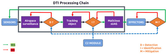
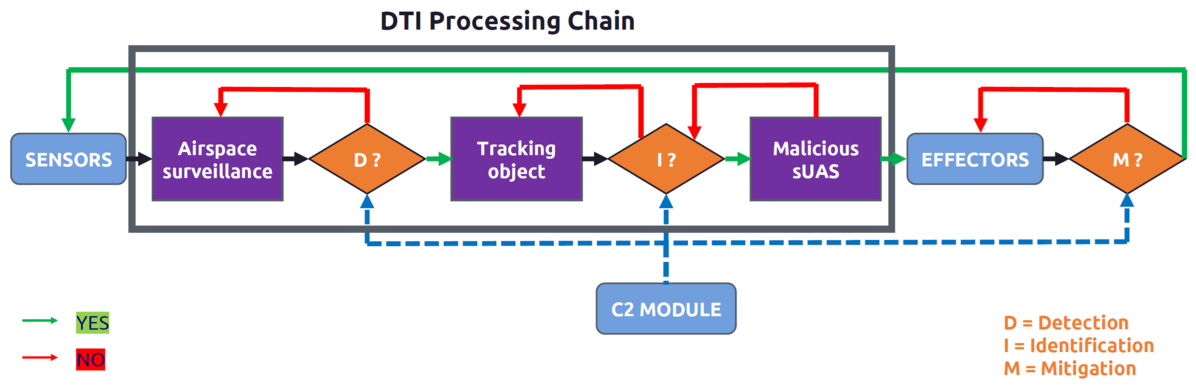
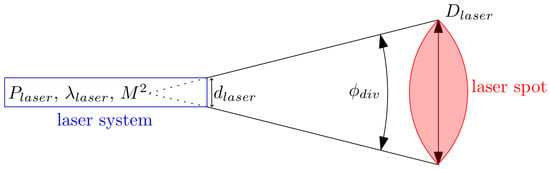
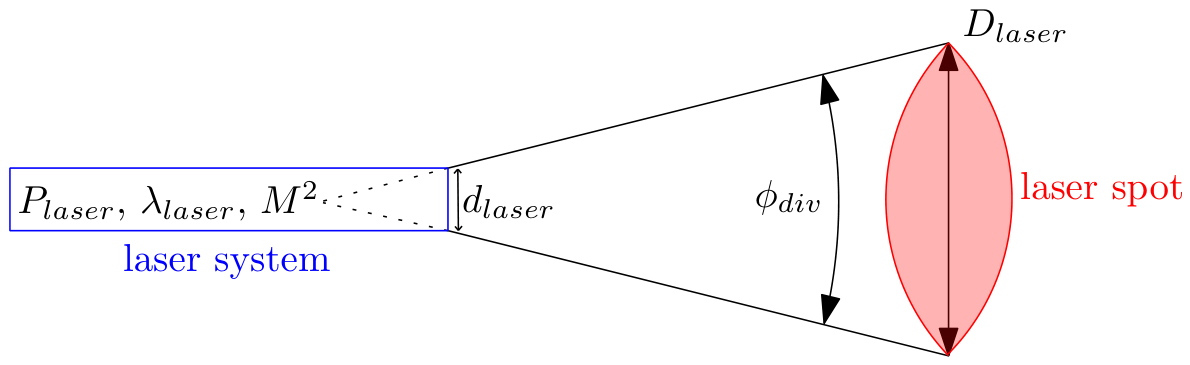
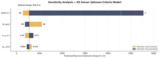
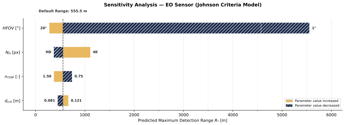
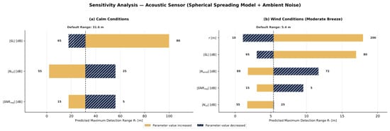
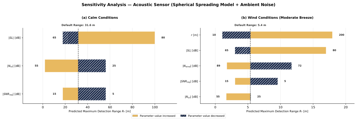
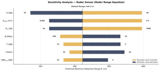
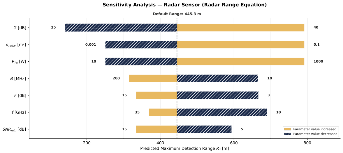

Disclaimer/Publisher’s Note: The statements, opinions and data contained in all publications are solely those of the individual author(s) and contributor(s) and not of MDPI and/or the editor(s). MDPI and/or the editor(s) disclaim responsibility for any injury to people or property resulting from any ideas, methods, instructions or products referred to in the content. |
© 2026 by the authors. Licensee MDPI, Basel, Switzerland. This article is an open access article distributed under the terms and conditions of the Creative Commons Attribution (CC BY) license.