UAV-Based Retrieval of Soil Organic Matter During the Bare-Soil Period: Effects of Surface Tillage Status

Highlights

What are the main findings?

• Surface tillage status markedly changed the relationships between SOM and UAV multispectral reflectance during the bare-soil period.
• Under the random-split held-out test set, status-specific SOM retrieval models outperformed the combined-dataset model, with the highest test-set $R^2$ values reaching 0.84 and 0.85 under the plowed-leveled and plowed-unleveled statuses, respectively.

What are the implications of the main findings?

• Surface tillage status should be considered as an important source of surface heterogeneity in UAV-based SOM retrieval.
• A retrieval method that accounts for surface tillage status can improve field-scale SOM retrieval under the present study conditions and provide a reference for pre-sowing precision management.

Abstract

Unmanned aerial vehicle (UAV) multispectral imagery provides a promising approach for field-scale retrieval of soil organic matter (SOM) during the bare-soil period. However, tillage-induced surface heterogeneity is often overlooked. This heterogeneity may alter soil spectral responses and model performance. This study examined the effects of surface tillage status on UAV-based SOM retrieval in farmland. UAV multispectral imagery and 108 topsoil samples were collected during the bare-soil period. The SOM values ranged from 1.37 to 30.95 g/kg. Analyses were conducted under three tillage-status settings: undifferentiated tillage status, plowed-leveled status, and plowed-unleveled status. Spectral and textural features were extracted and selected using a genetic algorithm. These features were then used to develop SOM retrieval models with random forest regression, extreme gradient boosting, and support vector regression. For the six original multispectral bands, the correlations between SOM and band reflectance differed among tillage-status settings. They were weak under the undifferentiated tillage status. They were significantly negative under the plowed-leveled status and significantly positive under the plowed-unleveled status. Texture-derived indicators and standard normal variate analysis suggested that the positive correlations under the plowed-unleveled status may be partly associated with surface-structure-related spectral amplitude effects. Integrating textural features improved the overall test-set accuracy metrics. However, statistically detectable reductions in absolute prediction error were mainly observed under the plowed-unleveled status. On the random-split held-out test set, the highest $R^2$ values reached 0.84 and 0.85 under the plowed-leveled and plowed-unleveled statuses, respectively. These results indicate that surface tillage status is an important source of surface heterogeneity. It should therefore be explicitly considered in UAV-based SOM retrieval under the present study conditions.

1. Introduction

Soil organic matter (SOM) is a key component of soil fertility. It is also an important determinant of crop production capacity. This is because SOM affects nutrient supply, water and nutrient retention, and aggregate stability [1]. In precision agriculture, timely and reliable mapping of SOM spatial variability is increasingly needed. This information supports site-specific management, organic amendment, and tillage optimization [2]. Conventional SOM monitoring relies on manual sampling and laboratory analysis. These methods are labor-intensive, time-consuming, and difficult to conduct at high frequency [3]. With the development of low-altitude remote sensing, unmanned aerial vehicle (UAV)-based multispectral observation has become an efficient alternative for SOM retrieval [4,5]. For field-scale monitoring, low-altitude UAV imagery is less affected by atmospheric interference. It also provides higher spatial resolution and greater operational flexibility [6,7]. Centimeter-level imagery can capture soil clods and microtopographic features on bare soil surfaces. These surface characteristics can be quantified using spectral and textural metrics [8,9]. Therefore, UAV multispectral imagery has received increasing attention for SOM retrieval during the bare-soil period [10,11,12].

Substantial progress has been made in SOM retrieval using UAV remote sensing. Existing studies can be broadly divided into two approaches. The first approach estimates SOM indirectly during the crop growth period. It uses canopy spectral information as an intermediate representation [13,14]. In this approach, crops are treated as the observation target. Vegetation indices are then extracted from UAV imagery. These indices are used to link crop growth status with SOM content. Wang et al. and Xie et al. [13,14] showed that canopy information acquired at the winter wheat jointing stage can be used to estimate topsoil SOM. This approach is not restricted by the short bare-soil observation window. It also provides more opportunities for image acquisition during the crop growth period [4,15,16]. However, canopy spectra are affected by many factors other than SOM. These factors include soil moisture, fertilization, and crop growth conditions. Such multifactor interference makes it difficult to isolate the spectral response associated with SOM. This can reduce model generalization ability [17,18,19,20]. The second approach retrieves SOM directly from exposed soil spectral information during the bare-soil period [5,21]. This approach uses the soil surface as the observation target. It derives spectral reflectance from UAV imagery and establishes quantitative relationships between soil spectral features and SOM content. Zhou et al. [5] used UAV multispectral imagery during the bare-soil period and achieved good retrieval performance with machine learning models. Previous studies have also shown that textural features can complement spectral information. They can describe soil aggregate structure, local gray-level variation, and microtopographic patterns [10,21,22]. Wang et al. [21] reported that combining texture with spectral indices improved SOM estimation accuracy. Compared with canopy-based retrieval, direct bare-soil retrieval avoids uncertainty caused by canopy occlusion and crop physiological variation. It can therefore better represent soil surface spectral responses [11,23,24]. However, the bare-soil period does not necessarily provide a homogeneous observation background. Pre-sowing tillage operations can modify soil surface structure. They can change clod size, ridge-furrow morphology, surface roughness, and the proportion of exposed soil facets. A rough plowed surface increases local illumination differences. It also increases cast shadows and self-shadowing. These effects can enhance directional scattering and produce mixed bright and shaded pixels in UAV images. In contrast, leveling and rotary tillage can break large clods and smooth the soil surface. This reduces shadow fractions and changes the reflectance distribution observed by the sensor. At the centimeter scale of UAV imagery, these microtopographic changes may introduce reflectance-amplitude disturbances. These disturbances may mask or modify the intrinsic spectral response of SOM [8,25,26,27]. Therefore, surface tillage status should be considered as an important source of bare-soil background variation in UAV-based SOM retrieval. Model performance is also affected by feature selection and modeling algorithms. Commonly used algorithms include random forest regression (RFR), extreme gradient boosting (XGBoost), and support vector regression (SVR). Heil et al. [10] achieved accurate SOM retrieval using RFR. Xia et al. [15] developed an SOM retrieval model using XGBoost and obtained reliable predictions. Yuan et al. [28] estimated SOM using SVR. These algorithms have shown good performance in previous SOM retrieval studies. However, their applicability across different surface tillage statuses remains unclear.

Based on these considerations, typical farmland areas in Changji City and Hutubi County, Xinjiang, China, were selected as the study area. UAV multispectral imagery and soil samples were collected during the bare-soil period before spring sowing. Field surveys and farming records were also used to identify surface tillage status. The specific contribution of this study is to treat tillage-induced surface heterogeneity as an important source of bare-soil background variation in UAV-based SOM retrieval. It is not treated only as a general field-management description. Analyses were conducted under three tillage-status settings: undifferentiated tillage status, plowed-leveled status, and plowed-unleveled status. Based on feature selection results, SOM retrieval models were developed using spectral and textural features. Three machine learning algorithms were compared: RFR, XGBoost, and SVR. We hypothesized that surface tillage status modifies soil surface roughness and shadow distribution. This modification changes the relationship between SOM and UAV-derived reflectance. We also hypothesized that textural features can capture part of the tillage-induced surface heterogeneity. Therefore, they may improve SOM retrieval compared with spectral features alone. Finally, we hypothesized that status-specific modeling can improve prediction accuracy and model stability compared with undifferentiated tillage modeling.

2. Materials and Methods

2.1. Study Area

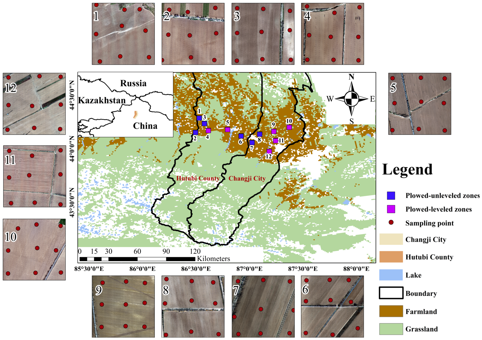
The study area is located in parts of Changji City and Hutubi County, Changji Hui Autonomous Prefecture, Xinjiang, China (86°00′–87°30′ E, 44°00′–44°30′ N; Figure 1). It lies on an alluvial plain along the northern piedmont of the Tianshan Mountains. The region has a temperate continental arid climate. It is characterized by limited rainfall and strong evaporative demand. Across the agricultural plains of Changji, mean annual precipitation is approximately 150–190 mm. Annual evaporation is about 1500–2100 mm [29,30]. In spring, the soil surface dries rapidly under arid conditions. This may reduce the influence of soil moisture on soil spectral responses [29,30,31]. Soil texture data from the 0–20 cm samples collected at the field sampling sites showed that the soils were mainly silt loam and silty clay loam. During field sampling, no obvious visible salt patches or continuous surface crusts were observed in field records or photographs. The main cultivated crops in this area are cotton and maize [32,33].

2.2. Technical Framework

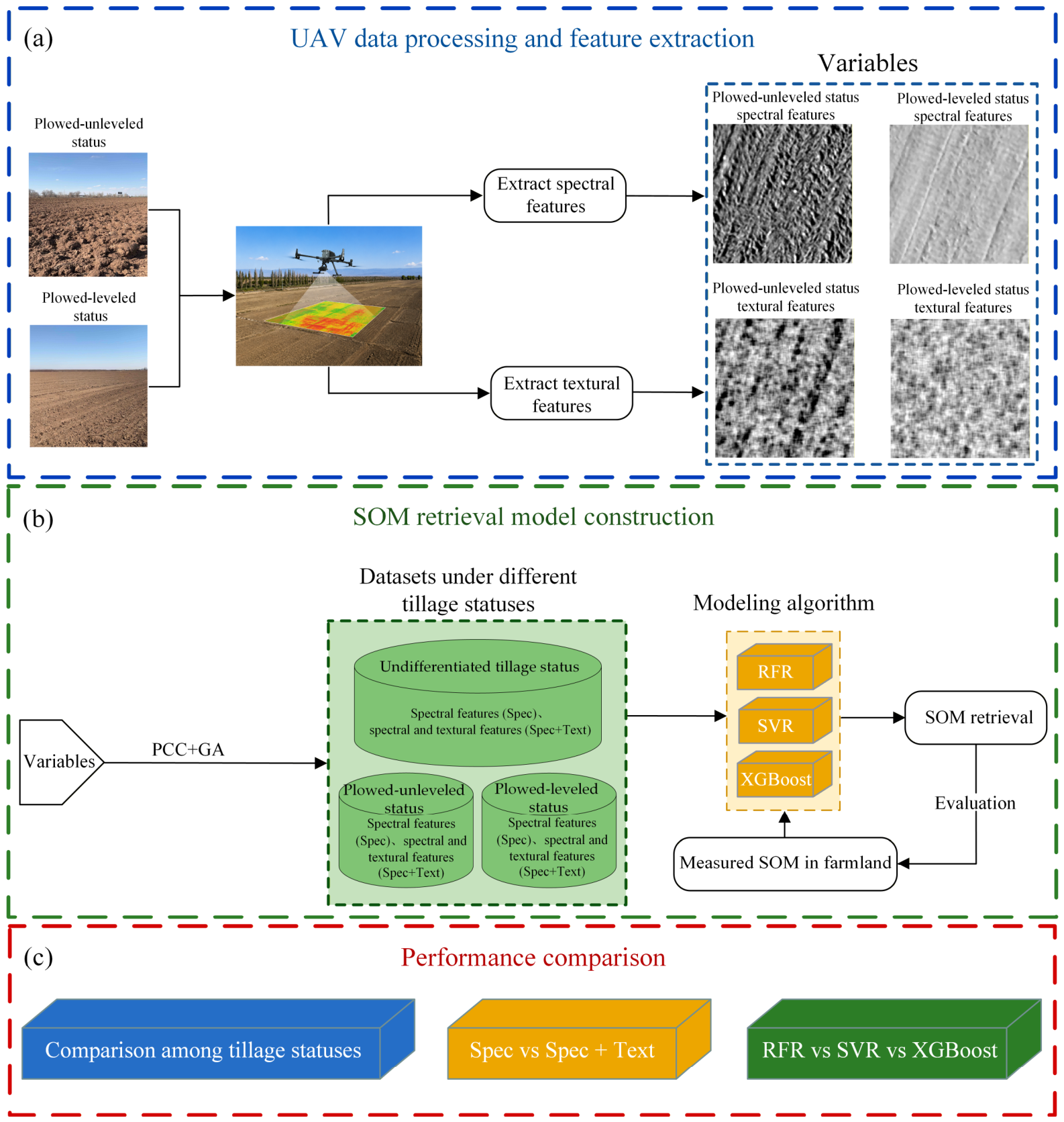
The overall technical framework of this study is shown in Figure 2. It consisted of three main components. The first component was UAV data processing and feature extraction. The second component was the SOM retrieval model construction under different surface tillage statuses. The third component was performance comparison among tillage statuses, feature combinations, and modeling algorithms.

2.3. Soil Sampling and Auxiliary Data Collection

2.3.1. SOM Data Collection

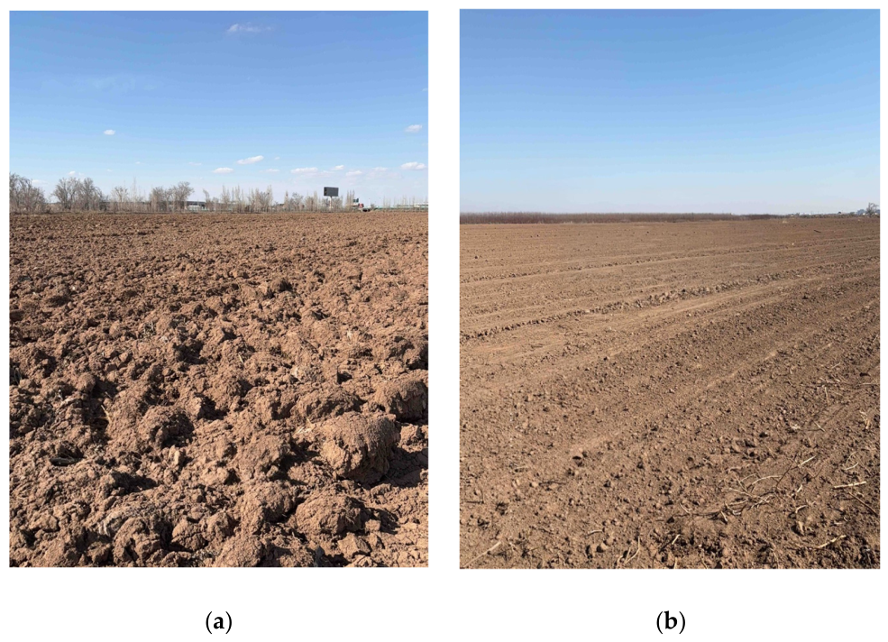
Soil sampling was conducted in early April 2024. At this time, the study area was undergoing pre-sowing field preparation. Farmland surfaces were largely free of crop residues and other cover. This provided favorable conditions for soil spectral acquisition during the bare-soil period (Figure 3). To ensure spatial representativeness and capture different surface tillage statuses, 12 sampling zones were established. Each zone measured 500 m × 500 m. Nine sampling points were uniformly distributed within each zone. This resulted in a total of 108 soil samples (Figure 1). Based on field surveys, farming records, and surface characteristics, the zones were classified into two categories. Six zones were identified as the plowed-unleveled status. These areas had been plowed but not harrowed. They were characterized by large soil clods and ridge-furrow structures (Figure 3a). The remaining six zones were classified as the plowed-leveled status. In these areas, the soil surface had been rotary-tilled and mechanically leveled after plowing. This formed a relatively smooth surface with finer soil particles (Figure 3b). Based on this classification, analyses were conducted under three tillage-status settings. These were the undifferentiated tillage status, the plowed-leveled status, and the plowed-unleveled status. The undifferentiated tillage status represented a combined dataset in which all samples were analyzed together. The plowed-leveled and plowed-unleveled statuses represented datasets that included only samples from the corresponding surface condition.

Figure 2. Workflow of the proposed method. (a) UAV data processing and feature extraction; (b) SOM retrieval model construction; (c) Performance comparison.

Figure 2. Workflow of the proposed method. (a) UAV data processing and feature extraction; (b) SOM retrieval model construction; (c) Performance comparison.

At each sampling point, surface soil was collected from a depth of 0–20 cm using the five-point composite sampling method. This depth was selected because it corresponds to the main cultivated plow layer in the study area. Previous studies have shown that plowing can promote relatively uniform SOC or nutrient distributions within the plow layer [34,35]. Handheld GPS (GPSMAP 64sx, Garmin International Inc., Olathe, KS, USA) coordinates and field photographs were recorded at each sampling point. These records were used to support image registration and verification of tillage status. To reduce positional mismatch between field sampling points and UAV imagery, a white marker board was placed 1.5 m north of each soil sampling point. The board appeared as a bright marker in the UAV orthomosaic. The final sampling position was then determined as the location 1.5 m south of this marker, with support from* handheld GPS coordinates. After air-drying and sieving through a 100-mesh sieve, SOM content was determined using the potassium dichromate volumetric method [36].

Table 1. Zone-level SOM statistics and tillage-status classification of sampling zones.

Zone ID	Sampling Date	Tillage Status	Samples	Mean g/kg	Standard Deviation	Maximum	Minimum	Coefficient of Variation (%)
1	8 April 2024	Plowed-unleveled	9	23.81	3.24	30.95	20.86	13.60
2	11 April 2024	Plowed-unleveled	9	3.34	1.70	6.64	1.37	50.96
3	8 April 2024	Plowed-unleveled	9	17.93	4.39	25.89	12.83	24.50
4	11 April 2024	Plowed-leveled	9	14.11	1.60	16.27	11.46	11.38
5	10 April 2024	Plowed-leveled	9	27.68	1.65	30.24	24.75	5.96
6	6 April 2024	Plowed-unleveled	9	15.94	1.75	18.34	13.06	11.00
7	6 April 2024	Plowed-unleveled	9	15.91	2.85	21.77	13.51	17.88
8	9 April 2024	Plowed-unleveled	9	16.65	3.32	22.45	12.83	19.97
9	7 April 2024	Plowed-leveled	9	26.91	2.75	30.93	22.00	10.21
10	7 April 2024	Plowed-leveled	9	12.84	6.94	21.55	1.60	54.07
11	11 April 2024	Plowed-leveled	9	19.78	1.79	22.92	16.73	9.06
12	5 April 2024	Plowed-leveled	9	14.52	1.68	16.73	12.15	11.55

shows the basic statistics of the SOM samples.

2.3.2. Auxiliary Environmental Data Collection

To evaluate whether the two tillage-status groups differed in basic soil and environmental background conditions, auxiliary variables were compiled at the sampling-zone level. Soil particle-size composition was measured using a BT-9300S automatic laser particle-size analyzer (Dandong Bettersize Instruments Ltd., Dandong, China). The proportions of clay, silt, and sand were then calculated. Soil texture classes were assigned accordingly. Surface soil moisture was not measured synchronously during UAV image acquisition and soil sampling. Therefore, volumetric soil water content from ERA5-Land was used as a near-surface soil moisture proxy [37]. The corresponding values were extracted for each sampling zone according to the sampling date and zone location. These ERA5-Land data were used only as auxiliary background information. They were not included as model input variables. Because ERA5-Land has a coarser spatial resolution than the 500 m × 500 m sampling zones, this variable should be interpreted as a regional moisture-background proxy. It should not be regarded as direct field-measured soil moisture.

The zone-level soil texture, soil moisture proxy, and tillage-status information are provided in

Table A1. Zone-level soil texture and moisture characteristics of the 12 sampling zones.

Zone ID	Sampling Date	Tillage Status	Volumetric Soil Water Content Proxy (m3/m3)	Clay (%)	Silt (%)	Sand (%)	Soil Texture
1	8 April 2024	Plowed-unleveled	0.08	31.27	56.71	12.01	Silty clay loam
2	11 April 2024	Plowed-unleveled	0.17	19.36	52.42	28.22	Silt loam
3	8 April 2024	Plowed-unleveled	0.08	21.70	51.95	26.35	Silt loam
4	11 April 2024	Plowed-leveled	0.09	13.36	59.01	27.63	Silt loam
5	10 April 2024	Plowed-leveled	0.18	18.22	47.07	34.71	Silty clay loam
6	6 April 2024	Plowed-unleveled	0.20	11.88	51.63	36.49	Silt loam
7	6 April 2024	Plowed-unleveled	0.09	14.26	53.73	32.00	Silt loam
8	9 April 2024	Plowed-unleveled	0.05	11.61	46.89	41.50	Loam
9	7 April 2024	Plowed-leveled	0.17	13.45	52.56	33.99	Silt loam
10	7 April 2024	Plowed-leveled	0.05	17.28	43.28	39.44	Loam
11	11 April 2024	Plowed-leveled	0.11	24.74	55.45	19.81	Silt loam
12	5 April 2024	Plowed-leveled	0.26	11.95	51.54	36.51	Silt loam

. Detailed plot-level information on irrigation, fertilization, salinity, and crop-rotation history was not systematically surveyed or completely recorded for all sampling zones. Therefore, the background comparison focused on the available zone-level variables. These variables included SOM, soil texture, and the soil moisture proxy.

2.4. UAV Data Acquisition and Preprocessing

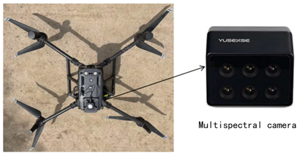
UAV imagery was acquired using a DJI M300 RTK platform (Matrice 300 Real-Time Kinematic, DJI Innovation Technology Co., Ltd., Shenzhen, China) equipped with an MS600 Pro multispectral camera (YUSENSE (Changguang Yuchen) Co., Ltd., Qingdao, China), as shown in Figure 4. The camera has a resolution of 1.2 megapixels and records six spectral bands, including blue, green, red, nir, rededge1, and rededge2. UAV image acquisition was performed between 12:00 and 15:00 under clear, windless, and stable illumination conditions. Radiometric calibration was conducted before each UAV takeoff using the calibrated gray reference panel supplied with the MS600 Pro multispectral camera. The band information and band-specific panel reflectance values are listed in

Table 2. Band information and panel reflectance.

Band	Spatial Resolution (m)	Center Wavelength (nm)	Reflectance of Calibration Panel
B1—Blue	0.07	450	0.65
B2—Green	0.07	555	0.63
B3—Red	0.07	660	0.62
B4—RedEdge1	0.07	720	0.61
B5—RedEdge2	0.07	750	0.60
B6—NIR	0.07	840	0.59

. During calibration, the camera lens was aligned with the center of the gray panel, and an image of the panel was acquired before each flight mission. The flight altitude was 100 m, and both forward and side overlaps were set to 80%. After image acquisition, radiometric correction was conducted using Yusense Ref software (version 3.2, YUSENSE (Changguang Yuchen) Co., Ltd., Qingdao, China). The multispectral images were then mosaicked in Pix4D Mapper software (version 4.5.6, Pix4D S.A., Prilly, Switzerland). For each flight, six single-band reflectance images were produced. The 16-bit scaled reflectance images were subsequently converted to unitless reflectance values ranging from 0 to 1 in ENVI software (version 5.6, L3Harris Geospatial, Boulder, CO, USA) by dividing the pixel values by 65,535. ArcGIS software (version 10.7, Esri Inc., Redlands, CA, USA) was used to delineate plot boundaries and generate shapefiles.

2.5. Image Feature Extraction

2.5.1. Texture Feature Construction

In this study, a multidimensional set of textural features was constructed in Python software (version 3.10, Python Software Foundation, Wilmington, DE, USA). This feature set included first-order statistics, second-order statistics, and spatial gradient information. Second-order statistical features were derived from the gray-level co-occurrence matrix (GLCM). A 15 × 15-pixel moving window was used with a step size of 3 pixels. The window size was selected by considering the UAV image spatial resolution and the surface structures targeted by the texture analysis. At a UAV image resolution of 0.07 m, this window corresponded to approximately 1.05 m × 1.05 m on the ground. This ground coverage was considered suitable for capturing local gray-level patterns associated with field-observed soil clods, ridge-furrow microtopography, and edge information. It also avoided excessive smoothing of local surface heterogeneity. This choice is consistent with the general principle of GLCM texture analysis. The moving window should be large enough to represent the texture elements of interest. It should not be so large that it mixes different surface patterns [38]. Mean values were calculated across four directions: 0°, 45°, 90°, and 135°. Eight GLCM parameters were obtained. These included MEA, VAR, HOM, CON, DIS, ENT, ASM, and COR. Additional features were constructed to describe local gray-level fluctuation and high-frequency edge information. Local standard deviation (STD) was calculated from first-order statistics. Laplacian energy (LAPEN) was derived using spatial filtering. Both features were computed using the same window settings [39,40]. In total, 60 textural indicators were constructed.

Among these textural features, STD, VAR, ENT, and HOM were used as texture-derived proxies for surface heterogeneity. STD and VAR describe local gray-level fluctuation and dispersion. ENT represents texture complexity. HOM represents local uniformity. These metrics were first calculated separately for each multispectral band. They were then averaged across the six bands to obtain Mean_STD, Mean_VAR, Mean_ENT, and Mean_HOM. These band-averaged metrics provided compact descriptors of overall surface texture.

2.5.2. Spectral Feature Construction

Compared with single-band reflectance, band-combination spectral features can provide additional surface information. They can also reduce the influence of imaging conditions on reflectance to some extent [41]. In this study, 103 spectral features were constructed. The calculation formulas for all spectral indices are presented in

Table 3. Spectral index formulas.

Number	Spectral Indices	Formula	Reference
1–6	Band Reflectance (Bi)	$b_i$	-
7–11	NLI-form nonlinear band-combination index (NLIi)	$(b_{\mathrm{i}}^2-b_3)/(b_{\mathrm{i}}^2+b_3)$	[42]
12–26	Brightness Index (BIij)	$(b_i^2+b_j^2{)}^{0.5}$	[43]
27–46	Brightness Index 2 (BIijk)	$(b_i^2+b_j^2+b_k^2{)}^{0.5}/3$	[44]
47–52	Natural Logarithm of Band Reflectance (ln(Bi))	$\mathrm{L}\mathrm{n}(b_i)$	[45]
53–67	Difference Index (Dij)	$b_i-b_j$	[46]
68–97	Ratio Index (Rij)	$b_i/b_{j^{\prime }}$	[47]
98–103	Reciprocal of Band Reflectance (REi)	$1/b_i$	[48]

.

2.5.3. Sample-Level Extraction of Spectral and Textural Values

To link UAV-derived image features with laboratory-measured SOM values, sample-level spectral and textural values were extracted according to the GPS coordinates of the soil sampling points. The sampling point shapefiles were overlaid on the UAV-derived spectral and textural feature rasters. The same coordinate system was used for all layers. Each sampling point was then matched with its corresponding raster location. For spectral features, a 3 × 3-pixel window centered on each sampling point was used for value extraction. The median value within this window was calculated. This value was assigned to the corresponding soil sample as the sample-level spectral feature value. This strategy was used to reduce the influence of single-pixel noise, minor positioning errors, and local abnormal pixels. For textural features, texture layers were first generated using the moving-window approach described above. Each texture raster cell had already incorporated neighborhood information from the 15 × 15-pixel moving window. Therefore, no additional buffer was applied during point-level extraction. Instead, the texture value of the raster cell corresponding to each sampling point was directly extracted. This value was then assigned to the corresponding soil sample. The extracted spectral and textural values were finally linked to the laboratory-measured SOM data using the sample ID. These linked data were used for subsequent correlation analysis, feature selection, and SOM retrieval modeling.

2.6. Supporting Analysis of Surface-Structure-Related Spectral Effects

To examine the anomalous positive association between SOM and soil reflectance under the plowed-unleveled status, the standard normal variate (SNV) transformation was applied to the spectral dataset. SNV normalizes each sample spectrum, reducing baseline shifts and amplitude variations caused by particle-size differences and surface scattering [49]. The SNV transformation was calculated as follows:

$$\overline{r}={\displaystyle \frac{1}{n}}{\sum }_{i=1}^n{r}_i$$

(1)

$$\mathrm{S}\mathrm{D}=\sqrt{{\displaystyle \frac{1}{n-1}}{\sum }_{i=1}^n{\left(r_i-\overline{r}\right)}^2}$$

(2)

$$r_{\mathrm{S}\mathrm{N}\mathrm{V}}={\displaystyle \frac{r_i-\overline{r}}{\mathrm{S}\mathrm{D}}}$$

(3)

In the formula, $r_{\mathrm{S}\mathrm{N}\mathrm{V}}$ is the spectral reflectance after SNV transformation; $r_i$ is the original spectral reflectance; $\overline{r}$ and SD are the mean and standard deviation of spectral reflectance across all bands for the sample, respectively; and $n$ is the number of bands, with $n=6$ in this study.

The supporting logic is as follows. If the positive correlation is mainly driven by surface roughness and scattering effects, it should weaken or reverse after an SNV transformation. If the correlation remains stable, it is more likely to reflect intrinsic spectral properties of the soil.

2.7. Feature Selection

The number of input features and feature redundancy can strongly affect model accuracy and generalization ability [50]. To improve feature effectiveness and reduce redundant information, a two-stage feature selection strategy was applied under all three surface tillage statuses. The first stage was preliminary feature screening. This step was performed using only the training set. Pearson correlation coefficients (|R|) between SOM and each spectral or textural feature were calculated separately [51]. Based on the magnitude of |R|, the top 40 spectral features and the top 20 textural features were retained. These features formed the spectral and textural candidate pools, respectively. The second stage was feature subset optimization using a genetic algorithm (GA). The candidate features from the first stage were used as inputs. Optimization was conducted separately for spectral and textural features. A GA-based search strategy was used to identify the optimal feature subsets. The fitness function was defined as the five-fold cross-validation performance of random forest regression (RFR) [52]. The resulting subsets were used as inputs for subsequent SOM retrieval modeling. The detailed GA parameter settings are provided in

Table A2. Parameter settings of GA-based feature subset optimization.

Parameter	Setting
Candidate feature pool	Spectral features: 40; textural features: 20
Optimization strategy	Spectral and textural features optimized separately
Candidate subset size for spectral features	2–10
Candidate subset size for textural features	2–5
Random seed	45
Wrapper estimator	Random forest regression (RFR)
Fitness evaluation	5-fold CV (training set)
Population size	20
Maximum number of generations	30
Crossover rate	1.0
Mutation rate	0.05–0.30
Early-stopping criterion	7
Minimum improvement threshold	0.001
Redundancy penalty	Maximum absolute correlation among selected features
Redundancy penalty weight	0.2
Fitness function	$R^{2}CV-0.20\times \mathit{redundancy} \mathit{penalty}-0.05\times \mathit{rRMSECV}$

Note: $R^2$ CV and rRMSECV represent the mean $R^2$ and rRMSE obtained from five-fold cross-validation on the training set, respectively.

.

For the final feature subsets reported in this study, the GA random seed was fixed at 45 to ensure reproducibility. GA-based feature selection is a stochastic optimization procedure. Therefore, the selected feature subsets may vary with random population initialization, crossover, and mutation. To evaluate feature-selection stability, the GA procedure was repeated 50 times using random seeds from 1 to 50. The GA parameter settings were kept unchanged. The selection frequency of each feature was calculated as the proportion of repetitions in which that feature was selected. The use of 50 repetitions provided a practical balance between computational cost and stability-assessment resolution. It allowed selection frequencies to be summarized at 2% intervals.

2.8. Model Construction

RFR, XGBoost, and SVR were used to construct SOM retrieval models [53,54,55]. Before model training, stratified random sampling was used to divide the dataset. This procedure was used to ensure comparable SOM distributions between the training and test sets. With reference to the SOM classification standard from the Second National Soil Survey of China and the sample distribution of this study, SOM content was divided into four classes. These classes were Very Low (<10 g/kg), Low (10–20 g/kg), Medium (20–30 g/kg), and High (≥30 g/kg) [56]. Stratification was performed based on these four classes. Within each class, samples were randomly split into training and test sets at a 7:3 ratio. Model training and validation were conducted in Python 3.10. Because the three algorithms differ in their sensitivity to feature scaling, z-score normalization was applied before SVR modeling. The normalization parameters were calculated from the training set. The same parameters were then applied to the test set. No standardization was applied for RFR or XGBoost. For all three models, hyperparameters were optimized on the training set using random search combined with five-fold cross-validation [57,58]. After the optimal hyperparameters were identified, each model was refitted using all training samples. The refitted models were then evaluated on the held-out test set. The detailed hyperparameter search spaces are provided in

Table A3. Hyperparameter search space for RFR, XGBoost, and SVR.

Model	Hyperparameter	Search Range
RFR	n_estimators	400–2000
	max_depth	4–20
	min_samples_split	2–20
	min_samples_leaf	1–10
	max_features	sqrt, log2, None, 0.5, 0.7
	max_samples	0.6–1.0
XGBoost	n_estimators	800–3000
	max_depth	3–8
	learning_rate	0.02–0.10
	min_child_weight	1–20
	subsample	0.5–1.0
	colsample_bytree	0.5–1.0
	gamma	0–5
	reg_alpha	0–10
	reg_lambda	1–51
SVR	C	0.01, 0.1, 0.5, 1, 2, 5, 10, 20
	epsilon	0.001, 0.01, 0.05, 0.1, 0.2, 0.5
	gamma	scale, auto, 0.001, 0.01, 0.1, 1.0

.

2.9. Model Accuracy Evaluation

Model performance was evaluated using $R^2$, rRMSE, LCCC, and RPD to provide a comprehensive assessment of predictive accuracy. The formulas are given as follows:

$$R^2=1-{\displaystyle \frac{{\displaystyle {\sum }_{i=1}^n}(y_i-{\widehat{y}}_i{)}^2}{{\displaystyle {\sum }_{i=1}^n}(y_i-\overline{y}{)}^2}}$$

(4)

$$\mathrm{r}\mathrm{R}\mathrm{M}\mathrm{S}\mathrm{E}={\displaystyle \frac{\sqrt{\frac{1}{n}{\sum }_{i=1}^n{\left(y_i-{\widehat{y}}_i\right)}^2}}{\overline{y}}}$$

(5)

$$\mathrm{L}\mathrm{C}\mathrm{C}\mathrm{C}={\displaystyle \frac{2R{s}_y{s}_{\widehat{y}}}{s_y^2+s_{\widehat{y}}^2+{\left(\overline{y}-\overline{\widehat{y}}\right)}^2}}$$

(6)

$$\mathrm{R}\mathrm{P}\mathrm{D}={\displaystyle \frac{s_y}{\sqrt{\frac{1}{n}{\sum }_{i=1}^n{\left(y_i-{\widehat{y}}_i\right)}^2}}}$$

(7)

where $y_i$ and ${\widehat{y}}_i$ are the measured and predicted SOM values of the $i$-th sample, respectively, and $n$ is the total number of samples. The terms $\overline{y}$ and $\overline{\widehat{y}}$ are the mean values of the measured and predicted data, respectively. The terms $s_y$ and $s_{\widehat{\mathrm{y}}}$ are the corresponding standard deviations. The term $R$ is the Pearson correlation coefficient between measured and predicted values.

The $R^2$ value reflects the proportion of variance in the measured data explained by the model. Its value ranges from 0 to 1, with values closer to 1 indicating better model fit and stronger explanatory power [59]. The rRMSE represents prediction error relative to the mean of the measured values. A smaller rRMSE indicates higher predictive accuracy and lower error [60]. The RPD was used to assess predictive ability. An RPD value below 1.5 indicates weak predictive ability. A value between 1.5 and 2.0 indicates good predictive ability. A value above 2.0 indicates excellent predictive accuracy [61]. The LCCC was used to evaluate the agreement between predicted and measured values. An LCCC value above 0.90 indicates almost perfect agreement. A value of 0.80–0.90 indicates strong agreement. A value of 0.65–0.80 indicates moderate agreement. A value of 0.65 or below indicates weak agreement [62,63].

To compare model stability during training, five-fold cross-validation was performed on the training set. The mean and standard deviation of $R^2$ and rRMSE were calculated across the five folds. The mean value reflected the average model performance. The standard deviation reflected variation across different data partitions. A smaller standard deviation indicated better model stability. The cross-validation results were mainly used to assess model stability. They were interpreted together with the held-out test-set results to evaluate overall model performance. In addition to the random-split test-set evaluation, leave-one-zone-out (LOZO) validation was conducted as a supplementary spatially separated robustness assessment. This analysis was performed for the optimal spectral-plus-texture model under each tillage-status setting. It followed the general rationale of spatially separated cross-validation [64]. In each iteration, one sampling zone was left out for validation. The remaining zones were used for model training. Model performance was summarized using pooled predictions from all left-out zones and fold-wise mean ± SD values.

2.10. Statistical Analysis

Statistical tests were used to assess sample balance, background differences, and model-performance differences. Differences in SOM content between the training and test sets were tested using two-sided Mann–Whitney U tests. The same test was used to compare background variables between the plowed-leveled and plowed-unleveled groups. These variables included SOM content, soil moisture proxy, clay content, silt content, and sand content. Changes in sample-level absolute prediction errors between the spectral-only and spectral-plus-texture models were assessed using two-sided paired Wilcoxon signed-rank tests. Pairwise error differences among RFR, XGBoost, and SVR under the spectral-plus-texture setting were also assessed using two-sided paired Wilcoxon signed-rank tests. Statistical significance was denoted as follows: * p < 0.05, ** p < 0.01, *** p < 0.001, and ns, p ≥ 0.05. For the SNV-based supporting analysis, the significance of SNV-induced changes in correlation coefficients was assessed using paired bootstrap resampling.

3. Results

3.1. SOM Distribution and Background Comparison

3.1.1. SOM Distribution and Training–Test Set Balance

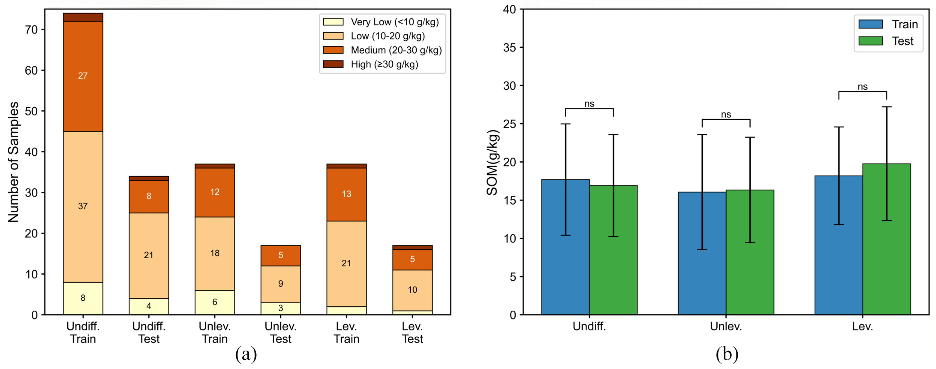
Using the SOM classes defined in Section 2.8, Figure 5a shows the distribution of sample counts across SOM classes. Results are presented for the training and test sets under the undifferentiated, plowed-unleveled, and plowed-leveled statuses. Overall, most samples were concentrated in the Low and Medium classes. Relatively few samples were in the Very Low and High classes. This indicates that SOM content in the sampled farmland soils was generally low to moderate during the bare-soil period. Figure 5b shows the mean SOM content ± standard deviation (Mean ± SD) for the training and test sets under the three tillage-status settings. The mean SOM values across all datasets ranged from 16.06 to 19.77 g/kg. This range further indicates an overall low-to-medium SOM level. It is also consistent with Figure 5a, where most samples were concentrated in the Low and Medium classes. Differences in mean SOM values between the training and test sets were generally small. Their dispersion levels were also similar. These results indicate good consistency between the two subsets in terms of central tendency and variability. Although the mean SOM value of the test set was slightly higher than that of the training set under some tillage-status settings, the differences were not statistically significant according to the Mann–Whitney U test (p ≥ 0.05). This suggests that the training and test sets remained well balanced after stratified sampling.

3.1.2. Soil Background Comparison Between Tillage-Status Groups

Several soil background factors may influence bare-soil reflectance and SOM retrieval accuracy. These factors include SOM content, soil moisture, and particle-size composition [65,66]. Therefore, SOM content, the soil moisture proxy, clay content, silt content, and sand content were compared between the plowed-leveled and plowed-unleveled groups. As shown in

Table 4. Comparison of soil background variables between tillage-status groups.

Variable	Plowed-Unleveled	Plowed-Leveled	p-Value	Significance
SOM (g/kg)	15.60 ± 6.70	19.31 ± 6.63	0.82	ns
Volumetric soil water content proxy (m3/m3)	0.11 ± 0.06	0.14 ± 0.08	0.42	ns
Clay (%)	18.35 ± 7.53	16.50 ± 4.72	0.94	ns
Silt (%)	52.22 ± 3.20	51.49 ± 5.66	0.94	ns
Sand (%)	29.43 ± 10.16	32.02 ± 7.14	0.70	ns

Note: Values are presented as zone-level mean ± SD. Each tillage-status group included six sampling zones. p-values were calculated using a two-sided Mann–Whitney U test. ns indicates no significant difference at p ≥ 0.05.

, the mean SOM content was 15.60 ± 6.70 g/kg in the plowed-unleveled group. It was 19.31 ± 6.63 g/kg in the plowed-leveled group. The plowed-leveled group showed a slightly higher mean SOM value. However, this difference was not statistically significant according to the Mann–Whitney U test (p = 0.82). Similarly, no statistically significant differences were observed between the two tillage-status groups for the volumetric soil water content proxy, clay content, silt content, or sand content (p ≥ 0.05). These results suggest that the two tillage-status groups were generally comparable in terms of the available soil and moisture-background variables.

3.2. Pearson Correlation Analysis of SOM and Remote Sensing Features

3.2.1. Correlation Between SOM and Spectral Reflectance

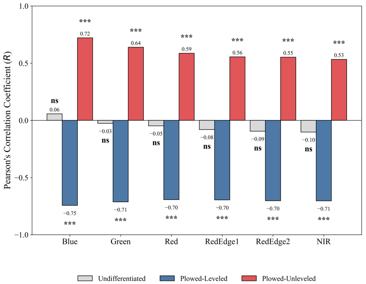
Figure 6 shows the Pearson correlation coefficients between SOM and spectral reflectance for each band. Results are presented under the undifferentiated, plowed-unleveled, and plowed-leveled statuses. Under the undifferentiated tillage status, the correlations between SOM and band reflectance were generally weak. This may be related to the mixed influence of different surface roughness conditions. Under the plowed-leveled status, SOM was significantly negatively correlated with reflectance in all bands. The R values ranged from approximately −0.75 to −0.70 (p < 0.001). This indicates a consistent negative SOM–reflectance relationship under the relatively smooth surface condition. In contrast, under the plowed-unleveled status, SOM was significantly positively correlated with reflectance across all bands. The R values ranged from approximately 0.53 to 0.72 (p < 0.001). This pattern was opposite to that observed under the plowed-leveled status.

3.2.2. Correlation of SOM with Spectral and Textural Features

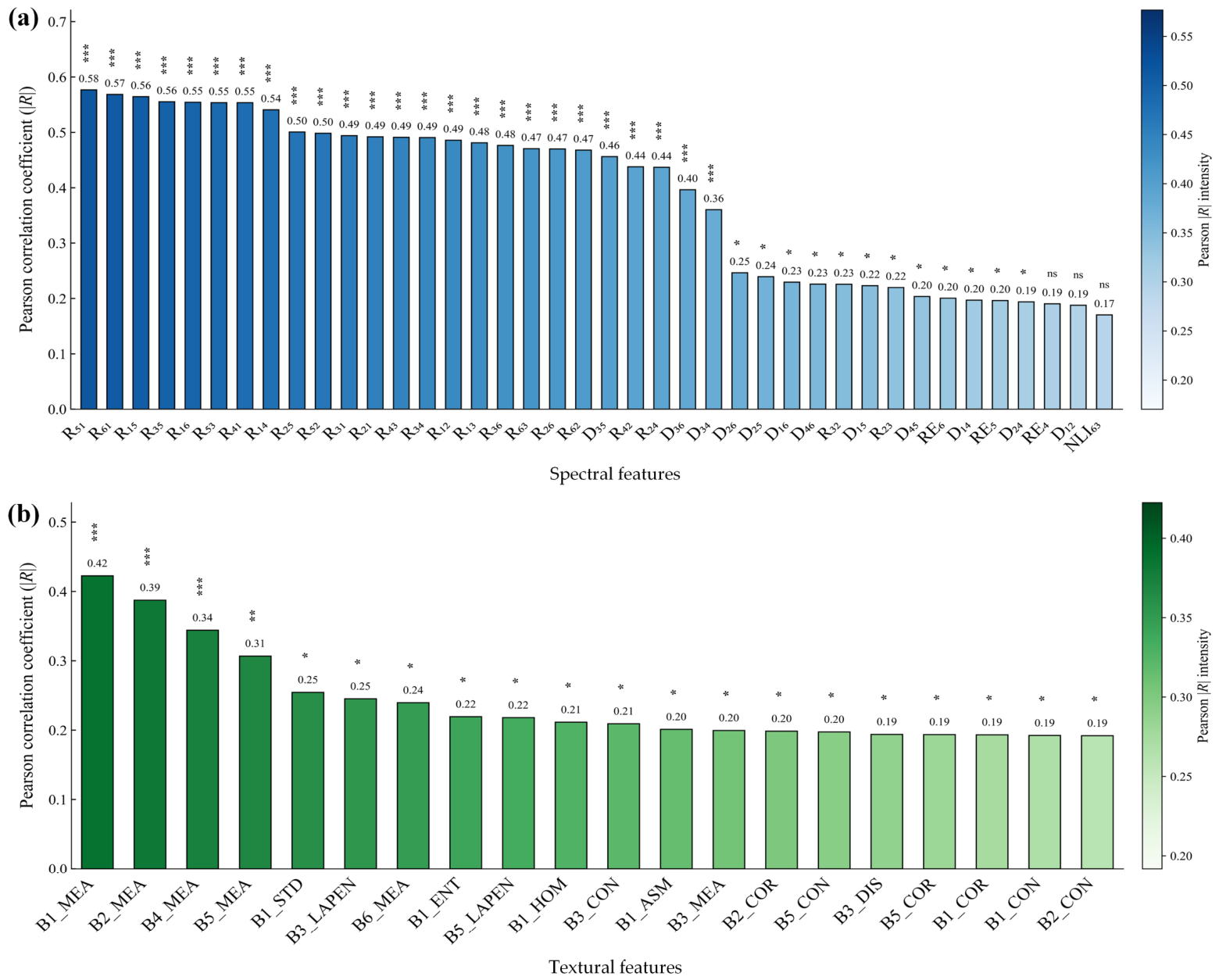
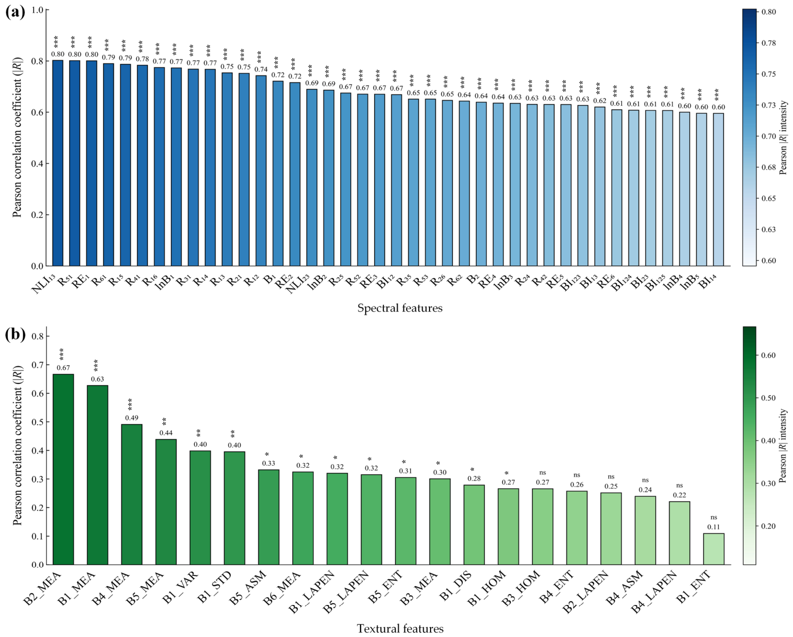
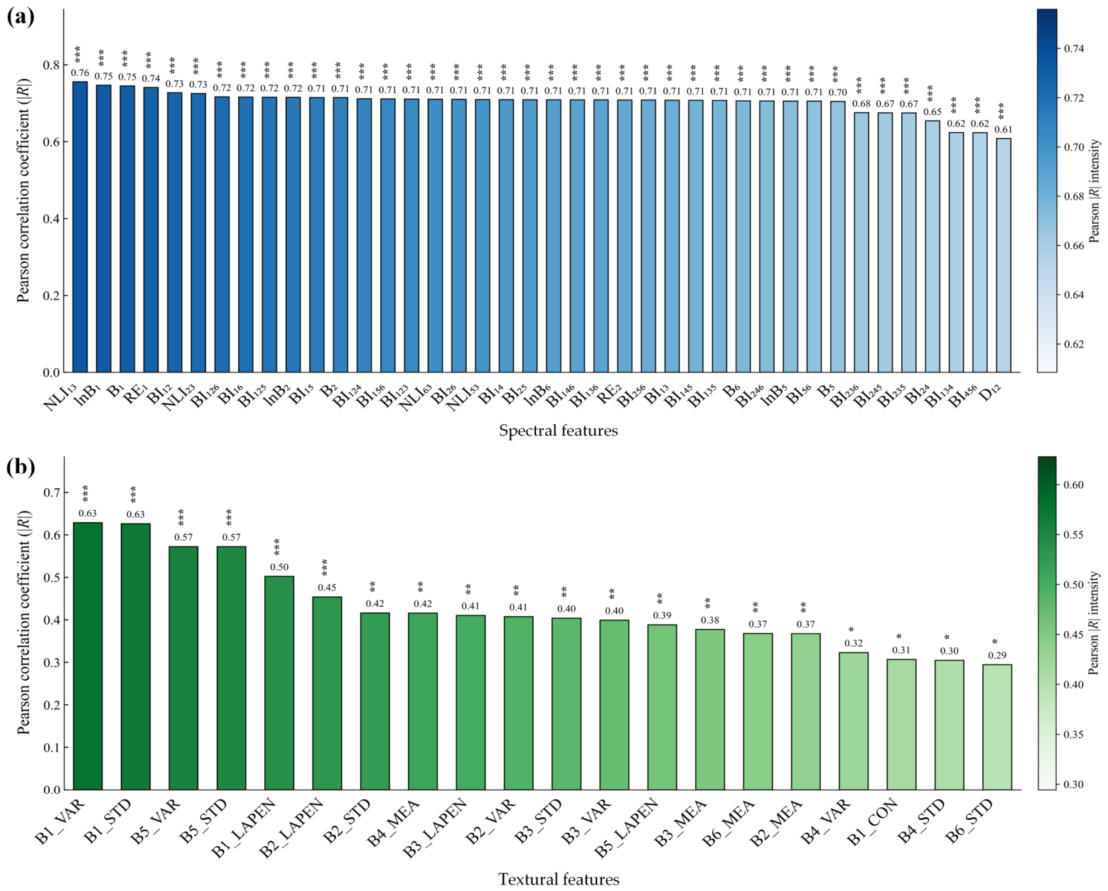
Figure 7, Figure 8 and Figure 9 show the ranked absolute Pearson correlation coefficients between SOM and spectral and textural features. Results are presented under the undifferentiated, plowed-unleveled, and plowed-leveled statuses, respectively. In each case, the top 40 spectral features and the top 20 textural features are shown.

Under the undifferentiated tillage status (Figure 7), only a few spectral features showed |R| > 0.5. All of these features were ratio indices. Among them, R₅₁ and R₆₁ showed the strongest correlations. Their |R| values were 0.58 and 0.57, respectively, and both were highly significant (p < 0.001). Among the textural features, only a few features showed |R| > 0.3. These features were mainly mean-based features. B1_MEA showed the strongest correlation, with an |R| value of 0.42 (p < 0.001).

Under the plowed-unleveled status (Figure 8), all top-ranked spectral features showed |R| > 0.6. Among them, NLI₁₃, R₅₁, and RE₁ showed the highest absolute correlations. All three features reached |R| = 0.80 (p < 0.001). Among the textural features, only two mean-based features showed |R| > 0.6. B2_MEA showed the strongest correlation, with an |R| value of 0.67 (p < 0.001).

Under the plowed-leveled status (Figure 9), all spectral features showed |R| > 0.6. Among them, NLI₁₃ showed the strongest correlation, with an |R| value of 0.76 (p < 0.001). Among the textural features, relatively few showed |R| > 0.6. Among them, B1_VAR and B1_STD showed the strongest correlations, and both had |R| values of 0.63 (p < 0.001).

3.3. Texture-Derived Surface Heterogeneity and SNV-Based Supporting Analysis

Texture-derived indicators were compared to assess image-based surface heterogeneity between the two tillage-status groups. As shown in

Table 5. Comparison of texture-derived surface heterogeneity indicators between tillage-status groups. Note: Values are presented as zone-level mean ± standard deviation. p-values were calculated using the two-sided Mann–Whitney U test. ** and *** indicate significance at the 0.01 and 0.001 levels, respectively.

Texture-Derived Indicator	Plowed-Unleveled	Plowed-Leveled	p-Value	Significance
Mean_STD	21.05 ± 1.44	20.32 ± 1.06	0.006	**
Mean_VAR	450.90 ± 59.31	417.75 ± 42.69	0.002	**
Mean_ENT	7.35 ± 0.02	6.83 ± 0.02	<0.001	***
Mean_HOM	0.085 ± 0.006	0.130 ± 0.013	<0.001	***

, the plowed-unleveled group had significantly higher Mean_STD, Mean_VAR, and Mean_ENT values than the plowed-leveled group. In contrast, Mean_HOM was significantly lower in the plowed-unleveled group. These results indicate stronger local gray-level fluctuation, greater gray-level dispersion, higher texture complexity, and lower textural homogeneity under the plowed-unleveled status.

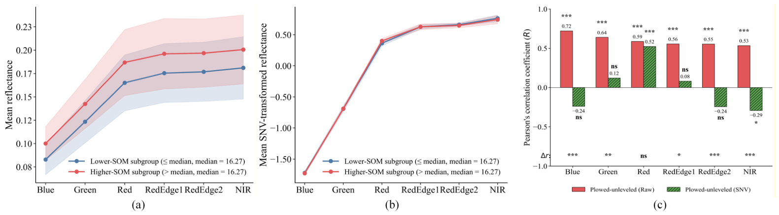
SNV transformation was further applied to the plowed-unleveled dataset as a supporting analysis. Before SNV transformation, the higher-SOM subgroup showed higher mean reflectance than the lower-SOM subgroup across all bands (Figure 10a). After SNV transformation, the spectral offset between the two subgroups was reduced (Figure 10b). The correlation analysis showed clear band-dependent changes (Figure 10c). The correlations for the Blue, RedEdge2, and NIR bands changed from positive to negative after SNV transformation. The correlations for the Green and RedEdge1 bands were weakened. Bootstrap tests showed that the SNV-induced correlation changes were significant for the Blue, Green, RedEdge1, RedEdge2, and NIR bands. The change was not significant for the Red band. These results suggest that the anomalous positive SOM–reflectance relationship under the plowed-unleveled status may be partly associated with surface-structure-related spectral amplitude effects.

3.4. Selection of Spectral and Textural Features Based on GA

Based on the candidate pools obtained from Pearson correlation screening, a genetic algorithm (GA) was used for further feature optimization. These candidate pools included the top 40 spectral features and the top 20 textural features. The GA procedure was used to reduce feature redundancy and identify more informative feature combinations for SOM retrieval. The final GA-selected feature subsets under each tillage-status setting are listed in

Table 6. GA-Based Selected Feature Combinations.

Surface Tillage Status	Feature	Feature Indicators
Undifferentiated tillage status	Spectral features	R35, R63, D34, D26
	Textural features	B1_MEA, B1_ENT, B1_HOM, B5_CON, B1_STD
Plowed-leveled status	Spectral features	BI15, NLI53, BI146, lnB5, D12
	Textural features	B1_VAR, B1_CON
Plowed-unleveled status	Spectral features	R61, R21, RE2, BI12, BI13, BI14
	Textural features	B1_LAPEN, B5_ENT, B3_HOM, B1_DIS

. Under the undifferentiated tillage status, four spectral features and five textural features were selected. Under the plowed-leveled status, five spectral features and two textural features were selected. Under the plowed-unleveled status, six spectral features and four textural features were selected.

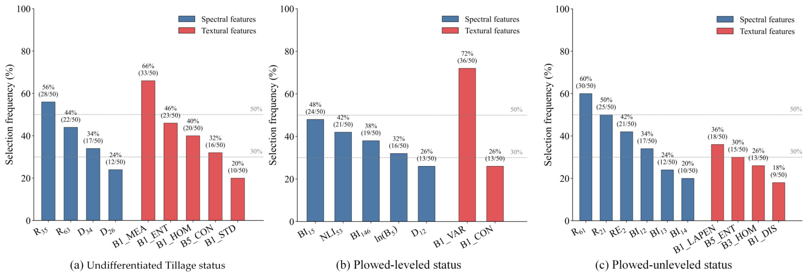
To further assess feature-selection stability, GA-based feature selection was repeated 50 times using different random seeds. The selection frequencies of the features in the final subsets were then calculated (Figure 11). Several features showed relatively high selection frequencies. These included R₃₅ and B1_MEA under the undifferentiated tillage status, B1_VAR under the plowed-leveled status, and R₆₁ and R₂₁ under the plowed-unleveled status. However, some selected features showed relatively low selection frequencies. This indicates that the GA-selected feature subsets had moderate stability. It also suggests that the final subsets may be influenced by the stochastic search process of GA.

3.5. SOM Retrieval Under Different Surface Tillage Statuses

3.5.1. SOM Retrieval Accuracy Under the Undifferentiated Tillage Status

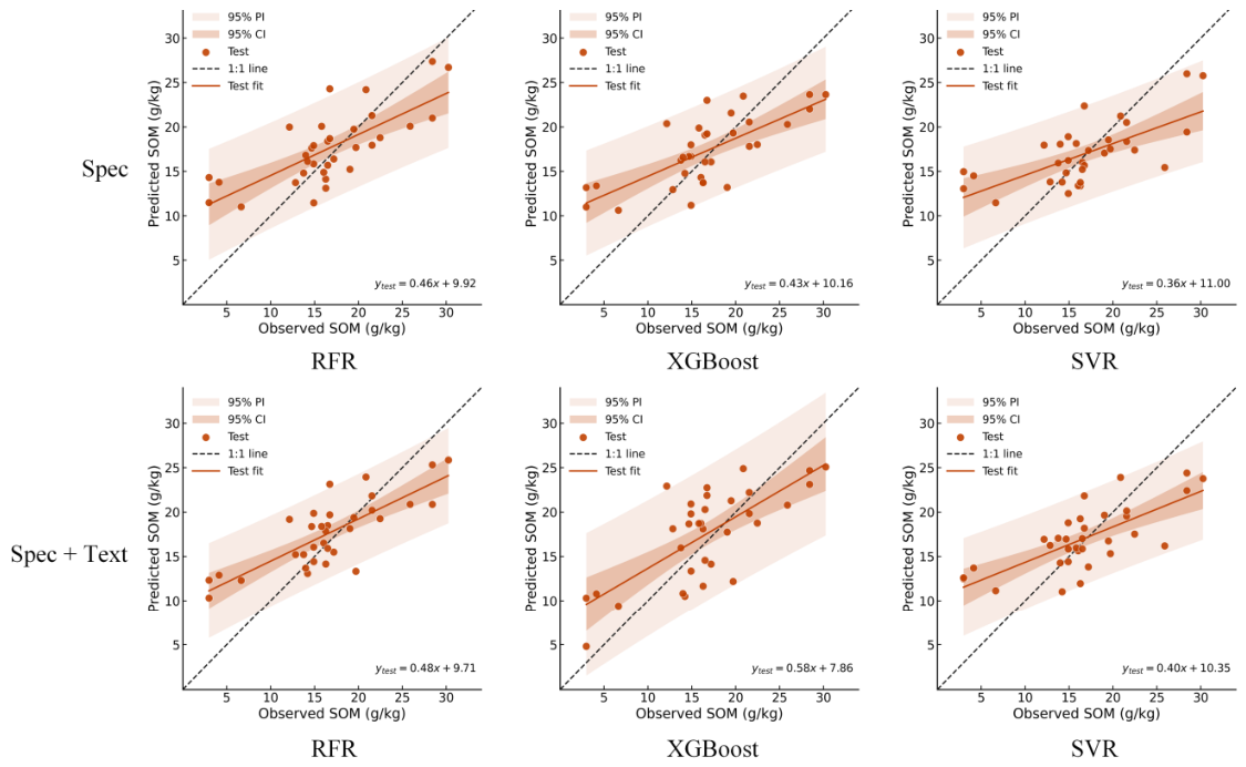
Under the undifferentiated tillage status, SOM retrieval results obtained with different input feature sets and models are presented in

Table 7. Statistics of SOM retrieval accuracy under different input features and algorithms for the undifferentiated tillage status.

Image Feature Fusion Method	Norm	Variable Name	Model	Test Set
				${\mathit{R}}^2$	rRMSE	LCCC	RPD
Spectral features	Spec	R35, R63, D34, D26	RFR	0.51	0.27	0.65	1.45
			SVR	0.43	0.29	0.56	1.35
			XGBoost	0.50	0.27	0.63	1.44
Fusion of spectral and textural features	Spec + Text	R35, R63, D34, D26, B1_MEA, B1_ENT, B1_HOM, B5_CON, B1_STD	RFR	0.57	0.26	0.69	1.54
			SVR	0.49	0.28	0.61	1.43
			XGBoost	0.50	0.27	0.70	1.44

. The incorporation of textural features improved the test-set accuracy metrics across all models. However, the magnitude of improvement varied among models. When only spectral features were used, the test-set $R^2$ values ranged from 0.43 to 0.51. The rRMSE values ranged from 0.27 to 0.29. The LCCC values ranged from 0.56 to 0.65. The RPD values ranged from 1.35 to 1.45. After textural features were incorporated, the test-set $R^2$ values increased to 0.49–0.57. The rRMSE values decreased to 0.26–0.28. The LCCC values increased to 0.61–0.70. The RPD values increased to 1.43–1.54.

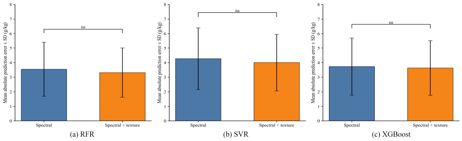
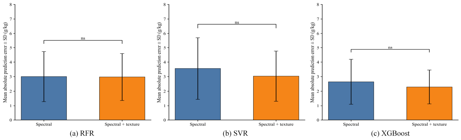
To further evaluate whether the texture-induced changes were statistically detectable, sample-level absolute prediction errors were compared between the spectral-only and spectral-plus-texture models (Figure 12). The mean absolute errors decreased slightly after textural features were incorporated for all three models. This was consistent with the overall improvement in test-set accuracy metrics. However, paired Wilcoxon tests showed that these reductions were not statistically significant (p ≥ 0.05). This indicates that, under the undifferentiated tillage status, the metric-level improvement from adding textural features did not translate into a statistically significant reduction in absolute prediction error. This may be related to the mixed surface conditions in the combined dataset.

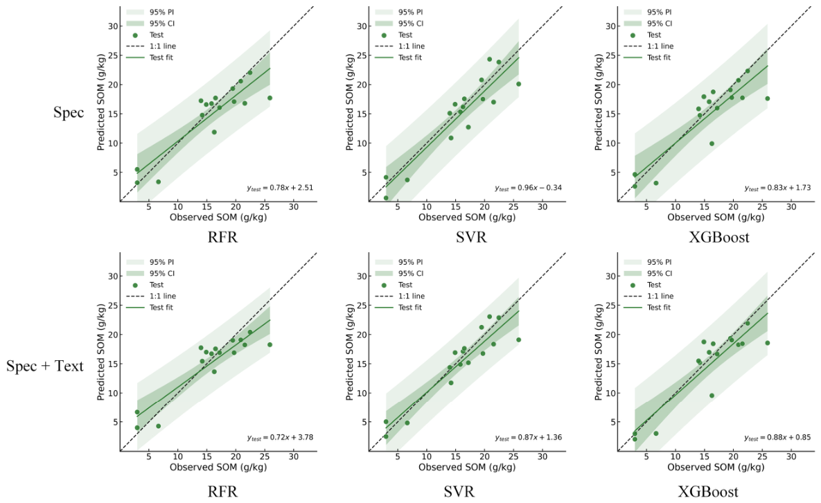
The scatter plots showed relatively wide dispersion around the 1:1 line for all models (Figure 13). The fitted lines for the test sets generally had slopes lower than 1. This pattern indicates a tendency to overestimate low SOM values and underestimate high SOM values.

3.5.2. SOM Retrieval Accuracy Under the Plowed-Leveled Status

Under the plowed-leveled status, the SOM retrieval results obtained using different feature sets and models are presented in

Table 8. Statistics of SOM retrieval accuracy across different input features and algorithms for the plowed-leveled status.

Image Feature Fusion Method	Norm	Variable Name	Model	Test Set
				${\mathit{R}}^2$	rRMSE	LCCC	RPD
Spectral features	Spec	BI15, NLI53, BI146, lnB5, D12	RFR	0.64	0.22	0.77	1.72
			SVR	0.53	0.25	0.67	1.50
			XGBoost	0.79	0.17	0.87	2.24
Fusion of spectral and textural features	Spec + Text	BI15, NLI53, BI146, lnB5, D12, B1_VAR, B1_CON	RFR	0.65	0.22	0.79	1.74
			SVR	0.55	0.25	0.73	1.53
			XGBoost	0.84	0.15	0.91	2.57

. When only spectral features were used, the test-set $R^2$ values ranged from 0.53 to 0.79. The rRMSE values ranged from 0.17 to 0.25. The LCCC values ranged from 0.67 to 0.87. The RPD values ranged from 1.50 to 2.24. After textural features were incorporated, the test-set $R^2$ values increased to 0.55–0.84. The rRMSE values decreased to 0.15–0.25. The LCCC values increased to 0.73–0.91. The RPD values increased to 1.53–2.57.

To evaluate whether the texture-induced changes were statistically detectable, sample-level absolute prediction errors were compared between the spectral-only and spectral-plus-texture models under the plowed-leveled status (Figure 14). The mean absolute errors generally decreased after textural features were incorporated. This was consistent with the improvement in test-set accuracy metrics. However, paired Wilcoxon tests showed that these reductions were not statistically significant (p ≥ 0.05). Therefore, under the plowed-leveled status, the improvement from textural features should be interpreted as a positive trend rather than a statistically confirmed reduction in absolute prediction error.

As shown in Figure 15, the scatter plots showed that the sample points were distributed closer to the 1:1 line than those under the undifferentiated tillage status. This pattern was more evident after textural features were incorporated. Among the tested models, XGBoost showed the best fit under the spectral-plus-texture setting.

3.5.3. SOM Retrieval Accuracy Under the Plowed-Unleveled Status

Under the plowed-unleveled status, the SOM retrieval results are presented in

Table 9. Statistics of SOM retrieval accuracy under different input features and algorithms for the plowed-unleveled status.

Image Feature Fusion Method	Norm	Variable Name	Model	Test Set
				${\mathit{R}}^2$	rRMSE	LCCC	RPD
Spectral features	Spec	R61, R21, RE2, BI12, BI13, BI14	RFR	0.77	0.20	0.87	2.16
			SVR	0.81	0.18	0.91	2.35
			XGBoost	0.75	0.20	0.87	2.07
Fusion of spectral and textural features	Spec + Text	R61, R21, RE2, BI12, BI13, BI14, B1_LAPEN, B5_ENT, B1_DIS, B3_HOM	RFR	0.80	0.18	0.88	2.29
			SVR	0.85	0.16	0.92	2.67
			XGBoost	0.77	0.20	0.88	2.14

. Retrieval accuracy under this status was generally the highest among the three tillage-status settings. It was also higher than that under the undifferentiated tillage status. When only spectral features were used, the test-set $R^2$ values ranged from 0.75 to 0.81. The rRMSE values ranged from 0.18 to 0.20. The LCCC values ranged from 0.87 to 0.91. The RPD values ranged from 2.07 to 2.35. After textural features were incorporated, the test-set $R^2$ values increased to 0.77–0.85. The rRMSE values decreased to 0.16–0.20. The LCCC values increased to 0.88–0.92. The RPD values increased to 2.14–2.67.

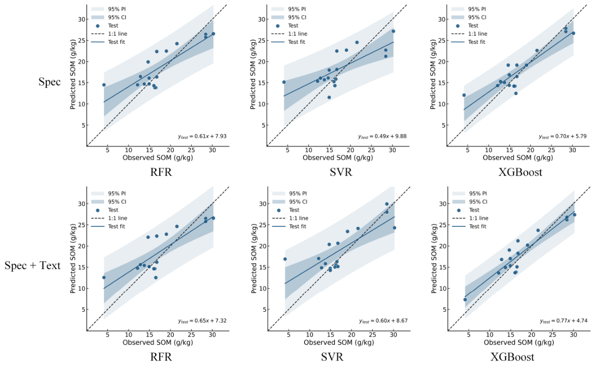
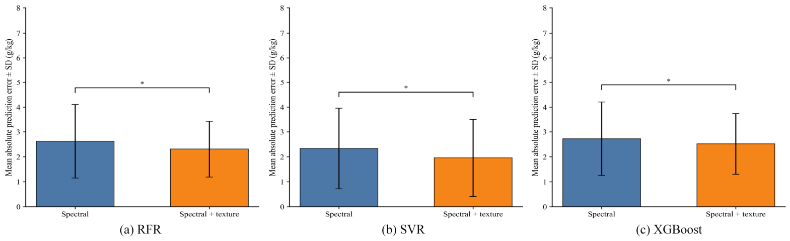
To evaluate whether the texture-induced changes were statistically detectable, sample-level absolute prediction errors were compared between the spectral-only and spectral-plus-texture models under the plowed-unleveled status (Figure 16). The mean absolute errors decreased after textural features were incorporated for all three models. This was consistent with the improvement in test-set accuracy metrics. Paired Wilcoxon tests showed significant reductions in absolute prediction errors (p < 0.05). This indicates that textural features provided a statistically detectable improvement in prediction error under the plowed-unleveled status.

The scatter plots showed that the test samples of all models were generally close to the 1:1 line under this status (Figure 17). The fitting relationships were also better than those under the undifferentiated tillage status. After textural features were incorporated, the SVR model showed the most concentrated point distribution and the best test-set fitting performance.

3.5.4. Comparison of Model Stability and Performance Differences

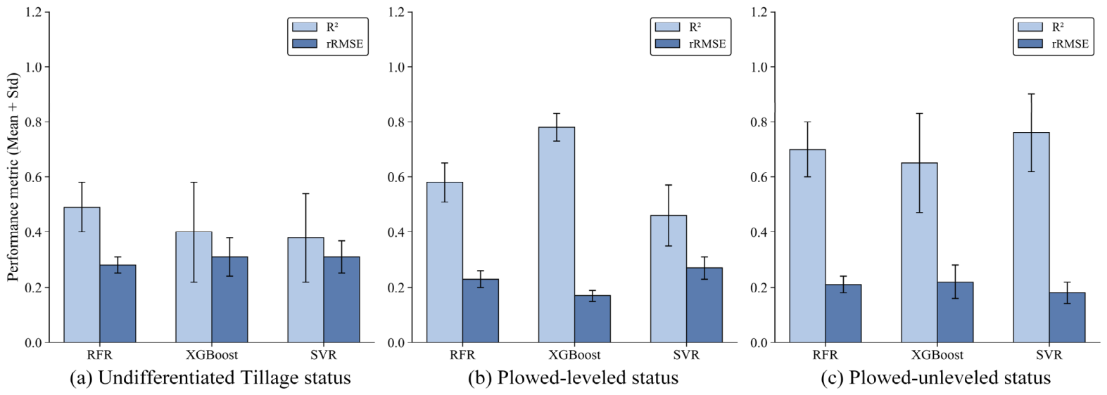
Figure 18 shows the five-fold cross-validation performance of the spectral-plus-texture models under different tillage-status settings. The mean values of $R^2$ and rRMSE were used to evaluate average model performance. The standard deviations were used to describe fold-to-fold variation and model stability. A smaller standard deviation indicated more stable model performance across different data partitions. Under the undifferentiated tillage status, RFR showed the best overall cross-validation performance. It had the highest mean $R^2$, the lowest mean rRMSE, and relatively small standard deviations. These results indicate better stability than the other models under this setting. Under the plowed-leveled status, XGBoost achieved the highest mean $R^2$ and the lowest mean rRMSE. It also showed small fold-to-fold variation. This indicates both high accuracy and stable performance under the plowed-leveled status. Under the plowed-unleveled status, SVR showed the best average cross-validation performance. It had the highest mean $R^2$ and the lowest mean rRMSE. Although its standard deviations were not the smallest among the three models, they remained within an acceptable range. This suggests that SVR achieved the best balance between predictive accuracy and stability under this status.

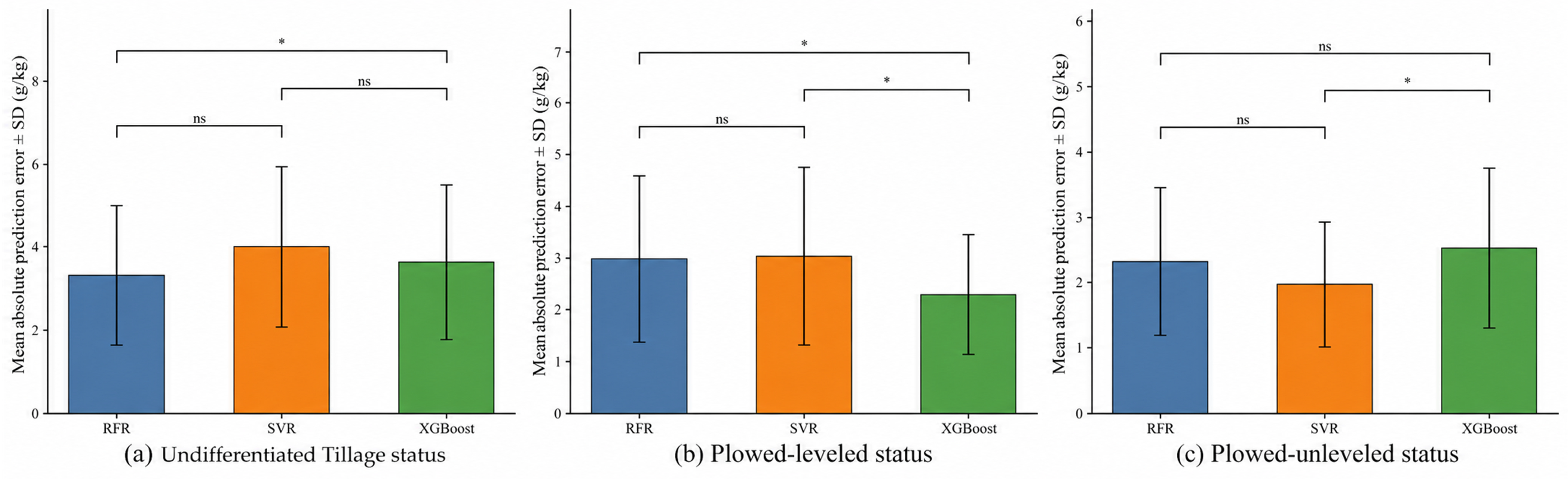
To further assess statistical differences in model performance, the mean absolute prediction errors of the spectral-plus-texture models were compared among RFR, XGBoost, and SVR using the held-out test sets (Figure 19). Under the undifferentiated tillage status, RFR had the lowest mean absolute prediction error. Only the difference between RFR and XGBoost was statistically significant. Under the plowed-leveled status, XGBoost had the lowest mean absolute prediction error. It was significantly different from both RFR and SVR. Under the plowed-unleveled status, SVR had the lowest mean absolute prediction error. It was significantly different from XGBoost, whereas its difference from RFR was not significant. Therefore, considering held-out test-set accuracy, five-fold cross-validation performance, and statistical comparisons of absolute prediction errors, RFR, XGBoost, and SVR were identified as the optimal models for the undifferentiated, plowed-leveled, and plowed-unleveled statuses, respectively.

3.6. Spatially Separated Leave-One-Zone-Out Validation

To examine the potential influence of spatial dependence in random sample-level splitting, LOZO validation was conducted for the optimal spectral-plus-texture model under each tillage-status setting. The LOZO results are provided in

Table A4. Spatially separated leave-one-zone-out validation results of the optimal spectral-plus-texture models under different tillage-status settings.

Surface Tillage Status	Model	Pooled LOZO				Fold-Wise Stability
		${\mathit{R}}^2$	rRMSE	LCCC	RPD	${\mathit{R}}^2$	rRMSE	LCCC	RPD
Undifferentiated tillage status	RFR	0.18	0.36	0.45	1.12	0.05 ± 0.30	0.38 ± 0.09	0.35 ± 0.18	1.03 ± 0.22
Plowed-leveled status	XGBoost	0.50	0.29	0.58	1.32	0.22 ± 0.35	0.31 ± 0.07	0.46 ± 0.18	1.24 ± 0.28
Plowed-unleveled status	SVR	0.64	0.27	0.73	1.68	0.38 ± 0.30	0.28 ± 0.06	0.62 ± 0.16	1.55 ± 0.35

Note: The four metrics under “Pooled LOZO” were calculated by pooling predictions from all left-out validation zones. The four metrics under “Fold-wise stability” are presented as mean ± SD across LOZO folds.

. Compared with the random-split test-set results, LOZO validation produced lower accuracy. This suggests that random sample-level splitting may provide optimistic estimates of cross-zone transferability. The fold-wise standard deviations were relatively large. This reflected variability among validation zones. It may also be partly related to the limited number of sampling zones and samples within each zone. Nevertheless, the status-specific models for the plowed-leveled and plowed-unleveled statuses still showed better pooled LOZO performance than the undifferentiated model. This suggests that status-specific modeling retained a relative advantage under the stricter spatially separated validation scheme.

4. Discussion

4.1. Effects of Tillage Status on Spectral Reflectance

This study showed that the relationship between SOM and spectral reflectance varied markedly among surface tillage statuses. Under the undifferentiated tillage status, the correlations between SOM and reflectance were generally weak across all bands. This may indicate that mixed surface conditions weakened the consistency of the SOM-related spectral response. The negative correlation observed under the plowed-leveled status was more consistent with the general spectral response pattern of SOM. Soil organic matter is mainly composed of humic substances. Humic acid and fulvic acid are important active components of these substances. Previous studies have shown that humic substances exhibit strong absorption across the visible to near-infrared regions. Therefore, soils with higher SOM content usually show lower reflectance [67,68,69]. In the plowed-leveled zones, the soil surface became relatively smooth after rotary tillage and mechanical leveling. Soil particles were finer, and the surface background was more uniform. These conditions may have reduced structural interference. They may also have allowed the SOM-related absorption response to be expressed more clearly. In contrast, the plowed-unleveled status showed significant positive SOM–reflectance correlations. This pattern deviated from the conventional negative relationship. It may be partly related to surface structural effects. The plowed-unleveled surfaces were characterized by large clods and ridge-furrow structures. The texture-derived indicators also showed higher Mean_STD, Mean_VAR, and Mean_ENT values than those of the plowed-leveled surfaces. Mean_HOM was lower under the plowed-unleveled status. These results indicate stronger local gray-level fluctuation, greater texture complexity, and lower homogeneity under this status. At the centimeter scale of UAV imagery, such structural heterogeneity can modify local illumination, shadow distribution, and scattering direction [68,70]. Therefore, reflectance may be influenced not only by soil chemical composition but also by surface structure and scattering background. This may partly explain why the SOM–reflectance relationship appeared statistically positive under the plowed-unleveled status. SNV transformation provided additional but indirect support for this interpretation. After SNV transformation, the positive correlations between SOM and several bands were weakened or reversed. This change was especially evident in the NIR band. Because SNV mainly reduces sample-wise spectral amplitude variation, these changes suggest that surface-structure-related amplitude effects may have contributed to the anomalous positive correlation. This interpretation is consistent with a previous study showing that SNV can reduce spectral amplitude variations associated with scattering and particle-size differences [49]. However, this result should not be interpreted as direct proof that physical surface roughness caused the positive correlation. Surface roughness was not independently measured in this study.

4.2. Integration of Spectral and Textural Features

In this study, incorporating textural features generally improved the overall test-set accuracy metrics of SOM retrieval. However, the statistical effect depended on surface tillage status. A significant reduction in absolute prediction error was mainly observed under the plowed-unleveled status. This suggests that textural features were more useful when surface structural heterogeneity was stronger. Under the undifferentiated tillage status, GA mainly selected ratio and difference features involving visible, red-edge, and NIR bands. These features describe reflectance contrasts between wavelength regions, rather than the magnitude of a single band. This is reasonable because SOM-related darkening is mainly expressed in the visible region. Red-edge and NIR reflectance can also be affected by soil scattering, particle arrangement, and surface structure [67,68,69,70]. Therefore, when plowed-leveled and plowed-unleveled surfaces were mixed, red–red-edge and visible–NIR contrast features may have been more useful than single-band reflectance [41,46,47]. The selected blue- and RedEdge2-band texture features described local brightness fluctuation, texture complexity, homogeneity, and contrast. However, in the mixed dataset, the same texture metric could represent SOM-related darkening, clod shadows, or smoothing effects. This may explain why texture improved the accuracy metrics but did not significantly reduce absolute prediction errors. Under the plowed-leveled status, the selected spectral features mainly included brightness, logarithmic, difference, and nonlinear red/red-edge contrast forms. On a relatively smooth surface, shadow and roughness effects were weaker. Soil color, albedo, and visible-to-red-edge contrast could therefore express SOM-related variation more consistently. The selected blue-band texture features represented residual local variance and contrast. Because the leveled surface had limited clod and shadow structures, these texture features provided only weak additional information. Under the plowed-unleveled status, GA selected ratio, reciprocal, and brightness features that emphasized reflectance amplitude and spectral contrast. These features may be useful when SOM signals are mixed with illumination differences and structure-related scattering. The selected texture features had clearer surface-structure relevance. Blue-band edge and dissimilarity features may reflect clod boundaries and shadow transitions. Red-band homogeneity may describe local smoothness. RedEdge2 entropy may represent complex gray-level variation over ridge-furrow microtopography [38,39,40,71]. Therefore, texture supplied surface-structure information that spectral indices alone could not fully represent. This led to a statistically detectable reduction in prediction error under the plowed-unleveled status. Overall, the 50 repeated GA runs showed moderate feature-selection stability. Thus, the selected features are physically reasonable empirical proxies under the present study conditions. They should not be treated as universal SOM indicators.

4.3. Differences in Model Adaptability to Tillage Statuses

The optimal model differed among tillage-status settings. RFR performed best under the undifferentiated tillage status. XGBoost performed best under the plowed-leveled status, whereas SVR performed best under the plowed-unleveled status. This indicates that model performance was affected by both input features and surface background [43,72,73]. When the two tillage statuses were combined, the spectral-textural response space became more heterogeneous. The same feature could represent SOM variation, shadow effects, or structure-related scattering. This weakened the feature–SOM relationship. Under this mixed condition, RFR was suitable because it builds multiple trees using bootstrap samples and random feature subsets. It then averages their predictions. This structure can reduce variance and improve robustness to noisy predictors [53]. Therefore, RFR was also used as the fitness estimator in the GA feature-selection procedure. After separating tillage statuses, the sample background became more consistent. This allowed other algorithms to fit status-specific relationships. Under the plowed-leveled status, roughness and shadow effects were weaker. The selected features therefore showed a clearer relationship with SOM. XGBoost could model nonlinear feature interactions through sequential tree boosting and regularization [54]. Under the plowed-unleveled status, the surface was rougher, and the spectral-textural response was more complex. SVR may be suitable because kernel mapping can fit nonlinear relationships under a limited sample size while controlling model complexity [55]. Using RFR as the GA fitness estimator may introduce some preference toward RFR-friendly features. However, the selected features were not evaluated only by RFR. They were further tested using RFR, XGBoost, and SVR. The fact that XGBoost and SVR became optimal under the two status-specific datasets suggests that the selected features were not exclusively dependent on RFR. However, algorithm-specific bias cannot be fully excluded [52]. Therefore, model selection in this study was based on a comprehensive judgment. It considered held-out test-set accuracy, five-fold cross-validation stability, and statistical comparisons of absolute prediction errors. Some numerical differences were not statistically significant. Thus, the optimal model should not be interpreted only as the model with the highest single accuracy value. Overall, no single algorithm was optimal across all tillage-status datasets. Under the present data conditions, model selection should be matched to the spectral-textural feature space shaped by surface tillage status.

4.4. Limitations, Transferability, Main Contributions, and Future Perspectives

4.4.1. Limitations and Transferability

This study has several limitations. First, the identification of the plowed-leveled and plowed-unleveled statuses mainly relied on field surveys, farming records, and visual interpretation of surface characteristics. This approach was sufficient for distinguishing broad surface conditions in this study. However, surface roughness was not directly measured using independent quantitative indicators. The lack of physical roughness metrics may affect the reproducibility of tillage-status classification. It may also limit the quantitative interpretation of roughness effects. Second, the two tillage-status groups were sampled from different zones. SOM, soil moisture proxy, clay content, silt content, and sand content showed no significant group differences. However, unmeasured management or soil-background factors may still have influenced bare-soil reflectance and model performance. Therefore, the observed tillage-status effects should be interpreted under the field conditions of this study. They should not be regarded as isolated tillage effects. Third, the SOM samples were mainly concentrated within 10–30 g/kg. Prediction reliability for very low or high SOM values remains uncertain.

Regarding transferability, the trained models and GA-selected feature combinations should be regarded as site-specific. The random-split results describe model performance under the present sampling population and data distribution. LOZO validation provides a stricter assessment of cross-zone prediction. Compared with random splitting, LOZO produced lower accuracy and noticeable fold-wise variability. This indicates that prediction for independent zones remains challenging. However, the status-specific models retained a relative advantage over the undifferentiated model. This suggests that tillage-status information remained useful under the present study conditions. For fields with similar arid bare-soil conditions, soil background, SOM range, and surface characteristics, the selected features and trained models may serve only as preliminary references. Local validation is still required. For each 500 m × 500 m target field or zone, at least one radiometrically calibrated UAV acquisition and approximately nine matched SOM samples are recommended for local validation or preliminary bias correction. If validation is unsatisfactory, feature selection and model training should be repeated using local UAV imagery and SOM samples. The same procedure is also recommended when local conditions differ substantially. For local status-specific model development, approximately 54 samples per major tillage status may be used as a practical lower reference. This value should not be treated as a universal threshold.

4.4.2. Main Contributions and Future Perspectives

Main Contributions. This study highlights the importance of tillage-induced surface heterogeneity in UAV-based SOM retrieval during the bare-soil period. The main contribution is that surface tillage status was explicitly incorporated into feature selection and model construction. The bare-soil background was therefore not treated as uniform. The results showed that SOM–reflectance relationships differed among tillage-status settings. They also showed that status-specific modeling achieved higher SOM retrieval accuracy than undifferentiated modeling under the present study conditions. In addition, textural features provided complementary surface-structure information. However, statistically detectable reductions in prediction error were mainly observed under the plowed-unleveled status. These findings provide a methodological reference for incorporating surface condition information into field-scale SOM estimation.

Future Perspectives. Future studies should further evaluate the transferability of this framework using independent datasets from different years, fields, or regions. If external datasets are available, the trained models should be tested directly. Otherwise, local calibration and validation datasets should be established. Stratified sampling should also be used to include more very low and high SOM samples. This would improve model reliability at the boundaries of the SOM range. Surface roughness should be measured quantitatively in future work. Possible methods include structure-from-motion photogrammetry and laser scanning. Useful indicators may include root mean square height and correlation length. A continuous roughness index could complement the discrete tillage-status classes used in this study. It may also support the development of unified models that include surface roughness as an explanatory variable.

5. Conclusions

Based on UAV multispectral imagery, this study compared SOM–remote sensing feature relationships, selected feature combinations, and machine learning model performance under three tillage-status settings during the bare-soil period. These settings included the undifferentiated tillage status, the plowed-leveled status, and the plowed-unleveled status. The main conclusions are as follows:

• The relationship between SOM and spectral reflectance differed among tillage-status settings. Under the undifferentiated tillage status, the correlations between SOM and reflectance were generally weak across all bands. Under the plowed-leveled status, SOM was generally significantly negatively correlated with spectral reflectance. In contrast, under the plowed-unleveled status, SOM was generally significantly positively correlated with spectral reflectance. Texture-derived heterogeneity indicators and SNV-based analysis suggested that this anomalous positive correlation may be partly associated with surface-structure-related spectral amplitude effects.
• Compared with spectral features alone, incorporating textural features improved the overall test-set accuracy metrics under all tillage-status settings. However, the reduction in absolute prediction error was statistically significant mainly under the plowed-unleveled status. This indicates that the contribution of textural features was dependent on surface tillage status.
• On the random-split held-out test set, status-specific modeling showed higher accuracy than undifferentiated modeling. The best models achieved test-set $R^2$ values of 0.57, 0.84, and 0.85 under the undifferentiated, plowed-leveled, and plowed-unleveled statuses, respectively. By jointly considering held-out test-set accuracy, five-fold cross-validation performance and stability, and statistical comparisons of absolute prediction errors, RFR, XGBoost, and SVR were identified as the optimal models for the undifferentiated, plowed-leveled, and plowed-unleveled statuses, respectively. LOZO validation further indicated that cross-zone transferability remains challenging. However, the status-specific models retained a relative advantage over the undifferentiated model.

Overall, incorporating tillage status into the analytical framework improved UAV-based SOM retrieval under the present study conditions. The results provide a methodological reference for field-scale SOM estimation during the bare-soil period. However, the status-specific models and GA-selected feature combinations developed in this study should be regarded as site-specific. Their application to other regions requires local recalibration and validation using representative UAV imagery, SOM samples, and tillage or surface-roughness information.

References

1. Murphy, B.W. Key Soil Functional Properties Affected by Soil Organic Matter—Evidence from Published Literature. IOP Conf. Ser. Earth Environ. Sci. 2015, 25, 012008. [Google Scholar]
2. Ou, J.; Wu, Z.; Yan, Q.; Feng, X.; Zhao, Z. Improving Soil Organic Carbon Mapping in Farmlands Using Machine Learning Models and Complex Cropping System Information. Environ. Sci. Eur. 2024, 36, 80. [Google Scholar] [CrossRef]
3. Li, T.; Cui, L.; Kuhnert, M.; McLaren, T.I.; Pandey, R.; Liu, H.; Wang, W.; Xu, Z.; Xia, A.; Dalal, R.C.; et al. A Comprehensive Review of Soil Organic Carbon Estimates: Integrating Remote Sensing and Machine Learning Technologies. J. Soils Sediments 2024, 24, 3556–3571. [Google Scholar] [CrossRef]
4. Guo, L.; Fu, P.; Shi, T.; Chen, Y.; Zhang, H.; Meng, R.; Wang, S. Mapping Field-Scale Soil Organic Carbon with Unmanned Aircraft System-Acquired Time Series Multispectral Images. Soil Tillage Res. 2020, 196, 104477. [Google Scholar]
5. Zhou, J.; Xu, Y.; Gu, X.; Chen, T.; Sun, Q.; Zhang, S.; Pan, Y. High-Precision Mapping of Soil Organic Matter Based on UAV Imagery Using Machine Learning Algorithms. Drones 2023, 7, 290. [Google Scholar] [CrossRef]
6. Zhang, H.; Wang, L.; Tian, T.; Yin, J. A Review of Unmanned Aerial Vehicle Low-Altitude Remote Sensing (UAV-LARS) Use in Agricultural Monitoring in China. Remote Sens. 2021, 13, 1221. [Google Scholar]
7. Yao, H.; Qin, R.; Chen, X. Unmanned Aerial Vehicle for Remote Sensing Applications—A Review. Remote Sens. 2019, 11, 1443. [Google Scholar] [CrossRef]
8. Milenković, M.; Karel, W.; Ressl, C.; Pfeifer, N. A Comparison of UAV and TLS Data for Soil Roughness Assessment. ISPRS Ann. Photogramm. Remote Sens. Spat. Inf. Sci. 2016, III-5, 145–152. [Google Scholar] [CrossRef]
9. Zhai, J.; Wang, N.; Hu, B.; Han, J.; Feng, C.; Peng, J.; Luo, D.; Shi, Z. Estimation of Soil Salinity by Combining Spectral and Texture Information from UAV Multispectral Images in the Tarim River Basin, China. Remote Sens. 2024, 16, 3671. [Google Scholar] [CrossRef]
10. Heil, J.; Jörges, C.; Stumpe, B. Fine-Scale Mapping of Soil Organic Matter in Agricultural Soils Using UAVs and Machine Learning. Remote Sens. 2022, 14, 3349. [Google Scholar] [CrossRef]
11. Reyes, J.; Wiedemann, W.; Brand, A.; Franke, J.; Ließ, M. Predictive Monitoring of Soil Organic Carbon Using Multispectral UAV Imagery: A Case Study on a Long-Term Experimental Field. Spat. Inf. Res. 2024, 32, 683–696. [Google Scholar] [CrossRef]
12. El-Jamaoui, I.; Delgado-Iniesta, M.J.; Martínez-Sánchez, M.J.; Pérez-Sirvent, C.; Martínez-López, S. Assessing Soil Organic Carbon in Semi-Arid Agricultural Soils Using UAVs and Machine Learning: A Pathway to Sustainable Water and Soil Resource Management. Sustainability 2025, 17, 3440. [Google Scholar] [CrossRef]
13. Wang, X.; Li, Y.-H.; Wang, R.-Y.; Shi, F.-Z.; Xu, S.-T. Remote sensing inversion of surface soil organic matter at jointing stage of winter wheat based on unmanned aerial vehicle multispectral. Chin. J. Appl. Ecol. 2020, 31, 2399–2406. [Google Scholar] [CrossRef]
14. Xie, S.; Wang, X.; Zhu, X.; Li, Y. Prediction of Soil Organic Matter Content in Winter Wheat Jointing Stage Based on UAV Multispectral and Machine Learning. Measurement 2025, 256, 118508. [Google Scholar] [CrossRef]
15. Xia, C.; Zhang, Y. Estimating Field-Scale Soil Organic Matter in Agricultural Soils Using UAV Hyperspectral Imagery. AgriEngineering 2025, 7, 339. [Google Scholar] [CrossRef]
16. Zhang, Y.; Luo, C.; Zhang, Y.; Gao, L.; Wang, Y.; Wu, Z.; Zhang, W.; Liu, H. Integration of Bare Soil and Crop Growth Remote Sensing Data to Improve the Accuracy of Soil Organic Matter Mapping in Black Soil Areas. Soil Tillage Res. 2024, 244, 106269. [Google Scholar] [CrossRef]
17. Shiratsuchi, L.; Ferguson, R.B.; Shanahan, J.F.; Adamchuk, V.I.; Rundquist, D.C.; Marx, D.B.; Slater, G.P. Water and Nitrogen Effects on Active Canopy Sensor Vegetation Indices. Agron. J. 2011, 103, 1815–1826. [Google Scholar] [CrossRef]
18. Li, F.; Mistele, B.; Hu, Y.; Chen, X.; Schmidhalter, U. Reflectance Estimation of Canopy Nitrogen Content in Winter Wheat Using Optimised Hyperspectral Spectral Indices and Partial Least Squares Regression. Eur. J. Agron. 2014, 52, 198–209. [Google Scholar] [CrossRef]
19. Segura, C.; Neal, A.L.; Castro-Sardiña, L.; Harris, P.; Rivero, M.J.; Cardenas, L.M.; Irisarri, J.G.N. Comparison of Direct and Indirect Soil Organic Carbon Prediction at Farm Field Scale. J. Environ. Manag. 2024, 365, 121573. [Google Scholar] [CrossRef]
20. Geng, J.; Tan, Q.; Lv, J.; Fang, H. Assessing Spatial Variations in Soil Organic Carbon and C:N Ratio in Northeast China’s Black Soil Region: Insights from Landsat-9 Satellite and Crop Growth Information. Soil Tillage Res. 2024, 235, 105897. [Google Scholar]
21. Wang, W.; Peng, J.; Zhu, W.; Yang, B.; Liu, Z.; Gong, H.; Wang, J.; Yang, T.; Lou, J.; Sun, Z. Study on Retrieval Method of Soil Organic Matter in Salinity Soil Using Unmanned Aerial Vehicle Remote Sensing. J. Geo-Inf. Sci. 2024, 26, 736–752. [Google Scholar]
22. Wang, Z.; Du, Z.; Li, X.; Bao, Z.; Zhao, N.; Yue, T. Incorporation of High Accuracy Surface Modeling into Machine Learning to Improve Soil Organic Matter Mapping. Ecol. Indic. 2021, 129, 107975. [Google Scholar] [CrossRef]
23. Zheng, G.; Chen, T.; Wang, Y.; Li, X.; Dai, W.; Xu, M.; Jiao, C.; Zhao, C. Rapid Monitoring of the Spatial Distribution of Soil Organic Matter Using Unmanned Aerial Vehicle Imaging Spectroscopy. Ann. GIS 2024, 30, 367–381. [Google Scholar] [CrossRef]
24. Yuan, J.; Gao, J.; Yu, B.; Yan, C.; Ma, C.; Xu, J.; Liu, Y. Estimation of Soil Organic Matter Content Based on Spectral Indices Constructed by Improved Hapke Model. Geoderma 2024, 443, 116823. [Google Scholar] [CrossRef]
25. Fanigliulo, R.; Antonucci, F.; Figorilli, S.; Pochi, D.; Pallottino, F.; Fornaciari, L.; Grilli, R.; Costa, C. Light Drone-Based Application to Assess Soil Tillage Quality Parameters. Sensors 2020, 20, 728. [Google Scholar] [CrossRef] [PubMed]
26. Zheng, X.; Jiang, T.; Li, X.; Ding, Y.; Zhao, K. The Temporal Variation of Farmland Soil Surface Roughness with Various Initial Surface States under Natural Rainfall Conditions. Soil Tillage Res. 2017, 170, 147–156. [Google Scholar] [CrossRef]
27. Croft, H.; Anderson, K.; Kuhn, N.J. Characterizing Soil Surface Roughness Using a Combined Structural and Spectral Approach. Eur. J. Soil Sci. 2009, 60, 431–442. [Google Scholar] [CrossRef]
28. Yuan, Z.; Wang, C.; Ma, H.; Liu, J.; Guo, Z.; Yao, C.; Wang, X.; Pan, X. UAV Hyperspectral Prediction of Soil Nutrients Using the Cluster-Hybrid Method. Comput. Electron. Agric. 2025, 237, 110534. [Google Scholar] [CrossRef]
29. Changji Hui Autonomous Prefecture People’s Government. Changji Hui Autonomous Prefecture Desertification Prevention and Control Plan (2021–2030). 2025. Available online: https://www.cj.gov.cn/p1/zfbwj/20250125/318237.html (accessed on 11 April 2026).
30. China Weather Network. Changji City Introduction. Available online: https://www.weather.com.cn/cityintro/101130401.shtml (accessed on 11 April 2026).
31. Xu, J.; Liu, Y.; Yan, C.; Yuan, J. Estimation of Soil Organic Matter Based on Spectral Indices Combined with Water Removal Algorithm. Remote Sens. 2024, 16, 2065. [Google Scholar] [CrossRef]
32. Changji City People’s Government. Statistical Communiqué of Changji City on the 2023 National Economic and Social Development. 2024. Available online: https://www.cjs.gov.cn/gk/lan/931604.htm (accessed on 11 April 2026).
33. Hutubi County People’s Government. Statistical Communiqué of Hutubi County on the 2023 National Economic and Social Development. 2024. Available online: https://www.htb.gov.cn/p222/tjgbtjj/20240528/296097.html (accessed on 11 April 2026).
34. Spiegel, H.; Dersch, G.; Hösch, J.; Baumgarten, A. Tillage effects on soil organic carbon and nutrient availability in a long-term field experiment in Austria. Die Bodenkult. 2007, 58, 47–58. [Google Scholar]
35. Martínez, I.; Chervet, A.; Weisskopf, P.; Sturny, W.G.; Etana, A.; Stettler, M.; Forkman, J.; Keller, T. Two decades of no-till in the Oberacker long-term field experiment: Part I. Crop yield, soil organic carbon and nutrient distribution in the soil profile. Soil Tillage Res. 2016, 163, 141–151. [Google Scholar]
36. NY/T 1121.6—2006; Soil Testing—Part 6: Determination of Soil Organic Matter. China Standards Press: Beijing, China, 2006.
37. Muñoz Sabater, J. ERA5-Land Hourly Data from 1950 to Present. Copernicus Climate Change Service (C3S) Climate Data Store (CDS). 2019. Available online: https://cds.climate.copernicus.eu/datasets/reanalysis-era5-land?tab=overview (accessed on 1 July 2026). [CrossRef]
38. Hall-Beyer, M. Practical Guidelines for Choosing GLCM Textures to Use in Landscape Classification Tasks over a Range of Moderate Spatial Scales. Int. J. Remote Sens. 2017, 38, 1312–1338. [Google Scholar] [CrossRef]
39. Warner, T. Kernel-Based Texture in Remote Sensing Image Classification. Geogr. Compass 2011, 5, 781–798. [Google Scholar]
40. Kupidura, P. The Comparison of Different Methods of Texture Analysis for Their Efficacy for Land Use Classification in Satellite Imagery. Remote Sens. 2019, 11, 1233. [Google Scholar] [CrossRef]
41. Zhao, M.-S.; Wang, T.; Lu, Y.-Y.; Wang, S.-H.; Wu, Y.-J. Improved Multivariate Modeling for Soil Organic Matter Content Estimation Using Hyperspectral Indexes and Characteristic Bands. PLoS ONE 2023, 18, e0286825. [Google Scholar] [CrossRef] [PubMed]
42. Liu, Y.; Sun, Q.; Huang, J.; Feng, H.-K.; Wang, J.-J.; Yang, G.-J. Estimation of Potato Above Ground Biomass Based on UAV Multispectral Images. Spectrosc. Spectr. Anal. 2021, 41, 2549–2555. [Google Scholar]
43. Forkuor, G.; Hounkpatin, O.K.L.; Welp, G.; Thiel, M. High Resolution Mapping of Soil Properties Using Remote Sensing Variables in South-Western Burkina Faso: A Comparison of Machine Learning and Multiple Linear Regression Models. PLoS ONE 2017, 12, e0170478. [Google Scholar] [CrossRef] [PubMed]
44. Rapinel, S.; Bouzillé, J.-B.; Oszwald, J.; Bonis, A. Use of bi-Seasonal Landsat-8 Imagery for Mapping Marshland Plant Community Combinations at the Regional Scale. Wetlands 2015, 35, 1043–1054. [Google Scholar] [CrossRef]
45. Shen, L.; Gao, M.; Yan, J.; Li, Z.-L.; Leng, P.; Yang, Q.; Duan, S.-B. Hyperspectral Estimation of Soil Organic Matter Content Using Different Spectral Preprocessing Techniques and PLSR Method. Remote Sens. 2020, 12, 1206. [Google Scholar] [CrossRef]
46. Song, B.; Park, K. Detection of Aquatic Plants Using Multispectral UAV Imagery and Vegetation Index. Remote Sens. 2020, 12, 387. [Google Scholar] [CrossRef]
47. Gupta, R.K. Comparative Study of AVHRR Ratio Vegetation Index and Normalized Difference Vegetation Index in District Level Agricultural Monitoring. Int. J. Remote Sens. 1993, 14, 53–73. [Google Scholar] [CrossRef]
48. Wang, L.; Zheng, S.; Liu, H.; Wang, X.; Meng, L.; Ma, Y.; Guan, H. Soil Organic Matter Inversion in Agro-Pastoral Ecotone of Northeast China. Soils 2022, 54, 184–190. [Google Scholar]
49. Barnes, R.J.; Dhanoa, M.S.; Lister, S.J. Standard Normal Variate Transformation and De-trending of Near-Infrared Diffuse Reflectance Spectra. Appl. Spectrosc. 1989, 43, 772–777. [Google Scholar]
50. Chen, Y.; Ma, L.; Yu, D.; Zhang, H.; Feng, K.; Wang, X.; Song, J. Comparison of Feature Selection Methods for Mapping Soil Organic Matter in Subtropical Restored Forests. Ecol. Indic. 2022, 135, 108545. [Google Scholar] [CrossRef]
51. Guo, H.; Zhang, R.; Dai, W.; Zhou, X.; Zhang, D.; Yang, Y.; Cui, J. Mapping Soil Organic Matter Content Based on Feature Band Selection with ZY1-02D Hyperspectral Satellite Data in the Agricultural Region. Agronomy 2022, 12, 2111. [Google Scholar] [CrossRef]
52. Kohavi, R.; John, G.H. Wrappers for Feature Subset Selection. Artif. Intell. 1997, 97, 273–324. [Google Scholar] [CrossRef]
53. Breiman, L. Random Forests. Mach. Learn. 2001, 45, 5–32. [Google Scholar] [CrossRef]
54. Chen, T.; Guestrin, C. XGBoost: A Scalable Tree Boosting System. In Proceedings of the 22nd ACM SIGKDD International Conference on Knowledge Discovery and Data Mining, San Francisco, CA, USA, 13–17 August 2016; ACM: New York, NY, USA, 2016; pp. 785–794. [Google Scholar]
55. Smola, A.J.; Schölkopf, B. A Tutorial on Support Vector Regression. Stat. Comput. 2004, 14, 199–222. [Google Scholar] [CrossRef]
56. Liu, J.; Jiang, L.; Yin, L.; Hu, H.; Wang, L.; Sun, J. Soil Nutrient Characteristics and Main Controlling Factors in the Oasis Zone of the Northeastern Margin of Tarim Basin. Northwest. Geol. 2023, 56, 141–152. [Google Scholar]
57. Bergstra, J.; Bengio, Y. Random Search for Hyper-Parameter Optimization. J. Mach. Learn. Res. 2012, 13, 281–305. [Google Scholar]
58. Kohavi, R. A Study of Cross-Validation and Bootstrap for Accuracy Estimation and Model Selection. In Proceedings of the 14th International Joint Conference on Artificial Intelligence, Montreal, QC, Canada, 20–25 August 1995; Morgan Kaufmann: San Francisco, CA, USA, 1995; Volume 2, pp. 1137–1143. [Google Scholar]
59. Chicco, D.; Warrens, M.J.; Jurman, G. The Coefficient of Determination R-Squared Is More Informative than SMAPE, MAE, MAPE, MSE and RMSE in Regression Analysis Evaluation. PeerJ Comput. Sci. 2021, 7, e623. [Google Scholar] [CrossRef] [PubMed]
60. Saldaña-Villota, T.M.; Cotes-Torres, J.M. Comparison of Statistical Indices for the Evaluation of Crop Models Performance. Rev. Fac. Nac. Agron. Medellín 2021, 74, 9675–9684. [Google Scholar] [CrossRef]
61. Li, H.; Liang, Z.; Chen, Y.; Liu, H.; Wang, J.; Xu, B.; Huang, W. Prediction of Soil Organic Carbon in a New Target Area by Near-Infrared Spectroscopy: Comparison of the Effects of Spiking in Different Scale Soil Spectral Libraries. Sensors 2020, 20, 4357. [Google Scholar] [CrossRef] [PubMed]
62. Lin, L.I.-K. A Concordance Correlation Coefficient to Evaluate Reproducibility. Biometrics 1989, 45, 255–268. [Google Scholar] [CrossRef] [PubMed]
63. Cui, X.; Han, W.; Dong, Y.; Zhai, X.; Ma, W.; Zhang, L.; Huang, S. Estimating and Mapping Soil Salinity in Multiple Vegetation Cover Periods by Using Unmanned Aerial Vehicle Remote Sensing. Remote Sens. 2023, 15, 4400. [Google Scholar] [CrossRef]
64. Roberts, D.R.; Bahn, V.; Ciuti, S.; Boyce, M.S.; Elith, J.; Guillera-Arroita, G.; Hauenstein, S.; Lahoz-Monfort, J.J.; Schröder, B.; Thuiller, W.; et al. Cross-validation Strategies for Data with Temporal, Spatial, Hierarchical, or Phylogenetic Structure. Ecography 2017, 40, 913–929. [Google Scholar] [CrossRef]
65. Bowers, S.A.; Hanks, R.J. Reflection of Radiant Energy from Soils. Soil Sci. 1965, 100, 130–138. [Google Scholar] [CrossRef]
66. Lobell, D.B.; Asner, G.P. Moisture Effects on Soil Reflectance. Soil Sci. Soc. Am. J. 2002, 66, 722–727. [Google Scholar] [CrossRef]
67. Ben-Dor, E.; Banin, A. Near-Infrared Analysis as a Rapid Method to Simultaneously Evaluate Several Soil Properties. Soil Sci. Soc. Am. J. 1995, 59, 364–372. [Google Scholar]
68. Stenberg, B.; Viscarra Rossel, R.A.; Mouazen, A.M.; Wetterlind, J. Visible and Near Infrared Spectroscopy in Soil Science. In Advances in Agronomy; Sparks, D.L., Ed.; Academic Press: San Diego, CA, USA, 2010; Volume 107, pp. 163–215. [Google Scholar]
69. Ribeiro, S.G.; Oliveira, M.R.R.D.; Lopes, L.M.; Costa, M.C.G.; Toma, R.S.; Araújo, I.C.S.; Moreira, L.C.J.; Teixeira, A.S. Reflectance Spectroscopy in the Prediction of Soil Organic Carbon Associated with Humic Substances. Rev. Bras. Cienc. Solo 2023, 47, e0220143. [Google Scholar] [CrossRef]
70. Cierniewski, J. A Model for Soil Surface Roughness Influence on the Spectral Response of Bare Soils in the Visible and Near-Infrared Range. Remote Sens. Environ. 1987, 23, 97–115. [Google Scholar] [CrossRef]
71. Haralick, R.M.; Shanmugam, K.; Dinstein, I. Textural Features for Image Classification. IEEE Trans. Syst. Man Cybern. 1973, SMC-3, 610–621. [Google Scholar] [CrossRef]
72. Lima, A.A.J.; Lopes, J.C.; Lopes, R.P.; de Figueiredo, T.; Vidal-Vázquez, E.; Hernández, Z. Soil Organic Carbon Assessment Using Remote-Sensing Data and Machine Learning: A Systematic Literature Review. Remote Sens. 2025, 17, 882. [Google Scholar] [CrossRef]
73. Angelopoulou, T. Soil Reflectance Spectroscopy for Supporting Sustainable Development Goals. In Information and Communication Technologies for Agriculture—Theme I: Sensors; Bochtis, D.D., Lampridi, M., Petropoulos, G.P., Ampatzidis, Y., Pardalos, P., Eds.; Springer: Cham, Switzerland, 2022; Volume 182, pp. 17–42. [Google Scholar]
Figure 1. Location and overview of the study area.
Drones 10 00516 g001
Figure 3. Field photographs of different tillage statuses during the bare-soil period in the study area: (a) plowed-unleveled status; (b) plowed-leveled status.
Drones 10 00516 g003
Figure 4. DJI M300 RTK unmanned aerial vehicle equipped with a YUSENSE MS600 Pro multispectral camera.
Drones 10 00516 g004
Figure 5. Distribution and descriptive statistics of SOM samples in the training and test sets. (a) Stacked distribution of sample numbers across different SOM classes; (b) Mean SOM content ± standard deviation (Mean ± SD). Note: ns, not significant based on the Mann–Whitney U test (p ≥ 0.05). Abbreviations: Undiff., undifferentiated tillage status; Unlev., plowed-unleveled status; Lev., plowed-leveled status.
Drones 10 00516 g005
Figure 6. Bar chart of Pearson correlation coefficients between SOM and spectral reflectance under different tillage statuses. Note: *** indicate significance at the 0.001 level; ns indicates no significant correlation.
Drones 10 00516 g006
Figure 7. Bar charts of Pearson correlation coefficients (|R|) between SOM and spectral and textural features under the undifferentiated tillage status. (a) Top 40 spectral features; (b) Top 20 textural features. Note: *, **, and *** indicate significance at the 0.05, 0.01, and 0.001 levels, respectively; ns indicates no significant correlation.
Drones 10 00516 g007
Figure 8. Bar charts of Pearson correlation coefficients (|R|) between SOM and spectral and textural features under the plowed-unleveled status. (a) Top 40 spectral features; (b) Top 20 textural features. Note: *, **, and *** indicate significance at the 0.05, 0.01, and 0.001 levels, respectively; ns indicates no significant correlation.
Drones 10 00516 g008
Figure 9. Bar charts of Pearson correlation coefficients (|R|) between SOM and spectral and textural features under the plowed-leveled status. (a) Top 40 spectral features; (b) Top 20 textural features. Note: *, **, and *** indicate significance at the 0.05, 0.01, and 0.001 levels, respectively.
Drones 10 00516 g009
Figure 10. SNV-based supporting analysis under the plowed-unleveled status. (a) Mean original reflectance spectra and (b) mean SNV-transformed spectra of SOM subgroups divided by the median SOM value; shaded areas indicate ±SD. (c) Pearson correlations between SOM and raw reflectance or SNV-transformed spectral values. Note: Asterisks above bars indicate the significance of individual correlations, whereas asterisks associated with Δr indicate the significance of SNV-induced changes in correlation coefficients tested by paired bootstrap resampling. *, **, and *** indicate significance at p < 0.05, p < 0.01, and p < 0.001, respectively; ns indicates no significance.
Drones 10 00516 g010
Figure 11. Stability of GA-based feature selection under different surface tillage-status groups. Note: Values above bars indicate selection percentages and counts. Dashed gray lines indicate 30% and 50% selection-frequency thresholds.
Drones 10 00516 g011
Figure 12. Comparison of mean absolute prediction errors between spectral-only and spectral-plus-texture models under the undifferentiated tillage status. Error bars indicate ±SD. Significance was tested using paired Wilcoxon signed-rank tests. ns, p ≥ 0.05.
Drones 10 00516 g012
Figure 13. Scatter plots of predicted versus observed SOM values under different input features (Spec, Spec + Text) and algorithms (RFR, XGBoost, SVR) for the undifferentiated tillage status.
Drones 10 00516 g013
Figure 14. Comparison of mean absolute prediction errors between spectral-only and spectral-plus-texture models under the plowed-leveled status. Error bars indicate ±SD. Significance was tested using paired Wilcoxon signed-rank tests. ns, p ≥ 0.05.
Drones 10 00516 g014
Figure 15. Scatter plots of predicted versus observed SOM values under different input features (Spec, Spec + Text) and algorithms (RFR, XGBoost, SVR) for the plowed-leveled status.
Drones 10 00516 g015
Figure 16. Comparison of mean absolute prediction errors between spectral-only and spectral-plus-texture models under the plowed-unleveled status. Error bars indicate ±SD. Significance was tested using paired Wilcoxon signed-rank tests. * p < 0.05.
Drones 10 00516 g016
Figure 17. Scatter plots of predicted versus observed SOM values under different input features (Spec, Spec + Text) and algorithms (RFR, XGBoost, SVR) for the plowed-unleveled status.
Drones 10 00516 g017
Figure 18. Cross-validation performance and stability of spectral-plus-texture SOM retrieval models under different tillage statuses.
Drones 10 00516 g018
Figure 19. Comparison of mean absolute prediction errors among spectral-plus-texture models under different tillage statuses. Error bars indicate ±SD. Significance was tested using paired Wilcoxon signed-rank tests. * p < 0.05; ns, p ≥ 0.05.
Drones 10 00516 g019