Effectiveness Comparison of Selected 3D Tracking Controllers for Underactuated UUVs with Small Displacement of Mass Center

Highlights

What are the main findings?

• Comparison of the effectiveness of selected control schemes for an underwater vehicle described by a five-DOF model in the case of a small shift of the center of mass.
• Simulation tests were performed under defined operating conditions to ensure comparable results. The tested model represented an underwater vehicle used in real marine research, taking into account the capabilities of its propulsion engines.

What are the implications of the main findings?

• The obtained simulation results allow for estimating the vehicle’s behavior when a given type of control scheme is used and small shifts of the center of mass occur (of the order of 1–1.5 cm), which enables the assessment of the usefulness of such a scheme.
• Using the presented method of testing control algorithms, a decision can be made already at the stage of numerical analysis whether to undertake experimental tests on a real vehicle or to abandon them, thus reducing the costs and expenditure on research work.

Abstract

This work is devoted a particular trajectory tracking problem of underactuated unmanned underwater vehicles (UUVs) with model reduced to five degrees of freedom (DOF). Such a model is quite widespread in the literature and used to describe the dynamics of UUVs. On this basis, various control strategies are designed, such that the closed-loop system track the trajectory with assumed accuracy. Unfortunately, the main drawback of this approach is that the presented results relate to the situation when the center of the mass is the same as the geometric center-point. Several algorithms have been selected for testing the control effectiveness (one based on the model with shifted center of the mass and other four based on the assumption that this center is in the same place as the geometric center). The goal of the paper is to check whether the correction mechanisms contained in the controller ensure the implementation of the trajectory tracking task. Simulation results on the five-DOF vehicle model show performance of the considered control schemes in the presence of a small shift of the mass center.

1. Introduction

Interest in the use of underwater vehicles for exploration of water reservoirs has been around for many years. Vehicles, in particular autonomous underwater vehicles (AUVs), can perform various tasks, and one of these tasks is trajectory tracking. However, before designing the control strategy, it is necessary to build a vehicle dynamics model. This article pays attention to one of the issues, namely obtaining a preliminary answer to the question whether known algorithms can work effectively when a slight movement of the center of mass occurs. The test is devoted only to underactuated vehicles because for them, the construction of the appropriate control scheme is a big challenge.

Typically used submarine models in research have six DOF, so they are quite complex due to the fact that not only the center of mass can be shifted, but also various physical phenomena occur, including external disturbances and internal couplings, e.g., [1,2]. Such models are used to design the trajectory tracking scheme, for example in [3] (the model predictive control (MPC) method based on the disturbance observer), in [4] (fuzzy logic together with the Lyapunov function of the integral barrier) and in [5] (use of a neural network for an underwater vehicle with input saturation control).

With some conditions, as indicated in [2], the model can be simplified to five DOF. However, over time, many works have appeared using this model to carry out the trajectory tracking task. One of the reasons is certainly the fact that control strategies based on such a model are also less complex from a mathematical point of view.

The first group consists of the so-called classical methods, which use combinations of known methods to control marine vehicles. In many works, the use of backstepping is proposed with other approaches. In [6], this method was applied for the realization of integrated guidance and control tasks. The strategies proposed in [7,8] are composed of the backstepping plus bioinspired neurodynamics model, in [9] of backstepping, the neural dynamics model together with the SMC (sliding mode control), in [10] of backstepping and the observer of predefined time disturbance, in [11] of backstepping and the active disturbance rejection control (ADRC) method, and in [12] of backstepping and adaptive fixed time controller. A combination of backstepping with an event-triggered approach was considered in [13] and backstepping with an integral SMC scheme in [14]. The application of a strategy based on backstepping with adaptive SMC was given in [15], whereas the use of backstepping and a fixed-time disturbance observer of disturbances was shown in [16].

The second group of methods are those that use learning-based techniques. A common solution to perform the trajectory tracking task is the use of neural networks (NN) together with other control methods. For example, ref. [17] can be mentioned here, in which, in addition to NN, the dynamic surface control (DSC) method was applied, or [18], in which non-singular terminal sliding mode control and adaptive techniques were used. In [19], the line-of-sight (LOS) tracking controller with NN, in [20], a model-data-driven learning adaptive robust control (LARC) strategy with the feedforward compensation-line-of-sight (FFC-LOS) guidance law, and in [21], backstepping with NN are employed. The application of the NN radial basis function (RBFNN) with the event-triggered method can be found in [22], the deep neural network (DNN), the event-triggered method, and the nonlinear model predictive control (NMPC) in [23], predefined time adaptive control and RBFNN in [24], RBFNN with adaptive dynamic programming in [25], while RBFNN with prescribed performance control and an event-triggered mechanism in [26]. In [27], a robust fixed-time control strategy with NN disturbance observer was proposed. This group also includes alternative methods for robust control that can potentially be used in AUV control. For example, in [28], a combination of reinforcement learning and a neural network was applied for the follow-up of the path and in [29], where a framework incorporating genetic programming (GP) with a novel population initialization method was proposed.

There are also methods that would be difficult to classify into the previously mentioned groups because they combine various techniques that are perhaps less popular. For example, a non-singular terminal sliding mode together with active disturbance rejection decoupling control (NTSM-ADRDC) [30], a prescribed performance controller with LOS and an event-triggered mechanism [31], LOS together with the DSC technique [32], application of the proportional–integral–derivative (PID) controller and SMC [33], an integral time-delay SMC which divided the input of vehicle model into cascade system model (composed of kinematics and dynamics subsystem) [34].

Publications related to trajectory tracking, which confirmed the effectiveness of algorithms based on the dynamics model by five DOF, are not many. The results of the real experiments are shown in [35], but the vehicle was shifted only slightly more than 0.5 cm on the vertical axis. The tests presented in [36] focused on avoiding obstacles, which does not quite match the issues considered here. The work [37] contained results for a control strategy based on a model with a diagonal inertia matrix, and therefore the model was simplified. Tracking errors for some variables indicated some inaccuracies, i.e., the algorithm acted only partially effectively. Other publications, i.e., ref. [38], presented only the results of the HIL test (hardware-in-the-loop) and not tests performed in maritime conditions. Simulation tests can be concluded to be necessary because their results may be used for real experiments in the future.

Publications proposing new control schemes for a five-DOF model typically include simulation results and only exceptionally include experimental results from a real vehicle. In five-DOF models, the inertia matrix is assumed to be diagonal. Therefore, the control algorithm is assumed to be sufficiently effective to ensure that even in the presence of motion disturbances (external or resulting from model inaccuracies), the task of tracking the desired trajectory can be achieved. To ensure correct algorithm performance, a disturbance term is added to enable more accurate task realization. To confirm the controller’s effectiveness, mathematically complex trajectories are often tested. The authors emphasize the benefits of using the proposed control scheme, often comparing their results with those obtained using competitive methods. One possible disturbance to vehicle motion is a sudden (or permanent) shift of the center of mass relative to the geometric center. An effective controller should incorporate a mechanism to address this problem. Unfortunately, many algorithms have been observed to fail in such situations. However, the possibility of such a change poses a real threat. This article attempts to verify the effectiveness of several selected control algorithms in the presence of a center of mass shift using simulation tests. There is another problem: the suitability of known control schemes for trajectory tracking under various operating conditions. Some algorithms, although effective under the conditions indicated by the authors, do not work under modified operating conditions and are therefore not universal, even to a limited extent. In the proposed paper, conditions were modified from those adopted in the source publications, taking into account the actual capabilities of the drives, as determined by data from the literature.

The main purpose of the paper is to draw attention to the fact that the trajectory tracking control based on a widely used five-DOF model with a diagonal inertia matrix may prove to be useless when the dynamic parameters of the vehicle or the working conditions change. Moreover, assuming a real limitation of the vehicle’s driving forces and torques may worsen the efficiency of the controller. Only one aspect is considered here, namely a slight displacement of the center of mass, which may result from inaccurate measurement or an unexpected reason (e.g., changes in dynamic parameters during movement).

The contributions of the work are as follows.

• Comparison of the effectiveness of controlling five trajectory tracking schemes known from the literature. The first of them is based on a model with a symmetric inertia matrix by five DOF, while the others on the model have a diagonal matrix. The goal is to show how robust the schemes are when there is a slight shift of the center of the mass (by 1–1.5 cm).
• In contrast to [39], the vehicle model has been changed (other model parameters), but an underwater vehicle was chosen, which is used in tests at sea. In addition, the investigation includes the real values of forces and torques, which can be obtained by carrying out the task of tracking the trajectory. The operating conditions of the control scheme and the value of the displacement of the mass were also changed. An important problem is to check the suitability of the control strategy for a vehicle different from the one in the source work and for changed operating conditions.
• Analysis of the results received from the simulation and the restrictions that arise for each selected method of tracking the trajectory and commenting on its usability.

The presented method of comparing control schemes can be particularly useful at the stage of their design and when analyzing their performance, when the center of the mass is moved relative to the geometric center of the vehicle. Based on the presented approach, one can decide whether one’s own strategy will be further developed or whether it is worth modifying without performing the real experiment.

The remainder of the paper is organized as follows. In Section 2, equations of motion of the model of an underwater vehicle are presented. The selected control tracking schemes are given in Section 3. Section 4 shows simulations concerning all control strategies under consideration and contains a discussion of the results. Section 5 offers conclusions. Additional information is included in Appendix A.

2. Equations of Motion of Underwater Vehicle

Underactuated Marine Vehicle Model

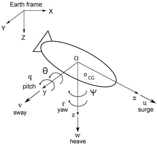
The model under consideration is presented in Figure 1.

Figure 1. Underactuated underwater vehicle in the coordinate systems (earth and body).

The variables describing position and orientation are defined by $\eta ={[x,y,z,\theta ,\psi ]}^T$ and the kinematic and dynamic equations are [1]:

$$\begin{array}{ccc}\hfill & & \dot{\eta }=J\left(\eta \right)\nu ,\hfill \end{array}$$

(1)

$$\begin{array}{ccc}\hfill & & M\dot{\nu }=-H(\nu ,\eta )+\tau +{\tau }_e,\hfill \end{array}$$

(2)

where $\nu ={[u,v,w,q,r]}^T$ is the vector of linear and angular velocities, $\tau ={[{\tau }_u,0,0,{\tau }_q,{\tau }_r]}^T$ is the vector of control input signals, and ${\tau }_e={[{\tau }_{eu},{\tau }_{ev},{\tau }_{ew},{\tau }_{eq},{\tau }_{er}]}^T$ is the vector of environmental disturbances (eventually also including unknown dynamics). The meaning of the other symbols are explained in Appendix A. Based on the results given in Appendix A, Equation (2) may be rewritten as

$$\begin{array}{ccc}\hfill & & m_{11}\dot{u}=m_{22}vr-m_{33}wq-d_{11}u+{\tau }_u+({\tau }_{eu}-m_{15}\dot{q}+{\Delta }_1),\hfill \end{array}$$

(3)

$$\begin{array}{ccc}& & m_{22}\dot{v}=-m_{11}ur-d_{22}v+({\tau }_{ev}-m_{26}\dot{r}+{\Delta }_2),\hfill \end{array}$$

(4)

$$\begin{array}{ccc}& & m_{33}\dot{w}=m_{11}uq-d_{33}w+({\tau }_{ew}-m_{35}\dot{q}+{\Delta }_3),\hfill \end{array}$$

(5)

$$\begin{array}{ccc}& & m_{55}\dot{q}=(m_{33}-m_{11})uw-d_{55}q-z_{g}Ws\theta +{\tau }_q+({\tau }_{eq}-(m_{15}\dot{u}+m_{35}\dot{w})+{\Delta }_5),\hfill \end{array}$$

(6)

$$\begin{array}{ccc}\hfill & & m_{66}\dot{r}=(m_{11}-m_{22})uv-d_{66}r+{\tau }_r+({\tau }_{er}-m_{26}\dot{v}+{\Delta }_6).\hfill \end{array}$$

(7)

From Equations (3)–(7), it follows that the components resulting from mechanical couplings originating from the displacement of the vehicle’s center of mass ($m_{15},m_{26},$ and $m_{35}$) cause the disturbance functions to have larger values. These are no longer only initial disturbances, but additional moments of forces arising in the absence of symmetry of the vehicle. The simplified model, that is, without omitting the effect of mechanical couplings in the last component (in brackets), contains only disturbances ${\tau }_{eu},{\tau }_{ev},{\tau }_{ew},{\tau }_{eq},$ and ${\tau }_{er}$.

Comment. From Equations (3)–(7) it follows that the total disturbance components can be expressed as follows:

$$\begin{array}{ccc}\hfill & & {\tau }_{d1}={\tau }_{eu}-m_{15}\dot{q}+{\Delta }_1,{\tau }_{d2}={\tau }_{ev}-m_{26}\dot{r}+{\Delta }_2,{\tau }_{d3}={\tau }_{ew}-m_{35}\dot{q}+{\Delta }_3,\hfill \end{array}$$

(8)

$$\begin{array}{ccc}& & {\tau }_{d5}={\tau }_{eq}-(m_{15}\dot{u}+m_{35}\dot{w})+{\Delta }_5,{\tau }_{d6}={\tau }_{er}-m_{26}\dot{v}+{\Delta }_6.\hfill \end{array}$$

(9)

Therefore, if disturbances are taken into account in the vehicle model, the controller should respond appropriately when they occur.

Justification for using model (1)–(7). The model under consideration describes the dynamics of the vehicle taking into account the shift of the center of mass. It is a five-DOF model reduced to a well-known six-DOF model, e.g., from [1,2]. The effectiveness of five-DOF models that incorporate a perturbation component has been extensively tested. Among the works listed in the references, the following can be mentioned [10,12,13,16,19,22,25,26,27,38].

It should be noted that the model with a diagonal inertia matrix was used in experimental studies. For example, in [37], external disturbances were included (in the five-DOF model, the seawater experiment in the port), and in [40,41], disturbances were omitted (four-DOF model, engineering basin experiment), ref. [42] (four-DOF model, a real-time controller implementation). In turn, ref. [43] shows the results of a sea test for a six-DOF vehicle (ignoring model disturbances).

3. Selected Trajectory Tracking Control Schemes

For comparative tests, taking into account the suitability for small displacements, five control schemes were selected, which are given below. Explanation of symbols used in the equations is given in Abbreviations.

The aim of the theoretical analysis is to estimate based on general equations describing the control strategy’s robustness to a possible shift in the center of mass of the underwater vehicle. Strategies are most often designed considering a vehicle model without inertial couplings. However, in a real vehicle, a situation may arise in which the model should be described by a symmetric inertia matrix. A control scheme dedicated to the model with a shifted center of mass and four for the model without such a shift were selected for analysis.

3.1. Velocity Transformation-Based Algorithm (VTBA)

Model and Initial Assumption. The tracking control scheme was proposed in [39]. Both the vehicle model and the appropriate algorithm concern a situation in which the center of mass does not have to be identical to the geometric center. Therefore, Equations (3)–(7) refer to the description of the dynamics. The desired velocities are assumed in a general form (needed for the kinematic controller):

$$\begin{array}{ccc}\hfill & & {\mu }_{du}=f_{11}({\zeta }_1,{\psi }_e,x_e),{\mu }_{dq}=f_{12}({\zeta }_2,z_e,{\psi }_e,{\theta }_e),{\mu }_{dr}=f_{13}({\zeta }_3,y_e,{\psi }_e).\hfill \end{array}$$

(10)

The input signals after velocity transformation are (in the dynamic controller):

$$\begin{array}{ccc}\hfill & & {\tau }_u=f_{u1}({\zeta }_{u1}\left(\widehat{p}\right),{\widehat{\tau }}_{eu},x_g,z_g,{\mu }_{du},{\dot{u}}_d,{\dot{q}}_d,u_e,q_e,integral(u_e,q_e)).\hfill \end{array}$$

(11)

$$\begin{array}{ccc}\hfill & & {\tau }_q=f_{q1}({\zeta }_{q1}\left(\widehat{p}\right),{\widehat{\tau }}_{eu},{\widehat{\tau }}_{ew},{\widehat{\tau }}_{eq},x_g,z_g,{\mu }_{dq},{\dot{q}}_d,q_e,integral\left(q_e\right)),\hfill \end{array}$$

(12)

$$\begin{array}{ccc}\hfill & & {\tau }_r=f_{r1}({\zeta }_{r1}\left(\widehat{p}\right),{\widehat{\tau }}_{ev},{\widehat{\tau }}_{er},x_g,z_g,{\mu }_{dr},{\dot{r}}_d,r_e,integral\left(r_e\right)),\hfill \end{array}$$

(13)

where the set of control parameters is $k_x,k_{\theta },$ and $k_{\psi }$ (the kinematic controller), ${\lambda }_i,{\mathsf{\Gamma }}_i,$ and ${\beta }_i$ and $i=1,2,$ and 3 (the dynamic controller).

Comment. The dynamic algorithm for this control strategy takes into account the center of mass shifts in all signals, that is, ${\tau }_u,{\tau }_q,$ and ${\tau }_r$. Furthermore, the control scheme assumes disturbances resulting from external forces and parameter inaccuracies (the set of the upper limit of parameter variations is defined as $\widehat{p}$). Therefore, it can be concluded that it was designed for an asymmetric model and that correct controller operation is guaranteed.

3.2. Robust Tracking Algorithm Based on Diagonal Inertia Matrix (RTABDIM)

Model and Initial Assumption. For five DOF, the control strategy has been designed using a neurodynamic model in [7]. However, it is also possible to use an algorithm without this model, as shown for three DOF in [44]. The model describing the dynamics of the vehicle is simplified in the sense that in Equations (3)–(7), the components resulting from couplings are omitted, but disturbing forces and moments are taken into account. In this case, the control scheme is a simplified version (diagonal inertia matrix) of the previous method. The control scheme consists of a kinematic and a dynamic controller. The desired velocities are described as in (10), whereas the control signals are

$$\begin{array}{ccc}\hfill & & {\tau }_u=f_{u2}({\zeta }_{u2}\left(\widehat{p}\right),{\widehat{\tau }}_{eu},{\mu }_{du},{\dot{u}}_d,u_e,integral\left(u_e\right)),\hfill \end{array}$$

(14)

$$\begin{array}{ccc}\hfill & & {\tau }_q=f_{q2}({\zeta }_{q2}\left(\widehat{p}\right),{\widehat{\tau }}_{eq},z_g,{\mu }_{dq},{\dot{q}}_d,q_e,integral\left(q_e\right)),\hfill \end{array}$$

(15)

$$\begin{array}{ccc}\hfill & & {\tau }_r=f_{r2}({\zeta }_{r2}\left(\widehat{p}\right),{\widehat{\tau }}_{er},{\mu }_{dr},{\dot{r}}_d,r_e,integral\left(r_e\right)),\hfill \end{array}$$

(16)

where the set of control parameters is $k_x,k_{\theta },k_{\psi },{\lambda }_i,{\mathsf{\Gamma }}_i,$ and ${\beta }_i$ ($i=1,2,$ and 3). Parameter symbols have been changed compared to [7] to ensure a uniform and understandable description in these considerations.

Comment. This control scheme takes into account robustness to parameter changes (the upper limit defined by $\widehat{p}$) and environmental disturbances (as in the VTBA strategy). However, the displacement value $z_g$ appears only in the ${\tau }_q$ signal. Control signals that are not taken into account may not guaranty effective operation of the strategy because these omitted disturbances will have to be overcome using these signals.

3.3. Robust Tracking Controller with Disturbance Observer (RTCDO)

Model and Initial Assumption. The vehicle dynamics model (3)–(7) is simplified, as in the previous control strategy (off-diagonal elements of the inertia matrix are neglected). The method shown in [16] consists of a kinematic and dynamic controller, but additionally the observer is used to compensate for external disturbances only. The kinematic control signals have the form:

$$\begin{array}{ccc}\hfill & & u_c=f_{21}({\xi }_u,a_{\rho }{\rho }_e^{\left|\alpha \right|},b_{\rho }{\rho }_e^{\left|\beta \right|}),q_c=f_{22}({\xi }_q,a_{\chi }{\chi }_e^{\left|\alpha \right|},b_{\chi }{\chi }_e^{\left|\beta \right|}),r_c=f_{23}({\xi }_u,a_{\gamma }{\gamma }_e^{\left|\alpha \right|},b_{\gamma }{\gamma }_e^{\left|\beta \right|}),\hfill \end{array}$$

(17)

where $a_{\rho },b_{\rho },a_{\chi },b_{\chi },a_{\gamma },b_{\gamma }$ are positive constants, and $0<\alpha <1$, $\beta >1$ are constants. The input dynamic signals are as follows:

$$\begin{array}{ccc}\hfill & & {\tau }_u=f_{u3}({\iota }_u,{\widehat{\tau }}_{eu},{\dot{u}}_c,a_u{u}_e^{\left|\alpha \right|},b_u{u}_e^{\left|\beta \right|}),{\tau }_q=f_{q3}({\iota }_q,{\widehat{\tau }}_{eq},{\dot{q}}_c,z_g,a_q{q}_e^{\left|\alpha \right|},b_q{q}_e^{\left|\beta \right|}),\hfill \\ \hfill & & {\tau }_r=f_{r3}({\iota }_r,{\widehat{\tau }}_{er},{\dot{r}}_c,a_r{r}_e^{\left|\alpha \right|},b_r{r}_e^{\left|\beta \right|}),\hfill \end{array}$$

(18)

where $a_u,b_u,a_q,b_q,a_r,$ and $b_r$ are positive constants. The other control parameters are (1) for the continuous fixed-time disturbance observer $a,b_1,b_2,m,k_0,k_1,k_2,\alpha ,$ and $\beta$, (2) for the surge motion controller $T_1$, (3) for the pitch motion controller $T_2$, and (3) for the yaw motion controller $T_3$.

Comment. In this control scheme, the shift $z_g$ is only taken into account in the input signal ${\tau }_q$. The disturbance estimates are taken into account, but in [16], they had very small values, which may raise some doubts about the algorithm’s effectiveness if a shift in the center of mass occurs.

3.4. Integrated Guidance and Tracking Control Scheme for Homing (IGTCSH)

Model and Initial Assumption. This control strategy has been shown in [6]. The dynamic Equations (3)–(7) do not include disturbances. The mass elements must be known because the control algorithm does not take into account the uncertainty of the mass. In addition, it is only possible to track a linear trajectory. The desired vehicle velocities are defined by (for the kinematic controller):

$$\begin{array}{ccc}\hfill & & u_d=f_{31}({\psi }_e,x_e),q_d=f_{32}({\theta }_e,{\psi }_e,z_e),r_d=f_{33}({\psi }_e,y_e),\hfill \end{array}$$

(19)

The dynamic controller used together with the kinematic controller has the following signals:

$$\begin{array}{ccc}\hfill & & {\tau }_u=f_{u4}({\pi }_u\left(x_e\right),u_d,u_e),{\tau }_q=f_{q4}({\pi }_q({\theta }_e,{\psi }_e),q_d,z_g,q_e).{\tau }_r=f_{r4}({\pi }_r\left({\psi }_e\right),r_d,r_e).\hfill \end{array}$$

(20)

Comment. The control strategy includes a shift $z_g$ in the input signal ${\tau }_q$. However, there are no model disturbances, which may suggest that the algorithm will only work in a near-ideal situation. If the vehicle has a large mass and the environmental disturbances are small, then this assumption may be acceptable. However, here, the goal is to test the control algorithm’s robustness to a small shift in the center of mass.

3.5. Tracking Algorithm Based on Backstepping Adaptive Sliding Mode Control (TABBASMC)

Model and Initial Assumption. This control strategy has been proposed in [15]. It is based on Equations (3)–(7) in which the off-diagonal elements of the inertia matrix are neglected. Hence, only the vector ${\tau }_e$ is taken into account (environmental disturbances). Tracking the trajectory only includes linear position errors (the angles errors are not specified), and the mass parameters must be known because the model of disturbance does not take their changes into account. This strategy is similar to VTBA and consists of a kinematic control algorithm and a dynamic control algorithm.

The desired vehicle velocities (for the kinematic algorithm) are defined by

$$\begin{array}{ccc}\hfill & & u_d=f_{41}({\varsigma }_1,x_e,y_e,z_e),q_d=f_{42}({\varsigma }_2,x_e,y_e,z_e),r_d=f_{43}({\varsigma }_3,x_e,y_e),\hfill \end{array}$$

(21)

whereas, the dynamic controller has the following input signals:

$$\begin{array}{ccc}\hfill & & {\tau }_u=f_{u5}({\varpi }_u,{\widehat{\kappa }}_1,{\dot{u}}_d,u_e,integral\left(u_e\right)),{\tau }_q=f_{q5}({\varpi }_q,z_g,{\widehat{\kappa }}_2,{\dot{q}}_d,q_e,integral\left(q_e\right)),\hfill \\ & & {\tau }_r=f_{r5}({\varpi }_r,{\widehat{\kappa }}_3,{\dot{r}}_d,r_e,integral\left(r_e\right)).\hfill \end{array}$$

(22)

Comment. The control scheme includes a shift $z_g$ in the input signal ${\tau }_q$. Environmental disturbances are also taken into account, which may suggest that the algorithm will also prove effective when the mass is shifted slightly (e.g., by 1 to 1.5 cm) and this effect is compensated by the control signals with appropriate selection of disturbance functions.

3.6. Initial Analysis of Suggested Control Methods

Even a short analysis of general designs leads to the conclusion that only the method given in Section 3.1 is intended to control the vehicle when the center of the mass is shifted in the vertical plane. The method from Section 3.2 is a simplified version of the previous strategy, i.e., only vertical shift and only along the vertical axis is assumed. Both strategies take into account inaccuracies in the parameters and were previously tested in [39] for a high mass model of a sea vehicle and a displacement of the center of mass of 5 to 20 cm depending on the coordinate axis. For such value, the RTABDIM algorithm was less effective than the VTBA one. Therefore, the purpose of its use here is to check its efficiency for smaller shifts, lighter vehicle, slightly different trajectories, and working conditions. In the RTCDO (from Section 3.3) method, disturbances that are assumed in the form of mathematical functions are estimated. However, it is not known whether the disturbances model is also sufficient for inaccurately known parameters because it represents the ocean environment. The IGTCSH strategy (from Section 3.4) does not take into account the effect of disturbances. In addition, it is possible to track only a linear trajectory. In order to check whether the method is useful in some way, it was also included in the proposed set of selected trajectory tracking approaches. In the TABBASMC strategy (from Section 3.5), environmental disturbances are included, but the effects of the inaccuracy of the model parameters are ignored. In addition, it is only guaranteed to track the position of a linear trajectory, while angular errors are omitted, which may negatively affect the movement of the vehicle.

4. Simulation Verification

4.1. Assumptions of Comparative Test

To ensure a reasonable comparison of the selected control schemes, the following test conditions were adopted.

• Two desired trajectories, one linear and the second curvilinear (unless the control method conditions state otherwise). Each control strategy is tested under the same working conditions for these trajectories.
• Adopt a vehicle model used in marine research (technical data from the literature) and realistic operating conditions that can be achieved (real limits of thrust forces, real velocities).
• Using the same method for selecting control parameters (unless otherwise indicated in the source work).
• If the selected control method has its own limitations resulting from source work, they are additionally taken into account in the simulation investigation.

Comment. The goal of testing a control algorithm for two different trajectories is to determine whether it can track only a single trajectory or is more universal. Considering the model used in the actual tests indicates whether the controller is likely to perform well in the experiment. The method for selecting the gains should be the same to avoid bias during the simulation test. However, the assumptions of each chosen method must be considered because if this condition is not met, the algorithm may not work at all.

4.2. Vehicle Model and Controller Working Conditions

The C-Ranger is an underwater AUV vehicle used for marine research [43,45]. Its parameters are shown in Table 1. It is equipped with five propeller thrusters that allow one to achieve the maximum velocity $u_{max}=3$ knots (approximately $1.5$ m/s) and a continuous speed of about 1 knot.

Table 1. C-Ranger underwater vehicle parameters used in tests [43,45].

Parameter	Value	Parameter	Value
L	1.6 m	$X_u$	120 Ns/m
b	1.3 m	$Y_v$	90 Ns/m
h	1.1 m	$Z_w$	150 Ns/m
m	206 kg	$M_q$	15 Ns/m
$m_{11}$	273.8 kg	$N_r$	18 Nms
$m_{22}$	273.8 kg	$X_{\left|u\right|u}$	90 Ns2/m2
$m_{33}$	273.8 kg	$Y_{\left|v\right|v}$	90 Ns2/m2
$m_{55}$	25.2 kg	$Z_{\left|w\right|w}$	120 Ns2/m2
$m_{66}$	28.6 kg	$M_{\left|q\right|q}$	12 Ns2
		$N_{\left|r\right|r}$	15 Ns2

Based on technical data and placement of drives, it is possible to determine the limits of forces and torques (for a realistic tracking task in considered simulations), namely, $|{\tau }_u| \le 150$ N, $|{\tau }_q| \le 34.7$ Nm, and $|{\tau }_r| \le 61.5$ Nm.

In order to examine the impact of a small movement of the center of mass on the implementation of the trajectory tracking task, additional masses were introduced to represent such a situation, i.e., $m_{15}=m_{51}=3.09$ kgm, $m_{26}=m_{62}=2.06$ kgm, and $m_{35}=m_{53}=-2.06$ kgm (in source works such does not occur). This means moving the center of the mass by $z_g=0.015$ m, $x_g=0.01$ m. The percentages of changes are $x_g/length\left(L\right)=0.625$ and $z_g/width\left(b\right)=1.154$. Moreover, non-zero linear and quadratic drags are assumed as follows: $X_q=5,X_{\left|q\right|q}=2$, $Y_r=5,Y_{\left|r\right|r}=2$, $Z_q=5,Z_{\left|q\right|q}=2$, $M_u=5,M_{\left|u\right|u}=2$, $M_w=5,M_{\left|w\right|w}=2$, $N_v=5,$ and $N_{\left|v\right|v}=2$.

The simulation results were performed using Matlab/Simulink software, Bogacki-Shampine (ODE3) method, and duration time $t=200$ s (linear), and $t=300$ s (complex), and time step size $\Delta t=0.01$ (or $\Delta t=0.05$) s. The following desired trajectories were adopted for testing:

$$\begin{array}{ccc}\hfill & & p_{d1}={[0.3t,0.15t,0.1t,{\theta }_{d1},{\psi }_{d1}]}^T,\hfill \end{array}$$

(23)

$$\begin{array}{ccc}\hfill & & p_{d2}={[0.4t+6sin\left(0.02t\right),-6cos\left(0.02t\right),-0.1t,{\theta }_{d2},{\psi }_{d2}]}^T.\hfill \end{array}$$

(24)

The initial points $p_{0d1}={[-3,3,0,0,0]}^T$ (${\psi }_{0d1}=0$) and $p_{0d2}={[-2,1.5,-0.3,0,0]}^T$ were applied.

The disturbances were described by the equations:

$$\left[\begin{array}{c}{f}_u\left(t\right)\\ f_v\left(t\right)\\ f_w\left(t\right)\\ f_q\left(t\right)\\ f_r\left(t\right)\end{array}\right]=\left[\begin{array}{c}13+sin\left(0.03t\right)+0.7sin\left(0.05t\right)\mathrm{N},\\ 1.5+0.1sin\left(0.03t\right)-0.3cos\left(0.01t\right)\mathrm{N},\\ 3+0.3sin\left(0.05t\right)-0.2cos\left(0.02t\right)\mathrm{N}\\ 0.5+0.5sin\left(0.01t\right)-0.8cos\left(0.05t\right)\mathrm{N}\mathrm{N}\\ 1+0.5sin\left(0.02t\right)-0.3cos\left(0.03t\right)\mathrm{N}\mathrm{N}\end{array}\right].$$

(25)

For control algorithms in which model inaccuracy of parameters is taken into account, the value of $W=0.2$ is assumed (20% parameter error).

Comment. The first trajectory chosen for the test was a linear trajectory. This is the simplest trajectory a vehicle can track. It should be realized using the method described in the source reference (unless the method suggests a different desired trajectory), and the results allow us to examine the algorithm’s effectiveness for such a trajectory. The second trajectory adopted for testing is a curvilinear spiral trajectory. Spiral trajectories of various radii are very often used to test the effectiveness of control schemes. There are many studies that use spiral trajectories, for example, [9,11,19,21,22,32,34,46,47,48]. Therefore, it can be considered that this choice is justified.

The selected disturbance function has a higher value in the surge direction, while small values are assumed in the other directions. This is justified by the fact that this direction is dominant during movement. It is worth mentioning that in many publications, very small or even smaller values of such functions are taken into account, which obviously suggests studies in calm water. Such small disturbance values were considered, for example, in [11,16,22,27,32,34]. In [7,15], higher disturbance function values were assumed, but in the $x,z$ directions, zero values of these functions were assumed, which does not reflect environmental impacts well. The function values adopted in this work seem sufficient to check the operation of the controllers when the water is calm (e.g., a closed laboratory pool or a sheltered bay on a nearly windless day).

The following performance indexes were adopted for the quantitative numerical evaluation. (1) Mean integrated absolute error $MIAE={\displaystyle \frac{1}{t_f}}{\int }_0^{t_f}\left|e\left(t\right)\right|dt$; (2) mean integrated absolute control $MIAC={\displaystyle \frac{1}{t_f}}{\int }_0^{t_f}{\sum }_{i=1}^3{\left|{\tau }_i\left(t\right)\right|}^{2}dt$; (3) root mean square of the tracking error, that is, $RM{S}_{L,A}=\sqrt{{\displaystyle \frac{1}{t_f}}{\int }_0^{t_f}{∥e{\left(t\right)}_{L,A}∥}^{2}dt}$ where $∥e_L\left(t\right)∥=\sqrt{x_e^2+y_e^2+z_e^2}$ ($x_e$, $y_e$, $z_e$ mean linear position errors in the body frame) and $∥e_A\left(t\right)∥=\sqrt{{\theta }_e^2+{\psi }_e^2}$ (${\theta }_e$, ${\psi }_e$ mean angular position errors).

Selection of control parameters. The method used in the tests was proposed in [49]. It is based on a heuristic approach, which is useful if the parameters can be grouped according to their role in the controller. Due to its intuitiveness, it can also be proposed for vehicles with five DOF. The source works, that is, [6,7,15,16], do not indicate the methods used to select control parameters in the algorithms. This hinders the ability to select gains that would be beneficial to the controller’s operation. Therefore, the selection method indicated in [39,49] was assumed.

4.3. Numerical Test

4.3.1. Strategy VTBA

For this algorithm, all test assumptions stated earlier in this section were met. Simulation tests were performed using author software based, in part, on the source code from [50] (for a three-DOF vehicle moving horizontally and other model parameters). The numerical tests were performed using the following sets of control parameters defined in [39] (where $i=1,2,3$):

$$\begin{array}{ccc}\hfill & & \mathrm{Linear} \mathrm{trajectory}{k}_x=1.0,k_{\theta }=1.5,k_{\psi }=0.5,{\lambda }_i=0.1,{\mathsf{\Gamma }}_i=0.5,{\beta }_i=0.02,\hfill \end{array}$$

(26)

$$\begin{array}{ccc}\hfill & & \mathrm{Complex} \mathrm{trajectory}{k}_x=0.2,k_{\theta }=1.0,k_{\psi }=1.0,{\lambda }_i=0.1,{\mathsf{\Gamma }}_i=0.5,{\beta }_i=0.02.\hfill \end{array}$$

(27)

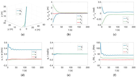
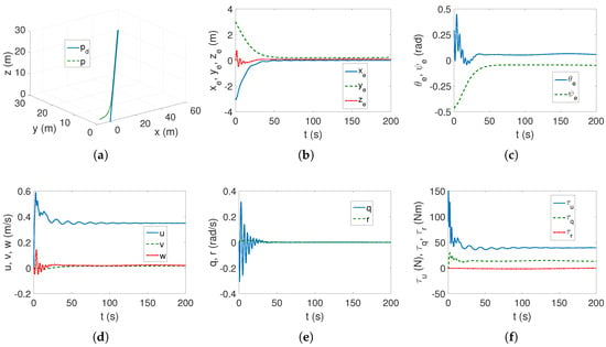
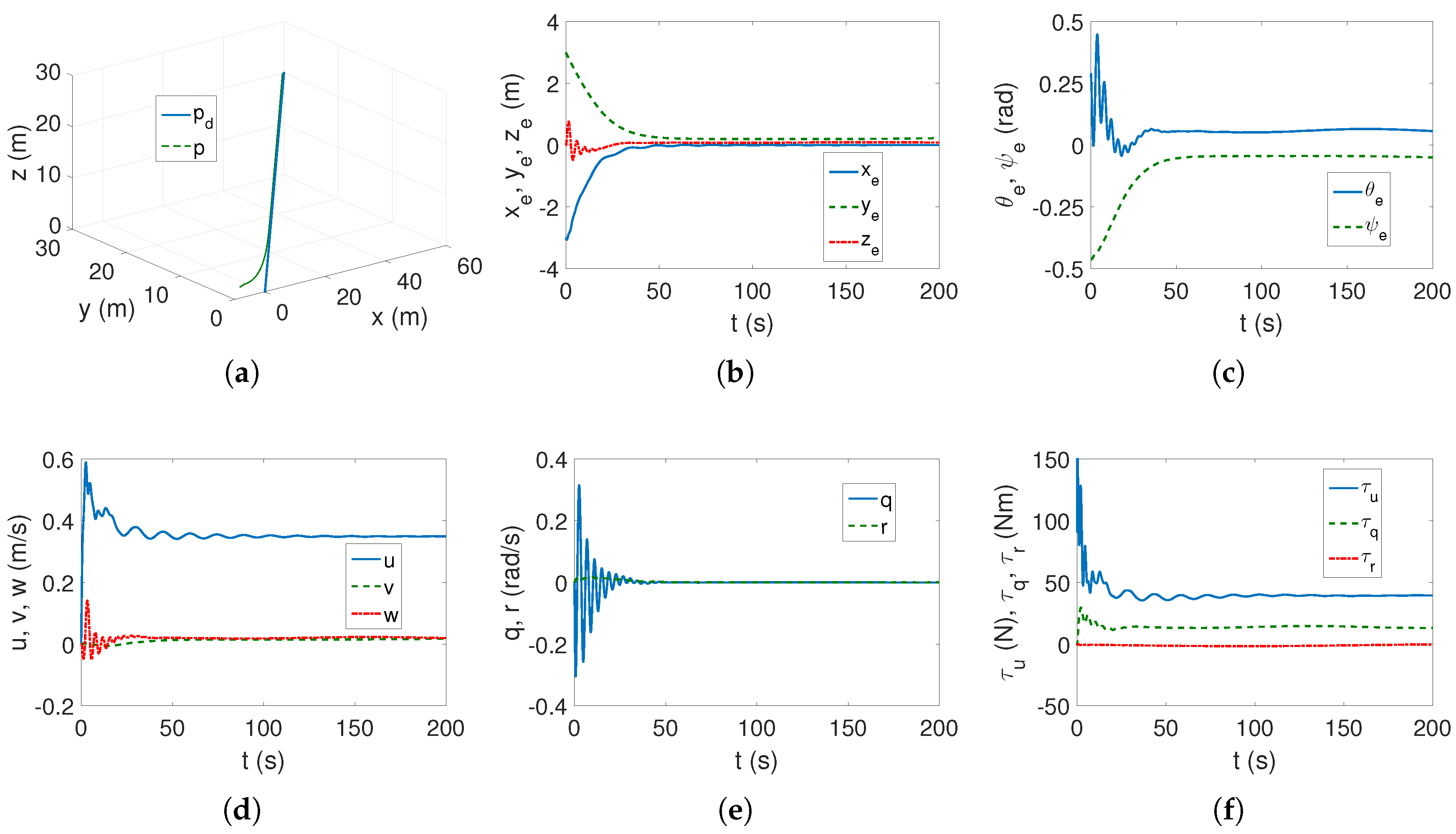
Linear trajectory (23). In Figure 2a–c, it can be observed that the linear trajectory is tracked and the linear and angular position errors have limited values (according to the theory of [39]). Linear and angular velocities, as shown in Figure 2d,e, reach constant values, although velocity v stabilizes at the last (after about 150 s). This is a result of the shift of the center of mass, but the algorithm works correctly in this situation. The force and torque values (Figure 2f) are within the limits set by the technical capabilities of the vehicle. From this, it can be concluded that the control algorithm VTBA is effective for a linear trajectory.

Figure 2. C-Ranger, VTBA algorithm, and linear trajectory: (a) desired and actual trajectory; (b) linear position errors; (c) angular position errors; (d) linear velocities; (e) angular velocities; and (f) applied force and torques.

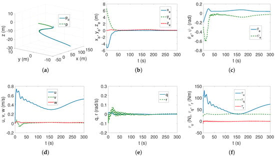
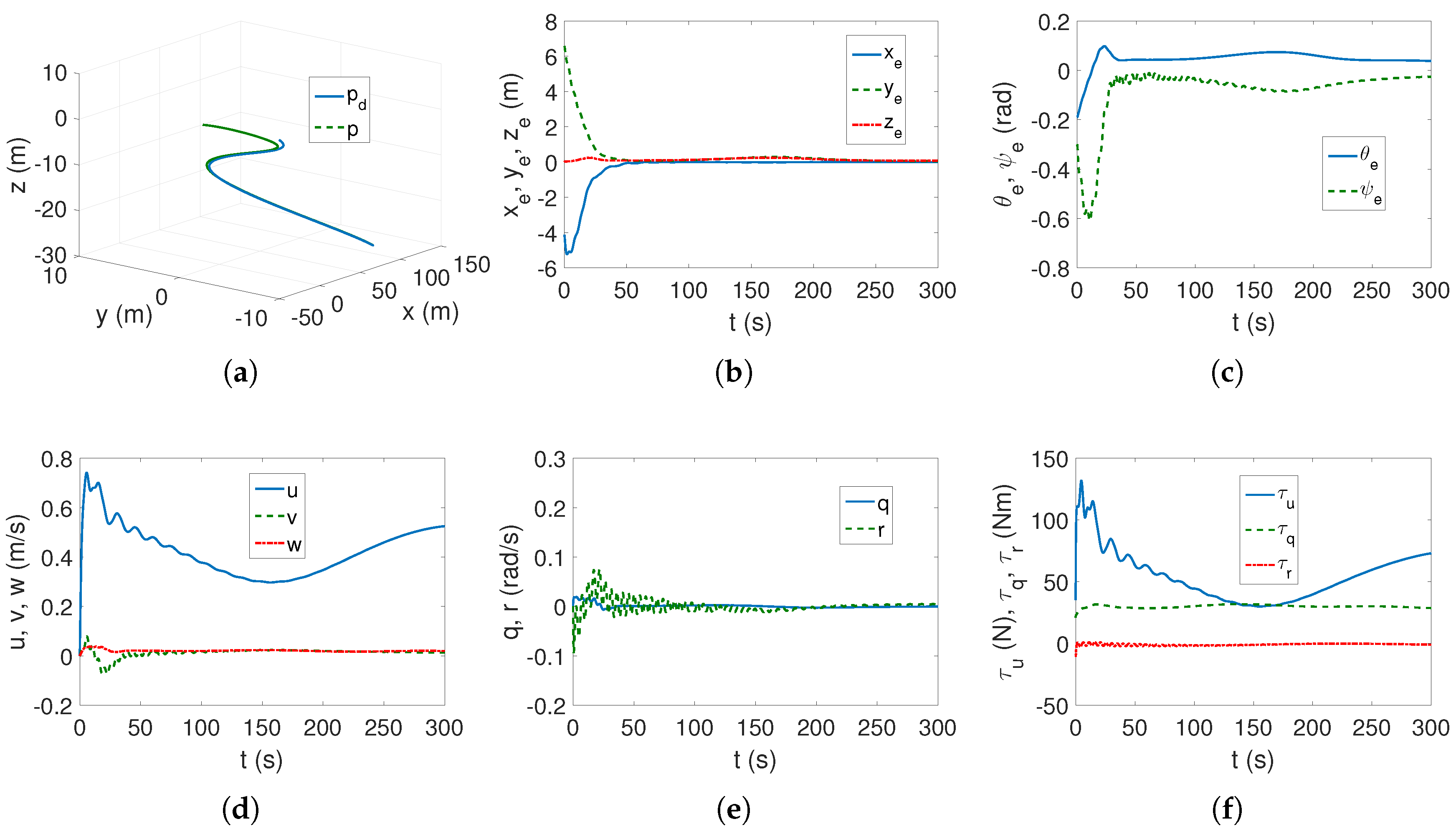
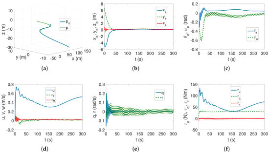
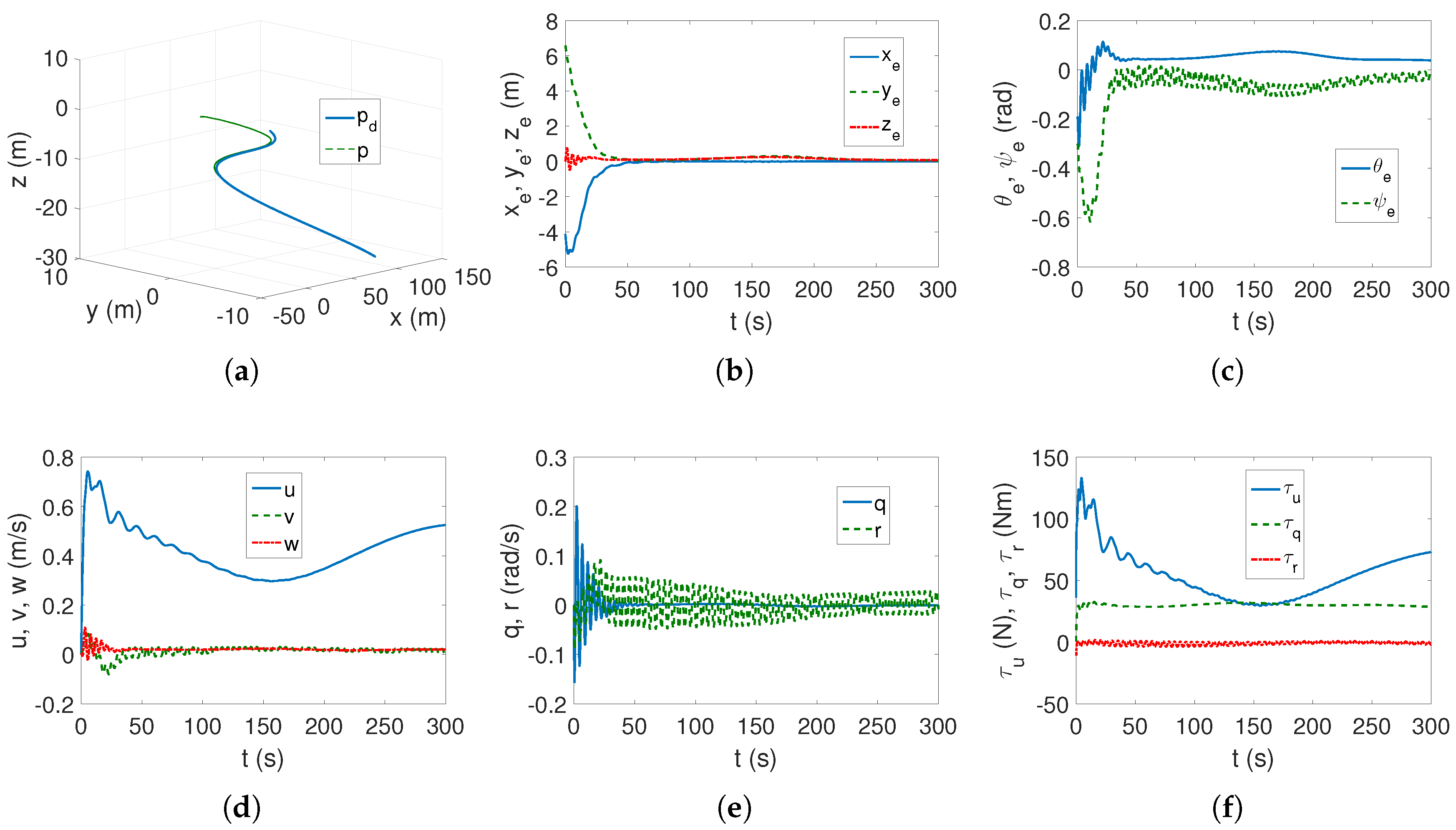
Complex trajectory (24). As can be seen in Figure 3a–c, the trajectory tracking task is performed correctly despite noticeable oscillations in the initial phase of the movement. The velocity oscillations also vanish, as can be observed in Figure 3d,e and the forward motion dominates due to velocity v. The force and moment values are also permissible, as can be observed from Figure 3f.

Figure 3. C-Ranger, VTBA algorithm, and complex trajectory: (a) desired and actual trajectory; (b) linear position errors; (c) angular position errors; (d) linear velocities; (e) angular velocities; and (f) applied force and torques.

4.3.2. Strategy RTABDIM

In this strategy, the same control parameters as those used for the VTBA algorithm were used in the tests, that is, (26) and (27), respectively. This is important because, conceptually, the RTABDIM algorithm is a simplified version of the previous dynamics model, which ignores inertial couplings resulting from the displacement of the vehicle’s center of mass. Simulation tests were performed using the author’s software based, in part, on the source code from [50] (for a three-DOF vehicle in horizontal motion and other model parameters).

Linear trajectory (23). Figure 4a,b show that the linear trajectory is correctly tracked. However, it is clear that the trajectory tracking error $z_e$ is oscillatory at the beginning of the movement, indicating that the algorithm is trying to compensate for the inaccuracies resulting from the shift in the center of mass. A similar phenomenon occurs, for the same reason, for the angular error ${\theta }_e$ (Figure 4c). Oscillations are also noticeable in the remaining Figure 4d–f. Generally, it can be concluded that, in the case of linear trajectory tracking, despite the clear motion disturbance, the algorithm achieved its task.

Figure 4. C-Ranger, RTABDIM algorithm, and linear trajectory: (a) desired and actual trajectory; (b) linear position errors; (c) angular position errors; (d) linear velocities; (e) angular velocities; and (f) applied force and torques.

Complex trajectory (24). As can be seen in Figure 5a,b, the trajectory tracking task is performed as expected. However, this is misleading because Figure 5c shows a continuous oscillatory motion of the error ${\psi }_e$. Furthermore, Figure 5d shows that the velocity v is variable instead of reaching a constant value. Figure 5e shows a variable oscillatory motion of the angular velocity r, and Figure 5f shows that the torque ${\tau }_r$ also oscillates around zero. Summarizing these observations, it cannot be assumed that the algorithm is working correctly because the vehicle will (due to inertial disturbances) perform an oscillatory motion and angular variables are particularly sensitive to shifts in the center of mass.

Figure 5. C-Ranger, RTABDIM algorithm, and complex trajectory: (a) desired and actual trajectory; (b) linear position errors; (c) angular position errors; (d) linear velocities; (e) angular velocities; and (f) applied force and torques.

4.3.3. Strategy RTCDO

The concept of a control strategy is based on generating a reference trajectory by simulating kinematic and dynamic models and assuming the initial states of positions, velocities, force, and torques. Therefore, with this method concept, it is not possible to assume a trajectory in the same way as in previous control methods.

Initial remarks. It is possible to generate a complex trajectory based on the dynamics and kinematics of the model, but not a linear trajectory. Limiting the force and torque values to realistic values caused the algorithm to stop working properly. The same effect occurred when disturbances were introduced in the form of functions defined by the operating conditions (25). The damping parameters contained only linear components due to assumptions from the original work. The introduction of center of mass shifts $x_g,z_g$ also made the trajectory tracking task impossible. The external disturbances that affect the vehicle to allow the controller to operate were determined by trial and error. Referring to function (25), they had the following values: $0.0001·f_u\left(t\right)$, $0.01·f_v\left(t\right)$, $0.01·f_w\left(t\right)$, $0.01·f_q\left(t\right)$, and $0.01·f_r\left(t\right)$.

For simulation tests, software from [51] was used, but adapted to the C-Ranger vehicle. Taking into account the above mentioned initial remarks, the following set of control parameters was selected.

$$\begin{array}{ccc}\hfill & & a_{\rho }=b_{\rho }=0.015,a_{\chi }=b_{\chi }=a_{\gamma }=b_{\gamma }=0.34,a_u=b_u=a_q=b_q=a_r=b_r=2,\hfill \\ & & T_1=T_2=T_3=0.1,a=5;b_1=b_2=20,m=1;k_0=k_1=k_2=1,\alpha =0.9,\beta =1.5.\hfill \end{array}$$

(28)

The initial states were as follows: $x\left(0\right)=y\left(0\right)=z\left(0\right)=0$ m, $\theta \left(0\right)=\psi \left(0\right)=0$ rad, $u\left(0\right)=v\left(0\right)=w\left(0\right)=0$ m/s, and $q\left(0\right)=r\left(0\right)=0$ rad/s. The reference trajectory was generated such that $x_d\left(0\right)=2$ m, $y_d\left(0\right)=-7$ m, $z_d\left(0\right)=0.3$ m, ${\theta }_d\left(0\right)={\psi }_d\left(0\right)=0$ rad, $u_d\left(0\right)=v_d\left(0\right)=w_d\left(0\right)=0$ m/s, $q_d\left(0\right)=r_d\left(0\right)=0$ rad/s, ${\tau }_{ud}=1$ N, and ${\tau }_{qd}={\tau }_{rd}=1$ Nm.

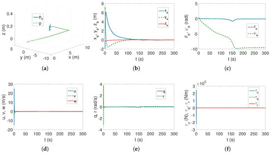
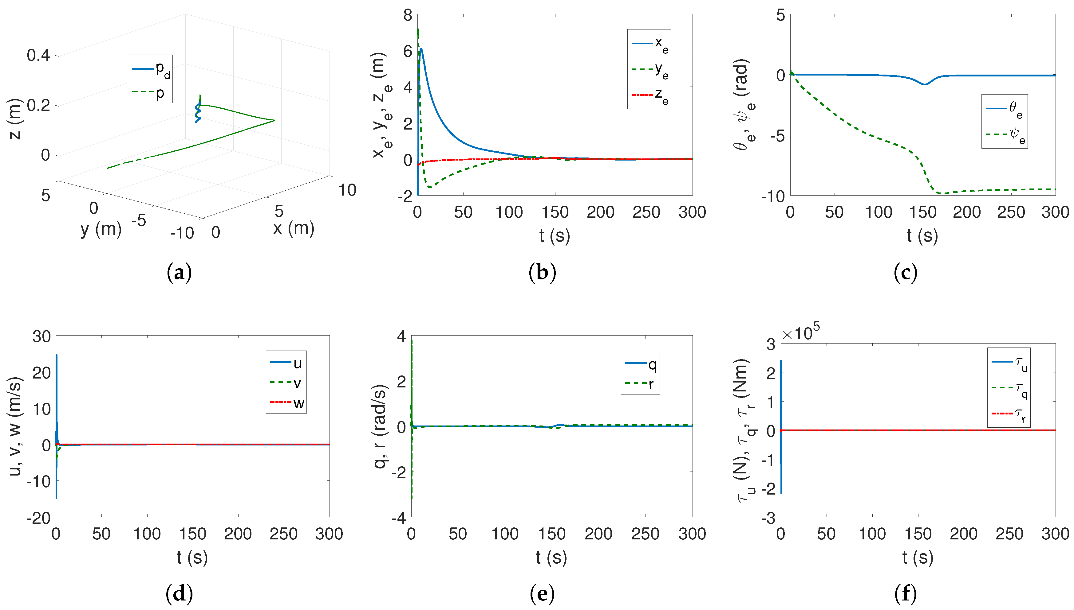
Complex trajectory. From Figure 6a,b, it can be observed that the linear trajectory is performed correctly because the desired trajectory is achieved and the position errors converge to zero. However, in Figure 6c, it can be seen that the error of the rotation variable ${\psi }_e$ is almost 10 rad, which means that the vehicle will rotate three times around the vertical axis during its motion. The initial linear and angular velocities have values that are practically impossible to achieve, as shown in Figure 6d,e. The force value ${\tau }_u$ is also unrealistic for the engines mounted on the tested vehicle as shown in Figure 6f.

Figure 6. C-Ranger, RTCDO algorithm, and complex trajectory: (a) desired and actual trajectory; (b) linear position errors; (c) angular position errors; (d) linear velocities; (e) angular velocities; and (f) applied force and torques.

Comment. Although ref. [16] presented results confirming the effectiveness of the control strategy, in the research presented here, the proposed approach proved to be useless. This discrepancy between the examples demonstrates that a vehicle model can be selected to meet the trajectory tracking expectations. Unfortunately, under simulation conditions close to reality (another controller operating condition or another vehicle model used in marine research), the strategy may not yield acceptable results.

4.3.4. Strategy IGTCSH

This control strategy allows for tracking a linear trajectory. Therefore, the tests used a linear trajectory defined according to the conditions given in [6].

Initial remarks. In preliminary tests, it turned out that it is possible to include the shift of the center of mass $x_g,z_g$ in the dynamics equations. Since the control algorithm ran quickly, the runtime was reduced to 50 s. Two cases were also considered as follows: Case 1 (without control signal constraints) and Case 2 (with these signals restricted for the C-Ranger vehicle). Since the algorithm turned out to be sensitive to the sampling time, $\Delta t=0.02$ s was assumed.

For simulation tests, software from [52] was used, but adapted to the C-Ranger vehicle. The set of control parameters established as a result of the test trials is as follows.

$$\begin{array}{ccc}\hfill & & k_1=k_2=k_3=2.5,k_4=k_5=10,k_6=k_7=k_8=1.0,k_i=0.05,i=u,\alpha ,\beta ,q,r.\hfill \end{array}$$

(29)

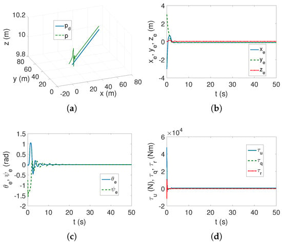
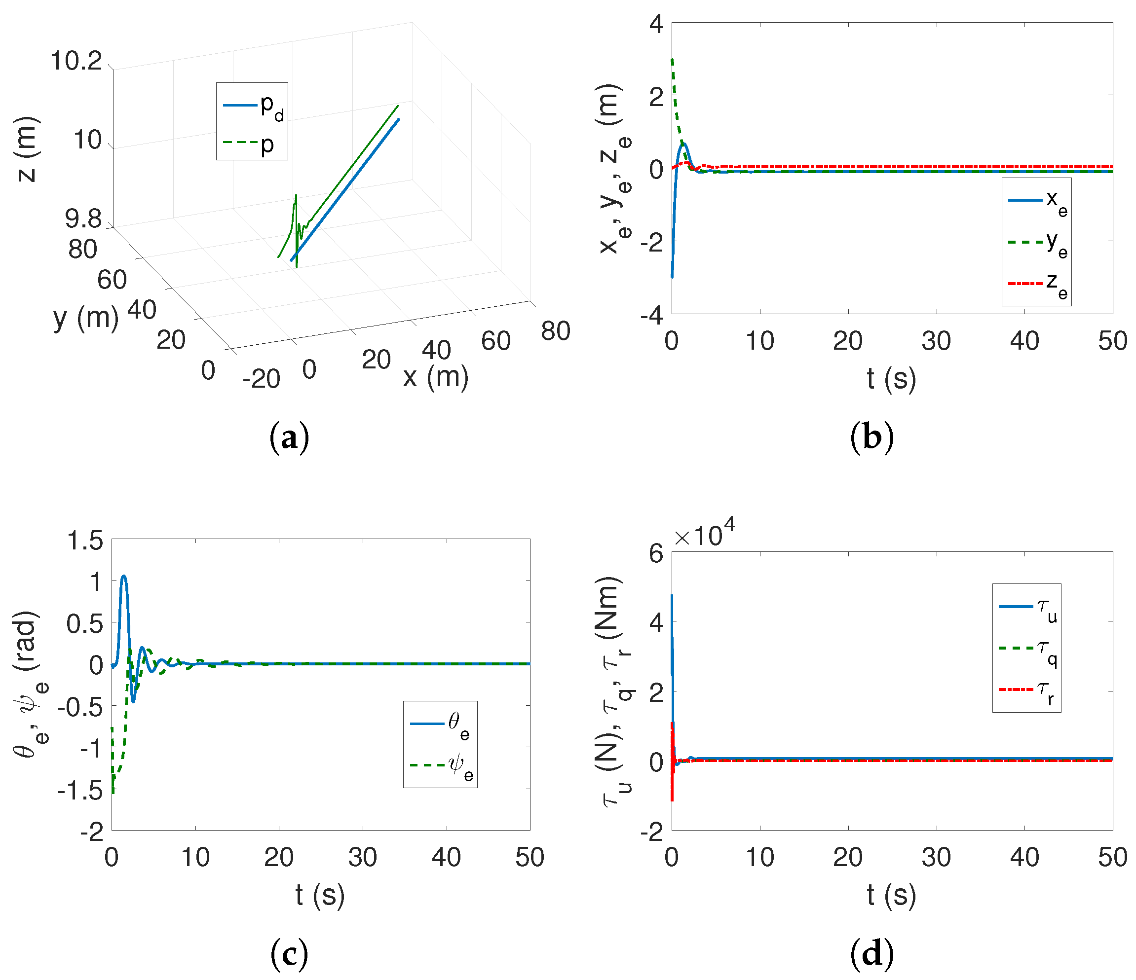
If the values of force and torque are not limited, then, as can be seen in Figure 7a,b, the trajectory is tracked with certain errors $x_e,y_e$ with constant values. Figure 7c shows that the angular errors approach zero but are large at the beginning of the movement. However, as can be seen in Figure 7d, when the vehicle begins to move, the force and torque values are so high that they cannot be achieved in the test vehicle.

Figure 7. C-Ranger, IGTCSH algorithm, and linear trajectory Case 1: (a) desired and actual trajectory; (b) linear position errors; (c) angular position errors; and (d) applied force and torques.

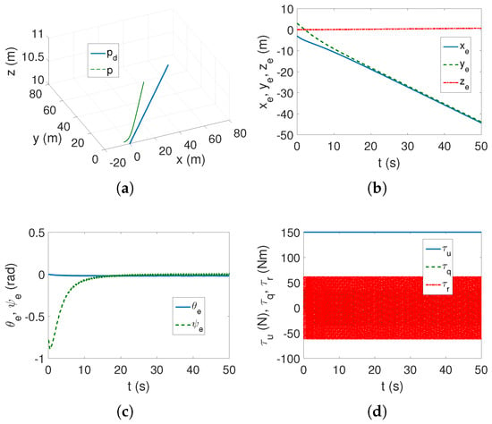
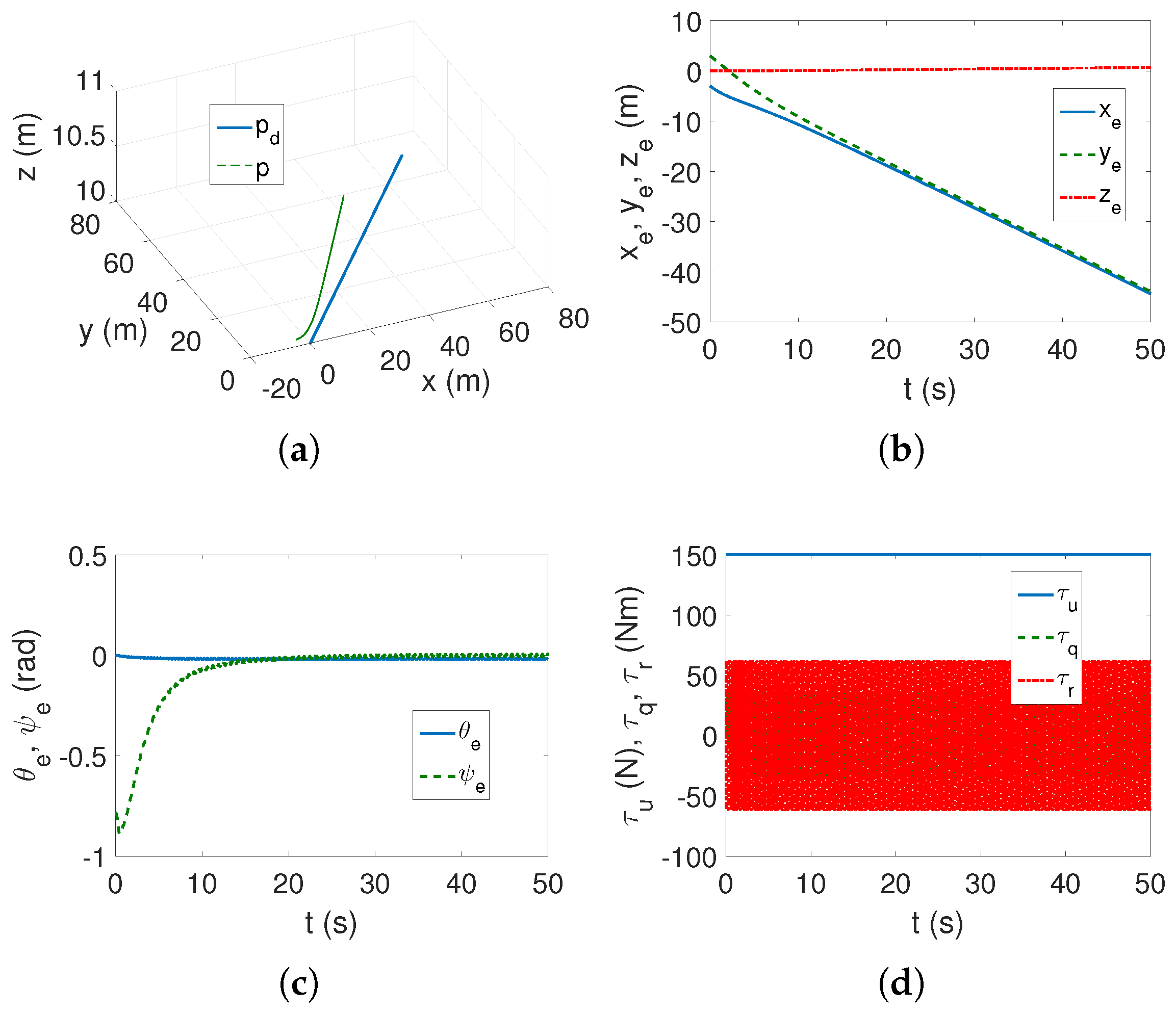
Due to unrealistic results for Case 1, Case 2 was investigated, in which the achievable force and torque values are limited. As can be seen in Figure 8a,b, the algorithm does not track the trajectory. The angular errors tend to be very small (Figure 8c), but the force and torque values in Figure 8d indicate that the controller is operating at maximum values, which would certainly lead to vehicle destruction or at least to controller termination.

Figure 8. C-Ranger, IGTCSH algorithm, and linear trajectory Case 2: (a) desired and actual trajectory; (b) linear position errors; (c) angular position errors; and (d) applied force and torques.

Comment. In simulation tests, it turned out that this type of control scheme is not suitable for the linear trajectory tracking task, although its effectiveness was indicated in [6].

4.3.5. Strategy TABBASMC

For this control strategy, all the test assumptions stated earlier in this section were met. For simulation tests, software from [52] was used, but adapted to the C-Ranger vehicle.

The numerical tests were performed using the following sets of control parameters defined in [15]:

$$\begin{array}{ccc}\hfill & & \mathrm{Linear} \mathrm{trajectory}{b}_1=b_2=b_3=10,k=1,\delta =0.1,{\zeta }_1={\zeta }_2={\zeta }_3=300,\hfill \end{array}$$

(30)

$$\begin{array}{ccc}\hfill & & \mathrm{Complex} \mathrm{trajectory}{b}_1=b_2=b_3=10,k=1,\delta =0.1,{\zeta }_1={\zeta }_2={\zeta }_3=1500.\hfill \end{array}$$

(31)

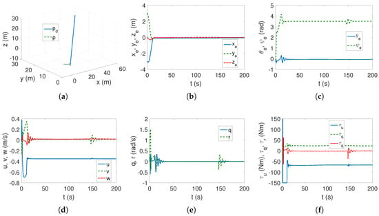
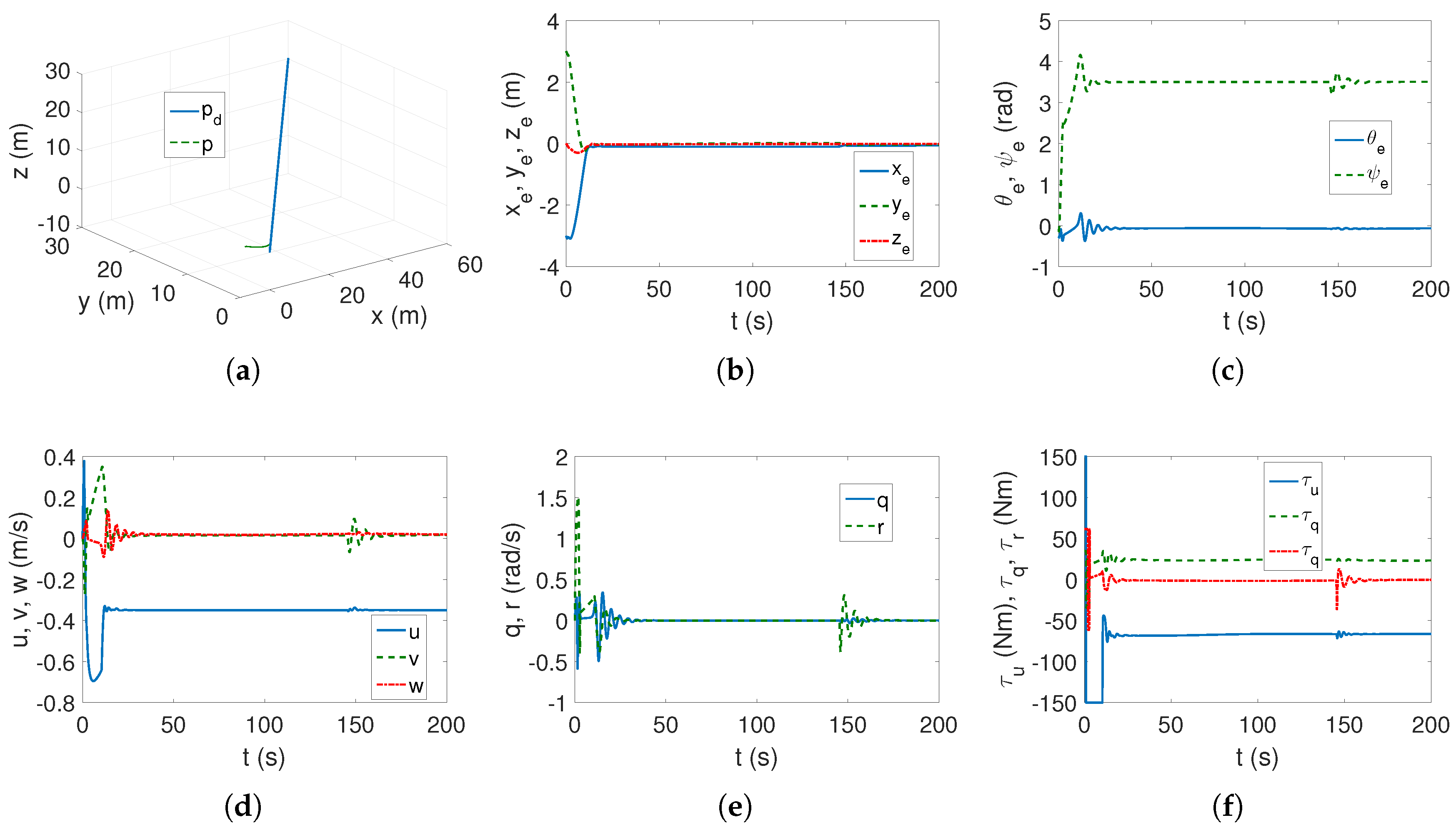
Linear trajectory (23). The linear trajectory is tracked correctly, as shown in Figure 9a, and the linear position errors are within acceptable values, as can be seen in Figure 9b. However, there is a problem with the angular position errors, as can be observed in Figure 9c. Instead of approaching zero, the ${\psi }_e$ error reaches a value of about 3.5 rad after about 20 s. Therefore, in a short time, the vehicle completes about half a rotation around the vertical axis and remains in that position. This means that there is no control over the $\psi$ variable. Figure 9d–f show that the values of linear speed, angular speed, and torque are acceptable for the C-Ranger vehicle. In Figure 9d, it appears that the vehicle moves backward instead of forward (the velocity u has negative values). However, some concerns arise regarding changes of these variables that occur after approximately 150 s of motion (the time after which this phenomenon occurs depends on the set of control parameters). This is concerning because the tracked trajectory is linear, and sudden changes in these values once they are established should not cause such a phenomenon.

Figure 9. C-Ranger, TABBASMC algorithm, and linear trajectory: (a) desired and actual trajectory; (b) linear position errors; (c) angular position errors; (d) linear velocities; (e) angular velocities; and (f) applied force and torques.

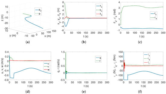
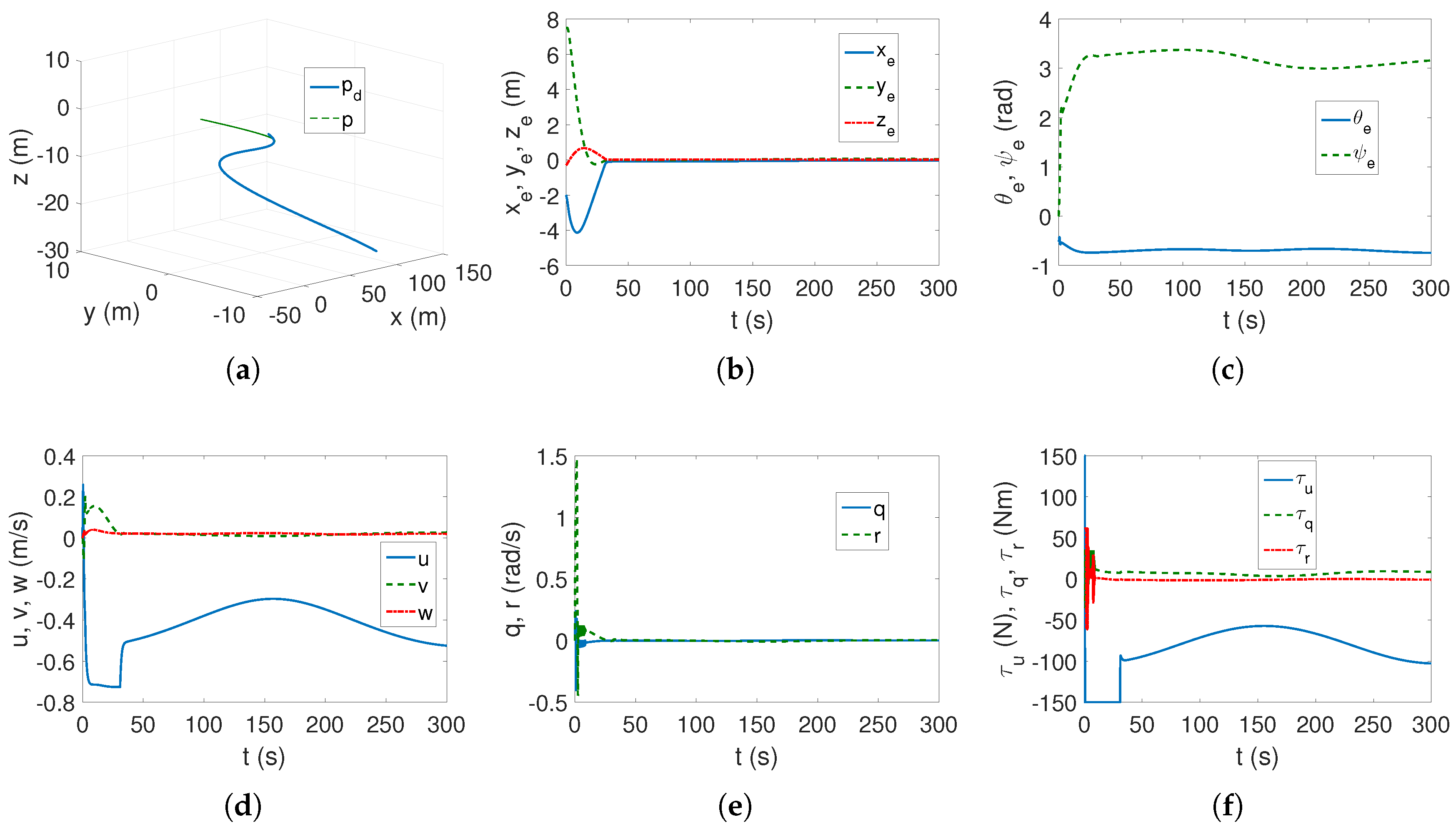
Complex trajectory (24). Based on Figure 10a,b, it can be concluded that the complex trajectory tracking task is performed correctly. However, Figure 10c shows that errors ${\theta }_e,{\psi }_e$ are not controlled. Therefore, the control scheme is not fully effective. Figure 10d–f show linear and angular velocities, forces, and torques, respectively, and their values are achievable for the C-Ranger vehicle. However, in Figure 10d, it appears that the vehicle moves backward instead of forward (the velocity u has negative values).

Figure 10. C-Ranger, TABBASMC algorithm, and complex trajectory: (a) desired and actual trajectory; (b) linear position errors; (c) angular position errors; (d) linear velocities; (e) angular velocities; and (f) applied force and torques.

Comment. The control strategy proposed in [15] proved to be only partially effective. Although linear position tracking can be achieved, angular position tracking cannot be controlled. Moreover, the results depend on the effectiveness of the linear position error reduction. This means that the vehicle will rotate around one or two axes. In the reference work, angular position errors were not shown.

4.3.6. Summary of Numerical Results

To obtain a quantitative comparison, the values of the indexes selected for the evaluation of the effectiveness of each control strategy were calculated.

The results based on the quality indexes obtained with linear trajectory tracking are given in Table 2. In this table, the following abbreviations are used: F means ‘failed’, N/A means ‘not applicable’.

Table 2. Performance for C-Ranger for linear trajectory.

Index	VTBA	RTABDIM	RTCDO	IGTCSH	TABBASMC
MIA $x_e$	0.1797	0.1797	N/A	F	0.2020
MIA $y_e$	0.4168	0.4173	N/A	F	0.0879
MIA $z_e$	0.0809	0.0914	N/A	F	0.0285
MIAE $e_L$	0.6774	0.6884	N/A	F	0.3184
RMS $\left|\right|e_L\left|\right|$	0.8841	0.8877	N/A	F	0.6666
MIA ${\theta }_e$	0.0593	0.0615	N/A	F	0.0770
MIA ${\psi }_e$	0.0840	0.0841	N/A	F	3.4570
MIAE $e_A$	0.1434	0.1456	N/A	F	3.5339
RMS $\left|\right|e_A\left|\right|$	0.1434	0.1471	N/A	F	3.4727
MIAC $\tau$	43.461	43.503	N/A	F	75.470

The quantitative results confirmed that the VTBA scheme outperformed the RTABDIM algorithm (lower numerical values). This suggests that if the center of mass shifts are not included in the control equations, the trajectory tracking accuracy will be poorer even for small shifts (here, 1 to 1.5 cm). In the TBBASMC control strategy, the linear position error values were lower than those of VTBA and RTABDIM, indicating that the algorithm performed very well when the center of mass was shifted. However, the angular position errors are very large. This implies that these errors cannot be controlled and as a result, the vehicle rotates when the algorithm performs the trajectory tracking task. The energy consumption measured by the control signal values is much higher when using the TBBASMC algorithm than when using the VTBA and RTABDIM algorithms. The RTCDO algorithm is not applicable when the trajectory is linear, while the IGTCSH algorithm failed.

Taking into account the results in Table 3, it can be observed that the VTBA strategy is also more effective than the RTABDIM strategy, as the former yielded lower index values. The TABBASMC algorithm, on the other hand, proved to be very accurate again, but only when tracking linear positions, as the angular positions were again uncontrolled and resulted from the vehicle’s motion. In turn, the RTCDO algorithm failed in the case of a complex trajectory and the IGTCSH algorithm is not applicable.

Table 3. Performance for C-Ranger for complex trajectory.

Index	VTBA	RTABDIM	RTCDO	IGTCSH	TABBASMC
MIA $x_e$	0.2997	0.3000	F	N/A	0.3424
MIA $y_e$	0.3968	0.3971	F	N/A	0.2465
MIA $z_e$	0.1391	0.1458	F	N/A	0.0595
MIAE $e_L$	0.8356	0.8430	F	N/A	0.6483
RMS $\left|\right|e_L\left|\right|$	1.4510	1.4540	F	N/A	1.4351
MIA ${\theta }_e$	0.0543	0.0545	F	N/A	0.6903
MIA ${\psi }_e$	0.0813	0.0819	F	N/A	3.1381
MIAE $e_A$	0.1356	0.1364	F	N/A	3.8284
RMS $\left|\right|e_A\left|\right|$	0.1529	0.1550	F	N/A	3.2251
MIAC $\tau$	63.262	63.289	F	N/A	85.759

4.3.7. Discussion of Results

Five control strategies were tested; the first of them were intended for the model with shifted center of the mass in relation to the geometric center; in the other four, these centers should be at the same point. In order to make the results more real, the model representing the underwater vehicle used in sea tests was assumed, and the drive limitations were due to real possibilities defined by the technical data.

From the research performed in the defined work conditions, observations can be made as follows:

• VTBA strategy. This control scheme proved useful for the tracking of complex and linear trajectories. All position errors and other quantities were within acceptable limits. However, it should be noted that this algorithm is designed for this type of control, namely if the center of mass displacement occurs.
• RTABDIM strategy. The algorithm designed for the vehicle model with inertial coupling omitted for small center of mass shifts (1 to 1.5 cm) performed the trajectory tracking task in both tested cases. However, oscillations occurred in the first phase of the movement. Furthermore, for the complex trajectory, these oscillations did not disappear for angular position errors. This means that the vehicle constantly vibrated around the z axis and its velocity also varied oscillatory. It can therefore be concluded that while tracking the linear trajectory is effective, the complex trajectory is not tracked correctly (due to the vehicle rotation around the axis).
• RTCDO strategy. This control strategy proved completely unsuitable for the trajectory tracking task. Even assuming a complex trajectory (as in the reference work), no acceptable results could be obtained for the C-Ranger vehicle model (even without introducing a center of mass shift).
• IGTCSH strategy. When force and torque limits were ignored, the algorithm worked for a linear trajectory, but at the beginning of the movement, the angular position errors were large, and the force and torque values were impossible to achieve for the C-Ranger vehicle. After introducing the force and torque limits, the algorithm completely failed. Moreover, a complex trajectory cannot be tracked for this algorithm.
• TABBASMC strategy. For this control scheme, the linear and complex trajectory tracking errors were even smaller than those of the VTBA and RTABDIM algorithms, but only for linear positions. This indicates that the TABBASMC strategy works correctly for these quantities. Unfortunately, angular position errors were not accounted for in the input signals and depended on the algorithm’s operation, leading to large errors and vehicle rotation around the vertical axis. Instead of moving forward, the vehicle moved backward, which may not be a problem, but is also unnatural for commonly used controllers. In addition, the energy consumption measured by the input signal values was higher than those of the two aforementioned algorithms. Therefore, it can be concluded that the TABBASMC strategy requires further improvement to also reduce angular position errors. In summary of the test results, this controller did not achieve satisfactory performance.

Remarks on the tests.

• The simulation tests were performed for a C-Ranger vehicle model, which is used in marine research and therefore can be assumed to be a model of a real vehicle.
• To compare the performance in the event of a shift in the vehicle’s center of mass, several control schemes were selected, the effectiveness of which was confirmed in the literature on marine vehicle control.
• The simulation tests conducted revealed two serious problems. The first is that even if the control strategy proved effective in the reference work, changing a vehicle model used in marine research or assuming different operating conditions may not yield acceptable results at all. The second problem is related to situations where a small displacement of the center of mass occurs (e.g., 1 to 1.5 cm). This may lead to a decrease in the performance of the control algorithm or even the inability to track the trajectory.

Remark. The problem of control effectiveness when the center of the mass is shifted was considered in [39] and then in [23,53]. However, this issue has still been omitted, e.g., [10,13,20,24], which means that it is not known how the control scheme will work when this situation occurs. This may result in the fact that the control may prove to be useless from a practical point of view.

Summary. A summary of the effectiveness of the control algorithms considered is provided in Table 4. Explanation of the symbols used follows: P.E. Linear—linear position error, P.E. Angular—angular position error, Error $x_e$, Error $z_e$ error in underactuated directions, MCSR—mass center shift robustness, CIV—control input value, ‘+’ means acceptable results, ‘*’ means sometimes acceptable results (longer or permanently oscillatory motion), ‘–’ means unacceptable results, ‘++’ means better results (smaller values of errors and control signals).

Table 4. Effectiveness of control schemes.

	VTBA	RTABDIM	RTCDO	IGTCSH	TABBASMC
P.E. Linear	+	+	–	–	++
Error $x_e$	++	++	–	–	+
Error $z_e$	+	+ *	–	–	++
P.E. Angular	++	+ *	–	–	–
MCSR	++	+ *	–	–	–
CIV	++	++	–	–	+

The observations concern the main problem, namely the robustness of each control strategy to small displacements of the center of mass. The VTBA control scheme, dedicated to situations in which the center of mass may be shifted, always produced acceptable results in the tests performed. In turn, the RTABDIM algorithm, which did not take this shift into account, was less effective and did not necessarily lead to acceptable results. However, the RTCDO and IGTCSH strategies proved to be unsuitable in the situation considered. The last strategy tested yielded very good or acceptable results, but only for linear position errors. Unfortunately, because of the lack of control of the angular errors, it cannot be considered an effective trajectory tracking method.

4.3.8. Notes on Model Uncertainty and Complex Dynamics

The issue of model complexity and the uncertainty of its parameters primarily concerns the description when the six-DOF dynamics equations are used. One can recall works that present modern control schemes based on such a model, e.g., [3,54,55,56,57,58,59]. Since in this work control strategies based on a five-DOF model were tested, the problem of its complexity is not considered. For a model reduced to five DOF, the inertia matrix is generally assumed to be diagonal. This simplifies the dynamics model. Only occasionally is the problem of model parameter uncertainty considered, as in [7,10,17,27,60,61]. The design of a control algorithm based on a symmetric inertia matrix was proposed in [39].

5. Conclusions

This work compared five control schemes based on the five-DOF model in terms of their effectiveness in the implementation of the trajectory tracking task. The problem is important because the model with a diagonal inertia matrix is usually applied for designing control algorithms, which means that dynamic couplings between variables, even if they actually exist, are omitted without a deeper analysis regarding the consequences of such an assumption.

The tests show that the algorithm, which is based on the model taking into account the displacement of the center of the mass, is effective when this situation occurs. However, if the model is simplified (which means a diagonal inertia matrix), only one of the algorithms produced almost-acceptable results. Other control strategies have failed or have only partially led to acceptable results. Therefore, it can be concluded that algorithms that use the simplified five-DOF model should be verified to move the center of mass to check their effectiveness. If this is not verified, and simulation tests were not confirmed by a real experiment, then such algorithms have a primarily mathematical value but not necessarily a value from a technical point of view. It can also be concluded that the issue of verifying the effectiveness of the control scheme is important and should be taken into account when designing new control methods.

Future work should address two issues: first, designing control algorithms based on a dynamics model with a symmetric inertia matrix. Second, disturbance models that would represent dynamic elements lost during modelreduction.

References

- Fossen, T.I. Guidance and Control of Ocean Vehicles; John Wiley and Sons: Chichester, UK, 1994. [Google Scholar]
- Do, K.D.; Pan, J. Control of Ships and Underwater Vehicles; Springer: London, UK, 2009. [Google Scholar]
- Hu, Y.; Li, B.; Jiang, B.; Han, J.; Wen, C.-Y. Disturbance Observer-Based Model Predictive Control for an Unmanned Underwater Vehicle. J. Mar. Sci. Eng. 2024, 12, 94. [Google Scholar] [CrossRef] [Scilit]
- Thanh, P.N.N.; Thuyen, N.A.; Anh, H.P.H. Adaptive fuzzy 3-D trajectory tracking control for autonomous underwater vehicle (AUV) using modified integral barrier lyapunov function. Ocean Eng. 2023, 283, 115027. [Google Scholar] [CrossRef] [Scilit]
- Xu, R.; Tang, G.; Xie, D.; Han, L.; Huang, H. Neural network for 3D trajectory tracking control of a CMG-actuated underwater vehicle with input saturation. ISA Trans. 2022, 123, 152–167. [Google Scholar] [CrossRef] [Scilit] [PubMed]
- Yan, Z.; Wang, M.; Xu, J. Integrated guidance and control strategy for homing of unmanned underwater vehicles. J. Frankl. Inst. 2019, 356, 3831–3848. [Google Scholar] [CrossRef] [Scilit]
- Jiang, Y.; Guo, C.; Yu, H. Robust trajectory tracking control for an underactuated autonomous underwater vehicle based on bioinspired neurodynamics. Int. J. Adv. Robot. Syst. 2018, 15, 1729881418806745. [Google Scholar] [CrossRef] [Scilit]
- Zhou, J.; Ye, D.; Zhao, J.; He, D. Three-dimensional trajectory tracking for underactuated AUVs with bio-inspired velocity regulation. Int. J. Nav. Archit. Ocean Eng. 2018, 10, 282–293. [Google Scholar] [CrossRef] [Scilit]
- Yu, H.; Guo, C.; Shen, Z.; Yan, Z. Output Feedback Spatial Trajectory Tracking Control of Underactuated Unmanned Undersea Vehicles. IEEE Access 2020, 8, 42924–42936. [Google Scholar] [CrossRef] [Scilit]
- Liu, J.; Du, J.; Wang, J. Predefined-time asymptotic control for the 3-D trajectory tracking of underactuated AUVs under asymmetric input saturations. Ocean Eng. 2025, 332, 121415. [Google Scholar] [CrossRef] [Scilit]
- Xie, T.; Li, Y.; Jiang, Y.; An, L.; Wu, H. Backstepping active disturbance rejection control for trajectory tracking of underactuated autonomous underwater vehicles with position error constraint. Int. J. Adv. Robot. Syst. 2020, 17, 1729881420909633. [Google Scholar] [CrossRef] [Scilit]
- Chen, H.; Tang, G.; Wang, S.; Guo, W.; Huang, H. Adaptive fixed-time backstepping control for three-dimensional trajectory tracking of underactuated autonomous underwater vehicles. Ocean Eng. 2023, 275, 114109. [Google Scholar] [CrossRef] [Scilit]
- Qian, F.; Zheng, Y.; Wang, A.; Cai, J. Event-Triggered Adaptive Backstepping Control of Underactuated AUVs with Input Saturation. Electronics 2025, 14, 1839. [Google Scholar] [CrossRef] [Scilit]
- Chen, Q.; Yuan, J.; Dong, Z.; Chai, Z.; Wan, L. Enhanced Control Strategies for Underactuated AUVs Using Backstepping Integral Sliding Mode Techniques for Ocean Current Challenges. J. Mar. Sci. Eng. 2024, 12, 2201. [Google Scholar] [CrossRef] [Scilit]
- Guo, Q.; Li, Y.; Liu, H.; Xiang, J. An Underactuated AUV Tracking Algorithm Based on Backstepping Adaptive Sliding Mode Control. In Proceedings of the 2020 Chinese Automation Congress (CAC), Shanghai, China, 6–8 November 2020; pp. 3765–3770. [Google Scholar]
- An, S.; Wang, L.; He, Y. Robust fixed-time tracking control for underactuated AUVs based on fixed-time disturbance observer. Ocean Eng. 2022, 266, 112567. [Google Scholar] [CrossRef] [Scilit]
- Liu, H.; Zhuo, J.; Tian, X.; Mai, Q. Finite-time self-structuring neural network trajectory tracking control of underactuated autonomous underwater vehicles. Ocean Eng. 2023, 268, 113450. [Google Scholar] [CrossRef] [Scilit]
- Cao, J.; Sun, Y.; Zhang, G.; Jiao, W.; Wang, X.; Liu, Z. Target tracking control of underactuated autonomous underwater vehicle based on adaptive nonsingular terminal sliding mode control. Int. J. Adv. Robot. Syst. 2020, 17, 1729881420919941. [Google Scholar] [CrossRef] [Scilit]
- Liu, J.; Du, J. Composite learning tracking control for underactuated autonomous underwater vehicle with unknown dynamics and disturbances in three-dimension space. Appl. Ocean Res. 2021, 112, 102686. [Google Scholar] [CrossRef] [Scilit]
- Guo, L.; Zhou, R.; Guo, Q.; Ma, L.; Hu, C.; Luo, J. Spatial Trajectory Tracking of Underactuated Autonomous Underwater Vehicles by Model–Data-Driven Learning Adaptive Robust Control. J. Mar. Sci. Eng. 2025, 13, 1151. [Google Scholar] [CrossRef] [Scilit]
- Zhang, X.; Jiang, K. Backstepping-based adaptive control of underactuated AUV subject to unknown dynamics and zero tracking errors. Ocean Eng. 2024, 302, 117640. [Google Scholar] [CrossRef] [Scilit]
- Xu, J.; Cui, Y.; Yan, Z.; Huang, F.; Du, X.; Wu, D. Event-triggered adaptive target tracking control for an underactuated autonomous underwater vehicle with actuator faults. J. Frankl. Inst. 2023, 360, 2867–2892. [Google Scholar] [CrossRef] [Scilit]
- Yang, G.; Liu, W.; Li, L.; Xu, J.; Guo, L.; Zhang, K. Optimized Trajectory Tracking for ROVs Using DNN + ENMPC Strategy. J. Mar. Sci. Eng. 2024, 12, 1827. [Google Scholar] [CrossRef] [Scilit]
- Wen, J.; Zhang, J.; Yu, G. Predefined-Time Three-Dimensional Trajectory Tracking Control for Underactuated Autonomous Underwater Vehicles. Appl. Sci. 2025, 15, 1698. [Google Scholar] [CrossRef] [Scilit]
- Gong, H.; Er, M.J.; Liu, Y. Robust adaptive optimal trajectory tracking control for underactuated AUVs with position and velocity constraints in three-dimensional space. Int. J. Robust Nonlinear Control 2024, 34, 10704–10730. [Google Scholar] [CrossRef] [Scilit]
- Su, Z.; Huang, B.; Miao, J.; Lin, X. Segmented hybrid event-triggered control for underactuated autonomous underwater vehicles with an asymmetrical prescribed performance constraint. Int. J. Robust Nonlinear Control 2024, 34, 7722–7745. [Google Scholar] [CrossRef] [Scilit]
- Liu, H.; Feng, Z.; Tian, X.; Mai, Q. Robust Fixed-Time 3D Trajectory Tracking Control for Underactuated AUVs Based on a Fixed-Time SSNN Disturbance Observer. IEEE Access 2024, 12, 73652–73666. [Google Scholar] [CrossRef] [Scilit]
- Ma, D.; Chen, X.; Ma, H.; Zheng, H.; Qu, F. Neural Network Model-Based Reinforcement Learning Control for AUV 3-D Path Following. IEEE Trans. Intell. Veh. 2024, 9, 893–904. [Google Scholar] [CrossRef] [Scilit]
- Wang, T.; Peng, X.; Wang, T.; Liu, T.; Xu, D. Automated design of action advising trigger conditions for multiagent reinforcement learning: A genetic programming-based approach. Swarm Evol. Comput. 2024, 85, 101475. [Google Scholar] [CrossRef] [Scilit]
- Zhang, W.; Wu, W.; Li, Z.; Du, X.; Yan, Z. Three-Dimensional Trajectory Tracking of AUV Based on Nonsingular Terminal Sliding Mode and Active Disturbance Rejection Decoupling Control. J. Mar. Sci. Eng. 2023, 11, 959. [Google Scholar] [CrossRef] [Scilit]
- Zhang, Z.; Lin, M.; Li, D.; Lin, R. Gaze-Assisted Prescribed Performance Controller for AUV Trajectory Tracking in Time-Varying Currents. J. Mar. Sci. Eng. 2024, 12, 1643. [Google Scholar] [CrossRef] [Scilit]
- Li, J.; Du, J.; Zhu, G.; Lewis, F.L. Simple adaptive trajectory tracking control of underactuated autonomous underwater vehicles under LOS range and angle constraints. IET Control Theory Appl. 2020, 14, 283–290. [Google Scholar] [CrossRef] [Scilit]
- Yu, H.; Guo, C.; Yan, Z. Globally finite-time stable three-dimensional trajectory-tracking control of underactuated UUVs. Ocean Eng. 2019, 189, 106329. [Google Scholar] [CrossRef] [Scilit]
- Zhou, J.; Zhao, X.; Feng, Z.; Wu, D. Trajectory tracking sliding mode control for underactuated autonomous underwater vehicles with time delays. Int. J. Adv. Robot. Syst. 2020, 17, 1729881420916276. [Google Scholar] [CrossRef] [Scilit]
- Refsnes, J.E.; Sorensen, A.J.; Pettersen, K.Y. Model-Based Output Feedback Control of Slender-Body Underactuated AUVs: Theory and Experiments. IEEE Trans. Control Syst. Technol. 2008, 16, 930–946. [Google Scholar] [CrossRef] [Scilit]
- Wiig, M.S.; Pettersen, K.Y.; Krogstad, T.R. A 3D reactive collision avoidance algorithm for underactuated underwater vehicles. J. Field Robot. 2020, 37, 1094–1122. [Google Scholar] [CrossRef] [Scilit]
- Cho, G.R.; Kang, H.; Kim, M.G.; Lee, M.J.; Li, J.H.; Kim, H.; Lee, H.; Lee, G. An Experimental Study on Trajectory Tracking Control of Torpedo-like AUVs Using Coupled Error Dynamics. J. Mar. Sci. Eng. 2023, 11, 1334. [Google Scholar] [CrossRef] [Scilit]
- Gong, H.; Er, M.J.; Liu, Y. Fuzzy Optimal Fault-Tolerant Trajectory Tracking Control of Underactuated AUVs With Prescribed Performance in 3-D Space. IEEE Trans. Syst. Man Cybern. Syst. 2025, 55, 170–182. [Google Scholar] [CrossRef] [Scilit]
- Herman, P. Nonlinear Trajectory Tracking Controller for Underwater Vehicles with Shifted Center of Mass Model. Appl. Sci. 2024, 14, 5376. [Google Scholar] [CrossRef] [Scilit]
- Kim, M.; Joe, H.; Kim, J.; Yu, S. Integral sliding mode controller for precise manoeuvring of autonomous underwater vehicle in the presence of unknown environmental disturbances. Int. J. Control 2015, 88, 2055–2065. [Google Scholar] [CrossRef] [Scilit]
- Kim, J.; Joe, H.; Yu, S.-C.; Lee, J.S.; Kim, M. Time-Delay Controller Design for Position Control of Autonomous Underwater Vehicle Under Disturbances. IEEE Trans. Ind. Electron. 2016, 63, 1052–1061. [Google Scholar] [CrossRef] [Scilit]
- Soylu, S.; Proctor, A.A.; Podhorodeski, R.P.; Bradley, C.; Buckham, B.J. Precise trajectory control for an inspection class ROV. Ocean Eng. 2016, 111, 508–523. [Google Scholar] [CrossRef] [Scilit]
- He, B.; Wang, B.R.; Yan, T.H.; Han, Y.Y. A Distributed Parallel Motion Control for the Multi-Thruster Autonomous Underwater Vehicle. Mech. Based Des. Struct. Mach. 2013, 41, 236–257. [Google Scholar] [CrossRef] [Scilit]
- Jiang, Y.; Guo, C.; Yu, H. Horizontal Trajectory Tracking Control for an Underactuated AUV Adopted Global Integral Sliding Mode Control. In Proceedings of the 2018 Chinese Control and Decision Conference (CCDC), Shenyang, China, 9–11 June 2018; pp. 5786–5791. [Google Scholar]
- He, B.; Zhang, H.; Li, C.; Zhang, S.; Liang, Y.; Yan, T. Autonomous Navigation for Autonomous Underwater Vehicles Based on Information Filters and Active Sensing. Sensors 2011, 11, 10958–10980. [Google Scholar] [CrossRef] [Scilit]
- Xu, H.; Zhang, G.; Cao, J.; Pang, S.; Sun, Y. Underactuated AUV Nonlinear Finite-Time Tracking Control Based on Command Filter and Disturbance Observer. Sensors 2019, 19, 4987. [Google Scholar] [CrossRef] [Scilit]
- Liang, X.; Qu, X.; Wang, N.; Zhang, R.; Li, Y. Three-dimensional trajectory tracking of an underactuated AUV based on fuzzy dynamic surface control. IET Intell. Transp. Syst. 2020, 14, 364–370. [Google Scholar] [CrossRef] [Scilit]
- Li, Y.; Wei, C.; Wu, Q.; Chen, P.; Jiang, Y.; Li, Y. Study of 3 dimension trajectory tracking of underactuated autonomous underwater vehicle. Ocean Eng. 2015, 105, 270–274. [Google Scholar] [CrossRef] [Scilit]
- Herman, P. Numerical Test of Several Controllers for Underactuated Underwater Vehicles. Appl. Sci. 2020, 10, 8292. [Google Scholar] [CrossRef] [Scilit]
- Lesniak, J.; Stachowiak, M. Simulation Analysis of Selected Vehicle Control Methods with Incomplete Input Signals. Engineering Thesis, Poznan University of Technology, Poznan, Poland, 2020. [Google Scholar]
- Bartczak, A. Simulation Verification of Two Selected Algorithms for Controlling Marine Vehicle Model in Event of Incomplete Forcing. Master’s Thesis, Poznan University of Technology, Poznan, Poland, 2024. [Google Scholar]
- Pawlowski, M. Implementation of Selected Control Algorithms for Marine Vehicle Model Under Incomplete Forcing. Master’s Thesis, Poznan University of Technology, Poznan, Poland, 2024. [Google Scholar]
- Herman, P. Tracking Control for Asymmetric Underactuated Sea Vehicles in Slow Horizontal Movement. Sensors 2025, 25, 4205. [Google Scholar] [CrossRef] [Scilit] [PubMed]
- Beckers, T.; Colombo, L.J.; Hirche, S.; Pappas, G.J. Online Learning-Based Trajectory Tracking for Underactuated Vehicles With Uncertain Dynamics. IEEE Control Syst. Lett. 2022, 6, 2090–2095. [Google Scholar] [CrossRef] [Scilit]
- Ding, Z.; Wang, H.; Sun, Y.; Qin, H. Adaptive prescribed performance second-order sliding mode tracking control of autonomous underwater vehicle using neural network-based disturbance observer. Ocean Eng. 2022, 260, 111939. [Google Scholar] [CrossRef] [Scilit]
- Hua, C.; Zhang, J.; Luo, X.; Pei, W. Position-velocity constrained trajectory tracking control for unmanned underwater vehicle with model uncertainties. Ocean Eng. 2022, 266, 112784. [Google Scholar] [CrossRef] [Scilit]
- Wang, X.; Xu, J.; Liu, P. Adaptive non-singular integral terminal sliding mode-based fault tolerant control for autonomous underwater vehicles. Ocean Eng. 2023, 267, 113299. [Google Scholar] [CrossRef] [Scilit]
- Menghini, M.; Mallipeddi, S.K.; De Marchi, L.; Castaldi, P. Modelling and parameter identification of UUV Blucy for control design: A benchmark model. Ocean Eng. 2024, 313, 113299. [Google Scholar] [CrossRef] [Scilit]
- Zhang, Z.; Xu, Y.; Wan, L.; Chen, G.; Cao, Y. Rotation matrix-based finite-time trajectory tracking control of AUV with output constraints and input quantization. Ocean Eng. 2024, 293, 116570. [Google Scholar] [CrossRef] [Scilit]
- Zhang, Z.; Lin, M.; Li, D. A double-loop control framework for AUV trajectory tracking under model parameters uncertainties and time-varying currents. Ocean Eng. 2022, 265, 112566. [Google Scholar] [CrossRef] [Scilit]
- He, S.; Kou, L.; Li, Y.; Xiang, J. Robust Orientation-Sensitive Trajectory Tracking of Underactuated Autonomous Underwater Vehicles. IEEE Trans. Ind. Electron. 2021, 68, 8464–8473. [Google Scholar] [CrossRef] [Scilit]
Disclaimer/Publisher’s Note: The statements, opinions and data contained in all publications are solely those of the individual author(s) and contributor(s) and not of MDPI and/or the editor(s). MDPI and/or the editor(s) disclaim responsibility for any injury to people or property resulting from any ideas, methods, instructions or products referred to in the content. |
© 2025 by the author. Licensee MDPI, Basel, Switzerland. This article is an open access article distributed under the terms and conditions of the Creative Commons Attribution (CC BY) license (https://creativecommons.org/licenses/by/4.0/).