Attitude and 6-DOF Rigid Motion Reconstruction of Quadrotor Aerial Vehicle Based on Quaternions and Lie Group Algorithms

Highlights

What are the main findings?

• Application of Lie-group-based integration algorithms for more accurate position and orientation updates by using quaternions and dual quaternions.
• Lie group geometric algorithms are proven to be more accurate in five numerical maneuver tests compared to those based on standard/conventional quaternion formulations.

What are the implications of the main finding?

• Development of more stable and precise UAV dynamics simulators.
• Foundation for designing more reliable flight control systems.

Abstract

The nonlinear nature of quadrotor dynamics requires high-fidelity reconstruction of vehicle position and attitude. In order to mitigate singularities associated with global three-parameter representations—such as Euler angles—the quadrotor attitude is conventionally parameterized via unit quaternions and reconstructed by integrating quaternion differential equations. However, the standard quaternion integration procedure is structure non-preserving. It is based on a set of linear differential equations that subsequently enforces the unitary norm of the quaternion through additional algebraic equations. To this end, the paper presents the utilization of the recently introduced structure-preserving attitude and position update algorithms, based on Lie groups, that overcome the drawbacks of the standard procedures. The numerical test cases involve UAV performing five different maneuvers. It is shown that conventional algorithms may suffer from instabilities and errors in kinematical update of position and attitude, which can be circumvented by using the geometric structure-preserving (Lie group-based) algorithms presented here.

1. Introduction

The utilization of quadcopter drones has expanded extensively, serving diverse purposes from corporate enterprises to amateur enthusiasts. This is mainly due to their ease of use, maneuverability and relatively low cost of production. Deployed across numerous sectors, these systems execute specialized duties that include tracking perimeters, locating missing persons, and mitigating fire hazards. However, developing effective flight controllers remains difficult due to the deeply nonlinear nature of quadrotor aerodynamic behavior [1,2,3,4]. Also, the estimation of a quadrotor’s orientation during flight maneuvers typically involves isolating two distinct factors: the angular shifts caused by control inputs and those induced by unmodeled disturbances, such as wind gusts. The latter is generally treated as stochastic noise, which researchers mitigate by applying error-minimization protocols, often referred to as rotation averaging [5].

Algorithms for the simulation of quadrotor forward dynamics are crucial as a means of providing good estimates for quadrotor position and attitude. Regarding attitude expression, rotational quaternions are widely preferred over global three-parameter alternatives—like Euler angles [6,7,8]—because they provide a continuous representation free of mathematical singularities [9,10]. The quaternions circumvent the singularities problem by using four (Euler) parameters that double cover the SO(3) manifold, with the Lie group [11,12,13] describing 3D rotation. However, this means that rotational quaternions have one redundant parameter, since the four parameters are used to describe a three-degree-of-freedom phenomenon. This leads to the well-known fact that rotational quaternions must be of a unitary norm. The unitary norm property serves as a kinematical constraint equation, leading to the five differential algebraic equations (DAEs) problem—differential equations for four Euler parameters combined with a unitary norm constraint equation.

Standard quaternion-based kinematic integration typically solves four differential equations without considering the unit-length boundary, necessitating a post-step normalization process to correct the vector [14,15]. In contrast, the current work leverages a Lie group formulation and validates its superior performance through numerical test cases. Instead of executing brute-force algebraic normalization across four linear kinematic differential equations (KDEs), we map the attitude trajectory locally by using three nonlinear KDEs to the Lie algebra tangent plane [16,17]. This allows the calculation of an incremental rotation vector that reconstructs the quaternion through an exponential map, a process that naturally satisfies the unitary constraint without mathematical intervention [18].

In [19], the authors employ quaternions as the primary parameterization to model the rotational behavior of coordinated quadrotor UAV formations. A similar algorithm is used for describing rotations of quadrotor UAVs in the framework of attitude tracking control for aggressive maneuvers in [20,21]. Also, the alternative control strategy analyzed in [22,23] relies on a comparable quaternion framework to model orientation changes. The methodologies across all these aforementioned studies align with the traditional approach designated as Method I in this work; we employ this conventional formulation as a benchmark to assess the performance of the newly developed geometric techniques, labeled as Methods II and III [18]. As presented in the numerical examples, the conventional methods that use the linear (non-structure preserving) form of differential equations for updating rotations may suffer from instabilities at larger step sizes, which can be avoided by using numerical algorithms based on the Lie group update of the UAV rotation.

Based on our previous work [24], this study introduces three additional test cases—bringing the total to five—to provide a more comprehensive evaluation of recently introduced Lie-group-based attitude and position update algorithms for UAV dynamics modeling.

2. Computational Model of a Quadrotor

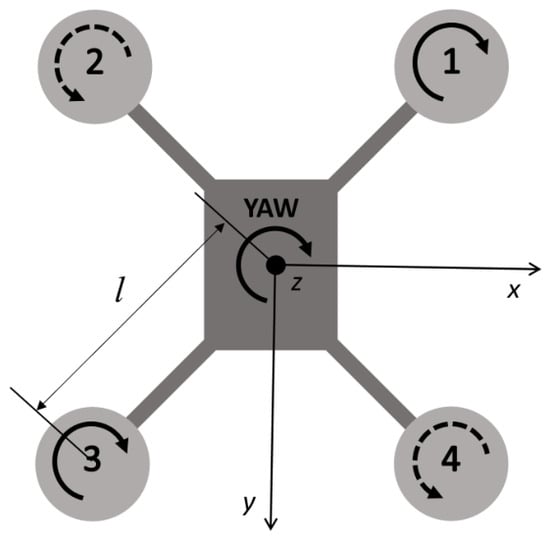
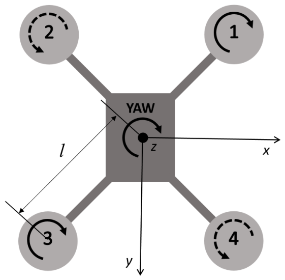
Figure 1 displays the X-configuration quadrotor utilized for this simulation framework. To enable steering around the yaw axis, the rotational direction of blades 2 and 4 is inverted compared to blades 1 and 3.

Figure 1. Drawing of the quadrotor in X configuration.

2.1. Dynamics Modeling of a Quadrotor UAV

Because this study aims to introduce the better kinematical reconstruction of the UAV’s position and attitude for forward dynamics simulation framework, intricate aerodynamic effects are omitted. Consequently, we assume that both the axial thrust force $F_T$ and the aerodynamic drag torque ${\mathit{T}}_D$ are modeled purely as functions of the rotor’s angular velocity:

$$F_{Ti}=f\left({\omega }_i\right),$$

(1)

$${\mathit{T}}_{Di}=f\left({\omega }_i\right),$$

(2)

where ${\omega }_i$ represent the i-th rotor’s angular velocity. The proposed numerical model enables the simulation of more complex maneuvers with more complex phenomena (without any effects on the results and conclusion), but for the purpose of a better understanding of the algorithm, simpler examples with emphasized rotations around individual axes (typical maneuvers that cause problems for quadrotors) were taken.

Building on these assumptions, the translational dynamics part can be written as

$$m\dot{\mathit{v}}=\mathit{R}\left[\begin{array}{c}0\\ 0\\ {\displaystyle {\sum }_{i=1}^4}{F}_{Ti}\end{array}\right]+\left[\begin{array}{c}0\\ 0\\ mg\end{array}\right],$$

(3)

where m defines the quadrotor mass, $\mathit{v}$ is the UAV’s translational velocity expressed in the global (inertial) reference frame, $\mathit{R}$ serves as the rotation matrix representing the UAV attitude and g is the gravitational acceleration constant.

The rotation matrix $\mathit{R}$ can be constructed from a known quaternion by using equation [25]

$$\mathit{R}=2\left[\begin{array}{ccc}{q}_0^2+q_1^2-{\displaystyle \frac{1}{2}}& q_1{q}_2-q_0{q}_3& q_1{q}_3+q_0{q}_2\\ q_1{q}_2+q_0{q}_3& q_0^2+q_2^2-{\displaystyle \frac{1}{2}}& q_2{q}_3-q_0{q}_1\\ q_1{q}_3-q_0{q}_2& q_2{q}_3+q_0{q}_1& q_0^2+q_3^2-{\displaystyle \frac{1}{2}}\end{array}\right].$$

(4)

Alternatively, transforming Equation (3) into the UAV’s body-fixed reference frame yields

$$m\dot{{\mathit{v}}^{\prime }}=\left[\begin{array}{c}0\\ 0\\ {\displaystyle {\sum }_{i=1}^4}{F}_{Ti}\end{array}\right]+{\mathit{R}}^T\left[\begin{array}{c}0\\ 0\\ mg\end{array}\right]-m\tilde{\mathsf{\omega }}{\mathit{v}}^{\prime },$$

(5)

where ${\mathit{v}}^{\prime }$ and $\mathsf{\omega }$ denote the translational and angular velocities of the UAV, respectively, mapped within the body-fixed coordinate system.

The rotational dynamics of the quadrotor UAV is governed by

$$\mathit{J}\dot{\mathsf{\omega }}={\displaystyle \sum _{i=1}^4}{\mathit{T}}_{Ti}+{\displaystyle \sum _{i=1}^4}{\mathit{T}}_{Di}-\tilde{\mathsf{\omega }}\mathit{J}\mathsf{\omega }-\tilde{\mathsf{\omega }}{\displaystyle \sum _{i=1}^4}{\mathit{J}}_{mi}{\mathsf{\omega }}_{mi},$$

(6)

the symbol $\mathit{J}$ represents the UAV inertia matrix, while ${\mathit{J}}_{mi}$ and ${\mathsf{\omega }}_{mi}$ account for the rotor inertia matrix and its angular velocity of the i-th rotor with respect to the vehicle. To determine the thrust torque, the formula ${\mathit{T}}_{Ti}={\sum }_{i=1}^4\widetilde{r_i}{F}_{Ti}$ is applied, utilizing $r_i$ to mark the origin of each rotor-fixed frame. We explicitly disregard the expression ${\sum }_{i=1}^4{\mathit{J}}_{mi}{\dot{\mathsf{\omega }}}_{mi}$ because the angular acceleration of the i-th rotor with respect to the UAV is assumed as sufficiently small. The entire formulation operates within the vehicle’s body-fixed reference frame.

Equations (3) (or (5)) and (6) can be solved by any numerical scheme for ordinary differential equations (ODEs) to obtain field of translational and angular velocities. Special attention must be dedicated to the kinematic reconstruction step, as it provides continuous tracking of the UAV’s position and, more challenging, its orientation.

2.2. Kinematic Reconstruction of the UAV Position and Attitude

The position of the UAV is described by position vector $\mathit{p}$, expressed in the global reference frame. While any standard ODE integration scheme can straightforwardly derive this state from the translational velocity, modeling the UAV’s attitude allows for various mathematical representations. Among these, utilization of rotational quaternions remains the prevailing methodology. One reason for that is the fact that they do not suffer from singularities when describing global 3D rotations, which all three-parameter descriptions (such as Euler angles) do. The other reason is that they are more intuitive for interpretation than SO(3) rotation matrices while also taking less space in the memory—four elements of the quaternion as opposed to nine elements in the rotation matrix.

The quaternion $\mathit{Q}$ is commonly considered as a four-element vector consisting of real part $q_0$ and imaginary part $\mathit{q}$, such that

$$\mathit{Q}=\left[\begin{array}{c}{q}_0\\ \mathit{q}\end{array}\right].$$

(7)

The (Hamiltonian) product of two quaternions can be defined in vector algebra notation as

$$\mathit{Q}\circ \mathit{P}=\left[\begin{array}{cccc}{q}_0& -q_1& -q_2& -q_3\\ q_1& q_0& -q_3& q_2\\ q_2& q_3& q_0& -q_1\\ q_3& -q_2& q_1& q_0\end{array}\right]\left[\begin{array}{c}{p}_0\\ p_1\\ p_2\\ p_3\end{array}\right].$$

(8)

Frequently designated as Euler parameters, the parameters of a rotational quaternion are naturally constrained to satisfy the unitary norm requirement, meaning that

$$\left|\left|\mathit{Q}\right|\right|=q_0^2+{\mathit{q}}^T\mathit{q}=1.$$

(9)

2.2.1. Method I: Conventional Approach to Kinematic Reconstruction of Quaternions

The conventional approach (used for example in [19,20,21,22,23,26]) to reconstruction of rotational quaternions from the angular velocity field is based on the equation [14]

$$\dot{\mathit{Q}}={\displaystyle \frac{1}{2}}\mathit{Q}\circ \mathsf{\omega }.$$

(10)

Together, these four linear differential equations and algebraic Equation (9) establish a DAE problem. This problem is typically addressed by applying an ODE solver to integrate (10), followed by an explicit normalization step via equation

$${\mathit{Q}}_{out}={\displaystyle \frac{\mathit{Q}}{\left|\left|\mathit{Q}\right|\right|}}.$$

(11)

However, as it will be presented in a numerical cases later in the paper, this approach may suffer because of non-preserving structure of Equation (10) during explicit integration since 3D rotations are inherently a nonlinear phenomenon. The four differential equations in (10) converge to the correct attitude for the decreasing time steps as expected, but their non-preserving structure may introduce errors that can cause the results’ drift from the correct solution at larger time steps, in spite of utilization of normalization step (11).

2.2.2. Method II: The Geometric Lie Group Approach to Kinematic Reconstruction of Quaternions

A new mathematical framework introduced in [18] effectively addresses these structural constraints. This formulation exploits the isomorphism that links unit quaternions to the unit sphere in ${\mathcal{R}}^4$, the symplectic group $Sp\left(1\right)$, and the special unitary group $SU\left(2\right)$. Consequently, unit quaternions can be characterized as elements of the sphere in ${\mathcal{R}}^4$ as

$${\mathcal{S}}^3=\left\{\mathit{Q}\in {\mathcal{R}}^4\mid \left|\left|\mathit{Q}\right|\right|=1\right\}.$$

(12)

Accordingly, a continuous curve on the unit sphere $\mathit{Q}\left(t\right)\in {\mathcal{S}}^3$ can be employed to characterize the UAV’s rotation. The velocity vectors, in contrast, are embedded in the space of the skew symplectic quaternions

$$sp\left(1\right)=\left\{\mathit{w}\in {\mathcal{R}}^4\mid \mathit{w}+\overline{\mathit{w}}=\mathbf{0}\right\},$$

(13)

where $\overline{\mathit{w}}$ represents conjugate of the quaternion $\mathit{w}$. The Lie algebra of the symplectic group $Sp\left(1\right)$ is denoted as $sp\left(1\right)$ (13), which comprises the set of pure quaternions. This algebraic structure exhibits an isomorphism to ${\mathcal{R}}^3$ and, consequently, to $so\left(3\right)$–the Lie algebra associated with the special orthogonal group $SO\left(3\right)$ governing 3D rotations. To guarantee this isomorphic relationship across the Lie algebras, a vector $\mathit{u}\in {\mathcal{R}}^3$ is mapped to the corresponding element $\mathit{w}={\displaystyle \frac{1}{2}}{\left[\begin{array}{cc}0& {\mathit{u}}^T\end{array}\right]}^T\in sp\left(1\right)$ [25] as well as to $\tilde{\mathit{u}}\in so\left(3\right)$. Here, the notation $\widetilde{·}$ stays for the skew-symmetric operator, such that [27]

$$\tilde{\mathit{u}}=\left[\begin{array}{ccc}0& -u_3& u_2\\ u_3& 0& -u_1\\ -u_2& u_1& 0\end{array}\right].$$

(14)

Due to the presented isomorphisms, similarly to exponential mapping on the $SO\left(3\right)$ group used in [28], the closed-form exponential mapping from vector $\mathit{u}$ to ${\mathcal{S}}^3$, i.e., ${\exp }_{{\mathcal{S}}^3}:{\mathcal{R}}^3\cong sp\left(1\right)\to Sp\left(1\right)\cong {\mathcal{S}}^3$ can be found as [18,25]

$${\exp }_{{\mathcal{S}}^3}\left(\mathit{w}\right)=\cos \left({\displaystyle \frac{1}{2}}\left|\left|\mathit{u}\right|\right|\right)\left[\begin{array}{c}1\\ \mathbf{0}\end{array}\right]+{\displaystyle \frac{\sin \left(\frac{1}{2}\left|\left|\mathit{u}\right|\right|\right)}{\left|\left|\mathit{u}\right|\right|}}\left[\begin{array}{c}0\\ \mathit{u}\end{array}\right].$$

(15)

The quaternion expressing a rotation about the vector $\mathit{u}$ by a magnitude of $\left|\left|\mathit{u}\right|\right|$ is generated via Equation (15). This mathematical relationship serves as the foundation for developing a kinematic procedure to derive rotational quaternions $\mathit{Q}$ from the angular velocity field $\mathsf{\omega }$. The procedure begins by determining an incremental rotation vector $\mathit{u}$, which is computed by the utilization of differential exponential operator [29,30] in the equation

$$\dot{\mathit{u}}={\mathrm{dexp}}_{-\tilde{\mathit{u}}}^{-1}\left(\mathsf{\omega }\right)=\mathsf{\omega }+{\displaystyle \frac{1}{2}}\tilde{\mathit{u}}\mathsf{\omega }-{\displaystyle \frac{\left|\left|\mathit{u}\right|\right|\cot \left(\frac{\left|\left|\mathit{u}\right|\right|}{2}\right)-2}{2{\left|\left|\mathit{u}\right|\right|}^2}}{\tilde{\mathit{u}}}^2\mathsf{\omega },$$

(16)

and then reconstructing the attitude by using Equation (15). The reconstruction algorithm based on (15) and (16) is 3D rotation structure preserving integration scheme expressed via quaternions. The other approach to mitigate the problems that arise when using conventional approach (Method I) is to use dual quaternion formulation. This means that, instead of solving for translations and rotations separately, the whole six-DOF rigid body motion will be parameterized by dual quaternions.

2.2.3. Method III: Dual Quaternions as a Lie Group Description of the Complete UAV 6-DOF Rigid Body Motion

To model complete rigid-body kinematics, dual quaternions offer a seamless generalization of traditional rotational quaternions. Mirroring the mathematical formulation of dual numbers, a dual quaternion $\widehat{\mathit{Q}}$ is expressed as [31]

$$\widehat{\mathit{Q}}=\mathit{Q}+\epsilon {\mathit{Q}}_{\epsilon }=\left[\begin{array}{c}{q}_0+\epsilon q_{\epsilon 0}\\ \mathit{q}+\epsilon {\mathit{q}}_{\epsilon }\end{array}\right],$$

(17)

where $\mathit{Q}$ and ${\mathit{Q}}_{\epsilon }$ are two quaternions, while $\epsilon$ is the dual unit satisfying condition ${\epsilon }^2=0$. Valid representation of rigid motion requires dual quaternions to possess a unitary norm, a condition that gives rise to the relation [25]

$$\left|\left|\widehat{\mathit{Q}}\right|\right|=\left|\left|\mathit{Q}\right|\right|+\epsilon 2{\mathit{Q}}^T{\mathit{Q}}_{\epsilon }=1+\epsilon 0.$$

(18)

In other words unit dual quaternion has to satisfy two constraints: unitary norm of the quaternion $\left|\left|\mathit{Q}\right|\right|=1$ and orthogonality of two quaternions ${\mathit{Q}}^T{\mathit{Q}}_{\epsilon }=0$, also known as Plücker condition.

Analogous to the way unit quaternions constitute an $Sp\left(1\right)$ Lie group, unit dual quaternions establish the six-dimensional Lie group $\widehat{Sp}\left(1\right)$ by substituting dual elements into the original $Sp\left(1\right)$ framework. Because the $\widehat{Sp}\left(1\right)$ group is isomorphic to $SE\left(3\right)$, it serves as an effective mathematical tool for representing spatial rigid body displacements. Furthermore, the dual pure quaternions form the $\widehat{sp}\left(1\right)$ Lie algebra, which can be directly mapped to $se\left(3\right)$ due to their isomorphic equivalence

$$\mathit{X}=\left[\begin{array}{c}\mathit{u}\\ \mathsf{\eta }\end{array}\right]\in se\left(3\right)\to \widehat{\mathit{X}}={\displaystyle \frac{1}{2}}\left[\begin{array}{c}0\\ \mathit{u}+\epsilon \mathsf{\eta }\end{array}\right]\in \widehat{sp}\left(1\right).$$

(19)

Leveraging this isomorphic equivalence, the exponential map for a unit dual quaternion that parameterizes rigid motion can be formulated as [32]

$${\exp }_{{\widehat{\mathcal{S}}}^3}\widehat{\mathit{X}}={\exp }_{{\mathcal{S}}^3}\left(\mathit{w}\right)+\epsilon \left[\begin{array}{c}-{\displaystyle \frac{d}{2}}\sin \left({\displaystyle \frac{1}{2}}\left|\left|\mathit{u}\right|\right|\right)\\ {\displaystyle \frac{d}{2}}\cos \left({\displaystyle \frac{1}{2}}\left|\left|\mathit{u}\right|\right|\right)\mathbf{n}+\sin \left({\displaystyle \frac{1}{2}}\left|\left|\mathit{u}\right|\right|\right)\mathit{m}\end{array}\right],$$

(20)

where $\mathit{n}=\mathit{u}/\left|\left|\mathit{u}\right|\right|$ is the unit vector along the screw axis, $\mathit{m}$ is the moment vector defined as $\mathit{m}=-\mathit{n}\times \left(-\mathit{n}\times \mathsf{\eta }\right)/\left|\left|\mathit{u}\right|\right|$, while d is displacement along the screw axis $d=\mathit{u}·\mathsf{\eta }/\left|\left|\mathit{u}\right|\right|=\mathit{n}·\mathit{m}$. The non-dual part of (20) functions as the orientation-defining unit quaternion established in the prior section, whereas spatial translation is expressed in the dual part.

The abovementioned structure-preserving procedure can be used for kinematic reconstruction of whole rigid motion from the velocity field, now consisting of both translational and angular velocities. The incremental screw coordinates can be found by solving differential equation

$$\dot{\mathit{X}}={\mathrm{dexp}}_{-\tilde{\mathit{u}}}^{-1}\left(\mathit{V}\right),$$

(21)

where the vector containing both the angular and linear velocities is designated as $\mathit{V}={\left[\begin{array}{cc}{\mathsf{\omega }}^T& {\mathit{v}}^T\end{array}\right]}^T$, resolved entirely within the body-fixed reference frame. For the closed form of Equation (21), see [25,33,34], for example.

In brief, Methods I and II evaluate identical governing dynamics: Newton equation for translational dynamics expressed in the global (fixed) reference frame and Euler equations for computing angular velocity field, expressed in the body-fixed reference frame. Conversely, Method III projects both the translational and rotational equations of motion directly onto the vehicle’s body-fixed reference frame. Crucially, the transformation of the translational governing equations between the global and body-fixed reference frames is mathematically exact. Because this coordinate transformation introduces no geometric truncations, modeling simplifications, or numerical formulation errors, the change of reference frame itself does not inherently affect the precision of the solution. Consequently, after obtaining translational and angular velocity fields, Methods I and II deal with kinematic reconstruction of position and velocity separately, while Method III treats translation and rotation as a coupled rigid motion via dual quaternions. Therefore, the performance of Method III should be interpreted as that of the overall coupled formulation. Any observed differences in accuracy stem not only from this algebraic coupling and the intrinsic properties of the dual quaternion kinematic reconstruction, but also from the choice of the reference frame for the dynamical equations, such as the body-fixed Newton equation.

3. Numerical Experiments

In this section, numerical experiments are conducted in order to evaluate the methods described in Section 2. It should be emphasized that the discussion in this chapter depends on the specific numerical representation. While some results exhibit an excellent numerical match, minor discrepancies may exist due to accumulated numerical round-off errors. Put differently, our analysis disregards discrepancies that fall within the margin of double-precision floating-point round-off errors. Furthermore, the benchmark position and orientation for each test case are defined by the uniform converged solution yielded by all described methods.

In order to allow for evaluation and comparison of the results, the metrics for evaluating position and attitude error need to be defined. The position error is defined as the Euclidean norm of the vector describing the difference between the obtained and correct position. For the rotation, the task of choosing a metric is more challenging. Here, similarly to the position, the Euclidean norm of the difference between the obtained and correct quaternion is adopted as the metric for describing the error in attitude. Although this metric is not the only meaningful metric that could be adopted for the orientation error, the conclusions drawn in this paper remain consistent, as any other sensible metric would yield the same comparative outcomes. Consequently, while the plots and values might vary slightly, the overall assessment and comparison of the methods remain unchanged. In the following numerical experiments, no quaternion sign switching occurs, and the same branch is consistently used for both reference and computed solutions, thereby ensuring the validity of the adopted metric.

Following the definition of these evaluation metrics, the proposed methodology is applied to a specific aircraft configuration. As previously established, the selected quadrotor operates in an X configuration layout, with properties given in Table 1. The properties of the chosen X-configuration quadrotor were measured and derived from a setup representing a typical commercially available, custom-built First-Person View (FPV) drone, consisting of a QAV250 carbon-fiber racing frame (with 6” extended arms). Within this dataset, the arm length denotes the horizontal span from the aircraft’s center of mass to the rotor’s centerline, whereas the rotor–motor assembly inertia characterizes the total moment of inertia of the spinning components about their rotation axis. Ultimately, all governing ODEs are integrated numerically using a fourth-order Runge–Kutta method.

Table 1. Properties of the chosen quadrotor in X-configuration.

Description	Label	Value
mass	m	$0.5$
inertia matrix	$\mathit{J}$	$\left[\begin{array}{ccc}0.00365& 0& 0\\ 0& 0.00368& 0\\ 0& 0& 0.00703\end{array}\right]$
arm length	l	$0.17$
rotor-motor assembly inertia	$J_{mzi}$	$0.0002271$
thrust force	$\left|F_{Ti}\left({\omega }_{mi}\right)\right|$	$5.57·{10}^{-6}·{\omega }_{mi}^2$
drag torque	$\left|{\mathit{T}}_{Di}\left({\omega }_{mi}\right)\right|$	$\left[\begin{array}{c}0\\ 0\\ -1.37·{10}^{-7}·\left|{\omega }_{mi}\right|·{\omega }_{mi}\end{array}\right]$

3.1. Test Case I—Yaw Rotation

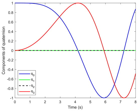
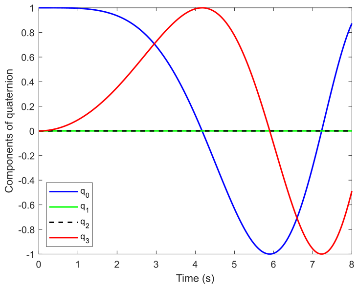
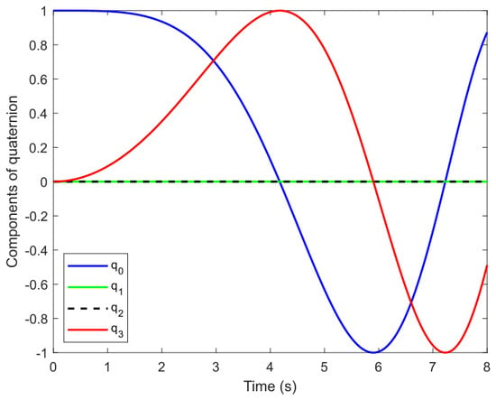
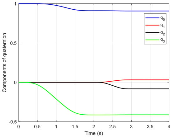
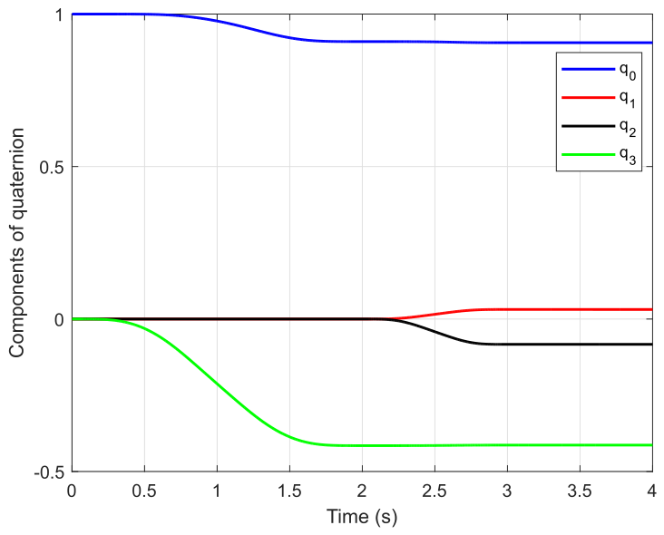
For the first test case, the simplest rotation that could possibly be envisioned for a quadrotor UAV is chosen. This is the rotation about the vertical, z axis, also known as yaw axis. This is done by rotating rotors 1 and 3 with different angular velocities than rotors 2 and 4 (depicted in Figure 1) while keeping the total thrust force required to ensure hovering of the UAV. The length of the simulation is set to 8 s and the resulting evolution of quaternion elements in time is given in Figure 2.

Figure 2. Components of the quaternion in time for yaw rotation.

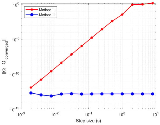
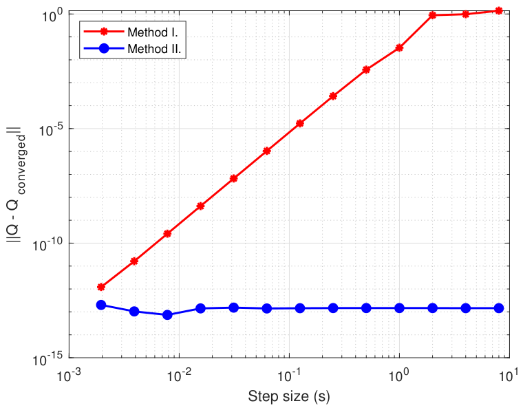
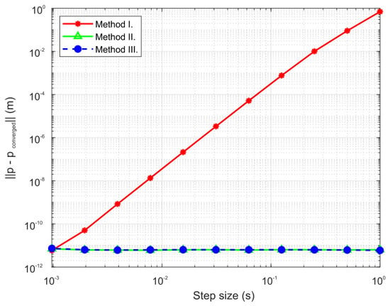
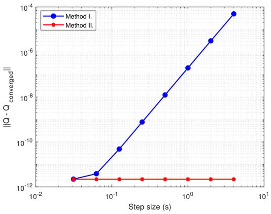
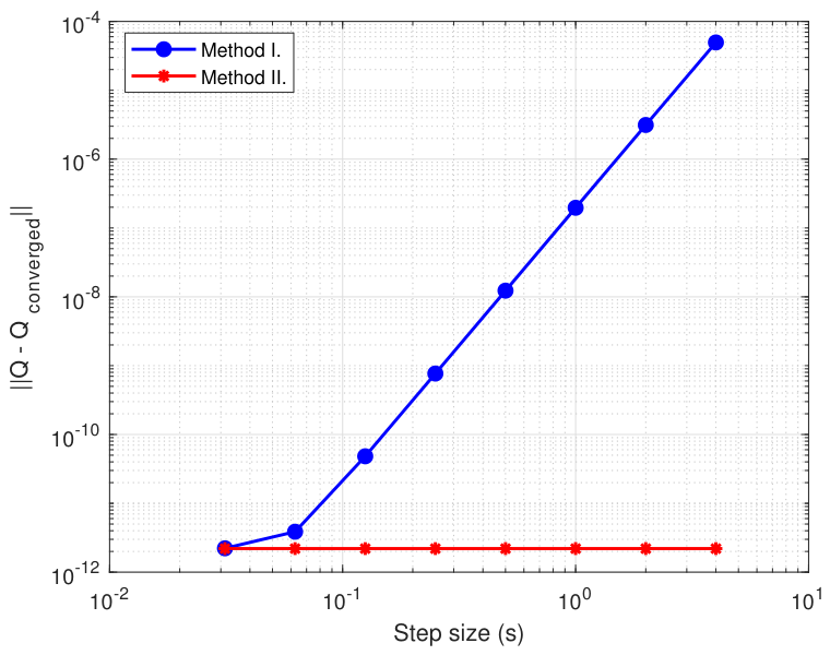
Methods I and II are used and compared for the given test case, while Method III is omitted, since there is no translation involved in this motion. Both methods converge to the same solution for step size equal to ${10}^{-3}$. To compare methods, the results of the quaternion at the end of simulation for the increasing time steps are compared with the converged solution. The comparison is given in Figure 3 in terms of the norm of the difference between resulting and converged quaternion.

Figure 3. Norm of the difference between converged and resulting quaternion for increasing step size.

It is important to note that both methods integrate completely the same equations for dynamics (6) and the difference is arising solely from different approaches to the kinematic reconstruction. Method I exhibits usual, well-known convergence to the correct solution with a decreasing step size, while Method II is exact for the presented motion case with any tested step size. The errors introduced with Method I arise from non-structure preservation of the rotation phenomenon in Equation (10), while Method II utilizes more natural, and obviously better, approach to reconstructing incremental rotation (16).

3.2. Test Case II—Yaw Rotation Coupled with Climbing

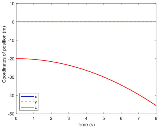
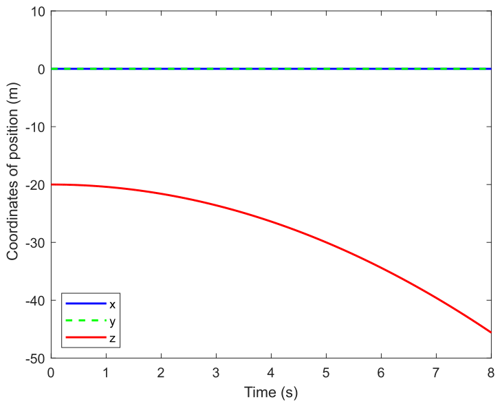
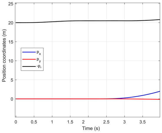
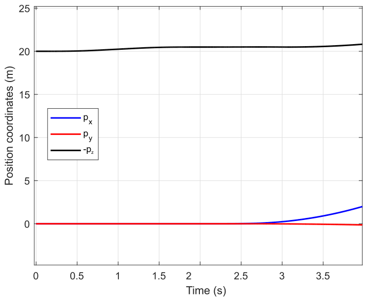
In addition to yaw rotation presented in Section 3.1, this test case also involves climbing of the UAV. This flight condition is achieved by operating rotors 1 and 3 at different angular rates than rotors 2 and 4, though in this scenario, the cumulative thrust must exceed the total weight of the UAV. The length of the simulation is again set to 8 and the results for the evolution of position coordinates and quaternion elements in time are depicted in Figure 4 and Figure 5.

Figure 4. Coordinates of the position in time for test case II.

Figure 5. Components of the quaternion in time for test case II.

All three presented methods were tested and compared in this test case. All three algorithms involve solving the same Euler equations for rotational dynamics (6). However, Method III involves solving the Newton equations for translational dynamics in the body-fixed reference frame (5), while Methods I and II solve the Newton equations in the global (fixed) reference frame (3). At an integration step size of ${10}^{-3}$, every tested method converged to the same solution. Subsequently, to assess robustness, the methods are tested for increasing step sizes and the results are compared to the converged solution.

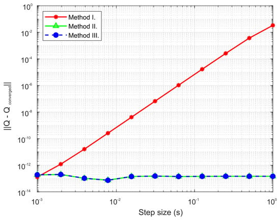
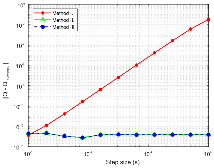
Figure 6 illustrates the norm of the position error vector across increasing step size for all three tested methods, whereas the corresponding deviation between the converged and resulting quaternions for increasing step size is plotted in Figure 7. The data reveals that Method I follows a typical convergence path toward the correct solution, both in position and attitude, as expected. Conversely, Methods II and III deliver accurate outputs regardless of the selected time step. Notably, since Methods I and II compute translational states via identical dynamic and kinematic formulations, their divergence stems exclusively from the kinematic reconstruction of rotation. Consequently, the performance degradation of Method I highlighted in Figure 7 originates entirely from inaccuracies in updating the attitude from the angular velocity field. This leads to the flawed calculation of the force vector in global reference frame, since it depends on the UAV attitude as seen in the Equation (3), finally leading to the errors in the position calculation. The attitude reconstruction from the velocity field utilized in Method III is equivalent to reconstruction in Method II and the overall results for this test case obtained by Methods II and III are equal and no difference can be made between them.

Figure 6. Norm of the position error vector for increasing step size.

Figure 7. Norm of the difference between converged and resulting quaternion for increasing step size.

3.3. Test Case III—Roll Maneuver

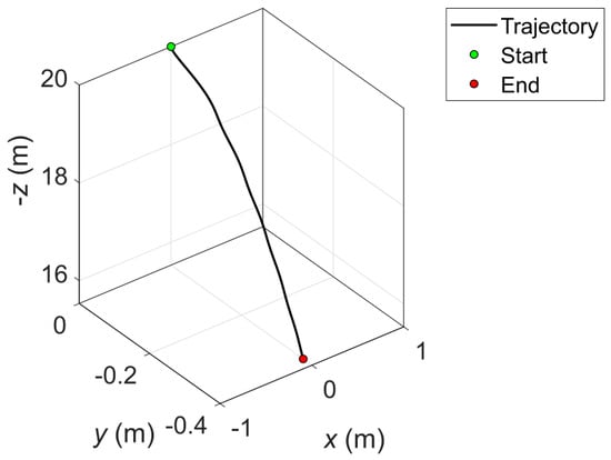
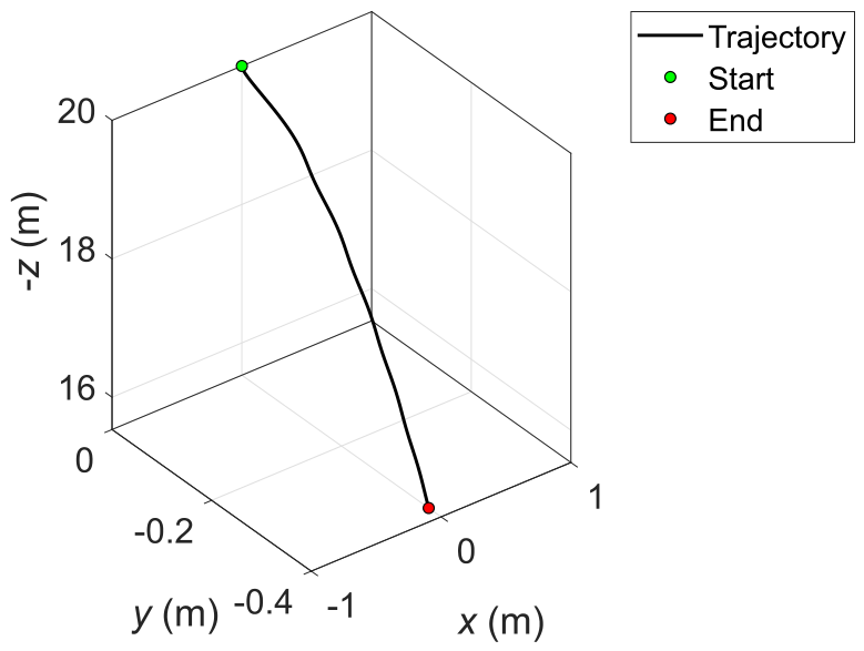
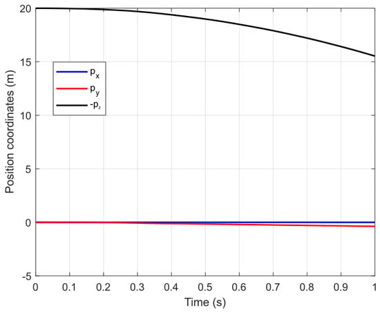
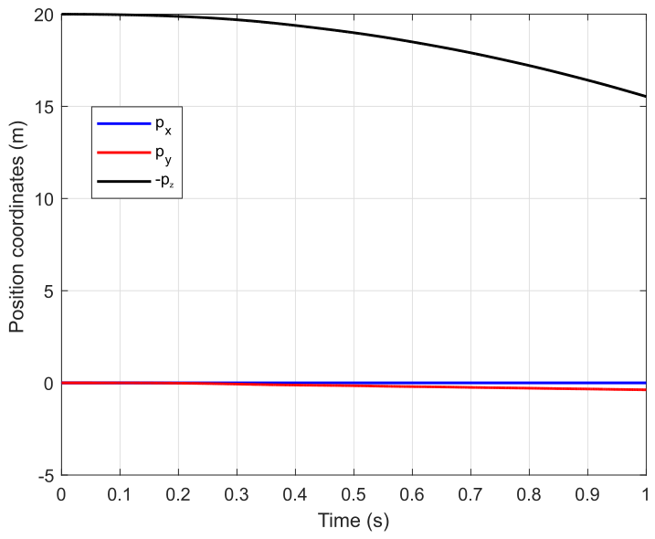
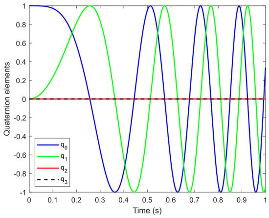
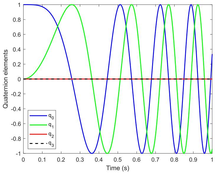
This section explores a slightly more complex maneuver. The UAV begins in a hovering state at an altitude of 20 m, whereupon rotors 1 and 2 are accelerated concurrently with the deceleration of rotors 3 and 4; this input triggers a roll maneuver, causing the aircraft to rotate about its local x axis. The UAV trajectory is depicted in Figure 8, while the position and quaternion evolution in time are shown in Figure 9 and Figure 10.

Figure 8. Trajectory of the UAV performing roll maneuver.

Figure 9. Coordinates of position in time for roll maneuver.

Figure 10. Quaternion components in time for roll maneuver.

The overall simulation duration is set to 1 s, with the UAV motion computed by using all three outlined methods.

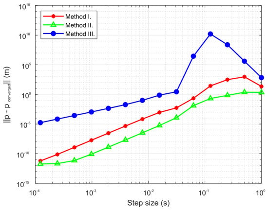
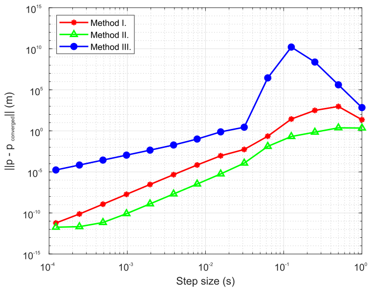
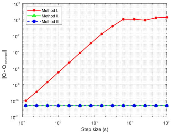
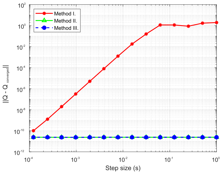
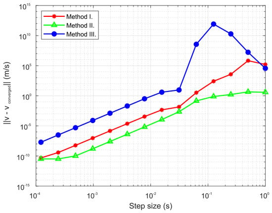
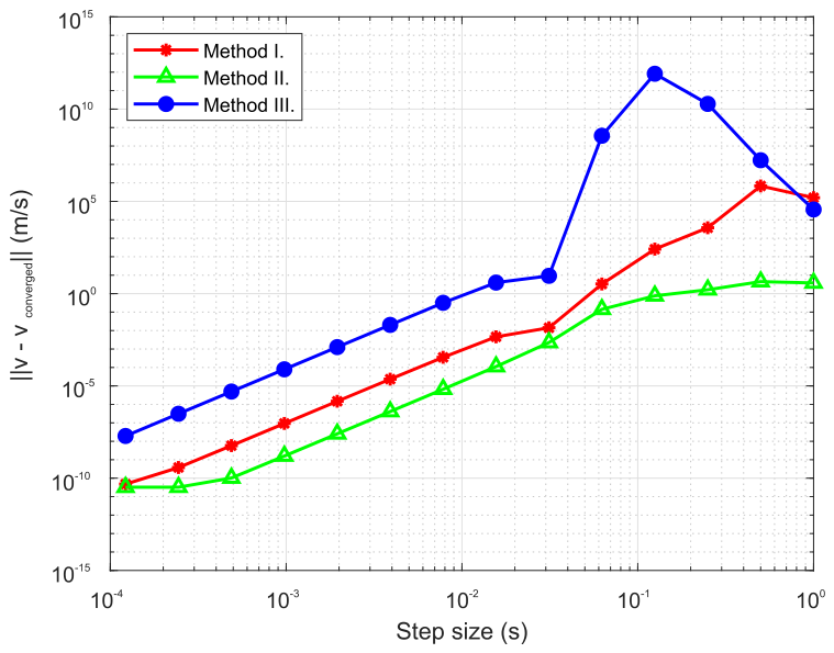
For both position and attitude, Methods I and II reached the same converged outputs at a discretization step of ${10}^{-4}$. However, Method III needed step size below ${10}^{-6}$ to achieve complete convergence of the position coordinates. To assess error propagation, the trajectories generated across expanding time-step selections are benchmarked against the converged baseline, evaluating both the position error vector norm and the corresponding quaternion deviation norm. This comparative analysis is charted in Figure 11 and Figure 12.

Figure 11. Norm of the position error vector for increasing step size.

Figure 12. Norm of the difference between converged and resulting quaternions for increasing step size.

Because they yield exact solutions independent of the discretization interval (independent of the step size), the Lie group schemes (Methods II and III) remain superior for reconstructing the UAV’s attitude from angular velocity inputs. In contrast, while the standard Method I demonstrates convergence to the correct solution under reducing step sizes, its output becomes completely useless at larger step values.

Regarding position integration, none of the methods delivered accurate solutions under very large time steps, though all methods demonstrated proper convergence as the step sizes were reduced. Nonetheless, a substantial difference in accuracy is visible among the methods. Method II clearly outperforms the other tested methods, proving to be the most accurate choice across all evaluated discretization patterns. In fact, its performance is superior by at least two orders of magnitude than the other methods for the majority of the tested step sizes. As previously noted, Methods I and II update positions through identical routines; therefore, the divergence in their results stems solely from the fact that Method II provides a much better kinematic reconstruction of the attitude from the angular velocity field.

Conversely, the dual-quaternion-based Method III is highly susceptible to numerical instabilities at larger step sizes, demonstrating the slowest convergence toward the correct solution. This due to the fact that Method III evaluates the Newton equation by utilizing the body-fixed reference frame (5) in order to capture coupled rigid-body motion; this governing relation is inherently more intricate than its counterpart expressed in the global reference frame (3). This leads to errors in the calculation of the UAV velocity, as can be seen from Figure 13 showing the norm of the error in calculating velocity with different methods for increasing step sizes. Once again, despite both Methods I and II integrating the identical Newton equation for translational dynamics (3), the Lie group framework of Method II delivers better results. This outcome arises because the translational formulation is coupled with the rotational quaternion, which is more accurately reconstructed using Method II.

Figure 13. Norm of the velocity error vector for increasing step size.

3.4. Test Case IV—Orbit Maneuver

It is obvious that Methods II and III exhibit superior behavior in terms of attitude reconstruction for the above presented test cases, when compared to Method I. Additionally, Method II exhibited the best performance in terms of position calculation for the presented test cases. However, the test cases I–III included planar maneuvers, and general three-dimensional test cases should be analyzed to demonstrate (although this is clear from the mathematical expression (16)) that the method benefits are not constrained to 2D numerical examples.

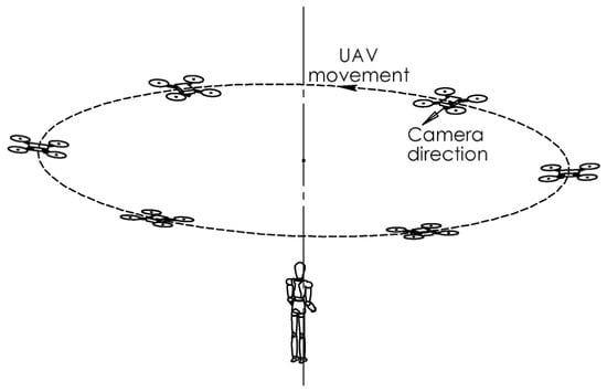
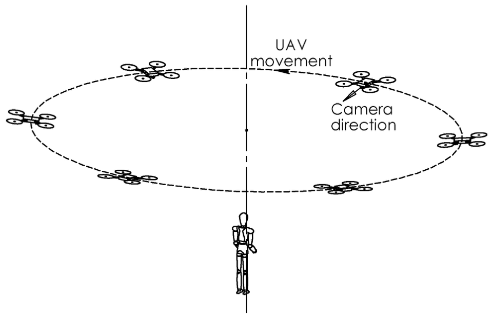
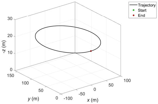
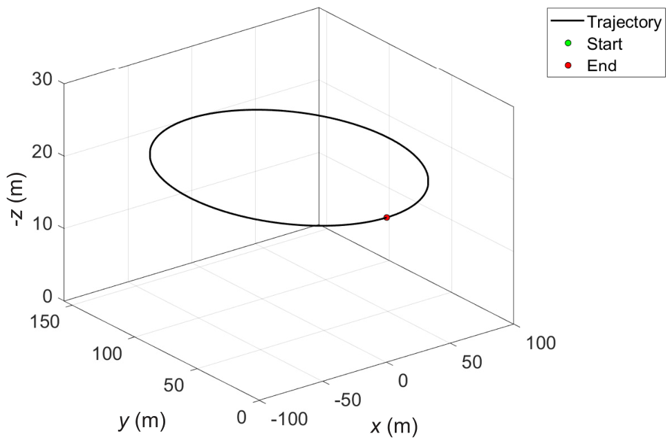
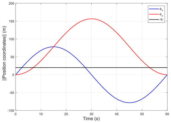
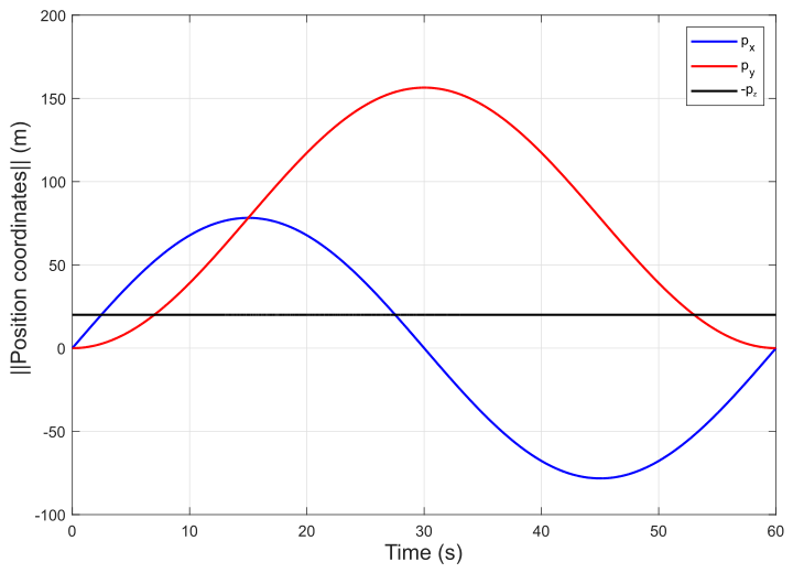
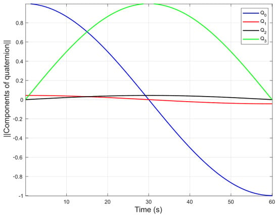
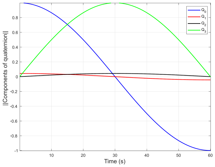
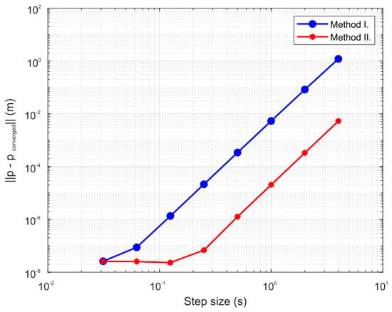
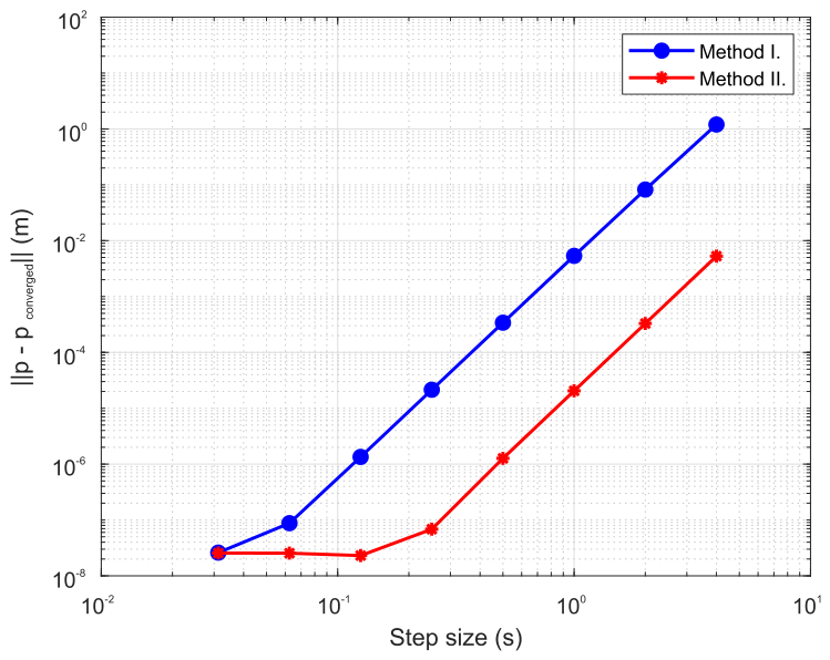
In this section, performance of Methods I and II is compared in the example of an orbit maneuver, illustrated in Figure 14. Here, the UAV is orbiting around and pointing towards a fixed object—the maneuver that is often employed when recording a video. In this example, the UAV is orbiting with a period of 60 s, at a fixed altitude of 20 m. The maneuver is depicted in Figure 15, while Figure 16 and Figure 17 show the resulting time evolution of position coordinates and quaternion components. One full orbit is simulated and both methods converged to the same solution for a time step of ${10}^{-2}$ s. Same as for the other analyzed test cases, the methods are then compared based on the accuracy at different time step sizes. The norm of the position error vector and the norm of the difference between the converged and resulting quaternions for different step sizes are shown in Figure 18 and Figure 19.

Figure 14. Sketch of the UAV orbiting around and pointing towards a fixed object.

Figure 15. Trajectory of the UAV performing orbit maneuver.

Figure 16. Time evolution of position coordinates for orbit maneuver.

Figure 17. Time evolution of quaternion components for orbit maneuver.

Figure 18. Norm of the position error vector for increasing step size.

Figure 19. Norm of the difference between converged and resulting quaternion for increasing step size.

As presented in Figure 19, the Method II is again performing an exact attitude reconstruction for any tested time step, although the analyzed test case is not planar (i.e., the rotation axis is not collinear with principal inertia axis). However, the fact that the rotation axis is not changing direction during the orbiting maneuver allows for the exact calculation of UAV dynamics and this emphasizes the errors that Method I exhibits in attitude reconstruction that are not observed for Method II.

It is important to note again that both presented methods capture the constant angular velocity field exactly, and the errors visible for Method I are introduced by non-structure preservation of the kinematical update step in (10), compared to the nonlinear kinematical update step for Method II, expressed by (16).

Additionally, despite the fact that the position update is performed with exactly the same algorithm for Methods I and II, Method II performs a significantly better (by more than two orders of magnitude for larger time steps) position calculation, as presented in Figure 18. This is due to the fact that errors in determining orientation, introduced within kinematical reconstruction of Method I give rise to the errors in calculating force vector because the direction of force vector is directly dependent on the orientation of the propellers.

3.5. Test Case V—3D Maneuver with Changing Angular Velocity

In order to further demonstrate the attitude reconstruction superiority of Method II, when compared to Method I, a random 3D maneuver is chosen. The time evolution of position coordinates and quaternion elements for the chosen maneuver is presented in Figure 20 and Figure 21.

Figure 20. Time evolution of position coordinates for a chosen 3D maneuver.

Figure 21. Time evolution of quaternion components for a chosen 3D maneuver.

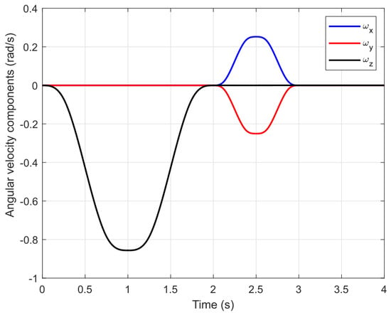
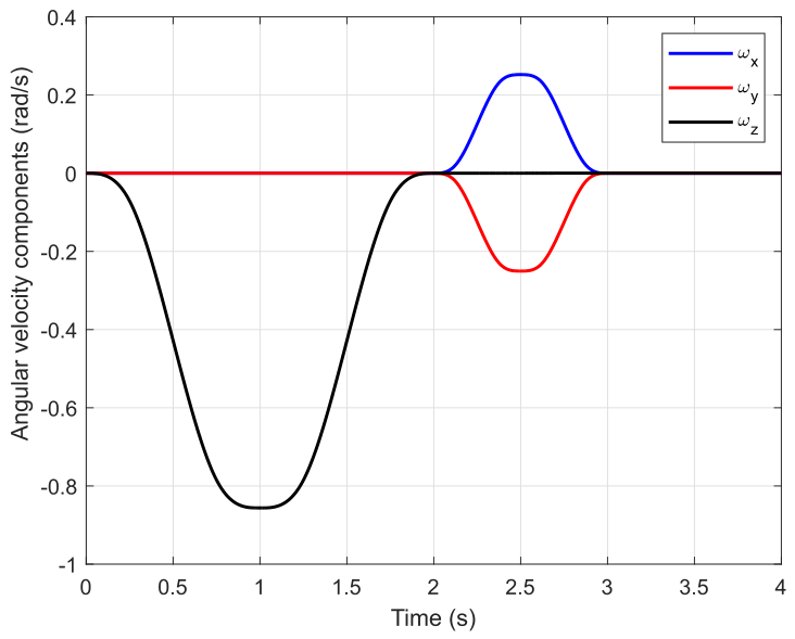
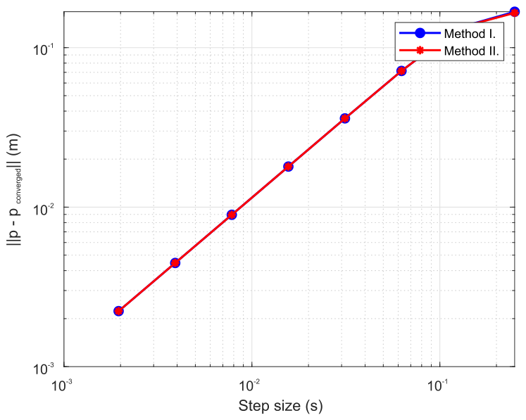
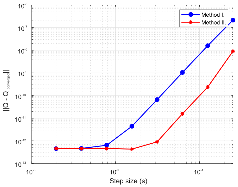
Since the main focus of the paper is attitude reconstruction, with the aim of eliminating errors arising from the rotational dynamics simulation, the converged angular velocity field has been stored and the converged values have been used in the simulation with both methods. The resulting time evolution of the angular velocity components is presented in Figure 22. The same comparison methodology is used as for the previous test cases. Methods I and II converged to the same quaternion for the time step of $2^{-8}$. The norm of the position error vector and the norm of the difference between the converged and resulting quaternions for different step sizes are shown in Figure 23 and Figure 24.

Figure 22. Time evolution of angular velocity components for a chosen 3D maneuver.

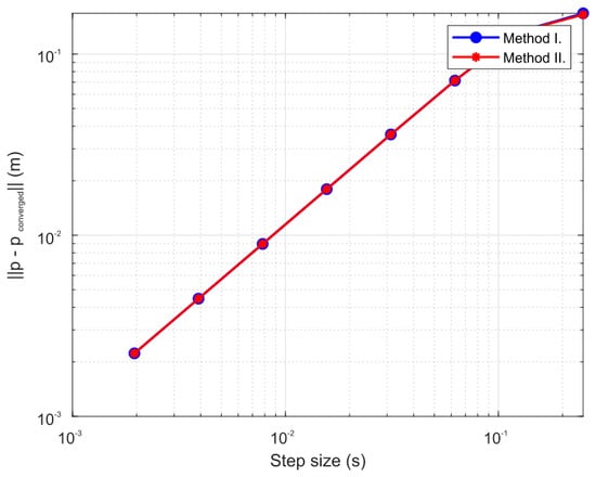
Figure 23. Norm of the position error vector for increasing step size.

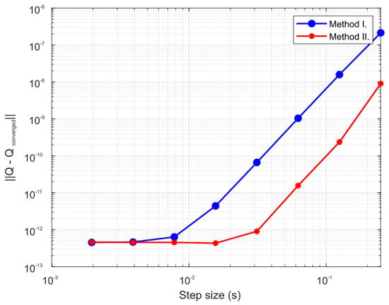
Figure 24. Norm of the difference between converged and resulting quaternion for increasing step size.

Both methods performed equally on the position vector calculation, and the results presented in Figure 23 do not include converged time steps, since the plots and computation time would be larger without any added value. As clearly visible in Figure 24, Method II is superior in attitude reconstruction when compared to Method I by almost two orders of magnitude. It is important to note that this is only due to the better attitude reconstruction, since both methods used the same (converged) solution of the angular velocity field. The Method I again suffers from the errors introduced by non-structure preservation of the kinematical update step (10), which is avoided by using a structure-preserving kinematical update based on (15) and (16) in Method II. This example provides a valuable information about the benefits of using recently proposed geometrical methods for tasks of reconstructing orientation from a known (often measured by onboard sensor) angular velocity field, where the standard methods may introduce errors that are circumvented if geometrical method for attitude reconstruction are used.

4. Conclusions

The paper establishes an evaluation of the recently introduced quaternion-based geometric integration algorithms for forward dynamics simulation in the quadrotor UAV framework. The geometric 3D rotation structure-preserving algorithms are based on Lie group kinematic reconstruction techniques for rotation or for both position and rotation updates. The geometric algorithms are benchmarked against the algorithm conventionally used for solving UAV forward dynamics problem, when quaternions are used as parameters for describing rotations. The methods are evaluated by using five numerical test cases.

The numerical results demonstrate that the described geometric methods are superior to the conventional method in describing rotations of the UAV due to the better reconstruction of the attitude from the angular velocity field. The method which updates rotations by using a geometric algorithm and translations in the conventional way (Method II) delivered the best performance on presented test cases in terms of position update. On the other hand, in test cases I–III, the geometric algorithm describing the whole rigid motion in a coupled manner by using integration on dual quaternions (Method III) demonstrated performance variations when compared to the conventional method (Method I). This is because of the trade-off between better description of the rotation update and more complex formulation of the Newton differential equation.

The evaluation establishes that the geometric methods consistently match or exceed the accuracy of the conventional method when neglecting round-off errors (see Table 2). In addition, the geometric algorithm updating rotation using the Lie group method and translation by using the conventional method is also superior in updating positions due to the same or better rotational update, together with equivalent translation update. On the other hand, the method describing the rigid motion in a coupled manner, by using dual quaternions, presents variational characteristics in terms of position update when compared to the conventional method, as shown in the presented test cases.

Table 2. Features and results of the three methods evaluated using five numerical test cases.

Test Case	Method I	Method II	Method III
Features	Conventional Approach to Kinematic Reconstruction of Quaternions	Geometric (Lie Group) Approach to Kinematic Reconstruction of Quaternions	Dual Quaternions as a Lie Group Description of the Complete UAV Rigid Motion
Test case I—Yaw rotation	convergence to the correct solution with a decreasing step size	exact solutions for any tested step size	omitted
Test case II—Yaw rotation coupled with climbing	convergence to the correct solution, both in position and attitude	exact solutions for any tested step size	exact solutions for any tested step size
Test case III—Roll maneuver	convergence to the correct solution with a decreasing step size	exact solutions for any tested step size	exact solutions for any tested step size
Test case IV—Orbit maneuver	suffers from the errors introduced by non-structure preservation of the kinematical update step	exact attitude reconstruction for any tested time step	omitted
Test case V—3D maneuver with changing angular velocity	suffers from the errors introduced by non-structure preservation of the kinematical update step	superior in attitude reconstruction when compared to Method I by almost two orders of magnitude	omitted

To conclude, it is verified that the method for updating rotational quaternions by using the Lie group algorithm (Method II) does not require significant changes to the conventional code (Method I) for simulating forward dynamics, which uses quaternions as the parameters describing attitude.

Regarding future work, several avenues of research will be pursued to build upon the insights gained from this study. First, the practical implementation of the proposed kinematic reconstruction integration procedures will be developed for the real-time attitude estimation of quadrotor UAVs. To validate the simulation models under realistic computational constraints, these algorithms will be deployed and tested in real-time on a single-board computer or SBC (e.g., Raspberry Pi). Furthermore, physical experiments will be conducted using open-architecture quadrotor UAV platforms. This experimental phase will focus on developing advanced controllers that fully utilize the recently introduced attitude and position update algorithms based on Lie groups for modeling the underlying dynamics of the UAV. These steps will bridge the gap between theoretical geometric integration and robust, real-world flight control applications.

References

- Hoffman, D.; Rehan, M.; MacKunis, W.; Reyhanoglu, M. Quaternion-Based Robust Trajectory Tracking Control of a Quadrotor Hover System. Int. J. Control Autom. Syst. 2018, 16, 2575–2584. [Google Scholar] [CrossRef] [Scilit]
- Al-Younis, Y.; El-Khasawneh, B.; Al-Sartawi, M. Quaternion-Based Robust Sliding-Mode Controller for Quadrotors Operating under Wind Disturbances. Aerospace 2025, 12, 93. [Google Scholar] [CrossRef] [Scilit]
- Li, R.; Yang, Z.; Yan, G.; Jian, L.; Li, G.; Li, Z. Robust Approximate Optimal Trajectory Tracking Control for Quadrotors. Aerospace 2024, 11, 149. [Google Scholar] [CrossRef] [Scilit]
- Zhang, T.; Wang, X.; Liu, Y. Robust Trajectory Tracking Control for Quadrotor UAVs with Prescribed Performance Constraints. J. Intell. Robot. Syst. 2025, 111, 45. [Google Scholar]
- Hartley, R.; Trumpf, J.; Dai, Y.; Li, H. Rotation Averaging. Int. J. Comput. Vis. 2013, 103, 267–305. [Google Scholar] [CrossRef] [Scilit]
- Etkin, B.; Reid, L.D. Dynamics of Flight: Stability and Control, 3rd ed.; John Wiley: New York, NY, USA, 1996. [Google Scholar]
- Stengel, R.F. Flight Dynamics, 2nd ed.; Princeton University Press: Princeton, NJ, USA, 2022. [Google Scholar]
- Holm, D.D. Geometric Mechanics. Part II: Rotating, Translating and Rolling, 2nd ed.; Imperial College Press: London, UK, 2011. [Google Scholar]
- Marsden, J.E.; Ratiu, T.S. Introduction to Mechanics and Symmetry; Texts in Applied Mathematics; Springer: New York, NY, USA, 1999; Volume 17. [Google Scholar]
- Holm, D.D.; Schmah, T.; Stoica, C. Geometric Mechanics and Symmetry: From Finite to Infinite Dimensions; Oxford Graduate Texts in Mathematics; Oxford University Press: Oxford, UK, 2009; Volume 12, Available online: https://academic.oup.com/book/53910 (accessed on 24 April 2023).
- Hall, B.C. Lie Groups, Lie Algebras, and Representations: An Elementary Introduction, 2nd ed.; Springer: Cham, Switzerland, 2015. [Google Scholar]
- Knapp, A.W. Lie Groups Beyond an Introduction, 2nd ed.; Birkhäuser: Boston, MA, USA, 2002. [Google Scholar]
- Serre, J.P. Lie Algebras and Lie Groups, 2nd ed.; Springer: Berlin/Heidelberg, Germany, 2006. [Google Scholar]
- Nikravesh, P.E. Computer-Aided Analysis of Mechanical Systems, 2nd ed.; Prentice-Hall: New Jersey, NJ, USA, 1988. [Google Scholar]
- Shabana, A.A. Dynamics of Multibody Systems, 5th ed.; Cambridge University Press: Cambridge, UK, 2020; p. 420. [Google Scholar]
- Erdmann, K.; Wildon, M.J. Introduction to Lie Algebras; Springer: London, UK, 2006. [Google Scholar]
- Choquet-Bruhat, Y.; DeWitt-Morette, C.; Dillard-Bleick, M. Analysis, Manifolds and Physics; Elsevier Science: Amsterdam, The Netherlands, 1982. [Google Scholar]
- Terze, Z.; Müller, A.; Zlatar, D. Singularity-free time integration of rotational quaternions using non-redundant ordinary differential equations. Multibody Syst. Dyn. 2016, 38, 201–225. [Google Scholar] [CrossRef] [Scilit]
- Du, H.; Zhu, W.; Wen, G.; Duan, Z.; Lü, J. Distributed Formation Control of Multiple Quadrotor Aircraft Based on Nonsmooth Consensus Algorithms. IEEE Trans. Cybern. 2019, 49, 342–353. [Google Scholar] [CrossRef] [Scilit]
- Castillo, A.; Sanz, R.; Garcia, P.; Qiu, W.; Wang, H.; Xu, C. Disturbance observer-based quadrotor attitude tracking control for aggressive maneuvers. Control Eng. Pract. 2019, 82, 14–23. [Google Scholar] [CrossRef] [Scilit]
- Xu, L.; Qin, K.; Tang, F.; Shi, M.; Lin, B. A Novel Attitude Control Strategy for a Quadrotor Drone with Actuator Dynamics Based on a High-Order Sliding Mode Disturbance Observer. Drones 2024, 8, 131. [Google Scholar] [CrossRef] [Scilit]
- Dou, J.; King, X.; Chen, X.; Wen, B. Output feedback observer-based dynamic surface controller for quadrotor UAV using quaternion representation. Proc. Inst. Mech. Eng. Part G J. Aerosp. Eng. 2017, 231, 2537–2548. [Google Scholar] [CrossRef] [Scilit]
- Zhang, X.; Liu, Y.; Wang, J.; Zhang, H. Quaternion-Based Non-Singular Terminal Sliding Mode Control with Dynamic Surface and Observer Framework for Quadrotor UAVs. Drones 2024, 8, 629. [Google Scholar]
- Terze, Z.; Zlatar, D.; Kasalo, M.; Andrić, M. Lie group quaternion attitude-reconstruction of quadrotor UAV. In International Conference on Geometric Science of Information; Springer: Cham, Switzerland, 2023; pp. 3–11. Available online: https://link.springer.com/chapter/10.1007/978-3-031-38299-4_1 (accessed on 17 April 2023).
- Müller, A. Coordinate Mappings for Rigid Body Motions. J. Comput. Nonlinear Dyn. 2017, 12, 021010. [Google Scholar] [CrossRef] [Scilit]
- Ma, Z.; Li, H.; Gu, Y.; Li, Z.; Li, Q. Flight and Hover Control System Design for a Mini-quadrotor Based on Multi-sensors. Int. J. Control Autom. Syst. 2019, 17, 486–499. [Google Scholar] [CrossRef] [Scilit]
- Celledoni, E.; Owren, B. Lie group methods for rigid body dynamics and time integration on manifolds. Comput. Methods Appl. Mech. Eng. 2003, 192, 421–438. [Google Scholar] [CrossRef] [Scilit]
- Terze, Z.; Müller, A.; Zlatar, D. Lie-Group Integration Method for Constrained Multibody Systems in State Space. Multibody Syst. Dyn. 2015, 34, 275–305. [Google Scholar] [CrossRef] [Scilit]
- Hairer, E.; Lubich, C.; Wanner, G. Geometric Numerical Integration, 2nd ed.; Springer: Berlin/Heidelberg, Germany, 2006. [Google Scholar]
- Iserles, A.; Munthe-Kaas, H.Z.; Norsett, S.P.; Zanna, A. Lie-Group Methods. Acta Numer. 2000, 9, 215–365. [Google Scholar] [CrossRef] [Scilit]
- Chevallier, D.P. Lie algebras, modules, dual quaternions and algebraic methods in kinematics. Mech. Mach. Theory 1991, 26, 613–627. [Google Scholar] [CrossRef] [Scilit]
- Müller, A.; Terze, Z.; Pandža, V. A non-redundant formulation for the dynamics simulation of multibody systems in terms of unit dual quaternions. In Proceedings of the ASME 2016 International Design Engineering Technical Conferences and Computers and Information in Engineering Conference (IDETC/CIE2016), Charlotte, NC, USA, 21–24 August 2016. [Google Scholar] [CrossRef] [Scilit]
- Müller, A.; Terze, Z. Geometric methods and formulations in computational multibody system dynamics. Acta Mech. 2016, 227, 3327–3350. [Google Scholar] [CrossRef] [Scilit]
- Selig, J.M. Geometric Fundamentals of Robotics, 2nd ed.; Springer: New York, NY, USA, 2005. [Google Scholar]
Disclaimer/Publisher’s Note: The statements, opinions and data contained in all publications are solely those of the individual author(s) and contributor(s) and not of MDPI and/or the editor(s). MDPI and/or the editor(s) disclaim responsibility for any injury to people or property resulting from any ideas, methods, instructions or products referred to in the content. |
© 2026 by the authors. Licensee MDPI, Basel, Switzerland. This article is an open access article distributed under the terms and conditions of the Creative Commons Attribution (CC BY) license.