Dual-UAV Cooperative Passive Localization Algorithms and Communication-Disturbance Response Evaluation for Maneuvering Targets Under Communication Uncertainty

Highlights

What are the main findings?

• A reproducible CKF method is developed for delayed dual-UAV bearing measurements, with the relevant parameters, packet-processing procedure, and Timestamp-Aligned Replay process specified explicitly.
• Under the tested baseline geometry, TSA provides the lowest terminal-window error and the best four-dimensional $(B,S,J,L)$ response among CDS, PCS, and TSA, while incurring a higher average computational cost.

What are the implications of the main findings?

• Delayed remote bearings should be associated with their generation-time geometry to reduce spatiotemporal mismatch caused by communication disturbances.
• Baseline accuracy, disturbance sensitivity, divergence statistics, and computational latency should be reported together when comparing delayed-measurement algorithms.

Abstract

Random communication delay, delay jitter, and packet loss cause remote bearing measurements in dual-UAV bearing-only cooperative passive localization to arrive after their generation times. Direct fusion of these historical measurements with current local measurements misaligns the observation rays, platform geometry, and target state. Within the Cubature Kalman filter (CKF) framework, this article constructs a timestamped cache that preserves historical states, measurements, and platform geometry, and investigates two processing strategies. The Predictive Compensation Strategy (PCS) migrates a historical angular innovation to the current geometry and inflates its covariance. Timestamp-Aligned Replay (TSA) activates the historical record at the measurement generation time, restores the corresponding dual-platform observation geometry, and propagates the corrected state to the current time. The evaluation jointly considers the baseline terminal-window error B, average-delay sensitivity S, delay-jitter sensitivity J, and packet-loss response intensity L. Monte Carlo communication scans show that, under the tested conditions, TSA achieves lower terminal-window localization error and a more favorable overall communication-disturbance response than CDS and PCS, while incurring higher average computational cost.

1. Introduction

Target tracking aims to estimate a target’s position, velocity, and motion evolution from sensor measurements, and it is a fundamental problem in applications such as maritime and aerial target surveillance, formation-member tracking, and target tracking in wireless sensor networks [1,2,3,4]. Under the constraints of Unmanned aerial vehicle(UAV) payload, power consumption, and stealth, passive angular sensors are attractive for bearing-only passive localization and tracking of external maneuvering targets because they are lightweight, energy-efficient, and do not actively radiate [1,2,5,6]. However, azimuth and elevation measurements do not contain range information by themselves. The observability of single-platform bearing-only tracking strongly depends on platform maneuvering and observation geometry; when the target performs strong maneuvers or forms an unfavorable relative-motion geometry with the observing platform, range estimation and state-tracking accuracy may degrade [7,8,9,10]. Cooperative observation by two or more UAVs can provide angular redundancy from different spatial positions and jointly constrain the target location through multiple observation rays, thereby strengthening the position constraint and improving estimation accuracy and cooperative robustness [1,3,5,6]. Related studies on cooperative localization and cooperative navigation also show that inter-node measurements and distributed information fusion are important means of enhancing multi-platform spatial awareness in complex environments or under Global navigation satellite system(GNSS)-limited conditions [11,12,13]. It should be noted that the geometric gain of cooperative observation is usually established on the premise that multi-source measurements can be interpreted as observation rays under a consistent time reference. When practical cooperative communication links are further considered, remote-platform measurements must be transmitted through communication channels. Random delays and their fluctuations, out-of-sequence arrivals, and packet loss can then destroy the consistency among measurement timestamps, platform spatial geometry, and the target state at the fusion instant, becoming a key error source in dual-UAV bearing-only cooperative passive localization of maneuvering targets [14,15,16].

Research related to these challenges mainly falls into four categories.

First, bearing-only geometric observability and multi-platform cooperative localization have been widely studied. Early works revealed the sensitivity of bearing-only tracking to observation geometry and platform maneuvers from the perspectives of filtering stability, observability, and coordinate parameterization [7,8,9]. Later work further discussed observability enhancement for maneuvering targets with bearing-only information in terms of relative maneuvers and information content [10]. To compensate for the insufficient observation dimension of a single platform, multi-platform cooperative architectures have been used for target localization and state estimation. For example, underwater multi-sensor bearing-only multi-target tracking, deep-learning-assisted multi-passive-sensor bearing tracking, three-dimensional bearing-only consensus tracking in switching sensor networks, and multi-sensor scheduling in wireless sensor networks have demonstrated the advantages of cooperative observation in multi-source measurement utilization, network topology, estimation accuracy, and resource constraints [1,2,3,4]. Yin et al. proposed a dual-UAV Angle of arrival(AOA) maneuvering-target localization method based on a multilevel box particle filter [5], and Qian et al. designed a maneuvering-target cooperative tracking algorithm for multi-UAV systems with bearing-only measurements [6]. In addition, Zhang et al. studied distributed state estimation and cooperative guidance against highly maneuvering aerial targets in salvo attacks [17], Liu et al. investigated TOA/AOA-based decentralized cooperative self-localization for GNSS-limited aircraft networks [18], and studies on multi-robot cooperative localization and UAV cooperative navigation in GNSS-denied areas further illustrate the role of inter-node measurements and information fusion in multi-platform spatial awareness [11,12,13]. These works show that multi-platform cooperation can improve spatial observation capability, but they mainly focus on observation geometry, cooperative architecture, resource scheduling, or self-localization models. The localization error caused by remote angular measurements arriving late over communication links in dual high-speed platforms remains insufficiently discussed.

Second, nonlinear estimation for maneuvering targets and error evolution in complex scenarios provide the filtering foundation. From the Kalman filter (KF) and unscented Kalman filter (UKF) to the Cubature Kalman filter(CKF), nonlinear filtering provides basic tools for maneuvering-target estimation [19,20,21]. Multiple-model methods have also been used to describe state switching and estimation uncertainty of maneuvering targets [22]. The nonlinear error evolution induced by high maneuverability affects not only bearing-only filtering but also other complex sensing problems. For example, high-order motion of maneuvering targets can readily cause migration through resolution cells and spatial phase variation in inverse synthetic aperture radar (ISAR) imaging [23,24]; in underwater acoustic localization of mobile nodes, node motion, sound-speed variation, and propagation delay can jointly affect localization accuracy [25]. These studies indicate from different perspectives that, under strong maneuvers or non-negligible propagation/communication time, mismatch among model time, measurement time, and spatial geometry can easily lead to estimation bias or even divergence.

Third, measurement-arrival modeling, constrained transmission, and delay compensation under communication uncertainty have been investigated. Random delay, intermittent observations, and packet loss are typical problems in state estimation over constrained communication links. Sinopoli et al. [14] analyzed the stability of Kalman filtering with intermittent observations, Schenato [15] studied optimal estimation under random delay and packet loss, and Hespanha et al. [16] surveyed the effect of constrained communication channels on dynamic estimation and control performance. Other studies have considered cooperative sensing with limited backhaul capacity, remote-sensing satellite cooperative transmission scheduling, distributed learning in latency networks, platoon communication and edge-learning resource allocation, and delay compensation for cloud-based cooperative vehicle control [26,27,28,29,30]. Research on industrial cyber-physical systems has also reviewed information interaction and performance evaluation in privacy-preserving filtering, control, and optimization [31]. These works typically model arrival anomalies as random missing data, lags, or bandwidth limitations from the perspectives of link disturbance, estimation stability, transmission scheduling, information security, or control compensation. They rarely address the coupled mismatch among measurement generation time, platform geometry, and a strong maneuvering-target state in bearing-only observation by two moving platforms.

Fourth, out-of-sequence measurement (OOSM) and delayed-measurement processing provide the closest methodological context. Late-arriving measurements can be handled by analytical retrodiction, buffering, or by returning to a stored historical prior, inserting the delayed measurement, and reprocessing the subsequent interval [32,33,34,35]. The latter route is well established; replay itself is therefore not claimed as a new generic OOSM principle. In the present application, both sensors move rapidly, so each delayed bearing must be paired with the remote-UAV position and local-UAV geometry at its generation time. Existing studies on asynchronous fixed bearing-only sensors and acoustic propagation delay provide useful references [36,37], but do not directly address the coupled timestamp–platform-geometry mismatch of two moving aerial platforms. Timestamp-Aligned Replay(TSA) therefore combines a cache of generation-time bistatic geometry, delayed-measurement activation, and deterministic packet processing so that the historical correction is propagated through the CKF recursion to the current output.

This article focuses on late remote angular measurements caused by random communication delay, delay jitter, and packet loss in dual-UAV bearing-only cooperative passive localization of aerial maneuvering targets. A remote packet represents a historical observation ray and historical platform geometry, whereas the local measurement and required output correspond to the current fusion time. Directly mixing these quantities can amplify nonlinear geometric errors. The central design question is therefore not whether buffering is possible, but how timestamped measurements, moving-platform geometry, packet consumption, and an online CKF output can be kept mutually consistent under a finite memory and computation budget.

From the UAV application perspective, this scope corresponds to cooperative target localization under communication uncertainty. In multi-UAV or UAV-formation sensing scenarios, spatially separated UAVs can provide multiple bearing-only observation rays and improve the localization geometry, but the cooperative gain depends on the exchange of time-stamped angular measurements and platform-state information through communication links. Therefore, communication delay, delay jitter, packet loss, and out-of-sequence arrivals are not peripheral implementation details, but key factors that directly affect the consistency of UAV cooperative localization. The dual-UAV configuration studied in this article can thus be regarded as a basic cooperative unit for broader multi-UAV or UAV-formation target-localization scenarios under communication uncertainty.

To address this problem, the fusion node records timestamped states, measurement availability, and bistatic platform geometry. Predictive Compensation Strategy(PCS) uses a historical innovation in a current-time remote-only update, whereas TSA starts replay from the oldest newly available timestamp and propagates the corrected historical state to the current time. Baseline accuracy and communication-disturbance response are jointly evaluated using the four metrics B, S, J, and L.

The main contributions of this article are summarized as follows.

• A timestamped cache and deterministic packet lifecycle are specified for moving dual-UAV geometry. Historical prediction and posterior states, local and remote bearings, platform positions, and availability flags are retained within the replay window, enabling reproducible handling of multiple arrivals, out-of-order packets, and expired packets.
• PCS and TSA are implemented under the same CKF recursion. PCS is made reproducible by explicitly defining its innovation gate and covariance-inflation function. TSA activates newly available packet records at their measurement generation times, restores the corresponding dual-platform geometry, and propagates the corrected state to the current output.
• A four-dimensional $(B,S,J,L)$ evaluation vector is constructed. Monte Carlo dispersion, divergence rate, packet lifecycle, runtime, and memory consumption are jointly used to evaluate localization accuracy, communication-disturbance response, and computational cost.

On this basis, the above compensation algorithms and the experimental comparison baseline are evaluated through baseline-link tests, average-delay scans, delay-jitter scans, and packet-loss scans. In addition, Table 1 summarizes the contributions of this work in comparison with related studies from different perspectives.

Table 1. Comparison between related studies and this work.

Research Direction	Bearing-Only Cooperation	Communication Uncertainty	Delayed Measurement	Replay Alignment	References
Bearing-only cooperative localization and observability	Yes	No	No	No	[1,2,3,5,6,7,8,9,10]
Nonlinear estimation and filtering for maneuvering targets	Partial	No	No	No	[19,20,21,22]
Communication uncertainty and measurement-arrival anomalies	Partial	Yes	Partial	No	[14,15,16]
OOSM theory and delayed-measurement processing	No	Partial	Yes	Partial	[32,33,34,35]
dual-platform bearing-only delayed-measurement compensation and communication-disturbance response evaluation framework	Yes	Yes	Yes	Partial (TSA)	Our work

The remainder of this article is organized as follows. Section 2 presents the models and problem statement. Section 3 describes the delayed-measurement processing algorithms and communication-disturbance response evaluation framework. Section 4 reports the simulation settings and results. Section 5 discusses the main findings, limitations, and possible extensions. Section 6 concludes the article.

2. Preliminaries and Problem Statement

This section presents the maneuvering-target motion model, the angular cooperative observation model, and the basic CKF principle, and then describes the delayed-measurement problem addressed in this article.

2.1. Maneuvering-Target Modeling

The target state is modeled in three dimensions and written in a unified state-space form. The target state vector is defined as

$$\begin{array}{c}{\mathbf{X}}_k=[x_k,{\dot{x}}_k,{\ddot{x}}_k,y_k,{\dot{y}}_k,{\ddot{y}}_k,z_k,{\dot{z}}_k,{\ddot{z}}_k{,\omega ]}^{\mathrm{T}}.\end{array}$$

(1)

Here, $x_k$, $y_k$, and $z_k$ denote the target position components; ${\dot{x}}_k$, ${\dot{y}}_k$, and ${\dot{z}}_k$ denote the corresponding velocity components; ${\ddot{x}}_k$, ${\ddot{y}}_k$, and ${\ddot{z}}_k$ denote the corresponding acceleration components; and ${\omega }_k$ denotes the turn rate. Following the adaptive curvilinear model in [38], the target is assumed to perform curvilinear motion in the horizontal x–y plane and uniform rectilinear motion in the vertical direction. The state equation is adopted in the form

$$\left[\begin{array}{c}{x}_{k+1}\\ {\dot{x}}_{k+1}\\ {\ddot{x}}_{k+1}\\ y_{k+1}\\ {\dot{y}}_{k+1}\\ {\ddot{y}}_{k+1}\\ z_{k+1}\\ {\dot{z}}_{k+1}\\ {\ddot{z}}_{k+1}\\ {\omega }_{k+1}\end{array}\right]={\mathbf{F}}_k\left[\begin{array}{c}{x}_k\\ {\dot{x}}_k\\ {\ddot{x}}_k\\ y_k\\ {\dot{y}}_k\\ {\ddot{y}}_k\\ z_k\\ {\dot{z}}_k\\ {\ddot{z}}_k\\ {\omega }_k\end{array}\right]+{\mathbf{B}}_k{\alpha }_{t,k}+\mathbf{\Gamma }{\mathbf{W}}_k,$$

(2)

where ${\mathbf{F}}_k$ is the state transition matrix, ${\mathbf{B}}_k$ is the tangential-acceleration coefficient vector, ${\alpha }_{t,k}$ is the tangential acceleration, $\mathbf{\Gamma }$ is the noise-driving matrix, and ${\mathbf{W}}_k$ is the zero-mean process noise.

Let T denote the sampling interval. Define $c_k=\cos \left({\omega }_{k}T\right)$ and $s_k=\sin \left({\omega }_{k}T\right)$. The transition matrix used for every cubature point is

$${\mathbf{F}}_k=\left[\begin{array}{cccccccccc}1& s_k/{\omega }_k& 0& 0& (c_k-1)/{\omega }_k& 0& 0& 0& 0& 0\\ 0& c_k& 0& 0& -s_k& 0& 0& 0& 0& 0\\ 0& -{\omega }_k{s}_k& 1& 0& -{\omega }_k(c_k-1)& 0& 0& 0& 0& 0\\ 0& -(c_k-1)/{\omega }_k& 0& 1& s_k/{\omega }_k& 0& 0& 0& 0& 0\\ 0& s_k& 0& 0& c_k& 0& 0& 0& 0& 0\\ 0& {\omega }_k(c_k-1)& 0& 0& -{\omega }_k{s}_k& 1& 0& 0& 0& 0\\ 0& 0& 0& 0& 0& 0& 1& T& 0& 0\\ 0& 0& 0& 0& 0& 0& 0& 1& 0& 0\\ 0& 0& 0& 0& 0& 0& 0& 0& 0& 0\\ 0& 0& 0& 0& 0& 0& 0& 0& 0& 1\end{array}\right].$$

(3)

The continuous limits $s_k/{\omega }_k\to T$ and $(c_k-1)/{\omega }_k\to 0$ are used near zero turn rate. Following [38], the horizontal direction angle is written as

$${\varphi }_k=-\mathrm{atan}2({\dot{x}}_k,{\dot{y}}_k)+\Delta {\varphi }_k,$$

(4)

where $\Delta {\varphi }_k$ is the quadrant-transition compensation accumulated according to the direction-angle rule in that reference. Let

$$a_k=\sqrt{{\ddot{x}}_k^2+{\ddot{y}}_k^2},v_k=\sqrt{{\dot{x}}_k^2+{\dot{y}}_k^2},{\alpha }_{n,k}=v_k{\omega }_k.$$

(5)

The tangential acceleration is

$${\alpha }_{t,k}=\sqrt{\max \left(0,a_k^2-{\alpha }_{n,k}^2\right)}.$$

(6)

The nonzero entries of the $10\times 1$ coefficient vector ${\mathbf{B}}_k$ are

$$\begin{array}{cc}\hfill B_{0,k}& ={\displaystyle \frac{T\cos {\varphi }_k}{{\omega }_k}}+{\displaystyle \frac{\sin {\varphi }_k-\sin ({\varphi }_k+{\omega }_{k}T)}{{\omega }_k^2}},\hfill \\ \hfill B_{1,k}& ={\displaystyle \frac{\cos {\varphi }_k-\cos ({\varphi }_k+{\omega }_{k}T)}{{\omega }_k}},\hfill \\ \hfill B_{3,k}& ={\displaystyle \frac{\cos {\varphi }_k-\cos ({\varphi }_k+{\omega }_{k}T)}{{\omega }_k^2}}-{\displaystyle \frac{T\sin {\varphi }_k}{{\omega }_k}},\hfill \\ \hfill B_{4,k}& ={\displaystyle \frac{\sin ({\varphi }_k+{\omega }_{k}T)-\sin {\varphi }_k}{{\omega }_k}},\hfill \\ \hfill B_{9,k}& ={\eta }_k,\hfill \end{array}$$

(7)

with the remaining entries equal to zero. As defined in [38],

$${\eta }_k={\displaystyle \frac{\arctan \left({\dot{x}}_k/{\dot{y}}_k\right)-\arctan \left({\dot{x}}_{k-1}/{\dot{y}}_{k-1}\right)}{\sqrt{{\dot{x}}_k^2+{\dot{y}}_k^2}}},$$

(8)

and ${\eta }_k$ is set to zero when the horizontal speed approaches zero.

The noise-driving matrix is

$$\mathbf{\Gamma }\left(T\right)=\left[\begin{array}{ccc}{T}^3/6& 0& 0\\ T^2/2& 0& 0\\ T& 0& 0\\ 0& T^3/6& 0\\ 0& T^2/2& 0\\ 0& T& 0\\ 0& 0& T^3/6\\ 0& 0& T^2/2\\ 0& 0& T\\ 0& 0& 0\end{array}\right].$$

(9)

Following the covariance definition in [38], the process covariance is

$${\mathbf{Q}}_k={\sigma }_{\omega }^2{\int }_0^T\mathbf{F}(\tau ,{\omega }_k){\mathbf{F}}^{\mathrm{T}}(\tau ,{\omega }_k)\mathrm{d}\tau ={\sigma }_{\omega }^2{\left[q_{ij}\right]}_{10\times 10},$$

(10)

where ${\sigma }_{\omega }$ denotes the turn-rate estimation standard deviation used in the reference model. Writing $c=\cos \left({\omega }_{k}T\right)$, $s=\sin \left({\omega }_{k}T\right)$, and $r=\sin ({\omega }_{k}T/2)$, evaluation of the definite integral gives the following symmetric nonzero coefficients:

$$\begin{array}{cccc}\hfill q_{00}& =T-{\displaystyle \frac{2s-2T{\omega }_k}{{\omega }_k^3}},\hfill & \hfill q_{01}& =q_{10}={\displaystyle \frac{2r^2}{{\omega }_k^2}},\hfill \\ \hfill q_{02}& =q_{20}={\displaystyle \frac{2s}{{\omega }_k}}-2T,\hfill & \hfill q_{04}& =q_{40}=-{\displaystyle \frac{s-T{\omega }_k}{{\omega }_k^2}},\hfill \\ \hfill q_{11}& =T,\hfill & \hfill q_{12}& =q_{21}=c-1,\hfill \\ \hfill q_{13}& =q_{31}={\displaystyle \frac{s-T{\omega }_k}{{\omega }_k^2}},\hfill & \hfill q_{15}& =q_{51}=T{\omega }_k-s,\hfill \\ \hfill q_{22}& =T-2{\omega }_{k}s+2T{\omega }_k^2,\hfill & \hfill q_{24}& =q_{42}=s-T{\omega }_k,\hfill \\ \hfill q_{33}& =q_{00},\hfill & \hfill q_{34}& =q_{43}=q_{01},\hfill \\ \hfill q_{35}& =q_{53}=q_{02},\hfill & \hfill q_{44}& =T,\hfill \\ \hfill q_{45}& =q_{54}=c-1,\hfill & \hfill q_{55}& =q_{22},\hfill \\ \hfill q_{66}& =T(T^2+3)/3,\hfill & \hfill q_{67}& =q_{76}=T^2/2,\hfill \\ \hfill q_{77}& =T,\hfill & \hfill q_{99}& =T.\hfill \end{array}$$

(11)

The sampling interval, process-noise magnitude, near-zero treatment, and filter initialization used in the numerical experiments are specified in Section 4.1.

2.2. Cooperative Passive Localization Based on Bearing Measurements

Consider two UAV platforms, indexed by $j\in \{1,2\}$, that cooperatively observe the target. To first characterize the bistatic geometric observation relationship, this subsection does not distinguish between the fusion node and the remote platform in the communication link. The spatial position of platform j at time $t_k$ is

$${\mathbf{S}}_k^j={[x_k^j,y_k^j,z_k^j]}^{\mathrm{T}},$$

(12)

and the target position vector at $t_k$ is denoted by

$${\mathbf{p}}_k={[x_k,y_k,z_k]}^{\mathrm{T}}.$$

(13)

For platform j, the relative displacement and horizontal projection range are defined as

$$\begin{array}{cc}\hfill \Delta x_k^j& =x_k-x_k^j,\Delta y_k^j=y_k-y_k^j,\Delta z_k^j=z_k-z_k^j,\hfill \end{array}$$

(14)

$$\begin{array}{cc}\hfill R_k^j& =\sqrt{{(\Delta x_k^j)}^2+{(\Delta y_k^j)}^2}.\hfill \end{array}$$

(15)

Thus, the single-station azimuth angle ${\alpha }_j$ and elevation angle ${\beta }_j$ can be written as

$$\begin{array}{cc}\hfill {\alpha }_j& =\mathrm{atan}2(\Delta y_k^j,\Delta x_k^j)\in [-\pi ,\pi ),\hfill \end{array}$$

(16)

$$\begin{array}{cc}\hfill {\beta }_j& =\mathrm{atan}2(\Delta z_k^j,R_k^j)\in [-\pi /2,\pi /2].\hfill \end{array}$$

(17)

The noiseless joint observation vector is defined as

$${\mathbf{H}}_k={[{\alpha }_1,{\beta }_1,{\alpha }_2,{\beta }_2]}^{\mathrm{T}}\in {\mathbb{R}}^4.$$

(18)

The observation equation is

$${\mathbf{Z}}_k={\mathbf{H}}_k+{\mathbf{v}}_k=h({\mathbf{p}}_k,{\mathbf{S}}_k^1,{\mathbf{S}}_k^2)+{\mathbf{v}}_k,$$

(19)

where $h(·)$ is the nonlinear joint observation function determined by the bistatic relative geometry and ${\mathbf{v}}_k$ is the joint observation noise. Moreover,

$$h({\mathbf{p}}_k,{\mathbf{S}}_k^1,{\mathbf{S}}_k^2)=\left[\begin{array}{c}{h}^1({\mathbf{p}}_k,{\mathbf{S}}_k^1)\\ h^2({\mathbf{p}}_k,{\mathbf{S}}_k^2)\end{array}\right],$$

(20)

where $h^j(·)$ is the single-station nonlinear angular observation function of platform j. Let ${\mathbf{h}}_k^j={[{\alpha }_j,{\beta }_j]}^{\mathrm{T}}$ denote a noiseless bearing. The measured single-station vector is

$${\mathbf{z}}_k^j={\mathbf{h}}_k^j+{\mathbf{v}}_k^j=h^j({\mathbf{p}}_k,{\mathbf{S}}_k^j)+{\mathbf{v}}_k^j.$$

(21)

Here, ${\mathbf{v}}_k^j$ is the corresponding single-station observation noise. Under ideal synchronization, the bistatic joint measurement is

$${\mathbf{Z}}_k=\left[\begin{array}{c}{\mathbf{z}}_k^1\\ {\mathbf{z}}_k^2\end{array}\right].$$

(22)

If the azimuth and elevation measurement noises are independent, the single-station measurement-noise covariance is

$${\mathbf{R}}_k^j=\left[\begin{array}{cc}{\left({\sigma }_{\alpha ,k}^j\right)}^2& 0\\ 0& {\left({\sigma }_{\beta ,k}^j\right)}^2\end{array}\right],j=1,2.$$

(23)

Let $r_{\alpha ,k}^j={\left({\sigma }_{\alpha ,k}^j\right)}^2$ and $r_{\beta ,k}^j={\left({\sigma }_{\beta ,k}^j\right)}^2$. For platform-1 and platform-2 measurements with time indices a and b, respectively, the bistatic joint measurement-noise covariance is explicitly written as the diagonal matrix

$${\mathbf{R}}_{a,b}^{\mathrm{comb}}=\left[\begin{array}{cccc}{r}_{\alpha ,a}^1& 0& 0& 0\\ 0& r_{\beta ,a}^1& 0& 0\\ 0& 0& r_{\alpha ,b}^2& 0\\ 0& 0& 0& r_{\beta ,b}^2\end{array}\right].$$

(24)

Here, $a,b\in \mathbb{N}$ denote the timestamp indices of the measurements from platform 1 and platform 2, respectively. The upper-left $2\times 2$ block corresponds to ${\mathbf{R}}_a^1$, and the lower-right $2\times 2$ block corresponds to ${\mathbf{R}}_b^2$. For an ideal synchronous bistatic update, $a=b=k$. If measurements with different timestamps need to be combined later, the corresponding measurement-noise covariance is still constructed according to (24).

2.3. Cubature Kalman Filter (CKF)

The cubature Kalman filter (CKF) approximates the statistical moments after nonlinear transformation using the spherical–radial cubature rule [21]. Let the state dimension be n; then $M=2n$ equally weighted cubature points are used at each time step. For subsequent algorithm descriptions, ${\overline{\mathbf{x}}}_{k-1|k-1}$ and ${\mathbf{P}}_{k-1|k-1}$ denote the posterior state mean and posterior covariance at time $t_{k-1}$, respectively, while ${\overline{\mathbf{x}}}_{k|k-1}$ and ${\mathbf{P}}_{k|k-1}$ denote the predicted state mean and predicted covariance at time $t_k$. The CKF prediction and update steps are abstracted as operators $\mathcal{P}(·)$ and $\mathcal{U}(·)$, respectively, and their detailed computations are as follows.

2.3.1. Prediction

First, perform Cholesky factorization of the posterior covariance at the previous time step:

$${\mathbf{P}}_{k-1|k-1}={\mathbf{B}}_{k-1|k-1}{\mathbf{B}}_{k-1|k-1}^{\mathrm{T}}.$$

(25)

Construct $M=2n$ cubature points. Let

$$\mathbf{W}=\sqrt{n}[\mathbf{I},-\mathbf{I}]\in {\mathbb{R}}^{n\times 2n},$$

and define the jth cubature point as

$${\mathcal{X}}_{k-1|k-1}^j={\mathbf{B}}_{k-1|k-1}{\mathbf{w}}_j+{\overline{\mathbf{x}}}_{k-1|k-1},j=1,\dots ,M.$$

(26)

Here, ${\mathbf{w}}_j$ is the jth column of $\mathbf{W}$.

Propagate the cubature points through the nonlinear state transition function:

$${\mathcal{X}}_{k|k-1,j}^{-}=f\left({\mathcal{X}}_{k-1|k-1}^j\right).$$

(27)

The predicted mean is

$${\overline{\mathbf{x}}}_{k|k-1}={\displaystyle \frac{1}{M}}{\displaystyle \sum _{j=1}^M}{\mathcal{X}}_{k|k-1,j}^{-}.$$

(28)

The predicted covariance is

$$\begin{array}{cc}\hfill {\mathbf{P}}_{k|k-1}& ={\displaystyle \frac{1}{M}}{\displaystyle \sum _{j=1}^M}{\mathcal{X}}_{k|k-1,j}^{-}{\left({\mathcal{X}}_{k|k-1,j}^{-}\right)}^{\mathrm{T}}\hfill \\ \hfill & -{\overline{\mathbf{x}}}_{k|k-1}{\overline{\mathbf{x}}}_{k|k-1}^{\mathrm{T}}+{\mathbf{Q}}_k.\hfill \end{array}$$

(29)

The CKF prediction operator is therefore defined as

$$({\overline{\mathbf{x}}}_{k|k-1},{\mathbf{P}}_{k|k-1})=\mathcal{P}({\overline{\mathbf{x}}}_{k-1|k-1},{\mathbf{P}}_{k-1|k-1}).$$

2.3.2. Update

Factorize the predicted covariance again:

$${\mathbf{P}}_{k|k-1}={\mathbf{B}}_{k|k-1}{\mathbf{B}}_{k|k-1}^{\mathrm{T}}.$$

(30)

Construct cubature points on the predicted distribution:

$${\mathcal{X}}_{k|k-1}^j={\mathbf{B}}_{k|k-1}{\mathbf{w}}_j+{\overline{\mathbf{x}}}_{k|k-1},j=1,\dots ,M.$$

(31)

Let $h_k\left(\mathit{\theta }\right)$ denote the observation function actually used in the current update, where $\mathit{\theta }$ represents the platform geometry and measurement dimension used in this update. The cubature points are mapped to the measurement space by

$${\mathbf{z}}_{k|k-1}^j=h_k\left({\mathcal{X}}_{k|k-1}^j;{\mathit{\theta }}_k\right).$$

(32)

Every component of the angular cubature vector is averaged on the circle. For component ℓ,

$${\overline{z}}_{k|k-1,\mathcal{l}}=\mathrm{atan}2\left({\displaystyle \frac{1}{M}}{\displaystyle \sum _{j=1}^M}\sin z_{k|k-1,\mathcal{l}}^j,{\displaystyle \frac{1}{M}}{\displaystyle \sum _{j=1}^M}\cos z_{k|k-1,\mathcal{l}}^j\right).$$

(33)

Azimuth is represented in $[-\pi ,\pi )$ and elevation is limited to $[-\pi /2,\pi /2]$. Circular averaging is essential for azimuth points that straddle the branch cut and is numerically equivalent to the ordinary mean for a concentrated elevation distribution. Let $\mathrm{wrap}(·)$ map angular differences componentwise to $[-\pi ,\pi )$, and define

$$\delta {\mathbf{z}}_j=\mathrm{wrap}({\mathbf{z}}_{k|k-1}^j-{\overline{\mathbf{z}}}_{k|k-1}),\delta {\mathbf{x}}_j={\mathcal{X}}_{k|k-1}^j-{\overline{\mathbf{x}}}_{k|k-1}.$$

(34)

The covariance matrices are

$${\mathbf{P}}_{k|k-1}^{zz}={\displaystyle \frac{1}{M}}{\displaystyle \sum _{j=1}^M}\delta {\mathbf{z}}_j\delta {\mathbf{z}}_j^{\mathrm{T}}+{\mathbf{R}}_k,$$

(35)

$${\mathbf{P}}_{k|k-1}^{xz}={\displaystyle \frac{1}{M}}{\displaystyle \sum _{j=1}^M}\delta {\mathbf{x}}_j\delta {\mathbf{z}}_j^{\mathrm{T}}.$$

(36)

The Kalman gain is

$${\mathbf{K}}_k={\mathbf{P}}_{k|k-1}^{xz}{\left({\mathbf{P}}_{k|k-1}^{zz}\right)}^{-1}.$$

(37)

The wrapped innovation and posterior mean are

$${\mathit{\nu }}_k=\mathrm{wrap}({\mathbf{z}}_k-{\overline{\mathbf{z}}}_{k|k-1}),{\overline{\mathbf{x}}}_{k|k}={\overline{\mathbf{x}}}_{k|k-1}+{\mathbf{K}}_k{\mathit{\nu }}_k.$$

(38)

The posterior covariance is updated as

$${\mathbf{P}}_{k|k}={\mathbf{P}}_{k|k-1}-{\mathbf{K}}_k{\mathbf{P}}_{k|k-1}^{zz}{\mathbf{K}}_k^{\mathrm{T}}.$$

(39)

The CKF measurement-update operator is therefore defined as

$$\begin{array}{cc}\hfill ({\overline{\mathbf{x}}}_{k|k},{\mathbf{P}}_{k|k})=\mathcal{U}(& {\overline{\mathbf{x}}}_{k|k-1},{\mathbf{P}}_{k|k-1},{\mathbf{z}}_k,{\mathbf{R}}_k;\hfill \\ & h_k,{\mathit{\theta }}_k).\hfill \end{array}$$

In bistatic cooperative localization, ${\mathbf{z}}_k$ and ${\mathbf{R}}_k$ can be set to the bistatic joint measurement ${\mathbf{Z}}_k\in {\mathbb{R}}^4$ and ${\mathbf{R}}_{k,k}^{\mathrm{comb}}$ in (24), respectively, in which case $h_k(·;{\mathit{\theta }}_k)=h(·,{\mathbf{S}}_k^1,{\mathbf{S}}_k^2)$. When the remote measurement is unavailable, the algorithm degenerates to a single-station update, where ${\mathbf{z}}_k={\mathbf{z}}_k^1\in {\mathbb{R}}^2$, ${\mathbf{R}}_k={\mathbf{R}}_k^1$, and the observation function is $h_k(·;{\mathit{\theta }}_k)=h^1(·,{\mathbf{S}}_k^1)$.

2.4. Problem Statement and Challenges

This article studies delayed-measurement processing in dual-UAV cooperative passive localization. Based on the preceding bistatic bearing-only observation model, and to describe the online fusion process under communication constraints, UAV 1 is assumed, without loss of generality, to be the fusion node, whose own angular measurements are called local measurements; UAV 2 is called the remote platform, and its angular measurements are transmitted to the fusion node through a communication link. Practical cooperative links usually involve random communication delay, delay jitter, and packet loss, so remote measurements may arrive at the fusion node at nonuniform intervals or even out of order. Online filtering updates occur at the current fusion instant $t_k$. At this instant, the fusion node can obtain the synchronized measurement ${\mathbf{z}}_k^1$ from the local platform, whose corresponding spatial line of sight is $L_1\left(t_k\right)$. Meanwhile, because of communication delay, the measurement generated by the remote platform at timestamp $t_j$ and arriving at $t_k$ is denoted by ${\mathbf{z}}_j^2$. When $j<k$, ${\mathbf{z}}_j^2$ is a late remote measurement, and its physical line of sight should be the historical $L_2\left(t_j\right)$. If these two temporal attributes are not distinguished and ${\mathbf{z}}_k^1$ is directly combined with ${\mathbf{z}}_j^2$ for updating, the measurement rays and platform spatial geometry become temporally misaligned. This mismatch can cause the filter state estimate $\widehat{\mathbf{X}}\left(t_k\right)$ to deviate from the true target state $\mathbf{X}\left(t_k\right)$, forming the estimation error $e_k=\widehat{\mathbf{X}}\left(t_k\right)-\mathbf{X}\left(t_k\right)$.

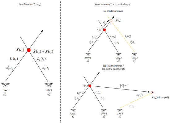
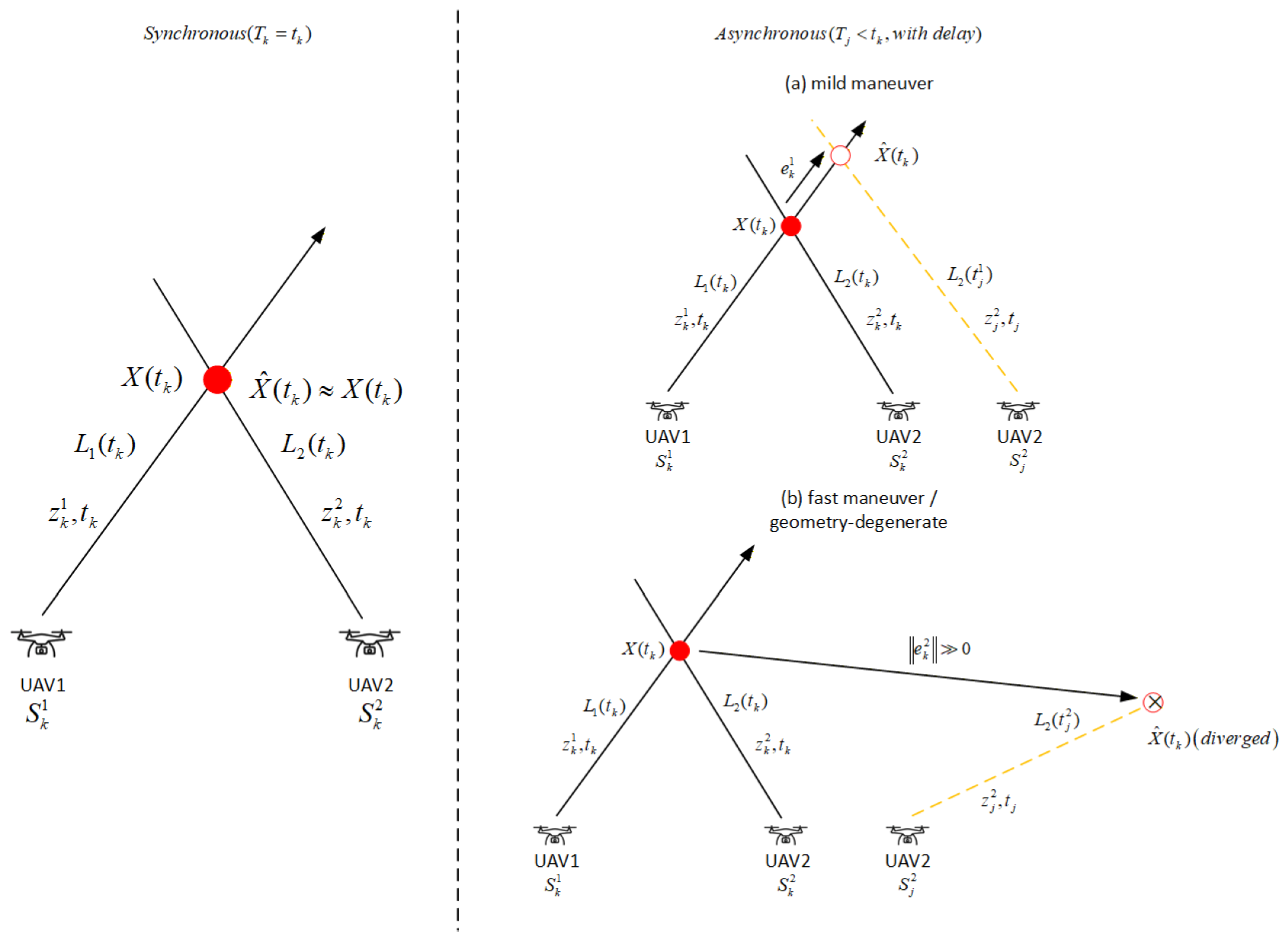
Figure 1 illustrates this geometric mismatch. In the synchronous scenario, the observation lines $L_1\left(t_k\right)$ and $L_2\left(t_k\right)$ of the local and remote platforms intersect at the same physical instant, and the state estimate satisfies $\widehat{\mathbf{X}}\left(t_k\right)\approx \mathbf{X}\left(t_k\right)$. In the asynchronous scenario, the historical remote ray $L_2\left(t_j\right)$ and the current local ray $L_1\left(t_k\right)$ are combined, and the intersection no longer corresponds to the current target state. When target maneuvering is mild, this mismatch mainly appears as a bounded bias; when the target maneuvers rapidly or the dual-UAV geometry degenerates, the error can be amplified, i.e., $\parallel e_k\parallel \gg 0$, and may cause filter divergence.

Figure 1. Geometric mechanism of synchronous and asynchronous bearing-only cooperative localization with delay. Subplot (a) represents the mild-maneuver scenario, and subplot (b) corresponds to fast maneuver or geometry-degenerate condition. The red solid dot denotes the true target state, the hollow circle is the filter estimate, the cross represents the diverged estimate, and yellow dashed lines indicate delayed historical measurement rays.

The above problem is especially prominent in angle-only cooperative localization. On the one hand, angle-only intersection requires the target position to be indirectly inferred through nonlinear geometric mapping, and high-speed relative platform motion amplifies the effect of measurement error. On the other hand, traditional analytical multistep OOSM update algorithms often require linearized approximations or equivalent state transformations when handling out-of-sequence data, which may introduce model errors. The problem addressed in this article is therefore how to exploit the timestamp and generation-time geometry of a late remote measurement while maintaining the availability of the current online estimate.

To address this problem, this article constructs two delayed remote-measurement compensation algorithms within a unified CKF recursion. The PCS algorithm performs predictive compensation in the current-state update through historical remote-innovation migration and covariance inflation; the TSA algorithm reconstructs the bistatic observation geometry at the generation time and propagates the correction forward in closed loop through finite-window historical replay. When the remote measurement is unavailable because of link factors, both algorithms degenerate to the single-station update that uses only the local measurement ${\mathbf{z}}_k^1$.

3. Delayed-Measurement Processing Methods and Communication- Disturbance Response Evaluation

This section first introduces the remote-measurement packet fields and the spatiotemporally decoupled cache-recording mechanism, and then presents the detailed implementation of two compensation algorithms under CKF recursion. The PCS algorithm corresponds to the Predictive Compensation Strategy; it uses historical innovation migration and covariance inflation to mitigate asynchronous fusion errors caused by late measurements in the current-state update. The TSA algorithm corresponds to the timestamp-alignment strategy; it reconstructs the bistatic observation geometry at the generation time through finite-window replay and then propagates the correction forward in closed loop. This section also defines the communication-disturbance response evaluation framework, where B characterizes the terminal-window localization error under the baseline communication link, and S, J, and L form the communication-disturbance response vector used in the partial-order relation and composite score.

3.1. Communication-Uncertainty Modeling and Spatiotemporally Decoupled Cache Records

3.1.1. Communication Delay Modeling

To describe random delay and its fluctuation, this article adopts nonnegative Gaussian sampling:

$$\tilde{\tau }\sim \mathcal{N}({\mu }_{\tau },{\sigma }_{\tau }^2),\tau =\max (0,\tilde{\tau }).$$

(40)

Here, $\tilde{\tau }$ is a Gaussian random variable, ${\mu }_{\tau }$ is the mean-delay parameter, ${\sigma }_{\tau }$ is the delay-standard-deviation parameter, and $\tau$ is the nonnegative communication delay actually used in the simulation. The variable $\tau$ has a discrete probability mass at zero,

$$P(\tau =0)=\mathrm{\Phi }\left(-{\displaystyle \frac{{\mu }_{\tau }}{{\sigma }_{\tau }}}\right),$$

(41)

and its cumulative distribution function can be written as

$$F_{\tau }\left(u\right)=P(\tau \le u)=\left\{\begin{array}{cc}0,\hfill & u<0,\hfill \\ \mathrm{\Phi }\left({\displaystyle \frac{u-{\mu }_{\tau }}{{\sigma }_{\tau }}}\right),\hfill & u\ge 0,\hfill \end{array}\right.$$

(42)

where $\mathrm{\Phi }(·)$ is the cumulative distribution function of the standard normal distribution.

3.1.2. Packet-Loss Modeling

Packet loss is modeled by the common Bernoulli model

$${\delta }_j\sim \mathrm{Bernoulli}\left(p_{\mathrm{loss}}\right),$$

(43)

where ${\delta }_j=1$ indicates that the jth remote packet is lost, ${\delta }_j=0$ indicates successful arrival, and $p_{\mathrm{loss}}$ is the packet-loss probability.

3.1.3. Data Packet Field Definition

The adopted communication model assigns one unique generation index j to each sampling instant and generates at most one remote packet at that instant. Each generated remote packet contains the timestamp $t_j$, bearing ${\mathbf{z}}_j^2={[{\alpha }_j^2,{\beta }_j^2]}^{\mathsf{T}}$, generation-time platform position ${\mathbf{S}}_j^2$, platform-velocity metadata ${\mathbf{v}}_j^2$, and arrival time $t_j^{\mathrm{arrival}}=t_j+{\tau }_j$ if it is not lost. These packet fields experience the same delay and loss event. In the reported filters, platform positions are treated as known geometric inputs; the velocity field is trajectory metadata and is not used as an additional measurement in the CKF update. Given the generation instant $t_j$, the probability that the packet arrives before fusion time t is

$$P\left(t_j^{\mathrm{arrival}}\le t\mid t_j\right)=\left\{\begin{array}{cc}(1-p_{\mathrm{loss}})F_{\tau }(t-t_j),\hfill & t\ge t_j,\hfill \\ 0,\hfill & t<t_j,\hfill \end{array}\right.$$

(44)

where $F_{\tau }(·)$ is the cumulative distribution function of the nonnegative communication-delay random variable $\tau$ defined above.

The simulation is performed at discrete sampling instants. Let the sampling period be $T_s$ and $t_k=k{T}_s$. The continuous arrival time is mapped to the earliest processable fusion instant as

$$a_j=\max \left(j,⌈{\displaystyle \frac{t_j^{\mathrm{arrival}}}{T_s}}⌉\right),d_j=a_j-j,$$

(45)

where $a_j$ is the discrete index at which the remote packet enters the fusion queue, and $d_j$ is the corresponding discrete delay in steps. If the jth packet is not lost and $a_j\le k$, it is available before time $t_k$. The arrival queue is ordered by $(t_j^{\mathrm{arrival}},j)$, and all packets released in the same fusion interval are processed in ascending generation-index order.

3.1.4. Spatiotemporally Decoupled Cache-Recording Mechanism

Under high-speed relative motion between the two platforms, the communication delay of remote measurements causes spatial geometry to become misaligned. To record the temporal and geometric information required by late measurements, this article constructs a spatiotemporally decoupled cache-recording mechanism. Let the effective traceback buffer length be $L_b$. At the current time k, the fusion node keeps only the index set within the effective historical window:

$${\mathcal{I}}_k=\{j:\max (0,k-L_b+1)\le j\le k\}.$$

(46)

For each time step, the historical cache snapshot is defined as

$$\begin{array}{cc}\hfill \mathcal{R}\left[k\right]& =\{{\mathbf{z}}_k^1,{\mathbf{R}}_k^1,{\mathbf{S}}_k^1,{\mathbf{z}}_k^2,{\mathbf{R}}_k^2,{\mathbf{S}}_k^2,{\chi }_k^2\},\hfill \\ \hfill \mathcal{X}\left[k\right]& =\{{\mathbf{x}}_{k|k-1},{\mathbf{P}}_{k|k-1},{\mathbf{x}}_{k|k},{\mathbf{P}}_{k|k}\},\hfill \end{array}$$

(47)

and the complete cache record is written as $\mathcal{B}\left[k\right]=\left\{\mathcal{R}\right[k],\mathcal{X}[k\left]\right\}$. Here, ${\mathbf{S}}_k^1$ and ${\mathbf{S}}_k^2$ record the synchronized bistatic geometry; ${\mathbf{R}}_k^1$ and ${\mathbf{R}}_k^2$ are the local and remote measurement covariances; and ${\chi }_k^2\in \{0,1\}$ indicates whether the remote measurement with timestamp k has become available. A generation-time record is initialized with a very large remote-noise variance, so the remote component contributes negligible information before arrival. When the corresponding packet arrives within the finite window, the record is activated by restoring the nominal remote-noise variance, and the flag remains active in later replays. When ${\chi }_k^2=0$, the update is therefore equivalent to a local-bearing-only update.

When an out-of-sequence packet with timestamp $t_j$ arrives, if $j\in {\mathcal{I}}_k$, the fusion node calls $\mathcal{B}\left[j\right]$ to recover the remote measurement noise and reconstruct the bistatic observation geometry at the generation time, which serves as the state entrance for filtering reconstruction in the TSA algorithm. If $j\notin {\mathcal{I}}_k$, the packet exceeds the traceback window and is discarded by the fusion node.

3.2. Delayed-Measurement Processing Algorithms

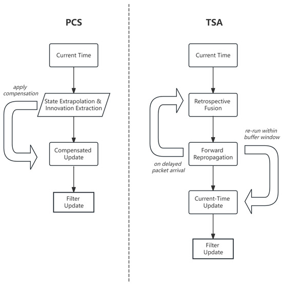
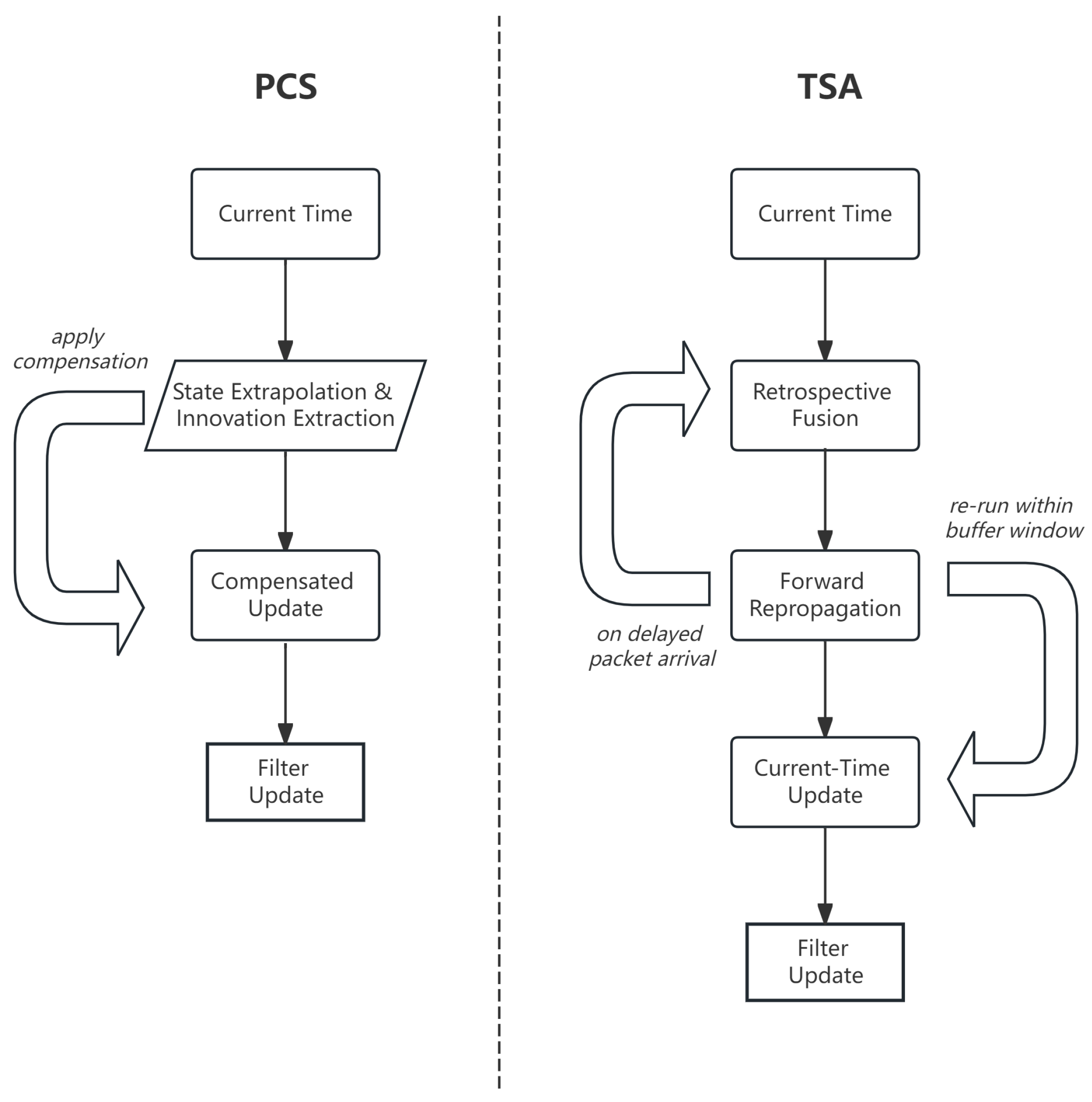
Based on the above mechanism, this article presents two delayed remote-measurement compensation algorithms, as summarized in Table 2 and illustrated in Figure 2. The PCS algorithm realizes predictive compensation in the current-state update through historical innovation migration and covariance inflation. The TSA algorithm performs Timestamp-Aligned Replay based on a finite historical window. The core difference between the two methods lies in whether historical replay is triggered when compensating a late measurement, and whether consistency between the measurement generation timestamp and observation geometry is restored at that historical instant.

Table 2. Timing characteristics of the two delayed-measurement compensation strategies.

Algorithm	Role	Delay Compensation	Historical Replay	Time Alignment
PCS	Predictive	Innovation migration; covariance inflation	No	Approximate
TSA	Finite-lag reprocessing	Generation-time activation; forward replay	Yes	Explicit

Figure 2. Comparison of the delayed-measurement compensation mechanisms of Predictive Compensation Strategy (PCS) and Timestamp-Aligned Replay (TSA).

3.2.1. PCS

PCS (Algorithm 1) does not replay historical filtering states. For a packet generated at $t_j$ and received at $t_k$, it computes the historical remote innovation

$${\mathit{\nu }}_j^2=\mathrm{wrap}\left[{\mathbf{z}}_j^2-h^2({\mathbf{x}}_j^L,{\mathbf{S}}_j^2)\right],{\rho }_j={\parallel {\mathit{\nu }}_j^2\parallel }_2,$$

(48)

where ${\mathbf{x}}_j^L$ is the cached local-only reference state. At the beginning of current-time remote processing, define

$$({\mathbf{x}}_k^{\left(0\right)},{\mathbf{P}}_k^{\left(0\right)})=({\mathbf{x}}_k^L,{\mathbf{P}}_k^L),$$

(49)

for an eligible packet with index j, let $\Delta t_j=t_k-t_j$. The migrated measurement is evaluated using the current remote-platform geometry ${\mathbf{S}}_k^2$, which is treated as a known input in the reported simulations. The innovation is accepted only if

$${\rho }_j\le {\rho }_{\max },$$

(50)

if packet $j_r$ is the rth packet that passes the optional age gate and the innovation gate in the current fusion interval, its innovation is transferred using the latest intermediate posterior:

$${\mathbf{z}}_{j_r\to k}^2=\mathrm{wrap}\left[h^2({\mathbf{x}}_k^{(r-1)},{\mathbf{S}}_k^2)+{\mathit{\nu }}_{j_r}^2\right],$$

(51)

PCS uses the following joint packet-age and innovation-magnitude covariance-inflation structure:

$$q(\Delta t,\rho )=1+c_t\Delta t+c_{tt}\Delta t^2+c_{\rho }{\left({\displaystyle \frac{\rho }{{\rho }_0}}\right)}^2,$$

(52)

where $c_t$, $c_{tt}$, and $c_{\rho }$ are inflation coefficients and ${\rho }_0$ is the innovation-normalization scale. Thus, ${\mathbf{R}}_{j_r\to k}^2=q(\Delta t_{j_r},{\rho }_{j_r}){\mathbf{R}}_{j_r}^2$. The remote-only CKF update maps $({\mathbf{x}}_k^{(r-1)},{\mathbf{P}}_k^{(r-1)})$ to $({\mathbf{x}}_k^{\left(r\right)},{\mathbf{P}}_k^{\left(r\right)})$; after all accepted packets have been processed, the last intermediate posterior becomes $({\mathbf{x}}_{k|k},{\mathbf{P}}_{k|k})$. This sequential notation matches the implemented processing procedure, in which the current intermediate state is updated after every accepted packet, and removes the ambiguity between a fixed local reference state and a state already corrected by an earlier packet in the same fusion interval. The function satisfies $q(0,0)=1$, $q\ge 1$, and is nondecreasing in both packet age and innovation magnitude. Because an angular residual depends on range, platform displacement, and target motion, this structure provides a reproducible low-cost mechanism for reducing the weight of older packets and larger migrated innovations. The numerical gate and inflation parameters used in the reported experiments are listed in Section 4.1.

Algorithm 1 PCS (Predictive Compensation Strategy: predictive compensation based on historical innovation migration and covariance inflation)

Require:  CKF operators $\mathcal{P}(·)$ and $\mathcal{U}(·)$; local measurement stream $\{{\mathbf{z}}_k^1,{\mathbf{R}}_k^1\}$; remote packets $\{t_j,{\mathbf{z}}_j^2,{\mathbf{R}}_j^2,{\mathbf{S}}_j^2\}$ and current remote-platform geometry ${\mathbf{S}}_k^2$; optional packet-age limit ${\tau }_{\max }\in (0,\infty ]$, innovation limit ${\rho }_{\max }$, and covariance-inflation function $q(\Delta t,\rho )$ Ensure:  Posterior estimates $\left\{({\mathbf{x}}_{k|k},{\mathbf{P}}_{k|k})\right\}$ 1: Initialize $({\mathbf{x}}_{0|0},{\mathbf{P}}_{0|0})$ and the local reference-trajectory cache $\left\{{\mathbf{x}}_k^L\right\}$ 2: for $k=1,2,\dots$ do 3:       Prediction: $({\mathbf{x}}_{k|k-1},{\mathbf{P}}_{k|k-1})\leftarrow \mathcal{P}({\mathbf{x}}_{k-1|k-1},{\mathbf{P}}_{k-1|k-1})$ 4:       Local baseline update: $({\mathbf{x}}_k^L,{\mathbf{P}}_k^L)\leftarrow \mathcal{U}({\mathbf{x}}_{k|k-1},{\mathbf{P}}_{k|k-1},{\mathbf{z}}_k^1,{\mathbf{R}}_k^1;h^1,{\mathbf{S}}_k^1)$ 5:       Set $r\leftarrow 0$ and $({\mathbf{x}}_k^{\left(0\right)},{\mathbf{P}}_k^{\left(0\right)})\leftarrow ({\mathbf{x}}_k^L,{\mathbf{P}}_k^L)$ 6:       for all unconsumed remote packets released at $t_k$, ordered by increasing j do 7:             if $t_k-t_j>{\tau }_{\max }$ then 8:                  Discard the packet and continue 9:             end if 10:           Compute historical innovation: ${\mathit{\nu }}_j^2\leftarrow \mathrm{wrap}({\mathbf{z}}_j^2-h^2({\mathbf{x}}_j^L,{\mathbf{S}}_j^2))$ 11:           if $\parallel {\mathit{\nu }}_j^2\parallel >{\rho }_{\max }$ then 12:                Discard this packet 13:           else 14:                Set $r\leftarrow r+1$ and $\Delta t_j\leftarrow t_k-t_j$ 15:                Migrate innovation: ${\mathbf{z}}_{j\to k}^2\leftarrow \mathrm{wrap}(h^2({\mathbf{x}}_k^{(r-1)},{\mathbf{S}}_k^2)+{\mathit{\nu }}_j^2)$ 16:                Inflate covariance: ${\mathbf{R}}_{j\to k}^2\leftarrow q(\Delta t_j,\parallel {\mathit{\nu }}_j^2\parallel ){\mathbf{R}}_j^2$ 17:                Sequential remote update: $({\mathbf{x}}_k^{\left(r\right)},{\mathbf{P}}_k^{\left(r\right)})\leftarrow \mathcal{U}({\mathbf{x}}_k^{(r-1)},{\mathbf{P}}_k^{(r-1)},{\mathbf{z}}_{j\to k}^2,{\mathbf{R}}_{j\to k}^2;h^2,{\mathbf{S}}_k^2)$ 18:           end if 19:     end for 20:     Output $({\mathbf{x}}_{k|k},{\mathbf{P}}_{k|k})\leftarrow ({\mathbf{x}}_k^{\left(r\right)},{\mathbf{P}}_k^{\left(r\right)})$ 21: end for

3.2.2. TSA

TSA (Algorithm 2) denotes Timestamp-Aligned Replay. Each packet released within the retained window activates the unique historical record associated with its generation index, whereas packets outside the index window are discarded according to the expiration rule. If several packets with different generation indices arrive in one fusion interval, all corresponding records are activated before a single replay starts from the oldest newly valid index; the later records are then encountered at their own timestamps during that replay. Previously arrived remote measurements remain active through ${\chi }_t^2=1$, so later replays preserve the available historical information.

Algorithm 2 TSA (Timestamp-Aligned Replay with deterministic packet consumption)

Require:  CKF operators $\mathcal{P}(·)$ and $\mathcal{U}(·)$; historical buffer $\mathcal{B}$ with length $L_b$; local measurement stream $\{{\mathbf{z}}_k^1,{\mathbf{R}}_k^1,{\mathbf{S}}_k^1\}$; asynchronous remote packets $\{t_j,{\mathbf{z}}_j^2,{\mathbf{R}}_j^2,{\mathbf{S}}_j^2\}$ Ensure:  Timestamp-aligned posterior estimates $\left\{({\mathbf{x}}_{k|k},{\mathbf{P}}_{k|k})\right\}$ 1: Initialize $({\mathbf{x}}_{0|0},{\mathbf{P}}_{0|0})$ and clear the historical state cache $\mathcal{B}$ 2: for $k=1,2,\dots$ do   3:       (A) Current-time local path 4:       $({\mathbf{x}}_{k|k-1},{\mathbf{P}}_{k|k-1})\leftarrow \mathcal{P}({\mathbf{x}}_{k-1|k-1},{\mathbf{P}}_{k-1|k-1})$ 5:       $({\mathbf{x}}_{k|k},{\mathbf{P}}_{k|k})\leftarrow \mathcal{U}({\mathbf{x}}_{k|k-1},{\mathbf{P}}_{k|k-1},{\mathbf{z}}_k^1,{\mathbf{R}}_k^1;h^1,{\mathbf{S}}_k^1)$ 6:       Store local data, geometry, prediction, posterior, and ${\chi }_k^2\leftarrow 0$ in $\mathcal{B}\left[k\right]$   7:       (B) Release, order, and activate packets 8:       ${\mathcal{A}}_k\leftarrow$ all queued packets with arrival time not later than $t_k$ 9:       Sort ${\mathcal{A}}_k$ by increasing generation index j; set ${\mathcal{J}}_k\leftarrow ⌀$ 10:     for all $p=(t_j,{\mathbf{z}}_j^2,{\mathbf{R}}_j^2,{\mathbf{S}}_j^2)\in {\mathcal{A}}_k$ do 11:           if $j<k-L_b+1$ then 12:                Discard p 13:           else 14:                Activate the remote fields in $\mathcal{B}\left[j\right]$ by setting ${\chi }_j^2\leftarrow 1$ and restoring nominal remote covariance 15:                ${\mathcal{J}}_k\leftarrow {\mathcal{J}}_k\cup \left\{j\right\}$ 16:           end if 17:     end for   18:     (C) One replay from the oldest newly valid timestamp 19:     if ${\mathcal{J}}_k\ne ⌀$ then 20:           $j^{\star }\leftarrow \min {\mathcal{J}}_k$ and recover the posterior at $j^{\star }-1$ (or the initial prior if $j^{\star }=0$) 21:           for $t=j^{\star }$ to k do 22:                Predict $({\tilde{\mathbf{x}}}_{t|t-1},{\tilde{\mathbf{P}}}_{t|t-1})$ from the corrected posterior at $t-1$ 23:                if ${\chi }_t^2=1$ then 24:                      Update with $[{\mathbf{z}}_t^1;{\mathbf{z}}_t^2]$, ${\mathbf{R}}_{t,t}^{\mathrm{comb}}$, and $\{{\mathbf{S}}_t^1,{\mathbf{S}}_t^2\}$ 25:                else 26:                      Update with the local bearing ${\mathbf{z}}_t^1$ and ${\mathbf{S}}_t^1$ 27:                end if 28:                Write the new prediction and posterior to $\mathcal{B}\left[t\right]$ 29:           end for 30:     end if 31:     Output the current posterior already stored at $\mathcal{B}\left[k\right]$ 32: end for

For state dimension n, one CKF prediction/update has the usual matrix-factorization cost, denoted here by $C_{\mathrm{CKF}}\left(n\right)$. Current Direct Strategy(CDS) and PCS require $O\left(C_{\mathrm{CKF}}\left(n\right)\right)$ per ordinary fusion step, whereas TSA requires $O\left({\mathcal{l}}_k{C}_{\mathrm{CKF}}\left(n\right)\right)$ when a replay of length ${\mathcal{l}}_k\le L_b$ is triggered. Because all newly valid packets released in one interval are validated and activate their records before a single replay, the cost does not multiply by the number of arrivals in that interval. The cache stores $L_b$ state means, covariances, measurements, and geometry, giving $O\left(L_b{n}^2\right)$ numeric storage.

3.3. Communication-Disturbance Response Evaluation Framework

The evaluation framework jointly considers baseline localization accuracy and responses to average delay, delay jitter, and packet loss. The primary comparison uses the four-dimensional vector $(B,S,J,L)$ and Pareto dominance. A normalized weighted score is retained only as a secondary summary because it depends on the scan grid, candidate algorithms, and selected weights. Extreme packet-loss cases are reported as stress tests and are not used to fit L.

3.3.1. Evaluation Inputs and Baseline Error

Let the communication-link parameter vector and the baseline communication-link parameter vector be

$$\mathit{\eta }={[{\mu }_{\tau },{\sigma }_{\tau },p_{\mathrm{loss}}]}^{\mathrm{T}},{\mathit{\eta }}_0={[{\mu }_{\tau ,0},{\sigma }_{\tau ,0},p_0]}^{\mathrm{T}}.$$

(53)

Here, ${\mu }_{\tau }$ is the average delay, ${\sigma }_{\tau }$ is the delay standard deviation, and $p_{\mathrm{loss}}$ is the packet-loss rate. Let ${ϵ}_{\pi ,\mathrm{term}}\left(\mathit{\eta }\right)$ denote the terminal-window mean sample-wise three-axis root-mean-square(RMS) position error defined in Section 4. The baseline metric is

$$B_{\pi }={ϵ}_{\pi ,\mathrm{term}}\left({\mathit{\eta }}_0\right).$$

(54)

3.3.2. Average Delay Sensitivity

In the average-delay scan, the path is defined as

$${\mathcal{C}}_{\tau }=\{(\tau ,g_{\tau }\left(\tau \right),p_0):\tau \in [{\tau }_{\min },{\tau }_{\max }]\},$$

(55)

where ${\tau }_{\min }$ and ${\tau }_{\max }$ denote the lower and upper bounds of the average-delay scan, respectively, and $g_{\tau }(·)$ is the path function that specifies the associated delay jitter during the average-delay scan. The average-delay sensitivity is defined as

$$\begin{array}{cc}\hfill S_{\pi }& ={\displaystyle \frac{1}{N_{\tau }-1}}{\displaystyle \sum _{i=1}^{N_{\tau }-1}}\left|{\displaystyle \frac{{\Delta }_{\tau ,i}^{\pi }}{{\tau }_{i+1}-{\tau }_i}}\right|,\hfill \\ \hfill {\Delta }_{\tau ,i}^{\pi }& ={ϵ}_{\pi ,\mathrm{term}}({\tau }_{i+1},g_{\tau }\left({\tau }_{i+1}\right),p_0)\hfill \\ \hfill & -{ϵ}_{\pi ,\mathrm{term}}({\tau }_i,g_{\tau }\left({\tau }_i\right),p_0).\hfill \end{array}$$

(56)

where $N_{\tau }$ is the number of average-delay scan points. In addition to the absolute-slope measure $S_{\pi }$, the signed endpoint slope $D_{\tau ,\pi }=[{ϵ}_{\pi ,\mathrm{term}}\left({\tau }_{N_{\tau }}\right)-{ϵ}_{\pi ,\mathrm{term}}\left({\tau }_1\right)]/({\tau }_{N_{\tau }}-{\tau }_1)$ is reported to distinguish net degradation from nonmonotone scan noise.

3.3.3. Delay-Jitter Sensitivity

In the jitter scan, the delay-jitter sensitivity is defined as

$$\begin{array}{cc}\hfill J_{\pi }& ={\displaystyle \frac{1}{N_{\sigma }-1}}{\displaystyle \sum _{i=1}^{N_{\sigma }-1}}\left|{\displaystyle \frac{{\Delta }_{\sigma ,i}^{\pi }}{{\sigma }_{i+1}-{\sigma }_i}}\right|,\hfill \\ \hfill {\Delta }_{\sigma ,i}^{\pi }& ={ϵ}_{\pi ,\mathrm{term}}({\mu }_{\tau ,0},{\sigma }_{i+1},p_0)\hfill \\ \hfill & -{ϵ}_{\pi ,\mathrm{term}}({\mu }_{\tau ,0},{\sigma }_i,p_0).\hfill \end{array}$$

(57)

where $N_{\sigma }$ is the number of delay-jitter scan points. The corresponding signed endpoint slope $D_{\sigma ,\pi }$ is reported alongside $J_{\pi }$.

3.3.4. Packet-Loss Response Intensity

In the packet-loss scan, the complete set of scan points ${\mathcal{P}}_{\mathrm{all}}$ consists of the discrete points in the main evaluation interval ${\mathcal{P}}_{\mathrm{main}}$ and the stress-test points ${\mathcal{P}}_{\mathrm{stress}}$. The set ${\mathcal{P}}_{\mathrm{main}}$ is used to compute $L_{\pi }$, whereas ${\mathcal{P}}_{\mathrm{stress}}$ is used only to illustrate extended trends and is not included in the partial-order comparison or the composite score. The scan points are given in Section 4. Let

$${ϵ}_{\pi ,\mathrm{term}}^{\left(p\right)}\left(p\right)={ϵ}_{\pi ,\mathrm{term}}({\mu }_{\tau ,0},{\sigma }_{\tau ,0},p),$$

(58)

and fit it with a first-order model over ${\mathcal{P}}_{\mathrm{main}}$ in the main evaluation interval as

$${ϵ}_{\pi ,\mathrm{term}}^{\left(p\right)}\left(p\right)\approx a_{\pi }+b_{\pi }p.$$

(59)

Here, $a_{\pi }$ and $b_{\pi }$ are the fitted intercept and slope of algorithm $\pi$, respectively. Since p is expressed in decimal form, $b_{\pi }$ represents the error variation rate when the packet-loss rate increases from 0 to 1. On this basis, the normalized packet-loss response intensity is defined as

$$L_{\pi }={\displaystyle \frac{|b_{\pi }|}{{ϵ}_{\pi ,\mathrm{term}}({\mu }_{\tau ,0},{\sigma }_{\tau ,0},0)}}.$$

(60)

This definition uses the absolute slope to characterize the magnitude of the error variation with packet-loss rate in the main evaluation interval. Because random loss of remote packets changes the temporal combination by which delayed measurements enter the filter, local errors need not vary strictly monotonically with the packet-loss rate. Therefore, this article uses the absolute normalized fitted slope $L_{\pi }$ over the main evaluation interval to characterize the packet-loss response intensity.

3.3.5. Communication-Disturbance Response Vector and Composite Evaluation

The primary accuracy–response vector is

$${\mathbf{\Phi }}_{\pi }={[B_{\pi },S_{\pi },J_{\pi },L_{\pi }]}^{\mathrm{T}}.$$

(61)

For any two algorithms ${\pi }_a$ and ${\pi }_b$, if

$${\mathbf{\Phi }}_{{\pi }_a}\le {\mathbf{\Phi }}_{{\pi }_b}$$

(62)

and at least one dimension is strictly smaller, then ${\pi }_a$ Pareto-dominates ${\pi }_b$. For each metric $X\in \{B,S,J,L\}$, min–max normalization is

$${\tilde{X}}_{\pi }={\displaystyle \frac{X_{\pi }-{\min }_j{X}_j}{{\max }_j{X}_j-{\min }_j{X}_j}},$$

(63)

and the secondary four-dimensional score is

$${\mathrm{\Gamma }}_{\pi }^{\mathrm{BSJL}}=w_B{\tilde{B}}_{\pi }+w_S{\tilde{S}}_{\pi }+w_J{\tilde{J}}_{\pi }+w_L{\tilde{L}}_{\pi },$$

(64)

where the nonnegative weights satisfy $w_B+w_S+w_J+w_L=1$. Because min–max values change when a candidate algorithm is added, ${\mathrm{\Gamma }}^{\mathrm{BSJL}}$ is retained only as a secondary summary. The Pareto relation and the unnormalized B, S, J, and L metrics remain the primary evidence. The numerical weights used for the reported secondary score are listed in Section 4.1.

3.4. Dimensional Response Mechanism Analysis

The strategies differ mainly in how they handle time and geometry when a delayed measurement enters the filter. Suppose that a remote packet is generated at $t_j$ and arrives at $t_k$ ($j\le k$), and denote the time difference by ${\Delta }_{j,k}=t_k-t_j$. By applying a first-order Taylor expansion to the remote nonlinear observation function $h^2(\mathbf{X},{\mathbf{S}}^2)$ at the current operating point, the residual offset caused by the absence of spatiotemporal alignment can be approximated as

$$\delta {\mathbf{r}}_{j\to k}\approx {\mathbf{H}}_{X,k}^2({\mathbf{X}}_j-{\mathbf{X}}_k)+{\mathbf{H}}_{S,k}^2({\mathbf{S}}_j^2-{\mathbf{S}}_k^2)+\Delta {\mathbf{w}}_{j,k}^2,$$

(65)

where ${\mathbf{H}}_{X,k}^2$ and ${\mathbf{H}}_{S,k}^2$ denote the Jacobian matrices of the remote bearing observation with respect to the target motion state and the spatial evolution of the observing platform, respectively, and $\Delta {\mathbf{w}}_{j,k}^2$ denotes the disturbance term introduced by the delay difference. This equation shows that temporal mismatch simultaneously produces target-state extrapolation deviation and platform-observation-geometry displacement error. The multidimensional metrics defined above are intended to observe the responses of these error sources under different communication conditions.

Without temporal intervention, the delayed measurement in the currently available queue is directly incorporated into the filter update at $t_k$. According to Equation (65), the deviation term caused by target maneuvering and the platform-geometry misalignment term directly enter the residual calculation. As the target maneuver intensity increases or the average delay becomes longer, the estimation bias is more likely to grow. Therefore, the uncompensated direct-fusion result is used to characterize the baseline error when no spatiotemporal alignment is applied.

Compared with direct fusion, PCS introduces a locally extrapolated trajectory, extracts the historical innovation, and performs the current-state compensation update after covariance inflation. This procedure can reduce the direct effect of delayed measurements on the current gain calculation. However, PCS depends on the accuracy of the locally extrapolated trajectory ${\mathbf{x}}_j^L$. When the target undergoes strong maneuvers or the delay jitter becomes severe, single-station extrapolation errors affect innovation migration, which may lead to higher sensitivity in the jitter-resistance metric J. Meanwhile, the compensation gain of PCS comes from historical innovations provided by arriving remote packets. Packet loss reduces compensation opportunities and increases the proportion of single-station extrapolation; hence, L can be used to observe its sensitivity to variations in the availability of remote packets.

The TSA approach restores the observation geometry at the generation time. Instead of forcibly transforming historical remote measurements into current compensation measurements, it rolls delayed measurements back to the historical node $t_j$. With the aid of cached records, the bistatic observation residual at $t_j$ is reconstructed as

$${\mathbf{r}}_j^{\mathrm{TSA}}={\mathbf{Z}}_j^{\mathrm{comb}}-h({\mathbf{x}}_{j|j-1},{\mathbf{S}}_j^1,{\mathbf{S}}_j^2).$$

(66)

Because the measurement timestamp and platform geometry are made consistent again, TSA can reduce offset terms introduced by analytical approximation or by forced conversion into current compensation measurements. Its cost is that historical states must be propagated forward in closed loop within a finite window. Nevertheless, each successfully arriving delayed remote packet acts under the nonlinear observation geometry of its corresponding timestamp, yielding high utilization efficiency for each remote packet. Therefore, when the packet-loss rate varies within the main evaluation interval, the terminal-window error of TSA is usually not significantly amplified by a small number of lost packets, and it maintains low error levels for both the baseline terminal-window error metric B and the communication-disturbance response metrics S, J, and L.

4. Numerical Simulations

This section evaluates delayed-measurement processing in dual-UAV cooperative passive localization through numerical simulations. The principal communication scans use 100 Monte Carlo trials. Unless otherwise stated, Monte Carlo results are reported as mean ± empirical standard deviation. Additional comparisons examine reference algorithms, PCS parameters, TSA buffer length, computational cost, and bearing-noise sensitivity.

4.1. Simulation Setup

The scenario parameters and reported trajectories use a north-east-down (NED) coordinate system. The initial UAV positions and their common velocity are

$$\begin{array}{cccc}\hfill {\mathbf{S}}_0^1& ={[\mathrm{70,000},-\mathrm{20,000},-6000]}^{\mathrm{T}}\mathrm{m},\hfill & \hfill {\mathbf{S}}_0^2& ={[\mathrm{80,000},-\mathrm{10,000},-7000]}^{\mathrm{T}}\mathrm{m},\hfill \\ \hfill {\mathbf{v}}_{\mathrm{UAV},1}& ={\mathbf{v}}_{\mathrm{UAV},2}={[-238.20,-238.20,0.00]}^{\mathrm{T}}\mathrm{m}/\mathrm{s}.\hfill & & \end{array}$$

The target initial position and velocity are

$${\mathbf{p}}_0^{\mathrm{T}}=[\mathrm{45,000},-\mathrm{80,000},-8000]\mathrm{m},{\mathbf{v}}_0^{\mathrm{T}}=[238.20,170.15,-1.70]\mathrm{m}/\mathrm{s}.$$

The corresponding true initial state is

$${\mathbf{X}}_0^{\mathrm{true}}={[\mathrm{45,000},238.20,0,-\mathrm{80,000},170.15,0,-8000,-1.70,0,0]}^{\mathrm{T}}.$$

(67)

Each Monte Carlo trial uses

$${\widehat{\mathbf{X}}}_0={\mathbf{X}}_0^{\mathrm{true}}+{ϵ}_0,$$

(68)

where

$${ϵ}_0\sim \mathcal{N}\left(\mathbf{0},\mathrm{diag}({100}^2,{10}^2,{0.5}^2,{100}^2,{10}^2,{0.5}^2,{50}^2,5^2,{0.2}^2,{10}^{-6})\right),$$

(69)

and the initial covariance is

$${\mathbf{P}}_0=\mathrm{diag}({10}^4,{10}^2,10,{10}^4,{10}^2,10,{10}^2,10,10,4\times {10}^{-4}).$$

(70)

All compared algorithms use the same initialization distribution and covariance.

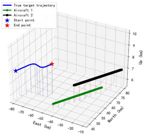
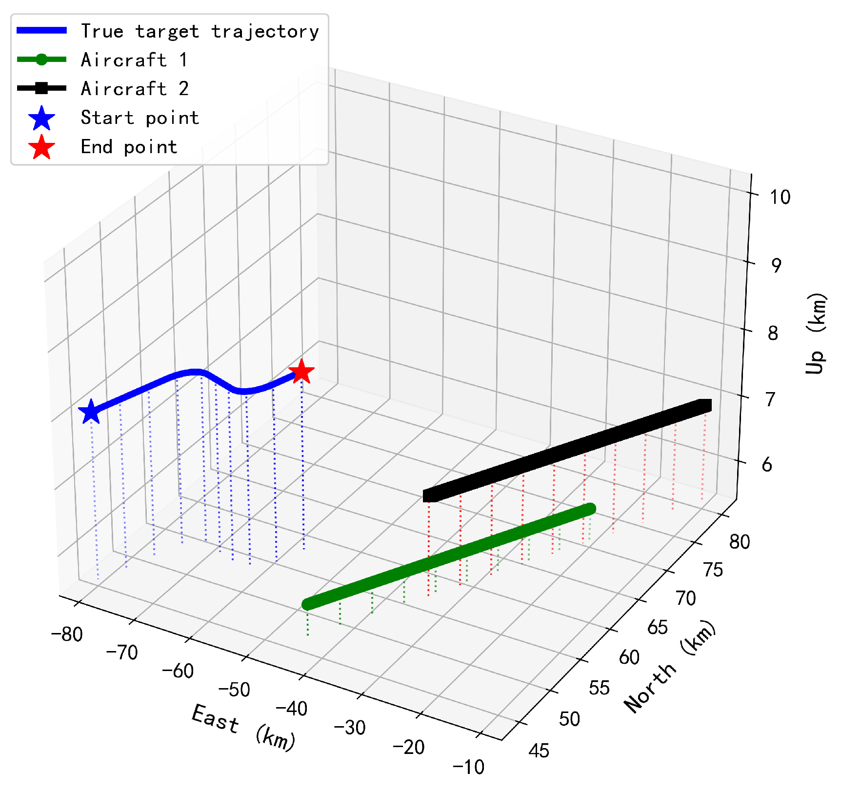
The target moves in uniform straight motion during 1–$29\mathrm{s}$, 49–$69\mathrm{s}$, and 89–$100\mathrm{s}$, and performs horizontal turns of radius $5\mathrm{km}$ during the remaining intervals. The total duration is $100\mathrm{s}$. The filter estimates three-dimensional position; the tested target maneuvers mainly in the horizontal plane, while its vertical velocity remains approximately constant. Figure 3 shows the scenario in the NED frame.

Figure 3. Three-dimensional trajectories of the dual UAVs and target, with auxiliary projection drop lines.

The state-propagation and fusion sampling intervals are identical, $T=T_s=50\mathrm{ms}$. The azimuth and elevation measurement-noise standard deviations are both $1.8\mathrm{mrad}$, and the turn-rate estimation standard deviation inherited from the reference model is set to ${\sigma }_{\omega }=10\mathrm{mrad}/\mathrm{s}={10}^{-2}\mathrm{rad}/\mathrm{s}$. The simulations treat UAV positions as deterministic known inputs; platform-position and attitude uncertainty are not propagated through the bearing model.

PCS uses no explicit maximum packet age in the principal communication scans and algorithm comparisons, while the innovation gate is

$${\tau }_{\max }^{\mathrm{PCS}}=\infty ,{\rho }_{\max }=0.12\mathrm{rad},$$

and the covariance-inflation structure defined in Section 3 uses

$$c_t=4.0{\mathrm{s}}^{-1},c_{tt}=8.0{\mathrm{s}}^{-2},c_{\rho }=1.5,{\rho }_0=\max (8{\sigma }_{\theta },0.02\mathrm{rad})=0.02\mathrm{rad}.$$

These coefficients were selected heuristically before the communication scans and were then held fixed in all principal PCS comparisons; they were not optimized separately at each communication condition.

When $|{\omega }_k|<{10}^{-9}\mathrm{rad}/\mathrm{s}$, the turn-rate-dependent fractions in the state transition and process covariance are evaluated using the zero-turn-rate continuous limits given in Section 2.

The historical buffer length of the TSA algorithm is fixed at $L_b=40$ stored nodes. Under the sampling interval $T_s=50\mathrm{ms}$, the nominal storage duration is $L_b{T}_s=2.0\mathrm{s}$, whereas the actual time difference between the earliest and current stored indices is

$$T_{\mathrm{span}}=(L_b-1)T_s=39\times 0.05=1.95\mathrm{s}.$$

Under $({\mu }_{\tau ,0},{\sigma }_{\tau ,0})=(1.0\mathrm{s},0.3\mathrm{s})$, this span exceeds ${\mu }_{\tau ,0}+3{\sigma }_{\tau ,0}=1.9\mathrm{s}$ and covers the principal range of the baseline delay distribution. CDS imposes no explicit packet-age cutoff and directly incorporates the remote packet selected from the arrived queue at the current fusion time. PCS likewise has no hard packet-age cutoff; instead, its delay-dependent covariance inflation progressively reduces the weight of older packets, while the innovation gate rejects unusually large residuals. TSA can replay only timestamps retained in its 40-node cache, which provides an effective maximum lag of $1.95\mathrm{s}$, and packets outside that window are discarded. The principal comparisons use these fixed packet-handling rules for the respective strategies.

The principal communication scans compare CDS, PCS, and TSA. The six-strategy jitter comparison also includes Local, which uses only UAV 1; Age-Limited Direct, which fuses the newest arrived remote packet within the packet-age limit without replay; and OOSM-CKF, which applies a delayed-time update followed by prediction and current-time fusion.

In the communication-disturbance response evaluation, the baseline communication-link parameter vector is set as

$${\mathit{\eta }}_0={[1.0\mathrm{s},0.3\mathrm{s},5\%]}^{\mathrm{T}}.$$

The average-delay scan uses $g_{\tau }\left(\tau \right)=\max (0.1,\tau /3)$ with fixed $p_0=5\%$. The delay-jitter scan fixes ${\mu }_{\tau ,0}=1.0\mathrm{s}$ and $p_0=5\%$, and the packet-loss scan fixes ${\mu }_{\tau ,0}=1.0\mathrm{s}$ and ${\sigma }_{\tau ,0}=0.3\mathrm{s}$. The complete packet-loss scan set is displayed in percentages in the figures and tables and converted to decimal form during metric calculation:

$${\mathcal{P}}_{\mathrm{all}}=\{0,5,10,15,20,40,60,80\}\%,$$

where ${\mathcal{P}}_{\mathrm{main}}=\{0,5,10,15,20\}\%$ denotes the fitting interval and ${\mathcal{P}}_{\mathrm{stress}}=\{40,60,80\}\%$ denotes stress-test points.

The secondary normalized BSJL score uses

$$(w_B,w_S,w_J,w_L)=(0.35,0.25,0.20,0.20),$$

while the unnormalized response vector and Pareto relation remain the primary comparison criteria.

4.2. Performance Metrics

For trial i and time k, the sample-wise three-axis RMS position error is defined as

$$e_{\pi }^{\left(i\right)}(k;\mathit{\eta })=\sqrt{{\displaystyle \frac{{(x_k-{\widehat{x}}_{\pi ,k}^{\left(i\right)})}^2+{(y_k-{\widehat{y}}_{\pi ,k}^{\left(i\right)})}^2+{(z_k-{\widehat{z}}_{\pi ,k}^{\left(i\right)})}^2}{3}}}.$$

(71)

For a time-index set $\mathcal{K}$, the trial-level mean sample-wise three-axis RMS position error is

$${ϵ}_{\pi }^{\left(i\right)}(\mathcal{K};\mathit{\eta })={\displaystyle \frac{1}{\left|\mathcal{K}\right|}}\sum _{k\in \mathcal{K}}{e}_{\pi }^{\left(i\right)}(k;\mathit{\eta }).$$

(72)

The reported Monte Carlo mean and empirical standard deviation are then calculated from these trial-level values:

$$\begin{array}{cc}\hfill {ϵ}_{\pi }(\mathcal{K};\mathit{\eta })& ={\displaystyle \frac{1}{N_{\mathrm{MC}}}}{\displaystyle \sum _{i=1}^{N_{\mathrm{MC}}}}{ϵ}_{\pi }^{\left(i\right)}(\mathcal{K};\mathit{\eta }),\hfill \\ \hfill s_{\pi }(\mathcal{K};\mathit{\eta })& =\sqrt{{\displaystyle \frac{1}{N_{\mathrm{MC}}-1}}\sum _{i=1}^{N_{\mathrm{MC}}}{\left[{ϵ}_{\pi }^{\left(i\right)}(\mathcal{K};\mathit{\eta })-{ϵ}_{\pi }(\mathcal{K};\mathit{\eta })\right]}^2}.\hfill \end{array}$$

(73)

The full-trajectory set is ${\mathcal{K}}_{\mathrm{all}}=\{1,\dots ,K\}$, the maneuver-only set contains 29–$49\mathrm{s}$ and 69–$89\mathrm{s}$, and

$${\mathcal{K}}_{\mathrm{term}}=\{k:k\ge 0.8K\},{ϵ}_{\pi ,\mathrm{term}}\left(\mathit{\eta }\right)={ϵ}_{\pi }({\mathcal{K}}_{\mathrm{term}};\mathit{\eta }).$$

(74)

The quantity in the preceding equations is a mean of already square-rooted sample-wise values. It is therefore not the conventional trajectory-level position RMSE, which averages squared position errors before applying a final square root. Here, ${ϵ}_{\pi }$ is termed the mean sample-wise three-axis RMS position error. All position-error figures and tables in the baseline comparison, principal communication scans, PCS structure ablation, and extended comparisons use this definition.

Because 80–$100\mathrm{s}$ includes a turn until $89\mathrm{s}$ and straight motion thereafter, ${ϵ}_{\pi ,\mathrm{term}}$ is interpreted as a terminal-window mean sample-wise three-axis RMS position error rather than a strict steady-state quantity.

4.3. Performance Analysis and Communication-Disturbance Response Evaluation Results

4.3.1. Terminal-Window Mean Sample-Wise Three-Axis RMS Position Error Under the Baseline Communication Link (B)

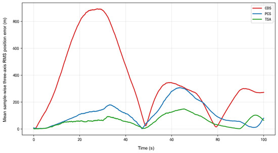
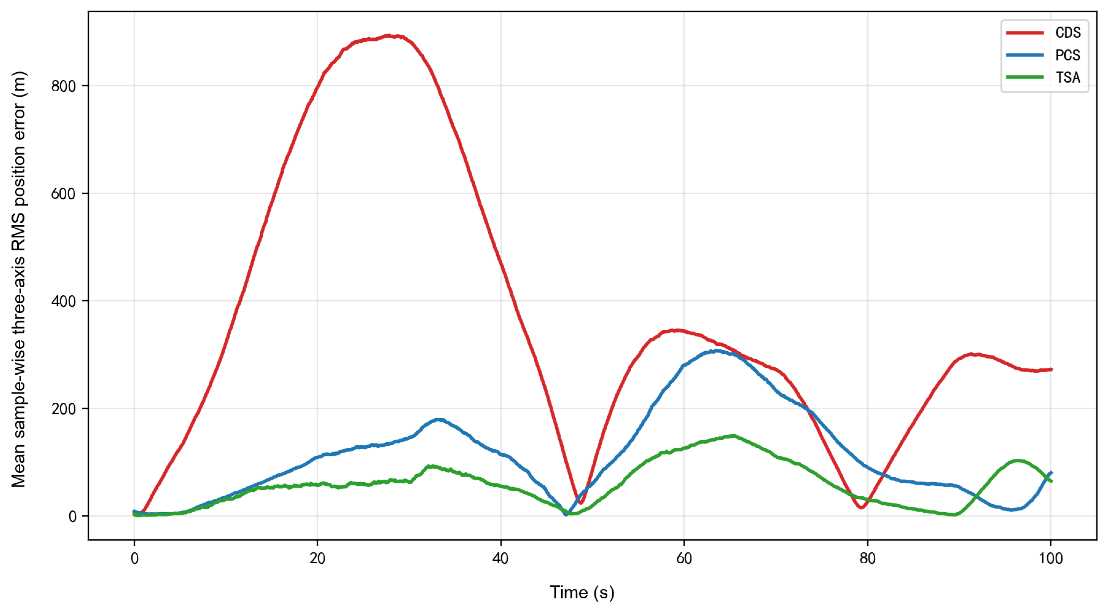
Under the baseline link, the terminal-window mean sample-wise three-axis RMS position error B is $226.70\mathrm{m}$ for CDS, $48.86\mathrm{m}$ for PCS, and $42.45\mathrm{m}$ for TSA. PCS and TSA therefore reduce this error by $78.4\%$ and $81.3\%$, respectively, relative to direct fusion. TSA achieves the lowest terminal-window mean sample-wise three-axis RMS position error. Figure 4 reports the mean sample-wise three-axis RMS position error at each time instant.

Figure 4. Time histories of the mean sample-wise three-axis root-mean-square(RMS) position error under the baseline communication link (${\mu }_{\tau }=1.0\mathrm{s},{\sigma }_{\tau }=0.3\mathrm{s},p_{\mathrm{loss}}=5\%$).

Table 3 reports B, the terminal-window mean sample-wise three-axis RMS position error, for the baseline comparison. The subsequent communication-scan tables report the mean and empirical standard deviation of the same terminal-window error metric.

Table 3. Terminal-window mean sample-wise three-axis RMS position error under the baseline communication link.

Algorithm	B: Terminal-Window Mean Error (m)	Reduction vs. CDS (%)
CDS	226.70	0.0
PCS	48.86	78.4
TSA	42.45	81.3

4.3.2. Average-Delay Sensitivity (S)

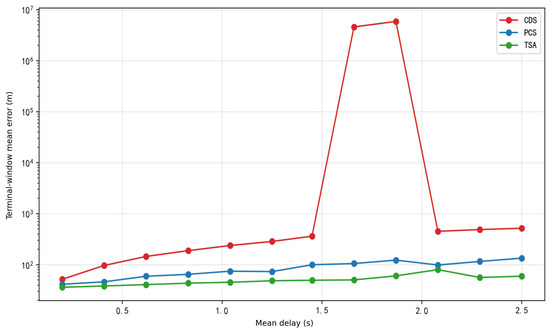
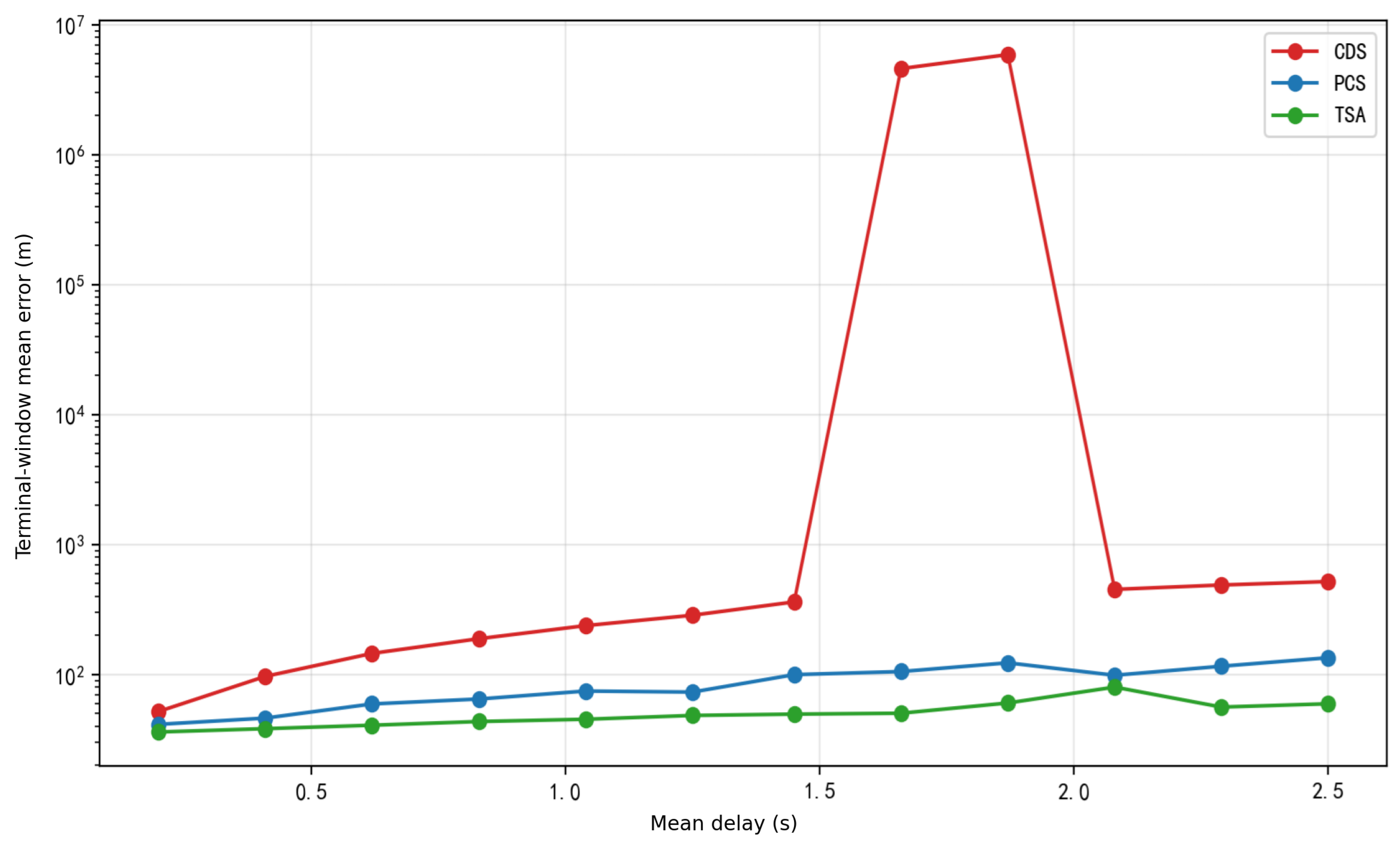
As shown in Figure 5 and Table 4, CDS develops a heavy-tailed failure region around ${\mu }_{\tau }=1.66$–$1.87\mathrm{s}$. At $1.66\mathrm{s}$, its mean terminal-window sample-wise three-axis RMS position error is $4.60\times {10}^6\mathrm{m}$ with a standard deviation of $4.60\times {10}^7\mathrm{m}$ over 100 trials, whereas adjacent non-failure cells are several hundred meters. The order-of-magnitude excess of the standard deviation over the mean shows that the cell is dominated by a small number of extreme trajectories; consequently, the raw mean and the derived $S=5.11\times {10}^6\mathrm{m}/\mathrm{s}$ must be interpreted together with the reported dispersion. PCS and TSA remain below $136\mathrm{m}$ at the displayed points. Their signed endpoint slopes are $40.60\mathrm{m}/\mathrm{s}$ and $10.20\mathrm{m}/\mathrm{s}$, respectively, compared with $203.26\mathrm{m}/\mathrm{s}$ for CDS when only the endpoints are used. This signed diagnostic and the four-dimensional Pareto comparison reduce reliance on the single unstable cell. Figure 5 use the y-axis term “Terminal-window mean error” for ${ϵ}_{\pi ,\mathrm{term}}$, i.e., the mean of the sample-wise three-axis RMS position error over 80–$100\mathrm{s}$ and all Monte Carlo trials.

Figure 5. Terminal-window mean error under the average-delay scan (${\sigma }_{\tau }=\max (0.1,{\mu }_{\tau }/3)$, $p_{\mathrm{loss}}=5\%$).

Table 4. Terminal-window mean sample-wise three-axis RMS position error under different average delays.

Mean Delay ${\mathit{\mu }}_{\mathit{\tau }}$ (s)	CDS Terminal-Window Error Mean ± std (m)	PCS Terminal-Window Error Mean ± std (m)	TSA Terminal-Window Error Mean ± std (m)
0.20	$51.88\pm 17.21$	$41.34\pm 27.90$	$36.12\pm 6.91$
1.04	$237.87\pm 18.64$	$74.63\pm 64.05$	$45.27\pm 6.59$
1.66	$(4.60\pm 46.02)\times {10}^6$	$105.42\pm 115.83$	$50.37\pm 9.06$
2.08	$452.12\pm 106.70$	$98.71\pm 118.19$	$80.06\pm 194.69$
2.50	$519.37\pm 63.47$	$134.73\pm 144.88$	$59.57\pm 22.40$

4.3.3. Delay-Jitter Sensitivity (J)

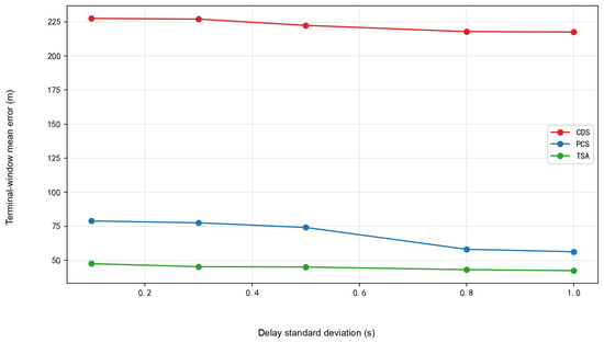
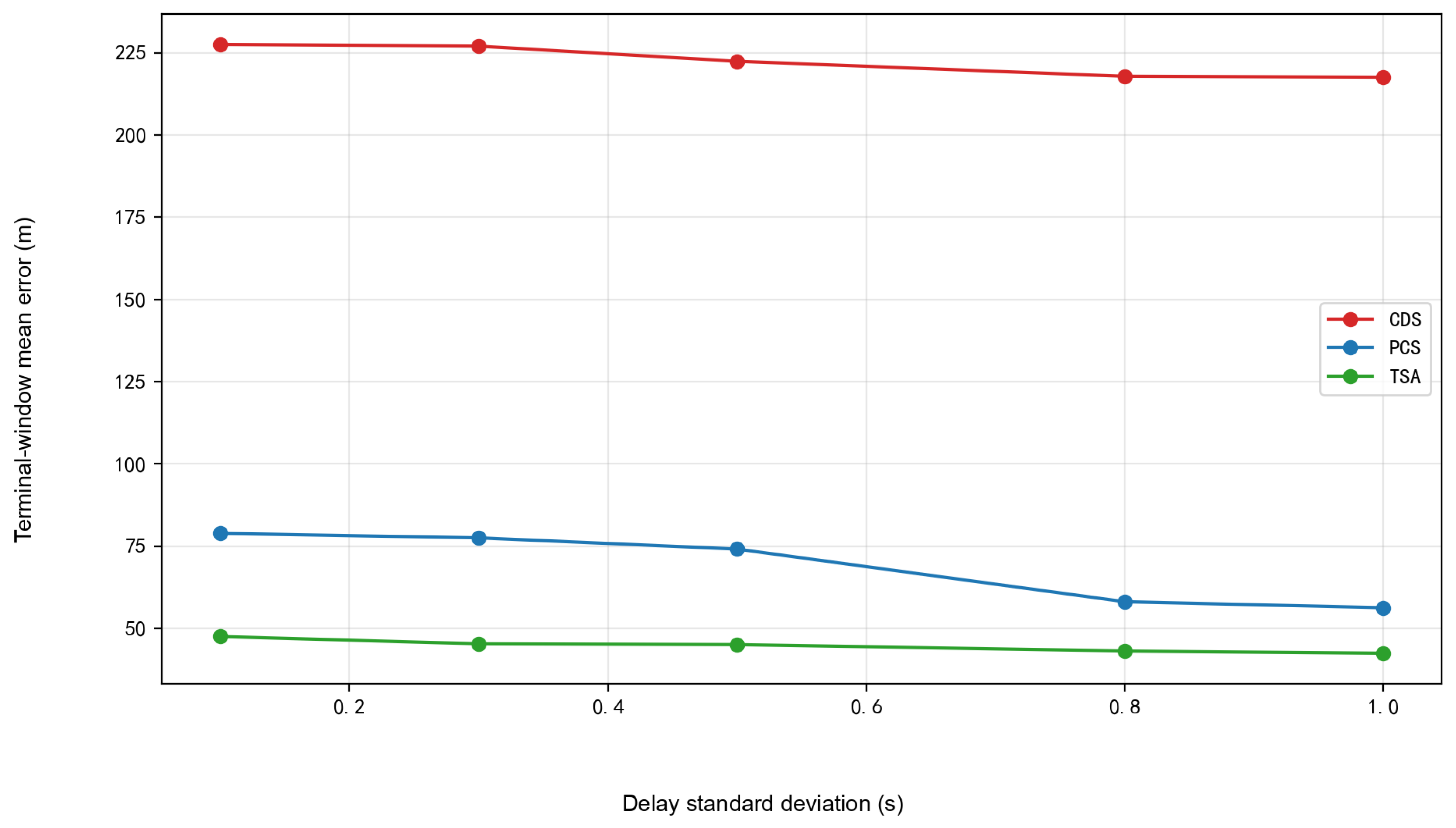
The delay-jitter sensitivity J characterizes the total adjacent-point variation in the terminal-window mean sample-wise three-axis RMS position error. Figure 6 and Table 5 report the error trend and pointwise statistics, respectively. Figure 6 use the y-axis term “Terminal-window mean error” for ${ϵ}_{\pi ,\mathrm{term}}$, i.e., the mean of the sample-wise three-axis RMS position error over 80–$100\mathrm{s}$ and all Monte Carlo trials. CDS remains at a high error level of about 217–$228\mathrm{m}$; its relatively small $J=10.57\mathrm{m}/\mathrm{s}$ therefore does not imply good accuracy. PCS has $J=21.57\mathrm{m}/\mathrm{s}$ and TSA has $J=5.55\mathrm{m}/\mathrm{s}$. The signed endpoint slopes are $-11.09$, $-25.11$, and $-5.67\mathrm{m}/\mathrm{s}$ for CDS, PCS, and TSA, respectively. These negative values show that random changes in packet timing and stale-packet rejection make the scan nonmonotone, which is why J is interpreted as a response magnitude rather than a degradation rate.

Figure 6. Terminal-window mean error under the delay-jitter scan (${\mu }_{\tau }=1.0\mathrm{s}$, $p_{\mathrm{loss}}=5\%$).

Table 5. Terminal-window mean sample-wise three-axis RMS position error under different delay standard deviations.

Delay std. dev. ${\mathit{\sigma }}_{\mathit{\tau }}$ (s)	CDS Terminal-Window Error Mean ± std (m)	PCS Terminal-Window Error Mean ± std (m)	TSA Terminal-Window Error Mean ± std (m)
0.10	$227.58\pm 18.10$	$78.88\pm 75.79$	$47.53\pm 8.59$
0.30	$227.06\pm 15.16$	$77.54\pm 81.47$	$45.30\pm 6.44$
0.50	$222.45\pm 17.94$	$74.12\pm 78.87$	$45.08\pm 7.67$
0.80	$217.88\pm 20.92$	$58.10\pm 51.26$	$43.11\pm 8.30$
1.00	$217.60\pm 24.06$	$56.28\pm 48.54$	$42.43\pm 8.06$

4.3.4. Packet-Loss Response Intensity (L)

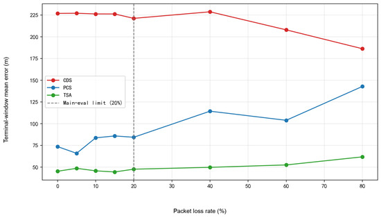
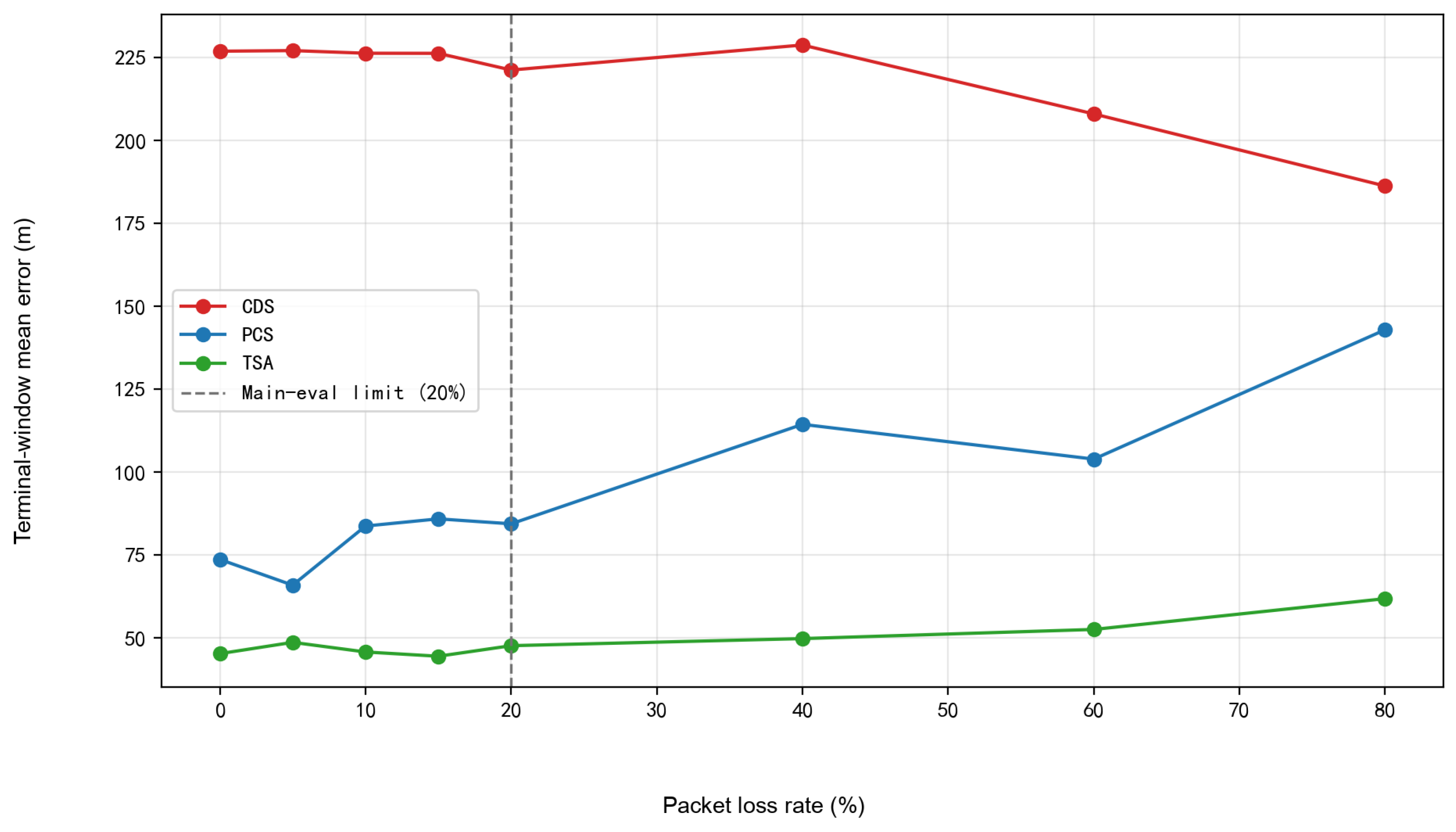
As shown in Figure 7 and Table 6, within the main evaluation interval of 0–$20\%$, the terminal-window mean sample-wise three-axis RMS position error of CDS remains at about 221–$227\mathrm{m}$, indicating that its dominant error source is still the spatiotemporal mismatch caused by direct fusion of delayed measurements. Therefore, the $L=0.107$ value of CDS is small, but this mainly reflects the limited relative variation around a high-error baseline and should not be interpreted as strong packet-loss robustness. The error of PCS fluctuates between $65.98$ and $85.97\mathrm{m}$, and its $L=1.125$ is the largest among the three, indicating that its compensation gain is most sensitive to the arrival condition of remote packets. TSA maintains a low error level of $44.55$–$48.74\mathrm{m}$ in the main evaluation interval, and its $L=0.028$ is the smallest, showing that Timestamp-Aligned Replay is more stable under small packet-loss disturbances. Since random loss of remote packets changes the temporal combination by which delayed measurements enter the filter, the errors of the algorithms need not vary strictly monotonically with packet-loss rate. Therefore, the comparison here focuses on the packet-loss response intensity L within the main evaluation interval. Figure 7 use the y-axis term “Terminal-window mean error” for ${ϵ}_{\pi ,\mathrm{term}}$, i.e., the mean of the sample-wise three-axis RMS position error over 80–$100\mathrm{s}$ and all Monte Carlo trials.

Figure 7. Terminal-window mean error under the packet-loss scan (${\mu }_{\tau }=1.0\mathrm{s}$, ${\sigma }_{\tau }=0.3\mathrm{s}$).

Table 6. Terminal-window mean sample-wise three-axis RMS position error under different packet-loss rates.

Packet-Loss Rate ${\mathit{p}}_{\mathbf{loss}}$ (%)	CDS Terminal-Window Error Mean ± std (m)	PCS Terminal-Window Error Mean ± std (m)	TSA Terminal-Window Error Mean ± std (m)
0	$226.99\pm 15.83$	$73.74\pm 75.04$	$45.33\pm 7.94$
5	$227.17\pm 16.55$	$65.98\pm 60.31$	$48.74\pm 31.45$
10	$226.37\pm 17.49$	$83.81\pm 92.65$	$45.84\pm 7.19$
15	$226.34\pm 17.94$	$85.97\pm 97.20$	$44.55\pm 8.10$
20	$221.31\pm 12.52$	$84.48\pm 91.08$	$47.74\pm 7.71$

4.3.5. Composite Evaluation and Partial-Order Comparison

As shown in Table 7, the metrics B, S, J, L, and the composite score of each algorithm summarize the communication-disturbance response evaluation results. This response vector is constructed exclusively from the terminal-window mean sample-wise three-axis RMS position errors of the baseline communication link and the average-delay, delay-jitter, and packet-loss scans reported in Table 3, Table 4, Table 5 and Table 6. Table 7 includes B in the primary partial order. TSA is smaller than CDS and PCS in all four dimensions and therefore Pareto-dominates both algorithms independently of weights. The normalized score is retained as a secondary result. PCS substantially improves B relative to CDS, while its larger J and L show sensitivity to the local reference trajectory and packet availability. The extreme CDS delay cell dominates its S value.

Table 7. $(B,S,J,L)$ metrics and Pareto comparison.

Algorithm	B	S	J	L	${\mathbf{\Gamma }}^{\mathbf{BSJL}}$	$(\mathit{B},\mathit{S},\mathit{J},\mathit{L})$ Partial Order
CDS	226.70	$5.11\times {10}^6$	10.57	0.107	0.677	Dominated by TSA
PCS	48.86	63.22	21.57	1.125	0.412	Dominated by TSA
TSA	42.45	30.84	5.55	0.028	0.000	Dominates CDS and PCS

4.3.6. OOSM-CKF Comparison

The following supplementary experiments use the same terminal-window mean sample-wise three-axis RMS position error as the principal communication scans.

The OOSM-CKF reference follows the delayed-time update route in [35]. When a packet generated at $t_j$ arrives at $t_k$, it performs one remote-bearing update at $t_j$, predicts the corrected state to $t_k$ without reprocessing the intervening measurements, and fuses the propagated correction with the current estimate. TSA instead re-executes the complete CKF sequence from the earliest newly activated timestamp to $t_k$, so the local measurements and previously activated remote measurements within that interval are used again. If several packets are released in one fusion interval, TSA activates all newly valid records before starting one replay from the earliest generation index.

Table 8 compares the six processing paths at five delay-jitter levels under ${\mu }_{\tau }=1.0\mathrm{s}$ and $p_{\mathrm{loss}}=5\%$, with 20 Monte Carlo trials per cell. A trial is classified as divergent when its terminal-window error exceeds $500\mathrm{m}$.

Table 8. Out-of-sequence measurement(OOSM) delay-jitter comparison using terminal-window mean sample-wise three-axis RMS position error.

${\mathit{\sigma }}_{\mathit{\tau }}$ (s)	CDS	PCS	TSA	Age-Limited Direct	Local	OOSM-CKF
0.10	$229.10\pm 23.77$ (5%)	$55.88\pm 20.53$ (0%)	$48.98\pm 6.73$ (0%)	$229.10\pm 23.77$ (5%)	$1681.00\pm 872.66$ (95%)	$1072.22\pm 576.73$ (85%)
0.30	$222.79\pm 20.47$ (0%)	$52.75\pm 17.39$ (0%)	$45.40\pm 5.25$ (0%)	$222.79\pm 20.47$ (0%)	$1681.00\pm 872.66$ (95%)	$1082.65\pm 582.92$ (85%)
0.50	$223.44\pm 43.47$ (5%)	$49.80\pm 23.57$ (0%)	$45.01\pm 6.09$ (0%)	$213.95\pm 17.18$ (0%)	$1681.00\pm 872.66$ (95%)	$1109.85\pm 591.12$ (85%)
1.00	$163.06\pm 12.94$ (0%)	$59.34\pm 56.27$ (0%)	$41.27\pm 5.81$ (0%)	$163.05\pm 12.95$ (0%)	$1681.00\pm 872.66$ (95%)	$1243.76\pm 657.05$ (90%)
2.00	$84.71\pm 23.12$ (0%)	$36.56\pm 9.37$ (0%)	$39.53\pm 7.74$ (0%)	$84.71\pm 23.12$ (0%)	$1681.00\pm 872.66$ (95%)	$1416.03\pm 736.48$ (90%)

TSA gives the lowest mean error at four of the five tested jitter levels and maintains zero divergence throughout the scan. Considering the mean errors, dispersion, and divergence statistics across all five levels, TSA provides better localization accuracy and stability under the tested conditions.

4.3.7. PCS Covariance-Inflation Structure Ablation

Section 3 defines the PCS gate and covariance-inflation structure, and Section 4.1 lists the numerical configuration used in the comparisons. Because the migrated angular residual depends on target range, platform displacement, and target maneuver, PCS inflates the migrated-measurement covariance to reduce the influence of measurements with large delay or innovation in the current update.

The experiment compares $q\equiv 1$, delay-only inflation, innovation-only inflation, and the complete rule at eight average-delay levels, with 10 Monte Carlo trials at each parameter point. Table 9 reports the corresponding Monte Carlo means and empirical standard deviations.

Table 9. PCS covariance-inflation ablation using terminal-window mean sample-wise three-axis RMS position error.

${\mathit{\mu }}_{\mathit{\tau }}$ (s)	$\mathit{q}\equiv 1$	Delay Only	Innovation Only	Complete q
0.20	$33.24\pm 7.93$	$38.23\pm 12.66$	$46.50\pm 28.88$	$46.76\pm 31.59$
0.53	$42.31\pm 25.98$	$50.54\pm 32.73$	$29.71\pm 8.65$	$58.96\pm 51.41$
0.86	$31.44\pm 8.38$	$111.18\pm 130.39$	$30.41\pm 7.26$	$59.46\pm 20.65$
1.19	$38.30\pm 8.66$	$62.90\pm 35.80$	$35.74\pm 8.37$	$89.01\pm 89.62$
1.51	$45.81\pm 7.52$	$121.37\pm 153.57$	$40.30\pm 11.61$	$141.31\pm 144.54$
1.84	$71.01\pm 38.14$	$82.19\pm 62.53$	$58.50\pm 20.54$	$112.58\pm 112.84$
2.17	$174.48\pm 86.70$	$105.43\pm 112.12$	$183.75\pm 219.38$	$86.15\pm 40.30$
2.50	$213.59\pm 95.07$	$206.16\pm 210.30$	$189.49\pm 80.03$	$226.22\pm 216.14$

Table 9 shows that different inflation structures have different advantages across the tested average-delay conditions and that no structure uniformly dominates all tested points. These results characterize structural sensitivity under the current average-delay scan rather than identify a universally optimal PCS form. The complete q represents uncertainty associated with both delay growth and innovation magnitude and shows favorable overall performance in the preceding baseline, average-delay, delay-jitter, and packet-loss experiments; it is therefore retained as the main PCS implementation in this study.

4.3.8. PCS Covariance-Inflation Coefficient Sensitivity

To further examine the sensitivity of the complete PCS rule to its delay-related coefficients, Table 10 selects six representative configurations from the coefficient scan: two lower-inflation settings, the $(4,8)$ configuration used in the principal experiments, and three settings with a large quadratic-delay coefficient. Each configuration is evaluated at the eight average-delay levels

$${\mu }_{\tau }\in \{0.20,0.53,0.86,1.19,1.51,1.84,2.17,2.50\}\mathrm{s},$$

with 10 Monte Carlo trials per delay level. The analysis holds $c_{\rho }=1.5$, ${\rho }_0=0.02\mathrm{rad}$, and ${\rho }_{\max }=0.12\mathrm{rad}$ fixed.

Table 10. Representative configurations for the sensitivity of the PCS delay-related coefficients.

$({\mathit{c}}_{\mathit{t}},{\mathit{c}}_{\mathbf{tt}})$	Role	Mean (m)	Median (m)	p95 (m)	Max (m)
$(1,2)$	Lower-inflation setting	44.03	45.50	71.60	80.78
$(2,2)$	Lower-inflation setting	44.72	44.58	68.95	88.17
$(4,8)$	Configuration used in principal scans	74.49	50.08	262.99	579.43
$(1,16)$	Large quadratic-term setting	101.53	53.98	444.47	708.72
$(4,16)$	Large quadratic-term setting	114.91	56.17	544.55	633.01
$(8,16)$	Large quadratic-term setting	114.35	59.63	454.86	664.73

Table 10 shows that the complete q rule is sensitive to its delay-related coefficients. The displayed lower-inflation settings have smaller central and upper-tail errors on the current average-delay grid, whereas a large quadratic-delay coefficient can increase the long-delay error tail. These representative results characterize coefficient sensitivity rather than reselect the parameters used in the principal experiments. To maintain a consistent PCS definition and parameterization across the baseline, average-delay, delay-jitter, and packet-loss scans, the principal experiments retain the $(4,8)$ configuration. Multi-condition parameter optimization and online adaptation remain topics for future work.

4.3.9. TSA Buffer-Length Sensitivity

To examine the relation between replay coverage and computational cost, $L_b\in \{10,20,40,60,80\}$ is tested under the baseline communication link, with 20 Monte Carlo trials for each buffer length. At the sampling period $T=0.05\mathrm{s}$, the nominal buffer duration is $L_{b}T$, while the actual index span between the earliest and current nodes is $(L_b-1)T$. Table 11 reports the terminal-window mean sample-wise three-axis RMS position error and the mean runtime per complete trial.

Table 11. Effects of TSA buffer length on localization error and runtime under the baseline communication link.

${\mathit{L}}_{\mathit{b}}$ (Nodes)	Nominal Duration (s)	Terminal-Window Error ± SD (m) ($\mathit{n}=20$)	Mean Runtime/Tial (s)
10	0.50	$81.36\pm 62.37$	3.87
20	1.00	$60.47\pm 42.65$	18.59
40	2.00	$42.90\pm 4.16$	47.78
60	3.00	$45.64\pm 8.44$	56.34
80	4.00	$44.80\pm 7.79$	57.48

The 10-node window has the largest mean error and dispersion, and the 20-node result remains highly variable. Over $L_b=40$–80, the mean errors range from $42.90$ to $45.64\mathrm{m}$; $L_b=40$ gives the lowest mean, the smallest standard deviation, and lower runtime than the 60- and 80-node settings. Thus, $L_b=40$ provides the best balance between replay coverage, localization stability, and computational time among the tested buffer lengths.

For the baseline link,

$${\mu }_{\tau }+3{\sigma }_{\tau }=1.0+3\times 0.3=1.9\mathrm{s}<1.95\mathrm{s},$$

(75)

so the selected window covers the principal range of the baseline delay distribution. For a time-varying communication link, the buffer length can be adjusted according to online estimates of the delay mean and standard deviation:

$$L_b\left(k\right)=\mathrm{clip}\left(⌈{\displaystyle \frac{{\widehat{\mu }}_{\tau }\left(k\right)+c{\widehat{\sigma }}_{\tau }\left(k\right)}{T}}⌉,L_{\min },L_{\max }\right),$$

(76)

where c is a coverage coefficient, $L_{\min }$ prevents an excessively short replay window, and $L_{\max }$ bounds memory and worst-case replay cost. The rule expands the replay window as communication delay increases and reduces computation and storage when link conditions improve. The reported numerical comparisons retain the fixed value $L_b=40$; the adaptive rule is presented as an extension for time-varying links.

4.3.10. Complexity, Average Throughput, and Memory

For state dimension n, TSA has replay cost $O\left({\mathcal{l}}_k{C}_{\mathrm{CKF}}\left(n\right)\right)$, where ${\mathcal{l}}_k\le L_b$, and numeric cache storage $O\left(L_b{n}^2\right)$. Table 12 is dedicated to computational time and memory. It reports runtime statistics over 20 complete 100-s trials together with separately measured peak memory; the equivalent average time per step is obtained by dividing the mean trial time by 2000 fusion steps.

Table 12. Runtime and peak memory of the compared strategies.

Strategy	Trial Time (s)	Equivalent Average Time/Step (ms)	Peak Memory (MB)
CDS	$2.71\pm 0.08$	1.35	1.03
PCS	$4.03\pm 0.10$	2.02	1.17
TSA	$39.57\pm 0.71$	19.78	4.29
OOSM-CKF	$38.26\pm 0.35$	19.13	2.56
Local	$2.98\pm 0.05$	1.49	1.00
Age-Limited Direct	$2.76\pm 0.10$	1.38	1.01
Ideal	$2.67\pm 0.10$	1.34	1.00

TSA requires an equivalent average time of $19.78\mathrm{ms}$ per step, approximately 14.7 and 9.8 times those of CDS and PCS, respectively, and its peak memory is $4.29\mathrm{MB}$. The results show that replay increases both computation and storage while maintaining timestamp-aligned processing. The reported value is derived from complete-trial wall-clock time and represents average throughput rather than measured per-update latency.

4.3.11. Bearing-Noise Sensitivity

The azimuth- and elevation-noise standard deviations are set to $0.9$, $1.8$, $3.6$, and $7.2\mathrm{mrad}$, with 20 Monte Carlo trials at each level. As shown in Table 13, at $0.9$ and $1.8\mathrm{mrad}$, TSA gives the lowest mean error with zero divergence. At $3.6\mathrm{mrad}$ and above, all three methods show substantial increases in error and divergence rate, demonstrating the strong dependence of bearing-only cooperative localization on angular-measurement accuracy.

Table 13. Bearing-noise sensitivity using terminal-window mean sample-wise three-axis RMS position error.

${\mathit{\sigma }}_{\mathit{\theta }}$ (mrad)	CDS	PCS	TSA
0.9	$231.25\pm 14.40$ (0%)	$142.78\pm 69.19$ (0%)	$30.13\pm 2.67$ (0%)
1.8	$222.79\pm 20.47$ (0%)	$52.74\pm 17.37$ (0%)	$45.41\pm 5.26$ (0%)
3.6	$362.50\pm 226.82$ (45%)	$(2.67\times {10}^5)\pm (7.46\times {10}^5)$ (70%)	$483.95\pm 339.57$ (70%)
7.2	$(1.41\times {10}^6)\pm (5.18\times {10}^6)$ (95%)	$(5.51\times {10}^5)\pm (6.54\times {10}^5)$ (85%)	$(8.46\times {10}^6)\pm (2.47\times {10}^7)$ (95%)

5. Discussion

TSA belongs to the finite-lag buffer-and-reprocess OOSM family. Its application-specific implementation records the bearing, generation timestamp, dual-platform geometry, measurement availability, and CKF state at each retained index. In contrast to the OOSM-CKF reference used here, which applies one delayed-time update followed by open-loop prediction and current-time fusion, TSA reprocesses the complete retained interval and reuses the intervening local and activated remote measurements. Table 8 shows that this complete-interval processing provides the lowest mean error among the six compared strategies at four of the five tested jitter levels and maintains zero divergence throughout the scan. Considering the mean errors, dispersion, and divergence statistics, TSA provides better localization accuracy and stability under the tested conditions.

PCS avoids replay and therefore has a lower computational cost, but the migrated angular innovation depends on target range, platform displacement, and target maneuver. The explicit covariance-inflation function $q(\Delta t,\rho )$ reduces the weight of measurements with large delay or innovation. The structure ablation and coefficient-sensitivity results reveal trade-offs among different configurations, but the present one-dimensional average-delay analyses are insufficient to identify a universally optimal PCS. The complete q retains favorable overall performance in the four principal communication experiments and is therefore used as the PCS implementation in this study. PCS remains a low-cost approximate compensation option, while broader multi-condition parameter selection and online adaptation require further investigation.

The dual-UAV system is the smallest unit of multi-platform cooperative localization. For N UAVs, the measurement vector can be extended to $2N$ angular components while the target-state dimension remains unchanged. A centralized method maintains timestamped availability flags and platform geometry for each UAV and starts replay from the oldest newly valid packet. A distributed extension must additionally address inter-node information correlation and consensus fusion [11,12,17,18]; fixed-time consensus methods provide a reference for cooperative information convergence in multi-agent systems [39]. As the number of platforms and maximum lag increase, concurrent packet scheduling, cache storage, and replay computation grow together.

The simulations use a representative dual-UAV geometry and a target trajectory dominated by horizontal turns, with UAV position and attitude treated as known inputs. The results therefore describe algorithm behavior under the tested communication-disturbance conditions. The reported runtime reflects average software throughput rather than per-update or worst-case execution time.

Future work will extend the evaluation to broader platform separations and headings, initial observation geometries, target speeds and three-dimensional maneuvers, and will incorporate platform-state uncertainty, joint PCS parameter validation across multidimensional communication conditions, online adjustment of PCS parameters and replay windows, incremental parallel computing, embedded-platform timing, multi-UAV cooperative fusion, and synchronized flight experiments.

6. Conclusions

This article investigated late-arriving remote bearing measurements in dual-UAV cooperative passive localization under communication uncertainty. Within a unified CKF framework, PCS performs predictive compensation through historical-innovation migration and covariance inflation, whereas TSA restores the dual-platform observation geometry at the generation time of a delayed measurement and propagates the historical correction to the current output through finite-lag replay. The timestamped cache, packet-ordering procedure, and state-overwrite rules jointly ensure consistency in delayed-measurement processing.

Under the tested configuration, the numerical results show that direct fusion of late measurements is vulnerable to mismatch among timestamps, platform geometry, and the current target state. PCS can exploit part of the delayed-measurement information at relatively low computational cost, but its performance depends on the covariance-inflation structure and parameter settings. By restoring the dual-platform geometry at the measurement generation time and performing finite-lag replay, TSA provides lower and more stable localization error under communication disturbances. The buffer-length and bearing-noise analyses further show that computational resources, observation accuracy, and replay coverage jointly affect accuracy, stability, and online implementation cost.

The results demonstrate that aligning delayed bearing measurements with the platform geometry and target state at their generation time can effectively improve cooperative-localization accuracy under communication delay, delay jitter, and packet loss.

References

- Li, X.; Willett, P.; Baum, M.; Li, Y. PMHT approach for underwater bearing-only multisensor–multitarget tracking in clutter. IEEE J. Ocean. Eng. 2016, 41, 831–839. [Google Scholar] [CrossRef] [Scilit]
- Shalev, H.; Klein, I. BOTNet: Deep learning-based bearings-only tracking using multiple passive sensors. Sensors 2021, 21, 4457. [Google Scholar] [CrossRef] [Scilit] [PubMed]
- Zhou, Y.; Wang, D.; Li, J. Consensus 3-D bearings-only tracking in switching sensor networks. Signal Process. 2014, 105, 148–155. [Google Scholar] [CrossRef] [Scilit]
- Lin, J.; Xiao, W.; Lewis, F.L.; Xie, L. Energy-efficient distributed adaptive multisensor scheduling for target tracking in wireless sensor networks. IEEE Trans. Instrum. Meas. 2009, 58, 1886–1896. [Google Scholar] [CrossRef] [Scilit]
- Yin, Q.; Xu, C.; Zhou, P.; Huang, D.; Xu, W. Dual-UAV cooperative bearing-only target localization based on multi-level box particle filter. Digit. Signal Process. 2026, 168, 105572. [Google Scholar] [CrossRef] [Scilit]
- Qian, M.; Chen, W.; Sun, R. A Maneuvering Target Tracking Algorithm Based on Cooperative Localization of Multi-UAVs With Bearing-Only Measurements. IEEE Trans. Instrum. Meas. 2024, 73, 9516911. [Google Scholar] [CrossRef] [Scilit]
- Aidala, V.J. Kalman filter behavior in bearings-only tracking applications. IEEE Trans. Aerosp. Electron. Syst. 1979, 15, 29–39. [Google Scholar] [CrossRef] [Scilit]
- Nardone, S.C.; Aidala, V.J. Observability criteria for bearings-only target motion analysis. IEEE Trans. Aerosp. Electron. Syst. 1981, 17, 162–166. [Google Scholar] [CrossRef] [Scilit]
- Aidala, V.J.; Hammel, S.E. Utilization of modified polar coordinates for bearings-only tracking. IEEE Trans. Autom. Control 1983, 28, 283–294. [Google Scholar] [CrossRef] [Scilit]
- Anjaly, P.; Ratnoo, A. Observability enhancement of maneuvering target with bearings-only information. J. Guid. Control Dyn. 2018, 41, 184–198. [Google Scholar] [CrossRef] [Scilit]
- Fan, Y.; Meng, F.; Li, G.; Qi, X. A survey and evaluation of iterative optimization algorithms for cooperative localization. Phys. Commun. 2023, 60, 102165. [Google Scholar] [CrossRef] [Scilit]
- Sun, Q.; Tian, Y.; Diao, M. Cooperative localization algorithm based on hybrid topology architecture for multiple mobile robot system. IEEE Internet Things J. 2018, 5, 4753–4763. [Google Scholar] [CrossRef] [Scilit]
- Li, J.; Yang, G.; Cai, Q.; Niu, H.; Li, J. Cooperative navigation for UAVs in GNSS-denied area based on optimized belief propagation. Measurement 2022, 192, 110797. [Google Scholar] [CrossRef] [Scilit]
- Sinopoli, B.; Schenato, L.; Franceschetti, M.; Poolla, K.; Jordan, M.I.; Sastry, S.S. Kalman filtering with intermittent observations. IEEE Trans. Autom. Control 2004, 49, 1453–1464. [Google Scholar] [CrossRef] [Scilit]
- Schenato, L. Optimal estimation in networked control systems subject to random delay and packet drop. IEEE Trans. Autom. Control 2008, 53, 1311–1317. [Google Scholar] [CrossRef] [Scilit]
- Hespanha, J.P.; Naghshtabrizi, P.; Xu, Y. A survey of recent results in networked control systems. Proc. IEEE 2007, 95, 138–162. [Google Scholar] [CrossRef] [Scilit]
- Zhang, Z.; Dong, X.; Yv, J.; Li, Q.; Ren, Z. Distributed cooperative tracking and cooperative guidance against maneuvering aerial target. Aerosp. Sci. Technol. 2024, 144, 108827. [Google Scholar] [CrossRef] [Scilit]
- Liu, Y.; Wang, Y.; Shen, Y.; Shi, X. Hybrid TOA-AOA WLS estimator for aircraft network decentralized cooperative localization. IEEE Trans. Veh. Technol. 2023, 72, 9670–9675. [Google Scholar] [CrossRef] [Scilit]
- Kalman, R.E. A New Approach to Linear Filtering and Prediction Problems. J. Basic Eng. 1960, 82, 35–45. [Google Scholar] [CrossRef] [Scilit]
- Julier, S.J.; Uhlmann, J.K. Unscented filtering and nonlinear estimation. Proc. IEEE 2004, 92, 401–422. [Google Scholar] [CrossRef] [Scilit]
- Arasaratnam, I.; Haykin, S. Cubature Kalman filters. IEEE Trans. Autom. Control 2009, 54, 1254–1269. [Google Scholar] [CrossRef] [Scilit]
- Li, X.R.; Jilkov, V.P. Survey of maneuvering target tracking. Part V: Multiple-model methods. IEEE Trans. Aerosp. Electron. Syst. 2005, 41, 1255–1321. [Google Scholar] [CrossRef] [Scilit]
- Guo, X.; Liu, F.; Huang, D. Migration through resolution cell correction and sparse aperture ISAR imaging for maneuvering target based on whale optimization algorithm–fast iterative shrinkage thresholding algorithm. Sensors 2024, 24, 2148. [Google Scholar] [CrossRef] [Scilit] [PubMed]
- Li, J.; Yin, C.; Zhang, Y.; Diao, H. Phase error compensation method for maneuvering target based on image entropy minimization. Proc. SPIE 2024, 13180, 131806Z. [Google Scholar] [CrossRef] [Scilit]
- Dong, M.; Li, H.; Qin, Y.; Hu, Y.; Huang, H. A secure and accurate localization algorithm for mobile nodes in underwater acoustic network. Eng. Appl. Artif. Intell. 2024, 133, 108157. [Google Scholar] [CrossRef] [Scilit]
- Li, W.; Li, M.; Liu, A.; Han, T.X. Design and optimization of cooperative sensing with limited backhaul capacity. arXiv 2024, arXiv:2404.03440. [Google Scholar]
- Wei, Y.; Xie, J.; Gao, W.; Li, H.; Wang, L. A fully decentralized distributed learning algorithm for latency communication networks. Knowl.-Based Syst. 2025, 309, 112829. [Google Scholar] [CrossRef] [Scilit]
- Chen, L.; Tang, F.; Li, X.; Liu, J.; Yang, Y.; Yu, J.; Zhu, Y. Delay-optimal cooperation transmission in remote sensing satellite networks. IEEE Trans. Mob. Comput. 2023, 22, 5109–5122. [Google Scholar] [CrossRef] [Scilit]
- Ma, X.; Zhao, J.; Liao, J.; Zhang, Z. Intelligent reflecting surface-assisted federated learning in multi-platoon collaborative networks. Digit. Commun. Netw. 2023, 9, 628–637. [Google Scholar] [CrossRef] [Scilit]
- Yang, H.; Li, W.; Zhang, C.; Wang, J. Cloud-based cooperative merging control with communication delay compensation for connected and automated vehicles. Sustainability 2025, 17, 7952. [Google Scholar] [CrossRef] [Scilit]
- Ding, D.; Han, Q.-L.; Ge, X.; Zhang, X.-M.; Wang, J. Privacy-preserving filtering, control and optimization for industrial cyber-physical systems. Sci. China Inf. Sci. 2025, 68, 151201. [Google Scholar] [CrossRef] [Scilit]
- Challa, S.; Morelande, M.R.; Mušicki, D.; Evans, R.J. Fundamentals of Object Tracking; Cambridge University Press: Cambridge, UK, 2011. [Google Scholar]
- Mauthner, M.; Elmenreich, W.; Kirchner, A.; Boesel, D. Out-of-sequence measurements treatment in sensor fusion applications: Buffering versus advanced algorithms. In Workshop Fahrerassistenzsysteme; FAS: Washington, DC, USA, 2006. [Google Scholar]
- Bar-Shalom, Y. Update With Out-of-Sequence Measurements in Tracking: Exact Solution. IEEE Trans. Aerosp. Electron. Syst. 2002, 38, 769–777. [Google Scholar] [CrossRef] [Scilit]
- Bar-Shalom, Y.; Chen, H.; Mallick, M. One-step solution for the multistep out-of-sequence-measurement problem in tracking. IEEE Trans. Aerosp. Electron. Syst. 2004, 40, 27–37. [Google Scholar] [CrossRef] [Scilit]
- Shi, Y.; Farina, A.; Song, T.L.; Peng, D.; Guo, Y. Distributed fusion in harsh environments using multiple bearings-only sensors with out-of-sequence-refined measurements. Aerosp. Sci. Technol. 2021, 117, 106950. [Google Scholar] [CrossRef] [Scilit]
- Li, S.; Zou, N.; Qi, B.; Liang, G.; Li, X. Underwater multi-sensor multi-target bearing-only tracking based on delayed measurements. Signal Process. 2026, 238, 110134. [Google Scholar] [CrossRef] [Scilit]
- Zhang, F. A new method for double IRST cooperative passive detection and positioning for maneuvering target. Acta Aeronaut. Astronaut. Sin. 2020, 41, 322988. [Google Scholar]
- Parsegov, S.E.; Polyakov, A.E.; Shcherbakov, P.S. Fixed-time consensus algorithm for multi-agent systems with integrator dynamics. IFAC Proc. Vol. 2013, 46, 110–115. [Google Scholar] [CrossRef] [Scilit]
Disclaimer/Publisher’s Note: The statements, opinions and data contained in all publications are solely those of the individual author(s) and contributor(s) and not of MDPI and/or the editor(s). MDPI and/or the editor(s) disclaim responsibility for any injury to people or property resulting from any ideas, methods, instructions or products referred to in the content. |
© 2026 by the authors. Licensee MDPI, Basel, Switzerland. This article is an open access article distributed under the terms and conditions of the Creative Commons Attribution (CC BY) license.